Embed Size (px)
Citation preview
PhD thesis
Ayman B. T. Attya

„Gedruckt mit Unterstützung des Deutschen Akademischen Austauschdienstes―
Wind energy penetration impact on grid frequency during normal operation and frequency deviations
Dem Fachbereich Elektrotechnik und Informationstechnik
der Technischen Universität Darmstadt
zur Erlangung des akademischen Grades eines
Doktor-Ingenieurs (Dr.-Ing.)
genehmigte Dissertation
von
Ayman Bakry Taha Attya, M.Sc.
Geboren am 17.05.1983 in Giza, Ägypten
Referent: Prof. Dr. Thomas Hartkopf
Korreferent: Prof. Dr. Gerd Griepentrog
Extern Korreferent: Prof. Dr. Yasser Hegazy
Tag der Einreichung: 11.06.2014
Tag der mündlichen Prüfung: 30.09.2014
D 17
Darmstadt 2014

Erklärung laut §9 Promo
Ich versichere hiermit, dass ich die vorliegende Dissertation allein und nur unter Verwendung der
angegebenen Literatur verfasst habe. Die Arbeit hat bisher noch nicht zu Prüfungszwecken gedient.

Preface i
Preface
Due to increasing wind power penetration the power system impact of wind power is a relevant aspect
of research. The present PhD thesis deals with possible support algorithms for wind turbines to
participate positively in frequency drops mitigation. Comprehensive dynamic simulation models for
wind turbines and conventional generators are integrated in order to simulate their interaction during
frequency deviations. In the present thesis, storage mediums are also investigated as a solution for
wind energy intermittent nature and its impact on frequency response. The Egyptian case study real
and chronological data acquired from related authorities is considered as a benchmark system for the
examined algorithms.
The PhD research was carried out in the Institute of Electrical Power Systems - Department of
Renewable Energies at Technical University of Darmstadt (Germany). This research work is funded
through cooperation between the Egyptian ministry of high education and research from one side and
the DAAD (German Academic Exchange Service) from the other side. The duration of the scholarship
was from April 2011 till September 2014.

Summary ii
Summary
The fluctuating nature of output from wind farms in relation to wind speed conditions at each wind
turbine causes a severe burden on conventional generators, and such wind power variations have a
considerable impact on grid frequency and voltage stability. In addition, such fluctuations in output
create economic problems, as most of system operators apply financial penalties on wind farms
owners when generation levels deviate from forecasted schedules by certain ratios. This thesis focuses
on the negative impacts of moderate and high levels of wind power contribution to grid generation
capacities on the frequency response. Particularly, integrated wind farms replace certain ratios from
conventional generation capacity. Retired conventional capacity is decided according to estimated
annual energy production of installed wind farms.
The work presented here focuses on the contribution of wind turbines in the curtailment of frequency
drops. Specifically, two algorithms are proposed to provide a predetermined increase in wind farms
active power to support the system and mitigate the generation–demand imbalance. One algorithm
relates to the stored kinetic energy in the wind turbine rotating parts, and the other relates to the steep
rise in output power that is delivered when the wind turbine pitch angle given value in de-loading
operation, is reduced to zero. The two offered algorithms are compared mainly from the point of view
of energy utilization with respect to standard operation. A dispatching algorithm is also presented to
manage the number of wind turbines in each wind farm that should be switched to support mode, and
a modified method for estimating the retired conventional generation capacity is also presented. Thus,
the expected amounts of annual energy generated by different types of wind turbines in different sites
are evaluated based on the available chronological wind speeds records and network load. Finally, this
thesis discusses the feasibility and influence of integrating storage mediums, namely battery banks, as
a backup power source during frequency events.
Throughout all the mentioned analysis, frequency responses of several hypothetical and a genuine
system, namely, the Egyptian system, are examined in different case studies to investigate the impact
of the proposed algorithms on frequency performance. MATLAB and Simulink are the main software
applied. Results acquisition reveals the capability of wind farms on mitigating frequency drops. The
proposed algorithms are seen to deliver advantages and disadvantages, and selection based on
compromise is required to choose the best solutions that match the investigated case studies.

Zusammenfassung iii
Zusammenfassung
Die natürlichen Schwankungen der Leistung von Windparks aufgrund fluktuierender
Windgeschwindigkeiten haben einen nicht unerheblichen Einfluss auf die Qualität der
Stromversorgung. Die vorliegende Dissertation konzentriert sich daher auf den Einfluss von
Windparks auf die Frequenzstabilität in elektrischen Versorgungsnetzen. Dieser Einfluss ist wichtiger
und klarer wenn mehr Windparks konventionelle Generatoren auswechseln.
Es werden zwei spezielle Algorithmen vorgestellt, welche eine Erhöhung der aktiven
Windparkenergie ermöglichen, die Stabilität des Erzeugungssystems verbessern und die Bilanz von
Erzeugung und Nachfrage ausgleichen sollen. Der erste Algorithmus bezieht sich auf die in den
rotierenden Teilen der Windkraftanlage gespeicherte kinetischen Energie. Der zweite Algorithmus
betrifft den Blatteinstellwinkel, der die Drehgeschwindigkeit des Rotors verändern kann. Während des
normalen Betriebs bei entsprechendem Wind ist der Blatteinstellwinkel größer als Null und sinkt,
wenn ein Frequenzabfall eintritt. Die beiden hier vorgestellten Algorithmen werden dabei
hauptsächlich aus dem Blickwinkel der Energienutzung mit Bezug auf den Normalbetrieb verglichen.
Die vorliegende Forschungsarbeit bietet auf Basis chronologischen Daten für Netzbelastung und
Windgeschwindigkeit auch eine neue Methode zur Berechnung der jährlichen Energieproduktion der
Windkraftanlagen. Zusätzlich ist eine neue ‚Dispatch‗-Methode in die Algorithmen integriert, welche
die Unterstützungsrolle für jede Windkraftanlage in jedem Windpark während eines
Frequenzproblems definiert.
Eine neuartige Lösung zur Einbeziehung von Speichermedien, insbesondere Batteriebänken, wird zum
Abschluss der Arbeit vorgeschlagen und die Energiekapazität sowie die Leistung der Batterien
bewertet. Der Einsatz der Batterien zielt zunächst auf eine Aufladung während des Normalbetriebs
und bei guten Windkonditionen ab. Danach sind die Batterien in der Lage, zusätzliche Wirkleistung zu
liefern, um einem plötzlichen Frequenzabfall unter bestimmten Bedingungen entgegenwirken zu
können.
Die gesamte Analyse wird anhand hypothetischer Systeme und anschließend für das ägyptische Netz
und die dortige Windenergienutzung untersucht. Alle Fallstudien vergleichen und analysieren die
Frequenzkurven vor und nach der Integration der präsentierten Methoden und zeigen deren Vor- und
Nachteile auf. Als primäre Simulationssoftware wurden MATLAB und Simulink verwendet. Es hat
sich ergeben, dass die hier vorgeschlagenen Algorithmen zwar das Potential zur Minderung von
plötzlichen Frequenzabfällen besitzen, aber dennoch eine kompromissbasierte Auswahl nötig ist, um
die optimale Lösung für die jeweils untersuchte Fallstudie zu finden.

Contents iv
Contents
1. Introduction ..................................................................................................................................... 1
1.1. Motivation ............................................................................................................................... 1
1.2. Wind turbine concepts ............................................................................................................. 3
1.3. Wind speed model ................................................................................................................... 4
1.4. Research objectives ................................................................................................................. 5
1.5. Thesis layout............................................................................................................................ 6
2. Wind energy integration in power systems ..................................................................................... 8
2.1. Wind turbine concepts and modelling ..................................................................................... 8
2.1.1. Wind turbines types ............................................................................................................... 8
2.1.2. Modelling aspects of wind turbines ..................................................................................... 11
2.2. Wind turbine operational modes ........................................................................................... 15
2.3. Wind turbines ride through and support algorithms .............................................................. 17
2.3.1. Low voltage ride through – methods and aims.................................................................... 17
2.3.2. Frequency drops ride through and support - methods and aims .......................................... 19
2.4. Wind speed prospects and simulation ................................................................................... 22
2.5. Wind farm aggregation .......................................................................................................... 23
2.6. Wind farms‘ dispatching ....................................................................................................... 25
2.7. The integration of storage mediums ...................................................................................... 26
3. Method 1: Wind turbine over speeding and kinetic energy extraction .......................................... 28
3.1. Wind turbine rotor speed variations ...................................................................................... 28
3.2. Proposed algorithm................................................................................................................ 29
3.3. Implemented benchmark system and case studies ................................................................ 34
3.3.1. Benchmark system .............................................................................................................. 34
3.3.2. Case studies ......................................................................................................................... 35
3.4. Results and Discussion .......................................................................................................... 37
3.4.1. Impact on system frequency response ................................................................................. 38
3.4.2. Attitude of the main parameters of the proposed algorithm ................................................ 42
3.5. Summary ............................................................................................................................... 46

Contents v
4. Method 2: Wind turbine de-loading/overloading .......................................................................... 47
4.1. Proposed algorithm................................................................................................................ 47
4.1.1. Wind speed categories ......................................................................................................... 47
4.1.2. Operational regions ............................................................................................................. 48
4.2. Case studies ........................................................................................................................... 55
4.2.1. Case study 1: Support energy estimation ............................................................................ 55
4.2.2. Case Study 2: Implementation using a hypothetical system ............................................... 56
4.3. Results and Discussion .......................................................................................................... 58
4.3.1. Case study 1......................................................................................................................... 58
4.3.2. Case study 2......................................................................................................................... 59
4.4. Summary ............................................................................................................................... 61
5. Comparison of proposed support methods .................................................................................... 62
5.1. Maximum power tracking operation: .................................................................................... 62
5.1.1. Manufacturer power curve (MPT 1) .................................................................................... 62
5.1.2. Optimum power evaluation using Cp equation (MPT 2) ..................................................... 62
5.2. Frequency Support techniques .............................................................................................. 63
5.2.1. Over-speeding operation (Method 1) .................................................................................. 63
5.2.2. Standard de-loading operation ............................................................................................. 63
5.2.3. Partial de-loading algorithm (Method 2) ............................................................................. 64
5.3. Wasted energy assessment .................................................................................................... 64
5.4. Case studies ........................................................................................................................... 65
5.5. Results and discussion ........................................................................................................... 66
5.5.1. Performance curves comparison .......................................................................................... 66
5.5.2. Wasted energy analysis ....................................................................................................... 68
5.6. Summary ............................................................................................................................... 69
6. Wind farm energy production assessment – an Egyptian case study ............................................ 70
6.1. Replacement of conventional generation by WFs ................................................................. 70
6.1.1. Annual energy production assessment ................................................................................ 71
6.1.2. Matching wind turbines with wind farms locations ............................................................ 72
6.2. Egypt - grid and wind energy prospects ................................................................................ 73

Contents vi
6.2.1. Egyptian grid ....................................................................................................................... 73
6.2.2. Promising locations for wind farms .................................................................................... 73
6.3. Implementation of proposed algorithm ................................................................................. 74
6.4. Frequency response during normal operation ....................................................................... 77
6.4.1. Test system description ....................................................................................................... 77
6.4.2. Frequency response analysis ............................................................................................... 78
6.5. Summary ............................................................................................................................... 80
7. Wind farms dispatching during frequency drops .......................................................................... 81
7.1. Proposed algorithm................................................................................................................ 81
7.1.1. Estimation of required overall active power support from installed WFs ........................... 82
7.1.2. Estimating the required power step from each WF ............................................................. 83
7.1.3. The evaluation of the number of participating clusters in the support process ................... 83
7.2. Test system and case Studies ................................................................................................. 85
7.2.1. Test system .......................................................................................................................... 85
7.2.2. Case studies ......................................................................................................................... 86
7.3. Results and discussion ........................................................................................................... 88
7.3.1. System frequency responses ................................................................................................ 88
7.3.2. Power generation variations ................................................................................................ 91
7.3.3. Attitude of the main parameters of the proposed algorithm ................................................ 93
7.4. Summary ............................................................................................................................... 96
8. Storage banks for frequency support purposes .............................................................................. 97
8.1. Assessment of storage banks rated power ............................................................................. 97
8.2. Storage bank operation ........................................................................................................ 100
8.2.1. Normal Operation .............................................................................................................. 100
8.2.2. Support Operation ............................................................................................................. 101
8.3. Test system and case studies ............................................................................................... 102
8.3.1. Test system ........................................................................................................................ 102
8.3.2. Case studies ....................................................................................................................... 102
8.4. Results and discussion ......................................................................................................... 104
8.5. Summary ............................................................................................................................. 109

Contents vii
9. Conclusions, recommendations, and future work ....................................................................... 110
10. Bibliography ............................................................................................................................ 113
11. Appendix ................................................................................................................................. 119
11.1. List of figures .................................................................................................................. 119
11.2. List of tables .................................................................................................................... 121
11.3. List of abbreviations ........................................................................................................ 122
11.4. Nomenclature .................................................................................................................. 123
11.5. Method 1 mathematical derivations ................................................................................ 126
11.6. Tables .............................................................................................................................. 128
11.7. Figures ............................................................................................................................. 133
Related publications ............................................................................................................................ 134
International peer reviewed journals ............................................................................................... 134
International peer reviewed conferences‘ proceedings ................................................................... 134
Acknowledgement ............................................................................................................................... 135
Academic career .................................................................................................................................. 136
Employment history ........................................................................................................................ 136
Education ......................................................................................................................................... 136
Master thesis topic ........................................................................................................................... 136

Introduction 1
Throughout the world, electrical energy is a priority issue for governments, companies, and research
institutes, and varying viewpoints are continually be presented in relation to the optimum priorities of
generation technologies in both developed and developing countries. For example, developed
countries are mainly concerned with the reduction of pollution emissions caused by conventional
power plants using fossil fuels such as coal and oil. In the past, nuclear energy was a favourite option
for some of these countries, but due to a number of global accidents (such as the tsunami disaster in
Japan that caused destruction of nuclear reactors with catastrophic consequence) nuclear reactors are
now being perceived as potential threats. Developing countries are seeking solutions for the mitigation
of high conventional energy prices and for the political and economic limitations imposed on them in
relation to building nuclear reactors. Consequently, renewable energy provides a solution for both
teams. Solar, wind, biomass, geothermal, and tidal energies are well known examples of renewable
energy resources that are widely used globally at different rates and levels of technology [1].
However, solar and wind power generation are the most commonly used methods nowadays, and
statistics show that wind power capacity has increased at a rate of over 20% per year over the past
decade in the U.S. and Europe, and the future energy share of wind-generated power will be more than
20% within the next two decades [2]. Similarly, the Danish government and other concerned parties
have conceived a plan to increase the wind energy share in the Danish power system to 50% of the
grid‘s overall capacity. In relation to solar energy generation, however, the special requirements
involved in its production, namely, the high technology and costly fabrication methods of energy cells
and the huge land areas required, are basic constraints preventing the spread of its use [3]. In contrast
with solar-generated power, wind is available throughout most of the year, and many different types of
wind turbines (WTs) are offered by several companies, with different models delivering relatively low
ratings and affordable prices. However, highly rated and advanced WTs equipped with complicated
controllers are also available presenting the unremitting efforts that are involved in reaching perfection
in energy harvesting efficiency and retaining power system stability [4].
Resolution of the unpredictable and sharply variable nature of output power from renewable power
plants is a basic challenge facing power systems engineers. Higher levels of renewable energy
generation make the handling of such power variations much more complex, and imply negative
influences on system stability. Wind power naturally fluctuates with the intermittent nature of wind
speed (WS) which differs between one WT and another in the same wind farm (WF) [5, 6]. However,
single and small wind power distributed units installed within the power system do not clearly affect
power system operation, but when wind power penetration reaches significantly high levels, and
conventional power plants are replaced, the impact of wind power on the power system becomes
Introduction 2
noticeable, especially in the form of the number of mismatched events between generation and
demand [7].
The routine control methods for conventional power plants offer a wide and flexible range of solutions
for power systems operators, particularly during system faults and unexpected events. For instance, it
is generally easy and practicable to control the amount fuel flow used to run gas and oil generators,
while it is impossible to control instantaneous WS, or even to have an accurate prediction of its value.
Therefore, many papers in the field of wind power integration in power systems have been published
in relation to wind power integration within the power system, and how to overcome or reduce its
negative impact on the system voltage and the frequency stability [8, 9]. In some cases, there is no
palpable negative impact; nevertheless, the development of feasible methods is required in order to
ensure that WFs operate similar to conventional power units, particularly during periods of frequency
drop. In fact, the major role of any power plant is to generate active power that covers the required
load demand; hence, a variation in the injected fuel amounts at a power plant yields undesired
fluctuations in the generated power. These generated power variations directly affect the power system
frequency, which is a very important factor, and has a very narrow range of diversity that is acceptable
from its nominal value [10].
Nowadays, most installed WTs are equipped with power electronic converters so that the operator has
the option of controlling the speed, and the active and reactive power of the WT through
predetermined parameters. The above-described problem worsens if the certain ratio of conventional
power plants is replaced by WFs, where the process of substitution is constrained by the grid code
fulfilment. Nevertheless, driving WFs during system frequency drops is one of the most debated points
concerning high levels of wind energy integration, and requires the application of appropriate ride-
through and support algorithms [11].
It is therefore clear why a wide spectrum of renewable energy research efforts is focused on providing
feasible solutions for unexpected and fluctuating performance of WT power generation. The top
priority at present is to propose wise and efficient control mechanisms for WTs during frequency
drops, so that WFs react in similar way to conventional generators. These mechanisms should find a
balance between the mitigation of wasted wind energy due to applied control methods and retaining
system stability.
This dissertation deals with the impact of high wind energy penetration levels, through two main
focuses. Firstly, it controls and quantifies the amount of kinetic energy (KE) stored in the WT rotating
parts. This KE is considered to be the foremost source for any required support from WFs during
frequency excursions elimination. The second pivotal focus is on proposing a comprehensive WT
frequency drop support algorithm to overcome expected problems that could occur in the displacement
of conventional generation plants. Both algorithms merge several static and dynamic parameters that
are related to the WT, WF, or the power system. Additionally, certain related topics are studied and
Introduction 3
examined in a way that presents and implements these proposed algorithms, and include precise
modelling of the different technologies used in conventional generators and several types of WTs, in
addition to basic parameters that differ from one vendor to the other, and the overall suggested
benchmark power system. It is of note that this research discusses simplified methods for assessing
WF annual power generation in comparison with whole system capacity. Moreover, the integration of
energy storage techniques is included and compared to the proposed support algorithms. Simplified
mechanisms are applied for generating WSs in cases where there is a lack of sufficient data in relation
to the WSs at a given site. In particular, WSs are recorded over a long time step, where monitoring
changes in the WSs is required over very short time intervals to cope with system frequency
fluctuations analysis.
The factuality of the proposed algorithms is fortified by integrating real data for WSs and power
system parameters according to available information acquired from the Egyptian authority. At certain
stages in the presented research work the offered methods are applied using hypothetical systems to
clarify the required targets and justify the feasibility of proposed algorithms. Most of the presented
case studies are executed through MATLAB and Simulink simulation environments.
The first step in analysing the performance of a certain WT is to construct a suitable model that
delivers the proposed targets of the planned investigation. Literature classifies WT designs into four
major types (as shown later in Figure 2.1 [5, 12]). The major difference between the four types is the
ability to control the WT rotor speed, and hence maintain the output power at its optimum value at the
incident WS. For example, a double-fed induction generator (DFIG) offers a flexible speed control in
the range of ±30% from the WT rated rotational speed [13]. In contrast, the fully-rated converter WT
has an extended range of rotational speed (Ѡ) variations that harness higher amounts of harvested
wind energy at an expanded WSs spectrum. However, the DFIG is still the most widely integrated
type in modern WFs, as it combines technical superiority and economical affordability.
The basic idea used in variable speed WTs relies on the role of the power electronic converter which
manages the flow of active and reactive power to the grid, and tracks the optimum Ѡ relative to
instantaneous WS (this technique is known as maximum power tracking (MPT)). Further explanations
are provided in the next chapters to emphasise the relation between Ѡ, WS, and output power. In
addition, one of the most challenging issues in enabling wind energy integration is the correct
matching between the characteristics of WSs in the intended location, in addition to the landscape
features, and the suitable number and size of installed WTs. In fact, WT manufacturers provide the
market with different ratings and sizes of WTs to cope with the different technical and financial
requirements of related authorities [14].
The inclination angle of WT rotor blades, known as the pitch angle, is the second factor that can be
utilized to drive WTs through normal and fault operation conditions. The role of the pitching
Introduction 4
mechanism is to change the angle of attack of the rotor blades on the wind stream, which has a serious
effect on the WT mechanical output power (PWTm) [5]. Pitch control was mainly introduced to protect
the WT generator (WTG) from any possible excess mechanical input power from the WT during high
WSs. Increasing the pitch angle (β) reduces PWTm, therefore it is activated only when the WS is
beyond its predetermined rated value. In addition, pitching control makes the WT mechanical structure
able to withstand extremely high WSs until a braking system is triggered, and in this way, the pitching
mechanism protects the WT from undesired additional wind power or tower vibrations. Although, this
electro-mechanical system has some drawbacks, it has proven to be more practical compared to the
normal stall techniques that were used in the early generations of WTs. The mechanical part of
pitching control is always executed by servomotors, which are derived by PI or PID controllers
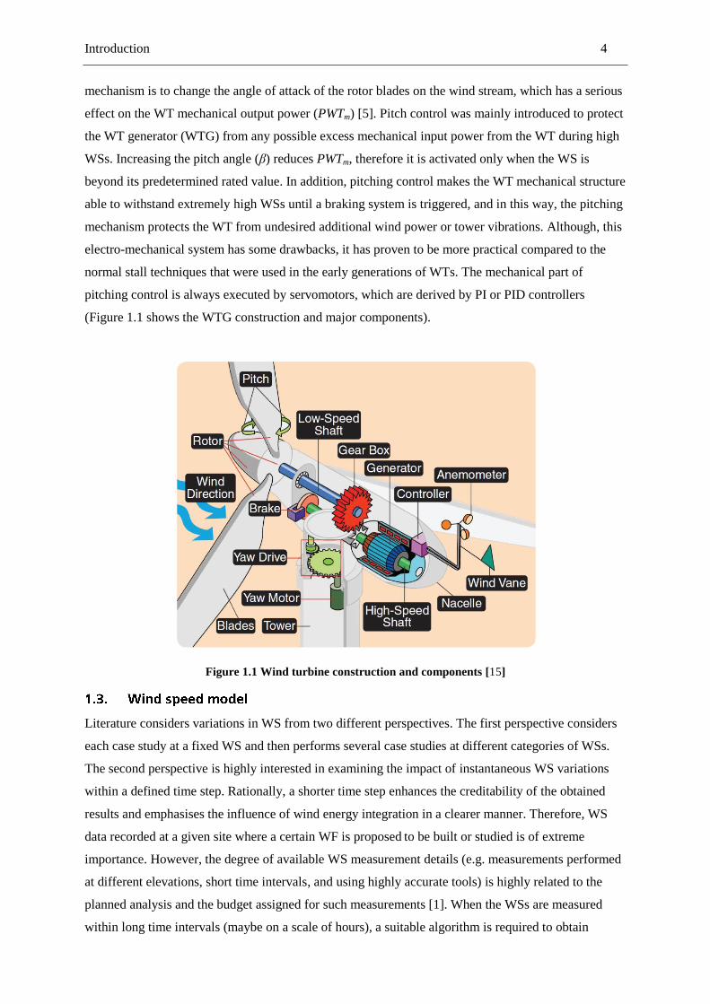
(Figure 1.1 shows the WTG construction and major components).
Figure 1.1 Wind turbine construction and components [15]
Literature considers variations in WS from two different perspectives. The first perspective considers
each case study at a fixed WS and then performs several case studies at different categories of WSs.
The second perspective is highly interested in examining the impact of instantaneous WS variations
within a defined time step. Rationally, a shorter time step enhances the creditability of the obtained
results and emphasises the influence of wind energy integration in a clearer manner. Therefore, WS
data recorded at a given site where a certain WF is proposed to be built or studied is of extreme
importance. However, the degree of available WS measurement details (e.g. measurements performed
at different elevations, short time intervals, and using highly accurate tools) is highly related to the
planned analysis and the budget assigned for such measurements [1]. When the WSs are measured
within long time intervals (maybe on a scale of hours), a suitable algorithm is required to obtain

Introduction 5
artificial arrays at a higher time resolution (for example 10 or 20 s), in order to fit with the power
system frequency performance analysis.
The other branch of WS variation modelling is related to its measurements inside a WF. In other
words, the magnitude of the WS at each WT inside a WF is the subject of continual debate. The most
dominant and simplified assumption ignores any deviations between WS values all over the WF area,
and represents the WF as a single WT with a rating that uses a combination of readings from all the
installed WTs. However, this assumption is only valid if all WTs are typical, and it causes a moderate
reduction in the accuracy of obtained results. In contrast, other studies focus on the shadowing and
wake effects and their impacts on the amount of instant power generated by a WF. Several methods
with complicated equations and approaches are available to consider such effects in simulating
integrated WFs through the prediction of incident WS values at each WT [16]. Generally, most
literature agrees that by considering only the annual average WS at a certain site for use in further
studies, a very poor approximation is rendered, yielding irrelevant results. This research work
therefore offers a detailed classification of available WSs at the WF concerned, and uses associated
case studies.
The main target of this research work is the elimination of any possible negative impacts on frequency
support, caused by WFs in replacing conventional generation units. Further, this work also focuses on
the ability to operate a WF in a similar manner to a conventional power plant and to predict the impact
of newly integrated wind energy on a given power system. Several models and algorithms are
proposed, and these are integrated and analysed to reach simple applicable methods with reduced
errors. The following steps are amalgamated:
WS data are gathered, examined, and filtered so that they are applicable to the
intended studies. WS generation mechanisms are applied at this stage to convert the
available WS data into artificial data with a higher time resolution.
The relation between stored KE in the WT rotating parts and WT speed is investigated.
The first support algorithm causes the WT to over-speed according to the
instantaneous WS, so that a certain amount of stored KE is maintained. This
extractable KE is utilized to deteriorate any frequency drops suffered by the power
system through an innovative support algorithm.
The electrical power control is involved in the second support algorithm. The WT is
de-loaded or decelerated or overloaded based on the WS conditions before and during
the frequency event. Numerical values of some of the parameters are pre-determined
and then fixed according to the WS nature and the installed WT types at the WF.
Introduction 6
These parameters master the proposed support algorithm in both operational modes,
namely, normal operational mode and support mode (i.e. when the frequency drops).
The two previous algorithms are compared with the standard MPT mode from the
point of view of performance curves and wasted energy. They are also compared to
the default de-loading technique widely offered in literature. Thereafter, a brief
discussion of the advantages and disadvantages of the support algorithms is
conducted.
A rough estimation is given for the annual wind energy expected from a certain
configuration of WFs and WTs. This assessment is conducted when the WTs are
operating in normal mode of the second support method. Proposed methodology
utilizes the chronological annual WS data at each WF site in the Egyptian case study.
Dispatching the power of WF during frequency events is considered to organize the
WTs contribution in mitigating frequency drops. In particular, the major task of
dispatching is to manage the switching process of WTs groups inside each WF,
between normal and support modes of the proposed algorithms. The dispatching
technique concedes fixed and variable parameters, such as the capacity of WF, and the
incident frequency drop and WS magnitude.
Finally, energy storage stations are integrated as an alternative for controlling WTs
using special support algorithms. A novel method is then proposed to estimate the
capacity of each storage bank connected to a particular WF. An appropriate approach
is presented for managing energy charging/discharging procedures.
It is worth mentioning that, there are minor and secondary objectives were also considered, as these
were essential in performing the previously stated foremost objectives. Some of these minor objectives
are described as a consequence of the related major objectives.
This thesis is composed of nine chapters. The following chapter presents an expanded technical survey
for the topics related to the performed research, and in particular in relation to the WT modelling and
control, ride through and support algorithms for frequency events, WSs data, and WFs‘ aggregation
methods. Chapters 3 and 4 present two different algorithms that ensure the positive contribution of the
WT in the curtailment of frequency excursions. Chapter 5 proposes a comparison between the offered
operation algorithms and standard operation from the point of view of wasted energy. Chapter 6
estimates the expected annual energy production of a selected group of WFs in Egypt, based on real
chronological data for load demand, conventional generation, and WS. Chapter 7 describes a novel

Introduction 7
method for dispatching power from WTs inside a WF during frequency drops. Clustering techniques
related to dispatching algorithms are also explained in this chapter. Chapter 8 then highlights storage
batteries as an alternative solution to the proposed support techniques. Finally, Chapter 9 concludes
and presents short recommendations based on the obtained results. In addition, it highlights future
topics for research.

Wind energy integration in power systems 8
The potential use of a substantial amount of wind energy in power systems poses numerous questions,
obstacles, and difficulties that require wise and rational dissection. This chapter highlights such basic
issues and emphasizes remediation in relation to this field of research addressed in recent literature. It
also addresses major topics related to wind energy generation and integration, and these are combined
with the objectives of this thesis.
Providing a feasible and realistic analysis for any component or system requires a robust, clear, and
detailed simulation model. The level of required details depends on the nature and aims of the planned
study, and therefore, certain parameters can be ignored to simplify computational efforts and shorten
the time involved. In addition, the model differs based on the simulated wind turbine type.
In general, there are three well-known types of WT, and these are classified according to their
capability of controlling the rotational speed [4]. However, some literature considers the doubly
outage induction generator (DOIG) to be an independent type; and hence classifies designs into four
types, as shown in Figure 2.1 [12].
Figure 2.1 Four principal concepts used in WTs [12]
a) Fixed speed squirrel cage induction generator b) Partial variable speed WT with variable rotor
resistance
c) Double Fed induction generator d) Full rated permanent magnet generator
Initial trials in modern WT fabrication produced the squirrel cage induction generator (SCIG) (Type 1)
which contained a simplified control algorithm. However, compared to other types of WTs, it wastes
more wind energy because it has a fixed operation point and the WT rotational speed is uncontrollable,

Wind energy integration in power systems 9
and thus, it is unable to track the continuous variations in WS. It relies on a connected capacitor bank
to energize the WT (fulfil the machine‘s reactive power requirements), and maintain connection
voltage stability during faults. Additionally, the ratings of the WTG units are limited to hundreds of
kilowatts, and it also has certain problems in relation to maintenance and operation. The current
dominant and most applicable technology is Type 3. The major advantage of Type 3 is its capability
for the tracking optimum operation conditions at each WS. As a further explanation, a compact review
of each WT‘s operational theory is presented.
The physical idea behind a WT depends on converting wind kinetic energy into electrical energy
through a WT generator. The output mechanical power (PWTm) from the WT is evaluated using (2.1):
31( , ) A
2m pPWT C WS (2.1)
The air density (ρ) used is 1.225 kg/m3 [1], Cp is the coefficient of performance, λ is the tip speed ratio
calculated using (2.2), β is the pitch angle and A is the WT rotor swept area in m2:
R
WS
(2.2)
The evaluation of Cp depends on the aerodynamic characteristics‘ of the airfoil of blades. The airfoil
design distributes the lift and drag forces implied by wind on the blade, thus the amount of extractable
wind energy is determined. However, the maximum possible value for Cp is 16/27 as proved by Betz‘
law [1]. According to the previous equations, PWTm variations directly affect generator output.
However, there are two main parameters that control PWTm, namely, λ and β. The control of λ is
achieved through Ѡ, and control of β is executed using electro-mechanical pitch angle controllers, if
the WT is equipped with such a facility [5]. Both parameters are coherently controlled to make Cp
follows its optimum pre-determined value (Cp-optimum), which differs from one WT to another
depending on several factors, for example the size and aerodynamic profile of the installed blades (i.e.,
default Cp-optimum value is 0.48). The function that describes the relation between the Cp, λ and β, is
considered to be an empirical formula with a certain number of coefficients, and it is totally dependent
on the rotor blades design and WT characteristics. Equation (2.3) represents a widely applied form for
this function in literature, where c1 to c6, besides a and b are the related coefficients. Numerical values
for these coefficients are simulated in the GE-1.5 MW WT (GE-77) generic model built in MATLAB
Simulink power library [17]. A 3-D visualization for the Cp equation of GE-1.5 MW is depicted in
Figure 2.2, where the Cp-optimum is 0.48, and it doesn‘t exceed the maximum theoretical value, namely,
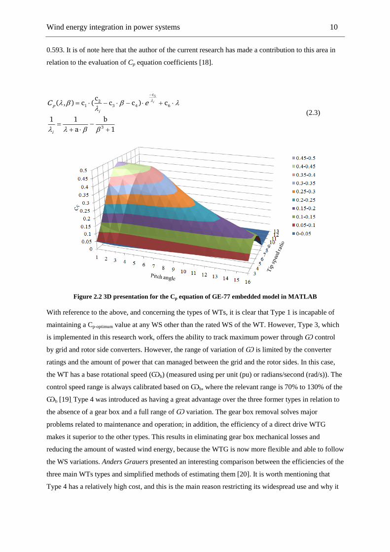
Wind energy integration in power systems 10
0.593. It is of note here that the author of the current research has made a contribution to this area in
relation to the evaluation of Cp equation coefficients [18].
5c
21 3 4 6
3
c( , ) c ( c c ) c
1 1 b
a 1
i
p
i
i
C e
(2.3)
Figure 2.2 3D presentation for the Cp equation of GE-77 embedded model in MATLAB
With reference to the above, and concerning the types of WTs, it is clear that Type 1 is incapable of
maintaining a Cp-optimum value at any WS other than the rated WS of the WT. However, Type 3, which
is implemented in this research work, offers the ability to track maximum power through Ѡ control
by grid and rotor side converters. However, the range of variation of Ѡ is limited by the converter
ratings and the amount of power that can managed between the grid and the rotor sides. In this case,
the WT has a base rotational speed (Ѡb) (measured using per unit (pu) or radians/second (rad/s)). The
control speed range is always calibrated based on Ѡb, where the relevant range is 70% to 130% of the
Ѡb [19]. Type 4 was introduced as having a great advantage over the three former types in relation to
the absence of a gear box and a full range of Ѡ variation. The gear box removal solves major
problems related to maintenance and operation; in addition, the efficiency of a direct drive WTG
makes it superior to the other types. This results in eliminating gear box mechanical losses and
reducing the amount of wasted wind energy, because the WTG is now more flexible and able to follow
the WS variations. Anders Grauers presented an interesting comparison between the efficiencies of the
three main WTs types and simplified methods of estimating them [20]. It is worth mentioning that
Type 4 has a relatively high cost, and this is the main reason restricting its widespread use and why it

Wind energy integration in power systems 11
is only installed in large and highly rated WTs (e.g. Enercon-101 3.4 MW [21]). The market shares of
the four major types of WTs in 2010 are depicted in Figure 2.3 [22].
Figure 2.3 Wind power capacity market share of each WT technology
Literature divides the WT model into four sub-models, the complexity and level of considered details
depend on the study field employing the models. The four sub-models are the WT aerodynamic
model, the shaft connecting WT to generator (i.e., drive train) or the shaft model, the generator model,
and the pitch angle electro-mechanical controller model. The type of WT only affects the generator
model and the method by which this generator is controlled when it is connected to the grid [7]. The
WT aerodynamic model is usually presented by using the Cp equation previously explained in Section
(2.1.1), where this model has three inputs, namely, Ѡ, β, and WS, as well as one output, PWTm. The
shaft model is mathematically presented by a two-mass, as shown in Figure 2.4 or a single mass
model. The shaft model receives two inputs (i.e., PWTm from the aerodynamic model and Ѡ), delivers
turbine power, and is essential for use with fixed speed WTGs, but can be ignored in variable speed
WTGs (however, it depends on the aims of the study). Disregarding the shaft model in the overall
integrated simulated model was a valid assumption in [23], where the method presented describes the
connection of a permanent magnet synchronous generator (PMSG) WT through a DC link controlled
by a thyristor converter. Although the PMSG is a fixed speed generator, the presence of the DC power
electronics-controlled link ensures that the role of shaft inertia is very minor. A third sub-model is
constructed to control the pitch angle, and functions using two parts, the proportional integral (PI)
controller and the servomotor. The servomotor model is well known and its design is predominantly
similar in all literature. However, several designs and methodologies have been proposed for installed
PI controllers. Initially, a pitch controller was installed in WTGs to offer an alternative to the normal
stalling mechanism, and to extend the operation range of the WT in certain WSs. To understand the
possible uses of a pitch controller, it is necessary to look at the WT output power curve vs. WS, as in
Figure 2.5. As an illustration, PWTm continuously increases with an increase of WS until it reaches
WT rated WS (WSr). Beyond this WS, the WT is able to produce a PWTm higher than the rated power
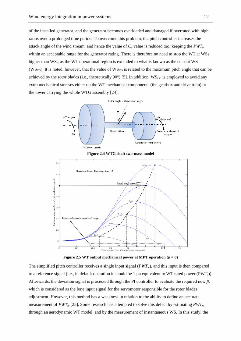
Wind energy integration in power systems 12
of the installed generator, and the generator becomes overloaded and damaged if overrated with high
ratios over a prolonged time period. To overcome this problem, the pitch controller increases the
attack angle of the wind stream, and hence the value of Cp value is reduced too, keeping the PWTm
within an acceptable range for the generator rating. There is therefore no need to stop the WT at WSs
higher than WSr, as the WT operational region is extended to what is known as the cut-out WS
(WSCO). It is noted, however, that the value of WSCO is related to the maximum pitch angle that can be
achieved by the rotor blades (i.e., theoretically 90°) [5]. In addition, WSCO is employed to avoid any
extra mechanical stresses either on the WT mechanical components (the gearbox and drive train) or
the tower carrying the whole WTG assembly [24].
Figure 2.4 WTG shaft two-mass model
Figure 2.5 WT output mechanical power at MPT operation (β = 0)
The simplified pitch controller receives a single input signal (PWTm), and this input is then compared
to a reference signal (i.e., in default operation it should be 1 pu equivalent to WT rated power (PWTr)).
Afterwards, the deviation signal is processed through the PI controller to evaluate the required new β,
which is considered as the lone input signal for the servomotor responsible for the rotor blades‘
adjustment. However, this method has a weakness in relation to the ability to define an accurate
measurement of PWTm [25]. Some research has attempted to solve this defect by estimating PWTm
through an aerodynamic WT model, and by the measurement of instantaneous WS. In this study, the
Wind energy integration in power systems 13
dependence of the estimation of β on PWTm proved to be inaccurate, and produced an undesired
oscillatory response in the WT electrical output power (PWTe), as discussed later in Chapter 6 [26].
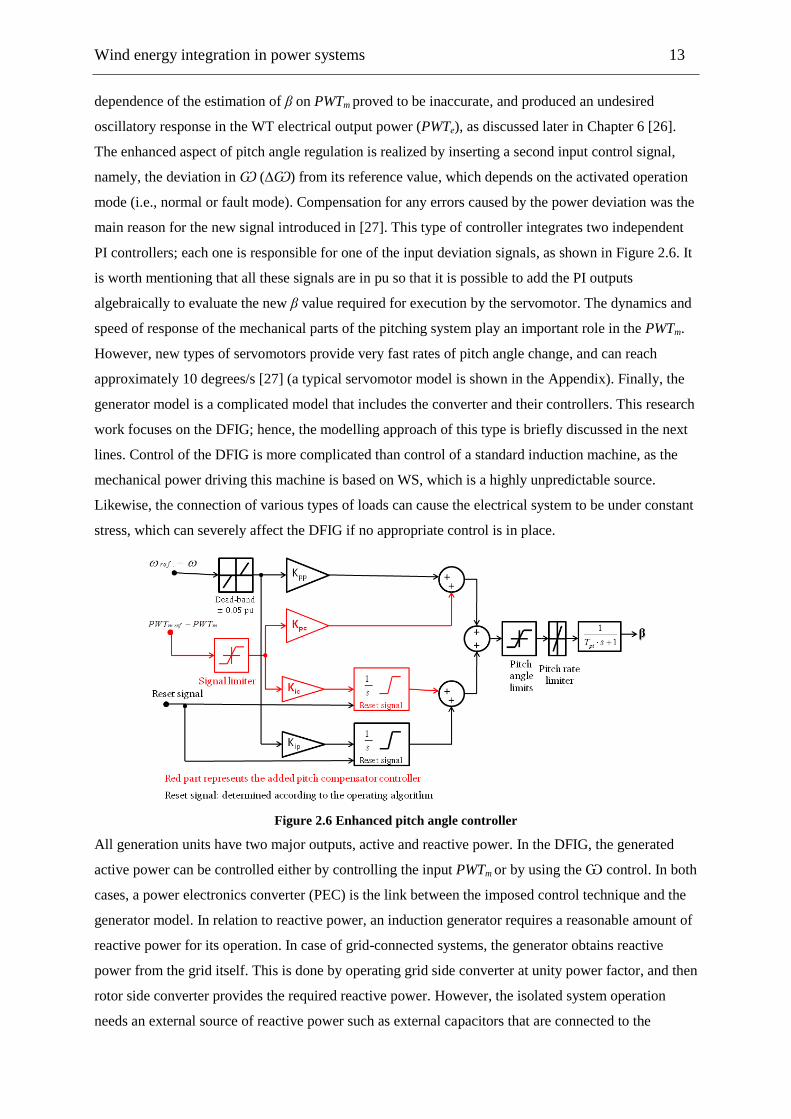
The enhanced aspect of pitch angle regulation is realized by inserting a second input control signal,
namely, the deviation in Ѡ (∆Ѡ) from its reference value, which depends on the activated operation
mode (i.e., normal or fault mode). Compensation for any errors caused by the power deviation was the
main reason for the new signal introduced in [27]. This type of controller integrates two independent
PI controllers; each one is responsible for one of the input deviation signals, as shown in Figure 2.6. It
is worth mentioning that all these signals are in pu so that it is possible to add the PI outputs
algebraically to evaluate the new β value required for execution by the servomotor. The dynamics and
speed of response of the mechanical parts of the pitching system play an important role in the PWTm.
However, new types of servomotors provide very fast rates of pitch angle change, and can reach
approximately 10 degrees/s [27] (a typical servomotor model is shown in the Appendix). Finally, the
generator model is a complicated model that includes the converter and their controllers. This research
work focuses on the DFIG; hence, the modelling approach of this type is briefly discussed in the next
lines. Control of the DFIG is more complicated than control of a standard induction machine, as the
mechanical power driving this machine is based on WS, which is a highly unpredictable source.
Likewise, the connection of various types of loads can cause the electrical system to be under constant
stress, which can severely affect the DFIG if no appropriate control is in place.
Figure 2.6 Enhanced pitch angle controller
All generation units have two major outputs, active and reactive power. In the DFIG, the generated
active power can be controlled either by controlling the input PWTm or by using the Ѡ control. In both
cases, a power electronics converter (PEC) is the link between the imposed control technique and the
generator model. In relation to reactive power, an induction generator requires a reasonable amount of
reactive power for its operation. In case of grid-connected systems, the generator obtains reactive
power from the grid itself. This is done by operating grid side converter at unity power factor, and then
rotor side converter provides the required reactive power. However, the isolated system operation
needs an external source of reactive power such as external capacitors that are connected to the
Wind energy integration in power systems 14
machine rotor through PEC. In special cases, capacitors are replaced by an external source (i.e.,
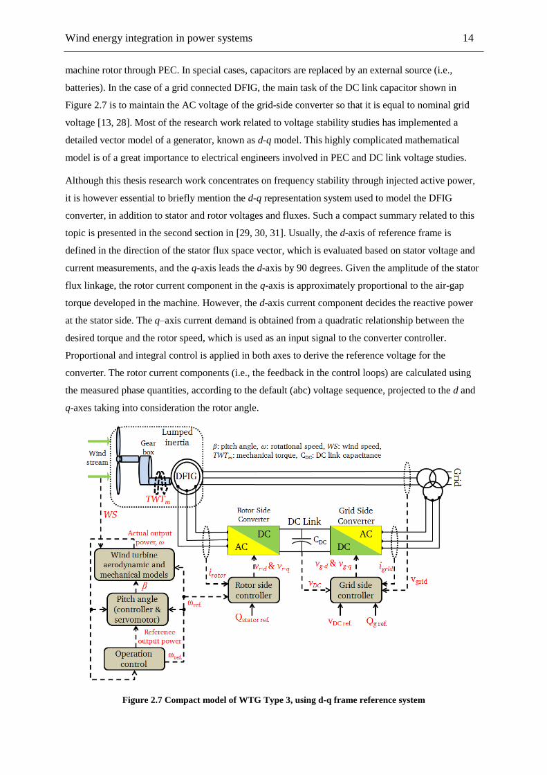
batteries). In the case of a grid connected DFIG, the main task of the DC link capacitor shown in
Figure 2.7 is to maintain the AC voltage of the grid-side converter so that it is equal to nominal grid
voltage [13, 28]. Most of the research work related to voltage stability studies has implemented a
detailed vector model of a generator, known as d-q model. This highly complicated mathematical
model is of a great importance to electrical engineers involved in PEC and DC link voltage studies.
Although this thesis research work concentrates on frequency stability through injected active power,
it is however essential to briefly mention the d-q representation system used to model the DFIG
converter, in addition to stator and rotor voltages and fluxes. Such a compact summary related to this
topic is presented in the second section in [29, 30, 31]. Usually, the d-axis of reference frame is
defined in the direction of the stator flux space vector, which is evaluated based on stator voltage and
current measurements, and the q-axis leads the d-axis by 90 degrees. Given the amplitude of the stator
flux linkage, the rotor current component in the q-axis is approximately proportional to the air-gap
torque developed in the machine. However, the d-axis current component decides the reactive power
at the stator side. The q–axis current demand is obtained from a quadratic relationship between the
desired torque and the rotor speed, which is used as an input signal to the converter controller.
Proportional and integral control is applied in both axes to derive the reference voltage for the
converter. The rotor current components (i.e., the feedback in the control loops) are calculated using
the measured phase quantities, according to the default (abc) voltage sequence, projected to the d and
q-axes taking into consideration the rotor angle.
Figure 2.7 Compact model of WTG Type 3, using d-q frame reference system
Wind energy integration in power systems 15
An innovative criterion presented by Padrón, applies the Newton Raphson iterative method to propose
two possible WTG models for load flow analysis, namely the active-reactive power bus (PQ) and the
active power-voltage bus (PV) [32]. In such way, a WTG, or even a complete WF, can be treated in a
similar way to a conventional generator. The main idea is based on assuming that the WT or WF bus is
the only unknown bus in the system, whereas the bus type differs based on the implemented method.
Thus PWTm equals P, and the voltage vector is then estimated using an iterative method (in the case of
PQ), and likewise Q and the voltage angle are estimated in the case of the PV bus. This work has
considerable additional strength in that it does not use the complicated d-q reference frame. However,
if more than one WF is connected, these two methods have drawbacks concerning WS prediction
complications and WS measurement accuracy. In addition, the WS is calculated using back
substitution according to required aggregated power. In other words, the load flow analysis determines
the optimum incident WS to satisfy the system requirements. This concept is hard to apply in dynamic
analysis, but is practical and simplified when it comes to steady state load flow analysis and DFIG
initialization.
Based on the previous brief background, the merits of DFIG can be summarized in four points: 1) it
delivers reduced wasted wind energy; 2) the mechanical loads are less and it delivers a simpler pitch
control; 3) the controllability of both active and reactive power to achieve near-independency; and 4)
oscillations in output power are mitigated.
This section reviews the main WTG operational theories widely offered in literature. The design of
such operational methodologies depends on the desired aims, or on the nature of the problem to be
solved. Categories of operational methodologies can be summarized by the use of three general
approaches: maximum power tracking, low voltage ride through algorithms, and frequency drops ride
through and support algorithms. However, it is extremely difficult to achieve these three targets
together with a level of adequacy; hence, a compromise is made between them to reach an acceptable
solution matching the prerequisites of the involved power system. Because this thesis is oriented to
solve frequency drops problems, a separate subsection discusses this approach (Section 2.3).
The current dominant operation algorithm for integrated WTGs in power systems aims to minimize
any wasted wind energy. Therefore, this operational mode adjusts the controllable parameters in WTG
to match the intermittent nature of the WS. In fact, this operation algorithm tries to provide Ѡ, which
achieves Cp-optimum, and in turn maximum values of PWTm [6]. Applying this technique produces an
operation curve, which shows a set of different operational points of the WT concerned at WSs less
than WSr, as shown in Figure 2.5. This operational mode implies a zero degree pitch angle because all
operational points are below WSr. In this case, the controller is responsible for providing the reference
rotational speed signal and the related PWTm fluctuations, which act as an input to the rotor side
controller, as described in Figure 2.8. Meng made an influential modification in the MPT curve to
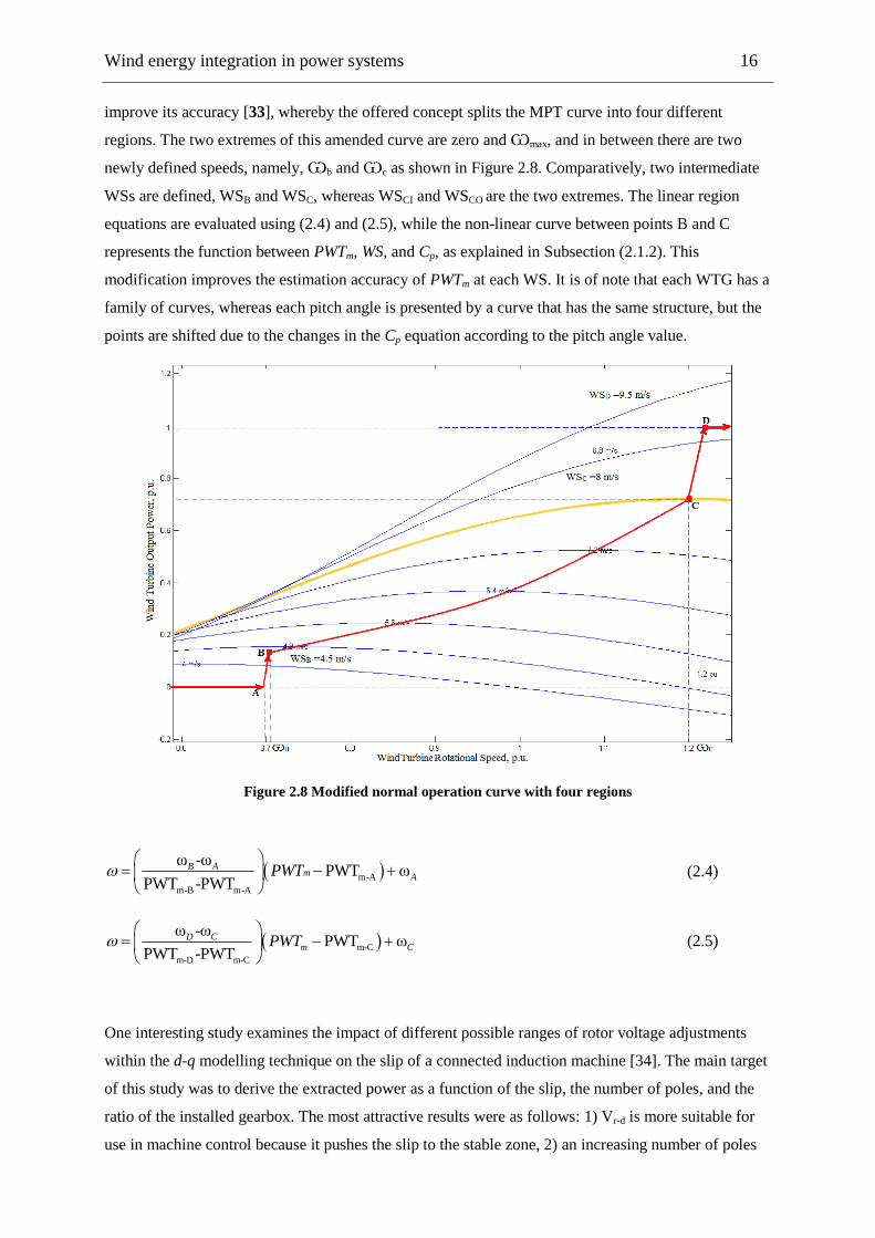
Wind energy integration in power systems 16
improve its accuracy [33], whereby the offered concept splits the MPT curve into four different
regions. The two extremes of this amended curve are zero and Ѡmax, and in between there are two
newly defined speeds, namely, Ѡb and Ѡc as shown in Figure 2.8. Comparatively, two intermediate
WSs are defined, WSB and WSC, whereas WSCI and WSCO are the two extremes. The linear region
equations are evaluated using (2.4) and (2.5), while the non-linear curve between points B and C
represents the function between PWTm, WS, and Cp, as explained in Subsection (2.1.2). This
modification improves the estimation accuracy of PWTm at each WS. It is of note that each WTG has a
family of curves, whereas each pitch angle is presented by a curve that has the same structure, but the
points are shifted due to the changes in the Cp equation according to the pitch angle value.
Figure 2.8 Modified normal operation curve with four regions
m-A
m-B m-A
ω -ωPWT ω
PWT -PWT
B Am APWT
(2.4)
m-C
m-D m-C
ω -ωPWT ω
PWT -PWT
D Cm CPWT
(2.5)
One interesting study examines the impact of different possible ranges of rotor voltage adjustments
within the d-q modelling technique on the slip of a connected induction machine [34]. The main target
of this study was to derive the extracted power as a function of the slip, the number of poles, and the
ratio of the installed gearbox. The most attractive results were as follows: 1) Vr-d is more suitable for
use in machine control because it pushes the slip to the stable zone, 2) an increasing number of poles

Wind energy integration in power systems 17
leads to a wider stable operational range for the slip, and 3) increasing the gearbox ratio displaces the
slip from the sub-synchronous region to the super-synchronous region. An advanced current control
method is proposed by Hu, where both sides of the DFIG converter currents are controlled to mitigate
third order harmonics in the WT generated electromagnetic torque during unbalanced grid voltage
conditions [30]. This proposes a novel control scheme consisting of a proportional controller and a
harmonic resonant regulator tuned at grid frequency. However, this research track is specialized for
detailed control issues and their integration with PECs.
In relation to the wide research presented in this chapter, this section is mostly related to the core of
the proposed algorithms and the associated research work described in this thesis. The ride-through
algorithms are classified into two categories; low voltage and frequency drop ride-through algorithms
(LVRT and FDRT respectively). Using an analogy with conventional units, LVRT depend on special
reactive power and DC link voltage control techniques [35], whereas, FDRT build on controlling the
PWTm, mechanical torque (TWTm) and/or the reference electrical power signal fed to the converter-
generator controller (PWTe). Frequency support algorithms are also related to the control of active
power generated by a WT during frequency excursions. The major target of these algorithms is to
provide an extra amount of active power from WTs in the case of frequency events, to accelerate the
frequency drop elimination process. The next two subsections summarize the latest concepts in
relation to LVRT and FDRT algorithms offered in literature. However, the focus is centred on
frequency support, as this thesis is directed towards this research point.
–
The possibility of a WT disconnecting under voltage drops depends on the location of the fault with
respect to the point of common coupling (PCC), the drop duration, type and severity, the method of
reactive power compensation, and the control algorithm of the WT. Most of the proposed solutions
wander in the orbit of compensation or dissipation of the missing or extra KE caused by the voltage
drop or rise. This can be executed by the wise control of rotor side currents, WT rotational speed, and
the pitch angle [36]. LVRT research work is interested in detailed dynamic modelling for WTs and
WFs; hence, the d-q reference frame is implemented. The DFIG has a unique advantage concerning its
ability to control active and reactive power almost independently, which facilitates the task of
providing excess reactive power during voltage dips [8]. The rotor current is controlled in such a way
to reduce any DC link voltage ripples, especially during system voltage events [29]. However, the
DFIG provides no support to mitigate the voltage drops, but the negative impact of wind energy
integration is reduced. Another study proposed novel methods of connecting WTs to the grid. This
method improves the voltage imbalance compensation, as voltage is injected in series with the
transmission line to limit the fault currents as well as to balance the voltages [37]. The modifications
are implied only on the grid side converter; thereupon, it is connected in series instead of parallel
Wind energy integration in power systems 18
installation. Additionally, the three-phase converter is replaced by three single-phase converters. Each
converter is responsible for a certain regulating task, for example, the phase ‗A‘ converter
compensates for the voltage imbalance. Generally, when a short-term low-voltage fault occurs, the
sudden imbalance between wind energy and injected electrical energy leads to transient excessive
currents in the rotor and stator circuits. Therefore, suppressing the over-currents in the rotor and stator
circuits should reduce the imbalanced energy flowing through the DFIG system. To achieve this
suppression, the excess KE provided by the WT can be dissipated by accelerating the WT rotational
speed by controlling the rotor side converter [28]. Similar work is applied to PMSG as well as DFIG
WFs, to maintain rotor currents and DC link voltage levels [38]. The major change is that it reduces
the active power fed by the WTG proportional to the incident voltage dip. Far from control algorithms,
an integrated component called crowbar protection could be used to enable survival of the WT through
such an event. A simplified explanation of the role of the crowbar, accompanied by a detailed case
study using a hypothetical test system, is described in [39]. It is of note that voltage stability studies
are not able to ignore transmission lines and transformers models, as shown in the considered case
study in [39]. This highlights their influential impact on the accuracy and relevance of the obtained
results, as they affect the reactive power flow throughout the whole system. This work emphasizes the
role of the crowbar in causing the DFIG to behave as a conventional SCIG, when its controllability is
temporarily lost. In the same vein, crowbar resistance is operated for a shorter time in the proposed
strategy by [40], so that there is a shorter interval where there is no control on the DFIG. In addition,
the energy losses in the crowbar resistors are mitigated. The proposed strategy is based on increasing
crowbar resistors to a certain value that is a multiple of rotor equivalent resistance. The compensation
for the short crowbar connection time is made through demagnetization of the stator; hence, the
current oscillations are attenuated. A simple demagnetization method is applied through setting the
reference signal of the rotor current‘s two components in the d-q frame to zero. However, this work is
highly oriented to power electronics and machine theory, and is therefore very complicated to
integrate with expanded power system analysis. In addition to the above, the crowbar is triggered for
an interval 50% less than its usual duration, without adding any external devices [41]. In usual
operation, the crowbar is released after a certain fixed time, where half of this time is implied to
guarantee that the reference signals of the rotor side converter settle down to acceptable values. The
research work in [41] eliminated this duration by applying a predetermined reference signal to the
rotor side converter, taking into consideration that these signal values yield a reasonable power factor.
However, these imposed values are provisional until real values are obtained; nevertheless, the earlier
re-connection of rotor side converter is achieved. In the light of previous discussion, the aims of any
LVRT can be summarized as follows: 1) to minimize the voltage drop at the generator through
demagnetization techniques, 2) to divert or negate any rotor overrated currents to avoid damage to the
converter, 3) to produce appropriate power during faults where the DFIG controller limits the rate at

Wind energy integration in power systems 19
which apparent power control can be restored during fault initiation and recovery. In such a way,
DFIG compliance with the grid-code is fulfilled.
At present, WFs do not play a fundamental role in eliminating system frequency events, as most grid
codes do not force them to provide any support during frequency excursions. However, in order to
allow high levels of wind power penetration, system operators (SOs) will eventually require wind
generation to have frequency control capabilities in future updated codes [42]. For example, SOs in
Ireland are attempting to solve operational and infrastructure obstacles so that WFs cover 37% of the
electricity demand. The outcomes of the 2010 Facilitation of Renewable (FoR) studies predicts deficits
in system performance capability in terms of frequency control by the year 2020, as a greater number
of the non-synchronous generation become integrated in the system. In terms of frequency control,
analysis has shown that projected levels of synchronous inertia that will be available in 2020 will be
less than amounts needed to meet system requirements.
Frequency control becomes more challenging at high wind energy penetration levels. As an
illustration, the rate of change of frequency (ROCOF) protection relays shut down WTs under certain
scenarios. Investigations are currently under way to either replace ROCOF protection relays on the
distribution networks with alternative protection schemes or to increase ROCOF thresholds [43].
However, the main challenge is related to the supportive contribution of WFs during frequency events.
Positive frequency deviations do not cause a critical influence, as they are always the result of a
mismatch between generation and load demand where the generation rises suddenly beyond required
load. In such scenarios, a portion from the WFs is disconnected according to the system status, and the
WFs reconnection is then decided based on the system‘s new stable operation conditions. These
manoeuvre methods have also been investigated to determine the optimum amount of disconnected
wind energy according to the characteristics of frequency overshoot events and other factors [6].
However, when a system suffers a frequency drop, WFs are requested to compensate the deficit
between generation and demand, similar to conventional generation. Conventional generators have
governor controllers at different levels of complication and accuracy, and these provide a control
signal to the source of mechanical power, the turbine, which in turn drives the synchronous generator
shaft. For example, in steam generators, the most dominant type in conventional generation, the
mechanical power is determined according to the flow rate of steam exerted on the turbines vanes.
Thus, the governor controls the valve opening, such that the required flow rate of steam is injected to
the turbine [10]. The governor operation is based on two major signals: the electrical power demand
and the instantaneous frequency deviation (∆f). The ∆f signal is responsible for the generation unit
dynamic response in case of frequency excursions, whereas the droop parameter makes links between
the amounts of increase/decrease in generated power according to the incident drop/rise in frequency
deviation. The numerical value of droop ranges from 5% to 10%, for example if droop = 5% this
means that for each 1 Hz change in frequency, the unit output changes from its capacity by 5% [44].
Wind energy integration in power systems 20
It is an essential prerequisite to find an acceptable method that guarantees the positive contribution
from WFs during frequency drops, especially when WFs replace conventional units and penetrate
power systems at high levels. The intermittent nature of WSs is the major obstacle facing electrical
power engineers in this field, and in comparison with fuel used in conventional units, WS is
unpredictable and cannot be controlled. For example, in a steam plant, the flow of steam is available
and controllable at all times, as long as the fossil fuel used to produce the steam is available. Hence,
the SOs perform previews of system operation, and expect certain reactions from these units during
fault events. Such an advantage is completely absent in the case of WFs, because they completely
depend on the coincidence between frequency drops and the nature of WS during the drops. For
example, if a WTG is connected to a standard governor, such as the one connected to a conventional
unit, which then orders a certain output from the WT, but the WS is insufficient to satisfy this
reference output power, it is necessary to ascertain feasible solutions for such a dilemma.
Another challenge is related to the reduced inertia of power systems after the installation of WFs.
Extended research has proven that grid inertia in seconds (H) is notably affected by the integration of
WTGs. This negative impact is more remarkable in cases of variable speed WTGs [45]. The
interpretation of this phenomenon depends on a comparison between synchronous generators used in
conventional units and variable speed WTGs, whereas the fast response of WTGs, caused by the great
developments in upgrading the speed of PECs technologies to milliseconds, makes the WTGs inertia-
less [46]. This problem is partially overcome by using fixed speed WTs, but this reduces the harvested
wind energy and WT efficiency [47]. It is of note that the inertia of conventional generators ranges
from 3 s to 8 s, based on generator type and capacity [48]. The solutions offered in literature are
concentrated in two directions: 1) running the WTG in an analogous manner to conventional units by
defining a special droop controller [49]; 2) imposing virtual inertia to the WTG through unique control
algorithms [50]; and 3) utilizing several types of storage banks to smooth WFs output, using the
available stored energy. The storage process occurs when the generated wind energy is rejected by the
system during trough load periods [51]. Expanded explanations and discussion concerning these
solutions are presented within the next related chapters. The implemented concept to simulate the
frequency response of the test systems in the next chapters is based on the aggregate bus criterion as
explained in [52] [53]. The illustrative Figure 2.9 highlights the major four sub-models, namely, the
conventional generation aggregate unit(s), the dynamic load, WF(s) and the system aggregate inertia.
Actually, the most effective component of a conventional generation unit on frequency are the
controller that sets reference power, the governor and the turbine as discussed in [52] [53]. The load
dynamics are presented by load dependent and independent components with respect to frequency
variations. The WF is composed from four major blocks, firstly, the operation algorithm that is
responsible for setting ω, reference output power and pitch angle, as well as some special signals
which differ from one algorithm to another. Secondly, the aerodynamics which determines how much
mechanical power is extracted from wind power, thirdly, the mechanical model represented by Euler‘s
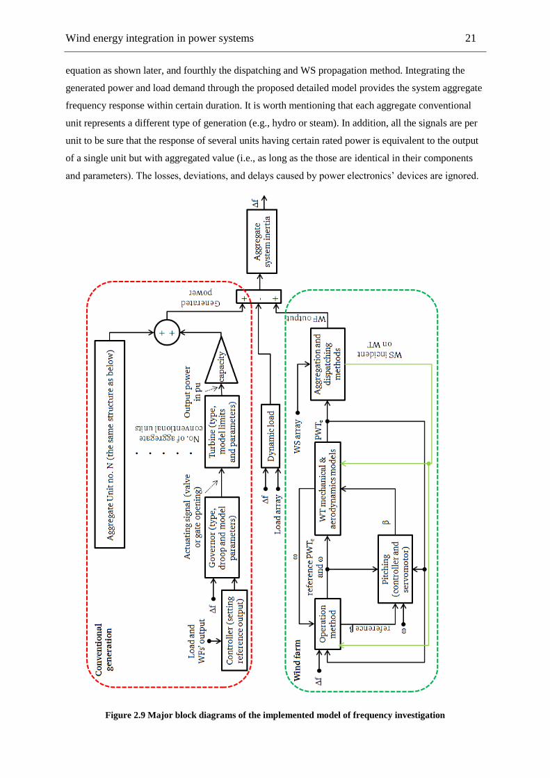
Wind energy integration in power systems 21
equation as shown later, and fourthly the dispatching and WS propagation method. Integrating the
generated power and load demand through the proposed detailed model provides the system aggregate
frequency response within certain duration. It is worth mentioning that each aggregate conventional
unit represents a different type of generation (e.g., hydro or steam). In addition, all the signals are per
unit to be sure that the response of several units having certain rated power is equivalent to the output
of a single unit but with aggregated value (i.e., as long as the those are identical in their components
and parameters). The losses, deviations, and delays caused by power electronics‘ devices are ignored.
Figure 2.9 Major block diagrams of the implemented model of frequency investigation
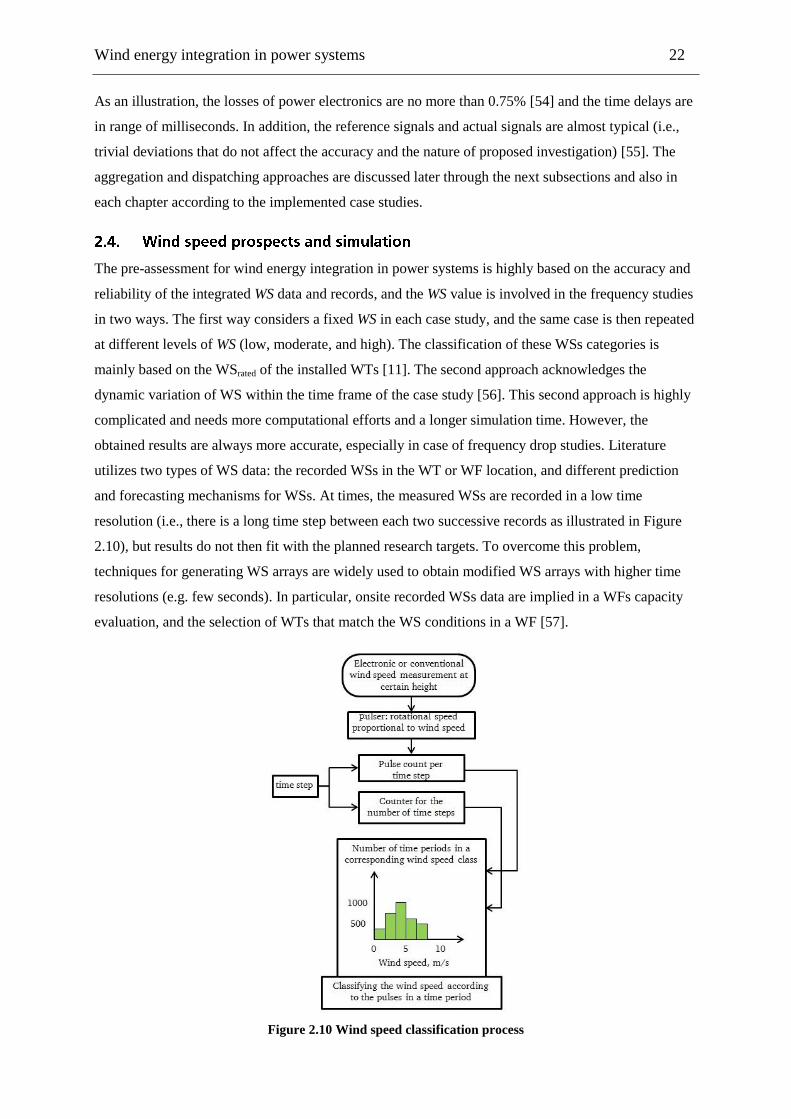
Wind energy integration in power systems 22
As an illustration, the losses of power electronics are no more than 0.75% [54] and the time delays are
in range of milliseconds. In addition, the reference signals and actual signals are almost typical (i.e.,
trivial deviations that do not affect the accuracy and the nature of proposed investigation) [55]. The
aggregation and dispatching approaches are discussed later through the next subsections and also in
each chapter according to the implemented case studies.
The pre-assessment for wind energy integration in power systems is highly based on the accuracy and
reliability of the integrated WS data and records, and the WS value is involved in the frequency studies
in two ways. The first way considers a fixed WS in each case study, and the same case is then repeated
at different levels of WS (low, moderate, and high). The classification of these WSs categories is
mainly based on the WSrated of the installed WTs [11]. The second approach acknowledges the
dynamic variation of WS within the time frame of the case study [56]. This second approach is highly
complicated and needs more computational efforts and a longer simulation time. However, the
obtained results are always more accurate, especially in case of frequency drop studies. Literature
utilizes two types of WS data: the recorded WSs in the WT or WF location, and different prediction
and forecasting mechanisms for WSs. At times, the measured WSs are recorded in a low time
resolution (i.e., there is a long time step between each two successive records as illustrated in Figure
2.10), but results do not then fit with the planned research targets. To overcome this problem,
techniques for generating WS arrays are widely used to obtain modified WS arrays with higher time
resolutions (e.g. few seconds). In particular, onsite recorded WSs data are implied in a WFs capacity
evaluation, and the selection of WTs that match the WS conditions in a WF [57].
Figure 2.10 Wind speed classification process
Wind energy integration in power systems 23
Most research work interested in the reliability optimization of power system expansion tends to
implement the Wei-bull probability distribution of WS. This distribution describes the occurrence
probability of several categories of WS within a year. However, these studies require fresh WS data
and their results are only guaranteed for a short time period [58]. Novel and comprehensive efforts in
the field of wind power assessment based on WS time series prediction are offered in [59], where four
different methods are investigated to predict the output power of a WF composed of 100 WTs. Firstly,
a suitable 10 min WS series and an applied method were selected to forecast multiples of WS series at
a point 10 min into the future. The same procedure was repeated for an hourly time series, and as
expected, it proved to be less accurate. A tangible idea is performed using neural networks, as
presented in [60]. The applied neural network was moderately complicated with five input delays, one
hidden layer, five neurons in the hidden layer, and 100 training iterations. However, neural network
integration is out of the scope of the research work presented in this thesis, but is considered as a topic
for possible future work. Far from planning and previewing system performance before actual wind
energy integration, other efforts have been directed to exploiting WS prediction techniques in the
curtailment of WTs output power fluctuations [61]. The wind model used was a stochastic model from
a certain block set for Simulink, which uses a white noise generator and filters to represent the main
wind source, and another noise generator and filter for turbine tower shadowing effects. Additionally,
WS is assumed to vary between one WT and another at the same instant, but this point has greater
relevance to the information presented in the following section.
It is initially important to highlight the motives for investigating this issue. As previously stated, WS is
the ‗fuel‘ that runs a WTG; hence, all related concepts and facts pertaining to WS need to be covered
and studied to achieve acceptable results in previewing, operating, and simulating WFs. It is
impossible to say that concurrent WSs are identical in two different locations, even if such locations
are only hundreds of meters apart. Therefore, claiming that all the WTs inside one WF facing the same
WS magnitude and direction is a special approximate assumption. In addition, towers with a WTG
assembly cause shadowing effects. These effects reduce the WS during its propagation in the WF, in
comparison with the WS magnitude that reaches the first WTs at the WF. The influence of shadowing
and wake effects is related to several parameters: tower height, land roughness coefficient (kw), and
the spacing between two successive WTs that impede the free WS stream [16, 62]. It is of note that
these effects impose a time delay between the different streams of WSs propagating inside the same
WF. For example, the WS at the first WT that is facing the initial wind stream, which reaches the WF,
is ahead in time of the wind stream projected on the blades of the last row of WTs. This time delay
depends on the spacing between the rows of WTs, and the wind stream‘s initial WS just before passing
through the WF [63]. Electrical power engineers have therefore been encouraged to propose a wide
spectrum of solutions for the best modelling approach of a complete WF.

Wind energy integration in power systems 24
The level of complexity and details that are integrated depends on several factors, including 1) the
target of the study implementing such a model; 2) the data available in relation to the WF‘s
geographical layout and terrain nature; 3) the WTs numbers, and types; 4) the distribution of WTs
inside the WF (are they spread in a regular manner or spread according to the terrain); and 5) the
degree of accuracy and time resolution of WS records, as well as the number of points inside the WF
where WSs arrays are recorded. Generally, the most accurate method to model a WF is to include a
single independent model for each installed WT and the corresponding WS stream incident upon it.
Thereafter, the overall output of the WF is the algebraic summation of all the installed WTs per each
time step. This method requires huge computational efforts and time, besides large data storage to
perform such simulations, especially if tens of WFs are considered and each one is composed of
hundreds of WTs.
Aggregating the WF as a single rescaled WT is the simplest and most widely applied method [5]. The
aggregated WF rating equals the name plate rating of a single WT multiplied by the number of
connected WTs, and the WTG model is then typical of a single unit model. However, this method is
only valid when all the installed WTs are of the same type and are made by the same manufacturer.
Otherwise, perceptible deviations and errors would arise between the aggregated model and the actual
performance of the simulated WF. The level of detail is enhanced by the authors of [64], so that they
offered two different WF aggregation models, either for fixed speed SCIG WTs or for DFIG WTs.
The first one depends on the grouping of WTs (in other words clustering), where the WTs that are
facing almost the same WS conditions are presented by a single WT with a rating that is the
summation of the aggregated WTs ratings. Because there would be some minor deviations between
the WS at each WT, a simple equivalent WS is estimated that equals the average value of the WSs
incident on WTs in the same group at the same time. This is considered to be a compromise between
model accuracy and complexity, such that if the diversity between incident WSs is decreased the
aggregated model is more precise. However, this method is restricted and is only applicable for WFs
in which WTs are arranged in rows on smooth land, or offshore WFs, because the regular distribution
of WTs helps to achieve the grouping criterion for WTs with a minimized error. In the aggregation of
DFIG, an equivalent power equation is derived for the overall WT. The equivalent power is based on
the summation of the output power of all the WTs at the same WS to form what could be termed a
lookup table. Afterwards, the equivalent WS for an aggregated WT is obtained by inversing the power
function. Recent work proposed in [65] also focuses on the possible aggregation of a WF based on the
layout of the WTs distribution inside the WF. The clustering process is based on the probability that
each group of WTs faces the same WS. Number of clusters and number of WTs per each cluster are
related to the angle of the incoming wind stream. However, the assumptions are smooth ground at the
WF, that the WTs are arranged in regular rows parallel to each other, and that there are a similar
number of WTs in all rows.
Wind energy integration in power systems 25
Comparable efforts have been proposed by [66], where two methods for obtaining equivalent power
curve models for a WF based on field measurements were examined. The first model used the single
rescaled WT aggregation; however, the rescaling procedure was slightly modified because a new
power curve was obtained for the aggregated WT based on the field measurements of each WT
generation history. Such a method is unable to participate in any forecasting studies for the WF,
because the WF must already be constructed to obtain the mentioned curve. In addition, it is more
suitable for a regular distribution of WTs inside a WF, and for a limited number of WTs. The second
method is similar to the clustering algorithm offered in [65], but the major difference is in the applied
clustering technique (which is called support vector clustering). It is of note that the second case study
of [66] is more complicated than that of [65], because it considers a WF with a highly non-uniform
distribution of WTs inside a WF area, and there are a larger number of integrated WTs. In contrast, the
detailed multiple wake effects are investigated in [67] to estimate the impact of the wake effects on the
expected generated energy of the WF. Generally, ignoring WS variations and reduction through the
WF can lead to medium or high errors in the capacity assessment of a particular WF, and hence, the
results of executed economical pre-studies are questioned in relation to this. Therefore, the
implemented WF aggregation methods and their related details and parameters are discussed
independently for each case study throughout the next chapters.
The participation of WFs in load coverage during normal operation, and WFs requested and expected
participation in the elimination of frequency excursions, depends on the dispatching procedure
implemented. This procedure decides how many WTs from each WF should feed the load in cases of
normal operation, and how many should participate in the curtailment of frequency events. Generally,
dispatching algorithm simulations are highly dependent on WF aggregation methods and the ability to
cooperatively control all the WFs connected to the grid. Applying advanced dispatching techniques
depends on the data acquisition between all WFs, which needs a coherent communication system that
binds all considered smart grid components [68]. For example, a single WT aggregation method
facilitates the dispatching process of the installed WFs. In words, WF aggregation methods and the
implemented dispatching algorithm are two sides of one coin.
In normal operation, the dispatching process is guided by wind energy penetration borders adjusted by
SOs. In other words, the participation of WFs in feeding the instantaneous load demand is limited
because the SOs do not trust that the wind energy can take command of the grid, even during load
valley intervals. Thus, there must be a minimum limit for the conventional generation contribution to
the load supply, and this ratio is specifically mentioned in the modern grid codes and depends on the
system reliability and the possibility of sudden fatal changes in load. Comparatively, certain normal
operation dispatch algorithms consider an economical approach to be the first priority, and as an
illustration, WF owners select their generation schedules based on expected wind energy prices.
Therefore, they offer high wind energy supplements during peak and moderate load periods to

Wind energy integration in power systems 26
guarantee high financial incomes. For example, an economic load dispatch method is offered by [69]
to achieve the best wind energy and load dispatching, based on a probabilistic approach for WS from
which the expected available generated wind energy is estimated. The authors called their method a
‗Here and Now method‘, as it is capable of determining the best ratio between thermal units and WFs.
In other words, a compromise between economics and the SOs‘ requirements determines the final
share of wind energy at any instant during normal operation. In addition, storage banks that are
charged by the rejected wind energy during low load demand intervals are utilized to improve the load
dispatching feasibility and to smoothen the generated power; and the mismatch possibility between
generation and demand is therefore mitigated [70].
The second major target for dispatching is to decide how many WTs should be switched to the
frequency drop mitigation algorithm (i.e., the frequency support). Some researchers have interpreted
the dispatching of WFs during frequency excursions as a simplified droop controller that triggers a
fault operation in the WT. Previous research efforts proved that switching all WFs between normal
and fault operation modes during frequency excursions has a clear negative influence on generated
power constancy [71]. However, according to the thesis author‘s knowledge, available literature does
not carefully and intensively consider dispatching techniques that are able to solve such problems. In
contrast, most of the focus is directed to dispatching wind energy either during normal operation or
with economic initiatives in mind. Further discussion and investigations are provided in Chapter 7.
Through all the previously presented ride-through and support algorithms, the WT operation deviates
from the MPT operation; hence, an amount of energy is wasted. In addition, the reaction of WFs is
always ambiguous according to the WS conditions before, during, and just after frequency events. For
example, at high WSs, the system is supported for longer times and the probability of occurrence of a
second frequency drop is reduced. Conversely, the fluctuations in system frequency and the
probability of suffering a second drop increase during poor WSs conditions. Furthermore, WT inertia
and aerodynamics have a strong influence on the WT‘s participation in a system frequency recovery.
Therefore, integrating energy storage methods to provide required power support in cases of frequency
events appears to be a promising novel solution.
Literature presents several types of energy storage methods such as battery banks, hydro storage,
hydrogen reservoirs, and flywheels [72]. An optimization technique that uses cost and low resolution
WS data is performed using fuzzy logic and a simple artificial neural network [73]. A predetermined
threshold value for the error between the forecast output of WFs and the actual output is selected to
govern the charging/discharging process. An inspiring algorithm that depends on the same error
definition in hourly forecasted power, but with a higher acceptable limit (i.e., up to 50%), is presented
in [74], but the work of the study was not concentrated on storage size estimation. It focused more on
minimizing any financial penalties that could be delivered to the owners of the WF, if the WF‘s output

Wind energy integration in power systems 27
power deviates beyond a certain limit. However, some literature has analysed the performance of
internal parameters of battery bank cells, namely the current and voltage [75, 76]. Principally, this
work implied firm constraints on cell voltage and the overall battery bank current, but did not apply
any restrictions on the power variation between the forecasted and actual generated values. The most
promising part implemented a detailed model for NaS (Sodium Sulphur) and Li-ion batteries; hence,
the results were feasible and relevant. In the same vein, battery voltage was governed and the total
number of cells was estimated, so that a maximum limit of charging – discharging power was
maintained [77]. Moreover, the impact of discharge time on discharge power boundary and ampere-
hour capacity was examined. Generally, the mentioned literature utilized battery storage as a solution
only for the negative influence of the intermittent nature of WS in relation to output power
fluctuations. However, no solid trial existed to exploit the battery banks as a backup source to provide
power surges in cases of frequency excursions, or to provide positive support in relation to
conventional plants reactions. Therefore, Chapter 8 of this thesis investigates this area through
utilizing battery banks in the mitigation of frequency excursions.
Method 1: Wind turbine over speeding and kinetic energy extraction 28
The positive contribution of WFs required by system operators basically depends on the amount of
stored KE in the WTs rotating parts and how to manage this during the elimination of frequency
deviations. This chapter presents an algorithm to estimate and control the quantity of extractable KE
stored in a WF during frequency events. Moreover, it manages the release of stored KE within a given
time span to achieve positive participation in frequency dips clearance. The proposed method is based
on tuning the tip speed ratio before and during a frequency drop according to several factors. The
impact of the proposed algorithm on the power system frequency is analysed through assessing the
expected enhancement in frequency deviation. A hypothetical grid is considered as a benchmark, and
includes detailed models of WSs, WTs, and WFs to prove the credibility of the results obtained. The
simulations executed proved that applying the proposed algorithm neutralizes the wind energy
penetration influence on the frequency response, and in addition causes solid improvements, unless the
incident WS is too slow or the frequency drop is high.
This thesis deals with the wind energy penetration influence on system frequency during frequency
drops in relation to sudden generation loss or step load increase events. The droop characteristics of
conventional power plants and the inertias have a major impact on system frequency performance in
the case of drops [10, 52]. Stored KE in generators‘ rotating parts act as a backup to cover the sudden
increase in the demand for electrical power, which acts for few seconds until the governors respond
and modify the output power control signals [52]. The generator inertia (HG) determines the time
needed to release a certain amount of its stored KE to cover the deficit between generation and
demand. However, this process leads to generator speed deceleration; hence, it deviates from the
nominal system synchronous speed imposing the system frequency deviation. Generally, the
maximum allowed change in a generator frequency is 1%; otherwise, it may lose synchronization with
system frequency [78]. Accordingly, integrating wind energy by replacing conventional plants with
WFs needs to be applied after studying the potential effect on system frequency attitude.
Literature offers several algorithms for operating WTs and WFs during frequency drops, which either
neutralize and eliminate any possible negative influences or support the system during its recovery
from frequency deviations. As an illustration, a control strategy to regulate active power for DFIG
under various operating conditions is offered in [79, 80]. It attempts to dispatch the WF‘s output
power according to the operators request in a similar manner to conventional plants. It also highlights
1Major content of this chapter is published in IET journal of Renewable Power Generation as indicated in Related
publications list
Method 1: Wind turbine over speeding and kinetic energy extraction 29
the possibility of running WFs as spinning reserves. In addition, [80] proposes an equation to estimate
the wind energy capacity with the view of replacing that from a certain conventional generator.
WT de-loading is also a key solution to provide active power support within very short durations from
the connected WTs [81]. In particular, de-loading techniques depend on pitch angle control or setting
WT operating points that are retarded or advanced from the typical operation conditions according to
WT aerodynamics [7]. As an illustration, a WT has an optimum tip speed ratio for every moderate WS
at which Cp is optimum, as explained earlier in Subsection 2.2. Consequently, controlling the tip speed
ratio is utilized to produce step increase in output power as soon as the frequency drop occurs. It is
also of note that, some research efforts aimed to evaluate WT inertia (HWT) in a similar way to
conventional generators [82].
This chapter offers a novel technique for use in controlling and estimating the amount of stored KE in
installed WTs, and how to exploit it during power system frequency drops. Subsection 3.2 explains the
offered algorithm, and Subsection 3.3 describes the implemented benchmark power system, integrated
WS data, and relates examined case studies. The highest relevant results and the most important
comments are highlighted and summarized in Subsection 3.4, and conclusions are delivered in the
final subsection.
This chapter offers a technique for use in controlling the KE injection from rotating parts of WTs to
the power system during frequency drop events. Injected KE is fed into the power system in the form
of a steep rise in active power supplied by the WF. Accordingly, this extra active power contributes
positively in any frequency drop elimination caused by unexpected loss in generation or sudden
increase in loads. Control of the KE storage or its extraction is executed through control of the WT‘s
rotational speed according to the WT‘s characteristics and the instantaneous incident WS. For
example, during normal operations the WT runs at a higher rotational speed; explicitly, the tip speed
ratio is adjusted to a higher value (λH) than its optimum value, which increases the amount of stored
KE in the WT rotating parts. As soon as the frequency drop occurs, the WT‘s rotational speed is
gradually decelerated to a certain threshold limit, extracting a given portion from the stored KE. In
turn, this extracted energy is transferred to the system in form of a fixed step increase in the active
power supplied within a predetermined support time (Ts). Applying this algorithm maintains a positive
WT contribution in the system frequency recovery process. However, it should be mentioned that
implementing such an algorithm requires WTs that are equipped with a variable speed generation
system, either DFIG or full speed converters. Generally, variable speed WTs generators have upper
and lower rotational speed limits, which are strictly defined by the manufacturer according to the
specifications of integrated power electronic converters. In particular, the dominant range of WT
speed variation starts from 0.7 to 1.3 pu with respect to the WT base rotational speed (Ѡbase) [5]. An
examination of the proposed technique is based on transforming the injected KE into a given value of

Method 1: Wind turbine over speeding and kinetic energy extraction 30
frequency deviation improvement, using (3.1) at each simulation time step so that the updated value of
∆fimproved according to the ∆f value (i.e., the frequency deviation at the previous time step) is evaluated.
The derivation of this equation and other equations implemented in this chapter is illustrated in
Appendix, Subsection 11.5:
2
oo o
base o
ff f
KE f
availableimproved
KE ff
(3.1)
∆KEavailable is the amount of stored KE in all the WTs installed in a WF at a certain instant. In other
words, each WT injects a fixed value of extra active power, namely ‗∆KEavailable/Ts‘, and thus the WF‘s
overall output is equivalent to the aggregation of the output of the installed WTs. However, because Ts
is relatively very short, it can be assumed that ∆KEavailable is linearly released within this interval. The
value of Ts is determined by trial and error based on the type of WT by estimating the time required by
a WT to reach the lowest threshold rotational speed (Ѡmin at the lowest allowed tip speed ratio (λmin)),
and it also depends on the magnitude of the incident WS. On average, Ts is found to be 15 s for GE-77
WT [17]. It is considered that the actual value of Ts should be assessed for each WT model, because it
is strongly related to the aerodynamic characteristics, installed generation system inertia, and the
power rating. Thereafter, storing and releasing KEavailable is controlled using the following technique:
Firstly, the incident WS must be within certain range with previously calculated thresholds using (3.2),
otherwise the proposed algorithm is deactivated:
min maxmin max
min H
R0.8 RWS , WS
(3.2)
Increasing λH increases the WT‘s de-loading ratio, so that the amount of wasted energy increases
during normal operation, as the WT is operating at Cp that is farther from Cp-optimum. Consequently, it is
expected that SOs and governments will financially compensate WFs owners to accept this operation
method, so that WFs support the grid during frequency drops. The increase of wind energy penetration
levels in modern grids above certain limits will make this ancillary service mandatory.
Figure 3.1 shows the relation between λ and Cp in the implemented algorithm. It is of note that the
impact of Cp on WT operation is investigated through the value of λ where Cp = f (λ, β), as previously
explained in Subsection 2.1.2. However, the influence of the pitch angle is neutralized in this
algorithm because it is assumed to be zero at WSs of less than, or equal to WSR. Otherwise, the
incoming WS input is limited to WSR if the WS‘s actual value in the integrated array is beyond the
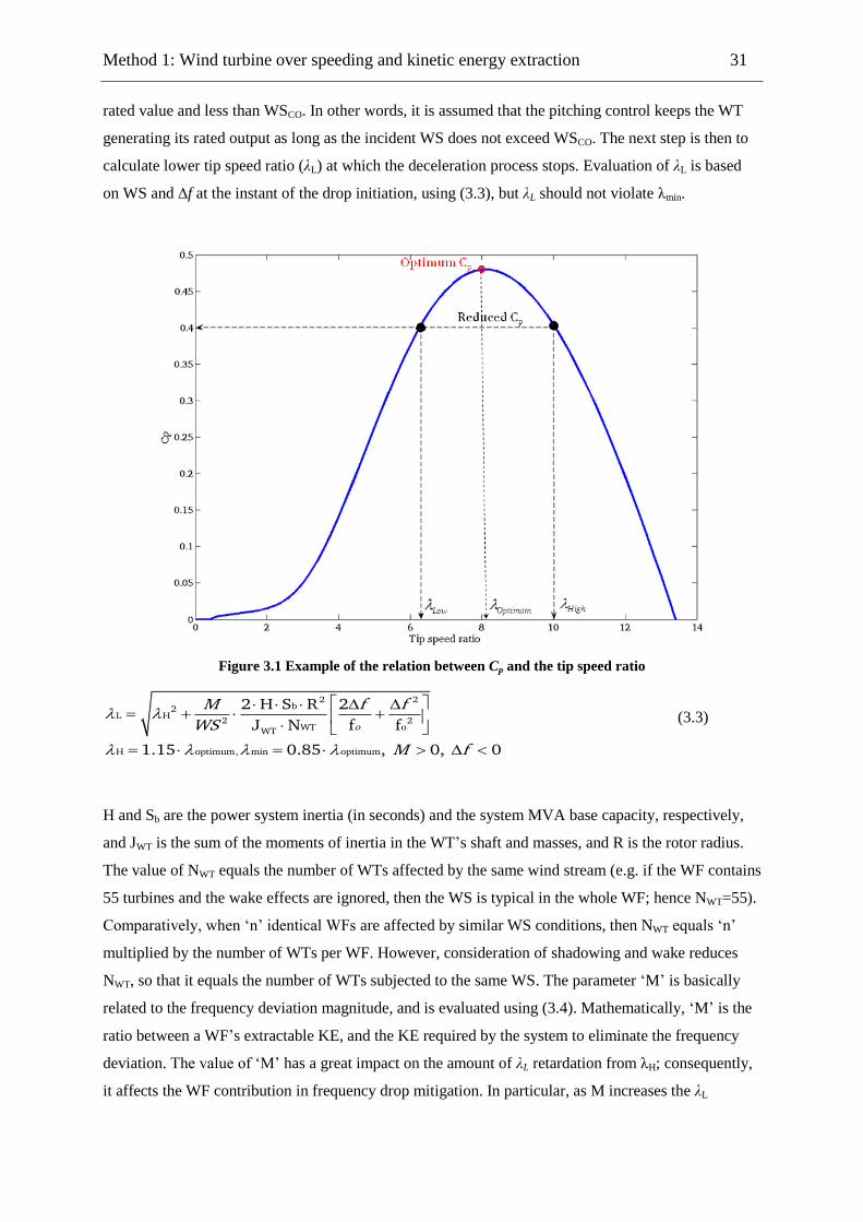
Method 1: Wind turbine over speeding and kinetic energy extraction 31
rated value and less than WSCO. In other words, it is assumed that the pitching control keeps the WT
generating its rated output as long as the incident WS does not exceed WSCO. The next step is then to
calculate lower tip speed ratio (λL) at which the deceleration process stops. Evaluation of λL is based
on WS and ∆f at the instant of the drop initiation, using (3.3), but λL should not violate λmin.
Figure 3.1 Example of the relation between Cp and the tip speed ratio
2 2b2
L H2 2
WT oWT
H optimum, min optimum
2 H S R 2
J N f f
1.15 0.85 , 0, 0
o
M f f
WS
M f
(3.3)
H and Sb are the power system inertia (in seconds) and the system MVA base capacity, respectively,
and JWT is the sum of the moments of inertia in the WT‘s shaft and masses, and R is the rotor radius.
The value of NWT equals the number of WTs affected by the same wind stream (e.g. if the WF contains
55 turbines and the wake effects are ignored, then the WS is typical in the whole WF; hence NWT=55).
Comparatively, when ‗n‘ identical WFs are affected by similar WS conditions, then NWT equals ‗n‘
multiplied by the number of WTs per WF. However, consideration of shadowing and wake reduces
NWT, so that it equals the number of WTs subjected to the same WS. The parameter ‗M‘ is basically
related to the frequency deviation magnitude, and is evaluated using (3.4). Mathematically, ‗M‘ is the
ratio between a WF‘s extractable KE, and the KE required by the system to eliminate the frequency
deviation. The value of ‗M‘ has a great impact on the amount of λL retardation from λH; consequently,
it affects the WF contribution in frequency drop mitigation. In particular, as M increases the λL

Method 1: Wind turbine over speeding and kinetic energy extraction 32
decreases (i.e., (2∆f /fo) >> (∆f 2/f
2o) and ∆f <0). Thus, further deceleration occurs and more KE is
extracted. However, the WS has also an impact on the retardation magnitude.
2 2min H WTWT2
22b
o o
J N 1, where 0
2 H S R 2
f f
M WS ff f
(3.4)
The ‗M‘ parameter may have a fixed or variable value according to the operator‘s policy. When ‗M‘ is
variable, its value is updated every simulation time step using (3.4) with respect to continuously
varying parameters, namely, WS and ∆f. A variable ‗M‘ mode tunes λL to higher values so that the WT
speed deterioration is alleviated and extracted KE is reduced. However, this operation mode shortens
recovery time (tR), thus the WT has better opportunity of supporting the system during further
consecutive drops, which might occur within a short time span just after the initial drop. However,
when the operator aims to utilize all the available stored KE to overcome certain frequency drop, ‗M‘
is adjusted to a constant value. According to (3.4), it is noticed that ‗M‘ is almost proportional to WS,
and inversely proportional to ∆f. Meanwhile, the other parameters are constants or pre-adjusted (e.g.,
λH). To utilize a portion from the extractable KE, ‗M‘ fixed value is reduced, thus estimated at deep ∆f
and low WS. This constant value is evaluated only once at certain pre-determined conditions, and is
then fixed throughout the whole simulation process. In addition, fixing ‗M‘ value at a low value
shortens tR; hence, WTs are able to provide support when the system suffers a second minor frequency
drop while it is recovering from the main one. In conclusion, the choice of using either a constant or a
variable selection for ‗M‘ involves potential risks that should be analysed thoroughly by the operator.
As an illustration of the use of tR, the WT should be partially unloaded for certain duration after the
support period ends so that it has the opportunity to return to its normal rotational speed (i.e. returning
to λH). In most literature tR is treated as a constant duration. In contrast however, this research
considers tR as a variable that is proportional to WS and λL, and which can be considered as a merit. In
particular, fixing tR wastes more energy as it keeps the WT partially loaded, even if it has already
recovered its default rotational speed. Therefore, estimating tR each time the WT supports the system
saves some energy and enables the WT to efficiently return to its normal operation. tR is calculated just
1 s before tS ends (i.e. at the end of the KE extraction interval) using (3.5). Whereas, CF is a certainty
factor greater than unity, and ensures that the rotational speed recovers to a normal value. The
evaluation of SlopeWT is made using (3.6), and is illustrated in Figure 3.2 according to the derived and
predetermined value of ts (15 s in this research work). Hence the corresponding slope (SlopeWT) is
evaluated at WSmin, so that a tough case is considered (SlopeWT=0.0147 rad/s2).
H L
F
WT
CR Slope
R
WSt (3.5)
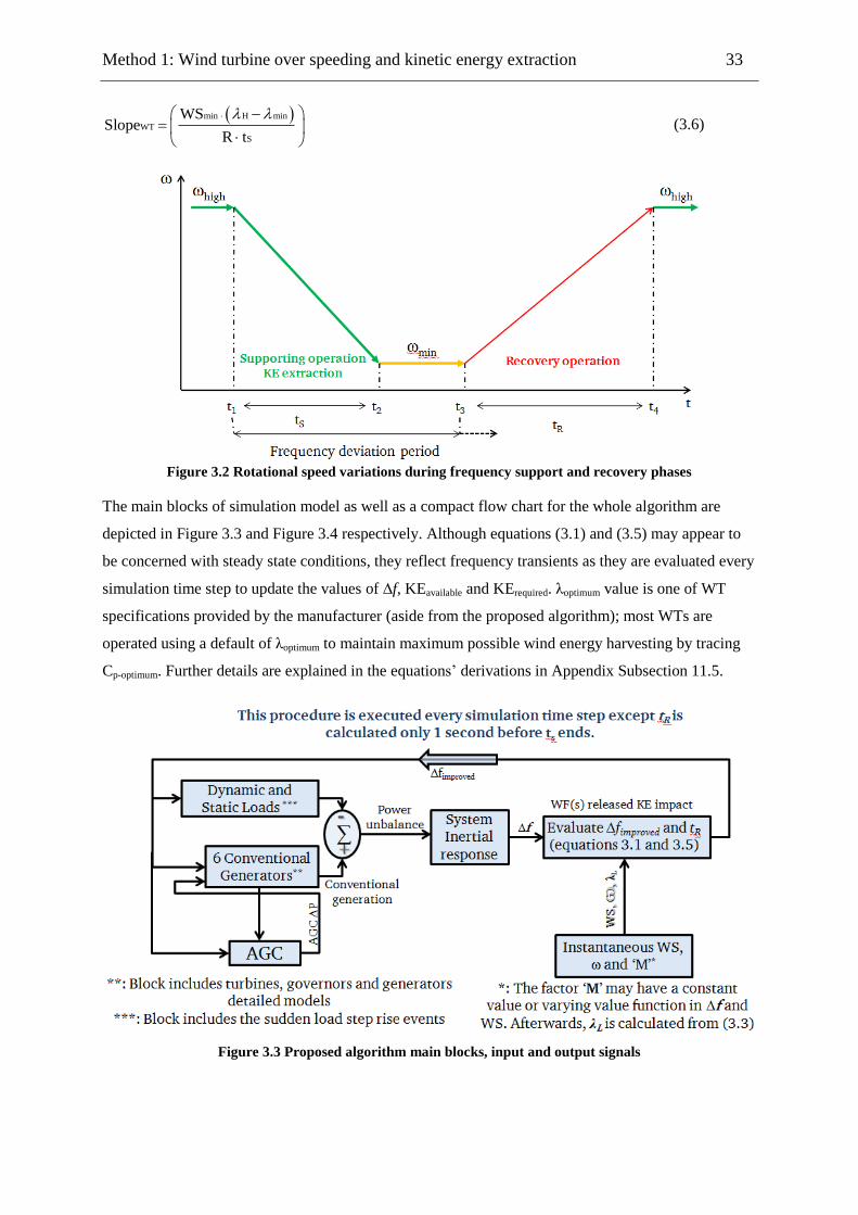
Method 1: Wind turbine over speeding and kinetic energy extraction 33
min H min
WT
S
WSSlope
R t
(3.6)
Figure 3.2 Rotational speed variations during frequency support and recovery phases
The main blocks of simulation model as well as a compact flow chart for the whole algorithm are
depicted in Figure 3.3 and Figure 3.4 respectively. Although equations (3.1) and (3.5) may appear to
be concerned with steady state conditions, they reflect frequency transients as they are evaluated every
simulation time step to update the values of ∆f, KEavailable and KErequired. λoptimum value is one of WT
specifications provided by the manufacturer (aside from the proposed algorithm); most WTs are
operated using a default of λoptimum to maintain maximum possible wind energy harvesting by tracing
Cp-optimum. Further details are explained in the equations‘ derivations in Appendix Subsection 11.5.
Figure 3.3 Proposed algorithm main blocks, input and output signals
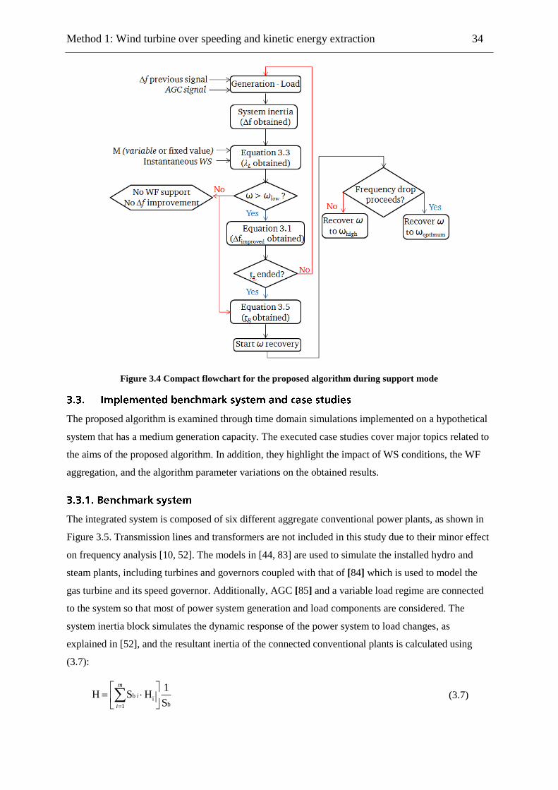
Method 1: Wind turbine over speeding and kinetic energy extraction 34
Figure 3.4 Compact flowchart for the proposed algorithm during support mode
The proposed algorithm is examined through time domain simulations implemented on a hypothetical
system that has a medium generation capacity. The executed case studies cover major topics related to
the aims of the proposed algorithm. In addition, they highlight the impact of WS conditions, the WF
aggregation, and the algorithm parameter variations on the obtained results.
The integrated system is composed of six different aggregate conventional power plants, as shown in
Figure 3.5. Transmission lines and transformers are not included in this study due to their minor effect
on frequency analysis [10, 52]. The models in [44, 83] are used to simulate the installed hydro and
steam plants, including turbines and governors coupled with that of [84] which is used to model the
gas turbine and its speed governor. Additionally, AGC [85] and a variable load regime are connected
to the system so that most of power system generation and load components are considered. The
system inertia block simulates the dynamic response of the power system to load changes, as
explained in [52], and the resultant inertia of the connected conventional plants is calculated using
(3.7):
b ib1
1H S H
S
m
i
i
(3.7)

Method 1: Wind turbine over speeding and kinetic energy extraction 35
Hi and Sbi are the inertia and rated MVA of power plant (i) respectively, and ‗m‘ is the number of
connected conventional plants. The integrated WSs array is based on the readings obtained at the
Za‘afrana WF, on the Red Sea shore in Egypt [86], where WS data are arranged chronologically in
one hour steps. Table 3.1 summarizes essential data in relation to the nature of WS at the chosen
location during winter. However, the frequency studies require high time resolution data, and hence,
the array steps of WSs need to be in the range of seconds. To overcome this problem, the algorithm
offered in [87] is implemented, so that as seen in one of the case studies the WS average value is
estimated every 25 s in addition to acknowledging wake and shadowing effects inside the WF.
Table 3.1 WindspeedstatisticsduringwinteratZa’afrana
Winter (08:00 to 21:00)
Value (m/s) Actual (every 2 h for 91 days) Generated array
Average 6.31 5.15
Max 11.09 15.65
Min 2.71 2.884
No. of events WS>=WSr 114/1183 (9.6%) 4290/46800 (9.2%)
No. of events WS<=WSCI 15/1183 (1.3%) 562/46800 (1.2%)
Figure 3.5 Implemented power system single line diagram
This research work has chosen to study system performance at a relatively variable WS, as this
emphasizes the influence of the proposed algorithm and the implemented system. The duration of the
simulation is 13 hours (08:00 to 21:00, which is equivalent to 46800s) throughout the winter season, as
WSs achieve the highest levels during this period. The integrated WT is GE-77, and it has (Ѡ vs.
PWTm) curves at several WSs, as previously presented in Figure 2.5. The moment of inertia (JWT) of
GE-77 is 543 kgm2.
The six case studies examine the wind energy integration impact on system frequency in different
circumstances during the specified hypothetical load step rise events mentioned, wherein the
magnitude of each step is stated as a percentage from Sb. The conditions examined include the
integration of WFs, with or without any changes in conventional generation capacity, coupled with
including or ignoring the wake effects. In addition, the proposed cases highlight the advantages and

Method 1: Wind turbine over speeding and kinetic energy extraction 36
disadvantages of fixing, or actively varying ‗M‘ during the KE extraction process. The influence of
delaying the AGC signal on the system frequency is also tested. A basic case study represents the
response of the benchmark system with no integrated WF, and it is therefore used as a reference to
compare and judge the results of other case studies. The default WF is composed of 55 GE-77 WTs.
When the wake effect is considered, the WF layout is divided into 5 rows, and each one is composed
of 11 WTs. The incident wind stream faces the WT blades directly in each row, if the stream
orientation angle is zero with respect to the WT horizontal axis [87]. In addition, the WS magnitude
changes from one row to another due to the shadowing effect from the towers and blades of the WTs
in the row in front. In contrast, when the wake effect is ignored, all WTs inside the WF are subjected
to identical WS. ‗M‘ is considered to be the variable in all case studies excluding cases four and six, as
explained in the following.
Case study 1: Single WF is integrated; wake effects and shadowing are ignored.
Case study 2: Single WF is integrated; wake effects and shadowing are acknowledged. For
simplicity, it is assumed that the WTs are arranged in regular rows and columns inside the WF. The
first row is subjected to the initial free stream of WS; afterwards the WS is reduced gradually in each
row in relation to the shadowing and wake effects of the towers. The average wake WS is evaluated at
each row using (3.8) depending on the WTs dimensions and other factors [87, 88, 89]. The thrust
coefficient (Ct) is evaluated using an empirical formula. WS(x) is the velocity in the wake at distance
x; and WSo is the free stream WS (i.e. the initial incident WS just before it hits the first WT and starts
to propagate through the WF). It is of note that the distance between successive WTs (x) is inversely
proportional to the reduction in WS(x). As an illustration, an increase in x achieves a useful curtailment
of the negative influence of the tower and shadowing on the WS magnitude projected on the next WT
blades. The second factor is R, as its increase amplifies the impact of the wake effects. In addition, the
time delay due to the propagation of the WS throughout the WF is included, as in (3.9) [63], where
Drow is the distance between two successive rows and is assumed to be 12·R while kw = 0.08. In
particular, tdelay interprets the time required by the wind stream to travel from one row to another, thus
WSo and WS(x) are asynchronous.
Table 3.2 Data of five step load increase events (percentage from Sb)
Value/Event Event 1 Event 2 Event 3 Event 4 Event 5
Load step, MW 97 (10.5%) 84 (9.1%) 110 (12%) 80 (8.7%) 108 (11.7%)
Start time, s 3078 12160 22180 33230 42280
Duration, s 2938 3220 3190 3040 2840
Method 1: Wind turbine over speeding and kinetic energy extraction 37
2
oo
2w o
3.5 m/s (2 WS 3.5 m/s)R( ) WS 1 1 1 C , C
k R WSt tWS x
x
( 3.8)
rowD( )
( )delayt x
WS x ( 3.9)
Case study 3: A gas plant is replaced by a certain number of WFs with an equivalent generation
capacity. It is well known that the annual average production of a WF is 20–30% of its nameplate
rating [89, 90]. This chapter assumes that the considered WF generates 20% of its aggregate power
rating (i.e. 55 · 1.5 MW · 20%=16.5 MW). However, the participation of the gas plant in load feeding
is 90 MW, therefore it needs to be replaced by 6 WFs (6·16.5=99 MW). In this case, the production of
the WFs (namely 99 MW), reflects 11% wind energy penetration of the total scheduled generated
power. This penetration level is subjected to minor and major fluctuations according to the
instantaneous WS (e.g. wind energy penetration reaches 38% when the combined WFs generate 70%
of their aggregate rated output). This replacement procedure affects normal operation, in addition to
system frequency response during frequency drops due to the continuous WS variations. Therefore,
this chapter focuses on the WF contribution during frequency drop events. Note that the six WFs are
aggregated as one WT facing the same WS, because it is assumed that the WS is similar in the six
WFs. This case study also ignores the wake and shadowing effects.
Case study 4: This has similar conditions to Case study 3, and the only difference is that this study
keeps ‗M‘ as a constant value, which is calculated at 56% from the WF frequency deviation limit,
namely, 1% from the nominal frequency (i.e. ∆f = 50 -0.01 0.56 =-0.28 Hz). This ∆f value is
selected because it is assumed that WFs do not contribute to frequency recovery if ∆f exceeds this
limit, but they operate normally to avoid loss of synchronization. In other words, the ‗M‘ value
evaluated at ∆f = -0.28 Hz and at a moderate WS equals the average between WSr and WSmin, namely,
6.5 m/s. Consequently, ‗M‘ equals 4.4397 using (11.10) as illustrated in Appendix 11.5.
Case studies 5 and 6: Case study 5 has similar conditions to Case study 3, and Case study 6 is
similar to Case study 4, except for the use of intended delay in the AGC signal in Case studies 5 and 6.
The AGC signal is delayed by 40 s to emphasise the impact of the offered technique, to ensure that it
does not merge with the reactions of the conventional generator.
The next two sub-sections summarize the basic comments and discussion obtained from the results,
figures, and tables. The first subsection focuses on the system frequency response of all case studies,
and the second subsection discusses variations in the parameters of the proposed algorithm.
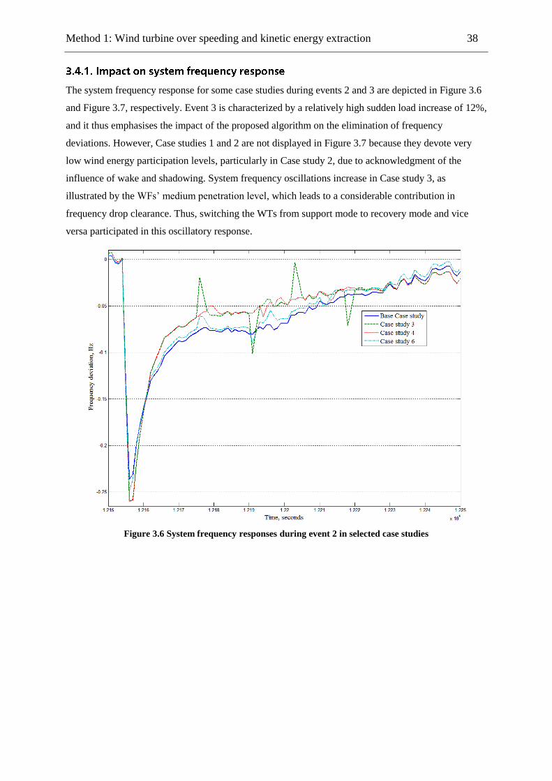
Method 1: Wind turbine over speeding and kinetic energy extraction 38
The system frequency response for some case studies during events 2 and 3 are depicted in Figure 3.6
and Figure 3.7, respectively. Event 3 is characterized by a relatively high sudden load increase of 12%,
and it thus emphasises the impact of the proposed algorithm on the elimination of frequency
deviations. However, Case studies 1 and 2 are not displayed in Figure 3.7 because they devote very
low wind energy participation levels, particularly in Case study 2, due to acknowledgment of the
influence of wake and shadowing. System frequency oscillations increase in Case study 3, as
illustrated by the WFs‘ medium penetration level, which leads to a considerable contribution in
frequency drop clearance. Thus, switching the WTs from support mode to recovery mode and vice
versa participated in this oscillatory response.
Figure 3.6 System frequency responses during event 2 in selected case studies
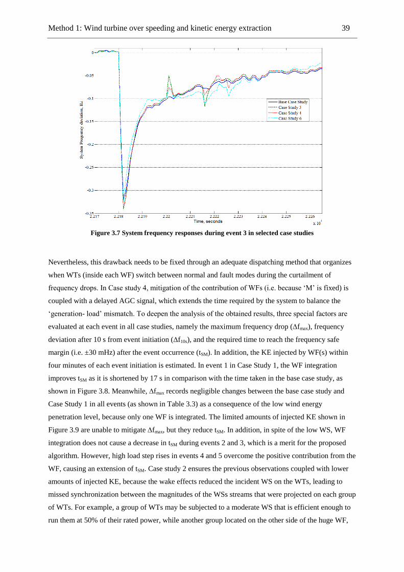
Method 1: Wind turbine over speeding and kinetic energy extraction 39
Figure 3.7 System frequency responses during event 3 in selected case studies
Nevertheless, this drawback needs to be fixed through an adequate dispatching method that organizes
when WTs (inside each WF) switch between normal and fault modes during the curtailment of
frequency drops. In Case study 4, mitigation of the contribution of WFs (i.e. because ‗M‘ is fixed) is
coupled with a delayed AGC signal, which extends the time required by the system to balance the
‗generation- load‘ mismatch. To deepen the analysis of the obtained results, three special factors are
evaluated at each event in all case studies, namely the maximum frequency drop (∆fmax), frequency
deviation after 10 s from event initiation (∆f10s), and the required time to reach the frequency safe
margin (i.e. ±30 mHz) after the event occurrence (tSM). In addition, the KE injected by WF(s) within
four minutes of each event initiation is estimated. In event 1 in Case Study 1, the WF integration
improves tSM as it is shortened by 17 s in comparison with the time taken in the base case study, as
shown in Figure 3.8. Meanwhile, ∆fmax records negligible changes between the base case study and
Case Study 1 in all events (as shown in Table 3.3) as a consequence of the low wind energy
penetration level, because only one WF is integrated. The limited amounts of injected KE shown in
Figure 3.9 are unable to mitigate ∆fmax, but they reduce tSM. In addition, in spite of the low WS, WF
integration does not cause a decrease in tSM during events 2 and 3, which is a merit for the proposed
algorithm. However, high load step rises in events 4 and 5 overcome the positive contribution from the
WF, causing an extension of tSM. Case study 2 ensures the previous observations coupled with lower
amounts of injected KE, because the wake effects reduced the incident WS on the WTs, leading to
missed synchronization between the magnitudes of the WSs streams that were projected on each group
of WTs. For example, a group of WTs may be subjected to a moderate WS that is efficient enough to
run them at 50% of their rated power, while another group located on the other side of the huge WF,
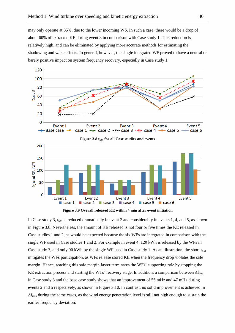
Method 1: Wind turbine over speeding and kinetic energy extraction 40
may only operate at 35%, due to the lower incoming WS. In such a case, there would be a drop of
about 60% of extracted KE during event 3 in comparison with Case study 1. This reduction is
relatively high, and can be eliminated by applying more accurate methods for estimating the
shadowing and wake effects. In general, however, the single integrated WF proved to have a neutral or
barely positive impact on system frequency recovery, especially in Case study 1.
Figure 3.8 tSM for all Case studies and events
Figure 3.9 Overall released KE within 4 min after event initiation
In Case study 3, tSM is reduced dramatically in event 2 and considerably in events 1, 4, and 5, as shown
in Figure 3.8. Nevertheless, the amount of KE released is not four or five times the KE released in
Case studies 1 and 2, as would be expected because the six WFs are integrated in comparison with the
single WF used in Case studies 1 and 2. For example in event 4, 120 kWh is released by the WFs in
Case study 3, and only 90 kWh by the single WF used in Case study 1. As an illustration, the short tSM
mitigates the WFs participation, as WFs release stored KE when the frequency drop violates the safe
margin. Hence, reaching this safe margin faster terminates the WFs‘ supporting role by stopping the
KE extraction process and starting the WTs‘ recovery stage. In addition, a comparison between ∆f10s
in Case study 3 and the base case study shows that an improvement of 55 mHz and 47 mHz during
events 2 and 5 respectively, as shown in Figure 3.10. In contrast, no solid improvement is achieved in
∆fmax during the same cases, as the wind energy penetration level is still not high enough to sustain the
earlier frequency deviation.
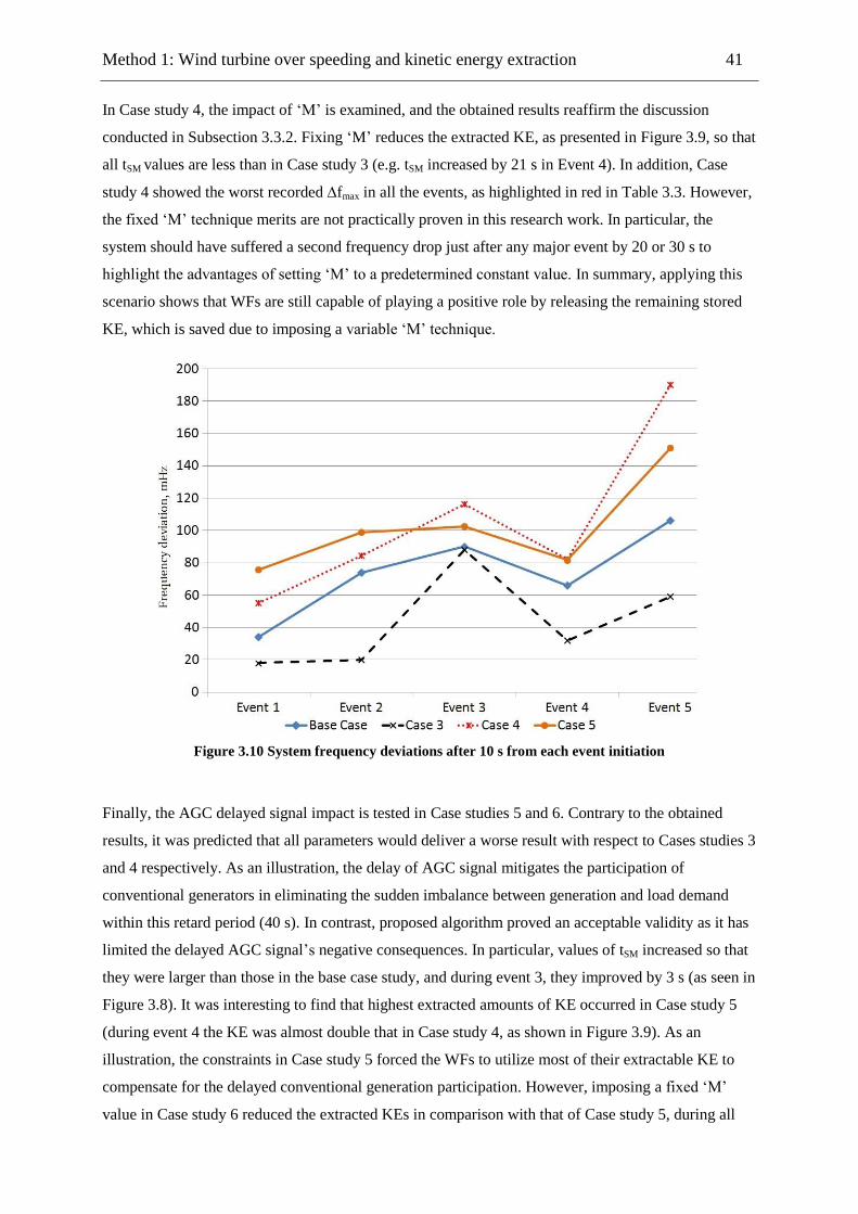
Method 1: Wind turbine over speeding and kinetic energy extraction 41
In Case study 4, the impact of ‗M‘ is examined, and the obtained results reaffirm the discussion
conducted in Subsection 3.3.2. Fixing ‗M‘ reduces the extracted KE, as presented in Figure 3.9, so that
all tSM values are less than in Case study 3 (e.g. tSM increased by 21 s in Event 4). In addition, Case
study 4 showed the worst recorded ∆fmax in all the events, as highlighted in red in Table 3.3. However,
the fixed ‗M‘ technique merits are not practically proven in this research work. In particular, the
system should have suffered a second frequency drop just after any major event by 20 or 30 s to
highlight the advantages of setting ‗M‘ to a predetermined constant value. In summary, applying this
scenario shows that WFs are still capable of playing a positive role by releasing the remaining stored
KE, which is saved due to imposing a variable ‗M‘ technique.
Figure 3.10 System frequency deviations after 10 s from each event initiation
Finally, the AGC delayed signal impact is tested in Case studies 5 and 6. Contrary to the obtained
results, it was predicted that all parameters would deliver a worse result with respect to Cases studies 3
and 4 respectively. As an illustration, the delay of AGC signal mitigates the participation of
conventional generators in eliminating the sudden imbalance between generation and load demand
within this retard period (40 s). In contrast, proposed algorithm proved an acceptable validity as it has
limited the delayed AGC signal‘s negative consequences. In particular, values of tSM increased so that
they were larger than those in the base case study, and during event 3, they improved by 3 s (as seen in
Figure 3.8). It was interesting to find that highest extracted amounts of KE occurred in Case study 5
(during event 4 the KE was almost double that in Case study 4, as shown in Figure 3.9). As an
illustration, the constraints in Case study 5 forced the WFs to utilize most of their extractable KE to
compensate for the delayed conventional generation participation. However, imposing a fixed ‗M‘
value in Case study 6 reduced the extracted KEs in comparison with that of Case study 5, during all

Method 1: Wind turbine over speeding and kinetic energy extraction 42
events. In addition, delaying the AGC signal exacerbated ∆f10s in Case study 5, compared to results in
Case study 3, during all events. For example, ∆f10s decreased by 61 mHz and by 45 mHz in events 1
and 4 respectively, as shown in Figure 3.10, and the worst results occurred in event 5 (130 mHz) due
to the highest load rise event. It is considered that the low wind energy penetration level (i.e., 11%),
coupled with the low incident WS during some events cause this negative influence. It is illustrative to
mention that ∆fmax is almost similar in Case studies 5 and 6 throughout the five events, as shown in
Table 3.3. This ensures that the evaluation method of ‗M‘, using either a variable or pre-determined
fixed value, has a neutral impact on the system response within such an early stage just after the
occurrence of the frequency excursion.
Table 3.3 Max. Frequency drops in all cases (worst deviation at each event marked in red)
Case/Index Max frequency drop, mHz
Event1 Event2 Event3 Event4 Event5
Basic 254.07 248.39 320.5 225.43 354.43
1 253.06 248.49 320.58 225.02 354.06
2 253.06 248.49 320.58 225.02 354.06
3 247.58 259.89 340.07 230.19 373.86
4 246.49 259.95 340.08 230.98 361.39
5 245.43 249.01 329.54 198.35 320.87
6 243.12 248.89 329.34 193.08 322.28
This subsection draws attention to the variations in the main parameters of the proposed algorithm,
namely: WS, λL, and tR, in addition to the expected improvement in ∆f. It is of note that the displayed
frequency values in the following figures represent the improvement magnitude and not the new
deviation. For example, when ∆f actual value is -0.6 Hz and the expected frequency improvement
depicted in a figure is 0.06 Hz, this means that ∆fimproved is -0.54 Hz. Initially, it is important to explain
why the frequency deviation improvements in Figure 3.11 and Figure 3.12 are constant, even though
the WS and actual frequency deviation are continuously changing. Generally, the fixed frequency
deviation improvement is related to the role played by the variable ‗M‘ value, as it keeps the expected
∆f enhancement constant independent from other factors. Consequently, power system operators are
aware that the expected system performance and the integration of WF(s) will not lead to extremely
unpredictable changes in frequency response. It is of note that the time delay of the electronic power
devices is ignored, hence WF support starts just after the frequency drop occurs, as shown in Figure
3.11 (i.e., event 5 starts at 4.228·104 s). Before the KE extraction process starts, tR and λL oscillate
continuously, based on the instantaneous WS (as depicted in Figure 3.11(b) and (c) respectively). As
soon as ∆f violates the safety margin, the proposed algorithm records the λL value at the beginning of
each tS and keeps it fixed. In spite of integrating only one WF in relation to the moderate WS in Case
study 1 event 5, the expected ∆f enhancement was encouraging (6.5 mHz). Meanwhile the value of tR
was not very long (15 - 22 s), and thus it is considered that the WF could re-support the system if a
second successive drop occurred a short time after the first one.
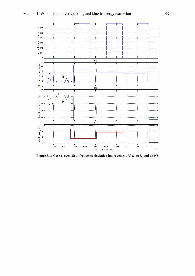
Method 1: Wind turbine over speeding and kinetic energy extraction 43
Figure 3.11 Case 1, event 5: a) frequency deviation improvement, b) tR, c) λL, and d) WS
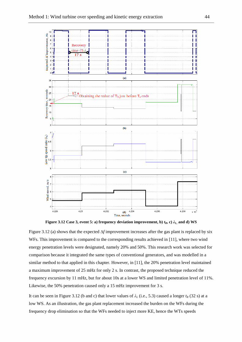
Method 1: Wind turbine over speeding and kinetic energy extraction 44
Figure 3.12 Case 3, event 5: a) frequency deviation improvement, b) tR, c) λL, and d) WS
Figure 3.12 (a) shows that the expected ∆f improvement increases after the gas plant is replaced by six
WFs. This improvement is compared to the corresponding results achieved in [11], where two wind
energy penetration levels were designated, namely 20% and 50%. This research work was selected for
comparison because it integrated the same types of conventional generators, and was modelled in a
similar method to that applied in this chapter. However, in [11], the 20% penetration level maintained
a maximum improvement of 25 mHz for only 2 s. In contrast, the proposed technique reduced the
frequency excursion by 11 mHz, but for about 10s at a lower WS and limited penetration level of 11%.
Likewise, the 50% penetration caused only a 15 mHz improvement for 3 s.
It can be seen in Figure 3.12 (b and c) that lower values of λL (i.e., 5.3) caused a longer tR (32 s) at a
low WS. As an illustration, the gas plant replacement increased the burden on the WFs during the
frequency drop elimination so that the WFs needed to inject more KE, hence the WTs speeds
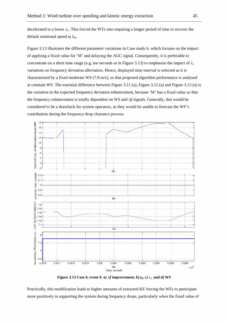
Method 1: Wind turbine over speeding and kinetic energy extraction 45
decelerated to a lower λL. This forced the WTs into requiring a longer period of time to recover the
default rotational speed at λH.
Figure 3.13 illustrates the different parameter variations in Case study 6, which focuses on the impact
of applying a fixed value for ‗M‘ and delaying the AGC signal. Consequently, it is preferable to
concentrate on a short time range (e.g. ten seconds as in Figure 3.13) to emphasise the impact of λL
variations on frequency deviation alleviation. Hence, displayed time interval is selected as it is
characterized by a fixed moderate WS (7.8 m/s), so that proposed algorithm performance is analysed
at constant WS. The essential difference between Figure 3.11 (a), Figure 3.12 (a) and Figure 3.13 (a) is
the variation in the expected frequency deviation enhancement, because ‗M‘ has a fixed value so that
the frequency enhancement is totally dependent on WS and ∆f signals. Generally, this would be
considered to be a drawback for system operators, as they would be unable to forecast the WF‘s
contribution during the frequency drop clearance process.
Figure 3.13 Case 6, event 4: a) ∆f improvement, b) tR, c) λL, and d) WS
Practically, this modification leads to higher amounts of extracted KE forcing the WFs to participate
more positively in supporting the system during frequency drops, particularly when the fixed value of

Method 1: Wind turbine over speeding and kinetic energy extraction 46
‗M‘ is reduced. Conversely, increasing the fixed value of ‗M‘ saves a portion of the stored KE; hence,
the WF(s) would be able to support the system if it suffered a second successive frequency drop after
the major one within a very short time span. Moreover, the intended delay in the AGC signal could be
an option for system operators if a system frequency drop incident overlaps with moderate or high
WSs (i.e., relatively high WFs production), thereby attaining solid improvements in frequency
excursion elimination and reducing stress on conventional units.
This chapter proposed an algorithm to control the extraction of KE during power system frequency
drops, in addition to quantifying this KE and estimating the expected system frequency deviation
curtailment. The offered algorithm integration with variable speed WTs proved to be feasible and
practical, because it depends on special settings for the WT rotational speed. Moreover, some
measurements signals are required as inputs, namely the instantaneous approximate WS and the
system frequency deviation. The algorithm flexibility (i.e., it can be applied to any type of variable
speed WT), coupled with its independency from pitch angle, are two acknowledged merits. The
offered algorithm has been tested on a relatively medium capacity hypothetical system that includes
the most dominant conventional generation types, in addition to detailed models of turbines and
governors. More than 10% of the system generation capacity is replaced by wind energy in the four
case studies. Results enable an insight into the feasibility of the offered algorithm, and reflect the
achieved improvements in frequency response. In particular, wind energy integration has a positive
impact on the system‘s response in most of the case studies, and in rare cases, it had a neutral or
negative influence on some factors. The selection between constant or variable ‗M‘ is a trade-off
between reducing lost energy or triggering the optimum possible support (constant mode) on one side,
and gaining a higher certainty in predicting system performance during frequency drops (variable
mode) on the other side.

Method 2: Wind turbine de-loading/overloading 47
The proposed algorithm has two operational modes, normal and support, which causes the WT to
provide extra active power during frequency drops. The normal mode controls WT output through
rotational speed and pitch angle adjustments according to the instantaneous WS category. Algorithm
parameters are tuned based on WT specifications and average WS conditions in the WF location. The
novel algorithm of normal operation ensures the positive contribution of WTs in the curtailment of
frequency deviations, regardless of the instantaneous WS conditions. The innovative concept of
merging pitch and rotational speed de-loading with overproduction deceleration is implemented to
avoid continuous de-loading; hence, there is a reduction in the wind energy wasted. The WT generator
is overloaded when a frequency deviation is accompanied by high WSs, and the amount of extra wind
energy produced during frequency deviation clearance is then estimated at different WS conditions,
including sever WS drops. An islanded medium capacity hypothetical system is then implemented to
examine the proposed algorithm.
WT operation is related to the rotational speed and pitch angle, with WS as the factor that is unable to
be controlled. Controlled parameters are used in different operational regions so that the WT is always
ready to contribute positively in the elimination of frequency drops. The operational regions are
defined using certain WS categories with pivot values decided based on the WT type and the WS
nature at the WF location. The WS categories are initially defined, and the normal and support
operational modes in each operational region are then explained and illustrated using suitable figures
and examples. The GE-77 embedded model in Simulink is applied, and it receives three inputs; WS,
pitch angle, and rotational speed.
WS values that determine the operational regions of the proposed algorithm are defined according to
the next procedure.
Firstly, the two main parameters are estimated, namely base wind speed (WSB), and base mechanical
rotational of rotor (Ѡbase):
Base Rotational Speed (Ѡbase)
This value is selected according to the WS nature in the WT location and is adjusted so that the WT
produces the optimum allowed mechanical output power at the dominant WS conditions, namely the
annual average WS in the concerned WF location (WSavg). Note that values of Ѡbase are less than the
2Major content of this chapter is published in IET journal of Generation, Transmission and Distribution as indicated in
Related publications list

Method 2: Wind turbine de-loading/overloading 48
maximum allowed Ѡ according to WT specifications. In fact, the range of Ѡ (in r/s) depends on the
WT type and the installed converter specifications, as explained earlier in Subsection 2.2. In this
chapter, WSavg is 8 m/s and GE-77 has Ѡ range from 1.15 rad/s to 2.51 rad/s [17]. Thus, maximum
PWTm at this WS is 0.47 pu, at Ѡbase=1.66 rad/s=1 pu. Thus, Ѡmax = 1.51 pu and Ѡmin = 0.69 pu.
Base WS (WSB)
WSB is the WS at which Ѡ equals 1 pu and generating base power (PWTm = PB), which is less than 1
pu. PB is assumed to be in the range of 0.65 to 0.75 pu at Ѡ = Ѡbase.
Cut in WS (WSCI)
Below this value WS is too slow to run the WT, and therefore PWTm = 0.
Low WS (WSlow)
At this WS and Ѡbase, PWTm is in the range of 0.2 to 0.25 pu.
High WS (WShigh)
At this WS, PWTm ≈ 1 pu at Ѡbase and a zero pitch angle. Note that, WShigh is not necessarily the WSR
mentioned by the WT manufacturer, as it depends on the suggested Ѡbase.
It is of note that based on comprehensive trials at different values for WSB, it was found that WSlow ≈
0.7· WSB and WShigh ≈ 1.16·WSB. Numerical values for the imposed WS classes in this research work
are presented in Table 4.1.
The offered algorithm is only applicable to WTs equipped with converters that allow rotor rotational
speed variations and keep the grid connection at a fixed synchronized speed. It is therefore suitable for
DFIG type 3, and full rated converter type 4 (e.g. Enercon 101).
Table 4.1 Major WS categories values in m/s
WSavg WSCI WSlow WSB WShigh WSCO
8 3.5 6.5 9.5 (PB = 0.7 pu) 11 25
This subsection explains the four operational regions that drive the WT according to WS classes, and
each region has two modes (Normal and Support). The proposed algorithm makes a compromise
between three methods to provide instant support during frequency events, namely pitch de-loading,
decelerating overproduction, and temporary overloading. The levels of support in the first and second
regions differ according to the WS conditions and WT specifications. Meanwhile, the overloading
mode provides a fixed amount of power surge as long as the WS is above the predetermined threshold.
Pitch de-loading is illustrated by WT output reduction in relation to increasing the pitch angle. For
instance, at a certain WS, WT output is ‗X‘ at a zero pitch angle [91]. When de-loading is activated,
the output power is adjusted to ‗X· (1-DF)‘, where DF is the de-loading factor. Thus, the pitch angle is

Method 2: Wind turbine de-loading/overloading 49
adjusted through a closed loop controller, so that the WT output satisfies the de-loaded reference. In
short, the de-loaded output is less than the ‗zero-pitch‘ output (i.e., optimum power) by DF%.
In addition, overproduction refers to forcing the WT to produce power exceeding the available PWTm.
The source of this extra power is the extraction of stored KE in the WT rotating parts. Therefore,
overproduction leads to WT deceleration (i.e., Ѡ decreases) and it must be stopped at certain critical
Ѡmin to avoid loss of synchronism [80], or at a slightly higher value as explained later.
Region 1: WS < WSCI or WS > WSCO
The WT stops due to very low WS or to protect WT from excess mechanical stresses at very high
WSs, consequently PWTm = 0 in both cases.
Region 2: WSCI<WS< WSlow
Normal mode
Pitch de-loading is deactivated (β = 0), Ѡ =1 pu and PWTm is evaluated using (2.1).
Support mode
Overproduction mode is initiated by adjusting the WT output reference to ‗(1+2·DF) ·value of PWTm at
the initiation instant of support mode‘ at Ѡ=1 pu. Using the DF value in setting the overproduced
power makes the size of the step increase in output power comparable to the corresponding rise in the
case of de-loading mode commencement. It is of note that, no de-loading occurs in this category, and
only the numerical value of DF is considered. Overproduction continues until the frequency drop is
cleared or until Ѡ sinks to Ѡmin. Any deterioration of Ѡ, and estimation of its instantaneous value, is
described using (4.1). In brief, Ѡ is fixed to 1 pu at normal operation and then starts decelerating just
after the frequency drop occurs, which is accompanied by the steep rise in output power, as shown in
Figure 4.1. After this, Ѡ builds up again and returns to 1 pu after the WT is switched to normal mode.
However, during the recovery process the WT output is reduced by 10% from the available PWTm, so
that the WT is able to accelerate to a Ѡbase as shown in Figure 4.1.
WT
F
1,
J
(1 2 D )
em e e
e m normal
d PWTTWT TWT TWT
dt
PWT PWT
(4.1)
TWTm and TWTe are the mechanical and electrical torques respectively.
Region 3: WSlow<WS< WShigh
Normal mode
The output power is de-loaded by DF calculated based on the required extra active power (∆PWT) from
the WT during a frequency drop. Hence, it is preferred to calculate ∆PWT at WSavg to avoid worst-case
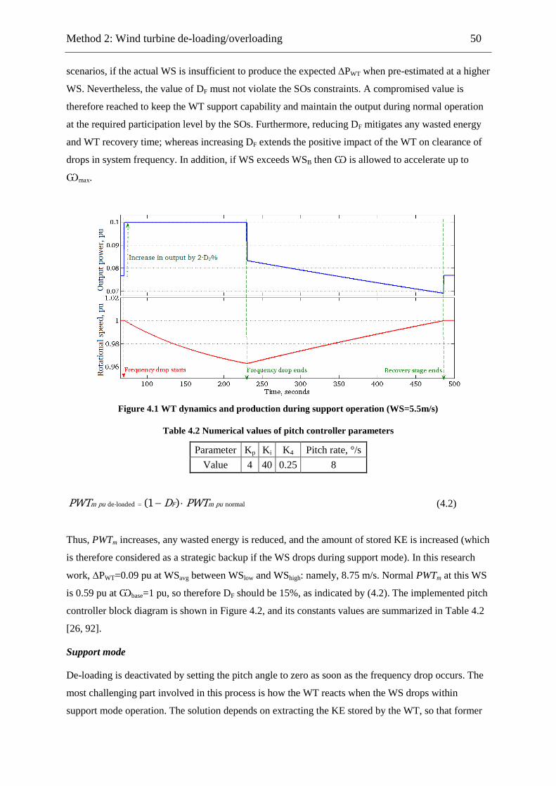
Method 2: Wind turbine de-loading/overloading 50
scenarios, if the actual WS is insufficient to produce the expected ∆PWT when pre-estimated at a higher
WS. Nevertheless, the value of DF must not violate the SOs constraints. A compromised value is
therefore reached to keep the WT support capability and maintain the output during normal operation
at the required participation level by the SOs. Furthermore, reducing DF mitigates any wasted energy
and WT recovery time; whereas increasing DF extends the positive impact of the WT on clearance of
drops in system frequency. In addition, if WS exceeds WSB then Ѡ is allowed to accelerate up to
Ѡmax.
Figure 4.1 WT dynamics and production during support operation (WS=5.5m/s)
Table 4.2 Numerical values of pitch controller parameters
Parameter Kp Ki K4 Pitch rate, °/s
Value 4 40 0.25 8
de-loaded normal (1 )m pu F m puPWT D PWT (4.2)
Thus, PWTm increases, any wasted energy is reduced, and the amount of stored KE is increased (which
is therefore considered as a strategic backup if the WS drops during support mode). In this research
work, ∆PWT=0.09 pu at WSavg between WSlow and WShigh: namely, 8.75 m/s. Normal PWTm at this WS
is 0.59 pu at Ѡbase=1 pu, so therefore DF should be 15%, as indicated by (4.2). The implemented pitch
controller block diagram is shown in Figure 4.2, and its constants values are summarized in Table 4.2
[26, 92].
Support mode
De-loading is deactivated by setting the pitch angle to zero as soon as the frequency drop occurs. The
most challenging part involved in this process is how the WT reacts when the WS drops within
support mode operation. The solution depends on extracting the KE stored by the WT, so that former
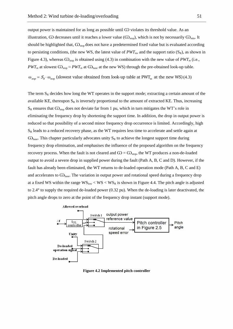
Method 2: Wind turbine de-loading/overloading 51
output power is maintained for as long as possible until Ѡ violates its threshold value. As an
illustration, Ѡ decreases until it reaches a lower value (Ѡstop), which is not by necessarily Ѡmin. It
should be highlighted that, Ѡstop does not have a predetermined fixed value but is evaluated according
to persisting conditions, (the new WS, the latest value of PWTm, and the support ratio (SR), as shown in
Figure 4.3), whereas Ѡstop is obtained using (4.3) in combination with the new value of PWTm (i.e.,
PWTm at slowest Ѡstop ≈ PWTm at Ѡbase at the new WS) through the pre-obtained look-up table.
ω ωstop m(slowest value obtained from look-up table at PWT at the new WS)stop RS (4.3)
The term SR decides how long the WT operates in the support mode; extracting a certain amount of the
available KE, thereupon SR is inversely proportional to the amount of extracted KE. Thus, increasing
SR ensures that Ѡstop does not deviate far from 1 pu, which in turn mitigates the WT‘s role in
eliminating the frequency drop by shortening the support time. In addition, the drop in output power is
reduced so that possibility of a second minor frequency drop occurrence is limited. Accordingly, high
SR leads to a reduced recovery phase, as the WT requires less time to accelerate and settle again at
Ѡbase. This chapter particularly advocates unity SR to achieve the longest support time during
frequency drop elimination, and emphasises the influence of the proposed algorithm on the frequency
recovery process. When the fault is not cleared and Ѡ = Ѡstop, the WT produces a non-de-loaded
output to avoid a severe drop in supplied power during the fault (Path A, B, C and D). However, if the
fault has already been eliminated, the WT returns to de-loaded operation mode (Path A, B, C and E)
and accelerates to Ѡbase. The variation in output power and rotational speed during a frequency drop
at a fixed WS within the range WSlow < WS < WSR is shown in Figure 4.4. The pitch angle is adjusted
to 2.4° to supply the required de-loaded power (0.32 pu). When the de-loading is later deactivated, the
pitch angle drops to zero at the point of the frequency drop instant (support mode).
Figure 4.2 Implemented pitch controller
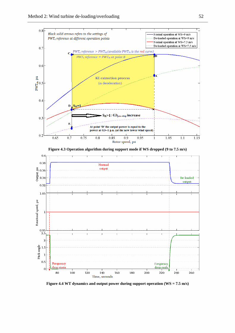
Method 2: Wind turbine de-loading/overloading 52
Figure 4.3 Operation algorithm during support mode if WS dropped (9 to 7.5 m/s)
Figure 4.4 WT dynamics and output power during support operation (WS = 7.5 m/s)
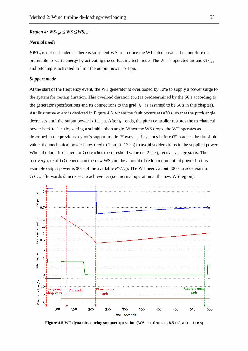
Method 2: Wind turbine de-loading/overloading 53
Region 4: WShigh ≤ WS ≤ WSCO
Normal mode
PWTm is not de-loaded as there is sufficient WS to produce the WT rated power. It is therefore not
preferable to waste energy by activating the de-loading technique. The WT is operated around Ѡmax
and pitching is activated to limit the output power to 1 pu.
Support mode
At the start of the frequency event, the WT generator is overloaded by 10% to supply a power surge to
the system for certain duration. This overload duration (tOL) is predetermined by the SOs according to
the generator specifications and its connections to the grid (tOL is assumed to be 60 s in this chapter).
An illustrative event is depicted in Figure 4.5, where the fault occurs at t=70 s, so that the pitch angle
decreases until the output power is 1.1 pu. After tOL ends, the pitch controller restores the mechanical
power back to 1 pu by setting a suitable pitch angle. When the WS drops, the WT operates as
described in the previous region‘s support mode. However, if tOL ends before Ѡ reaches the threshold
value, the mechanical power is restored to 1 pu. (t=130 s) to avoid sudden drops in the supplied power.
When the fault is cleared, or Ѡ reaches the threshold value (t= 214 s), recovery stage starts. The
recovery rate of Ѡ depends on the new WS and the amount of reduction in output power (in this
example output power is 90% of the available PWTm). The WT needs about 300 s to accelerate to
Ѡbase, afterwards β increases to achieve DF (i.e., normal operation at the new WS region).
Figure 4.5 WT dynamics during support operation (WS =11 drops to 8.5 m/s at t = 110 s)
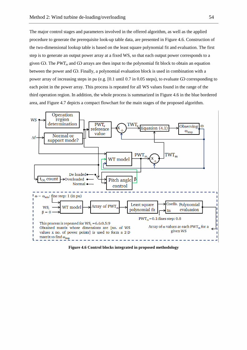
Method 2: Wind turbine de-loading/overloading 54
The major control stages and parameters involved in the offered algorithm, as well as the applied
procedure to generate the prerequisite look-up table data, are presented in Figure 4.6. Construction of
the two-dimensional lookup table is based on the least square polynomial fit and evaluation. The first
step is to generate an output power array at a fixed WS, so that each output power corresponds to a
given Ѡ. The PWTm and Ѡ arrays are then input to the polynomial fit block to obtain an equation
between the power and Ѡ. Finally, a polynomial evaluation block is used in combination with a
power array of increasing steps in pu (e.g. [0.1 until 0.7 in 0.05 steps), to evaluate Ѡ corresponding to
each point in the power array. This process is repeated for all WS values found in the range of the
third operation region. In addition, the whole process is summarized in Figure 4.6 in the blue bordered
area, and Figure 4.7 depicts a compact flowchart for the main stages of the proposed algorithm.
Figure 4.6 Control blocks integrated in proposed methodology
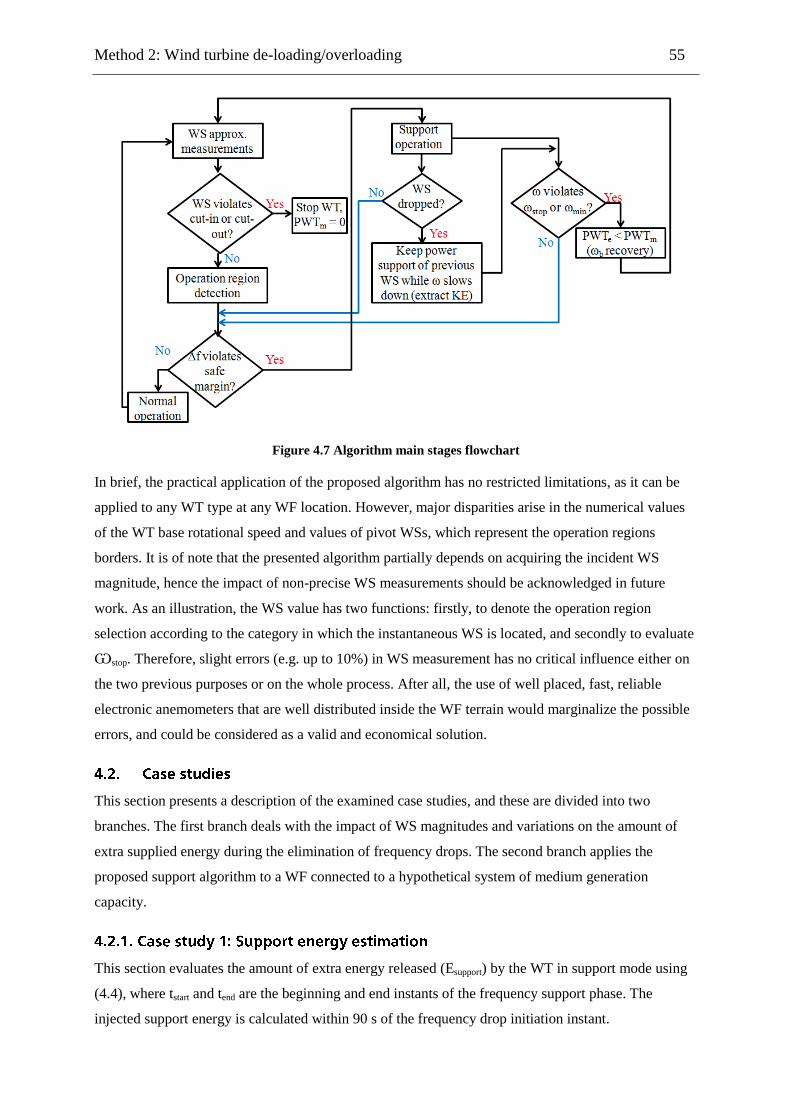
Method 2: Wind turbine de-loading/overloading 55
Figure 4.7 Algorithm main stages flowchart
In brief, the practical application of the proposed algorithm has no restricted limitations, as it can be
applied to any WT type at any WF location. However, major disparities arise in the numerical values
of the WT base rotational speed and values of pivot WSs, which represent the operation regions
borders. It is of note that the presented algorithm partially depends on acquiring the incident WS
magnitude, hence the impact of non-precise WS measurements should be acknowledged in future
work. As an illustration, the WS value has two functions: firstly, to denote the operation region
selection according to the category in which the instantaneous WS is located, and secondly to evaluate
Ѡstop. Therefore, slight errors (e.g. up to 10%) in WS measurement has no critical influence either on
the two previous purposes or on the whole process. After all, the use of well placed, fast, reliable
electronic anemometers that are well distributed inside the WF terrain would marginalize the possible
errors, and could be considered as a valid and economical solution.
This section presents a description of the examined case studies, and these are divided into two
branches. The first branch deals with the impact of WS magnitudes and variations on the amount of
extra supplied energy during the elimination of frequency drops. The second branch applies the
proposed support algorithm to a WF connected to a hypothetical system of medium generation
capacity.
This section evaluates the amount of extra energy released (Esupport) by the WT in support mode using
(4.4), where tstart and tend are the beginning and end instants of the frequency support phase. The
injected support energy is calculated within 90 s of the frequency drop initiation instant.

Method 2: Wind turbine de-loading/overloading 56
support support normal( - ) end
start
t
t
E PWT PWT dt (4.4)
This estimation is performed for all WS regions at specific WSs. Two events are used to examine the
impact of WS variations on the amount of released energy, within the execution of the frequency
recovery algorithm. The first event imposes a sudden drop in WS from 11 m/s to 8.5 m/s (i.e., WS
drops down one category from the fourth to the third category) while the WT is already operating in
support mode. In both cases, the WS changes after 40 s from the frequency drop occurrence. The 40 s
duration is selected to be certain that the WT has depleted a high ratio from the stored KE at the
former WS. In addition, it gives a suitable time span for the WT to stabilize in support mode of the
initial WS before it switches to a new operation region after the WS drops. However, shortening or
extending this period directly affects Esupport.
Two power plants, namely hydro- and steam-plants represent conventional generators feeding a
constant load, as in Figure 4.8. In all cases, the system suffers a typical sudden load demand rise of
10% from its normal load after 250 s, causing a moderate frequency deviation. The extra energy
released from the conventional generators is therefore compared to the corresponding energy injected
by the WF. Furthermore, the proposed support algorithm impact on frequency performance is analysed
by comparing the system frequency responses in four case studies. Case 2A represents the default
system without wind energy integration (conventional generators ratings are 300 and 200 MW as
shown in Figure 4.8). The initial load is 360 MW and it is shared between the two conventional
generators based on their ratings (i.e., steam and hydro plants feed 216 and 144 MW respectively,
hence both plants are loaded by 72%).
In Case 2B, the conventional generation capacity is reduced by 25% (the new conventional
generators ratings are indicated in Figure 4.8), and replaced by a WF. However, both technologies are
not reduced by the same ratio so as to focus on the impact of a generation mix with dominant steam
generation technology. The examined ‗hypothetical‘ system is suitable for emphasising the impact of
the proposed algorithm, but this system has relatively lower overall inertia compared to larger
interconnected grids. This imposes a higher burden on the contribution of the WFs to frequency
recovery. In addition, the system has a medium generation capacity; hence, a medium-high penetration
level of WFs in an upgraded capacity could be achieved by a reasonable number of WTs. Most large
interconnected systems are composed of a certain number of thermal- and hydro-generators, and
thermal generators prevail; they therefore have a greater share in the generation capacity, which is
similar to that of the proposed case study. The transmission lines and the transformers are always
marginalized to reduce computational and simulation time and effort. In addition, the impact of these
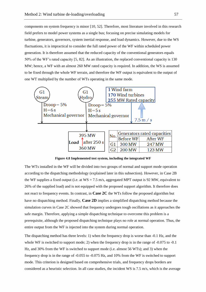
Method 2: Wind turbine de-loading/overloading 57
components on system frequency is minor [10, 52]. Therefore, most literature involved in this research
field prefers to model power systems as a single bus; focusing on precise simulating models for
turbine, generators, governors, system inertial response, and load dynamics. However, due to the WS
fluctuations, it is impractical to consider the full rated power of the WF within scheduled power
generation. It is therefore assumed that the reduced capacity of the conventional generators equals
50% of the WF‘s rated capacity [5, 82]. As an illustration, the replaced conventional capacity is 130
MW; hence, a WF with an almost 260 MW rated capacity is required. In addition, the WS is assumed
to be fixed through the whole WF terrain, and therefore the WF output is equivalent to the output of
one WT multiplied by the number of WTs operating in the same mode.
Figure 4.8 Implemented test system, including the integrated WF
The WTs installed in the WF will be divided into two groups of normal and support mode operation
according to the dispatching methodology (explained later in this subsection). However, in Case 2B
the WF supplies a fixed output (i.e. at WS = 7.5 m/s, aggregated MPT output is 92 MW, equivalent to
26% of the supplied load) and is not equipped with the proposed support algorithm. It therefore does
not react to frequency events. In contrast, in Case 2C the WTs follow the proposed algorithm but
have no dispatching method. Finally, Case 2D implies a simplified dispatching method because the
simulation curves in Case 2C showed that frequency undergoes tough oscillations as it approaches the
safe margin. Therefore, applying a simple dispatching technique to overcome this problem is a
prerequisite, although the proposed dispatching technique plays no role at normal operation. Thus, the
entire output from the WF is injected into the system during normal operation.
The dispatching method has three levels: 1) when the frequency drop is worse than -0.1 Hz, and the
whole WF is switched to support mode; 2) when the frequency drop is in the range of -0.075 to -0.1
Hz, and 30% from the WF is switched to support mode (i.e. almost 56 WTs); and 3) when the
frequency drop is in the range of -0.055 to -0.075 Hz, and 10% from the WF is switched to support
mode. This criterion is designed based on comprehensive trials, and frequency drops borders are
considered as a heuristic selection. In all case studies, the incident WS is 7.5 m/s, which is the average

Method 2: Wind turbine de-loading/overloading 58
WS in many WF locations. Moreover, AGC activation is delayed by 13 s to emphasise the influence
of the WF‘s participation in frequency deviation elimination. The same detailed modelling approach
for conventional generation that is implied in the previous chapter is applied.
The results of case studies are analysed in separate subsections where the major comments and
outcomes are summarized and discussed.
Esupport at a given WS reflects a WT‘s capability of contributing sufficiently during frequency drops
curtailment. According to Table 4.3, the maximum Esupport is achieved when the WS drops from 11 to
8.5 m/s. The applied algorithm forces the WT to keep generating power at the level reached at the
initial WS (i.e. 11 m/s in this case) for certain duration, depending on Ѡstop. This overproduction stage
depends on extracting a portion from the stored KE in the WT. In brief, the proposed algorithm
releases the full amount of extractable KE when the incident WS drops which explains why it is
preferable to run the WT at the highest allowed Ѡ. As an illustration, running the WT at high Ѡ
gives the opportunity for the WT to store more KE, which then acts as useful reserve if the WS drops
during support operation mode, so that the WT supplies the former output power for as long as
possible, regardless of the new lower WS. These outcomes reinforce the claim of the author that the
negative impact of WFs integration on system performance during frequency events is neutralized, and
even barely improved, if the WS drops during frequency recovery, although the level of improvement
depends on the severity of both the frequency excursion and WS drop.
At 5.5 m/s, the WT produces extra electrical power proportional to the available mechanical power
during support mode. The low amount of available mechanical power causes a low step rise in the
support output. Therefore, the amount of released KE is reduced, and Ѡ requires a longer time to
slow down to Ѡmin as in Figure 4.1. Nevertheless, it is possible to increase the amount of KE
extracted by setting the support electrical power to a higher value, but this can only be sustained for a
shorter time due to the rapid deterioration of Ѡ.
At 11 m/s, the WT supplies its rated output, and it is therefore theoretically unable to support the
system in the curtailment of frequency drops. Nevertheless, the overloading principle can be used as a
practical solution during such a condition. The permitted overload ratio and duration play a basic role
in determining the amount of delivered support energy. However, the amount of injected KE in this
case is almost similar to the amount of support energy when the WS is 7.5 m/s. The major advantage
in cases of high WS is the sustainability of injected energy, as it can be supplied as long as the incident
WS is high enough. Another advantage is that it avoids any slowing down of Ѡ, so that the WT
retains its normal operation directly after frequency drop clearance.

Method 2: Wind turbine de-loading/overloading 59
In general, these results do not mean that WT participation in frequency excursions is more
satisfactory if the WS drops during support mode operation. On the contrary, the proposed algorithm
targets mitigate the drawbacks of a drop in WS while the system is suffering a frequency deviation.
This problem is solved for a limited duration, which is the time consumed by the WT to inject the
available support energy. Afterwards, the system faces two possible risks, namely, a further drop in
WS or a second consecutive influential frequency deviation. If one of these two risks (or both) occurs,
the WT will be unable to offer any positive contribution in the elimination of the frequency deviation.
In other words, the presented results ensure the merits of the proposed algorithm if the incident WS
drops within a short duration just after the initiation of the frequency excursion, for example at 90 s or
longer based on WS conditions and WT specifications. This duration is considered to be critical in
eliminating a frequency drop, as most of the primary and secondary responses of conventional
generation occur within this time span, and any redundant disturbance in supplied power causes
further frequency excursions.
The tolerated frequency deviation in this case is about 0.1% of the nominal frequency (i.e. ±0.05 Hz)
[93]. A comprehensive comparison between the frequency responses of Case studies 2A to 2D is
conducted in Figure 4.9. ∆fmax, ∆f10s, tSM, and the root mean square value of ∆f within 180 s (∆fRMS) are
evaluated. These parameters clearly reflect the impact of wind energy integration on the frequency
responses in the examined cases.
The frequency curves are displayed in Figure 4.9, and the considered parameter values are gathered in
Table 4.4. It is obvious that the worst response occurred after the WF was integrated without any
support provided (Case 2B). This case has the worst ∆fRMS, ∆f10s and ∆fmax and longer tSM in
comparison with the base case. The replacement of conventional generation with a power source that
is incapable of supporting the system during frequency excursions caused these problems. However,
use of the proposed algorithm improved the performance, in particular values of ∆f10s and ∆fmax.
The fast response of the pitch controller, which switched the WF output from de-loaded condition to
optimum condition, reduced ∆fmax by 39 mHz, and ∆f10s by 13 mHz. It should be highlighted that the
WF provided a 12.42 MW power step within about 1 s, which is the time taken for the pitch angle to
drop to zero. This power step represents 34% of the load step that caused the frequency event. In
addition, this support is provided when ∆f violated the safety margin, and not immediately at the
instant of the load sudden increase. The WF provides optimum output until the ∆f enters the safe
region (i.e., the support lasts for tSM). The frequency curve suffers considerable fluctuations in Case 2C
when ∆f approaches the safe margin. As an illustration, switching the whole WF at the same time from
support mode to normal mode causes further minor frequency drops. Hence, the frequency violates the
safe margin again, thereupon the WF switches to support mode again, and thus ∆f returns back to a
safe region. This sequence is repeated until the conventional generation governor and the AGC signal
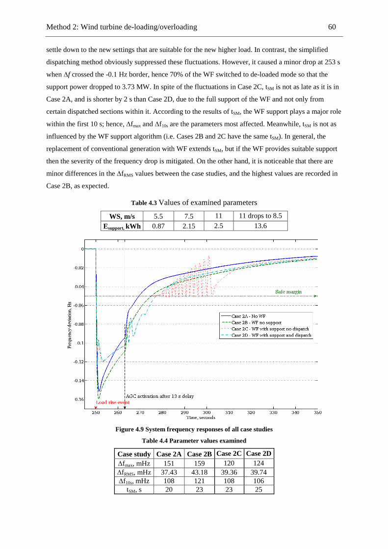
Method 2: Wind turbine de-loading/overloading 60
settle down to the new settings that are suitable for the new higher load. In contrast, the simplified
dispatching method obviously suppressed these fluctuations. However, it caused a minor drop at 253 s
when ∆f crossed the -0.1 Hz border, hence 70% of the WF switched to de-loaded mode so that the
support power dropped to 3.73 MW. In spite of the fluctuations in Case 2C, tSM is not as late as it is in
Case 2A, and is shorter by 2 s than Case 2D, due to the full support of the WF and not only from
certain dispatched sections within it. According to the results of tSM, the WF support plays a major role
within the first 10 s; hence, ∆fmax and ∆f10s are the parameters most affected. Meanwhile, tSM is not as
influenced by the WF support algorithm (i.e. Cases 2B and 2C have the same tSM). In general, the
replacement of conventional generation with WF extends tSM, but if the WF provides suitable support
then the severity of the frequency drop is mitigated. On the other hand, it is noticeable that there are
minor differences in the ∆fRMS values between the case studies, and the highest values are recorded in
Case 2B, as expected.
Table 4.3 Values of examined parameters
WS, m/s 5.5 7.5 11 11 drops to 8.5
Esupport, kWh 0.87 2.15 2.5 13.6
Figure 4.9 System frequency responses of all case studies
Table 4.4 Parameter values examined
Case study Case 2A Case 2B Case 2C Case 2D
∆fmax, mHz 151 159 120 124
∆fRMS, mHz 37.43 43.18 39.36 39.74
∆f10s, mHz 108 121 108 106
tSM, s 20 23 23 25
Method 2: Wind turbine de-loading/overloading 61
Finally, it is interesting to compare the amounts of extra energy supplied from a steam plant and a WF
within tSM. These amounts of energy are thus compared to the normal energy supplied by each source
within the same duration. The WF supplies normal energy of 82.76 MW at the given WS, which
means 574.72 kWh within tSM. In addition, it supplies 99.45 kWh of extra energy to participate in
frequency drop curtailments; hence, its contribution is 17.3% of the nominal generation within the
frequency drop high-risk period. Likewise, the steam plant participates 5.9% from its nominal
production. Consequently, the proposed algorithm gives the WF a better capability of anticipating
frequency excursions, corresponding to that of a conventional plant, particularly during its early risky
stage. Moreover, the incident WS determines the support power step magnitude and the maximum
duration within which the WT can sustain this power step.
This chapter offers a detailed algorithm for making a positive WT contribution to the elimination of
system frequency excursions. This algorithm relies on several modifications within the dominant
normal operation of a WT. In particular, three different approaches are implemented: de-loading,
overproduction, and overloading. The triggering of each technique depends on the incoming WS
according to predefined categories. Results prove that the extra supplied power is sufficient to enhance
the system performance during frequency drops. In addition, it reduces the negative impact of the WS
slowing down during support mode operation, and therefore accepted support is guaranteed regardless
of poor WS conditions. The proposed algorithm was proven to be useful when the WS immediately
fell from a certain category to a lower one, as the sudden decrease in the WS is shown to be
neutralized and does not aggravate the frequency excursion. Moreover, the proposed algorithm
partially solves the problem of wasting high amounts of wind energy using traditional de-loading
techniques, by the continuous operation of the WT in de-loaded mode, because the de-loaded
operation is activated only at certain WS category. Implementing the proposed algorithm on a
hypothetical system showed a clear enhancement of system performance during its recovery from a
moderate frequency deviation. In addition, a comparison of the contributions between a WF and a
conventional generator reflected the WF efficient contribution.

Comparison of proposed support methods 62
The supportive role of WTs during frequency drops proposed by many algorithms causes the WT to
deviate from delivering optimum power generation. Special operational methods drive the WT to
guarantee the availability of reasonable power support when the system suffers frequency deviations.
This chapter compares the two algorithms offered, as well as the standard de-loading technique widely
proposed in literature. Wind turbine power curves for each algorithm are then derived, and a
comparison is conducted from the point of view of wasted energy with respect to optimum power
generation operation. This analysis is performed in two locations that are considered to be promising
candidates for WFs construction in Egypt, and uses an integration of two different types of WTs.
The WT output power depends on three variable parameters; rotational speed, WS, and pitch angle, as
illustrated before in Subsections (2.1) and (2.3). Consequently, the optimum tip speed ratio that
achieves an optimum Cp of each WT type is determined. The WT rotational speed is adjusted so that
Cp tracks its optimum value at all times. This constraint is fulfilled by continually adjusting the value
of rotational speed so as to maintain the optimum tip speed at all WSs. The question now is how to
simulate the estimation of the optimum power value at each WS according to MPT operation. This
chapter represents two different approaches for obtaining WT performance curves that fulfil the MPT.
The WT fabricating company provides a standard power curve for each WT type where the WT output
at each WS is indicated within a margin between WSCI and WSCO. These power values are based on
continuous monitoring for WT performance, and are the average of several records taken at each WS.
The power curve data can then be manipulated into a lookup table using an appropriate interpolation
method; hence, the optimum WT output can be estimated at any WS. The most critical region in this
curve is between WSCI and WSR, elsewhere the output is rated (i.e. 1 pu), or zero, according to the
WS.
This method aims to minimize possible errors in MPT 1, and relies mainly on the WT model and Cp
equation constants. It is well known that a variable speed WT has a certain range of rotor speeds that
are predetermined by the manufacturer. Therefore, the control algorithm derived for the WT should
not violate these limits by any means in order to avoid any possible loss of synchronism or physical
damage. In this proposed algorithm, the output power at a certain WS is evaluated using (2.1) and
(2.3) at all feasible rotor speeds. Thus, the maximum (i.e. optimum) possible output power is
determined at each WS starting from WSCI until WSR. However, the step between two successive WSs
(i.e. the WS class; for example if the WS class equals 0.5 m/s the examined WSs are WSCI + 0.5, WSCI

Comparison of proposed support methods 63
+ 2×0.5, WSCI+ 3×0.5,…., WSR+ 0.5) contributes to the accuracy of the obtained look-up table. In
other words, reducing the WS class mitigates the role of the applied interpolation method, thus
reducing error. Illustrative Figures are provided in Subsection 5.5, based on the considered case
studies.
It should be highlighted that application of the MPT algorithm makes the WT incapable of providing
additional active power support during frequency excursions. However, alternative solutions depend
on energy storage mediums, as discussed later in Chapter 8.
This section briefly explains the WT‘s operation during over-speeding (Method 1), de-loading, and the
proposed innovative partial de-loading support technique (Method 2). In addition, it explains the
method used to construct the WT performance curves in normal operation according to each
algorithm.
As mentioned before, the contribution of a WT in frequency drop curtailments may rely on the amount
of stored KE in its rotating parts. The algorithm offered in Chapter 3 maintains a higher value for the
tip speed ratio, hence the rotor speed increases, and in turn, the available KE is enlarged. In particular,
λH evaluated in (3.3) is applied. In sequence, the WS, rotor speed, and pitch angle are used to estimate
WT output using (2.1) to (2.3). It is of note that over-speeding is valid only in the range of (WSCI <
WS < WSR). As an illustration, starting from WSR the WT operates around its maximum rotor speed,
thus it is unable to cause the WT to over-speed or to violate the rotor speed limits.
A WT is operated so that the WT output is less than the optimum available power. Thus, the deficit
between the actual output power and the optimum output is considered as a strategic reserve to support
the system during frequency deviations. As mentioned in Subsection 2.3.2, de-loading can be applied,
mainly by using two techniques:
Running the WT at a rotational speed higher than the optimum speed (note that the
optimum speed is the speed which leads to λ = λo). This method is called WT over-
speeding.
Activating pitch control at all WSs so that the output is reduced according to the implied
pitch angle. This technique is applicable for any WT equipped with pitch angle controls.
However, pitching is a slower alternative due to the mechanical response of servo motors
controlling each blade pitch angle.

Comparison of proposed support methods 64
In both techniques, a predefined de-loading factor (DF) is selected by SOs according to their
requirements of the WFs contribution to mitigating frequency drops. In this chapter, DF= 15% and the
minor differences between the two sub-techniques are ignored (i.e. WT de-loaded generated power is
the same in both sub-techniques).
The major merits and uniqueness of this algorithm appear in three factors: 1) it is adapted with the WT
and WS conditions within the WF location; 2) the de-loading is activated only within certain ranges of
WS, as explained in Subsection 4.1.1 (de-loading is applied in the following conditions: 1) WSlow<
WS < WSR and 2) normal PWTm is less than 1 pu; and 3) its capability of handling WS drops
intersecting with frequency events, thereby reducing the negative impact of such sudden dips in WS.
This section explains the method used to estimate the amount of generated energy by a WT within a
certain time span, according to a given chronological WS array. These energies are estimated to judge
how much energy is wasted in the discussed frequency support algorithms. WS chronological arrays in
certain locations are considered as an input to the constructed look-up tables, so that the amount of
generated wind energies within the concerned time spectrum is estimated using 5.1 to 5.4 (i.e. WS
chronological array must be available within a considered interval). EMPT1 and EMPT2 stand for
generated energies within a considered time span (T), when the WT operates based on MPT through
the methods explained in Subsections 5.1.1 and 5.1.2 respectively. EOS, ED, and EPD stand for the
generated energies when the WT operates using over-speeding, de-loaded, and partially de-loaded
strategies, respectively. The time step (i.e., time duration between each two successive WS records) of
the available chronological WS array is tWS, and N is the number of WS records within T. WT output
is evaluated based on the performance curves of the WT type and the acknowledged operation
algorithm. However, the transients occurring during the shift from one WS to another are ignored
because they have a minor impact on the overall energy generated. Generally, energy is the integration
of power during time. As the time deficit between each two successive WS records is fixed (i.e. tWS),
the energy produced at each WS record is equivalent to the product of PWTm and tWS. Meanwhile,
PWTm is de-loaded all the time in a continuous de-loading operation; hence it equals ‗PWTm· DF‘.
Consequently, equation (5.2) is valid. The amount of wasted energy is calculated with correspondence
to EMPT2, for example the difference between EMPT2 and ED represents the wasted energy due to
integration of the continuous de-loading algorithm.
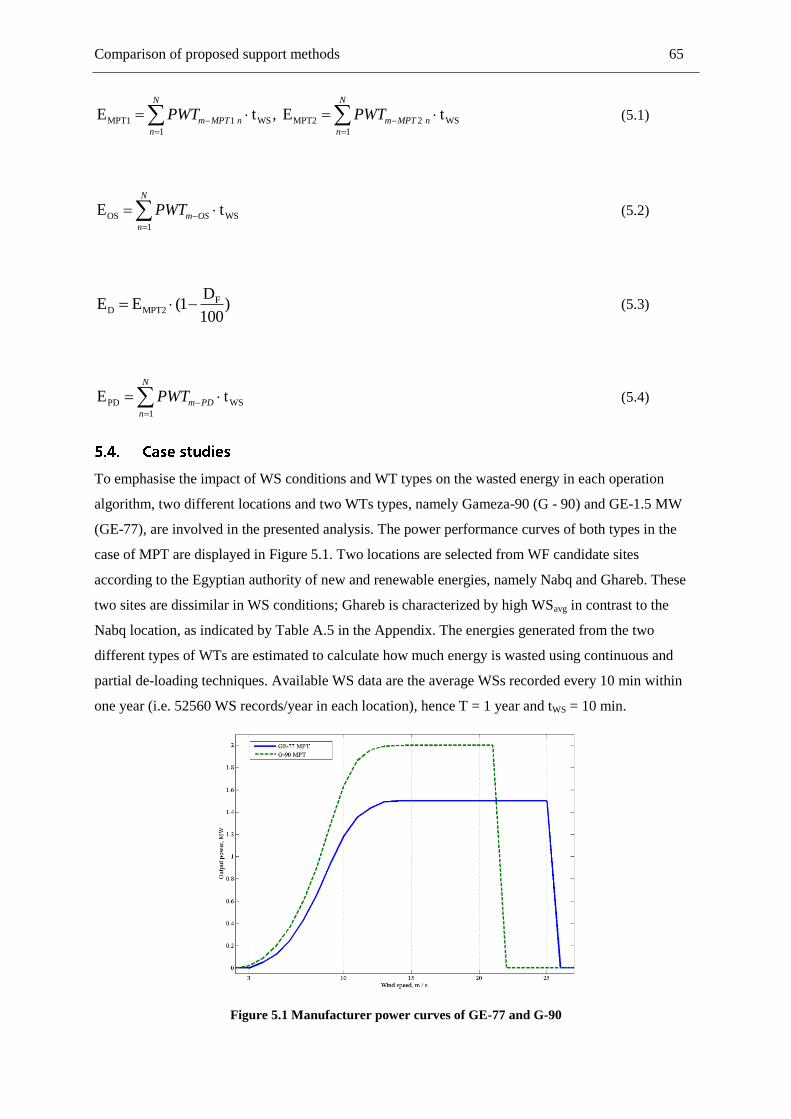
Comparison of proposed support methods 65
MPT1 1 WS MPT2 2 WS
1 1
E t , E tN N
m MPT n m MPT n
n n
PWT PWT
(5.1)
OS WS
1
E tN
m OS
n
PWT
(5.2)
FD MPT2
DE E (1 )
100 (5.3)
PD WS
1
E tN
m PD
n
PWT
(5.4)
To emphasise the impact of WS conditions and WT types on the wasted energy in each operation
algorithm, two different locations and two WTs types, namely Gameza-90 (G - 90) and GE-1.5 MW
(GE-77), are involved in the presented analysis. The power performance curves of both types in the
case of MPT are displayed in Figure 5.1. Two locations are selected from WF candidate sites
according to the Egyptian authority of new and renewable energies, namely Nabq and Ghareb. These
two sites are dissimilar in WS conditions; Ghareb is characterized by high WSavg in contrast to the
Nabq location, as indicated by Table A.5 in the Appendix. The energies generated from the two
different types of WTs are estimated to calculate how much energy is wasted using continuous and
partial de-loading techniques. Available WS data are the average WSs recorded every 10 min within
one year (i.e. 52560 WS records/year in each location), hence T = 1 year and tWS = 10 min.
Figure 5.1 Manufacturer power curves of GE-77 and G-90
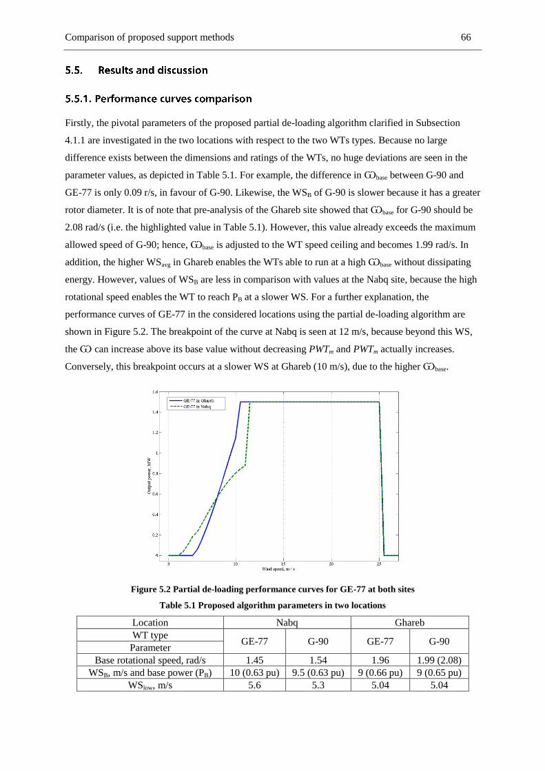
Comparison of proposed support methods 66
Firstly, the pivotal parameters of the proposed partial de-loading algorithm clarified in Subsection
4.1.1 are investigated in the two locations with respect to the two WTs types. Because no large
difference exists between the dimensions and ratings of the WTs, no huge deviations are seen in the
parameter values, as depicted in Table 5.1. For example, the difference in Ѡbase between G-90 and
GE-77 is only 0.09 r/s, in favour of G-90. Likewise, the WSB of G-90 is slower because it has a greater
rotor diameter. It is of note that pre-analysis of the Ghareb site showed that Ѡbase for G-90 should be
2.08 rad/s (i.e. the highlighted value in Table 5.1). However, this value already exceeds the maximum
allowed speed of G-90; hence, Ѡbase is adjusted to the WT speed ceiling and becomes 1.99 rad/s. In
addition, the higher WSavg in Ghareb enables the WTs able to run at a high Ѡbase without dissipating
energy. However, values of WSB are less in comparison with values at the Nabq site, because the high
rotational speed enables the WT to reach PB at a slower WS. For a further explanation, the
performance curves of GE-77 in the considered locations using the partial de-loading algorithm are
shown in Figure 5.2. The breakpoint of the curve at Nabq is seen at 12 m/s, because beyond this WS,
the Ѡ can increase above its base value without decreasing PWTm and PWTm actually increases.
Conversely, this breakpoint occurs at a slower WS at Ghareb (10 m/s), due to the higher Ѡbase.
Figure 5.2 Partial de-loading performance curves for GE-77 at both sites
Table 5.1 Proposed algorithm parameters in two locations
Location Nabq Ghareb
WT type GE-77 G-90 GE-77 G-90
Parameter
Base rotational speed, rad/s 1.45 1.54 1.96 1.99 (2.08)
WSB, m/s and base power (PB) 10 (0.63 pu) 9.5 (0.63 pu) 9 (0.66 pu) 9 (0.65 pu)
WSlow, m/s 5.6 5.3 5.04 5.04
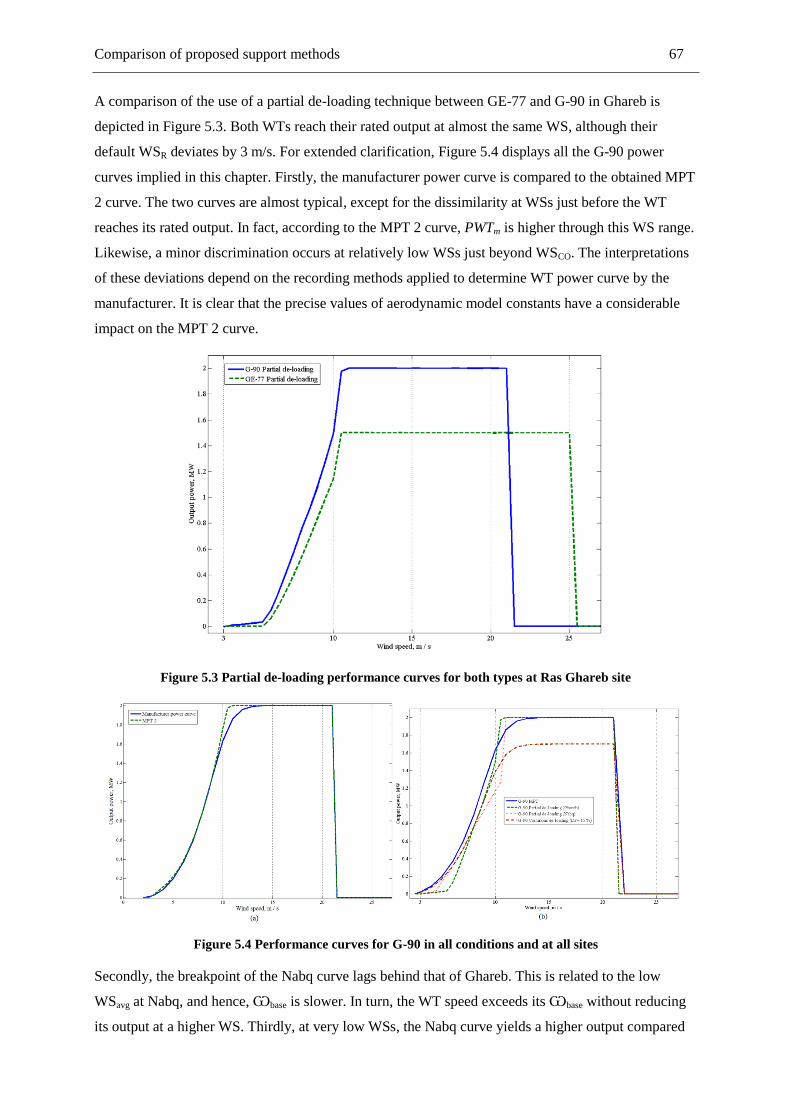
Comparison of proposed support methods 67
A comparison of the use of a partial de-loading technique between GE-77 and G-90 in Ghareb is
depicted in Figure 5.3. Both WTs reach their rated output at almost the same WS, although their
default WSR deviates by 3 m/s. For extended clarification, Figure 5.4 displays all the G-90 power
curves implied in this chapter. Firstly, the manufacturer power curve is compared to the obtained MPT
2 curve. The two curves are almost typical, except for the dissimilarity at WSs just before the WT
reaches its rated output. In fact, according to the MPT 2 curve, PWTm is higher through this WS range.
Likewise, a minor discrimination occurs at relatively low WSs just beyond WSCO. The interpretations
of these deviations depend on the recording methods applied to determine WT power curve by the
manufacturer. It is clear that the precise values of aerodynamic model constants have a considerable
impact on the MPT 2 curve.
Figure 5.3 Partial de-loading performance curves for both types at Ras Ghareb site
Figure 5.4 Performance curves for G-90 in all conditions and at all sites
Secondly, the breakpoint of the Nabq curve lags behind that of Ghareb. This is related to the low
WSavg at Nabq, and hence, Ѡbase is slower. In turn, the WT speed exceeds its Ѡbase without reducing
its output at a higher WS. Thirdly, at very low WSs, the Nabq curve yields a higher output compared

Comparison of proposed support methods 68
to that of Ghareb, but this situation is reversed at medium WSs. As an illustration, the de-loaded
operation parameters are adapted for lower WSavg in Nabq. Finally, MPT and the continuous de-loaded
curves are typical in attitude. However, MPT is only reduced by DF factor to produce the power curve
of continuous de-loaded operation (e.g. rated output is de-loaded to 1.7 MW).
The generated electrical energy over one year (i.e. according to available WS arrays in each location)
from one WT in all cases is gathered in Table 5.2. The results show that the MPT 2 curve reveals
better operational points for a WT, which is why EMPT2 is higher than EMPT1 in all cases. Nevertheless,
the deviations between the two values fluctuate according to the WT type and WS nature in the
considered locations. In particular, Ghareb has better WS conditions compared to Nabq, hence the
impact of the difference between MPT2 and the standard power curve increases (i.e., in Nabq EMPT2 is
higher by 270 MWh compared to 380 MWh in Ghareb). Although the rating of G-90 is more than GE-
77, the difference between EMPT2 and EMPT1 in Ghareb is higher in favour of the GE-77, by 200 MWh.
This could be justified by the accuracy and the nature of aerodynamic models of both WT types.
Implementation of the over-speeding technique causes less energy to be wasted, (refer to Table 5.2
and Figure 5.5). This merit is achieved by the over-speeding technique because 1) it reduces PWTm by
a small margin; and 2) it has a limited activation range compared to the continuous de-loading
technique (i.e., over-speeding is valid only for WSCI < WS < WSR). However, the provided active
power support from this algorithm is less compared to that of the other two methods, and it depends
completely on the amount of extracted KE.
Additionally, this algorithm must decelerate the rotor speed during frequency deviations clearance,
which increases the rate of usage of the electronic converters and the risk of loss of synchronism.
Moreover, the rotor speed needs to recover its default value after the support period, thus PWTm is
reduced to allow rotor speed acceleration until it again reaches the height of the tip speed ratio.
However, EPD is more than ED in all cases. At the Ghareb site (with GE-77 installed), the partial de-
loading technique wasted only 7.5% with respect to EMPT2, compared to 21% wasted by the continuous
de-loading method. However, the advantage of partial de-loading is reduced in Nabq, as continuous
de-loading wasted 21.9% while partial de-loading wasted 21.4%. This might be seen as trivial, but if
the price of kWh based on Egyptian tariffs is acknowledged, it means that a single WT wastes about
2390 € annually when it is continuously de-loaded (0.5% x 4.78 GWh x 0.1 €/kWh). This value is
enormous if multiplied by the number of WTs in each WF.
Table 5.2 Amounts of annual generated energy (GWh) for each operational algorithm
Location Ghareb Nabq Annual energy production, GWh
EMPT1 EMPT2 EPD ED EOS EMPT1 EMPT2 EPD ED EOS WT type GE-77 8.63 9.21 8.5 7.34 9 4.78 5.21 4.09 4.07 5 G-90 11.77 12.15 11.35 10 12 6.63 6.9 5.78 5.63 6.9
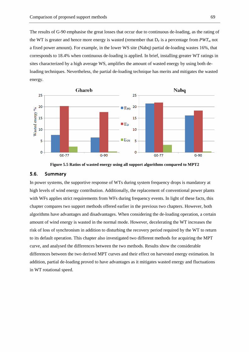
Comparison of proposed support methods 69
The results of G-90 emphasise the great losses that occur due to continuous de-loading, as the rating of
the WT is greater and hence more energy is wasted (remember that DF is a percentage from PWTm not
a fixed power amount). For example, in the lower WS site (Nabq) partial de-loading wastes 16%, that
corresponds to 18.4% when continuous de-loading is applied. In brief, installing greater WT ratings in
sites characterized by a high average WS, amplifies the amount of wasted energy by using both de-
loading techniques. Nevertheless, the partial de-loading technique has merits and mitigates the wasted
energy.
Figure 5.5 Ratios of wasted energy using all support algorithms compared to MPT2
In power systems, the supportive response of WTs during system frequency drops is mandatory at
high levels of wind energy contribution. Additionally, the replacement of conventional power plants
with WFs applies strict requirements from WFs during frequency events. In light of these facts, this
chapter compares two support methods offered earlier in the previous two chapters. However, both
algorithms have advantages and disadvantages. When considering the de-loading operation, a certain
amount of wind energy is wasted in the normal mode. However, decelerating the WT increases the
risk of loss of synchronism in addition to disturbing the recovery period required by the WT to return
to its default operation. This chapter also investigated two different methods for acquiring the MPT
curve, and analysed the differences between the two methods. Results show the considerable
differences between the two derived MPT curves and their effect on harvested energy estimation. In
addition, partial de-loading proved to have advantages as it mitigates wasted energy and fluctuations
in WT rotational speed.
Wind farm energy production assessment– an Egyptian case study 70
This chapter investigates a critical problem in relation to the estimation of the average expected wind
energy production and penetration level in a given power system. This issue has a deep influence on
system frequency response and the expected performance during frequency excursions. This chapter
therefore presents an innovative method, based on the algorithm discussed in the Chapter 4 of
evaluating the amount of conventional generation that could be replaced by certain WFs. This
evaluation depends on the WS prospects in each WF location as well as the implied operation
algorithm in the integrated WTs. Additionally, the types and specifications of installed WTs in each
WF have a considerable impact on such analysis, hence all details need to be considered to ensure
better accuracy of the obtained results. The practical application of the proposed method of assessment
is then conducted on the Egyptian case.
The considered replacement of conventional units is directly related to the forecasted annual energy
production of the WF. Some literature assume that a WF should be able to generate an annual average
value of 40% from its aggregated rated power capacity due to the intermittent nature of WS, and this
has already been applied in the two previous chapters [80, 90]. However, a simplified innovative
method to estimate the actual WFs capacities is also proposed, although the lack of geographical data
concerning the area of suitable land at each proposed WF site forced the author to apply two certain
assumptions. Firstly, all WFs have the same number of WTs; 100 WTs. Secondly, the shadowing and
tower effects on WS propagation through the WF is interpreted by an overall reduction of 10% of the
WF‘s overall annual produced energy, and this de-rating ratio is inspired from the results obtained in
[87].
Three modern types of WTs of various sizes and ratings: Enercon 101–3.05 MW, Nordex 117–2.4
MW, and Gameza 90–2 MW, are integrated in this chapter. The main technical data related to each are
summarized in Table A.1 in the Appendix [21, 94, 95]. The integration of several types of WTs
emphasises the influence of the proposed method on the current state of wind energy expansion.
Although, it is essential to apply relatively accurate models for the considered WTs, it is difficult to
gain access to the technical specifications of manufacturer‘s models of integrated WTs. Hence the
author coefficients values found in [18] are implemented. These generic models have the same
structure of the accredited generic model of GE-77 embedded in the Simulink power system library.
However, the constant values alter according to the considered WT type, and these values are found in
Appendix 11.2. The outcomes of the energy production assessment procedure are utilized to match
3 The major content of this chapter is published in IEEE 4th International conference on power engineering and energy as
indicated in Related publications list
Wind farm energy production assessment– an Egyptian case study 71
both the WT types and the location of the WFs, keeping in mind a homogeneous distribution of the
presence of three types of WTs among the considered locations.
The annual available energy produced by each WF, founded on WS records in a WF location, is the
concept used for the presented assessment procedure. For instance, the annual energy produced by
each WT at each site is calculated in relation to the assigned operation algorithm that was offered in
Chapter 4. It is of note that this assessment procedure assumes no wind energy rejection (i.e. all the
available wind power is fed to the intended grid).
According to Method 2, three critical values are evaluated at each site for each WT type: WSlow,
WSrated and Ѡb. For simplicity, WSCI is assumed to be similar for all WT types and equals 4 m/s.
These three major values are calculated as explained in Subsection 4.1.1. It is important to mention
that de-loading techniques are suspended in this chapter to prevent any energy losses caused by de-
loading. Thus, the highest wind energy production is estimated. Early trials to simulate the output
power of each WT model at each location during the whole year in seconds (31,536,000s) required
tremendous computational efforts and storage capacity, in addition to the extremely long execution
time involved. Therefore, a minor approximation is applied to evaluate the expected annual wind
energy production using reduced computational efforts. However, this algorithm retains an acceptable
level of accuracy and does not ignore the produced energy within WT transients during WS
transitions.
Firstly, the WS records need refining, and the time span between each two successive readings is
identified (tWS) in seconds so that each WF location has its own array(s) of WS records. Sometimes, a
single WF has more than one WS array because the WS is inspected in different regions across the WF
area. Thus, the presented procedure is repeated in each region, taking into consideration the possible
(or the intended) number of WTs that should be installed in the region. tWS is divided into two
intervals: the first 25 s within which WT transients occurs due to the WS shifting to a new value (the
integral part of equation 6.1) and the second is (tWS – 25), where PWTm is assumed to be constant
(transients stabilize) and equals the last value reached in the first interval (i.e. PWTm (WSi, 25) where i
= 1 to 52560). The instantaneous PWTm array is obtained using the Simulink WT model operated by
Method 2, using the continuous time domain simulation. In other words, the energy generated at a
certain WS reading number ‗i‘ starting at time = ti and continuing for t = ti + tWS, is obtained using
(6.1). This equation also emphasises how the output power array is obtained. This process is repeated
(31536000/tWS) times to obtain the overall generated annual energy by a given WT type in a certain
WF location.
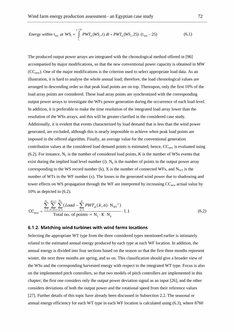
Wind farm energy production assessment– an Egyptian case study 72
25
i WS t WS ( , ) ( ,25) (t 25)i
i
t
WS m i m i
t
Energy within at PWT WS t dt PWT WS
(6.1)
The produced output power arrays are integrated with the chronological method offered in [96]
accompanied by major modifications, so that the new conventional power capacity is obtained in MW
(CCnew). One of the major modifications is the criterion used to select appropriate load data. As an
illustration, it is hard to analyse the whole annual load; therefore, the load chronological values are
arranged in descending order so that peak load points are on top. Thereupon, only the first 10% of the
load array points are considered. These load array points are synchronized with the corresponding
output power arrays to investigate the WFs power generation during the occurrence of each load level.
In addition, it is preferable to make the time resolution of the integrated load array lower than the
resolution of the WSs arrays, and this will be greater-clarified in the considered case study.
Additionally, it is evident that events characterized by load demand that is less than the wind power
generated, are excluded, although this is nearly impossible to achieve when peak load points are
imposed in the offered algorithm. Finally, an average value for the conventional generation
contribution values at the considered load demand points is estimated; hence, CCnew is evaluated using
(6.2). For instance, NL is the number of considered load points, K is the number of WSs events that
exist during the implied load level number (i). Np is the number of points in the output power array
corresponding to the WS record number (k), X is the number of connected WFs, and NWT is the
number of WTs in the WF number (x). The losses in the generated wind power due to shadowing and
tower effects on WS propagation through the WF are interpreted by increasing CCnew actual value by
10% as depicted in (6.2).
pL
NN ( )
WT1 1( ) 1 1
new
L p
( ( , ) N )
CC 1.1Total no. of points = N K N
K i Xx
i mi k i n x
Load PWT k n
(6.2)
Selecting the appropriate WT type from the three considered types mentioned earlier is intimately
related to the estimated annual energy produced by each type at each WF location. In addition, the
annual energy is divided into four sections based on the season so that the first three months represent
winter, the next three months are spring, and so on. This classification should give a broader view of
the WSs and the corresponding harvested energy with respect to the integrated WT type. Focus is also
on the implemented pitch controllers, so that two models of pitch controllers are implemented in this
chapter; the first one considers only the output power deviation signal as an input [26], and the other
considers deviations of both the output power and the rotational speed from their reference values
[27]. Further details of this topic have already been discussed in Subsection 2.2. The seasonal or
annual energy efficiency for each WT type in each WF location is calculated using (6.3), where 8760
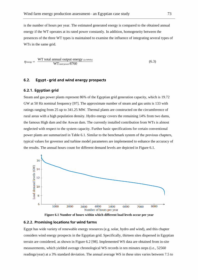
Wind farm energy production assessment– an Egyptian case study 73
is the number of hours per year. The estimated generated energy is compared to the obtained annual
energy if the WT operates at its rated power constantly. In addition, homogeneity between the
presences of the three WT types is maintained to examine the influence of integrating several types of
WTs in the same grid.
(in MWhr)energy
rated power
WT total annual output energy
WT 8760
(6.3)
Steam and gas power plants represent 86% of the Egyptian grid generation capacity, which is 19.72
GW at 50 Hz nominal frequency [97]. The approximate number of steam and gas units is 133 with
ratings ranging from 25 up to 341.25 MW. Thermal plants are constructed on the circumference of
rural areas with a high population density. Hydro energy covers the remaining 14% from two dams,
the famous High dam and the Aswan dam. The currently installed contribution from WTs is almost
neglected with respect to the system capacity. Further basic specifications for certain conventional
power plants are summarized in Table 6.1. Similar to the benchmark system of the previous chapters,
typical values for governor and turbine model parameters are implemented to enhance the accuracy of
the results. The annual hours count for different demand levels are depicted in Figure 6.1.
Figure 6.1 Number of hours within which different load levels occur per year
Egypt has wide variety of renewable energy resources (e.g. solar, hydro and wind), and this chapter
considers wind energy prospects in the Egyptian grid. Specifically, thirteen sites dispersed in Egyptian
terrain are considered, as shown in Figure 6.2 [98]. Implemented WS data are obtained from in-site
measurements, which yielded average chronological WS records in ten minutes steps (i.e., 52560
readings/year) at a 3% standard deviation. The annual average WS in these sites varies between 7.5 to
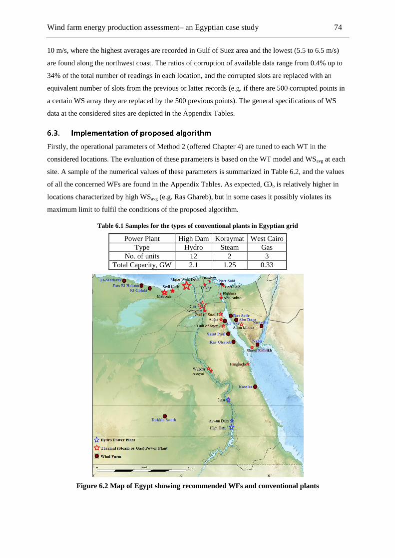
Wind farm energy production assessment– an Egyptian case study 74
10 m/s, where the highest averages are recorded in Gulf of Suez area and the lowest (5.5 to 6.5 m/s)
are found along the northwest coast. The ratios of corruption of available data range from 0.4% up to
34% of the total number of readings in each location, and the corrupted slots are replaced with an
equivalent number of slots from the previous or latter records (e.g. if there are 500 corrupted points in
a certain WS array they are replaced by the 500 previous points). The general specifications of WS
data at the considered sites are depicted in the Appendix Tables.
Firstly, the operational parameters of Method 2 (offered Chapter 4) are tuned to each WT in the
considered locations. The evaluation of these parameters is based on the WT model and WSavg at each
site. A sample of the numerical values of these parameters is summarized in Table 6.2, and the values
of all the concerned WFs are found in the Appendix Tables. As expected, Ѡb is relatively higher in
locations characterized by high WSavg (e.g. Ras Ghareb), but in some cases it possibly violates its
maximum limit to fulfil the conditions of the proposed algorithm.
Table 6.1 Samples for the types of conventional plants in Egyptian grid
Power Plant High Dam Koraymat West Cairo
Type Hydro Steam Gas
No. of units 12 2 3
Total Capacity, GW 2.1 1.25 0.33
Figure 6.2 Map of Egypt showing recommended WFs and conventional plants

Wind farm energy production assessment– an Egyptian case study 75
Therefore, Ѡb is adjusted to its maximum value; the highlighted values represent the examples of
such cases. This problem appears only with N-117 and E-101, as they have a lower maximum limit for
Ѡb in comparison with G-90.
The second step is to generate the output power arrays for the three WTs in all locations, as explained
earlier. The instantaneous output power of some WTs in some locations, and the corresponding WSs,
are displayed in Figure 6.3. The energy efficiency of each WT type in each location is then evaluated,
as explained in Subsection 6.1.2. A sample of the obtained results is presented in Table 6.3 and Figure
6.4, and the complete results are included in the Appendix Tables. According to these outcomes, N-
117 has the best record at all sites due to its aerodynamics characteristics, which serve to obtain a
higher output power at lower WSs. In light of the evaluated ηenergy, WT types are matched with WF
locations. However, the same type of WT is not integrated in more than five locations to guarantee a
homogeneous mix between WT types and locations. The final allocation of WT types is found in
Table 6.4.
The next step is to calculate CCnew in relation to the Egyptian grid annual load and available WFs
output power arrays. The available Egyptian grid annual load is in the form of 1 h steps, and the WS
records are in 10 min steps. Thus, the WS has six different values during each load step. However, the
annual load array points are arranged in descending order, and only 10% are included in CCnew
evaluation.
Table 6.2 Ѡb, WSbase and WSrated at certain WF sites
WT Location (WSavg) El-Mathany (5.75) Ras Elhekma (6.52)
WT model E-101 G-90 N-117 E-101 G-90 N-117
Ѡb (rad./s) 0.9 1.3 1.0 1.0 1.5 1.1
WSrated (m/s) 16.9 15.8 9.6 14.6 12.4 10.1
WSbase (m/s) 15.0 14.0 8.5 13.0 11.0 9.0
WT Location(WSavg) Ras Ghareb (9.77) Saint Paul (8.25)
WT model E-101 G-90 N117 E-101 G-90 N-117
Ѡb (rad./s) 1.5 1.7 1.4 1.3 1.6 1.4
WSrated (m/s) 11.0 11.3 9.6 11.3 11.8 9.6
WSbase (m/s) 9.8 10.0 8.5 10.0 10.5 8.5
The Egyptian grid load levels and their corresponding durations of occurrence are depicted in Figure
6.1. For instance, each WF is aggregated as one single WT, so that the WT output array is multiplied
by the number of WTs inside the WF (i.e., 100 WTs in this study). The power arrays of WFs are
synchronized with the time span at which the load point (i) occurs.
For example, the maximum load point (i.e., 17.3 GW) occurring at hour number 7663 is equivalent to
the WS readings starting from record number 45978 (7663·6) to 45983 (7663·6 + 5). Thus, each load
time span includes 6 different WSs (k=1 to 6). The value of parameters used in (6.2) are K = 6, NL =
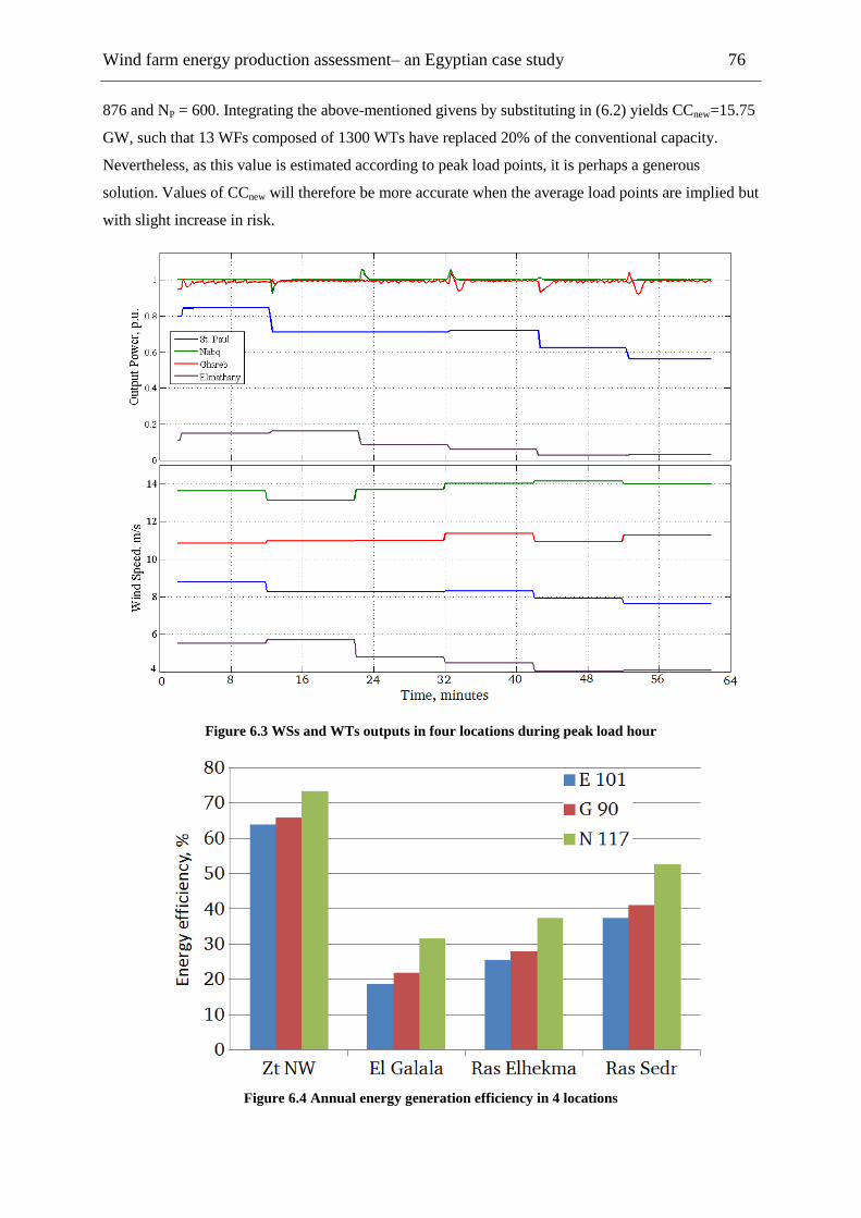
Wind farm energy production assessment– an Egyptian case study 76
876 and NP = 600. Integrating the above-mentioned givens by substituting in (6.2) yields CCnew=15.75
GW, such that 13 WFs composed of 1300 WTs have replaced 20% of the conventional capacity.
Nevertheless, as this value is estimated according to peak load points, it is perhaps a generous
solution. Values of CCnew will therefore be more accurate when the average load points are implied but
with slight increase in risk.
Figure 6.3 WSs and WTs outputs in four locations during peak load hour
Figure 6.4 Annual energy generation efficiency in 4 locations

Wind farm energy production assessment– an Egyptian case study 77
Table 6.3 Seasonal energy in GWh and ηenergy in % in certain locations
Location ZT NW (10 m/s) El-Galala (6 m/s) Ras Sedr (7.4 m/s)
Season/WT E-101 G-90 N-117 E-101 G-90 N-117 E-101 G-90 N-117
Winter Energy 5.8 3.9 4.9 1.1 0.8 1.4 3.5 2.5 3.8
ηenergy 87.3 88.1 94.0 15.9 18.2 27.1 53.1 57.9 71.4
Spring Energy 4.6 3.1 4.1 1.1 0.8 1422.3 2.6 1.9 2.9
ηenergy 68.7 71.0 78.2 15.9 18.6 27.1 39.3 43.3 55.1
Summer Energy 2.3 1.7 2.5 1.6 1.3 2152.7 1.2 0.9 1.6
ηenergy 34.1 37.8 47.7 24.5 28.8 41.0 17.6 20.3 30.3
Fall Energy 4.4 2.9 3.9 1.3 0.9 1.6 2.6 1.9 2.8
ηenergy 65.4 66.8 73.4 18.7 21.4 30.9 39.4 42.8 53.5
Table 6.4 Final matching of WTs to 13 considered wind farms sites
Location WT type
Location WT type
Abu Dara E-101
Nweiba N-117
Dakhla E-101
Port Said G-90
El-Galala N-117
Ras El-Hekma G-90
El-Mathany G-90
Ras Ghareb G-90
Kossier N-117
Ras Sedr N-117
Nabq E-101 St. Paul N-117
NW ZT E-101
The system frequency response is examined before and after wind energy penetration through a
continuous time domain simulation. To achieve this target, the construction of a test system is required
that represents the main features of the Egyptian grid that have a direct impact on the frequency
response. According to [10, 52], the modelling of transmission lines and transformers is minor and
does not have a deep impact on frequency stability studies. Therefore, the implemented test system
highlights in detail the conventional generators and connected WFs. The model includes complete
models of hydro-, steam, and gas generators, as well as their governors. The models of the governors
are similar to those used earlier in Chapters 3 and 4. For simplicity, it is assumed that each
conventional generation technology is presented by one aggregated power plant that has a contribution
of CCnew, which is proportional to its real ratio in the Egyptian grid. For example, hydro generation
participates 14%, hence the hydro generator capacity before wind integration is 2.76 GW (i.e.,
14%·19.7 = 2.76 GW) and after the connection of WFs is 2.2 GW. Similarly, the thermal generation
capacity is split into 75% steam and 25% gas power plants. Consequently, the steam generation
capacity before and after the WFs are connected is 12.7 and 10.16 GW, respectively. A single line
diagram of the implemented test system is shown in Figure 6.5, taking into consideration the
integrated WFs described in Table 6.4, where each WF is composed of 100 WTs of the above-
mentioned types. The wake and shadowing effects are ignored in this chapter. During simulation, the
power references of conventional generators governors are adjusted continuously based on the WFs
changing outputs as in (6.4):
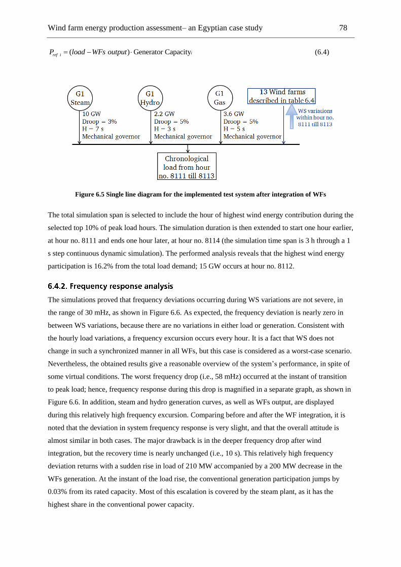
Wind farm energy production assessment– an Egyptian case study 78
( ) Generator Capacityiref iP load WFs output (6.4)
Figure 6.5 Single line diagram for the implemented test system after integration of WFs
The total simulation span is selected to include the hour of highest wind energy contribution during the
selected top 10% of peak load hours. The simulation duration is then extended to start one hour earlier,
at hour no. 8111 and ends one hour later, at hour no. 8114 (the simulation time span is 3 h through a 1
s step continuous dynamic simulation). The performed analysis reveals that the highest wind energy
participation is 16.2% from the total load demand; 15 GW occurs at hour no. 8112.
The simulations proved that frequency deviations occurring during WS variations are not severe, in
the range of 30 mHz, as shown in Figure 6.6. As expected, the frequency deviation is nearly zero in
between WS variations, because there are no variations in either load or generation. Consistent with
the hourly load variations, a frequency excursion occurs every hour. It is a fact that WS does not
change in such a synchronized manner in all WFs, but this case is considered as a worst-case scenario.
Nevertheless, the obtained results give a reasonable overview of the system‘s performance, in spite of
some virtual conditions. The worst frequency drop (i.e., 58 mHz) occurred at the instant of transition
to peak load; hence, frequency response during this drop is magnified in a separate graph, as shown in
Figure 6.6. In addition, steam and hydro generation curves, as well as WFs output, are displayed
during this relatively high frequency excursion. Comparing before and after the WF integration, it is
noted that the deviation in system frequency response is very slight, and that the overall attitude is
almost similar in both cases. The major drawback is in the deeper frequency drop after wind
integration, but the recovery time is nearly unchanged (i.e., 10 s). This relatively high frequency
deviation returns with a sudden rise in load of 210 MW accompanied by a 200 MW decrease in the
WFs generation. At the instant of the load rise, the conventional generation participation jumps by
0.03% from its rated capacity. Most of this escalation is covered by the steam plant, as it has the
highest share in the conventional power capacity.
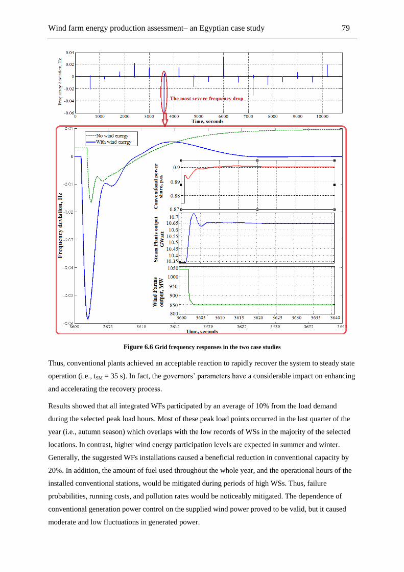
Wind farm energy production assessment– an Egyptian case study 79
Figure 6.6 Grid frequency responses in the two case studies
Thus, conventional plants achieved an acceptable reaction to rapidly recover the system to steady state
operation (i.e., tSM = 35 s). In fact, the governors‘ parameters have a considerable impact on enhancing
and accelerating the recovery process.
Results showed that all integrated WFs participated by an average of 10% from the load demand
during the selected peak load hours. Most of these peak load points occurred in the last quarter of the
year (i.e., autumn season) which overlaps with the low records of WSs in the majority of the selected
locations. In contrast, higher wind energy participation levels are expected in summer and winter.
Generally, the suggested WFs installations caused a beneficial reduction in conventional capacity by
20%. In addition, the amount of fuel used throughout the whole year, and the operational hours of the
installed conventional stations, would be mitigated during periods of high WSs. Thus, failure
probabilities, running costs, and pollution rates would be noticeably mitigated. The dependence of
conventional generation power control on the supplied wind power proved to be valid, but it caused
moderate and low fluctuations in generated power.

Wind farm energy production assessment– an Egyptian case study 80
Consequently, events of mismatch between generation and demand were produced, leading to major
and minor frequency excursions. Therefore, a dead-band for variations in reference power signals
needs to be installed, and hence the fine frequency deviations are ignored. The same frequency
analysis procedure is repeated at the lowest load hour (8.05 GW) and one hour before and after (i.e.,
hours: 2316 to 2318). The severest frequency deviation occurred at 3600 s in the form of an overshoot
with a peak value of 0.43 Hz. It was caused by the sudden drop in load by 1.4 GW (7.76 GW to 6.34
GW) and a minor rise in the overall production of the WFs by 70 MW. At this instant, conventional
power participation was about 49%, and it dropped to 41% and tSM is 30 s after very limited oscillatory
behaviour.
This chapter evaluates the possible wind energy integrated capacity in the Egyptian grid and its impact
on frequency response during critical events of load variations. A detailed algorithm is implemented to
estimate the expected wind energy annual energy production and the corresponding replaced
conventional capacity. According to this algorithm, annual energy productions of each WT type in
thirteen different locations are evaluated. The new conventional generation expected capacity is then
calculated through a genuine procedure. Complete real data and models for conventional turbines and
their governors, as well as WSs records, are included in the implied compact grid simulator. Results
reveal an accepted system performance after the wind energy medium penetration level. This delivers
valid suggestions for wind energy development in the Egyptian grid based on a solid grounding of
detailed modern analysis.
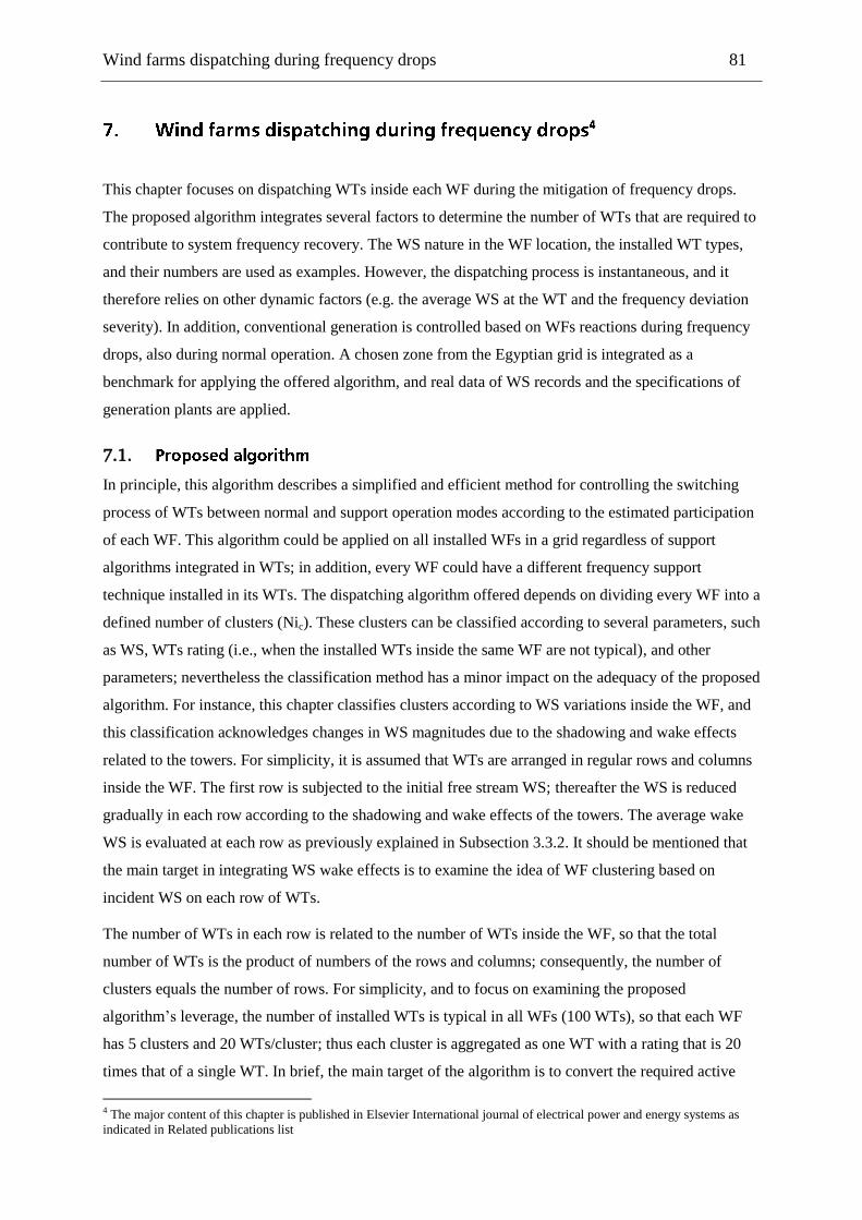
Wind farms dispatching during frequency drops 81
This chapter focuses on dispatching WTs inside each WF during the mitigation of frequency drops.
The proposed algorithm integrates several factors to determine the number of WTs that are required to
contribute to system frequency recovery. The WS nature in the WF location, the installed WT types,
and their numbers are used as examples. However, the dispatching process is instantaneous, and it
therefore relies on other dynamic factors (e.g. the average WS at the WT and the frequency deviation
severity). In addition, conventional generation is controlled based on WFs reactions during frequency
drops, also during normal operation. A chosen zone from the Egyptian grid is integrated as a
benchmark for applying the offered algorithm, and real data of WS records and the specifications of
generation plants are applied.
7.1.
In principle, this algorithm describes a simplified and efficient method for controlling the switching
process of WTs between normal and support operation modes according to the estimated participation
of each WF. This algorithm could be applied on all installed WFs in a grid regardless of support
algorithms integrated in WTs; in addition, every WF could have a different frequency support
technique installed in its WTs. The dispatching algorithm offered depends on dividing every WF into a
defined number of clusters (Nic). These clusters can be classified according to several parameters, such
as WS, WTs rating (i.e., when the installed WTs inside the same WF are not typical), and other
parameters; nevertheless the classification method has a minor impact on the adequacy of the proposed
algorithm. For instance, this chapter classifies clusters according to WS variations inside the WF, and
this classification acknowledges changes in WS magnitudes due to the shadowing and wake effects
related to the towers. For simplicity, it is assumed that WTs are arranged in regular rows and columns
inside the WF. The first row is subjected to the initial free stream WS; thereafter the WS is reduced
gradually in each row according to the shadowing and wake effects of the towers. The average wake
WS is evaluated at each row as previously explained in Subsection 3.3.2. It should be mentioned that
the main target in integrating WS wake effects is to examine the idea of WF clustering based on
incident WS on each row of WTs.
The number of WTs in each row is related to the number of WTs inside the WF, so that the total
number of WTs is the product of numbers of the rows and columns; consequently, the number of
clusters equals the number of rows. For simplicity, and to focus on examining the proposed
algorithm‘s leverage, the number of installed WTs is typical in all WFs (100 WTs), so that each WF
has 5 clusters and 20 WTs/cluster; thus each cluster is aggregated as one WT with a rating that is 20
times that of a single WT. In brief, the main target of the algorithm is to convert the required active
4 The major content of this chapter is published in Elsevier International journal of electrical power and energy systems as
indicated in Related publications list
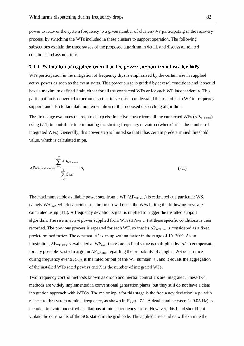
Wind farms dispatching during frequency drops 82
power to recover the system frequency to a given number of clusters/WF participating in the recovery
process, by switching the WTs included in these clusters to support operation. The following
subsections explain the three stages of the proposed algorithm in detail, and discuss all related
equations and assumptions.
WFs participation in the mitigation of frequency dips is emphasized by the certain rise in supplied
active power as soon as the event starts. This power surge is guided by several conditions and it should
have a maximum defined limit, either for all the connected WFs or for each WF independently. This
participation is converted to per unit, so that it is easier to understand the role of each WF in frequency
support, and also to facilitate implementation of the proposed dispatching algorithm.
The first stage evaluates the required step rise in active power from all the connected WFs (∆PWFs total),
using (7.1) to contribute to eliminating the stirring frequency deviation (where ‗m‘ is the number of
integrated WFs). Generally, this power step is limited so that it has certain predetermined threshold
value, which is calculated in pu.
f
WF max-
1WFs total max
WF
1
P
P s
S
X
i
iX
i
i
(7.1)
The maximum stable available power step from a WF (∆PWFi max) is estimated at a particular WS,
namely WSiavg, which is incident on the first row; hence, the WSs hitting the following rows are
calculated using (3.8). A frequency deviation signal is implied to trigger the installed support
algorithm. The rise in active power supplied from WFi (∆PWFi max) at these specific conditions is then
recorded. The previous process is repeated for each WF, so that its ∆PWFi max is considered as a fixed
predetermined factor. The constant ‗sf‘ is an up scaling factor in the range of 10–20%. As an
illustration, ∆PWFi max is evaluated at WSavg; therefore its final value is multiplied by ‗sf‘ to compensate
for any possible wasted margin in ∆PWFi max regarding the probability of a higher WS occurrence
during frequency events. SWFi is the rated output of the WF number "i", and it equals the aggregation
of the installed WTs rated powers and X is the number of integrated WFs.
Two frequency control methods known as droop and inertial controllers are integrated. These two
methods are widely implemented in conventional generation plants, but they still do not have a clear
integration approach with WTGs. The major input for this stage is the frequency deviation in pu with
respect to the system nominal frequency, as shown in Figure 7.1. A dead band between (± 0.05 Hz) is
included to avoid undesired oscillations at minor frequency drops. However, this band should not
violate the constraints of the SOs stated in the grid code. The applied case studies will examine the

Wind farms dispatching during frequency drops 83
influence of droop and inertial controller constants (KDroop, KInertia) on the performance of the proposed
algorithm.
∆PWFs total is distributed among the connected WFs so that the contribution of each WF (∆PWFi) is
calculated through (7.3); thereafter the number of participating clusters in each WF is determined
according to ∆PWFi. The weight of WF number ‗i’ (WFiweight) is a fixed parameter estimated before
running the algorithm for each WF using (7.2). In other words, WFiweight value is static and
independent from other dynamic factors such as the frequency deviation severity and WS. WFiweight is
the major parameter deciding the contribution of each WF according to the mentioned static factors
and is evaluated in (7.2) through an algebraic summation for the weights of all WFs installed in the
studied system. The implemented distribution process is based on static and dynamic factors, yet the
only dynamic factor applied in this chapter is the instantaneous approximate free stream WS
magnitude at each WF (WSi), so that the WSiinst is directly proportional to the WF contribution to
curtailment of the frequency excursion. In addition, the fixed parameters are WSiavg, installed WT
rating in WFi (WTirating), and its rated WS (WSirated). As an illustration, WSiinst is compared to the
average value of WSirated and WSiavg, as depicted in (7.3). It is of note that the final amount of ∆PWFi is
multiplied by SWFs total to convert it to MW. Thereafter this obtained value in MW is divided by SWFi to
calculate ∆PWFi in pu on the basis of the considered WFi.
Figure 7.1 Stage 1 (Droop-Inertial) controller block diagram
avg i ratingweight total weight weight
rated 1
WSi WTWFi , WFs WF
WSi
m
i
i
( 7.2)
weight . WFs totalWFi pu WF total pu
total weight avg rated WFi
WFi SP P
WFs 0.5 (WSi +WSi ) S
instWSi
(7.3)
7.1.3.
The overall contribution of a certain WF (as estimated in the previous stage) is interpreted into a
certain number of WTs that are switched to a support algorithm. However, it is difficult and

Wind farms dispatching during frequency drops 84
impractical to control each WT singularly, thus the WF is split into a certain number of clusters (Nic).
It is possible to base the clustering process on certain different approaches; one is wind-free stream
propagation inside the WF, which is used in this research work. As an illustration, the proposed
algorithm assumes a simplified relation (in particular, the number of participating clusters (Nipc) is
directly proportional to the ratio between the requested power step and the maximum allowed power
step as indicated by (7.4)).
cWFi max
NiP
WFi pu
pc
PNi
(7.4)
The obtained value for Nipc is always rounded to the lower digit, excluding values that are less than
one. As an illustration, all connected WFs have to participate in the frequency deviation mitigation;
thus, the minimum value, Nipc, during frequency events is 1. In addition, the value of Nipc is updated
every time frame (tf), which is assumed to be 5 s in this research work. Applying tf avoids unexpected
fluctuations and high transitioning rates between normal and support operation of WTs in the same
cluster. The cluster involvement priority is decided according to the incident WS at each cluster, for
instance, the first cluster facing the wind free stream has the highest priority (i.e., because WTs in this
cluster are subjected to the highest WS, hence the produced power is higher compared to that of the
WTs in other clusters). In general, the priority classification of clusters depends on the implemented
clustering theory. In relation to the three stages of the offered dispatching algorithm, the first stage is
almost identical to the conventional generation attitude during frequency drops, whereas the second
and third stages are unique to WFs and are coherently dependent on the WF‘s layout and the WTs‘
specifications, as well as WS conditions and the imposed clustering technique. To facilitate the
understanding of the proposed algorithm and to highlight its coherency and feasibility, Figure 7.2
provides a flowchart for all stages.
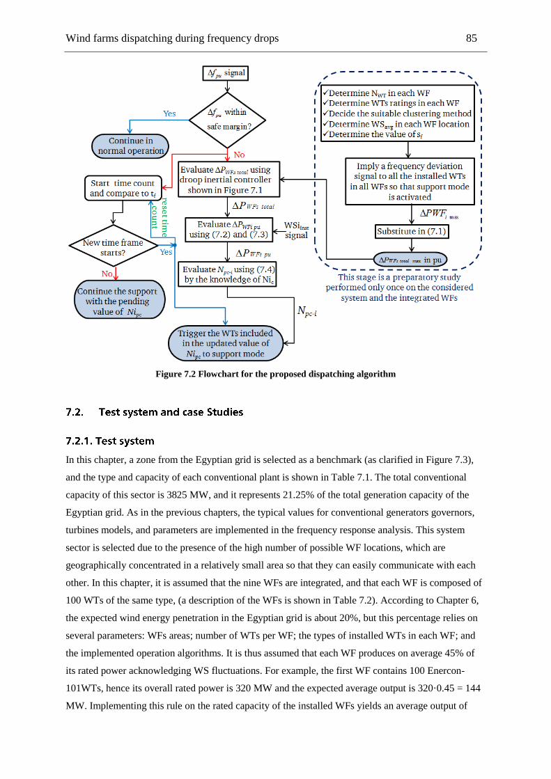
Wind farms dispatching during frequency drops 85
Figure 7.2 Flowchart for the proposed dispatching algorithm
In this chapter, a zone from the Egyptian grid is selected as a benchmark (as clarified in Figure 7.3),
and the type and capacity of each conventional plant is shown in Table 7.1. The total conventional
capacity of this sector is 3825 MW, and it represents 21.25% of the total generation capacity of the
Egyptian grid. As in the previous chapters, the typical values for conventional generators governors,
turbines models, and parameters are implemented in the frequency response analysis. This system
sector is selected due to the presence of the high number of possible WF locations, which are
geographically concentrated in a relatively small area so that they can easily communicate with each
other. In this chapter, it is assumed that the nine WFs are integrated, and that each WF is composed of
100 WTs of the same type, (a description of the WFs is shown in Table 7.2). According to Chapter 6,
the expected wind energy penetration in the Egyptian grid is about 20%, but this percentage relies on
several parameters: WFs areas; number of WTs per WF; the types of installed WTs in each WF; and
the implemented operation algorithms. It is thus assumed that each WF produces on average 45% of
its rated power acknowledging WS fluctuations. For example, the first WF contains 100 Enercon-
101WTs, hence its overall rated power is 320 MW and the expected average output is 320·0.45 = 144
MW. Implementing this rule on the rated capacity of the installed WFs yields an average output of
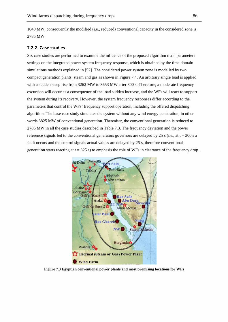
Wind farms dispatching during frequency drops 86
1040 MW, consequently the modified (i.e., reduced) conventional capacity in the considered zone is
2785 MW.
Six case studies are performed to examine the influence of the proposed algorithm main parameters
settings on the integrated power system frequency response, which is obtained by the time domain
simulations methods explained in [52]. The considered power system zone is modelled by two
compact generation plants: steam and gas as shown in Figure 7.4. An arbitrary single load is applied
with a sudden steep rise from 3262 MW to 3653 MW after 300 s. Therefore, a moderate frequency
excursion will occur as a consequence of the load sudden increase, and the WFs will react to support
the system during its recovery. However, the system frequency responses differ according to the
parameters that control the WFs‘ frequency support operation, including the offered dispatching
algorithm. The base case study simulates the system without any wind energy penetration; in other
words 3825 MW of conventional generation. Thereafter, the conventional generation is reduced to
2785 MW in all the case studies described in Table 7.3. The frequency deviation and the power
reference signals fed to the conventional generators governors are delayed by 25 s (i.e., at t = 300 s a
fault occurs and the control signals actual values are delayed by 25 s, therefore conventional
generation starts reacting at t = 325 s) to emphasis the role of WFs in clearance of the frequency drop.
Figure 7.3 Egyptian conventional power plants and most promising locations for WFs
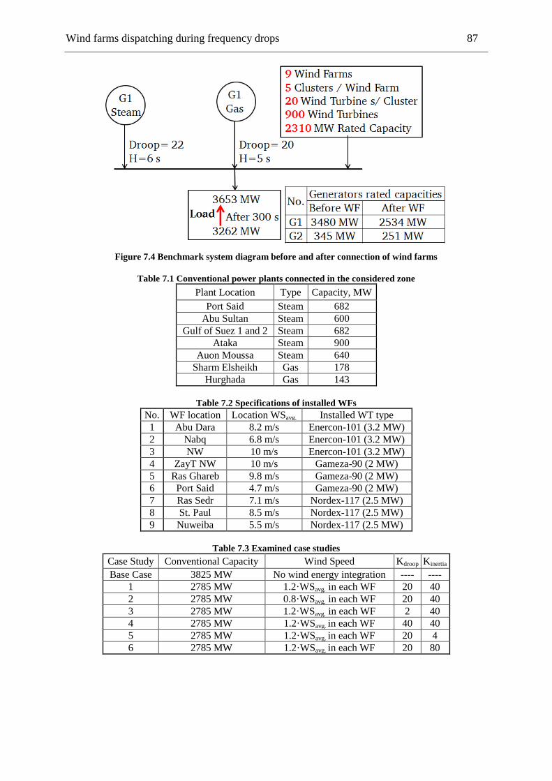
Wind farms dispatching during frequency drops 87
Figure 7.4 Benchmark system diagram before and after connection of wind farms
Table 7.1 Conventional power plants connected in the considered zone
Plant Location Type Capacity, MW
Port Said Steam 682
Abu Sultan Steam 600
Gulf of Suez 1 and 2 Steam 682
Ataka Steam 900
Auon Moussa Steam 640
Sharm Elsheikh Gas 178
Hurghada Gas 143
Table 7.2 Specifications of installed WFs
No. WF location Location WSavg. Installed WT type
1 Abu Dara 8.2 m/s Enercon-101 (3.2 MW)
2 Nabq 6.8 m/s Enercon-101 (3.2 MW)
3 NW 10 m/s Enercon-101 (3.2 MW)
4 ZayT NW 10 m/s Gameza-90 (2 MW)
5 Ras Ghareb 9.8 m/s Gameza-90 (2 MW)
6 Port Said 4.7 m/s Gameza-90 (2 MW)
7 Ras Sedr 7.1 m/s Nordex-117 (2.5 MW)
8 St. Paul 8.5 m/s Nordex-117 (2.5 MW)
9 Nuweiba 5.5 m/s Nordex-117 (2.5 MW)
Table 7.3 Examined case studies
Case Study Conventional Capacity Wind Speed Kdroop Kinertia
Base Case 3825 MW No wind energy integration ---- ----
1 2785 MW 1.2·WSavg. in each WF 20 40
2 2785 MW 0.8·WSavg. in each WF 20 40
3 2785 MW 1.2·WSavg. in each WF 2 40
4 2785 MW 1.2·WSavg. in each WF 40 40
5 2785 MW 1.2·WSavg. in each WF 20 4
6 2785 MW 1.2·WSavg. in each WF 20 80
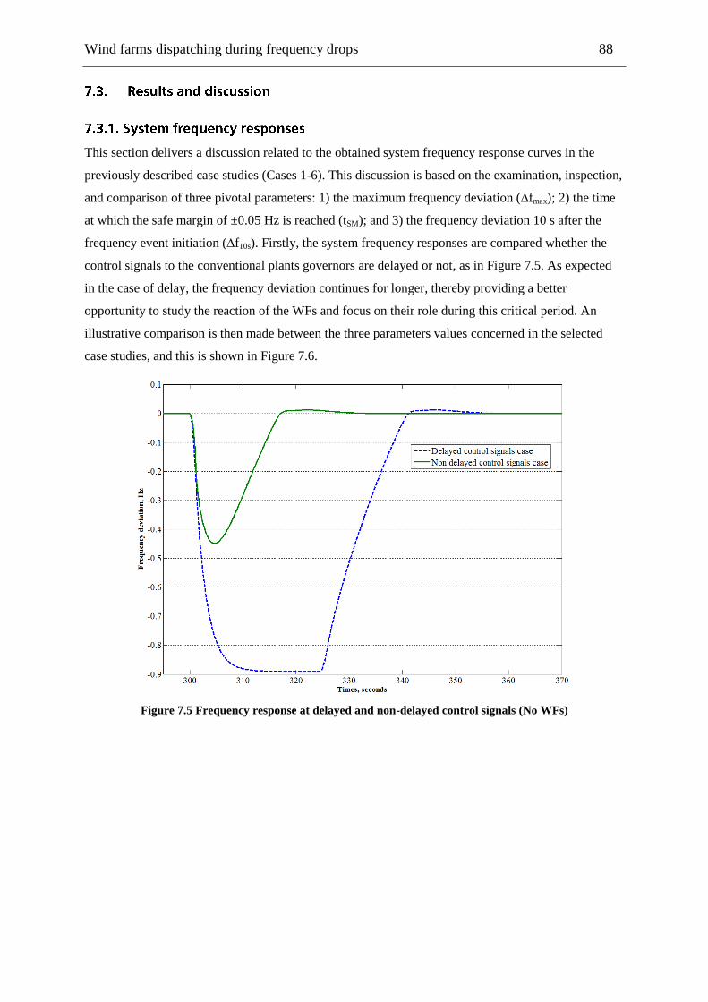
Wind farms dispatching during frequency drops 88
This section delivers a discussion related to the obtained system frequency response curves in the
previously described case studies (Cases 1-6). This discussion is based on the examination, inspection,
and comparison of three pivotal parameters: 1) the maximum frequency deviation (∆fmax); 2) the time
at which the safe margin of ±0.05 Hz is reached (tSM); and 3) the frequency deviation 10 s after the
frequency event initiation (∆f10s). Firstly, the system frequency responses are compared whether the
control signals to the conventional plants governors are delayed or not, as in Figure 7.5. As expected
in the case of delay, the frequency deviation continues for longer, thereby providing a better
opportunity to study the reaction of the WFs and focus on their role during this critical period. An
illustrative comparison is then made between the three parameters values concerned in the selected
case studies, and this is shown in Figure 7.6.
Figure 7.5 Frequency response at delayed and non-delayed control signals (No WFs)

Wind farms dispatching during frequency drops 89
Figure 7.6 Calculated parameters of frequency responses in selected cases
However, the response of Case study 2 is omitted from Figure 7.7, as it exists in a different and
inferior range of frequency deviation. Therefore, the inclusion of such a curve reduces the level of
details offered by the graph, because the frequency deviation axis range is extended. The scientific
reasons for this disparity in Case study 2 are clarified later in the relevant subsection. Most case
studies have perceptible impacts on tSM; for example, Case study 1 has the shortest tSM while Case
study 3 has the longest. An interpretation of this relies on the weak contribution of WFs in frequency
recovery when Kdroop is adjusted to a relatively low value. In particular, the low values of Kdroop and
Kinertia reduces Nipc so that the surge power injected by WFs is reduced. This is also ensured by Case
study 5, with the lowest value of Kinertia, namely, 4. In contrast, very high value of Kinertia forces the
WFs to dissipate their stored energy at an early stage and it then takes longer for them to recover to
normal operation, hence tSM is not as good, as in Case study 6. Generally, Case study 1, with average
values for Kdroop and Kinertia accompanied with a higher WS at all sites achieved the best results for tSM.
The low incident WS in all locations, namely 80% from WSavg of each site, ensured that Case study 2
was the worst. In fact, the WFs production at these WSs is not sufficient to cover the full load demand,
and certainly enough to load the conventional generators to an almost full capacity. Thus, tSM in Case
study 2 is 397 s, as most of frequency deviation elimination process is carried out by the conventional
plants. It should be highlighted that tSM in Case study 2 is removed from Figure 7.6 to focus on the
relatively smaller deficits occurring in the other cases.
The participation of WFs in the curtailment of frequency drops reduces ∆f10s, where all cases
(excluding Case study 2) have enhanced results. In particular, WFs anticipated the continuous
deterioration in frequency by providing a fast rise in active power as soon as ∆f violated the
predetermined safe margin. The best ∆f10s is achieved in Case study 5, as a result of the high values of
Kdroop and Kinertia, which amplified the amplitude of injected power surge. In spite of the poor WS
conditions in Case study 2, the injected power by the WFs mitigated ∆fmax by 0.2 Hz to within less
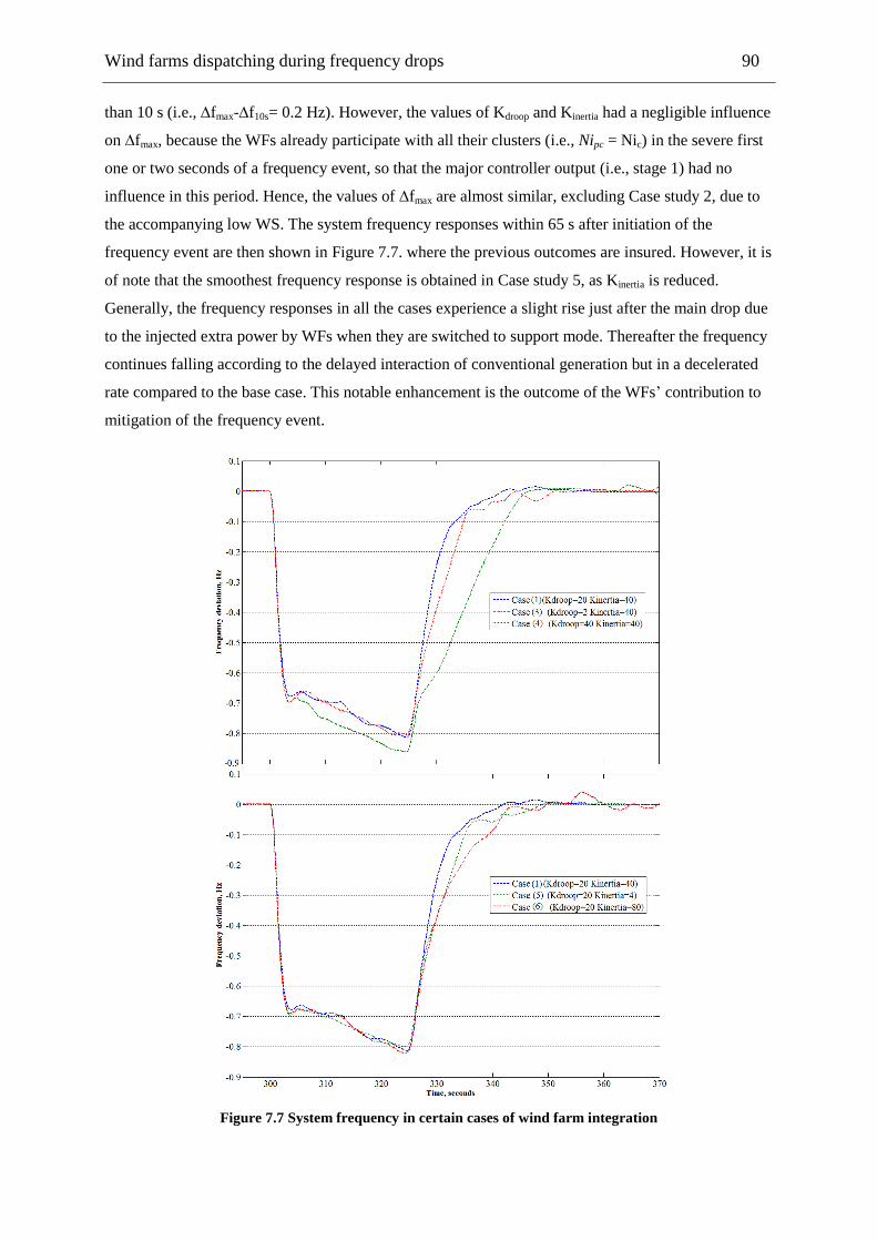
Wind farms dispatching during frequency drops 90
than 10 s (i.e., ∆fmax-∆f10s= 0.2 Hz). However, the values of Kdroop and Kinertia had a negligible influence
on ∆fmax, because the WFs already participate with all their clusters (i.e., Nipc = Nic) in the severe first
one or two seconds of a frequency event, so that the major controller output (i.e., stage 1) had no
influence in this period. Hence, the values of ∆fmax are almost similar, excluding Case study 2, due to
the accompanying low WS. The system frequency responses within 65 s after initiation of the
frequency event are then shown in Figure 7.7. where the previous outcomes are insured. However, it is
of note that the smoothest frequency response is obtained in Case study 5, as Kinertia is reduced.
Generally, the frequency responses in all the cases experience a slight rise just after the main drop due
to the injected extra power by WFs when they are switched to support mode. Thereafter the frequency
continues falling according to the delayed interaction of conventional generation but in a decelerated
rate compared to the base case. This notable enhancement is the outcome of the WFs‘ contribution to
mitigation of the frequency event.
Figure 7.7 System frequency in certain cases of wind farm integration
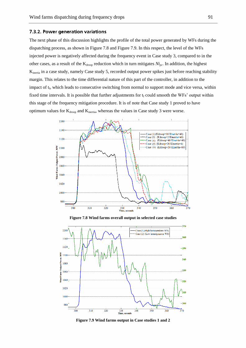
Wind farms dispatching during frequency drops 91
The next phase of this discussion highlights the profile of the total power generated by WFs during the
dispatching process, as shown in Figure 7.8 and Figure 7.9. In this respect, the level of the WFs
injected power is negatively affected during the frequency event in Case study 3, compared to in the
other cases, as a result of the Kdroop reduction which in turn mitigates Nipc. In addition, the highest
Kinertia in a case study, namely Case study 5, recorded output power spikes just before reaching stability
margin. This relates to the time differential nature of this part of the controller, in addition to the
impact of tf, which leads to consecutive switching from normal to support mode and vice versa, within
fixed time intervals. It is possible that further adjustments for tf could smooth the WFs‘ output within
this stage of the frequency mitigation procedure. It is of note that Case study 1 proved to have
optimum values for Kdroop and Kinertia, whereas the values in Case study 3 were worse.
Figure 7.8 Wind farms overall output in selected case studies
Figure 7.9 Wind farms output in Case studies 1 and 2

Wind farms dispatching during frequency drops 92
In relation to Figure 7.9, it is evident that the huge difference between the WFs‘ output power at high
and low WSs is very notable in Case studies 1 and 2, respectively. The supplied power rise in Case
study 2 is evidently limited according to insufficient wind energy. As an illustration, in Case study 1
the supplied power increases by about 140 MW within a few seconds of the frequency event, and
conversely Case study 2 records only 60 MW. Furthermore, in Case study 1, the provided power
support kept its average value constant within an acceptable period of 30 s. In contrast in Case study 2,
the low WS caused several ups and downs in the WFs output, which are spanned by short time
intervals (i.e., few seconds). These oscillations are mainly caused by the low amounts of stored KE in
WTs, and the long recovery times required by WTs to retain their default rotational speeds before they
are able to provide support again. In other words, in Case study 2, the support intervals are shortened
but the recovery durations are extended. It should be highlighted that the delay in the conventional
generation control signals ends after t=325 s, hence the required WFs support is mitigated after this
time point. Attention is also focused on conventional generation in Figure 7.10, in particular steam
generation, as it has a higher contribution. As expected, all cases are similar until t = 325 s, due to the
imposed delay in the major power and frequency control signals. However, the general process of
steam generation does not patently deviate from the base case. In other words, the base case trend is at
this point similar to the corresponding curves in other case studies, but with rescaled values due to the
WFs replacement of some conventional units, as explained in the previous section. Thus, the WFs
supplied power share in load feeding reached 28% in high WS case studies before initiation of the
frequency event. It is of note that the conventional contribution in Case study 1 is higher than that of
Case study 5. This is related to the higher Kinertia in Case study 1, so that the WFs utilize most of their
supporting capabilities within the first 25 s after initiation of the frequency event, while at the same
time the conventional reaction is retarded. In addition, Case study 5 experienced an oscillatory
response in conventional output when the frequency approaches the stability margin, because the
major controller cannot suppress ∆f fluctuations due to the low value of Kinertia. Consequently, steam
generation is reduced while the WTs are still able to provide support, or until the frequency reaches a
safe margin on one side. On the other side, steam generation increases while the WFs are recovering
their normal operational conditions.
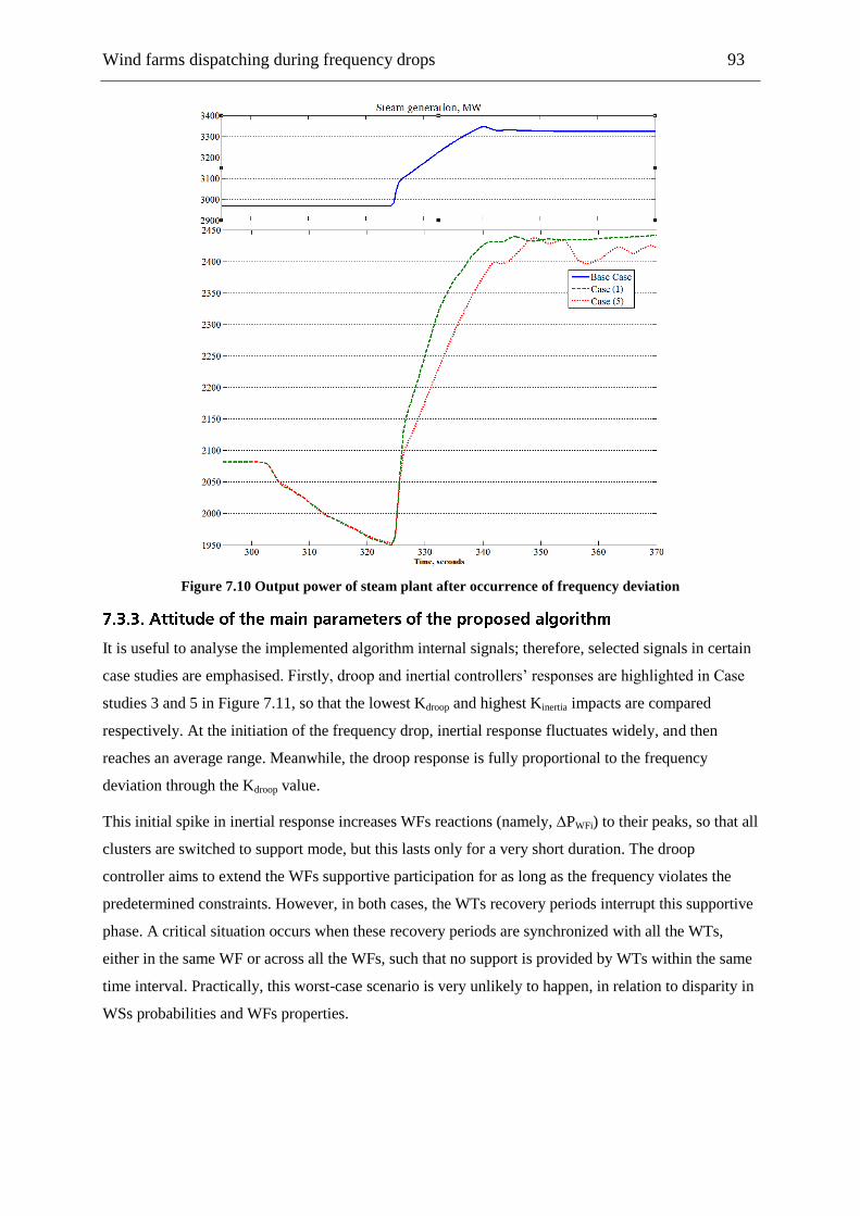
Wind farms dispatching during frequency drops 93
Figure 7.10 Output power of steam plant after occurrence of frequency deviation
It is useful to analyse the implemented algorithm internal signals; therefore, selected signals in certain
case studies are emphasised. Firstly, droop and inertial controllers‘ responses are highlighted in Case
studies 3 and 5 in Figure 7.11, so that the lowest Kdroop and highest Kinertia impacts are compared
respectively. At the initiation of the frequency drop, inertial response fluctuates widely, and then
reaches an average range. Meanwhile, the droop response is fully proportional to the frequency
deviation through the Kdroop value.
This initial spike in inertial response increases WFs reactions (namely, ∆PWFi) to their peaks, so that all
clusters are switched to support mode, but this lasts only for a very short duration. The droop
controller aims to extend the WFs supportive participation for as long as the frequency violates the
predetermined constraints. However, in both cases, the WTs recovery periods interrupt this supportive
phase. A critical situation occurs when these recovery periods are synchronized with all the WTs,
either in the same WF or across all the WFs, such that no support is provided by WTs within the same
time interval. Practically, this worst-case scenario is very unlikely to happen, in relation to disparity in
WSs probabilities and WFs properties.
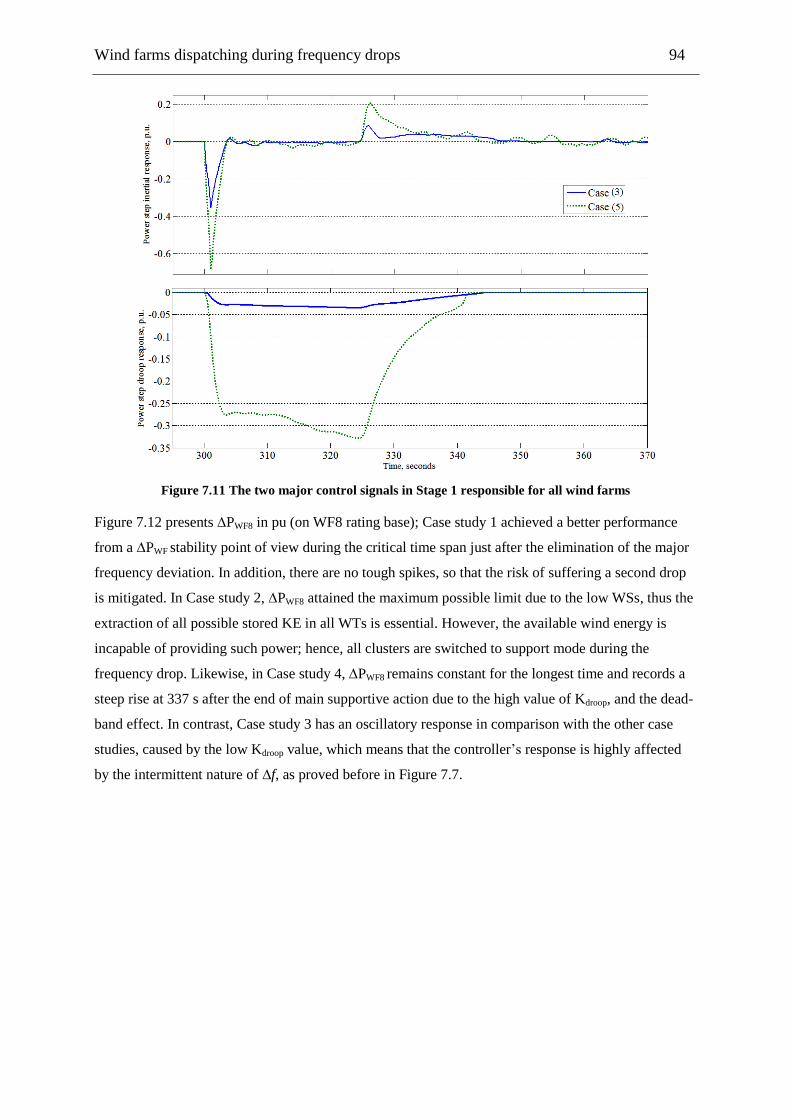
Wind farms dispatching during frequency drops 94
Figure 7.11 The two major control signals in Stage 1 responsible for all wind farms
Figure 7.12 presents ∆PWF8 in pu (on WF8 rating base); Case study 1 achieved a better performance
from a ∆PWF stability point of view during the critical time span just after the elimination of the major
frequency deviation. In addition, there are no tough spikes, so that the risk of suffering a second drop
is mitigated. In Case study 2, ∆PWF8 attained the maximum possible limit due to the low WSs, thus the
extraction of all possible stored KE in all WTs is essential. However, the available wind energy is
incapable of providing such power; hence, all clusters are switched to support mode during the
frequency drop. Likewise, in Case study 4, ∆PWF8 remains constant for the longest time and records a
steep rise at 337 s after the end of main supportive action due to the high value of Kdroop, and the dead-
band effect. In contrast, Case study 3 has an oscillatory response in comparison with the other case
studies, caused by the low Kdroop value, which means that the controller‘s response is highly affected
by the intermittent nature of ∆f, as proved before in Figure 7.7.
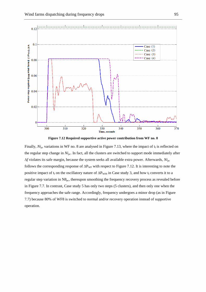
Wind farms dispatching during frequency drops 95
Figure 7.12 Required supportive active power contribution from WF no. 8
Finally, Nipc variations in WF no. 8 are analysed in Figure 7.13, where the impact of tf is reflected on
the regular step change in Nipc. In fact, all the clusters are switched to support mode immediately after
∆f violates its safe margin, because the system seeks all available extra power. Afterwards, Nipc
follows the corresponding response of ∆PWF with respect to Figure 7.12. It is interesting to note the
positive impact of tf on the oscillatory nature of ∆PWF8 in Case study 3, and how tf converts it to a
regular step variation in N8pc, thereupon smoothing the frequency recovery process as revealed before
in Figure 7.7. In contrast, Case study 5 has only two steps (5 clusters), and then only one when the
frequency approaches the safe range. Accordingly, frequency undergoes a minor drop (as in Figure
7.7) because 80% of WF8 is switched to normal and/or recovery operation instead of supportive
operation.
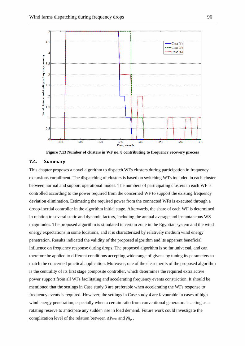
Wind farms dispatching during frequency drops 96
Figure 7.13 Number of clusters in WF no. 8 contributing to frequency recovery process
This chapter proposes a novel algorithm to dispatch WFs clusters during participation in frequency
excursions curtailment. The dispatching of clusters is based on switching WTs included in each cluster
between normal and support operational modes. The numbers of participating clusters in each WF is
controlled according to the power required from the concerned WF to support the existing frequency
deviation elimination. Estimating the required power from the connected WFs is executed through a
droop-inertial controller in the algorithm initial stage. Afterwards, the share of each WF is determined
in relation to several static and dynamic factors, including the annual average and instantaneous WS
magnitudes. The proposed algorithm is simulated in certain zone in the Egyptian system and the wind
energy expectations in some locations, and it is characterized by relatively medium wind energy
penetration. Results indicated the validity of the proposed algorithm and its apparent beneficial
influence on frequency response during drops. The proposed algorithm is so far universal, and can
therefore be applied to different conditions accepting wide range of givens by tuning its parameters to
match the concerned practical application. Moreover, one of the clear merits of the proposed algorithm
is the centrality of its first stage composite controller, which determines the required extra active
power support from all WFs facilitating and accelerating frequency events constriction. It should be
mentioned that the settings in Case study 3 are preferable when accelerating the WFs response to
frequency events is required. However, the settings in Case study 4 are favourable in cases of high
wind energy penetration, especially when a certain ratio from conventional generators is acting as a
rotating reserve to anticipate any sudden rise in load demand. Future work could investigate the
complication level of the relation between ∆PWFi and Nipc.

Storage banks for frequency support purposes 97
This chapter offers an algorithm to integrate storage battery banks in WFs to provide feasible power
support during frequency events. This algorithm determines rated powers of storage stations and
capacities according to several constraints, including WSs characteristics at the WF location. It
controls storage bank charging, discharging, and standby modes based on the acquisition of different
dynamic variables, for example WF output, load demand, and the storage cells‘ state of charge. This
algorithm is applied on a defined sector from the Egyptian grid merged with real WSs chronological
records at certain locations that are candidates to host WFs. Results reveal the positive influence of
storage banks‘ involvement on frequency excursions clearance, and in addition, wasted wind energy is
mitigated, WTs de-loading techniques are avoided, and some rejected wind power is utilized to charge
the installed storage banks. Three main topics are to be discussed: battery bank sizing,
charge/discharge control, and the expected impact on system frequency. The required storage capacity
estimation is related to probabilistic forecasting for WS at certain locations. In addition, capacity
design aim is to optimize the depth of discharge (DOD) so that battery bank life is intensively
extended [99]. The charging and discharging times are also considered to judge the required ampere-
hour capacity that allows extraction of all stored energy at a certain output power level.
Generally, storage bank (SB) sizing depends on a multi-input process compromising between
economical restrictions and technical aspects. However, this chapter concentrates on the technical side
that mitigates negative impacts of high wind energy penetration levels on frequency recovery. The
proposed algorithm acknowledges WS chronological records in a WF location, and the acceptable
level of conventional generation participation in load coverage at normal operation. In other words,
wind energy rejection is related to maintaining the participation ratio of conventional generation inside
certain boundaries, according to dynamic acquisition for load and WFs output variations. The next
steps describe using the implemented algorithm to determine the maximum possible expected charging
power and the required overall energy SB rated power and capacity:
1. WS data at a specified site are obtained in high time resolution (average WS value every 20 or 30 s),
based on the actual WSs records within the considered time span (e.g. 1 day).
2. WS arrays are incorporated with WFs models, including major details (e.g. pitch angle and
rotational speed variations) to obtain WF‘s output power arrays according to the method explained
earlier in Chapter 5. In this chapter, WS is assumed to be typical through the whole WF. Thus, the
aggregation of installed WTs equals the output of any WT multiplied by the number of WTs inside the
WF.
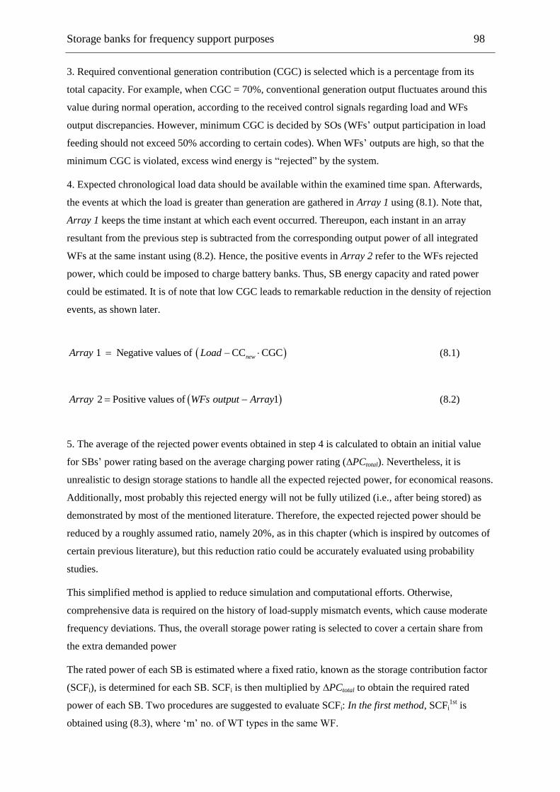
Storage banks for frequency support purposes 98
3. Required conventional generation contribution (CGC) is selected which is a percentage from its
total capacity. For example, when CGC = 70%, conventional generation output fluctuates around this
value during normal operation, according to the received control signals regarding load and WFs
output discrepancies. However, minimum CGC is decided by SOs (WFs‘ output participation in load
feeding should not exceed 50% according to certain codes). When WFs‘ outputs are high, so that the
minimum CGC is violated, excess wind energy is ―rejected‖ by the system.
4. Expected chronological load data should be available within the examined time span. Afterwards,
the events at which the load is greater than generation are gathered in Array 1 using (8.1). Note that,
Array 1 keeps the time instant at which each event occurred. Thereupon, each instant in an array
resultant from the previous step is subtracted from the corresponding output power of all integrated
WFs at the same instant using (8.2). Hence, the positive events in Array 2 refer to the WFs rejected
power, which could be imposed to charge battery banks. Thus, SB energy capacity and rated power
could be estimated. It is of note that low CGC leads to remarkable reduction in the density of rejection
events, as shown later.
1 Negative values of CC CGCnewArray Load (8.1)
2 Positive values of 1Array WFs output Array (8.2)
5. The average of the rejected power events obtained in step 4 is calculated to obtain an initial value
for SBs‘ power rating based on the average charging power rating (∆PCtotal). Nevertheless, it is
unrealistic to design storage stations to handle all the expected rejected power, for economical reasons.
Additionally, most probably this rejected energy will not be fully utilized (i.e., after being stored) as
demonstrated by most of the mentioned literature. Therefore, the expected rejected power should be
reduced by a roughly assumed ratio, namely 20%, as in this chapter (which is inspired by outcomes of
certain previous literature), but this reduction ratio could be accurately evaluated using probability
studies.
This simplified method is applied to reduce simulation and computational efforts. Otherwise,
comprehensive data is required on the history of load-supply mismatch events, which cause moderate
frequency deviations. Thus, the overall storage power rating is selected to cover a certain share from
the extra demanded power
The rated power of each SB is estimated where a fixed ratio, known as the storage contribution factor
(SCFi), is determined for each SB. SCFi is then multiplied by ∆PCtotal to obtain the required rated
power of each SB. Two procedures are suggested to evaluate SCFi: In the first method, SCFi1st
is
obtained using (8.3), where ‗m‘ no. of WT types in the same WF.

Storage banks for frequency support purposes 99
st
m*
WTi avgrated-1 1
im
1
PWT NWS /m
WSSCF
Nominator value
kk
kk
i
i
(8.3)
This formula nominator is evaluated according to the participation of each ‗WTk‘ type (i.e., the ratio
between the number and rating of each WT type with respect to other types installed in the same WF).
A resulting value is then obtained for all WTs types, taking into consideration WSavg at the WF
location. In the second method, at each time step WFi output power is divided on the overall WFs
output. Thereafter, an average value for all ratios within the considered time span is calculated
(SCF2nd
i). However, this algorithm requires enormous simulation and computational efforts when it is
applied to the whole year‘s chronological data. In this research work, it is applied only on four specific
days; the days of highest average loads in each weather season, as shown in Table 8.1. Finally, a
compromise between the two methods is applied in this using (8.4) to calculate SCFi, where ‗M‘ is the
number of SBs (i.e., WFs). This compromise is applicable as the considered time span (i.e., 4 days) is
relatively short, so that both methods are computationally feasible, and integrating the two methods
reduces the possible higher error in the first one. However, literature had also calculated storage power
ratings using other simplified methods. For example, the storage power rating is a fixed percentage of
the WF overall capacity (10 - 15% according to the results of [76, 77]).
st nd
st nd
1 2i i
i M1 2
1
SCF +SCFSCF
SCF +SCFi i
i
(8.4)
Table 8.1 Four sample days according to Egyptian grid load data
Season Winter Spring Summer Fall
24 h average load, GW 14.9 13.2 14.6 16.3
Time span (hours in year) 217-240 4273-4296 6529-6552 7561-7584
Afterwards, the number of battery cells required for each WF‘s SB is estimated based on the power
rating of the selected cell type. Consequently, the number of cells (CNi) composing each WF‘s SB is
obtained by dividing ∆PCtotal by the power rating of a single cell.
The precise location of SB inside the WF does not have deep impact on its role of supporting system
during frequency drops. However, it is more practical to construct SB warehouse near the substation
that connects the WF to the grid.
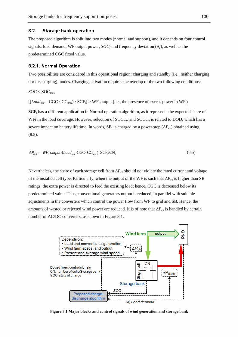
Storage banks for frequency support purposes 100
The proposed algorithm is split into two modes (normal and support), and it depends on four control
signals: load demand, WF output power, SOC, and frequency deviation (∆f), as well as the
predetermined CGC fixed value.
Two possibilities are considered in this operational region: charging and standby (i.e., neither charging
nor discharging) modes. Charging activation requires the overlap of the two following conditions:
SOC < SOCmax
[(Loadinst – CGC · CCnew) · SCFi] > WFi output (i.e., the presence of excess power in WFi)
SCFi has a different application in Normal operation algorithm, as it represents the expected share of
WFi in the load coverage. However, selection of SOCmax and SOCmin is related to DOD, which has a
severe impact on battery lifetime. In words, SBi is charged by a power step (∆Pch) obtained using
(8.5).
new i i -( -CGC CC ) SCF /CNch i i instP WF output Load (8.5)
Nevertheless, the share of each storage cell from ∆Pch should not violate the rated current and voltage
of the installed cell type. Particularly, when the output of the WF is such that ∆Pch is higher than SB
ratings, the extra power is directed to feed the existing load; hence, CGC is decreased below its
predetermined value. Thus, conventional generators output is reduced, in parallel with suitable
adjustments in the converters which control the power flow from WF to grid and SB. Hence, the
amounts of wasted or rejected wind power are reduced. It is of note that ∆Pch is handled by certain
number of AC/DC converters, as shown in Figure 8.1.
Figure 8.1 Major blocks and control signals of wind generation and storage bank

Storage banks for frequency support purposes 101
The number of integrated converters depends on the ratings and budget of available power electronics
devices. Some literature prefers a single converter for each WT, and in other approaches, one
converter is responsible for several WTs. Likewise, DC/AC converters link between SB and the power
system. For simulation simplicity, the ∆Pch is interpreted as a charging DC current fed into storage cell
model using (8.6). Moreover, minor losses and time delays of power electronics devices are ignored.
charging
ci iV CN
chPi
(8.6)
Support operation is activated when ∆f violates a predetermined limit based on grid requirement
(similar to previous chapters the safe margin is -0.05 Hz), as long as SOC > SOCmin. In support mode,
the WFs outputs are completely exploited to cover the load demand ignoring SB charging even if CGC
predetermined value is achieved. The provided power step is considered to be constant (∆Pdisch)
leading to a curtailment of the generation – demand mismatch. The value of ∆Pdisch-i is calculated using
(8.7), where Vci and Ici are the rated voltage and current of SB cell type, respectively.
disch i i i i iP =Vc Ic CN SCFtotalPC (8.7)
Most of highlighted support techniques, based on WTs stored KEs, face the risk of causing a second
frequency deviation after the depletion of extractable KE. In contrast, SBs have fixed predetermined
participation for certain defined duration (i.e., ∆Pdisch-i continues for certain support time (tSB) to reduce
the probability of second frequency excursion occurrence). tSB starts counting when ∆f reaches its
safety margin for the first time after a frequency event and it is reset when ∆f violates the safe limit.
However, tSB completion depends on SOC value such that it is prevented from violating SOCmin. tSB-i is
adjusted on a proportional basis to CNi using (8.8) to dispatch WFs‘ contributions. Thus, the switching
of all SBs from support mode to normal mode is not synchronized to mitigate the risks of successive
frequency events and incident fluctuations. For instance, the longest tSB is provided by the SB with the
highest CN (CNhighest) taking into consideration that all the cells in all SBs are typical. The tSB-longest
value is predetermined by operators (it is assumed to be 90 s so that it is relevant to the average
duration of complete clearance of moderate frequency deviations) and based on this, the tSB-i values of
other SBs are evaluated. For further illustrations, the numerical outcomes of proposed algorithm are
presented in the next section.

Storage banks for frequency support purposes 102
i
SB-i SB-longest
highest
CNt t
CN (8.8)
The test system implemented in this chapter considers a certain sector of the Egyptian 50 Hz power
system, which is the same zone implemented in Section 7.2, where nine WFs replace a certain portion
of the former conventional generation. Two types of WTs are integrated, namely, GE-77 and G-90,
and each WF includes 65 units from each type. This chapter assumes that integrated WFs actual
capacity is 50% of their rated powers, namely 1024 MW (i.e., [9 (no. of WFs) · [65 (no. of WTs from
each type) · [1.5 (rated power of GE-77) +2 (rated power of G-90))]] · 50% (assumed capacity
factor)]). Thus, the CCnew is 2801 MW (3825-1024) and the average wind power penetration is 27% of
the former conventional capacity. High resolution arrays of WSs at a 15 s time step are integrated so
that the impact of WS dynamics is acknowledged. The Egyptian grid chronological hourly load is
integrated after being de-rated by 79.9% (the ratio between the concerned sector generation capacity
and the whole grid capacity is 20.1%).
The base case study analyses the system frequency response during two successive frequency
excursions caused by a sudden rise in load demand by 8% from its actual amount (2838 MW). It then
rises steeply again after 45 s by an additional 3%.
The first and second case studies examine the frequency responses after WF integration, without
installing of SBs (Case study 1), and with SBs installed (Case study 2). The benchmark system single
line diagram, accompanied by major aspects of both implied case studies is displayed in Figure 8.2. It
is of note that the operation of the WTs in all cases is by traditional MPT, and the harvested wind
energy is fed to load or charge the SB, or is rejected according to the algorithm previously explained.
Figure 8.3 describes the variation of ∆PCtotal depending on the CGC value selection in the proposed
algorithm. ∆PCtotal escalates almost linearly with the increase of CGC. As an illustration, the rising
CGC expands the wind power rejection possibility, thus more power is available to charge the SBs.
Noticeable divergence between the four sample days relates to different WS conditions in all WFs, and
the chronological load demand. Thus, spring day results are excluded from calculating ∆PCtotal
average value, due to the very low expected rejected power on that day. However, ∆PCtotal average
value for the three days at CGC=70% is implied (i.e., ∆PCtotal = 178 MW equivalent to 4.7% from
sector capacity).
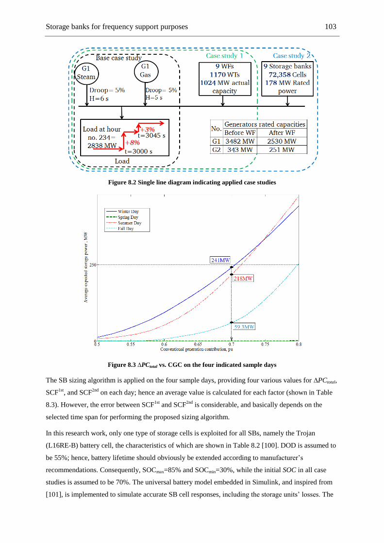
Storage banks for frequency support purposes 103
Figure 8.2 Single line diagram indicating applied case studies
Figure 8.3 ∆PCtotal vs. CGC on the four indicated sample days
The SB sizing algorithm is applied on the four sample days, providing four various values for ∆PCtotal,
SCF1st
, and SCF2nd
on each day; hence an average value is calculated for each factor (shown in Table
8.3). However, the error between SCF1st
and SCF2nd
is considerable, and basically depends on the
selected time span for performing the proposed sizing algorithm.
In this research work, only one type of storage cells is exploited for all SBs, namely the Trojan
(L16RE-B) battery cell, the characteristics of which are shown in Table 8.2 [100]. DOD is assumed to
be 55%; hence, battery lifetime should obviously be extended according to manufacturer‘s
recommendations. Consequently, SOCmax=85% and SOCmin=30%, while the initial SOC in all case
studies is assumed to be 70%. The universal battery model embedded in Simulink, and inspired from
[101], is implemented to simulate accurate SB cell responses, including the storage units‘ losses. The
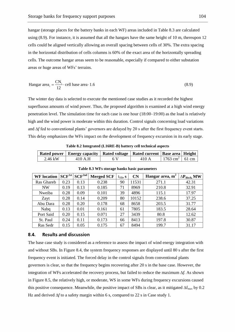
Storage banks for frequency support purposes 104
hangar (storage places for the battery banks in each WF) areas included in Table 8.3 are calculated
using (8.9). For instance, it is assumed that all the hangars have the same height of 10 m, thereupon 12
cells could be aligned vertically allowing an overall spacing between cells of 30%. The extra spacing
in the horizontal distribution of cells columns is 60% of the exact area of the horizontally spreading
cells. The outcome hangar areas seem to be reasonable, especially if compared to either substation
areas or huge areas of WFs‘ terrains.
ii
CNHangar area cell base area 1.6
12 (8.9)
The winter day data is selected to execute the mentioned case studies as it recorded the highest
superfluous amounts of wind power. Thus, the proposed algorithm is examined at a high wind energy
penetration level. The simulation time for each case is one hour (18:00–19:00) as the load is relatively
high and the wind power is moderate within this duration. Control signals concerning load variations
and ∆f fed to conventional plants‘ governors are delayed by 20 s after the first frequency event starts.
This delay emphasizes the WFs impact on the development of frequency excursion in its early stage.
Table 8.2 Integrated (L16RE-B) battery cell technical aspects
Rated power Energy capacity Rated voltage Rated current Base area Height
2.46 kW 410 A.H 6 V 410 A 1763 cm2 61 cm
Table 8.3 WFs storage banks basic parameters
WF location SCF1st
SCF2nd
Merged SCF tSB, s CN Hangar area, m2 ∆Pdisch, MW
Ras Ghareb 0.23 0.13 0.238 90 11531 271.1 42.31
NW 0.19 0.13 0.185 71 8969 210.8 32.91
Nweiba 0.28 0.09 0.101 39 4896 115.1 17.97
Zayt 0.28 0.14 0.209 80 10152 238.6 37.25
Abu Dara 0.28 0.20 0.178 68 8658 203.5 31.77
Nabq 0.13 0.01 0.161 61 7805 183.5 28.64
Port Said 0.20 0.15 0.071 27 3439 80.8 12.62
St. Paul 0.24 0.11 0.173 66 8413 197.8 30.87
Ras Sedr 0.15 0.05 0.175 67 8494 199.7 31.17
The base case study is considered as a reference to assess the impact of wind energy integration with
and without SBs. In Figure 8.4, the system frequency responses are displayed until 80 s after the first
frequency event is initiated. The forced delay in the control signals from conventional plants
governors is clear, so that the frequency begins recovering after 20 s in the base case. However, the
integration of WFs accelerated the recovery process, but failed to reduce the maximum ∆f. As shown
in Figure 8.5, the relatively high, or moderate, WS in some WFs during frequency excursions caused
this positive consequence. Meanwhile, the positive impact of SBs is clear, as it mitigated ∆fmax by 0.2
Hz and derived ∆f to a safety margin within 6 s, compared to 22 s in Case study 1.
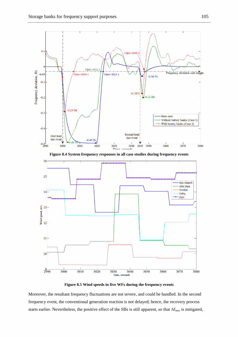
Storage banks for frequency support purposes 105
Figure 8.4 System frequency responses in all case studies during frequency events
Figure 8.5 Wind speeds in five WFs during the frequency events
Moreover, the resultant frequency fluctuations are not severe, and could be handled. In the second
frequency event, the conventional generation reaction is not delayed; hence, the recovery process
starts earlier. Nevertheless, the positive effect of the SBs is still apparent, so that ∆fmax is mitigated,
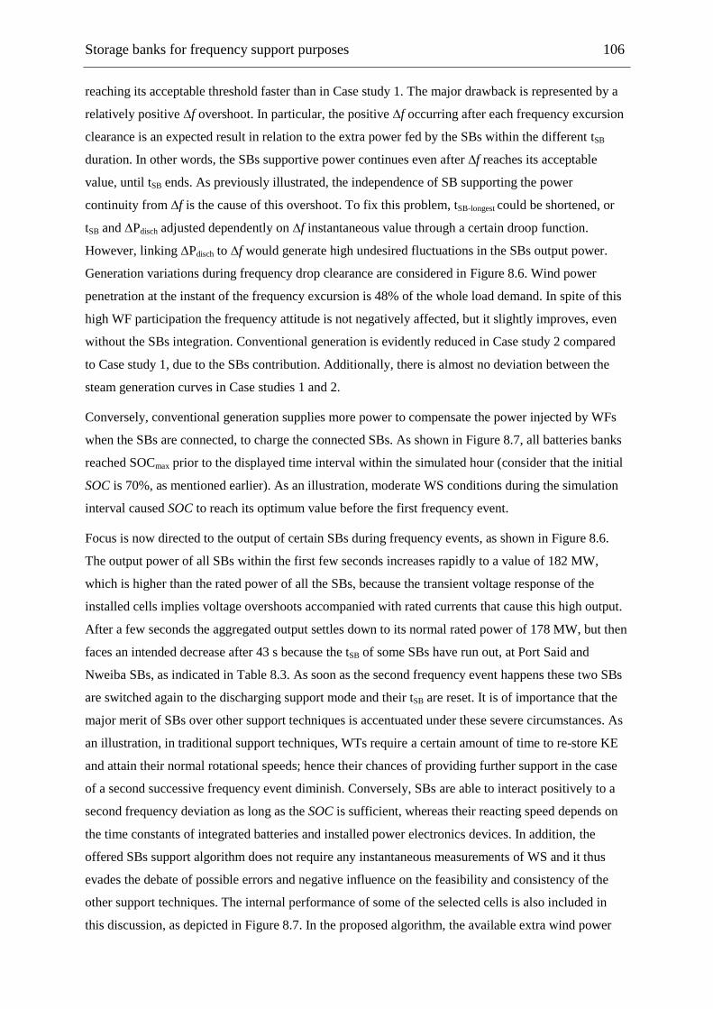
Storage banks for frequency support purposes 106
reaching its acceptable threshold faster than in Case study 1. The major drawback is represented by a
relatively positive ∆f overshoot. In particular, the positive ∆f occurring after each frequency excursion
clearance is an expected result in relation to the extra power fed by the SBs within the different tSB
duration. In other words, the SBs supportive power continues even after ∆f reaches its acceptable
value, until tSB ends. As previously illustrated, the independence of SB supporting the power
continuity from ∆f is the cause of this overshoot. To fix this problem, tSB-longest could be shortened, or
tSB and ∆Pdisch adjusted dependently on ∆f instantaneous value through a certain droop function.
However, linking ∆Pdisch to ∆f would generate high undesired fluctuations in the SBs output power.
Generation variations during frequency drop clearance are considered in Figure 8.6. Wind power
penetration at the instant of the frequency excursion is 48% of the whole load demand. In spite of this
high WF participation the frequency attitude is not negatively affected, but it slightly improves, even
without the SBs integration. Conventional generation is evidently reduced in Case study 2 compared
to Case study 1, due to the SBs contribution. Additionally, there is almost no deviation between the
steam generation curves in Case studies 1 and 2.
Conversely, conventional generation supplies more power to compensate the power injected by WFs
when the SBs are connected, to charge the connected SBs. As shown in Figure 8.7, all batteries banks
reached SOCmax prior to the displayed time interval within the simulated hour (consider that the initial
SOC is 70%, as mentioned earlier). As an illustration, moderate WS conditions during the simulation
interval caused SOC to reach its optimum value before the first frequency event.
Focus is now directed to the output of certain SBs during frequency events, as shown in Figure 8.6.
The output power of all SBs within the first few seconds increases rapidly to a value of 182 MW,
which is higher than the rated power of all the SBs, because the transient voltage response of the
installed cells implies voltage overshoots accompanied with rated currents that cause this high output.
After a few seconds the aggregated output settles down to its normal rated power of 178 MW, but then
faces an intended decrease after 43 s because the tSB of some SBs have run out, at Port Said and
Nweiba SBs, as indicated in Table 8.3. As soon as the second frequency event happens these two SBs
are switched again to the discharging support mode and their tSB are reset. It is of importance that the
major merit of SBs over other support techniques is accentuated under these severe circumstances. As
an illustration, in traditional support techniques, WTs require a certain amount of time to re-store KE
and attain their normal rotational speeds; hence their chances of providing further support in the case
of a second successive frequency event diminish. Conversely, SBs are able to interact positively to a
second frequency deviation as long as the SOC is sufficient, whereas their reacting speed depends on
the time constants of integrated batteries and installed power electronics devices. In addition, the
offered SBs support algorithm does not require any instantaneous measurements of WS and it thus
evades the debate of possible errors and negative influence on the feasibility and consistency of the
other support techniques. The internal performance of some of the selected cells is also included in
this discussion, as depicted in Figure 8.7. In the proposed algorithm, the available extra wind power

Storage banks for frequency support purposes 107
(i.e., utilized for charging of SBs) is equally distributed among the installed cells. Therefore, the SOCs
of all cells in the same SB are typical, as shown in Figure 8.7. The Nweiba SOC reaches its optimum
value after certain delay (compared to the other two SBs) due to poor WSs conditions; hence, the WF
output is barely sufficient to cover its forecasted share in load coverage, and the charging power is
restricted. At the excursion instant, all cells are discharging by the same rate as all of them are
discharging at their rated outputs. The same concept is ensured by the discharging currents' of the
three different cells.
Figure 8.6 Conventional, WFs, and storage banks output powers
Figure 8.7 Selected battery cells internal parameters performance
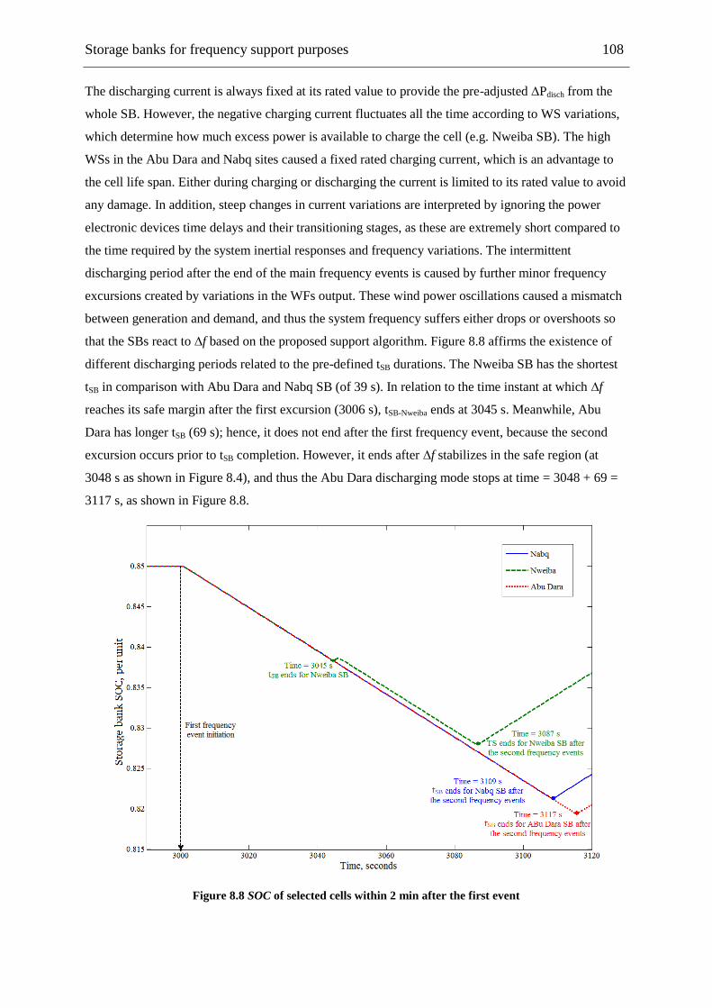
Storage banks for frequency support purposes 108
The discharging current is always fixed at its rated value to provide the pre-adjusted ∆Pdisch from the
whole SB. However, the negative charging current fluctuates all the time according to WS variations,
which determine how much excess power is available to charge the cell (e.g. Nweiba SB). The high
WSs in the Abu Dara and Nabq sites caused a fixed rated charging current, which is an advantage to
the cell life span. Either during charging or discharging the current is limited to its rated value to avoid
any damage. In addition, steep changes in current variations are interpreted by ignoring the power
electronic devices time delays and their transitioning stages, as these are extremely short compared to
the time required by the system inertial responses and frequency variations. The intermittent
discharging period after the end of the main frequency events is caused by further minor frequency
excursions created by variations in the WFs output. These wind power oscillations caused a mismatch
between generation and demand, and thus the system frequency suffers either drops or overshoots so
that the SBs react to ∆f based on the proposed support algorithm. Figure 8.8 affirms the existence of
different discharging periods related to the pre-defined tSB durations. The Nweiba SB has the shortest
tSB in comparison with Abu Dara and Nabq SB (of 39 s). In relation to the time instant at which ∆f
reaches its safe margin after the first excursion (3006 s), tSB-Nweiba ends at 3045 s. Meanwhile, Abu
Dara has longer tSB (69 s); hence, it does not end after the first frequency event, because the second
excursion occurs prior to tSB completion. However, it ends after ∆f stabilizes in the safe region (at
3048 s as shown in Figure 8.4), and thus the Abu Dara discharging mode stops at time = 3048 + 69 =
3117 s, as shown in Figure 8.8.
Figure 8.8 SOC of selected cells within 2 min after the first event

Storage banks for frequency support purposes 109
This chapter considers the impact of the integration of WFs in power systems in relation to frequency
response, particularly at frequency excursions. Battery storage banks are used to overcome any
possible drawbacks in moderate levels of wind power penetration in conventional grids. This chapter
focused on providing a feasible and detailed algorithm to estimate the power rating of the required
SBs. In addition, it offered a consistent methodology for driving the installed SB in each WF, either
during normal operating conditions or during frequency drops. Both algorithms are implemented in a
certain sector in the Egyptian grid using real WS data. A detailed analysis of frequency responses,
generation variations, and cells‘ internal parameter fluctuations are conducted. The obtained results
designate the positive influence of the applied algorithm on mitigating frequency excursions and
curtailment of the required time to reach the frequency safe margin.
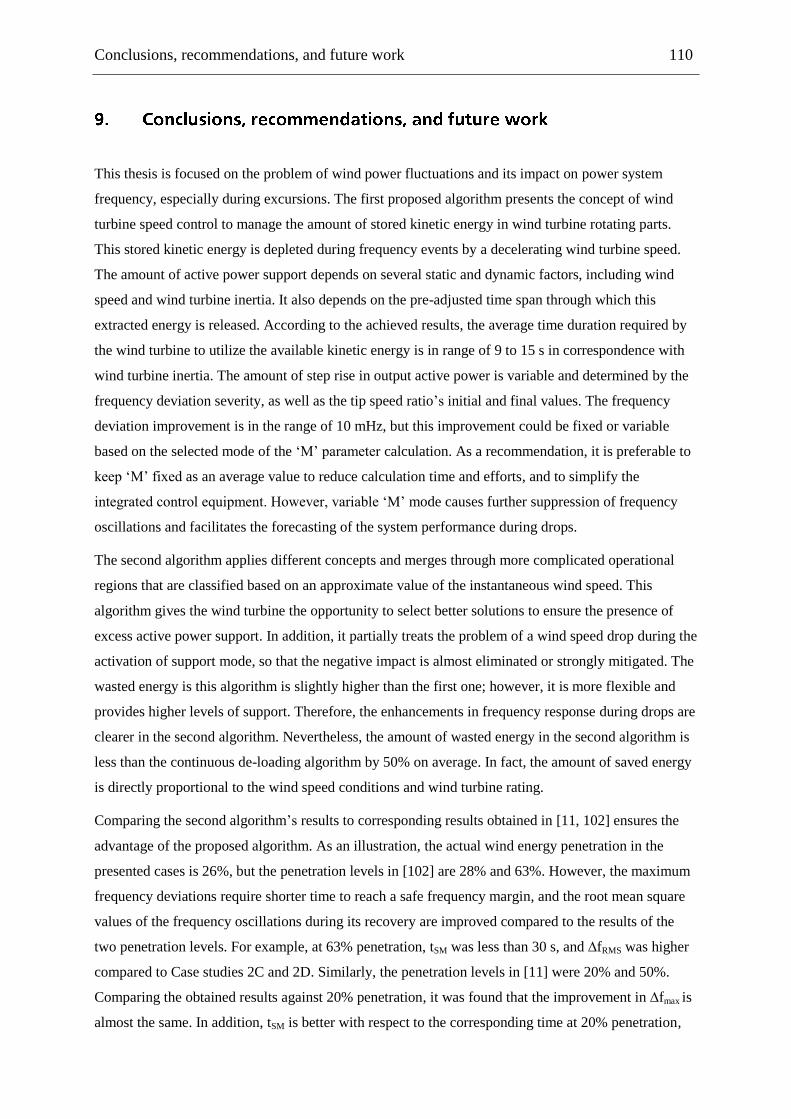
Conclusions, recommendations, and future work 110
This thesis is focused on the problem of wind power fluctuations and its impact on power system
frequency, especially during excursions. The first proposed algorithm presents the concept of wind
turbine speed control to manage the amount of stored kinetic energy in wind turbine rotating parts.
This stored kinetic energy is depleted during frequency events by a decelerating wind turbine speed.
The amount of active power support depends on several static and dynamic factors, including wind
speed and wind turbine inertia. It also depends on the pre-adjusted time span through which this
extracted energy is released. According to the achieved results, the average time duration required by
the wind turbine to utilize the available kinetic energy is in range of 9 to 15 s in correspondence with
wind turbine inertia. The amount of step rise in output active power is variable and determined by the
frequency deviation severity, as well as the tip speed ratio‘s initial and final values. The frequency
deviation improvement is in the range of 10 mHz, but this improvement could be fixed or variable
based on the selected mode of the ‗M‘ parameter calculation. As a recommendation, it is preferable to
keep ‗M‘ fixed as an average value to reduce calculation time and efforts, and to simplify the
integrated control equipment. However, variable ‗M‘ mode causes further suppression of frequency
oscillations and facilitates the forecasting of the system performance during drops.
The second algorithm applies different concepts and merges through more complicated operational
regions that are classified based on an approximate value of the instantaneous wind speed. This
algorithm gives the wind turbine the opportunity to select better solutions to ensure the presence of
excess active power support. In addition, it partially treats the problem of a wind speed drop during the
activation of support mode, so that the negative impact is almost eliminated or strongly mitigated. The
wasted energy is this algorithm is slightly higher than the first one; however, it is more flexible and
provides higher levels of support. Therefore, the enhancements in frequency response during drops are
clearer in the second algorithm. Nevertheless, the amount of wasted energy in the second algorithm is
less than the continuous de-loading algorithm by 50% on average. In fact, the amount of saved energy
is directly proportional to the wind speed conditions and wind turbine rating.
Comparing the second algorithm‘s results to corresponding results obtained in [11, 102] ensures the
advantage of the proposed algorithm. As an illustration, the actual wind energy penetration in the
presented cases is 26%, but the penetration levels in [102] are 28% and 63%. However, the maximum
frequency deviations require shorter time to reach a safe frequency margin, and the root mean square
values of the frequency oscillations during its recovery are improved compared to the results of the
two penetration levels. For example, at 63% penetration, tSM was less than 30 s, and ∆fRMS was higher
compared to Case studies 2C and 2D. Similarly, the penetration levels in [11] were 20% and 50%.
Comparing the obtained results against 20% penetration, it was found that the improvement in ∆fmax is
almost the same. In addition, tSM is better with respect to the corresponding time at 20% penetration,

Conclusions, recommendations, and future work 111
and almost equivalent at 50%. As a recommendation, the second algorithm is preferred for wind
turbines equipped with pitch controllers and at high levels of wind energy penetration. In addition, it is
more efficient for wind farms locations that are characterized by low average wind speeds. It is of note
that overloading the wind turbine generator proved to be a feasible solution at high wind speeds,
because it avoids de-loading at these wind speeds, and hence reduces wasted energy. The dispatching
algorithm has improved this method and, and has proved to be an essential part in completing the
support process and reducing frequency oscillations. The major inertial droop controller (which
manages the number of participating clusters in frequency support) makes the wind farm operation
equivalent to conventional generation; however, it slightly mitigates the achievement improvements in
frequency recovery. In other words, integrating the second algorithm with the proposed dispatching
method provides a reasonable solution for enabling wind farms to contribute positively in the
elimination of frequency drops.
This thesis also presents a modified method of estimating a round figure for the upgraded conventional
capacity after certain wind farms integration. This method mainly relies on the amount of annual
generated energy by a certain wind turbine type according to wind speed chronological data in a
concerned location. Results show that the annual energy generation ranges from 35% up to 73% (in
very limited locations) of continuous full load generation. Examined locations and wind turbine types
reveal that large wind turbines with a wide range of rotational speeds are the best choice for moderate
or low wind speed sites. However, medium-sized cheaper wind turbines are acceptable in locations
with high average wind speeds. According to the Egyptian case study capacity assessment, thirteen
wind farms with 1300 wind turbines from three different manufacturers can replace 20% of
conventional generation without the need to use reserves. These numbers are obtained using tough
constraints, as the energy production analysis was performed using the top 10% of records of the
Egyptian grid‘s hourly load. However, this number is a round figure, which is highly affected by the
matching criterion between wind turbines types and integrated locations. In addition, the worst
frequency deviation occurred due to this replacement at standard operation for wind turbines, did not
exceed 40 mHz during the hour of peak load record.
The integration of storage banks as an alternative source of power support has also proved to be valid.
In particular, the construction of a batteries hangar near the connection point of each wind farm is a
practical solution, and it avoids any ‗special‘ algorithm for wind turbine operation. The achieved
frequency improvement is almost similar to enhancements achieved in the first and second algorithms,
but with better sustainability. In addition, wasted wind energy is reduced to zero in this case but more
wind energy is utilized when the batteries are charged. However, the criterion used to decide whether
excess wind energy is available to charge the batteries banks is a point of further investigations. In this
research work, it is assumed that the conventional generation contribution in the load feed should be in
the range of 70% of the total demand, and that the remaining 30% would be covered by wind farms. If
the generation from wind farms is higher than the required power to fulfil this requirement, the excess

Conclusions, recommendations, and future work 112
energy is directed to charge the battery banks. In relation to the applied case study, it is evident that
storage banks with an overall rated power of 8.7% (from the nameplate ratings of installed wind
farms) clearly improve the frequency response during drops. In general, there are markedly improved
achievements in frequency, because maximum drop is alleviated by 150 mHz, with a reduction of 10 s
in reaching the safety margin. In addition, it was found that reducing the average participation of
conventional generation in the load feed will dramatically reduce the power rating of the required
storage banks.
It is possible that future work will investigate the integration of a central pumped-hydro storage
facility as an alternative to all battery banks. The presence of several water resources in Egypt, and the
suitable geographical nature in some areas, makes it feasible to construct hydro energy storage
reservoirs. Thus, the excess wind power could be used to lift the water from the natural resource to a
higher level, and the available hydro power could be utilized either for support in frequency events, or
to mitigate the intermittent nature of wind power generation. In addition, future work will highlight
reliability studies to calculate load interruptions indices at major load points after the replacement of
conventional units. The real reliability data of both conventional units and wind turbines will be
involved, as well as the precise distribution of economic load categories. It is also possible that the
economic impacts of the proposed support algorithms could be examined and compared to a standard
maximum power tracking operation and its economical merits. Likewise, the capital and running costs
of integrating possible storage mediums would be estimated and compared with the extra financial
burdens that will occur due to implementation of the proposed frequency support algorithms.

Bibliography 113
[1] T. Hartkopf, Lecture notes - Renewable energies. Darmstadt: Technical University of
Darmstadt, 2010.
[2] R. Thresher, M. Robinson, and P. Veers, "To capture the wind," IEEE power energy Magazine,
vol. 5, no. 6, 2007.
[3] Z. Xu, M. Gordon, M. Lind, and J. Ostergaard, "Towards a danish power system with 50% wind
— smart grids activities in Denmark," in IEEE Power & Energy Society General Meeting,
Lyngby, 2009.
[4] T. Ackermann, Wind power in power systems. John Wiley & Sons Ltd, 2005.
[5] T. Burton, D. Sharpe, N. Jenkins, and E. Bossanyi, Wind energy handbook. John Wiley & Sons
Ltd, 2001.
[6] B. Fox, L. Bryans, D. Flynn, N. Jenckins, and D. Milborrow, Wind power integration. IET
Power and Energy Series 50, 2007.
[7] G. Michalke, PhD thesis-Variable speed wind turbines - modeling, control, and impact on
power system. Darmstadt: Darmstadt University of technology, 2008.
[8] S. Engelhardt, I. Erlich, C. Feltes, J. Kretschmann, and F. Shewarega, "Reactive power
capability of wind turbines based on doubly fed induction generators," IEEE Transactions on
Energy Conversion, vol. 26, no. 1, pp. 364-372, 2011.
[9] R. Doherty, et al., "An assessment of the impact of wind generation on system frequency
control," IEEE Transactions on Power Systems, vol. 25, no. 1, pp. 452-460, 2010.
[10] A. R. Bergen and V. Vittal, Power system analysis, Second edition. Prentice Hall, 2000.
[11] L.-R. Chang-Chien, C.-M. Hung, and Y.-C. Yin, "Dynamic reserve allocation for system
contingency by DFIG wind farms," IEEE transactions on Power Systems, vol. 23, no. 2, pp.
729-736, 2008.
[12] V. Akhmatov, PhD Thesis- Analysis of dynamic behaviour of electrical power systems with
large amounts of wind energy. Lyngby: Technical University of Denmark, 2003.
[13] M. Tazil, et al., "Three-phase doubly fed induction generators: an overview," IET Journal of
Electric Power Applications, vol. 4, no. 2, pp. 75-89, 2009.
[14] H. Polinder, S. W. H. De Haan, M. R. Dubois, and J. G. Slootweg, "Basic operation principles
and electrical conversion systems of wind turbines," European power electronics and drives
journal, vol. 15, no. 4, 2005.
[15] L. Y. Pao and K. E. Johnson, "Control of wind turbines," IEEE Control System magazine, vol.
31, no. 2, pp. 44-62, 2011.
[16] A. Perdana, PhD thesis-Dynamic model of wind turbines, a contribution towards the
establishment of standardized models of wind turbines for power system stability studies.
Sweden: Chalmers university of technology, 2008.
[17] N. Miller, W. Price, and J. Sanchez-Gasca, "Dynamic modeling of GE 1.5 and 3.6 wind turbine-
generators," in Power Engineering Society General Meeting, New York, 2003.
[18] A. B. Attya and T. Hartkopf, "Evaluation of wind turbines dynamic model parameters using
published manufacturer product data," in IEEE International Energy Conference and Exhibition,
Florence, 2012.
[19] Y. Zou, M. Elbuluk, and Y. Sozer, "A complete modeling and simulation of induction generator
wind power systems," in IEEE Industry Applications Society Annual Meeting, Houston, 2010.
[20] A. Grauers, "Efficiency of three wind energy generator systems," IEEE Transactions on Energy
Conversion, vol. 11, no. 3, pp. 650-657, 1996.
[21] Enercon company, (2011) Enercon wind turbines - product overview. [Online].
http://www.enercon.de/p/downloads/ENERCON_PU_en.pdf
[22] U. S. department of energy, (2012) Documentation, user support, and verification of wind
turbine and plant models. [Online]. http://www.osti.gov/bridge/servlets/purl/1051403/.pdf

Bibliography 114
[23] S. Nishikata and F. Tatsuta, "A new interconnecting method for wind turbine generators in a
wind Farm and basic performances of the integrated system," IEEE Transactions on Industrial
Electronics, vol. 57, no. 2, pp. 468-475, 2010.
[24] M. Jelavić, N. Perić, and I. Petrović, "Damping of wind turbine tower oscillations through rotor
speed control," in International Conference on Ecologic Vehicles & Renewable Energies,
Monaco, 2007.
[25] M. Qian, N. Chen, L. Zhao, D. Zhao, and L. Zhu, "A new pitch control strategy for variable-
speed wind generator," in IEEE Innovative Smart Grid Technologies - Asia, Tianjin, 2012.
[26] T. Senjyu, et al., "Output power control of wind turbine generator by pitch angle control using
minimum variance control," Wiley library- Electrical engineering in Japan, vol. 154, no. 2, pp.
10-18.
[27] I. A. Hiskens, "Dynamics of type-3 wind turbine generator models," IEEE Transactions on
Power Systems, vol. 27, no. 1, pp. 465-474, 2012.
[28] L. Yang, Z. Xu, J. Ostergaard, Z. Y. Dong, and K. P. Wong, "Advanced control strategy of
DFIG wind turbines for power system fault ride through," IEEE Transactions on Power
Systems, vol. 27, no. 2, pp. 713-722, 2012.
[29] S.-B. Lee and K.-B. Lee, "Performance improvement of a DFIG in a wind turbine under an
unbalanced grid-voltage condition," in IEEE International Symposium on Industrial Electronics,
Italy, 2010.
[30] J. Hu and Y. He, "Reinforced control and operation of DFIG-based wind power generation
system under unbalanced grid voltage conditions," IEEE Transactions on Energy Conversion,
vol. 24, no. 4, pp. 905-915, 2009.
[31] D. Xiang, L. Ran, J. R. Bumby, P. J. Tavner, and S. Yang, "Coordinated control of an HVDC
link and doubly fed induction generators in a large offshore wind farm," IEEE Transactions on
Power Delivery, vol. 21, no. 1, pp. 463-471, 2006.
[32] J. F. M. Padron and A. E. F. Lorenzo, "Calculating steady-state operating conditions for doubly-
fed induction generator wind turbines," IEEE Transactions on Power Systems, vol. 25, no. 2, pp.
922-928, 2010.
[33] Z. J. Meng, "An improved equivalent wind method for the aggregation of DFIG wind turbines,"
in IEEE International Conference on Power System Technology, China, 2010.
[34] S. Li, T. A. Haskew, and S. Mazari, "Integrating electrical and aerodynamic characteristics for
DFIG speed control study," in IEEE Power Systems Conference and Exposition, Seattle, 2009.
[35] S. M. Muyeen, et al., "Low voltage ride through capability enhancement of wind turbine
generator system during network disturbance," IET Renewable Power Generation, vol. 3, no. 1,
pp. 65-74, 2009.
[36] O. Aluko, T. M. Smith, and L. M. Tolbert, "Behavior of doubly-fed induction generator under
nearby wind plant fault," in IEEE Power and Energy Society General Meeting, Tennessee, USA,
2010.
[37] N. Joshi and N. Mohan, "A novel scheme to connect wind turbines to the power grid," IEEE
Transactions on Energy Conversion, vol. 24, no. 2, pp. 504-510, 2009.
[38] J. Hu, et al., "A novel control strategy for doubly fed induction generator and permanent magnet
synchronous generator during voltage dips," in 20th Australasian Universities Power
Engineering Conference, Australia, 2010.
[39] A. D. Hansen and G. Michalke, "Fault ride-through capability of DFIG wind turbines," Elsevier
Renewable Energy, vol. 32, no. 9, p. 1594–1610, 2006.
[40] L. Peng, B. Francois, and Y. Li, "Improved crowbar control strategy of DFIG based wind
turbines for grid fault ride-through," in IEEE 24th Applied Power Electronics Conference and
Exposition, Washington, DC, 2009, pp. 1932-1938.
[41] G. Pannell, D. J. Atkinson, and B. Zahawi, "Minimum-threshold crowbar for a fault-ride-
through grid-code-compliant DFIG wind turbine," IEEE Transactions on Energy Conversion,
vol. 25, no. 3, pp. 750-759, 2010.

Bibliography 115
[42] R. G. de Almeida and J. A. Peas Lopes, "Participation of doubly fed induction wind generators
in system frequency regulation," IEEE Transactions on Power Systems, vol. 22, no. 3, pp. 944-
950, 2007.
[43] H. Holttinen, et al., "Currents of changes," IEEE Power and Energy Magazine, vol. 9, no. 6, pp.
47-59, 2011.
[44] I. R. Unknown, "Dynamic models for steam and hydro turbines in power system studies," IEEE
Transactions on Power Apparatus System, vol. 92, no. 6, pp. 1904-1915, 1973.
[45] M. Bhuiyan and S. Dinakar, Master thesis-Comparing and evaluating frequency response
characteristics of conventional power plant with wind power plant. Goteborg: Chalmers
University of Technology, 2008.
[46] O. Anaya-Lara, F. M. Hughes, N. Jenkins, and G. Strbac, "Contribution of DFIG-based wind
farms to power system short-term frequency regulation," in IEE Proceedings- Generation,
Transmission and Distribution, Manchester, 2006.
[47] J. Ekanayake and N. Jenkins, "Comparison of the response of doubly fed and fixed-speed
induction generator wind turbines to changes in network frequency," IEEE Transactions on
Energy Conversion, vol. 19, no. 4, pp. 802-812, 2004.
[48] J. Berdy. (2010) Out-of-step protection for generators. [Online].
http://store.gedigitalenergy.com/FAQ/Documents/CEB/GER-3179.pdf
[49] N. Rahmat Ullah, T. Thiringer, and D. Karlsson, "Temporary primary frequency control support
by variable speed wind turbines - potenial and applications," IEEE Transactions on Power
Systems, vol. 23, no. 2, pp. 601-612, 2008.
[50] M. F. M. Arani and E. F. El-Saadany, "Implementing virtual inertia in DFIG-based wind power
generation," IEEE Transactions on Power Systems, vol. 28, no. 2, pp. 1373-1384, 2012.
[51] D. L. Yao, S. S. Choi, K. J. Tseng, and T. T. Lie, "Determination of short-term power dispatch
schedule for a wind farm incorporated with dual-battery energy storage scheme," IEEE
Transactions on Sustainable Energy, vol. 3, no. 1, pp. 74-84, 2012.
[52] P. Kundur, Power system stability and control. 1994: McGraw-Hill Inc., New York.
[53] G. Andersson, Lecture notes: Dynamics and control of eletrical power systems. Zurich: ETH
Zurich, 2011.
[54] S. Muller, M. Deicke, and W. D. Doncker, "Double fed induction generator for wind turbine
systems," IEEE Industry Applications Magazine, vol. 8, no. 3, pp. 26-33, 2002.
[55] W. Leonhard, Control of electrical drives, 3rd ed. Springer , 2001.
[56] T. R. Ayodele, A. A. Jimoh, J. L. Munda, and J. T. Agee, "Impact of variation of wind speed in
a wind integrated power system," in International Conference on Advances in Energy
Engineering (ICAEE), Tshwane, South Africa, 2010.
[57] S.-J. Huang and H.-H. Wan, "Enhancement of matching turbine generators with wind regime
using capacity factor curves strategy," IEEE Transactions on Energy Conversion, vol. 24, no. 2,
pp. 551-553, 2009.
[58] A. Kusiak and Z. Zhang, "Short-horizon prediction of wind power: A data-driven approach,"
IEEE Transactions on Energy Conversion, vol. 25, no. 4, pp. 1112-1122, 2010.
[59] A. Kusiak, H. Zheng, and Z. Song, "Short-term prediction of wind farm power: a data mining
approach," IEEE Transactions on Energy Conversion, vol. 24, no. 1, pp. 125-136, 2009.
[60] M. Narayana, G. Putrus, M. Jovanovic, and P. S. Leung, "Predictive control of wind turbines by
considering wind speed forecasting techniques ," in 44th International Universities Power
Engineering Conference, Glasgow, 2009 .
[61] P. Clemow, T. C. Green, and C. A. Hernandez-Aramburo, "Wind farm output smoothing
through co-ordinated control and short-term wind speed prediction," in IEEE Power and Energy
Society General Meeting, London, 2010.
[62] R. J. Barthelmie and L. E. Jensen, "Evaluation of wind farm efficiency and wind turbine wakes
at the nysted offshore wind farm," Willey wind energy journal, vol. 13, no. 6, p. 573–586, 2010.
[63] M. Magnusson and A. .-S. Smedman, "Air flow behind wind turbines," Wind Engineering and

Bibliography 116
Industrial Aerodynamics, vol. 80, no. 1-2, pp. 169-189, 1999.
[64] L. M. Frenandez, C. A. Garcia, J. R. Saenz, and F. Jurado, "Equivalent models of wind farms by
using aggregated wind turbines and equivalent winds," Elsevier Journal of Energy Conversion
and Management, vol. 50, no. 3, pp. 691-704, 2009.
[65] M. Ali, I. .-S. Ilie, J. V. Milanovic, and G. Chicco, "Wind farm model aggregation using
probabilistic clustering," IEEE Transactions on Power Systems, vol. 28, no. 1, pp. 309-316,
2012.
[66] B. P. Hayes, I. Ilie, A. Porpodas, S. Z. Djokic, and G. Chicco, "Equivalent power curve model of
a wind farm based on field measurement data," in IEEE PowerTech, Trondheim, 2011.
[67] M. Ali, J. Matevosyan, J. V. Milanović, and L. Söder, "Effect of wake consideration on
estimated cost of wind energy curtailments," in 8th Int. Workshop Large-Scale Integration of
Wind Power into Power Systems and on Transmission Networks for Offshore Wind Farms,
Bremen, 2009.
[68] J. Ekanayake, K. Liyanage, J. Wu, A. Yokoyama, and N. Jenkins, Smart grid: technology and
applications. New Delhi, India.: John Wiley & Sons, 2012.
[69] X. Liu and W. Xu, "Economic load dispatch constrained by wind power availability: A here-
and-now approach," IEEE Transactions on Sustainable Energy, vol. 1, no. 1, pp. 2-9, 2010.
[70] L. Li, Q. Ding, H. Li, and M. Dan, " Optimal dispatching method for smoothing power
fluctuations of the wind-photovoltaic-battery hybrid generation system ," in IEEE Asia
Innovative Smart Grid Technologies, Tianjin, 2012.
[71] A. B. Attya and T. Hartkopf, "Penetration impact of wind farms equipped with frequency
variations ride through algorithm on power system frequency response," International Journal
of Electrical Power and Energy Systems, vol. 40, no. 1, pp. 94-103, 2012.
[72] J. A. Martinez, "Modeling and characterization of energy storage devices," in IEEE Power and
Energy Society general meeting, San Diego, 2011.
[73] T. K. A. Brekken, et al., "Optimal energy storage sizing and control for wind power
applications," IEEE Transactions on Sustainable Energy, vol. 2, no. 1, pp. 69-77, 2011.
[74] B. Hartmann and A. Dan, "Cooperation of a grid-connected wind farm and an energy storage
unit — demonstration of a simulation tool," IEEE Transactions on Sustainable Energy, vol. 3,
no. 1, pp. 49-56, 2012.
[75] S. Teleke, M. E. Baran, A. Q. Huang, S. Bhattacharya, and L. Anderson, "Control strategies for
battery energy storage for wind farm dispatching," IEEE Transactions on Sustainable Energy,
vol. 3, no. 2009, pp. 725-732, 2009.
[76] S. Teleke, M. E. Baran, A. Q. Huang, and S. Bhattacharya, "Rule-based control of battery
energy storage for dispatching intermittent renewable sources," IEEE Transactions on
Sustainable Energy, vol. 1, no. 3, pp. 117-124, 2010.
[77] D. L. Yao, S. S. Choi, K. J. Tseng, and T. T. Lie, "A statistical approach to the design of a
dispatchable wind power-battery energy storage system," IEEE Transactions on Energy
Conversion, vol. 24, no. 4, pp. 916-925, 2009.
[78] D. Gautam, V. Vittal, and T. Harbour, "Impact of increased penetration of DFIG-based wind
turbine generators on transient and small signal stability of power systems," IEEE transactions
on Power Systems, vol. 24, no. 3, pp. 1426-1434, 2009.
[79] C.-C. Le-Ren and Y. Yao-Ching, "Strategies for operating wind power in a similar manner of
conventional power plant," IEEE transactions on energy conversion, vol. 24, no. 4, pp. 926-934,
2009.
[80] P.-K. Keung, L. Pei, H. Banakar, and O. Boon Teck, "Kinetic energy of wind-turbine generators
for system frequency support," IEEE transactions on Power Systems, vol. 24, no. 1, pp. 279-
287, 2009.
[81] G. C. Tarnowski, P. C. Kjar, P. E. Sorensen, and J. Ostergaard, "Variable speed wind turbines
capability for temporary over-production," in Proceedings of IEEE Power & Energy Society
General Meeting, USA, 2009.

Bibliography 117
[82] M. Kayikci and J. V. Milanovic, "Dynamic contribution of DFIG-based wind plants to system
frequency disturbances," IEEE transactions on Power Systems, vol. 24, no. 2, pp. 859-867,
2009.
[83] I. W. G. R. Unknown, "Hydraulic turbine and turbine control models for system dynamic
studies," IEEE Transactions on Power Systems, vol. 7, no. 1, pp. 167-179, 1992.
[84] H. Emam Shalan, M. A. Moustafa Hassan, and A. B. G. Bahgat, "Parameter estimation and
dynamic simulation of gas turbine model in combined cycle power plants based on actual
operational data," Journal of American Science, vol. 7, no. 5, pp. 303-310, 2011.
[85] N. Jaleeli, D. N. Ewart, and L. H. Fink, "Understanding automatic generation control," IEEE
Transactions on Power Systems, vol. 7, no. 3, pp. 1106-1122, 1992.
[86] A. B. Attya, Y. G. Hegazy, and M. A. Mostafa, "Evaluation of system reliability using seasonal
and random operation techniques," in IEEE Power Engineering Society General Meeting,
Pittsburgh, 2008.
[87] A. B. Attya and T. Hartkopf, "Generation of High Resolution Wind Speeds and Wind Speed
Arrays inside a Wind Farm based on Real Site Data," in IEEE 11th conference on electrical
power quality and utilization, Lisbon, 2011.
[88] N. Moskalenko, K. Rudion, and A. Orths, "Study of wake effects for offshore wind farm," in
Modern Electric Power Systems, Wroclaw, Poland, 2010.
[89] P. Frohboese and C. Schmuck, "Thrust coefficients used for estimation of wake effects of
fatigue load calculation," in Proceedings of European Wind Energy Conference, Warsaw,
Poland, 2010.
[90] A. Keane, et al., "Capacity value of wind power," IEEE Transactions on Power Systems, vol. 26,
no. 2, pp. 564-572, 2011.
[91] I. A. Gowaid, A. El-Zawawi, and M. El-Gammal, "Improved inertia and frequency support from
grid-connected DFIG wind farms," in IEEE Power Systems Conference and Exposition, USA,
2011.
[92] M. Faridi, R. Ansari, S. A. Mousavi, and M. Dodman, "Pitch control of wind turbine blades in
noisy and unstable wind conditions," in International Conference on Environment and
Electrical Engineering, Iran, 2010.
[93] UCTE, Appendix 1 —load-frequency control and performance. The Union of the coordination
of the transmission of electricity, 2002.
[94] Gameza company, (2011) Brochure of wind turbine: G-90-2.0 MW. [Online].
http://iberdrolarenewables.us/roaringbrook/DEIS_Appendices/Appendix-A-Component-Specs-
and-Construction-Info/2-Gamesa_Eolica_G90.pdf
[95] Nordex company. (2011) Brochure of wind turbine: Nordex 117- 2400 kW. [Online].
http://www.nordex-online.com/en/produkte-service/wind-turbines/n117-24-mw.html
[96] R. M. G. Castro and A. F. M. Ferreira, "A comparison between chronological and probabilistic
method to estimate wind power capacity credit," IEEE Transactions on Power Systems, vol. 16,
no. 4, p. 904–909, 2001.
[97] Egyptian ministry of electricity and and energy, "Annual energy and power generation report,"
2010.
[98] N. G. Mortensen and U. S. Said, "Wind Atlas for Egypt," 2009.
[99] Q. Li, S. S. Choi, Y. Yuan, and D. L. Yao, "On the determination of battery energy storage
capacity and short-term power dispatch of a wind farm," IEEE Transactions on Sustainable
Energy, vol. 2, no. 2, pp. 148-158, 2011.
[100] Trojan Batteries company (2012) Energy storage solutions for renewable energy series manual.
[101] M. Ceraolo, "New dynamical models of lead-acid batteries," IEEE Transactions on Power
Systems, vol. 15, no. 4, pp. 1184-1190, 2000.
[102] L. Ruttledge, N. W. Miller, J. O‘Sullivan, and D. Flynn, "Frequency response of power systems
with variable speed wind turbines," IEEE transactions on Sustainable Energy, vol. 3, no. 4, pp.
683-691, 2012.

Bibliography 118
[103] I. Kamwa, D. Lefebvre, and L. Loud, "Small signal analysis of hydro-turbine governors in large
interconnected power plants," in IEEE Power Engineering Society Winter Meeting, Varennes,
Canada, 2002.

Appendix 119
Figure 1.1 Wind turbine construction and components [15] ................................................................... 4
Figure 2.1 Four principal concepts used in WTs [12] ............................................................................. 8
Figure 2.2 3D presentation for the Cp equation of GE-77 embedded model in MATLAB ................... 10
Figure 2.3 Wind power capacity market share of each WT technology ............................................... 11
Figure 2.4 WTG shaft two-mass model ................................................................................................ 12
Figure 2.5 WT output mechanical power at MPT operation (β = 0) ..................................................... 12
Figure 2.6 Enhanced pitch angle controller ........................................................................................... 13
Figure 2.7 Compact model of WTG Type 3, using d-q frame reference system .................................. 14
Figure 2.8 Modified normal operation curve with four regions ............................................................ 16
Figure 2.9 Major block diagrams of the implemented model of frequency investigation .................... 21
Figure 2.10 Wind speed classification process...................................................................................... 22
Figure 3.1 Example of the relation between Cp and the tip speed ratio ................................................. 31
Figure 3.2 Rotational speed variations during frequency support and recovery phases ....................... 33
Figure 3.3 Proposed algorithm main blocks, input and output signals .................................................. 33
Figure 3.4 Compact flowchart for the proposed algorithm during support mode ................................. 34
Figure 3.5 Implemented power system single line diagram .................................................................. 35
Figure 3.6 System frequency responses during event 2 in selected case studies .................................. 38
Figure 3.7 System frequency responses during event 3 in selected case studies .................................. 39
Figure 3.8 tSM for all Case studies and events ....................................................................................... 40
Figure 3.9 Overall released KE within 4 min after event initiation ...................................................... 40
Figure 3.10 System frequency deviations after 10 s from each event initiation.................................... 41
Figure 3.11 Case 1, event 5: a) frequency deviation improvement, b) tR, c) λL, and d) WS .................. 43
Figure 3.12 Case 3, event 5: a) frequency deviation improvement, b) tR, c) λL, and d) WS .................. 44
Figure 3.13 Case 6, event 4: a) ∆f improvement, b) tR, c) λL, and d) WS .............................................. 45
Figure 4.1 WT dynamics and production during support operation (WS=5.5m/s) ............................... 50
Figure 4.2 Implemented pitch controller ............................................................................................... 51
Figure 4.3 Operation algorithm during support mode if WS dropped (9 to 7.5 m/s) ............................ 52
Figure 4.4 WT dynamics and output power during support operation (WS = 7.5 m/s) ........................ 52
Figure 4.5 WT dynamics during support operation (WS =11 drops to 8.5 m/s at t = 110 s) ................ 53
Figure 4.6 Control blocks integrated in proposed methodology ........................................................... 54
Figure 4.7 Algorithm main stages flowchart ......................................................................................... 55
Figure 4.8 Implemented test system, including the integrated WF ....................................................... 57
Figure 4.9 System frequency responses of all case studies ................................................................... 60

Appendix 120
Figure 5.1 Manufacturer power curves of GE-77 and G-90.................................................................. 65
Figure 5.2 Partial de-loading performance curves for GE-77 at both sites ........................................... 66
Figure 5.3 Partial de-loading performance curves for both types at Ras Ghareb site ........................... 67
Figure 5.4 Performance curves for G-90 in all conditions and at all sites............................................. 67
Figure 5.5 Ratios of wasted energy using all support algorithms compared to MPT2 ......................... 69
Figure 6.1 Number of hours within which different load levels occur per year .................................... 73
Figure 6.2 Map of Egypt showing recommended WFs and conventional plants .................................. 74
Figure 6.3 WSs and WTs outputs in four locations during peak load hour........................................... 76
Figure 6.4 Annual energy generation efficiency in 4 locations ............................................................. 76
Figure 6.5 Single line diagram for the implemented test system after integration of WFs ................... 78
Figure 6.6 Grid frequency responses in the two case studies ................................................................ 79
Figure 7.1 Stage 1 (Droop-Inertial) controller block diagram ............................................................... 83
Figure 7.2 Flowchart for the proposed dispatching algorithm .............................................................. 85
Figure 7.3 Egyptian conventional power plants and most promising locations for WFs ...................... 86
Figure 7.4 Benchmark system diagram before and after connection of wind farms ............................. 87
Figure 7.5 Frequency response at delayed and non-delayed control signals (No WFs) ........................ 88
Figure 7.6 Calculated parameters of frequency responses in selected cases ......................................... 89
Figure 7.7 System frequency in certain cases of wind farm integration ............................................... 90
Figure 7.8 Wind farms overall output in selected case studies ............................................................. 91
Figure 7.9 Wind farms output in Case studies 1 and 2 .......................................................................... 91
Figure 7.10 Output power of steam plant after occurrence of frequency deviation .............................. 93
Figure 7.11 The two major control signals in Stage 1 responsible for all wind farms .......................... 94
Figure 7.12 Required supportive active power contribution from WF no. 8 ........................................ 95
Figure 7.13 Number of clusters in WF no. 8 contributing to frequency recovery process ................... 96
Figure 8.1 Major blocks and control signals of wind generation and storage bank ............................ 100
Figure 8.2 Single line diagram indicating applied case studies ........................................................... 103
Figure 8.3 ∆PCtotal vs. CGC on the four indicated sample days .......................................................... 103
Figure 8.4 System frequency responses in all case studies during frequency events .......................... 105
Figure 8.5 Wind speeds in five WFs during the frequency events ...................................................... 105
Figure 8.6 Conventional, WFs, and storage banks output powers ...................................................... 107
Figure 8.7 Selected battery cells internal parameters performance ..................................................... 107
Figure 8.8 SOC of selected cells within 2 min after the first event ..................................................... 108

Appendix 121
Table 3.1 Wind speed statistics during winter at Za‘afrana .................................................................. 35
Table 3.2 Data of five step load increase events (percentage from Sb) ................................................. 36
Table 3.3 Max. Frequency drops in all cases (worst deviation at each event marked in red) ............... 42
Table 4.1 Major WS categories values in m/s ....................................................................................... 48
Table 4.2 Numerical values of pitch controller parameters................................................................... 50
Table 4.3 Values of examined parameters ............................................................................................ 60
Table 4.4 Parameter values examined ................................................................................................... 60
Table 5.1 Proposed algorithm parameters in two locations................................................................... 66
Table 5.2 Amounts of annual generated energy (GWh) for each operational algorithm ...................... 68
Table 6.1 Samples for the types of conventional plants in Egyptian grid ............................................. 74
Table 6.2 Ѡb, WSbase and WSrated at certain WF sites ........................................................................... 75
Table 6.3 Seasonal energy in GWh and ηenergy in % in certain locations............................................... 77
Table 6.4 Final matching of WTs to 13 considered wind farms sites ................................................... 77
Table 7.1 Conventional power plants connected in the considered zone .............................................. 87
Table 7.2 Specifications of installed WFs ............................................................................................. 87
Table 7.3 Examined case studies ........................................................................................................... 87
Table 8.1 Four sample days according to Egyptian grid load data ........................................................ 99
Table 8.2 Integrated (L16RE-B) battery cell technical aspects ........................................................... 104
Table 8.3 WFs storage banks basic parameters ................................................................................... 104

Appendix 122
AGC Automatic Generation Control
DFIG Double Fed Induction Generator
DOD Depth Of Discharge
DOIG Doubly Outage Induction Generator
E-101 Enercon 101 m, 3.05 MW wind turbine
FDRT Frequency Drop Ride Through
FoR Facilitation of Renewables
G-90 Gameza 90 m, 2 MW wind turbine
GE-77 General Electric 77 m, 1.5 MW wind turbine
KE Kinetic Energy
LVRT Low Voltage Ride Through
MPT Maximum Power Tracking
N-117 Nordex 117 m, 2.5 MW wind turbine
pu per unit
PCC Point of Common Coupling
PEC Power Electronics Converter
PI Proportional Integral
PQ active-reactive powers bus
PV active power-voltage bus
ROCOF Rate of Change of Frequency
SB Storage Bank
SCIG Squirrel Cage Induction Generator
SOC State Of Charge
SOs System Operators
WF Wind Farm
WT Wind Turbine
WTG Wind Turbine Generator
WS Wind Speed

Appendix 123
ρ Air density Kg/m3
∆f System frequency deviation Hz or pu
∆f10s Frequency deviation after 10 s from frequency event initiation Hz
∆fmax Maximum frequency deviation during a frequency event Hz
∆fimproved Improved frequency deviation due to WFs support Hz or pu
∆KEavailable Available KE stored in WT rotating parts Joule
∆KErequired Required KE to recover the system nominal frequency Joule
∆Pch Charging power step for a storage bank MW
∆PCtotal Average charging power rating for all installed storage banks MW
∆Pdisch Supportive power step during frequency drop by a storage bank MW
∆PWFs total Power support provided by all WFs Pu
∆Ѡ Deviation in rotational speed Pu
A Wind turbine rotor swept area m2
CGC Conventional generation contribution dimensionless
CF Certainty factor integrated in Method 1 dimensionless
CCnew New conventional power capacity after wind energy integration MW
CNi number of batteries cells in storage bank (i) dimensionless
Cp Coefficient of performance of a WT dimensionless
Cp-optimum Optimum coefficient of performance dimensionless
D Wind turbine rotor diameter M
DF WT output power de-loading factor dimensionless
Drow Distance between two successive WTs rows inside a WF M
EMPT1, EMPT2 Generated energies within time span (T) when WT operates based on
MPT1 and MPT2 respectively
GWh
EOS, ED, EPD Generated energies when WT operates using over-speeding, de-loaded
and partial de-loaded strategies respectively
GWh
fo Power system nominal frequency Hz
H System inertia seconds
HG Certain generator inertia seconds
HWT Wind turbine inertia seconds
JWT Wind turbine lumped moment of inertia kg m2
K Number of WSs events which exist during certain load level dimensionless
KDroop, KInertia Droop and inertial gain constants in Dispatching method dimensionless
KEbase Power system base kinetic energy kWh
kw Ground roughness used to calculate wake effect dimensionless

Appendix 124
Loadinst. instantaneous load demand MW
M Special parameter used in Method 1 to switch between fixed and
dynamic frequency support
dimensionless
m number of wind turbines of the same type inside wind farm dimensionless
Nic Number of clusters inside a wind farm dimensionless
Nipc Number of participating clusters in power support in a WF (i) dimensionless
NL Number of considered load points in WF production assessment
method
dimensionless
Np Number of points in output power array at WS record (k) dimensionless
NWT Number of WTs inside a WF dimensionless
PB base WT output power at base WS Per unit
PWTe Wind turbine generator output electrical power W or pu
PWTm Wind turbine mechanical power W or pu
PWTr Wind turbine rated output power W or pu
R Wind turbine rotor radius m
Sb Power system base apparent power VA
SCFi Storage contribution factor of storage bank (i) dimensionless
SlopeWT Slope of WT speed recovery rad /sec2
SWFi Aggregate rated output power of WF number ‗i‘ MW
sR Support ratio in Method 2 dimensionless
tdelay Time required by wind stream to travel from one row to the next seconds
tf Time frame within which Nipc value is periodically updated seconds
tOL Allowed WT generator overloading duration in Method 2 seconds
tR Wind turbine default speed recovery time seconds
ts Support time in Method 1 seconds
tSB Support time of a storage bank seconds
tSM Time required by the system to reach frequency safe margin seconds
tstart, tend start and end instants of frequency support phase in Method 2 seconds
tWS Time span between each two successive records in a WS array seconds
TWTe Wind turbine electrical torque pu or N.m
TWTm Wind turbine mechanical torque pu or N.m
Vci, Ici Rated voltage and current of single cell in battery bank (i) V and A
WFiweight Wind farm contribution ratio in support power dimensionless
WFstotal All installed wind farms contributions‘ ratios dimensionless
WS(x) Wind velocity in the wake at distance x m/s
WSB Base wind speed in Method 2 m/s

Appendix 125
WSCI Wind turbine cut-in wind speed m/s
WSCO Wind turbine cut-out wind speed m/s
WShigh high WS limit in Method 2 m/s
WSiavg Average wind speed in location no. (i) m/s
WSi Free stream wind speed magnitude in location no. (i) m/s
WSirated Rated wind speed of wind turbine installed in wind farm (i) m/s
WSlow low WS limit in Method 2 m/s
WSo Free stream wind speed m/s
WSR Wind turbine rated wind Speed m/s
WTirating Rated power of wind turbine installed in wind farm (i) MW
β Rotor blade pitch angle degree
λ Tip speed ratio dimensionless
λH High tip speed ratio in Method 1 dimensionless
λL Low tip speed ratio in Method 1 dimensionless
λmin Lowest allowed tip speed ratio in Method 1 dimensionless
Ѡb Base rotational speed pu or rad/s
Ѡpu-stop Threshold 'stop' rotational speed in Method 2 pu or rad/s

Appendix 126
Generally, for any power system [10,52]: required KE to remove a frequency deviation equals the
system base KE (KEbase) multiplied by 2 2
o
2o
f
f
f.
2o
basef
KE 1 , ff
required oimproved improvedo
fKE f f
(11.1)
new required availableKE KE KE (11.2)
2 2 2HWT 2
10.5 J
Ravailable LKE WS
(11.3)
base bKE H S (11.4)
Note that, H, Sb and fo are fixed parameters for the investigated power system
Using (11.3) substituting by ∆f = ∆fimproved at ΔKEnew = ΔKErequired (∆fimproved),
2
basef
KE 1f
o improvednew
o
fKE
(11.5)
Substitute (11.1), (11.3) and (11.5) in (11.2)
2 2o
o base o
f fhence,
f KE f
improved available of KE f
(11.6)
2o
base
fhence, f f
KE f
availableimproved o o
o
KE ff (11.7)
Evaluating λL value at each frequency drop depends on WS instantaneous value. However, it is
expected that the whole available KE from WFs is always insufficient to cover the required KE by the
system to eliminate the existing frequency deviation. Hence, it may be said that ‗M‘ is a
proportionality factor between the available and required KEs as in (11.8)
available requiredKE M KE (11.8)
Substituting by (11.1), (11.4) and (11.5) in (11.8) taking into consideration total number of installed
WTs (NWT):

Appendix 127
2 2b2
H2 2
WT oWT
H optimum
2 H S R 2
J N f f
1.15
L
o
M f f
WS
(11.9)
Note that, R and JWT are fixed parameters for each integrated WT meanwhile NWT is fixed for each WF
for the same WT type.
Previous equation can be used to calculate λmin by setting ∆f to its maximum allowed value (Δfmax)
(i.e., when ∆f exceeds this threshold WT doesn‘t participate in frequency deviation elimination).
However, WT minimum rotational speed (Ѡmin) indicated in its specifications is considered so that
applying λmin does not violate it, therefore ‗Mmin‘ is calculated at minimum allowed WS and at Ѡmin
using (11.10). In conclusion, in case of ∆fmax WT injects the full allowed amount of KE without
reducing rotational speed beyond the minimum limit. Taking into consideration in all presented
equations that ∆f must have certain sign not just an absolute value.
Substitute by ∆fmax in (11.10) to estimate ‗M‘ minimum value at certain WS:
2min 2
H WTWTmin
2min min
22b max max
RJ N
WS 1M WS
2H S R 2 f f
f fo o
(11.10)
The SI dimensions check for parameter ‗M‘ evaluated using (3.4) is as follows:
2
2 -2
22 -3 2 -1 -1
-1 -1
dimensionless kg m 1m s dimensionless
s (m kg s ) m s s
s s
M
The AGC block is described by (11.11) while the load static and dynamic responses are represented by
Figure A.2:
pAGC .
n
1B C ( K )
tAGC gen loadP f P P f dt
(11.11)
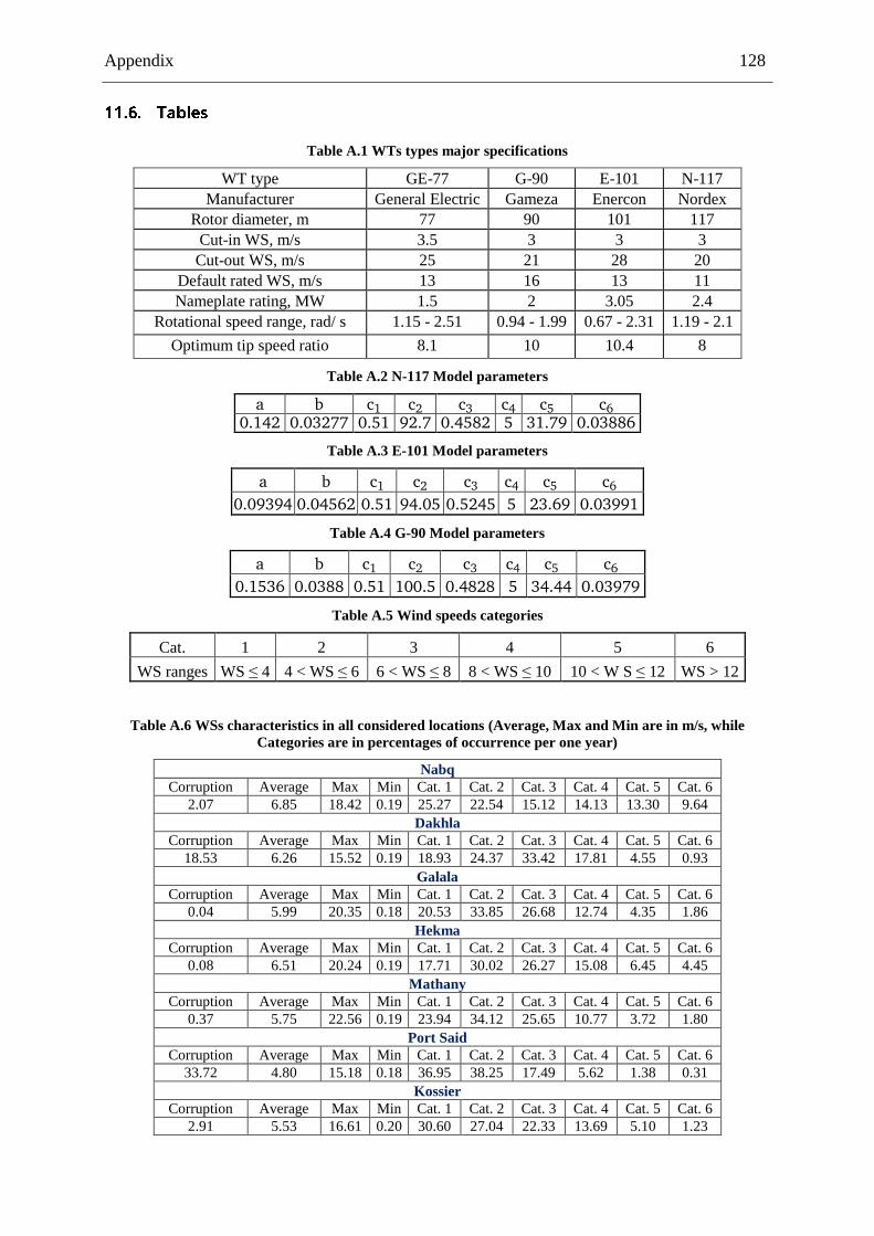
Appendix 128
Table A.1 WTs types major specifications
WT type GE-77 G-90 E-101 N-117
Manufacturer General Electric Gameza Enercon Nordex
Rotor diameter, m 77 90 101 117
Cut-in WS, m/s 3.5 3 3 3
Cut-out WS, m/s 25 21 28 20
Default rated WS, m/s 13 16 13 11
Nameplate rating, MW 1.5 2 3.05 2.4
Rotational speed range, rad/ s 1.15 - 2.51 0.94 - 1.99 0.67 - 2.31 1.19 - 2.1
Optimum tip speed ratio 8.1 10 10.4 8
Table A.2 N-117 Model parameters
a b c1 c2 c3 c4 c5 c6 0.142 0.03277 0.51 92.7 0.4582 5 31.79 0.03886
Table A.3 E-101 Model parameters
a b c1 c2 c3 c4 c5 c6
0.09394 0.04562 0.51 94.05 0.5245 5 23.69 0.03991
Table A.4 G-90 Model parameters
a b c1 c2 c3 c4 c5 c6
0.1536 0.0388 0.51 100.5 0.4828 5 34.44 0.03979
Table A.5 Wind speeds categories
Cat. 1 2 3 4 5 6
WS ranges WS ≤ 4 4 < WS ≤ 6 6 < WS ≤ 8 8 < WS ≤ 10 10 < W S ≤ 12 WS > 12
Table A.6 WSs characteristics in all considered locations (Average, Max and Min are in m/s, while
Categories are in percentages of occurrence per one year)
Nabq
Corruption Average Max Min Cat. 1 Cat. 2 Cat. 3 Cat. 4 Cat. 5 Cat. 6
2.07 6.85 18.42 0.19 25.27 22.54 15.12 14.13 13.30 9.64
Dakhla
Corruption Average Max Min Cat. 1 Cat. 2 Cat. 3 Cat. 4 Cat. 5 Cat. 6
18.53 6.26 15.52 0.19 18.93 24.37 33.42 17.81 4.55 0.93
Galala
Corruption Average Max Min Cat. 1 Cat. 2 Cat. 3 Cat. 4 Cat. 5 Cat. 6
0.04 5.99 20.35 0.18 20.53 33.85 26.68 12.74 4.35 1.86
Hekma
Corruption Average Max Min Cat. 1 Cat. 2 Cat. 3 Cat. 4 Cat. 5 Cat. 6
0.08 6.51 20.24 0.19 17.71 30.02 26.27 15.08 6.45 4.45
Mathany
Corruption Average Max Min Cat. 1 Cat. 2 Cat. 3 Cat. 4 Cat. 5 Cat. 6
0.37 5.75 22.56 0.19 23.94 34.12 25.65 10.77 3.72 1.80
Port Said
Corruption Average Max Min Cat. 1 Cat. 2 Cat. 3 Cat. 4 Cat. 5 Cat. 6
33.72 4.80 15.18 0.18 36.95 38.25 17.49 5.62 1.38 0.31
Kossier
Corruption Average Max Min Cat. 1 Cat. 2 Cat. 3 Cat. 4 Cat. 5 Cat. 6
2.91 5.53 16.61 0.20 30.60 27.04 22.33 13.69 5.10 1.23
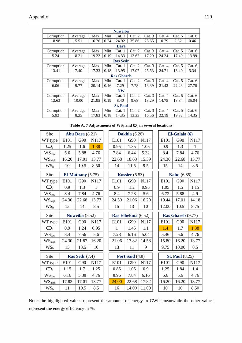
Appendix 129
Nuweiba
Corruption Average Max Min Cat. 1 Cat. 2 Cat. 3 Cat. 4 Cat. 5 Cat. 6
18.98 5.51 16.26 0.24 24.92 35.86 25.65 10.79 2.32 0.46
Dara
Corruption Average Max Min Cat. 1 Cat. 2 Cat. 3 Cat. 4 Cat. 5 Cat. 6
5.24 8.21 19.22 0.19 14.33 12.67 17.29 24.24 17.49 13.99
Ras Sedr
Corruption Average Max Min Cat. 1 Cat. 2 Cat. 3 Cat. 4 Cat. 5 Cat. 6
13.41 7.40 17.33 0.18 13.95 17.07 25.53 24.71 13.40 5.34
Ras Ghareb
Corruption Average Max Min Cat. 1 Cat. 2 Cat. 3 Cat. 4 Cat. 5 Cat. 6
6.06 9.77 20.14 0.16 7.29 7.78 13.39 21.42 22.43 27.70
NW
Corruption Average Max Min Cat. 1 Cat. 2 Cat. 3 Cat. 4 Cat. 5 Cat. 6
13.63 10.00 21.95 0.19 8.40 9.68 13.29 14.75 18.84 35.04
St. Paul
Corruption Average Max Min Cat. 1 Cat. 2 Cat. 3 Cat. 4 Cat. 5 Cat. 6
5.92 8.25 17.83 0.18 14.35 13.23 16.56 22.19 19.32 14.35
Table A. 7 Adjustments of WSb and Ѡb in several locations
Site Abu Dara (8.21)
1
Dakhla (6.26)
1
El-Galala (6)
WT type E101 G90 N117 E101 G90 N117 E101 G90 N117
Ѡb 1.25 1.6 1.38 0.95 1.35 1.05 0.9 1.3 1
WSlow 5.6 5.88 4.76 7.84 6.44 5.32 8.4 7.84 4.76
WShigh 16.20 17.01 13.77 22.68 18.63 15.39 24.30 22.68 13.77
WSb 10 10.5 8.50 14 11.5 9.5 15 14 8.5
Site El-Mathany (5.75) Kossier (5.53) Nabq (6.85)
WT type E101 G90 N117 E101 G90 N117 E101 G90 N117
Ѡb 0.9 1.3 1 0.9 1.2 0.95 1.05 1.5 1.15
WSlow 8.4 7.84 4.76 8.4 7.28 5.6 6.72 5.88 4.9
WShigh 24.30 22.68 13.77 24.30 21.06 16.20 19.44 17.01 14.18
WSb 15 14 8.5 15 13 10 12.00 10.5 8.75
Site Nuweiba (5.52) Ras Elhekma (6.52) Ras Ghareb (9.77)
WT type E101 G90 N117 E101 G90 N117 E101 G90 N117
Ѡb 0.9 1.24 0.95 1 1.45 1.1 1.4 1.7 1.38
WSlow 8.4 7.56 5.6 7.28 6.16 5.04 5.46 5.6 4.76
WShigh 24.30 21.87 16.20 21.06 17.82 14.58 15.80 16.20 13.77
WSb 15 13.5 10 13 11 9 9.75 10.00 8.5
Site Ras Sedr (7.4) Port Said (4.8) St. Paul (8.25)
WT type E101 G90 N117 E101 G90 N117 E101 G90 N117
Ѡb 1.15 1.7 1.25 0.85 1.05 0.9 1.25 1.84 1.4
WSlow 6.16 5.88 4.76 8.96 7.84 6.16 5.6 5.6 4.76
WShigh 17.82 17.01 13.77 24.00 22.68 17.82 16.20 16.20 13.77
WSb 11 10.5 8.5 16 14.00 11.00 10 10 8.50
Note: the highlighted values represent the amounts of energy in GWh; meanwhile the other values
represent the energy efficiency in %.

Appendix 130
Table A.8 Harvested energy in all locations according to the algorithm proposed in Chapter 4
Location Dara
1
Dakhla
1
El-Galala
Season E101 G90 N117 E101 G90 N117 E101 G90 N117
Winter 4.2 3 4.1 1.5 1.2 2.1 1.1 0.8 1.4
63.29 67.80 78.46 22.28 26.64 40.80 15.87 18.20 27.07
Spring 1.7 1.3 2.1 1.7 1.4 2.5 1.1 0.8 1.4
25.10 29.18 39.06 25.24 32.58 47.63 15.89 18.60 27.06
Summer 3.1 2.2 3.1 1.1 0.8 1.5 1.6 1.3 2.2
46.67 50.26 59.50 16.37 19.22 29.03 24.47 28.82 40.96
Fall 3.7 2.6 3.6 1.2 0.9 16.4 1.3 0.9 1.6
54.98 58.70 68.25 17.29 20.94 31.22 18.73 21.42 30.94
Annual 12.7 9 12.9 5.4 4.4 7.8 5 3.8 6.6
47.51 51.49 61.32 20.29 24.85 37.17 18.74 21.76 31.51
Location El-Mathany Kossier Nabq
Season E101 G90 N117 E101 G90 N117 E101 G90 N117
Winter 0.9 0.7 1.1 1.2 1 1.7 2.4 1.7 2.5
13.37 15.24 21.32 18.48 21.71 33.18 35.72 38.49 47.12
Spring 1 0.7 1.3 1.2 1 1.7 2 1.4 2.1
14.47 15.74 24.26 18.39 22.87 32.69 29.20 32.04 39.55
Summer 1.6 1.2 2.1 1.2 0.9 1.7 1.8 1.3 1.8
24.03 27.98 40.53 17.29 20.39 31.84 26.28 28.60 35.15
Fall 1.1 0.8 1.5 0.8 0.6 1.1 2.8 1.9 2.6
15.78 18.63 28.50 12.09 13.96 20.73 42.16 43.82 49.72
Annual 4.5 3.4 6 4.4 0.3 6.2 8.9 6.3 9
16.91 19.40 28.65 16.56 19.73 29.61 33.34 35.74 42.88
Location Nuweiba Ras Elhekma Ras Ghareb
Season E101 G90 N117 E101 G90 N117 E101 G90 N117
Winter 0.9 0.6 1.6 1.3 1 1.7 5.5 3.7 4.8
13.39 14.69 31.22 20.19 23.01 32.74 82.53 84.53 92.21
Spring 0.9 0.7 1.2 1.4 0.9 1.6 4.7 3.2 4.3
14.01 15.28 23.10 20.29 21.74 30.32 70.15 73.27 81.36
Summer 1 0.7 1.4 2.5 1.8 2.7 2.7 1.9 2.9
15.54 17.06 27.02 37.69 40.97 50.75 39.90 44.42 55.63
Fall 1.2 0.9 1.7 1.6 1.1 1.9 4.2 2.9 3.9
17.52 19.98 31.53 23.74 26.12 35.21 63.47 65.82 73.49
Annual 4 0.3 5.9 6.8 4.9 7.8 1.7 1.2 1.6
15.11 16.75 28.22 25.48 27.96 37.26 64.01 67.01 75.67

Appendix 131
Location Ras Sedr Port Said Saint Paul
Season E101 G90 N117 E101 G90 N117 E101 G90 N117
Winter 3.5 2.5 3.8 0.6 0.4 0.7 4 2.9 4
53.10 57.89 71.41 8.88 9.13 13.91 60.44 65.54 77.02
Spring 2.6 1.9 2.9 0.6 0.4 0.7 3.8 2.7 3.7
39.33 43.28 55.10 8.53 8.98 13.89 57.00 61.14 70.95
Summer 1.2 0.9 1.6 0.7 0.5 1 1.7 1.2 1.9
17.59 20.29 30.30 10.98 11.51 18.71 25.45 28.48 36.18
Fall 2.6 1.9 2.8 0.8 0.6 0.1 3.4 2.3 3.2
39.35 42.77 53.48 12.34 12.99 21.02 50.16 53.30 61.38
Annual 10 7.2 1.1 2.7 1.9 3.5 12.9 9.1 12.9
37.34 41.06 52.57 10.18 10.65 16.88 48.26 52.11 61.38
Location ZT NW
Season E101 G90 N117
Winter 5.8 3.9 4.9
87.27 88.13 93.97
Spring 4.6 3.1 4.1
68.66 70.97 78.15
Summer 2.3 1.7 2.5
34.08 37.78 47.72
Fall 4.4 2.9 3.9
65.42 66.81 73.44
Annual 17.1 11.5 15.4
63.86 65.92 73.32
Note: the highlighted values represent the amounts of energy in GWh; meanwhile the other values
represent the energy efficiency in %.
Table A.9 Implementedgovernors’parametersvalues
Steam turbine double reheat
1
Steam turbine single reheat
Parameter value Parameter value
Tch 0.25 s Tch 0.25 s
Tco 0.4 s Tco 0.4 s
Trh1 7.5 s Trh1 7.5 s
Trh2 7.5 s Trh2 7.5 s
Fhp 0.22 Tsr 0.1 s
Fip 0.3 Fhp 0.22
Fvhp 0.22 Fip 0.3
Flp 0.26 Fvhp 0.22
Flp 0.26

Appendix 132
Table A.10 Implemented governors‘ parameters values
Steam governor
1
Hydro mechanical governor
Parameter value Parameter value
T1 2.8 s 0.2 s
T2 5 s Tg 0.2 s
T3 0.15 s Tp 0.045 s
Valve rate limits Gate rate limits
Increasing 0.2 pu Increasing 0.2 pu
Decreasing -1 pu Decreasing -0.2 pu
Valve opening Gate opening
Max 1 Max 1
Min 0 Min 0
Table A.11 Implemented governors‘ parameters values
Hydro Woodward PID governor
1
Hydro electronic governor
Parameter value Parameter value
Ka 1 Ka 5
Kd 1.5 Kd 0.8
Kp 3.2 Ta 0.05 s
Ksm 4 Td 0.2 s
Tc 0.1 s Tw 0.55 s
Td 0.02 s beta 0.5
Gate rate limits Gate rate limits
Increasing 0.1 pu Increasing 0.1 pu
Decreasing -0.1 pu Decreasing -0.1 pu
Gate opening limits Gate opening
Max 0.95 Max 0.95
Min 0 Min 0
Table A.12 Load model and AGC parameters
Load model
1
AGC
Parameter value Parameter value
Dl (static load component) 1/200 Hz/MW CpAGC 0.17
Wo (Dynamic load component) 100 MW/Hz Tn 120
K 8
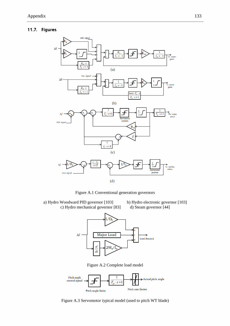
Appendix 133
Figure A.1 Conventional generation governors
a) Hydro Woodward PID governor [103] b) Hydro electronic governor [103]
c) Hydro mechanical governor [83] d) Steam governor [44]
Figure A.2 Complete load model
Figure A.3 Servomotor typical model (used to pitch WT blade)

Publications 134
A. B. Attya, T. Hartkopf, Wind turbines support techniques during frequency drops — Energy
utilization comparison, AIMS Energy Journal, vol. 2, no. 3, pp. 219-234, 2014.
A. B. Attya, T. Hartkopf, Wind turbine contribution in frequency drop mitigation – Modified
operation and estimating released supportive energy, IET Journal of Generation, Transmission
and Distribution, vol. 8, no. 5, pp. 862-872, May 2014.
A. B. Attya, T. Hartkopf, Wind farms dispatching to manage the activation of frequency
support algorithms embedded in connected wind turbines, International Elsevier Journal of
Electrical Power and Energy Systems, vol. 53, issue 1, December 2013.
A. B. Attya, T. Hartkopf, Control and quantification of kinetic energy released by wind farms
during power system frequency drops, IET Renewable Power Generation, vol. 7, issue 3, May
2013.
A. B. Attya, T. Hartkopf, Penetration impact of wind farms equipped with frequency
variations ride through algorithm on power system frequency response, Elsevier International
Journal of Electrical Power and Energy Systems, vol. 40, issue 1, September 2012.
A. B. Attya, T. Hartkopf, Wind energy in Egypt- Capacity assessment and analyzing
penetration impact on grid frequency, in proc. of IEEE 4th International conference on Power
Engineering, Energy and Electrical Drives, Istanbul, 2013.
A. B. Attya, T. Hartkopf, Estimation of wind turbines dynamic model parameters using
published manufacturer product data, in proc. of IEEE International Energy Conference and
Exhibition, Florence, 2012.
A. B. Attya, T. Hartkopf, Generation of high resolution wind speeds and wind speed arrays
inside a wind farm based on real site data, in proc. of IEEE 11th conference on Electrical
Power Quality and Utilization, Lisbon, October 2011.

Acknowledgement 135
All praise and thanks to Allah
Special thanks to my respectable supervisors Prof. Hartkopf, Prof. Griepentrog, and Prof. Hegazy
Special thanks to my friend and ex-colleague Dr. Peter Engel
Special thanks for the DAAD (Deutscher Akademischer Austausch Dienst), and the Egyptian ministry
of high education and research who funded my PhD scholarship.
Special thanks to Prof. Hegazy who provided me with valuable data about the Egyptian case study.
Thanks to my parents, my wife, my children and my friends who supported me, and kept their patience
and prayers through the road towards this valuable degree.
Thanks to my colleagues in the department.

Academic career 136
German Egyptian Research Long term scholarship (GERLS)- [01.10.2011 till now]
Full PhD scholarship at the Technical University of Darmstadt, at the department of Renewable
Energies. Thesis topic: Wind energy penetration impact on grid frequency during normal
operation and frequency drops
Part time research assistant – Technical University of Darmstadt [01.12.2012 till now]
Tutor and instructor in undergraduate and postgraduate tutorials beside the supervision of master
students. Courses: Renewable Energies and Efficient use of Energy
Research Assistant – GUC (German University in Cairo) - [05.9.2006 -30.9.2010]
Tutor and instructor in undergraduate and postgraduate tutorials and labs in the faculty of
Information Engineering and Technology (IET), besides the supervision of the bachelor projects.
Courses: Power Electronics, Electrical Circuits I, Electrical Circuits II and Advanced power
electronics lab.
M. Sc. in Electrical Power Engineering, Faculty of Engineering, Ain Shams University. Thesis
title: Impact of Distributed Generation Technology on Distribution System Reliability [May
2008]
B. Sc. in Electrical Power Engineering, faculty of engineering, Ain Shams University. Grade:
Very Good with Honour (ranked 11th over 280 students) [July 2005].
High school education at Saint Fatima language school, (English as a first Language, French
as a second language), Secondary certificate (Grade: 98%) [July 2000]
Adequacy analysis of distributed generation, and offered methodologies to judge the system
performance. MATLAB codes were developed to estimate reliability indices based on Monte Carlo
simulation. Different generation techniques were examined. Cost-worth reliability evaluation was
implemented in an attempt to judge on the feasibility of any modifications that could be applied in a
given power network.