Embed Size (px)
Citation preview

PhD Topics in Macroeconomics
Lecture 1: introduction and course overview
Chris Edmond
2nd Semester 2014
1

Introduction
• A course ‘the whole family can enjoy’
• Research on firm heterogeneity takes place at the intersection ofmacro, trade, IO, labor etc
• Papers typically integrate micro-data and theory
– data guiding model development, and
– data examined through the lens of models
2

Introduction
• We will begin with classic papers on firm dynamics per se
• Then turn to more recent applications/extensions, including
– innovation and aggregate growth
– misallocation and cross-country income differences
– heterogeneous firms and international trade
3

Course requirements
• Four problem sets, 10% each
• Two referee report, 10% each, due Monday Oct 20th
• Research proposal presentation, 40%, beginning Monday Oct 27th
4
Overview
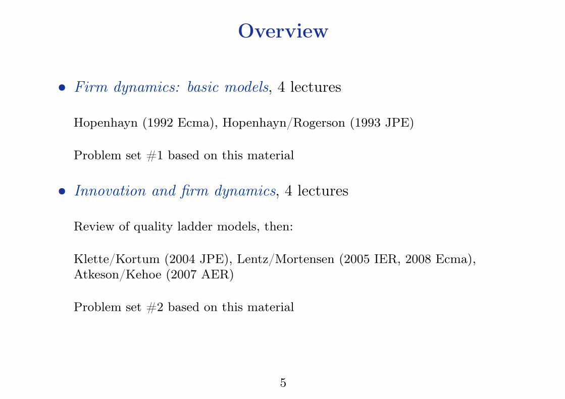
• Firm dynamics: basic models, 4 lectures
Hopenhayn (1992 Ecma), Hopenhayn/Rogerson (1993 JPE)
Problem set #1 based on this material
• Innovation and firm dynamics, 4 lectures
Review of quality ladder models, then:
Klette/Kortum (2004 JPE), Lentz/Mortensen (2005 IER, 2008 Ecma),Atkeson/Kehoe (2007 AER)
Problem set #2 based on this material
5
Overview
• Misallocation, 4 lectures
Restuccia/Rogerson (2008 RED), Hsieh/Klenow (2009 QJE),Peters (2013wp), Buera/Shin (2013 JPE), Midrigan/Xu (2014 AER)
Problem set #3 based on this material
• Heterogeneous firms and international trade, 6 lectures
Review of monopolistic competition and trade, then:
Melitz (2003 Ecma), Chaney (2008 AER), Eaton/Kortum (2002 Ecma)Bernard/Eaton/Jensen/Kortum (2003 AER), Eaton/Kortum/Kramarz(2011 Ecma)
Problem set #4 based on this material
6
Overview
• Aggregate gains from trade, 3 lectures
Arkolakis/Costinot/Rodriguez-Clare (2012 AER),Arkolakis/Costinot/Donaldson/Rodriguez-Clare (2012wp),Edmond/Midrigan/Xu (2014wp)
• ‘Thoughts on Piketty’, 3 lectures
Piketty (2014, selections), Atkinson/Piketty/Saez (2011 JEL),Piketty/Zucman (2014 QJE), Benhabib/Bisin/Zhu (2013wp)
What’s the connection? Pareto distributions, distributional dynamics etc.
7
Firm dynamics: basic models, part one
Rest of today’s class:
• Background facts on firm-size distribution
– Zipf’s law and Gibrat’s law as organizing principles
• Simple models of the firm-size distribution
– statistical models
* Yule/Simon preferential attachment
– economic models
* Lucas span of control
8
Two empirical benchmarks
1- Zipf’s law :
– frequency of observation inversely proportional to rank
(word-use, city-size, firm-size, . . . )
2- Gibrat’s law :
– individual firm growth rates independent of size
(at least, for large enough firms)
How are these related?
9
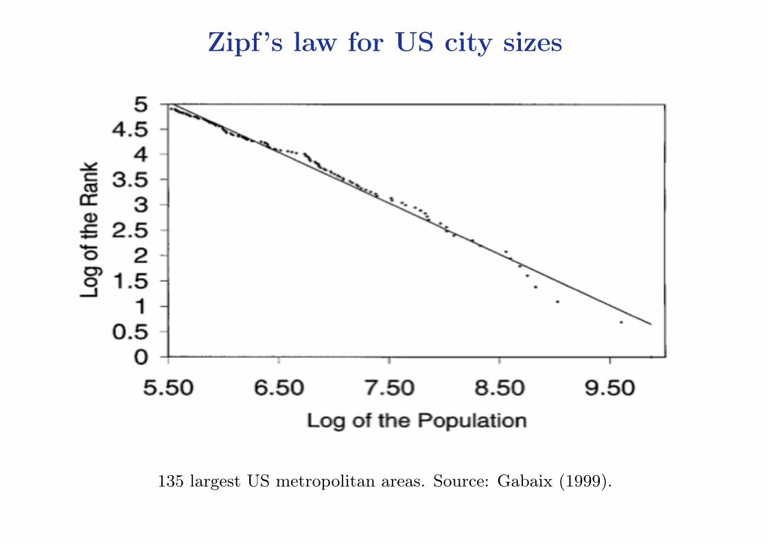
Zipf’s law for US city sizes
135 largest US metropolitan areas. Source: Gabaix (1999).
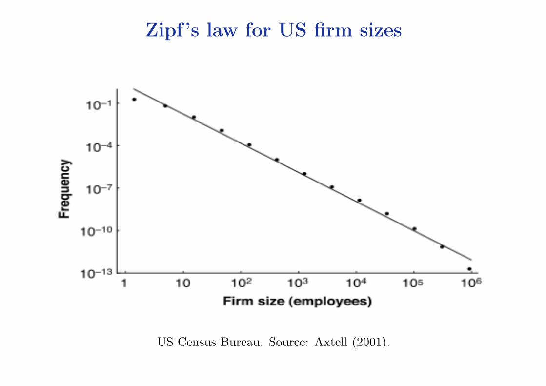
Zipf’s law for US firm sizes
US Census Bureau. Source: Axtell (2001).
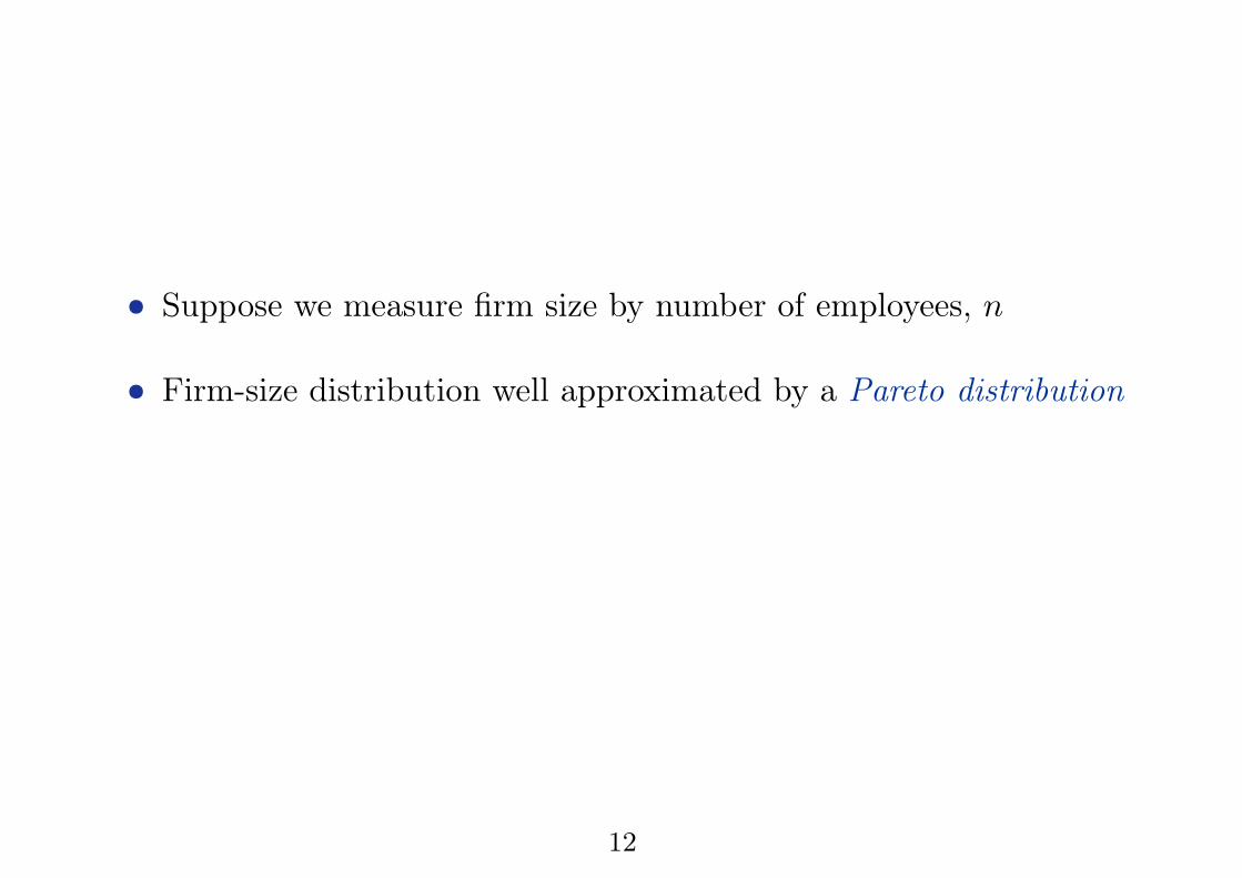
• Suppose we measure firm size by number of employees, n
• Firm-size distribution well approximated by a Pareto distribution
12
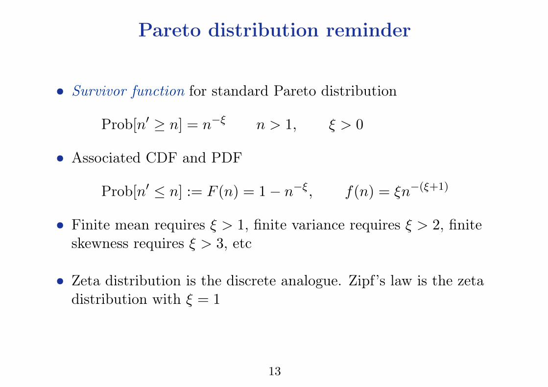
Pareto distribution reminder
• Survivor function for standard Pareto distribution
Prob[n0 � n] = n
�⇠
n > 1, ⇠ > 0
• Associated CDF and PDF
Prob[n0 n] := F (n) = 1� n
�⇠
, f(n) = ⇠n
�(⇠+1)
• Finite mean requires ⇠ > 1, finite variance requires ⇠ > 2, finiteskewness requires ⇠ > 3, etc
• Zeta distribution is the discrete analogue. Zipf’s law is the zetadistribution with ⇠ = 1
13
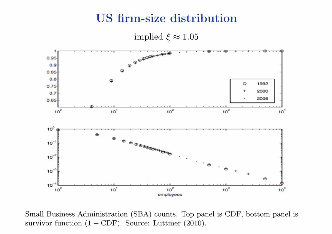
US firm-size distributionimplied ⇠ ⇡ 1.05
Small Business Administration (SBA) counts. Top panel is CDF, bottom panel issurvivor function (1� CDF). Source: Luttmer (2010).

Repeated cross-sections
Business Dynamics Statistics (BDS) categories. Source: Luttmer (2010).

• In short, US firm-size distribution is both very stable and veryskewed
– there are about 6 million firms
– around one-half of total employment is accounted for by some
18,000 very large firms with more than 500 employees each
– around one-quarter of total employment is accounted for by some
1,000 enormous firms with more than 10,000 employees each
– but most firms are small, almost 80% of firms have less than 10
employees
• Perhaps surprisingly, a stable firm-size distribution is the fairlynatural consequence of random growth at the micro level (almost)
16
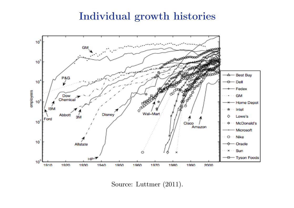
Individual growth histories
Source: Luttmer (2011).

Gibrat’s law
• Starting point: Gibrat’s law of ‘proportional effect’
• Fixed population of units i (cities, firms, . . . ) of size P
i
t
• Let Si
t
:= P
i
t
/
¯
P
t
denote normalized size (relative to average size ¯
P
t
)and suppose
S
i
t+1 = �
i
t
S
i
t
�
i
t
⇠ IID f(�) (1)
Growth independent of current size, so absolute incrementS
t+1 � S
t
approximately proportional to current size S
t
• Let G
t
(x) := Prob[Si
t
� x] denote the survivor function
18
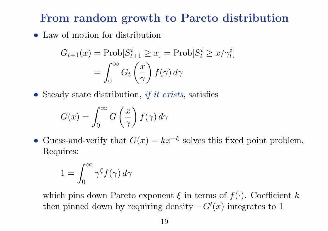
From random growth to Pareto distribution• Law of motion for distribution
G
t+1(x) = Prob[Si
t+1 � x] = Prob[Si
t
� x/�
i
t
]
=
Z 1
0G
t
✓x
�
◆f(�) d�
• Steady state distribution, if it exists, satisfies
G(x) =
Z 1
0G
✓x
�
◆f(�) d�
• Guess-and-verify that G(x) = kx
�⇠ solves this fixed point problem.Requires:
1 =
Z 1
0�
⇠
f(�) d�
which pins down Pareto exponent ⇠ in terms of f(·). Coefficient k
then pinned down by requiring density �G
0(x) integrates to 1
19

Existence of a steady-state distribution
• Of course there need not be a steady-state distribution
• Suppose f(�) is log-normal, ln � ⇠ N(µ,�
2), then
lnS
i
t
� lnS
i
0 ⇠ N(µt,�
2t)
and there is no steady-state distribution, it keeps fanning out
• But turns out that ‘small departures’ from this strict version ofGibrat’s law give us back a steady-state distribution and moreovergive micro foundations for ⇠ ⇡ 1
Examples: Gabaix (1999 QJE), Luttmer (2007 QJE)
20
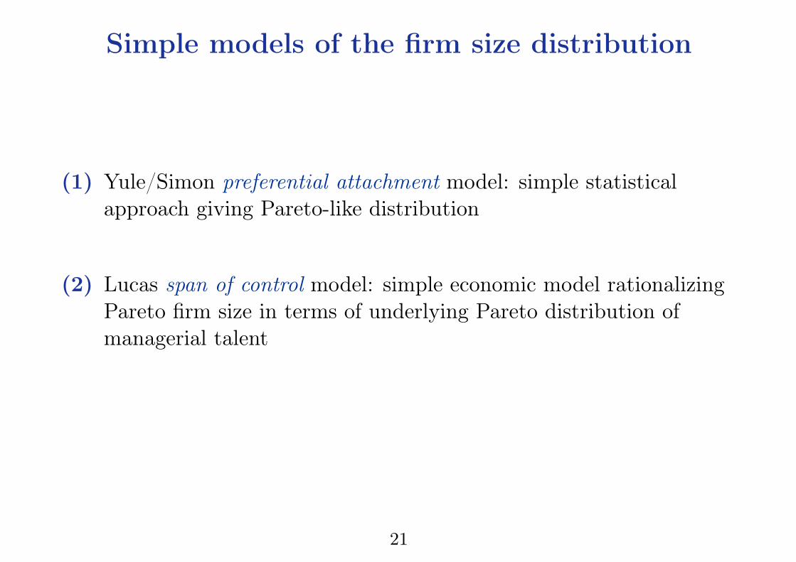
Simple models of the firm size distribution
(1) Yule/Simon preferential attachment model: simple statisticalapproach giving Pareto-like distribution
(2) Lucas span of control model: simple economic model rationalizingPareto firm size in terms of underlying Pareto distribution ofmanagerial talent
21
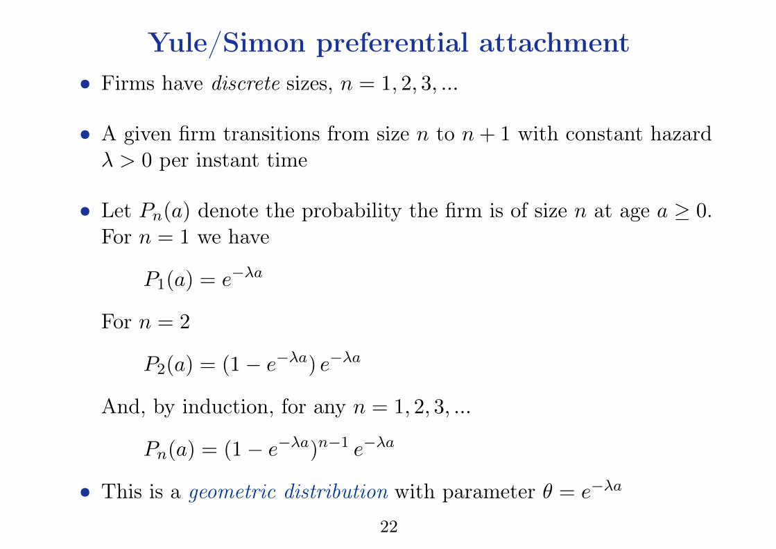
Yule/Simon preferential attachment• Firms have discrete sizes, n = 1, 2, 3, ...
• A given firm transitions from size n to n+ 1 with constant hazard� > 0 per instant time
• Let P
n
(a) denote the probability the firm is of size n at age a � 0.For n = 1 we have
P1(a) = e
��a
For n = 2
P2(a) = (1� e
��a
) e
��a
And, by induction, for any n = 1, 2, 3, ...
P
n
(a) = (1� e
��a
)
n�1e
��a
• This is a geometric distribution with parameter ✓ = e
��a
22

Yule/Simon distribution
• The cross-sectional firm-size distribution is then given by
P
n
:=
Z 1
0P
n
(a)f(a) da
where f(a) is the PDF of firm ages
• Suppose age has exponential distribution with parameter �. Then
P
n
=
Z 1
0P
n
(a) �e
��a
da =
Z 1
0(1� e
��a
)
n�1e
��a
�e
��a
da
=
�
�
Z 1
0(1� ✓)
n�1✓
�/�
d✓
(making change of variables to the geometric paramater ✓ = e
��a)
23

Yule/Simon distribution• Recall the beta and gamma functions
B(x, y) :=
Z 1
0✓
x�1(1� ✓)
y�1d✓, �(x) :=
Z 1
0✓
x�1e
�✓
d✓
The gamma function �(x) is the continuous analogue of thefactorial function, x�(x) = �(x+ 1) etc
• These are related by
B(x, y) =
�(x)�(y)
�(x+ y)
• So the firm-size distribution can be written
P
n
= (�/�)B
⇣(�/�) + 1, n
⌘= (�/�)
�((�/�) + 1)�(n)
�((�/�) + 1 + n)
This is the Yule/Simon distribution with parameter �/�.
24
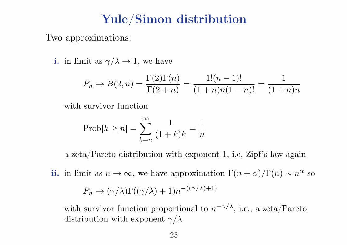
Yule/Simon distributionTwo approximations:
i. in limit as �/� ! 1, we have
Pn ! B(2, n) =
�(2)�(n)
�(2 + n)
=
1!(n� 1)!
(1 + n)n(1� n)!
=
1
(1 + n)n
with survivor function
Prob[k � n] =
1X
k=n
1
(1 + k)k
=
1
n
a zeta/Pareto distribution with exponent 1, i.e, Zipf’s law again
ii. in limit as n ! 1, we have approximation �(n+ ↵)/�(n) ⇠ n
↵so
Pn ! (�/�)�((�/�) + 1)n
�((�/�)+1)
with survivor function proportional to n
��/�, i.e., a zeta/Pareto
distribution with exponent �/�
25

Lucas 1978 span of control
• Firm consists of a production technology and a managerialtechnology
• Production technology is standard concave CRS
y = F (k, n) = f(k/n)n
• Managerial technology: manager of talent x produces
x g(y)
units of output where g(·) is strictly increasing, strictly concave
• Manager is a fixed input. DRS of g(·) reflects their limited span ofcontrol – best manager can’t control everything. Efficient for someresources to be controlled by next-best manager, etc
26
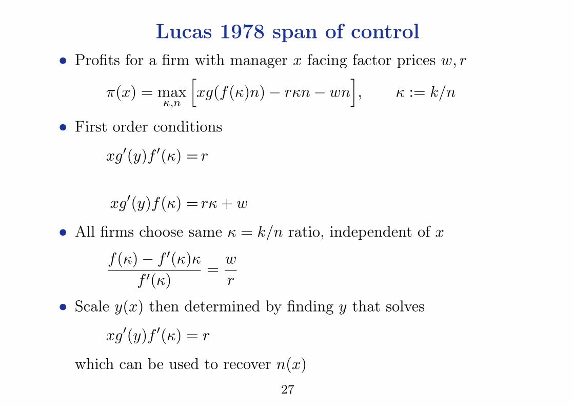
Lucas 1978 span of control• Profits for a firm with manager x facing factor prices w, r
⇡(x) = max
,n
hxg(f()n)� rn� wn
i, := k/n
• First order conditions
xg
0(y)f
0() = r
xg
0(y)f() = r+ w
• All firms choose same = k/n ratio, independent of x
f()� f
0()
f
0()
=
w
r
• Scale y(x) then determined by finding y that solves
xg
0(y)f
0() = r
which can be used to recover n(x)
27

Implications of Gibrat’s law
• Firm growth induced by changes in factor prices
d
dt
ln[n(x ; w(t), r(t))] =
n
w
(x,w, r)
n(x,w, r)
w
0(t) +
n
r
(x,w, r)
n(x,w, r)
r
0(t)
• Strong form of Gibrat’s law is hypothesis that this derivative isinvariant to firm size
@
@x
hn
w
(x,w, r)
n(x,w, r)
w
0(t) +
n
r
(x,w, r)
n(x,w, r)
r
0(t)
i= 0
• For this to hold for all patterns of changing factor prices, musthave both
@
@x
n
w
(x,w, r)
n(x,w, r)
=
@
@x
n
r
(x,w, r)
n(x,w, r)
= 0
28

Implications of Gibrat’s law
• The condition
@
@x
n
w
(x,w, r)
n(x,w, r)
= 0
is implicitly a restriction on the functional form of g(·)
• Calculating n
w
(x,w, r) and solving the differential equation forg(·), Lucas finds that
g(y) = Ay
↵
, A > 0, 0 < ↵ < 1
is the unique functional form consistent with the strong version ofGibrat’s law
29

Lucas 1978 example
• Suppose the production function y = n, the managerial technologyxy
↵ and that managerial talent has the Pareto distribution withCDF 1� x
�⇠
• First order condition
x↵y
↵�1= w ) y(x) = n(x) =
⇣↵x
w
⌘1/(1�↵)
• Hence if managerial talent has Pareto distribution with exponent⇠, then firm-size is also Pareto with exponent ⇠(1� ↵)
30

Managerial selection
• Suppose individual of talent x can opt for wage w or manage andearn income ⇡(x)
• Indifference condition
⇡(x) = xg[f()n(x)]� rn(x)� wn(x) = w
• Cutoff managerial type x
⇤ such that only x > x
⇤ actively manage
x
⇤g[f()n(x
⇤)] = w + (rn(x
⇤) + wn(x
⇤))
i.e., fixed cost w (opportunity cost of manager) plus variable costs
31

Next
• Firm dynamics: basic models, part two
⇧ Hopenhayn (1992): Entry, exit and firm dynamics in long run
equilibrium, Econometrica.
32