Embed Size (px)
Citation preview
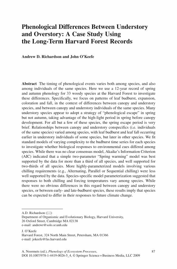
Phenological Differences Between Understory and Overstory: A Case Study Using the Long-Term Harvard Forest Records
Andrew D. Richardson and John O’Keefe
Abstract The timing of phenological events varies both among species, and also among individuals of the same species. Here we use a 12-year record of spring and autumn phenology for 33 woody species at the Harvard Forest to investigate these differences. Specifically, we focus on patterns of leaf budburst, expansion, coloration and fall, in the context of differences between canopy and understory species, and between canopy and understory individuals of the same species. Many understory species appear to adopt a strategy of “phenological escape” in spring but not autumn, taking advantage of the high-light period in spring before canopy development. For all but a few of these species, the spring escape period is very brief. Relationships between canopy and understory conspecifics (i.e. individuals of the same species) varied among species, with leaf budburst and leaf fall occurring earlier in understory individuals of some species, but later in other species. We fit standard models of varying complexity to the budburst time series for each species to investigate whether biological responses to environmental cues differed among species. While there was no clear consensus model, Akaike’s Information Criterion (AIC) indicated that a simple two-parameter “Spring warming” model was best supported by the data for more than a third of all species, and well supported for two-thirds of all species. More highly-parameterized models involving various chilling requirements (e.g., Alternating, Parallel or Sequential chilling) were less well supported by the data. Species-specific model parameterization suggested that responses to both chilling and forcing temperatures vary among species. While there were no obvious differences in this regard between canopy and understory species, or between early- and late-budburst species, these results imply that species can be expected to differ in their responses to future climate change.
A.D. Richardson (*)Department of Organismic and Evolutionary Biology, Harvard University, 26 Oxford Street, Cambridge MA 02138 e-mail: [email protected]
J. O’KeefeHarvard Forest, 324 North Main Street, Petersham, MA 01366 e-mail: [email protected]
A. Noormets (ed.), Phenology of Ecosystem Processes, 87DOI 10.1007/978-1-4419-0026-5_4, © Springer Science + Business Media, LLC 2009
88 A.D. Richardson and J. O’Keefe
1 Introduction
Plants exhibit both phenotypic plasticity and genotypic adaptation to different growth environments (Schlichting 1986 ; Sultan 1995) . In terms of phenology, these responses can be manifest as differences in spring budburst and autumn senescence within species across environmental gradients at varying scales, from regional (e.g., across the native range of a species; see Lechowicz 1984 ; Raulier and Bernier 2000) to local (e.g., along an elevational gradient: see Richardson et al. 2006) and even microsite (e.g., with regard small-scale topographic variation and cold air drainage, see Fisher et al. 2006) . These patterns are commonly interpreted in the context of differences in temperature regime among different growth environments.
However, just as differences in light environment between understory and canopy result in well-known differences in leaf structure (Boardman 1977 ; Lichtenthaler et al. 1981) , so too can plants respond to the ambient light environment by adopting different phenological strategies. For example, many herbaceous understory species in temperate deciduous forests have been shown to adopt “phenological escape” (Crawley 1997) strategies of shade avoidance in order to increase the seasonal integral of potential photosynthesis and to capitalize on other seasonally-limited resources for growth (e.g., Muller 1978) . By emerging earlier in the spring than canopy species (or by delaying autumn senescence), shade-avoiding understory plants can take advantage of a short-lived high-light growth environment (e.g., Sparling 1967 ; Mahall and Bormann 1978 ; Crawley 1997) . As demonstrated by greenhouse studies, early-emerging individuals not only have more time to grow, but also grow more quickly and accumulate more resources than individuals that emerge later (Rathcke and Lacey 1985) . Textbook examples of herbaceous species adopting the escape strategy include Hyacinthoides non-scripta and Anemone nemorosa (Crawley 1997) . Such a strategy is not without tradeoffs, however: early-emerging individuals often have a lower chance of survival, but much higher repro-ductive success, than individuals that emerge later (Rathcke and Lacey 1985) . Earlier emergence increases susceptibility to spring frost damage which may not only damage photosynthetic machinery but also lead to foliar necrosis (e.g., Gu et al. 2008) . Also, plants that emerge under high-light conditions may not be morphologi-cally well-adapted to low light conditions. For example, work by Sparling (1967) demonstrated that herbs emerging in spring, prior to canopy closure, had photosyn-thetic characteristics of shade intolerant species, whereas species emerging in mid-summer exhibited shade tolerant characteristics (see also Hull 2002) . However, Rothstein and Zak (2001) reported that acclimation of individual leaves could occur as the growing season progressed and the below-canopy light environment changed: leaves of Viola pubescens emerged prior to canopy closure with sun leaf character-istics, but as the canopy closed, both chemical (e.g., N partitioning to Rubisco vs. chlorophyll) and structural (leaf mass to area ratio) acclimation resulted in the same leaves becoming more like shade leaves, and thus better suited to a low-light environment.
While phenological escape is well-documented for herbaceous species, much less is known about the degree to which this strategy is adopted by woody plants,
Phenological Differences Between Understory and Overstory 89
either shrub/small tree species restricted to the understory, or juvenile/suppressed individuals of canopy species. Previous work in this regard has generally been focused on a relatively limited number of species, and results have not been entirely consistent among studies. While the overall pattern is one of understory species and juveniles of canopy species leafing out earlier in spring, but not necessarily dropping their leaves later in autumn, than mature canopy trees (Gill et al. 1998 ; Seiwa 1999a, b ; Augspurger and Bartlett 2003 ; Barr et al. 2004 ; Augspurger et al. 2005) , important questions remain. For example, how widespread is the phenological escape strategy among woody understory plants? Or, what traits do species adopting this strategy have in common? And, are there differences between understory species and juveniles of canopy species in terms of how this strategy is expressed?
In the sections that follow, we begin by providing a brief review of how the understory growth environment varies from season to season. We then discuss evidence for phenological variation within and among species, first broadly and then specifically with regard to differences between understory and canopy. This is followed by an evaluation of potential fitness consequences of different phenological strategies. We then use data from the long-term phenology records maintained at the Harvard Forest as a case study to investigate the following questions in the context of patterns of spring (budburst and leaf expansion) and autumn (leaf coloration and leaf fall) phenology for an entire forest community, comprising 33 different woody species:
1. Are there differences in phenology between understory tree and shrub species and canopy tree species (i.e., those that have the potential to grow into the canopy)?
2. Within the class of canopy species, are there differences in phenology between suppressed individuals growing in the understory, and dominant or co-dominant individuals in the overstory?
3. Given that year-to-year variation in weather (e.g., warm vs. cool spring) gener-ally results in corresponding shifts in the timing of phenological events (Hunter and Lechowicz 1992) , how do species differ in their sensitivities to climatic vari-ability? For example:
(a) Is the sequence in which species reach particular phenophases consistent from year to year?
(b) Are there differences among species (particularly with regard to canopy vs. understory species) in terms of which temperature-based model to predict budburst is best supported by the data?
1.1 Seasonal Variation in the Understory Growth Environment
The seasonal patterns of light availability for various canopy strata in a temperate deciduous forest depend largely on the development and senescence of the overstory canopy (throughout this remainder of this chapter we use “canopy” and “overstory” as
90 A.D. Richardson and J. O’Keefe
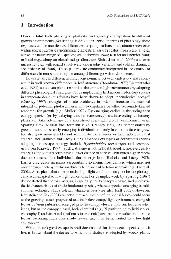
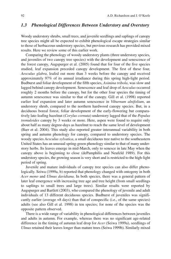
synonyms), with changing zenith angle and overall solar irradiance acting as sec-ondary factors (Baldocchi et al. 1984) . As an example, data from the Bartlett Experimental Forest, a northern hardwood (maple-beech-birch) forest in central New Hampshire, indicate a rapid spring decrease in the fraction of photosyntheti-cally active radiation transmitted through the canopy ( f
TPAR ) as the developmental
trajectory progresses from a leafless (day 121 in Fig. 1a ) to a fully-foliated (day 165 in Fig. 1a ) canopy. Over a period of roughly 1 month, f
TPAR declines from ~ 50% to
~ 5% (Fig. 1b , see also Baldochi et al. 1986 ; Gill et al. 1998) . During this time the understory light environment is extremely heterogeneous, as canopy species leaf out at different times and leaf elongation proceeds at different rates (Kato and Komiyama 2002) . With canopy closure, sunflecks become ever more important for understory photosynthesis (Chazdon and Pearcy 1991) . In the autumn, the reverse pattern occurs, over a similarly brief period, with the onset of leaf senescence and, ultimately, abscission. It is important to note that the physical presence of the canopy does not necessarily mean the canopy is physiologically active (Sakai et al. 1997) : particularly in the autumn, canopy photosynthesis is reduced with the onset of
Day 121 Day 138 Day 165
a
b
Fig. 1 Rapid changes in the state of the canopy ( a ) affect the below-canopy light environment ( b ), as measured by f
TPAR = Q
transmitted / Q
incident , the fraction of incident photosynthetically active
radiation that is transmitted through the canopy. Data from the Bartlett Experimental Forest, White Mountain National Forest, New Hampshire. Photo credit: Chris Costello.
Phenological Differences Between Understory and Overstory 91
senescence, but shading of the understory continues until canopy leaves are actually dropped.
Beyond fluxes of photosynthetically active radiation, the presence or absence of a full canopy affects other aspects of energy and mass transfer, with implications for various factors affecting growth and development of understory plants, including: leaf temperatures and saturation deficit; precipitation throughfall as well as soil surface heat flux and evaporation; and diurnal ranges of air and soil temperatures.
1.2 Phenological Differences Within and Among Species
For a given tree species, climatic gradients (particularly latitude but also elevation) are a dominant control on phenology, as budburst by higher-latitude and higher-elevation individuals generally follows that of lower-latitude and lower-elevation individuals (e.g., Lechowicz 1984 ; Richardson et al. 2006 ; Fisher et al. 2007) . This can be attributed to varying rates of spring warming, as temperature is considered the primary trigger for spring budburst, at least in temperate, boreal, and arctic ecosystems. However, provenance trials indicate that there is genetic variation among populations in terms of responsiveness to environmental cues. For example, in common-garden experiments, northern populations have generally been shown to leaf out in advance of southern populations, although the reverse is true in some species (Lechowicz 1984) .
In temperate forests, coexisting tree species commonly leaf out at different times, from the typically early emergence of Betula and Populus , to the late emergence of Quercus and Fraxinus . Among these species, budburst dates vary by 3 weeks or more in a temperate deciduous forest in Quebec, although a similar ordering of related species is observed both elsewhere in North America and also in Europe (Lechowicz 1984) . At the same time, the rate of canopy development also differs among species, with leaf elongation proceeding rapidly in some species ( Prunus and Acer ) but more slowly in other species ( Juglans and Carya ) (Lechowicz 1984) . Perhaps surprisingly, the timing of budburst is not correlated with ecological niche (e.g., shade tolerance) or with phylogenetic history (both advanced and primitive families can be either early or late leafing out, and within families, and even within genera, there is just as much variation as among families); however, noting that many late-leafing tree species tended to be ring-porous (i.e., woody species in which the xylem vessels laid down at the beginning of the growing season are much larger in diameter than those produced later in the growing season), Lechowicz (1984) hypothesized that ring-porous species leaf out later than diffuse-porous species because large diameter vessels are more prone to cavitation caused by freeze-thaw xylem embolism. Thus in ring-porous species budburst can only occur after new xylem has been formed each spring, as otherwise there would be little or no capacity to transport water to developing leaves. In diffuse-porous species, on the other hand, the hydraulic conductivity is less affected by winter freezing, and leaf development can occur in advance of, or concurrently with, the formation of new xylem.
92 A.D. Richardson and J. O’Keefe
1.3 Phenological Differences Between Understory and Overstory
Woody understory shrubs, small trees, and juvenile seedlings and saplings of canopy tree species might all be expected to exhibit phenological escape strategies similar to those of herbaceous understory species, but previous research has provided mixed results. Here we review some of this earlier work.
Comparing the phenology of woody understory plants (three understory species, and juveniles of two canopy tree species) with the development and senescence of the forest canopy, Augspurger et al. (2005) found that for four of the five species studied, leaf expansion preceded canopy development. The first of these four, Aesculus glabra , leafed out more than 3 weeks before the canopy and received approximately 97% of its annual irradiance during this spring high-light period. Budburst and foliar development of the fifth species, Asimina tribola , was slow and lagged behind canopy development. Senescence and leaf drop of Aesculus occurred roughly 2 months before the canopy, but for the other four species the timing of autumn senescence was similar to that of the canopy. Gill et al. (1998) reported earlier leaf expansion and later autumn senescence in Viburnum alnifolium , an understory shrub, compared to the northern hardwood canopy species. But, in a deciduous boreal forest, foliar development of the early-flowering but compara-tively late-leafing hazelnut ( Corylus cornuta ) understory lagged that of the Populus tremuloides canopy by 3 weeks or more. Here, aspen were found to require only about half as many degree-days as hazelnut to reach the same level of development (Barr et al. 2004) . This study also reported greater interannual variability in both spring and autumn phenology for canopy, compared to understory species. The woody species Aesculus sylvatica , a small deciduous tree native to the southeastern United States has an unusual spring-green phenology similar to that of many under-story herbs. Its leaves emerge in mid-March, only to senesce in late May when the canopy above is beginning to close (dePamphilis and Neufeld 1989) . For this understory species, the growing season is very short and is restricted to the high-light period of spring.
Juvenile and mature individuals of canopy tree species can also differ pheno-logically. Seiwa (1999a, b) reported that phenology changed with ontogeny in both Acer mono and Ulmus davidiana . In both species, there was a general pattern of later leaf emergence with increasing tree age and tree height (from small seedlings to saplings to small trees and large trees). Similar results were reported by Augspurger and Bartlett (2003) , who compared the phenology of juvenile and adult individuals of 13 different deciduous species. Budburst of juveniles was signifi-cantly earlier (average » 8 days) than that of conspecific (i.e., of the same species) adults (see also Gill et al. 1998) in ten species; for none of the species was the opposite pattern observed.
There is a wide range of variability in phenological differences between juveniles and adults in autumn. For example, whereas there was no significant age-related difference in the timing of autumn leaf drop for Acer (Seiwa 1999a) , seedlings of Ulmus retained their leaves longer than mature trees (Seiwa 1999b) . Similarly mixed
Phenological Differences Between Understory and Overstory 93
results were presented by Augspurger and Bartlett (2003) , who reported that for most of the 13 species studied, the timing of onset of senescence and completion of leaf fall did not vary between juveniles and adults. Where significant differences were observed, the pattern of variation was not consistent among species: juveniles retained their leaves longer in some instances (e.g. Acer saccharum ), but shorter in others (e.g. Aesculus glabra ). In contrast to these results, Gill et al. (1998) found that understory Acer saccharum and Fagus grandifolia retained green leaves later in autumn than overstory trees of the same species.
On the basis of the springtime patterns, Seiwa (1999a, b) suggested that the overall net benefits of earlier leaf-out must therefore decrease with increasing tree height, reflecting a shifting balance between the advantages (increased carbon gain and reduced susceptibility to herbivory, e.g., Crawley 1997) and the disadvantages (risk of frost damage, e.g., Lechowicz 1984) of early leaf out. This would seem to be a logical explanation: for individuals deep under the canopy, leafing out early offers the largest rewards. By comparison, for dominant canopy trees, the competi-tion for light has already been “won”, and leafing out early is of much less benefit. Thus, one would predict that leaf expansion “progress from the base of the canopy upward” but autumn senescence “[progress] from the top of the canopy downward” (Gill et al. 1998) .
1.4 Consequences of Different Phenological Strategies
Studies of phenological differences among individuals, either among species or within species, have sought to explain patterns of phenological variation by consid-ering how different phenological strategies could work to enhance an individual’s fitness. This might be achieved through maximization of carbon gain, minimization of the likelihood of frost damage, exploitation of seasonally limited resources such as light, water or nutrients, or reduction of herbivory by completing foliar develop-ment (including lignification and production of secondary metabolites) before insect emergence.
As suggested above, the potential photosynthetic gains to understory plants from leafing out prior to canopy development are large. Data from the Bartlett Experimental Forest indicate that the accumulated below-canopy flux of photo-synthetically active radiation (PAR) increases at a rate of » 15 mol photons m −2 d −1 from snowmelt through the onset of canopy development (i.e., when f tpar » 0.50 in Fig. 1b ), whereas from the completion of canopy development to the onset of senescence, accumulated transmitted PAR increases at a rate of only » 1.5 mol photons m −2 d −1 ( f tpar » 0.05), a tenfold difference. Between snowmelt ( » day 105) and the end of the year, the accumulated transmitted PAR equals » 900 mol m −2 ; of this total, roughly half is received between snowmelt and the midpoint of canopy development ( » day 130). These data help to explain how, as reported in the literature, opportunistic species such as the herbaceous perennial Erythronium
94 A.D. Richardson and J. O’Keefe
americanum , which emerges almost immediately after snowmelt but is senescent soon after canopy closure (Mahall and Bormann 1978) , can essentially complete their life cycle before the passing of the summer solstice (e.g., Muller 1978).
Similar gains might be expected of understory plants that retain their leaves in autumn longer than canopy trees. However, in terms of potential photosynthetic carbon assimilation, a high-light day at the beginning of the growing season pro-vides greater stimulation of photosynthesis than a high-light day at the end of the growing season. There are at least three reasons for this. First, the maximum inci-dent solar radiation flux is higher in the spring than the autumn, and the zenith angle is larger; both of these translate to considerably more light being transmitted through to the understory in the spring compared to autumn. Second, spring tem-peratures are generally warmer and more favorable to photosynthesis than autumn temperatures, and water tends to be less limiting in spring (especially following snowmelt) than in autumn (Chen et al. 1999) . Third, seasonal declines in both leaf area and photosynthetic capacity mean that as senescence approaches, whole-plant rates of uptake tend to be lower than in spring (Gill et al. 1998) . However, this is not universal: in some species the photosynthetic capacity of elongating leaves is quite low, which may prevent efficient exploitation of high irradiances in late spring. For example, Morecroft et al. (2003) reported that after budburst, Quercus robur took 2 months to reach peak photosynthetic capacity.
The potential increases in plant carbon gain resulting from phenological escape have been evaluated both through observational as well as modeling studies. Harrington et al. (1989) compared the phenology and photosynthesis of two native and two exotic shrubs growing in a Wisconsin forest and found that the exotic spe-cies had leaf life spans that were almost 2 months longer than those of the native species. Further analysis showed that the exotic shrubs accumulated roughly 30% of their annual carbon gain in the spring, and 10% of their annual carbon gain in the fall, during the period when the competing native shrub Cornus racemosa was leaf-less. Similarly, Jolly et al. (2004) used an ecosystem model to investigate how changes in the length of leaf display (extending both the start and the end of the growing season by 1 or 2 weeks) might affect the net productivity of canopy and understory species. Whereas productivity of canopy trees was hardly increased under either experimental scenario (+2% and +4% for scenarios 1 and 2, respec-tively), very large productivity increases were predicted for the understory (+32% and +53%, respectively). One reason for the modest increase in overstory productiv-ity was that increased respiration during mid-summer largely offset any additional photosynthesis in spring and autumn. On the other hand, the understory productivity was enhanced directly by the increased light interception in spring and autumn, and indirectly because earlier leaf-out resulted in the production of more foliage relative to the base scenario, which further increased light interception throughout the entire growing season.
With the above literature review providing a background, we now use long-term phenological data from the Harvard Forest to investigate phenological differences between understory and overstory species in a temperate deciduous broadleaf forest.
Phenological Differences Between Understory and Overstory 95
2 Harvard Forest Case Study
2.1 Site Description
The Harvard Forest (42.54°N, 72.18°W, el. 220–410 m ASL) is located in central Massachusetts, about 100 km west of Boston. The climate is cool and moist temperate, with a mean July temperature of 20°C and mean January temperature of −7°C. Mean annual precipitation is 1,100 mm, and is distributed evenly across the seasons. The soils are predominantly sandy loams derived from glacial till, and are generally moderately to well drained, and acidic. Forests are dominated by transition hard-woods: red oak ( Quercus rubra , 36% of basal area) and red maple ( Acer rubrum , 22% of basal area) with other hardwoods (including black oak, Quercus velutina , white oak, Quercus alba , and yellow birch, Betula alleghaniensis ) together accounting for 14% of the total basal area. Conifers include eastern hemlock ( Tsuga canadensis , 13% of basal area), red pine ( Pinus resinosa , 8% of basal area) and white pine ( Pinus strobus , 6% of basal area). Canopy leaf area index (LAI) is » 5 m 2 m −2 .
2.2 Phenology Observations
Since 1990, springtime phenology observations have been made (by J.O’K.) at 3–7 day intervals from April through June. Bud break, leaf development, flowering, and fruit development have been monitored on three or more individuals (a total of 115 permanently marked trees or shrubs) of 33 woody species. Budburst is defined as when 50% of the buds on an individual have recognizable leaves emerging from them. Near-complete leaf development is defined as the date when at least 50% of the leaves on an individual have reached 75% of their final (mature) size. Autumn phenology observations have been made since 1991 (excepting 1992). Weekly observations of percent leaf coloration and percent leaf fall begin in September and continue through complete abscission. Here we focus on two key dates: leaf colora-tion (date when 50% of leaves on an individual are colored) and leaf fall (date when 50% of leaves on an individual have fallen). All dates were determined by linearly interpolating between adjacent observation periods.
The species selection (Table 1 ) includes both overstory trees and understory trees and shrubs. All individuals are located within 1.5 km of the Harvard Forest headquarters at elevations between 335 and 365 m, in habitats ranging from closed forest, through forest-swamp margins, to dry, open fields. Beginning in 2002, the number of species observed in spring was reduced. For nine species (red maple, sugar maple, striped maple, yellow birch, American beech, white ash, witch hazel, red oak, and white oak), complete spring observations are still conducted, and the same observation schedule maintained. For an additional eight species, only bud-burst is monitored. At the same time, the number of species observed in autumn was reduced to 14 (red maple, sugar maple, striped maple, shadbush, yellow birch,
96 A.D. Richardson and J. O’Keefe
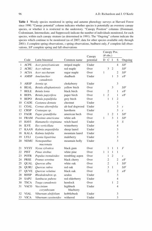
Table 1 Woody species monitored in spring and autumn phenology surveys at Harvard Forest since 1990. “Canopy potential” column indicates whether species is potentially an overstory canopy species, or whether it is restricted to the understory. “Canopy Position” columns (Dominant, Codominant, Intermediate, and Suppressed) indicate the number of individuals monitored, for each species, within each canopy stratum (as determined in 1991). The “Ongoing” column indicate the species which continue to be monitored (as of 2007; data for other species available only through 2001): S complete spring observations, s spring observations, budburst only, F complete fall obser-vations, S/F complete spring and fall observations
Canopy potential
Canopy Pos.(# obs.)
Code Latin binomial Common name D C I S Ongoing
1 ACPE Acer pensylvanicum striped maple Under 4 S/F 2 ACRU Acer rubrum red maple Over 3 2 S/F 3 ACSA Acer saccharum sugar maple Over 1 2 S/F 4 AMSP Amelanchier
canadensis shadbush Under 1 3 s/F
5 ARSP Aronia sp. chokeberry Under 3 6 BEAL Betula alleghaniensis yellow birch Over 3 S/F 7 BELE Betula lenta black birch Over 2 1 s/F 8 BEPA Betula papyrifera paper birch Over 1 2 1 s/F 9 BEPO Betula populifolia grey birch Over 1 1 2 10 CADE Castanea dentata chestnut Under 3 11 COAL Cornus alternifolia alt-leaf dogwood Under 3 s 12 CRSP Crataegus sp. hawthorn Under 3 s 13 FAGR Fagus grandifolia american bech Over 1 2 1 S/F 14 FRAM Fraxinus americana white ash Over 1 3 1 S/F 15 HAVI Hamamelis virginiana witch hazel Under 3 S 16 ILVE Ilex verticillata winterberry Under 4 17 KAAN Kalmia angustifolia sheep laurel Under 3 18 KALA Kalmia latifolia mountain laurel Under 3 19 LYLI Lyonia ligustrina maleberry Under 3 20 NEMU Nemopanthus
mucronata mountain holly Under 3
21 NYSY Nyssa sylvatica black gum Over 1 1 1 F 22 PIST Pinus strobus white pine Over 1 1 1 1 23 POTR Populus tremuloides trembling aspen Over 1 2 s 24 PRSE Prunus serotina black cherry Over 2 2 s/F 25 QUAL Quercus alba white oak Over 2 1 S/F 26 QURU Quercus rubra red oak Over 3 1 S/F 27 QUVE Quercus velutina black oak Over 2 2 s/F 28 RHSP Rhododendron sp. azalea Under 3 29 SAPU Sambucus pubens red elderberry Under 4 30 TSCA Tsuga canadensis hemlock Over 1 2 31 VACO Vaccinium
corymbosum highbush
blueberry Under 4
32 VIAL Viburnum alnifolium hobblebush Under 3 33 VICA Viburnum cassinoides witherod Under 3
Phenological Differences Between Understory and Overstory 97
black birch, paper birch, American beech, white ash, black gum, black cherry, white oak, red oak, and black oak). Our analysis here focuses on the years up to 2001, since the widest range of species are available for these years. However, when evaluating the complexity of budburst model structure that can be supported by the data, we conduct a separate analysis for the 17 species for which data since 2001 are also available.
Phenology observations are ongoing and the complete dataset is available online ( http://harvardforest.fas.harvard.edu/data/p00/hf003/hf003.html ).
Complete on-site climatological data are available for the period of study from the Shaler (1964–2002) and Fisher (2001−) meteorological stations, located near the forest’s administrative buildings. For this analysis, we use daily mean air tem-perature (°C), calculated from recorded daily maxima and minima.
2.3 Phenology Models
A variety of different models have been used to model spring phenology of temperate species (e.g., Hänninen 1995 ; Schwartz 1997 ; Chuine et al. 1998 ; Chuine 2000 ; Schaber and Badeck 2003 ; Richardson et al. 2006 ; note that models to predict autumn phenology are comparatively less-well developed, see Schaber and Badeck 2003) . To date, there is no consensus on which modeling approach is best. There are a number of reasons for this. First, models that give the best fit for one data set may perform the worst when validated against an external data set (Chuine et al. 1998, 1999) . Second, the model that works best for one species may perform poorly for other species (Hunter and Lechowicz 1992 ; Chuine et al. 1998, 1999) . Third, models that are considered physiologically realistic (see discussion by Hänninen 1995) have sometimes been found to perform no better than simple, empirical models (Hunter and Lechowicz 1992) . Fourth, a range of different model structures can often provide equally good fits to the available data (Hänninen 1995 ; Schaber and Badeck 2003) , and studies with synthetic data show that biologically “incorrect” models can be parameterized so as to provide good fits, and even to make satisfactory predictions (Hunter and Lechowicz 1992) .
Here we use the long-term Harvard Forest budburst and daily weather data to evaluate a range of models that have been previously presented in the literature. The models provide a context for interpreting observed differences in phenology among species and from year-to-year. A key question of interest is whether there are differ ences among species (particularly with regard to overstory vs. understory species) in terms of which model is best supported by the data at hand; from this it may be possible to learn about how species vary in relation to temperature sensitivi-ties and thresholds.
The models we use are largely based on (but not necessarily identical to) those presented by Chuine et al. (1999) , and our description and nomenclature follows this earlier work (see Table 2 for a list of symbols). Model parameters are fit separately for each species, allowing for species-specific biological responses to environmental cues; the parameters to be fit depend on the model structure (see Tables 2 and 3 ).
98 A.D. Richardson and J. O’Keefe
In general, budburst is predicted to occur only when some combination of chilling and accumulated warming (“forcing”) have been achieved (i.e., S
c ( t ) ³ C* and S
f ( t ) ³
F *). The state of chilling, S c , is the time integral (from t
1 ) of the rate of chilling, R
c ,
which is specified as a function of daily mean air temperature, x ( t ), i.e. Eqn. (1 ):
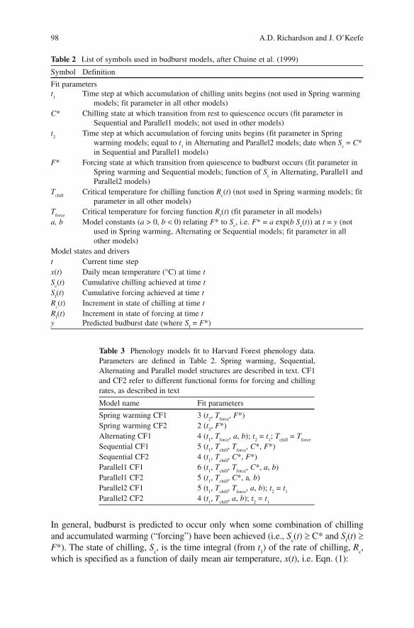
Table 2 List of symbols used in budburst models, after Chuine et al. (1999)
Symbol Definition
Fit parameters t 1 Time step at which accumulation of chilling units begins (not used in Spring warming
models; fit parameter in all other models) C * Chilling state at which transition from rest to quiescence occurs (fit parameter in
Sequential and Parallel1 models; not used in other models) t 2 Time step at which accumulation of forcing units begins (fit parameter in Spring
warming models; equal to t 1 in Alternating and Parallel2 models; date when S
c = C *
in Sequential and Parallel1 models) F * Forcing state at which transition from quiescence to budburst occurs (fit parameter in
Spring warming and Sequential models; function of S c in Alternating, Parallel1 and
Parallel2 models) T
chill Critical temperature for chilling function R
c ( t ) (not used in Spring warming models; fit
parameter in all other models) T
force Critical temperature for forcing function R
f ( t ) (fit parameter in all models)
a, b Model constants ( a > 0, b < 0) relating F * to S c , i.e. F * = a exp( b S
c ( t )) at t = y (not
used in Spring warming, Alternating or Sequential models; fit parameter in all other models)
Model states and drivers t Current time step x ( t ) Daily mean temperature (°C) at time t S
c ( t ) Cumulative chilling achieved at time t
S f ( t ) Cumulative forcing achieved at time t
R c ( t ) Increment in state of chilling at time t
R f ( t ) Increment in state of forcing at time t
y Predicted budburst date (where S f = F *)
Table 3 Phenology models fi t to Harvard Forest phenology data. Parameters are defi ned in Table 2 . Spring warming, Sequential, Alternating and Parallel model structures are described in text. CF1 and CF2 refer to different functional forms for forcing and chilling rates, as described in text
Model name Fit parameters
Spring warming CF1 3 ( t 2 , T
force , F *)
Spring warming CF2 2 ( t 2 , F *)
Alternating CF1 4 ( t 1 , T
force , a , b ); t
2 = t
1 ; T
chill = T
force
Sequential CF1 5 ( t 1 , T
chill , T
force , C *, F *)
Sequential CF2 4 ( t 1 , T
chill , C *, F *)
Parallel1 CF1 6 ( t 1 , T
chill , T
force , C *, a , b )
Parallel1 CF2 5 ( t 1 , T
chill , C *, a , b )
Parallel2 CF1 5 (t 1 , T
chill , T
force , a , b ); t
2 = t
1
Parallel2 CF2 4 ( t 1 , T
chill , a , b ); t
2 = t
1
Phenological Differences Between Understory and Overstory 99
1
c c( ) ( ( ))t
S t R x t= ∑ (1)
The cumulative state of forcing, S f , similarly represents the time integral (from t
2 ,
which, depending on model structure, either equals t 1 or requires that a chilling
thres hold be met, i.e. where S c ³ C *) of the rate of forcing, R
f , which is also a function
of air temperature, i.e. Eqn. ( 2 ):
2
f f( ) ( ( ))t
S t R x t= ∑ (2)
Models differ depending on whether or not a period of chilling is strictly required, either prior to or concurrently with forcing. In “spring warming” models (Cannell and Smith 1983 ; Hunter and Lechowicz 1992) , there are no chilling requirements and only forcing temperatures affect the timing of budburst. On the other hand, three types of chilling can be specified:
Sequential: In the sequential model, forcing has no effect until all chilling require-ments have been met. During a “period of rest”, the state of chilling accumulates from day t
1 until the state of chilling reaches a threshold value, C *. At this point (day t
2 )
there is a transition to a “period of quiescence” and accumulation of forcing units begins and continues until a threshold value, F *, is reached, triggering budburst.
Alternating: The state of chilling and the state of forcing both advance together over time from day t
1 (t
2 is set to t
1 ): above a threshold temperature, forcing degree-
days are accumulated; below the threshold temperature, chilling days are accumu-lated (thus forcing occurs whenever chilling is not occurring, and vice versa). Requirements for chilling and forcing thresholds C * and F * are not specified explicitly: rather, as more chilling is accumulated, the forcing required for budburst is reduced (when b < 0), here as in Eqn. ( 3 ):
( )* exp ( )cF a bS y= (3)
Parallel: Similar to the alternating model, in the parallel model forcing and chilling advance together over time, and as more chilling is accumulated, the forcing requirement for budburst is reduced. However, unlike the alternating model, forcing need not occur whenever chilling is not occurring. We distinguish two versions of parallel chilling. In the first (Parallel1), a threshold value of chilling, C *, must first be reached before forcing units are accumulated (i.e., the model requires a transition from rest to quiescence). In the second (Parallel2), chilling and forcing both accumulate from t
1 (i.e., t
2 is set to t
1 ). (Note that as described here, both sequential and alter-
nating chilling are essentially restricted versions of the parallel model. For more a more thorough treatment of chilling, see: Cannell and Smith 1983 ; Hunter and Lechowicz 1992 ; Kramer 1994 ; Chuine et al. 1998, 1999) .
For each of these different model structures (Spring warming, Sequential, Alternating or Parallel), various functional forms of the equations for R
c and R
f are
possible. Here we consider two variants. In one approach (here denoted CF1), the state of chilling is specified in terms of “chilling days,” which are accumulated as R
c = 1 where x(t) < T
chill and R
c = 0 otherwise, and the state of forcing is specified
100 A.D. Richardson and J. O’Keefe
in terms of “forcing degree-days,” which are accumulated as R f = x(t)-T
force where
x(t) > T force
and R f = 0 otherwise. In another approach (here denoted CF2), rates of
chilling and forcing are both specified as nonlinear functions of x(t) (Sarvas 1974 in Chuine et al. 1999). More specifically, in CF2, (unitless) chilling is accumulated according to the triangular function in Eqn. ( 4 ):
( ) ( )c 0 where 3.4 or 10.4R x t x t= ≤ − ≥ (4a)
( ) ( )c chillchill
3.4where 3.4
3.4
x tR x t T
T
+< ≤
+= − (4b)
( ) ( )c chill
chill
3.4where 10.4
10.4
x tR T x t
T
−= < ≤
− (4c)
In CF2, the rate of forcing is a sigmoid function of x ( t ), and (unitless) forcing is accumulated as in Eqn. ( 4 ) for x ( t ) > 0:
=+ − −f
28.4
1 exp( 0.185( ( ) 18.4))R
x t (5)
The way in which these submodels are combined, and the parameters that are optimized for each model, are listed in Table 3 . The resulting models vary both in complexity and in their underlying assumptions about the nature of the physiological processes involved, as manifest in terms of general model structure (e.g., the nature of chilling requirements and tradeoffs between S
c and F *), functional form (CF1 vs.
CF2), and the number of free parameters to be optimized.
2.4 Model Parameterization
Nonlinearities and discontinuities in phenology models (e.g., degree day accumula-tion begins on a particular day, above a particular temperature) mean there is a very real possibility of model parameter sets which yield only locally, and not globally, optimal agreement between model and data (e.g., Chuine et al. 1998) . Our parameter optimization method was based on simulated annealing-type routines using Monte Carlo techniques (Metropolis et al. 1953) as described by Press et al. (1992) and used previously to estimate phenology model parameters by Chuine et al. (1998) . FORTRAN code for the models and optimization algorithm is available from A.D.R.
2.5 Model Selection Criteria
An objective method is needed to select the most appropriate model from among a range of competing structures. While possible options include F -tests and within-sample or out-of-sample cross-validation methods, alternative approaches based on
Phenological Differences Between Understory and Overstory 101
information theory are becoming popular in many fields, including ecology. For example, Akaike’s (1973) criterion is rigorously based on the expected Kullback-Liebler information of each model (for a full overview of Akaike’s method, as well as many examples from the ecological literature, see Burnham and Anderson 2002) . Akaike’s Information Criterion (AIC) quantifies how well the data at hand support various candidate models. Assuming Gaussian errors with constant vari-ance, AIC is typically calculated as in Eqn. ( 6 ):
2AIC log( ) 2n ps= + (6)
Here, n is the number of observations, p is the number of fit parameters plus one, and s 2 is the residual sum of squares divided by n . The model with the lowest AIC is considered the best model, given the data at hand, but it is important to note that AIC is not in any sense a formal or statistical hypothesis test (Anderson et al. 2000) . For a given data set and a set of candidate models, AIC effectively balances improving explanatory power (lower s 2 ) against increasing complexity (larger p ). In this way, AIC selects against models with an excessive number of parameters.
Alternatives to AIC have been developed (e.g., Schwartz 1978 , Hurvich and Tsai 1990) , and while we will not discuss these here, we will apply a correction factor which has been developed for cases where n is small relative to p . The small-sample corrected criterion, AIC
C , is calculated (Burnham and Anderson 2002 ;
Motulsky and Christopoulos 2003) as in Eqn. ( 7 ):
C
2 ( 1)AIC AIC
1
p p
n p
+= +
− − (7)
The absolute difference in AIC C scores between two models can be used to evaluate
the weight of evidence in support of one model (the model with the lower AIC C ) over
another model (Burnham and Anderson 2002) : if the difference, D AIC C , is small or zero,
then both models are essentially equally likely to be the best model. If D AIC C » 2.0,
then the model with the lower AIC C is almost three times more likely to be best. If,
however, D AIC C » 6.0, then the model with the lower AIC
C is about 20 times more
likely to be best. Here we calculate D AIC C relative to the “best” model (lowest
AIC C ) for each species, and express all AIC-based results in terms of this metric.
3 Results
3.1 Patterns of Variation Among Species
For both canopy and understory species, budburst dates varied by roughly 6 weeks among species (Fig. 2 ; four-letter species codes are reported here in the text to facilitate figure interpretation; full species information is listed in Table 1 ). Among canopy species, black cherry (PRSE) had the earliest mean budburst date (day 110), while white pine (PIST) had the latest (day 157). Among understory species, red
102 A.D. Richardson and J. O’Keefe
elderberry (SAPU) had the earliest mean budburst date (day 105) and sheep laurel (KAAN) the latest (day 144). The date when leaves reached 75% of final size varied by a similar amount for canopy species (48 days, from day 134 for trembling aspen, POTR, to day 182 for white pine). However, the range of variation was only half as great for understory species (25 days, from day 141 for hobblebush, VIAL, to day 166 for mountain laurel, KALA).
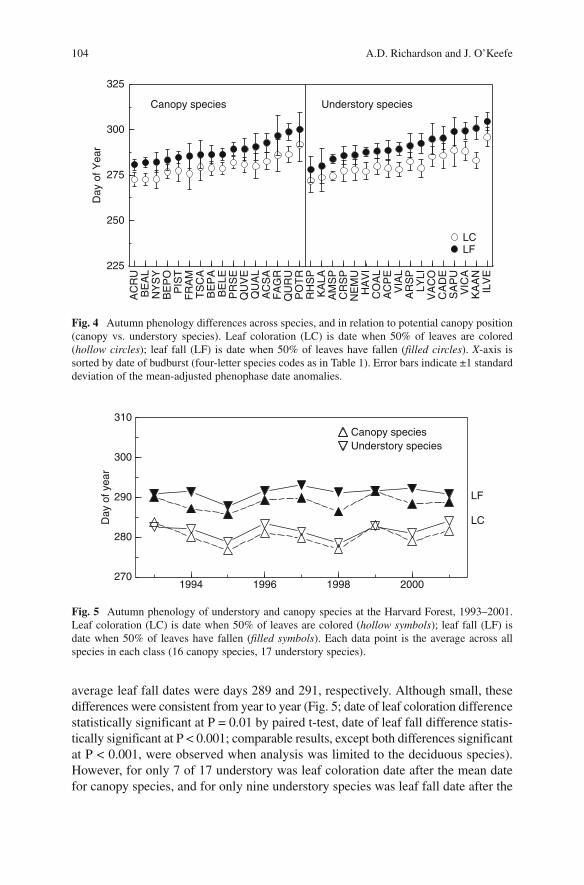
Fig. 2 Spring phenology differences across species, and in relation to potential canopy position (canopy vs. understory species). Budburst (BB) is date when 50% of leaf buds have burst ( hollow circles ); L75 is date when 50% of leaves have reached 75% of final size ( filled circles ). X -axis is sorted by date of budburst (four-letter species codes as in Table 1 ). Error bars indicate ±1 standard deviation of the mean-adjusted phenophase date anomalies.
100
125
150
175
200D
ay o
f Yea
r
BBL75
Canopy species Understory species
PR
SE
PO
TR
BE
PA
AC
SA
BE
AL
BE
PO
AC
RU
BE
LE
QU
RU
FR
AM
QU
VE
QU
AL
NY
SY
TS
CA
PIS
TS
AP
UV
ICA
VIA
LC
OA
LA
RS
PV
AC
OA
MS
PC
RS
PN
EM
UH
AV
IA
CP
EIL
VE
CA
DE
LYLI
RH
SP
KA
LAK
AA
N
FA
GR
Fig. 3 Spring phenology of understory and canopy species at the Harvard Forest, 1990–2001. Budburst (BB) is date when 50% of leaf buds have burst ( hollow symbols ); L75 is date when 50% of leaves have reached 75% of final size ( filled symbols ). Each data point is the average across all species in each class (16 canopy species, 17 understory species).
1990 1992 1994 1996 1998 2000100
120
140
160
180
Day
ofye
ar
Canopy speciesUnderstory species
L75
BB
Phenological Differences Between Understory and Overstory 103
The time required for leaf expansion (i.e., the number of days between budburst and when leaves reached 75% of final size) varied by roughly twofold. For canopy species, expansion took between 14 days (American beech, FAGR) and 32 days (black cherry), compared to between 18 days (azalea, RHSP) and 40 days (red elderberry) for understory species. For understory ( r = −0.67, P < 0.01), but not canopy ( r = 0.01, P = 0.97), species, the time required for expansion was negatively correlated with budburst date; in other words, leaf development progressed more slowly in early-leafing species than late-leafing species, which may be a result of degree-days accumulating more slowly in early spring compared to late spring.
There was a general tendency for budburst of understory species to be earlier than that of canopy species. In fact, budburst of 13 of 17 understory species occurred prior to the mean canopy budburst date. The only exceptions were the relatively late-leafing species maleberry, azalea, mountain laurel, and sheep laurel, two of which are ever-green species (mountain laurel and sheep laurel). The average budburst date for understory species was day 124, compared to day 130 for canopy species (day 120 and 126, respectively, when only deciduous species are considered). This pattern was consistent over time, with the difference always 3 days or greater (Fig. 3 ), and a paired (i.e., mean for understory species vs. mean for canopy species, paired by year) t -test indicated that this difference was statistically significant ( P < 0.001; results were unchanged when only deciduous species considered).
By comparison, the date when leaves reached 75% of final size differed little between canopy and understory species. The average date at which leaves reached this phenophase was day 150 for understory species, which was within a day of that for the canopy species. A t -test indicated no statistically significant difference between canopy and understory species ( P = 0.30; the same pattern was observed when analysis was limited to the deciduous species).
The date of leaf coloration varied by less than 3 weeks among canopy species, but by almost a full week more among understory species (Fig. 4 ). Among canopy species, red maple (ACRU) had the earliest mean leaf coloration date (day 274), while trembling aspen (POTR) the latest (day 292). Among understory species, azalea (RHSP) had the earliest mean leaf coloration date (day 272) while winter-berry (ILVE) had the latest (day 295). Thus both the earliest and latest species in terms of leaf coloration date tended to be understory species, although this was not the case in every year (e.g., POTR was in a number of years the latest species).
Whereas in the spring there was a strong tendency, particularly among understory species, to change rank order between budburst and when leaves reached 75% of final size (Fig. 2 ), in autumn the species order of leaf coloration and leaf fall was more consistent. For example, the earliest and latest species for leaf fall were the same as those for leaf coloration for both groups of species. Furthermore, the rank correlation between dates of leaf coloration and leaf fall was higher (Spearman rank correlation, ρ = 0.95) than between budburst date and the date when leaves reached 75% of final size ( ρ = 0.81).
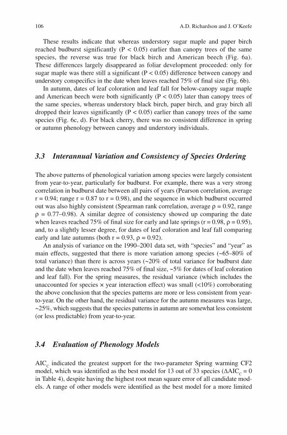
There was a slight tendency for dates of leaf coloration and leaf fall of understory species to be later than that of canopy species. The average leaf coloration date for canopy species was day 280, compared to day 281 for understory species; the
104 A.D. Richardson and J. O’Keefe
average leaf fall dates were days 289 and 291, respectively. Although small, these differences were consistent from year to year (Fig. 5 ; date of leaf coloration difference statistically significant at P = 0.01 by paired t-test, date of leaf fall difference statis-tically significant at P < 0.001; comparable results, except both differences significant at P < 0.001, were observed when analysis was limited to the deciduous species). However, for only 7 of 17 understory was leaf coloration date after the mean date for canopy species, and for only nine understory species was leaf fall date after the
Fig. 5 Autumn phenology of understory and canopy species at the Harvard Forest, 1993–2001. Leaf coloration (LC) is date when 50% of leaves are colored (hollow symbols); leaf fall (LF) is date when 50% of leaves have fallen ( filled symbols ). Each data point is the average across all species in each class (16 canopy species, 17 understory species).
1994 1996 1998 2000270
280
290
300
310
Day
of y
ear
Canopy speciesUnderstory species
LF
LC
Fig. 4 Autumn phenology differences across species, and in relation to potential canopy position (canopy vs. understory species). Leaf coloration (LC) is date when 50% of leaves are colored ( hollow circles); leaf fall (LF) is date when 50% of leaves have fallen ( filled circles ). X -axis is sorted by date of budburst (four-letter species codes as in Table 1 ). Error bars indicate ±1 standard deviation of the mean-adjusted phenophase date anomalies.
AC
RU
BE
AL
NY
SY
BE
PO
PIS
TF
RA
MT
SC
AB
EP
AB
ELE
PR
SE
QU
VE
QU
AL
AC
SA
FA
GR
QU
RU
PO
TR
RH
SP
KA
LAA
MS
PC
RS
PN
EM
UH
AV
IC
OA
LA
CP
EV
IAL
AR
SP
LYLI
VA
CO
CA
DE
SA
PU
VIC
AK
AA
NIL
VE
225
250
275
300
325D
ayof
Yea
r
LCLF
Canopy species Understory species

Phenological Differences Between Understory and Overstory 105
mean date for canopy species. Thus, while these patterns are statistically significant, they may not have great biological or ecological significance, and certainly do not indicate large differences in autumn phenology between broad groups of canopy and understory species. Rather, the differences are more pronounced among individual species within each group.
3.2 Differences Between Canopy and Conspecific Understory Trees
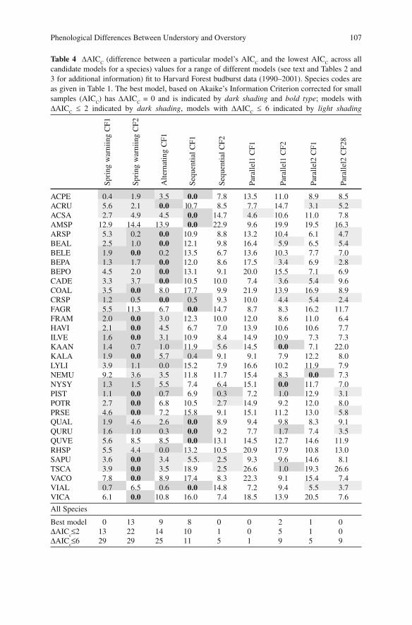
For six species (sugar maple, ACSA; black birch, BELE; paper birch, BEPA; gray birch, BEPO; American beech, FAGR; and black cherry, PRSE; see Table 1 ), one or more individuals of each was classified as either dominant or codominant (here, lumped together as “canopy trees”), and one or more individuals was classified as suppressed (here, “understory trees”). For each of these species we calculated, by year, the difference in date at which the canopy and understory trees reached each pheno-logical stage, and then conducted a simple two-tailed t -test on these differences.
AC
SA
BE
LE
BE
PA
BE
PO
FA
GR
PR
SE
AC
SA
BE
LE
BE
PA
BE
PO
FA
GR
PR
SE
−10
−5
0
5
10
−10
−5
0
5
10a
AC
SA
BE
LE
BE
PA
BE
PO
FA
GR
PR
SE
AC
SA
BE
LE
BE
PA
BE
PO
FA
GR
PR
SE
b
−30
−15
0
15
30
−30
−15
0
15
30c d
BB
dat
e
?
LC d
ate
?
L75
date
?
LF d
ate
?
Fig. 6 Difference in dates at which canopy and understory individuals of six species reach differ-ent phenophases at the Harvard Forest. Species are sugar maple (ACSA), black birch (BELE), paper birch (BEPA), gray birch (BEPO), American beech (FAGR) and black cherry (PRSE). A positive value indicates that canopy individuals reach that phenophase at a later date than under-story individuals. ( a ) Budburst (BB); ( b ) leaves reached 75% of final size (L75); ( c ) leaf coloration (LC); ( d ) leaf fall (LF). Error bars indicate 95% confidence intervals on the mean difference, with each year treated as a replicate.
106 A.D. Richardson and J. O’Keefe
These results indicate that whereas understory sugar maple and paper birch reached budburst significantly (P < 0.05) earlier than canopy trees of the same species, the reverse was true for black birch and American beech (Fig. 6a ). These differences largely disappeared as foliar development proceeded: only for sugar maple was there still a significant (P < 0.05) difference between canopy and understory conspecifics in the date when leaves reached 75% of final size (Fig. 6b ).
In autumn, dates of leaf coloration and leaf fall for below-canopy sugar maple and American beech were both significantly (P < 0.05) later than canopy trees of the same species, whereas understory black birch, paper birch, and gray birch all dropped their leaves significantly (P < 0.05) earlier than canopy trees of the same species (Fig. 6c , d ). For black cherry, there was no consistent difference in spring or autumn phenology between canopy and understory individuals.
3.3 Interannual Variation and Consistency of Species Ordering
The above patterns of phenological variation among species were largely consistent from year-to-year, particularly for budburst. For example, there was a very strong correlation in budburst date between all pairs of years (Pearson correlation, average r = 0.94; range r = 0.87 to r = 0.98), and the sequence in which budburst occurred out was also highly consistent (Spearman rank correlation, average ρ = 0.92, range ρ = 0.77–0.98). A similar degree of consistency showed up comparing the date when leaves reached 75% of final size for early and late springs (r = 0.98, ρ = 0.95), and, to a slightly lesser degree, for dates of leaf coloration and leaf fall comparing early and late autumns (both r = 0.93, ρ = 0.92).
An analysis of variance on the 1990–2001 data set, with “species” and “year” as main effects, suggested that there is more variation among species ( ~ 65–80% of total variance) than there is across years ( ~ 20% of total variance for budburst date and the date when leaves reached 75% of final size, ~ 5% for dates of leaf coloration and leaf fall). For the spring measures, the residual variance (which includes the unaccounted for species × year interaction effect) was small (<10%) corroborating the above conclusion that the species patterns are more or less consistent from year-to-year. On the other hand, the residual variance for the autumn measures was large, ~ 25%, which suggests that the species patterns in autumn are somewhat less consistent (or less predictable) from year-to-year.
3.4 Evaluation of Phenology Models
AIC C indicated the greatest support for the two-parameter Spring warming CF2
model, which was identified as the best model for 13 out of 33 species ( D AIC C = 0
in Table 4 ), despite having the highest root mean square error of all candidate mod-els. A range of other models were identified as the best model for a more limited
Phenological Differences Between Understory and Overstory 107
Table 4 D AIC C (difference between a particular model’s AIC
C and the lowest AIC
C across all
candidate models for a species) values for a range of different models (see text and Tables 2 and 3 for additional information) fi t to Harvard Forest budburst data (1990–2001). Species codes are as given in Table 1 . The best model, based on Akaike’s Information Criterion corrected for small samples (AIC
C ) has D AIC
C = 0 and is indicated by dark shading and bold type ; models with
D AIC C £ 2 indicated by dark shading , models with D AIC
C £ 6 indicated by light shading
Spri
ng w
arni
ing
CF1
Spri
ng w
arni
ing
CF2
Alte
rnat
ing
CF1
Sequ
entia
l CF1
Sequ
entia
l CF2
Para
llel1
CF1
Para
llel1
CF2
Para
llel2
CF1
Para
llel2
CF2
8
ACPE 0.4 1.9 3.5 0.0 7.8 13.5 11.0 8.9 8.5 ACRU 5.6 2.1 0.0 l0.7 8.5 7.7 14.7 3.1 5.2 ACSA 2.7 4.9 4.5 0.0 14.7 4.6 10.6 11.0 7.8 AMSP 12.9 14.4 13.9 0.0 22.9 9.6 19.9 19.5 16.3 ARSP 5.3 0.2 0.0 10.9 8.8 13.2 10.4 6.1 4.7 BEAL 2.5 1.0 0.0 12.1 9.8 16.4 5.9 6.5 5.4 BELE 1.9 0.0 0.2 13.5 6.7 13.6 10.3 7.7 7.0 BEPA 1.3 1.7 0.0 12.0 8.6 17.5 3.4 6.9 2.8 BEPO 4.5 2.0 0.0 13.1 9.1 20.0 15.5 7.1 6.9 CADE 3.3 3.7 0.0 10.5 10.0 7.4 3.6 5.4 9.6 COAL 3.5 0.0 8.0 17.7 9.9 21.9 13.9 16.9 8.9 CRSP 1.2 0.5 0.0 0.5 9.3 10.0 4.4 5.4 2.4 FAGR 5.5 11.3 6.7 0.0 14.7 8.7 8.3 16.2 11.7 FRAM 2.0 0.0 3.0 12.3 10.0 12.0 8.6 11.0 6.4 HAVI 2.1 0.0 4.5 6.7 7.0 13.9 10.6 10.6 7.7 ILVE 1.6 0.0 3.1 10.9 8.4 14.9 10.9 7.3 7.3 KAAN 1.4 0.7 1.0 11.9 5.6 14.5 0.0 7.1 22.0 KALA 1.9 0.0 5.7 0.4 9.1 9.1 7.9 12.2 8.0 LYLI 3.9 1.1 0.0 15.2 7.9 16.6 10.2 11.9 7.9 NEMU 9.2 3.6 3.5 11.8 11.7 15.4 8.3 0.0 7.3 NYSY 1.3 1.5 5.5 7.4 6.4 15.1 0.0 11.7 7.0 PIST 1.1 0.0 0.7 6.9 0.3 7.2 1.0 12.9 3.1 POTR 2.7 0.0 6.8 10.5 2.7 14.9 9.2 12.0 8.0 PRSE 4.6 0.0 7.2 15.8 9.1 15.1 11.2 13.0 5.8 QUAL 1.9 4.6 2.6 0.0 8.9 9.4 9.8 8.3 9.1 QURU 1.6 1.0 0.3 0.0 9.2 7.7 1.7 7.4 3.5 QUVE 5.6 8.5 8.5 0.0 13.1 14.5 12.7 14.6 11.9 RHSP 5.5 4.4 0.0 13.2 10.5 20.9 17.9 10.8 13.0 SAPU 3.6 0.0 3.4 5.5. 2.5 9.3 9.6 14.6 8.1 TSCA 3.9 0.0 3.5 18.9 2.5 26.6 1.0 19.3 26.6 VACO 7.8 0.0 8.9 17.4 8.3 22.3 9.1 15.4 7.4 VIAL 0.7 6.5 0.6 0.0 14.8 7.2 9.4 5.5 3.7 VICA 6.1 0.0 10.8 16.0 7.4 18.5 13.9 20.5 7.6
All Species
Best model 0 13 9 8 0 0 2 1 0 ΔAIC
c ≤ 2 13 22 14 10 1 0 5 1 0
ΔAIC c ≤ 6 29 29 25 11 5 1 9 5 9
108 A.D. Richardson and J. O’Keefe
number of species: for example, the Alternating CF1 and Sequential CF1 models were indicated to be the best model for eight and nine species, respectively. However, the most highly parameterized model, Parallel1 CF1, with six parameters and the lowest RMSE, was not identified by AIC
C to be the best model for any of
the 33 species. Simply put, with time series of only 12 years in length, a model with six parameters cannot be justified, because the penalty associated with additional parameters is larger than the associated improvement in model fit (even with 17 years of data, a model with five parameters would have to fit the data twice as well as a model with two parameters for the models to have the same AIC
C value).
Models with D AIC C less than 2 are still considered to be reasonably well-
supported by the data (Burnham and Anderson 2002) . For the Spring warming CF2 model, D AIC
C was £ 2 for 22 species (and £ 6, which might be considered the limit
at which a claim could be made that the data give any support for the model, for 29 species) (Table 4 ). No other model had D AIC
C £ 2 for more than 14 species; but the
Spring warming CF1 and Alternating CF1 models both had D AIC C £ 6 for more
than three quarters of all species. These patterns did not differ markedly between canopy and understory species;
in both instances, the Spring warming CF2 model was identified as the best model for at least six species, and the patterns of variation in support for other models was comparable for both groups of species (summary results not shown). There was no obvious relationship between the timing of budburst (i.e., early vs. late leafing species) and the way in which models were ranked by AIC
C .
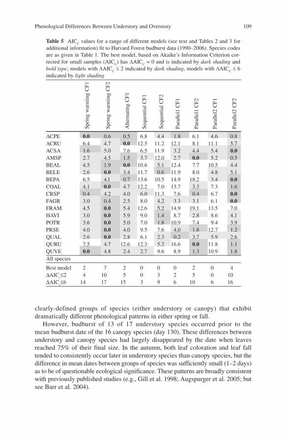
For the subset of species for which budburst observations have continued since 2001, we conducted a similar analysis on the 17-year data set (1990–2006) to inves-tigate whether additional model complexity could be justified if longer time series were used for model fitting. Again, the Spring warming CF2 model had the lowest AIC
C for the largest number of species (7 of 17), and the Spring warming CF1 and
Alternating CF1 models were at least marginally supported by the data for most species (Table 5 ). However, the five-parameter Parallel1 CF2 model and, to an even greater degree, the four-parameter Parallel2 CF2 model ( D AIC
C £ 2 for 10 of 17 species), both
emerged as viable candidate models in this analysis. This anaysis indicated greater support for the CF2, compared to CF1, formulations for rates of chilling and forcing: for the Spring warming, Sequential, Parallel1 and Parallel2 models, AIC
C values
were consistently (75% of all species, on average) lower for CF2 than CF1 versions.
4 Discussion
4.1 Do Canopy and Understory Species Differ Phenologically?
The Harvard Forest phenology data show (Figs. 2 and 4 ) that in both spring and fall, there is a continuum of phenological activity, from “early” to “late” species. Interestingly, the range of variation is not markedly different for understory and canopy species. Moreover, on the surface, we do not see strong evidence of any
Phenological Differences Between Understory and Overstory 109
clearly-defined groups of species (either understory or canopy) that exhibit dramatically different phenological patterns in either spring or fall.
However, budburst of 13 of 17 understory species occurred prior to the mean budburst date of the 16 canopy species (day 130). These differences between understory and canopy species had largely disappeared by the date when leaves reached 75% of their final size. In the autumn, both leaf coloration and leaf fall tended to consistently occur later in understory species than canopy species, but the difference in mean dates between groups of species was sufficiently small (1–2 days) as to be of questionable ecological significance. These patterns are broadly consistent with previously published studies (e.g., Gill et al. 1998 ; Augspurger et al. 2005 ; but see Barr et al. 2004) .
Table 5 AIC C values for a range of different models (see text and Tables 2 and 3 for
additional information) fi t to Harvard Forest budburst data (1990–2006). Species codes are as given in Table 1 . The best model, based on Akaike’s Information Criterion cor-rected for small samples (AIC
C ) has D AIC
C = 0 and is indicated by dark shading and
bold type ; models with D AIC C £ 2 indicated by dark shading , models with D AIC
C £ 6
indicated by light shading
Spri
ng w
arni
ing
CF1
Spri
ng w
arni
ing
CF2
Alte
rnat
ing
CF1
Sequ
entia
l CF1
Sequ
entia
l CF2
Para
llel1
CF1
Para
llel1
CF2
Para
llel2
CF1
Para
llel2
CF2
ACPE 0.0 0.6 0.5 6.8 4.4 1.8 6.1 4.6 0.8 ACRU 6.4 4.7 0.0 12.5 11.2 12.1 8.1 11.1 5.7 ACSA 1.6 5.0 7.6 6.5 11.9 3.2 4.4 5.4 0.0 AMSP 2.7 4.5 1.5 3.7 12.0 2.7 0.0 5.2 0.5 BEAL 4.5 1.9 0.0 10.6 5.1 12.4 7.7 10.5 4.4 BELE 2.6 0.0 3.4 11.7 0.6 11.9 8.0 4.8 5.1 BEPA 6.5 4.l 0.7 13.6 10.5 14.9 18.2 3.4 0.0 COAL 4.1 0.0 4.7 12.2 7.0 13.7 3.3 7.3 1.6 CRSP 0.4 4.2 4.0 6.0 11.3 7.6 0.4 6.7 0.0 FAGR 3.0 0.4 2.5 8.0 4.2 3.3 3.1 6.1 0.0 FRAM 4.5 0.0 5.4 12.6 5.2 14.9 19.1 13.5 7.0 HAVI 3.0 0.0 5.9 9.0 1.4 8.7 2.8 8.6 4.1 POTR 3.6 0.0 5.0 7.0 1.8 10.9 7.4 9.4 3.9 PRSE 4.0 0.0 4.0 9.5 7.6 4.0 1.8 12.7 1.2 QUAL 2.6 0.0 2.8 6.1 2.3 0.2 3.7 5.9 2.6 QURU 7.5 4.7 12.6 12.3 5.2 16.6 0.0 11.8 1.1 QUVE 0.0 4.8 2.4 2.7 9.6 8.9 1.3 10.9 1.8 All species
Best model 2 7 2 0 0 0 2 0 4 ΔAIC
c ≤ 2 4 10 5 0 3 2 5 0 10
ΔAIC c ≤ 6 14 17 15 3 9 6 10 6 16
110 A.D. Richardson and J. O’Keefe
In 10 of 17 understory species, budburst occurred prior to day 125 (species SAPU, red elderberry, through HAVI, witch hazel, in Fig. 2 ), whereas none of the five most dominant canopy species reach budburst until this date (yellow birch is the first, on day 125; but the most abundant species, red oak, does not reach bud-burst until day 129). Thus, these ten species are candidates for being classified as having adopted strategies of springtime phenological escape – but clearly the suc-cess with which this strategy is adopted (in terms of the potential increases in light interception and photosynthetic assimilation) varies among species, with the ben-efit potentially being considerably larger to the earliest species, such as red elder-berry, compared to late budburst species, such as witch hazel. As noted above, however, the realized gains depend on the rate at which photosynthetic capacity is developed following leaf-out, and note that understory species tended to progress more slowly from budburst to 75% of final size, which could imply slow develop-ment of photosynthetic capacity as well.
Three understory species (striped maple, winterberry, and chestnut) leaf out between day 125 and day 130, i.e. concurrently with the majority of canopy spe-cies, and appear not to rely on the escape strategy. Special mention should be made of striped maple, which is known to be extremely shade tolerant, and chestnut, which was a dominant overstory tree across much of the eastern United States until the arrival of the chestnut blight in the early 1900s. Chestnut is now essentially restricted to root-sprouted saplings and small trees in the forest understory. It could be argued that chestnut would more appropriately be classified as a canopy species, but this would not change our overall interpretation of the patterns reported here.
Two of the four understory species with especially late budburst, mountain laurel (KALA) and sheep laurel (KAAN), are evergreen species that would presumably benefit little from early budburst or delayed senescence, since they retain most of their foliage throughout the entire year. In this manner, evergreen understory species are still able to exploit the spring and autumn high-light periods, and photosynthesis at these times of the year is considered important for their survival (e.g., Lassoie et al. 1983) . Interestingly, while these species are both characterized by late budburst in spring, they are among the earliest (e.g., mountain laurel) and latest (sheep laurel) species to drop their leaves in autumn (Fig. 4 ).
In the autumn, the single most abundant species, red oak (QURU, accounting for 36% of basal area), is the third-last species to drop its leaves in this community (Fig. 4 ), which would make an autumn strategy of phenological escape relatively difficult for most understory species. On the other hand, red maple (ACRU) and yellow birch (BEAL) are both among the five most dominant canopy species but drop their leaves very early (Fig. 4 ). These examples highlight the fact that during the spring and autumn transition periods, the developmental state of the canopy is highly variable across space. Thus the amount of light reaching any point in the understory depends on the phenology of neighboring species (Kato and Komiyama 2002) . In this regard, the degree to which an individual plant in the understory is able to opportunistically take advantage of spring and autumn high light periods largely depends on the species under which that plant grows. Detailed measure-ments to quantify the light environment experienced by individual understory
Phenological Differences Between Understory and Overstory 111
plants, e.g., vertical profiles of leaf area index and clumping indices (and how these, and thus f
TPAR, vary seasonally), would offer insights into the degree to which
a strategy of phenological escape is being successfully adopted. Previous studies comparing phenology of understory and canopy species (e.g.
Gill et al. 1998 , Augspurger et al. 2005) have limited their analysis to a more restricted set of species than was considered here; our survey gives a broad overall view of phenological patterns within a forest community. We see that in springtime, there is a loosely-defined subset of understory species that appear to adopt a strategy of phenological escape; most of the non-evergreen species followed this strategy to some degree. However, the difference between understory and canopy species at Harvard Forest appears to be smaller than has been reported in previous studies. For example, only two understory species, red elderberry and witherod (SAPU and VICA in Fig. 2 ), had budburst that was more than 10 days in advance of budburst by any of the dominant canopy species. For the remaining 11 species that tended to leaf out in advance of the mean canopy budburst date, the period of phenological escape was generally very short, only on the order of several days, and thus the functional significance of the strategy (and the role of phenological escape in struc-turing the community) is not clear. This is a surprising result because it suggests that the costs (or associated risks) of earlier emergence at Harvard Forest may be larger than in other ecosystems where similar research has been previously conducted.
There are even less pronounced differences between canopy and understory species in the autumn. Both competitive and abiotic factors could explain this. For example, because the most dominant canopy species, red oak, is among the latest to drop its leaves, much of the understory remains shaded until very late autumn, by which time cooler temperatures, shorter days, and lower peak irradiances substantially reduce the potential photosynthetic gains of autumn phenological escape.
4.2 Do Canopy and Understory Conspecifics Differ Phenologically?
Previous studies have provided relatively consistent evidence of earlier budburst, but not necessarily later abscission, by understory individuals of canopy species (e.g., Augspurger and Bartlett 2003) . Here, our evaluation of phenological differ-ences between canopy trees and understory individuals of the same species indi-cates surprisingly mixed results in both spring and fall. For example, in spring, understory individuals of sugar maple and paper birch tended to reach budburst significantly earlier (by more than 5 days in the case of sugar maple) than canopy individuals, whereas the reverse was true for yellow birch and American beech (Fig. 6a ). The pattern for sugar maple and paper birch is consistent with what would be expected based on previous studies, which generally show that within a species, seedlings, saplings and small trees leaf out in advance of mature canopy trees (Gill et al. 1998 ; Seiwa 1999a, b ; Augspurger and Bartlett 2003) , presumably because the potential carbon gains from earlier budburst decrease with increasing height.
112 A.D. Richardson and J. O’Keefe
The pattern for yellow birch and American beech is counter-intuitive, as this did not occur in any of the 13 species studied by Augspurger and Bartlett (2003) , and Gill et al. (1998) reported exactly the opposite for American beech growing in a north-ern hardwood forest. The fact that differences between understory and canopy individuals had largely disappeared by the date when leaves reached 75% of final size (Fig. 6b ) is surprising, as Augspurger and Bartlett (2003) reported that full leaf expansion also tended to occur earlier in juveniles than adults.
In autumn, leaf coloration and leaf fall of sugar maple and American beech understory individuals was much later (20 days in the case of American beech) than canopy individuals (comparable to patterns reported for these same species by Gill et al. 1998) , whereas smaller but significant differences in the opposite direction were seen for paper birch (Fig. 6c , d ). Similarly mixed results have been reported previously in the literature for autumn phenology (Seiwa 1999a, b ; Augspurger and Bartlett 2003) .
Within species, phenological differences between understory and canopy indi-viduals have been attributed to vertical temperature gradients, with warmer ground-level temperatures in spring promoting earlier emergence (Gill et al. 1998 ; Augspurger 2004) . If spring phenology is indeed under environmental, rather than developmental, control (Augspurger 2004) , then these apparently species-specific patterns in the Harvard Forest data may be the result of microclimatic differences among understory individuals due to variation in topography (Fisher et al. 2006) , canopy openness (Augspurger and Bartlett 2003) , or even the phenology of neigh-boring species.
4.3 Do Species Respond Differently to Climatic Variation?
Our results indicated that the ordering of species in terms of phenological sequence was relatively consistent in spring (i.e., for budburst date and the date when leaves reached 75% of final size; see also Lechowicz 1984) from year-to-year, but somewhat less so in autumn (i.e., for dates of leaf coloration and leaf fall). This may be partially attributed to inherent uncertainties in the autumn measures, which are considerably more subjective than well-defined phenophases, such as budburst. The difference in consistency between spring and autumn ordering may also be a function of differences in species-level responses to environmental signals. For example, we might hypothesize that whereas all species are responding to similar temperature cues in the springtime, in autumn some species might be responding to various temperature thresholds, whereas other species are responding to changes in day length. In addition, drought, as well as wind and rain (major autumn storms tend to bring down a large number of leaves), are factors that affect autumn senescence and abscission, but possibly result in more stochastic and less predictable patterns of autumn phenology.
Akaike’s Information Criterion indicated that the support for different pheno-logical model structures was mixed and varied somewhat among species (Table 4 ). Although there was no clear consensus model that consistently worked best (see
Phenological Differences Between Understory and Overstory 113
also Chuine et al. 1998) for all 33 study species (1990–2001 data), the data for most species gave reasonably strong support for three models, with the Spring warming CF2 model clearly the top choice. Both Hunter and Lechowicz (1992) and Chuine et al. (1998, 1999) also reported that a spring warming model performed as well, if not better than, more complex models involving chilling requirements. However, whereas results of Hunter and Lechowicz (1992) indicated support for a model with sequential chilling but not parallel chilling, results of Chuine et al. (1998) indicate support for a model with alternating chilling but not sequential or parallel chilling. Our results were mixed, differing depending on whether the shorter 1990–2001 (33 species) or longer 1990–2006 (17 species) dataset was being analyzed: the Sequential CF1 model was well-supported by 14 of 33 species in the shorter data set, but none of the 17 species in the longer data set, whereas the Parallel2 CF2 model was well supported by none of 33 species in the shorter data set, but 10 of 17 species in the longer data set. A possible explanation for this unusual pattern is that climatic conditions (and the phenological response to those conditions) for one or more years between 2002 and 2006 may have been sufficiently different from those between 1990 and 2001 to be incompatible with the Sequential CF1 model. However, as noted by Hänninen (1995) , rigorous testing of mechanistic phenology models of the type studied here really requires experimental, rather than observa-tional, data sets.
We saw no evidence of differences between overstory and understory species, or between evergreen and deciduous species, in terms of which model structure was preferred. And, while Schaber and Badeck (2003) reported that the best-fitting models differed between species with early and late budburst dates in Germany, we did not see evidence of a similar pattern in the Harvard Forest data. A possible explanation for this difference is that none of our models explicitly accounted for photoperiod (although, in spring warming models, the date at which forcing starts to accumulate could be interpreted as a photoperiod cue), whereas Schaber and Badeck (2003) found that day length improved model performance for species with late budburst (but see Cannell and Smith 1983) .
Because similar model structures were indicated for most species, it could be difficult to argue that phenological responses are driven by species-specific cues (cf. Schaber and Badeck 2003) . For example, there was no evidence that one group of species required sequential chilling, while another required parallel chilling, while a third group responded just to spring warming. On the other hand, looking at the species-specific model parameterization, certain species stand out as occupy-ing distinct regions of multivariate parameter space. For example, for the Spring warming CF2 model, the understory evergreen species sheep laurel and mountain laurel, although late leafing, did not appear to require more forcing than other species, but rather appeared insensitive to forcing until early May, whereas many other species respond to forcing beginning in late March. For the Parallel2 CF2 model, there were large and significant differences among species in the parameters a and b, which control the degree to which the accumulated chilling reduces the forcing requirement (strongly in some species, almost not at all in other species). Similarly, the optimal chilling temperature, and the date at which chilling begins to accumu-
114 A.D. Richardson and J. O’Keefe
late, varied substantially among species. These differences in parameterization give insights into biologically-based species-specific responses to the environment (Hunter and Lechowicz 1992) , and thus why the sequence in which budburst occurs might vary slightly from year-to-year. Furthermore, in the context of climate change, these differences have implications for how species will respond to future climates (Murray et al. 1989 ; Kramer 1994 ; see also Chuine et al. 2000 for an historical analysis), and thus imply that changes in the order that species leaf out can be expected. As evidence of this, we note that the species ordering was largely consistent between “early” and “late” spring years (Spearman rank correlation, P = 0.98), but whereas budburst of gray birch was more than 9 days earlier in “early” spring years, for hemlock it was only 3 days earlier. Although Kramer (1994) reported that species with late-spring budburst tend to exhibit less interannual variation (and thus less sensitivity to climatic variation) than those that leaf out in early spring (see also Murray et al. 1989), our results give only weak support for this hypothesis in general. The correlation between mean (by species) budburst date and the stand-ard deviation (by species, across years) of budburst dates was in the expected direc-tion (negative) but significantly different from zero only for understory ( r = −0.54, P = 0.02) species. For canopy ( r = 0.10, P = 0.72) species, or all species together ( r = −0.14, P = 0.44), the correlation was not significantly different from zero.
5 Summary and Conclusions
We conducted an analysis of the long term Harvard Forest phenology record to investigate differences in spring and autumn phenology both among (understory species vs. canopy species) and within species (understory vs. canopy conspecifics). Budburst of most understory species occurred prior to budburst by any of the dominant canopy species, suggesting a strategy of phenological escape, although the period of escape was limited to just a few days for most understory species. Phenological differences between understory and canopy species had largely disap-peared by the time leaves approached full expansion. Furthermore, in autumn, dif-ferences between understory and canopy species were less clear-cut; late abscission by the dominant canopy species, red oak, would tend to make phenological escape in this community a less viable strategy in autumn than in spring. Comparing understory and conspecific canopy individuals, we found that the patterns depended on the species in question: both earlier and later budburst, and accelerated or delayed senescence, were observed. An evaluation of a range of different models to predict budburst indicated support for both Spring warming models, with no chilling requirement, as well as models featuring Alternating and Parallel chilling. Models with Sequential chilling were not supported by the data. Although these patterns were broadly consistent among species, analysis of model parameterization indicated some differences in how species respond to environmental forcing. These differences help to explain the small year-to-year differences observed in the sequence of budburst among species.
Phenological Differences Between Understory and Overstory 115
This study, particularly the contrasting patterns of support for different models depending on whether the shorter (12 year) 33-species dataset or the longer (17 year) 17-species dataset was used, highlights the value of long-term, multi-species phenological data sets, with which it is possible to ask both ecological (how does phenology vary among and within species?) and biological (what environmental cues drive phenological events such as budburst?) questions. With ongoing efforts to link diverse “types” of phenology – e.g., to understand connections between phenology of above- (e.g., leaves) and below-ground (e.g., roots) growth, develop-ment and senescence, and how these relate to the phenology of ecosystem processes (particularly those related to the biogeochemical cycling of carbon and mineral nutrients, as discussed in many of the papers in this volume) as well as feedbacks to the climate system (surface albedo and partitioning of available energy to latent and sensible heat; Morisette et al. 2009) – mechanistic understanding of the causes of phenological differences both within and among species is of critical impor-tance. Evidence documenting phenological changes in response to recent warming trends (Schwartz et al. 2006) suggests that the value of these long-term monitoring data will only continue to increase over time (Lovett et al. 2007) .
Acknowledgements The National Science Foundation Long-Term Ecological Research (LTER) program supported the research at Harvard Forest. A.D.R. acknowledges support from the Northeastern States Research Cooperative. We thank Jeremy Fisher, Brenden McNeil, Alan Barr, Abraham Miller-Rushing, Jake Weltzin, and Asko Noormets for helpful comments on drafts of this chapter. This is a contribution of the Northeast Regional Phenology Network (NE-RPN).
References
Akaike , H. (1973) Information theory and an extension of the maximum likelihood principle . In: B.N. Petrov and F. Csaki (Eds.), Proceedings of the 2nd International Symposium on Information Theory , Akademiai Kiado , Budapest , pp. 267 – 281 . (Reproduced in: S. Kotz and N.L. Johnson (2003), Breakthroughs in Statistics, Vol. I, Foundations and Basic Theory . Springer, New York, pp. 610–624.)
Anderson , D.R. , Burnham , K.P. and Thompson , W.L. (2000) Null hypothesis testing: problems, prevalance and an alternative . J. Wildlife Manage. 64 , 912 – 923 .
Augspurger , C.K. (2004) Developmental versus environmental control of early leaf phenology in juvenile Ohio buckeye (Aesculus glabra) . Can. J. Bot. 82 , 31 – 36 .
Augspurger , C.K. and Bartlett , E.A. (2003) Differnces in leaf phenology between juvenile and adult trees in a temperate deciduous forest . Tree Physiol. 23 , 517 – 525 .
Augspurger , C.K. , Cheeseman , J.M. and Salk , C.F. (2005) Light gains and physiological capacity of understorey woody plants during phenological avoidance of canopy shade . Funct. Ecol. 19 , 537 – 547 .
Baldocchi , D. , Hutchison , B. , Matt , D. and McMillen , R. (1984) Seasonal variations in the radia-tion regime within an oak-hickory forest . Agric. For. Meteorol. 33 , 177 – 191 .
Baldochi , D. , Hutchison , B. , Matt , D. and McMillen , R. (1986) Seasonal variation in the statistics of photosynthetically active radiation penetration in an oak-hickory forest . Agric. For. Meteorol. 36 , 343 – 361 .
Barr , A.G. , Black , T.A. , Hogg , E.H. , Kljun , N. , Morgenstern , K. and Nesic , Z. (2004) Inter-annual variability in the leaf area index of a boreal aspen-hazelnut forest in relation to net ecosystem production . Agric. For. Meteorol. 126 , 237 – 255 .
116 A.D. Richardson and J. O’Keefe
Boardman , N.K. (1977) Comparative photosynthesis of sun and shade plants . Ann. Rev. Plant Physiol. 28 , 355 – 377 .
Burnham , K.P. and Anderson , D.R. (2002) Model selection and multimodel inference: a practical information-theoretic approach ( 2nd ed. ). Springer , New York .
Cannell , M. and Smith , R. (1983) Thermal time, chill days and prediction of budburst in Picea sitchensis . J. Appl. Ecol. 20 , 951 – 963 .
Chazdon , R.L. and Pearcy , R.W. (1991) The importance of sunflecks for forest understory plants . BioScience 41 , 760 – 766 .
Chen , W.J. , Black , T.A. , Yang , P.C. , Barr , A.G. , Neumann , H.H. , Nesic , Z. , Blanken , P.D. , Novak , M.D. , Eley , J. , Ketler , R.J. and Cuenca , R. (1999) Effects of climatic variability on the annual carbon sequestration by a boreal aspen forest . Global Change Biol. 5 , 41 – 53 .
Chuine , I. (2000) A unified model for budburst of trees . J. of Theor. Biol. 207 , 337 – 347 . Chuine, I., Cambon, G. and Comtois, P. (2000) Scaling phenology from the local to the regional
level: advances from species-specific phenological models. Global Change Biol. 6, 943–952. Chuine , I. , Cour , P. and Rousseau , D.D. (1998) Fitting models predicting dates of flowering of
temperate-zone trees using simulated annealing . Plant Cell Environ. 21 , 455 – 466 . Chuine , I. , Cour , P. and Rousseau , D.D. (1999) Selecting models to predict the timing of flowering
of temperate trees: implications for tree phenology modelling . Plant Cell Environ. 22 , 1 – 13 . Crawley , M.J. (1997) Life history and environment . In: M.J. Crawley (Ed.) Plant Ecology .
Blackwell Science , Oxford , pp. 73 – 131 . dePamphilis , C.W. and Neufeld , H.S. (1989) Phenology and ecophysiology of Aesculus sylvatica,
a vernal understory tree . Can. J. Bot. 67 , 2161 – 2167 . Fisher , J.I. , Mustard , J.F. and Vadeboncoeur , M.A. (2006) Green leaf phenology at Landsat resolu-
tion: Scaling from the field to the satellite . Remote Sens. Environ. 100 , 265 – 279 . Fisher , J.I. , Richardson , A.D. and Mustard , J.F. (2007) Phenology model from surface meteorol-
ogy does not capture satellite-based greenup estimations . Global Change Biol. 13 , 707 – 721 . Gill , D.S. , Amthor , J.S. and Bormann , F.H. (1998) Leaf phenology, photosynthesis, and the persist-
ence of saplings and shrubs in a mature northern hardwood forest . Tree Physiol. 18 , 281 – 289 . Gu , L. , Hanson , P.J. , Post , W.M. , Kaiser , D.P. , Yang , B. , Nemani , R. , Pallardy , S.G. , Meyers , T. ,
2008 . The 2007 eastern US spring freeze: Increased cold damage in a warming world? BioScience , 58 , 253 – 262 .
Hänninen , H. (1995) Effects of climatic change on trees from cool and temperate regions: an ecophysiological approach to modeling of bud burst phenology . Can. J. Bot. 73 , 183 – 199 .
Harrington , R.A. , Brown , B.J. and Reich , P.B. (1989) Ecophysiology of exotic and native shrubs in Southern Wisconsin . Oecologia 80 , 356 – 367 .
Hull , J.C. (2002) Photosynthetic induction dynamics to sunflecks of four deciduous forest under-story herbs with different phenologies . Int. J. Plant Sci. 163 , 913 – 924 .
Hunter , A.F. and Lechowicz , M.J. (1992) Predicting the timing of budburst in temperate trees . J. Appl. Ecol. 29 , 597 – 604 .
Hurvich , C.M. and Tsai , C.L. (1990) Model selection for least absolute deviations regression in small samples . Stat. Prob. Lett. 9 , 259 – 265 .
Jolly , W.M. , Nemani , R. and Running , S.W. (2004) Enhancement of understory productivity by asynchroouse phenology with overstory competitiors in a temperate deciduous forest . Tree Physiol. 24 , 1069 – 1071 .
Kato , S. and Komiyama , A. (2002) Spatial and seasonal heterogeneity in understory light condi-tions caused by differential leaf flushing of deciduous overstory trees . Ecol. Res. 17 , 687 – 693 .
Kramer , K. (1994) A modelling analysis of the effects of climatic warming on the probability of spring frost damage to tree species in the Netherlands and Germany . Plant Cell Environ. 17 , 367 – 377 .
Lassoie , J.P. , Dougherty , P.M. , Reich , P.B. , Hinckley , T.M. , Metcalf , C.M. and Dina , S.J. (1983) Ecophysiological investigations of understory eastern red cedar in central Missouri . Ecology 63 , 1355 – 1366 .
Lechowicz , M.J. (1984) Why do temperate deciduous trees leaf out at different times? Adaptation and ecology of forest communities . Am. Nat. 124 , 821 – 842 .
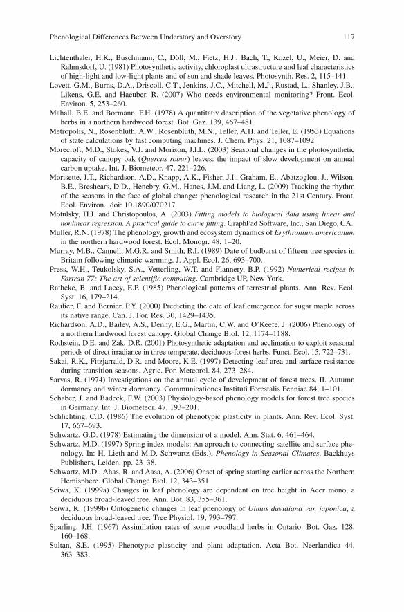
Phenological Differences Between Understory and Overstory 117
Lichtenthaler , H.K. , Buschmann , C. , Döll , M. , Fietz , H.J. , Bach , T. , Kozel , U. , Meier , D. and Rahmsdorf , U. (1981) Photosynthetic activity, chloroplast ultrastructure and leaf characteristics of high-light and low-light plants and of sun and shade leaves . Photosynth. Res. 2 , 115 – 141 .
Lovett , G.M. , Burns , D.A. , Driscoll , C.T. , Jenkins , J.C. , Mitchell , M.J. , Rustad , L. , Shanley , J.B. , Likens , G.E. and Haeuber , R. (2007) Who needs environmental monitoring? Front . Ecol. Environ. 5 , 253 – 260 .
Mahall , B.E. and Bormann , F.H. (1978) A quantitativ description of the vegetative phenology of herbs in a northern hardwood forest . Bot. Gaz. 139 , 467 – 481 .
Metropolis , N. , Rosenbluth , A.W. , Rosenbluth , M.N. , Teller , A.H. and Teller , E. (1953) Equations of state calculations by fast computing machines . J. Chem. Phys. 21 , 1087 – 1092 .
Morecroft , M.D. , Stokes , V.J. and Morison , J.I.L. (2003) Seasonal changes in the photosynthetic capacity of canopy oak (Quercus robur) leaves: the impact of slow development on annual carbon uptake . Int. J. Biometeor. 47 , 221 – 226 .
Morisette , J.T. , Richardson , A.D. , Knapp , A.K. , Fisher , J.I. , Graham , E. , Abatzoglou , J. , Wilson , B.E. , Breshears , D.D. , Henebry , G.M. , Hanes , J.M. and Liang , L. (2009) Tracking the rhythm of the seasons in the face of global change: phenological research in the 21st Century . Front. Ecol. Environ. , doi: 10.1890/070217 .
Motulsky , H.J. and Christopoulos , A. (2003) Fitting models to biological data using linear and nonlinear regression. A practical guide to curve fitting. GraphPad Software , Inc., San Diego , CA .
Muller , R.N. (1978) The phenology, growth and ecosystem dynamics of Erythronium americanum in the northern hardwood forest . Ecol. Monogr. 48 , 1 – 20 .
Murray , M.B. , Cannell , M.G.R. and Smith , R.I. (1989) Date of budburst of fifteen tree species in Britain following climatic warming . J. Appl. Ecol. 26 , 693 – 700 .
Press , W.H. , Teukolsky , S.A. , Vetterling , W.T. and Flannery , B.P. (1992) Numerical recipes in Fortran 77: The art of scientific computing . Cambridge UP , New York .
Rathcke , B. and Lacey , E.P. (1985) Phenological patterns of terrestrial plants . Ann. Rev. Ecol. Syst. 16 , 179 – 214 .
Raulier , F. and Bernier , P.Y. (2000) Predicting the date of leaf emergence for sugar maple across its native range . Can. J. For. Res. 30 , 1429 – 1435 .
Richardson , A.D. , Bailey , A.S. , Denny , E.G. , Martin , C.W. and O’Keefe , J. (2006) Phenology of a northern hardwood forest canopy . Global Change Biol. 12 , 1174 – 1188 .
Rothstein , D.E. and Zak , D.R. (2001) Photosynthetic adaptation and acclimation to exploit seasonal periods of direct irradiance in three temperate, deciduous-forest herbs . Funct. Ecol. 15 , 722 – 731 .
Sakai , R.K. , Fitzjarrald , D.R. and Moore , K.E. (1997) Detecting leaf area and surface resistance during transition seasons . Agric. For. Meteorol. 84 , 273 – 284 .
Sarvas , R. (1974) Investigations on the annual cycle of development of forest trees. II. Autumn dormancy and winter dormancy . Communicationes Instituti Forestalis Fenniae 84 , 1 – 101 .
Schaber , J. and Badeck , F.W. (2003) Physiology-based phenology models for forest tree species in Germany . Int. J. Biometeor. 47 , 193 – 201 .
Schlichting , C.D. (1986) The evolution of phenotypic plasticity in plants . Ann. Rev. Ecol. Syst. 17 , 667 – 693 .
Schwartz , G.D. (1978) Estimating the dimension of a model . Ann. Stat. 6 , 461 – 464 . Schwartz , M.D. (1997) Spring index models: An aproach to connecting satellite and surface phe-
nology . In: H. Lieth and M.D. Schwartz (Eds.), Phenology in Seasonal Climates . Backhuys Publishers , Leiden , pp. 23 – 38 .
Schwartz , M.D. , Ahas , R. and Aasa , A. (2006) Onset of spring starting earlier across the Northern Hemisphere . Global Change Biol. 12 , 343 – 351 .
Seiwa , K. (1999a) Changes in leaf phenology are dependent on tree height in Acer mono, a deciduous broad-leaved tree . Ann. Bot. 83 , 355 – 361 .
Seiwa , K. (1999b) Ontogenetic changes in leaf phenology of Ulmus davidiana var. japonica, a deciduous broad-leaved tree . Tree Physiol. 19 , 793 – 797 .
Sparling , J.H. (1967) Assimilation rates of some woodland herbs in Ontario . Bot. Gaz. 128 , 160 – 168 .
Sultan , S.E. (1995) Phenotypic plasticity and plant adaptation . Acta Bot. Neerlandica 44 , 363 – 383 .