Phylogeny - Lectures

Algorithmische Bioinformatik WS 11/12: , by R. Krause/ K. Reinert, 17. Oktober 2011, 23:12 1

Phylogeny

• Phylogenetic Trees, Maximum Parsimony, Bootstrapping

• Trees from Distances, Clustering, Neighbor Joining

• Probabilistic methods, Rate matrices

• Models of Sequence Evolution, Maximum Likelihood Trees

• Genome evolution

Phylogeny (2)

Recommende sources

• Dan Graur, Weng-Hsiun Li, Fundamentals of Molecular Evolution, Sinauer Associates

• D.W. Mount. Bioinformatics: Sequences and Genome analysis, 2001.

• R. Durbin, S. Eddy, A. Krogh & G. Mitchison, Biological sequence analysis, Cambridge, 1998

• J. Felsenstein: Inferring phylogenies. Sinauer Associates, 2004

Phylogeny, the tree of life

Essential molecular mechanisms as replication and gene expression were found to be similar among the orga-nisms studied so far. This favors the idea that all present day living organisms have evolved from a commonancestor. The relationship is called phylogeny and is represented by a phylogenetic tree.

(Figure from Doolittle, Science 284, 1999)

Reconstructing molecular phylogenies

2 Algorithmische Bioinformatik, WS 11/12, FU Berlin, by Roland Krause/Hannes Luz, 17. Oktober 2011, 23:12

Zuckerkandl and Pauling put forward to reconstruct the course of evolution by means of molecular with hugenumbers of characters.

E. Zuckerkandl and L. Pauling (1962), Molecular disease, evolution and genetic heterogeneity, In Horizons inBiochemistry, ed. M. Marsha and B. Pullman, Academic Press, pp. 189–225.

Euglena_anabaena AGAATCTGGGTTTGATTCCGGAGAGGGAGCCTGAGAGACGGCTAKhawkinea_quartana AGAATCAGGGTTCGATTCCGGAGAGGGAGCCTGAGAAACGGCTAPhacus_splendens AGAATTCGGGTTCGATTCCGGAGAGGGAGCCTGAGAAACGGCTAPhacus_oscillans AGAATCAGGGTTCGATTCCGGAGAGGGAGCCTGAGAGACGGCTAAstasia_longa AGAATCAGGGTTCGATTTCGGAGAGGGAGCCTCAGAGACGGCTALepocinclis_ovum AGAATCAGGGTTCGATTCCGGAGAGGGAGCCTGAGAGACGGCTAPeranema_trichophorum AGAATTAGGGTTTGATTCTGGAGAGGGAGCCTGAGAAATGGCTA

(A window of an alignment of small subunit rRNA genes)

Molecular Phylogeny (2)

• Traditional methods used morphological characteristics

• Advantages of molecular sequences

– DNA and amino acid sequences are strictly heritable units

– Unambigious description of molecular characters and character states

– Homology assessment is (relatively) easy

– Easier amenability to mathematical modeling and quantitative analysis

– Distant evolutionary relationships may be revealed

– Huge amounts of data available

Molecular Phylogeny (3)

Reconstructed molecular phylogenies are used to

• gain insights into molecular evolution

• predict gene functions

• detect various regimes of selective pressures (pharmacology)

• study the evolution of viruses (epidemiology)

Gene Tree and Species Tree

Algorithmische Bioinformatik, WS 11/12, FU Berlin, by Roland Krause/Hannes Luz, 17. Oktober 2011, 23:12 3

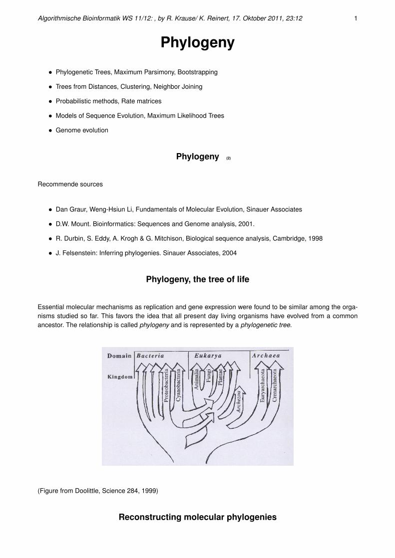
The traditional objective of a phylogenetic tree is to represent the evolutionary relationship between species.In molecular phylogeny, an alignment of homologous genes usually is input into the tree reconstruction. Thephylogeny of the species can be transferred from the gene tree, if the genes are orthologous.

Consider the evolution of alpha–hemoglobins in human, chimp and rat:

Gene Tree Species Tree

human chimp rathuman chimp ratα− α− α−

Gene Tree and Species Tree (2)

• Homologous genes have evolved from a common ancestor

• Orthologous genes have evolved from a common ancestor by a speciation event

• Paralogous genes have evolved from a common ancestor by a duplication event

α β

α− α− β−rat chimphuman

duplication

β–chimp is paralogous to α–rat (and to α–human) since the least common ancestor of the two genes corre-sponds to a duplication event.


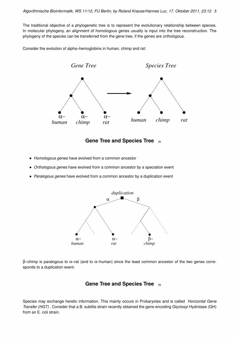
Species may exchange heretic information. This mainly occurs in Prokaryotes and is called Horizontal GeneTransfer (HGT) . Consider that a B. subtilis strain recently obtained the gene encoding Glyclosyl Hydrolase (GH)from an E. coli strain.


Species Tree

E. coli H. pylori B. subtilis

Gene Tree

E. coli B. subtilis H. pyloriGH− GH− GH−

HGT of GH

The gene tree and the species tree are incongruent and it is not possible to infer the species phylogeny basedon the gene tree for Glycosyl Hydrolase.


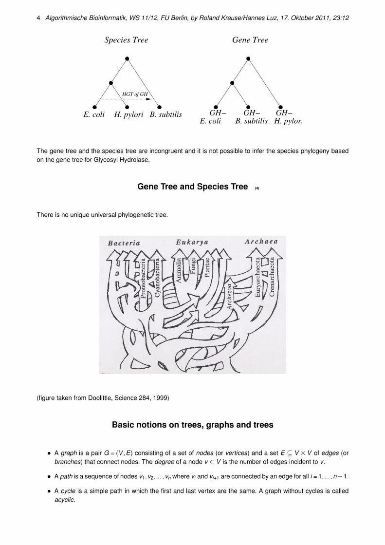
There is no unique universal phylogenetic tree.

(figure taken from Doolittle, Science 284, 1999)

Basic notions on trees, graphs and trees

• A graph is a pair G = (V ,E) consisting of a set of nodes (or vertices) and a set E ⊆ V ×V of edges (orbranches) that connect nodes. The degree of a node v ∈ V is the number of edges incident to v .

• A path is a sequence of nodes v1,v2, ... ,vn where vi and vi+1 are connected by an edge for all i = 1, ... ,n−1.

• A cycle is a simple path in which the first and last vertex are the same. A graph without cycles is calledacyclic.


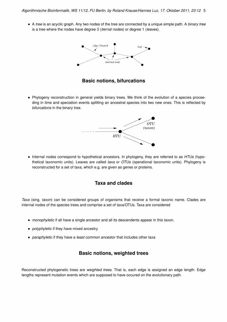
• A tree is an acyclic graph. Any two nodes of the tree are connected by a unique simple path. A binary treeis a tree where the nodes have degree 3 (iternal nodes) or degree 1 (leaves).

edge / branch leaf

internal node

Basic notions, bifurcations

• Phylogeny reconstruction in general yields binary trees. We think of the evolution of a species procee-ding in time and speciation events splitting an ancestral species into two new ones. This is reflected bybifurcations in the binary tree.

HTU

OTU(taxon)

• Internal nodes correspond to hypothetical ancestors. In phylogeny, they are referred to as HTUs (hypo-thetical taxonomic units). Leaves are called taxa or OTUs (operational taxonomic units). Phylogeny isreconstructed for a set of taxa, which e.g. are given as genes or proteins.

Taxa and clades

Taxa (sing. taxon) can be considered groups of organisms that receive a formal taxonic name. Clades areinternal nodes of the species trees and comprise a set of taxa/OTUs. Taxa are considered

• monophyletic if all have a single ancestor and all its descendents appear in this taxon.

• polyphyletic if they have mixed ancestry

• paraphyletic if they have a least common ancestor that includes other taxa

Basic notions, weighted trees

Reconstructed phylogenetic trees are weighted trees. That is, each edge is assigned an edge length. Edgelengths represent mutation events which are supposed to have occured on the evolutionary path.


A

3 3

B

C D

1

1 1

Differences in edge lenghts in the above tree reflect the fact, that the rates at which mutations accumulate in thesequences vary among the lineages to the taxa. This may be due to biological or environmental reasons.

Basic notions, binary tree vs. star tree

• Binary trees are said to be fully resolved. They donot exhibit multifurcations.

• A star tree only has one internal node with a mul-tifurcation (unresolved node, polytomy ). It is notresolved at all and provides no information aboutphylogenetic relationships.

• Reconstruction of phylogenies on data with aweak phylogenetic signal sometimes yields fullyresolved trees which look starlike.

Basic notions, rooting

Given a binary unrooted tree, one does not know wether an internal node is the ancestor or the descendant ofits neighboring internal node.

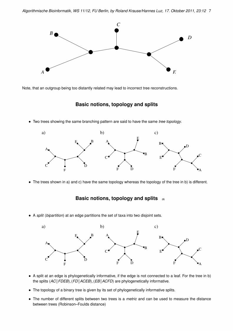
Sometimes it is possible to obtain external information that a certain taxon is more distantly related to the othertaxa than the other ones among themselves. Such a taxon is called outgroup. Adding a root node to the edge tothe outgroup then allows interpreting bifurcations with respect to time.


A

B

C

D

E

Note, that an outgroup being too distantly related may lead to incorrect tree reconstructions.

Basic notions, topology and splits

• Two trees showing the same branching pattern are said to have the same tree topology.

A

C

F

D

E B

A

C

F

DB

E

A

C

E

B

F D

a) b) c)

• The trees shown in a) and c) have the same topology whereas the topology of the tree in b) is different.

Basic notions, topology and splits (2)

• A split (bipartition) at an edge partitions the set of taxa into two disjoint sets.

A

C

F

D

E B

A

C

F

DB

E

A

C

E

B

F D

a) b) c)

• A split at an edge is phylogenetically informative, if the edge is not connected to a leaf. For the tree in b)the splits (AC‖FDEB), (FD‖ACEB), (EB‖ACFD) are phylogenetically informative.

• The topology of a binary tree is given by its set of phylogenetically informative splits.

• The number of different splits between two trees is a metric and can be used to measure the distancebetween trees (Robinson–Foulds distance)


Basic notions, Newick format

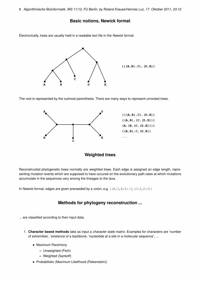
Electronically, trees are usually held in a readable text file in the Newick format.

A B

C

D E

(((A,B),C),(D,E))

The root is represented by the outmost parenthesis. There are many ways to represent unrooted trees.

A

B E

D

C

((A,B),C,(D,E))

(((A,B),C),(D,E))

((A,B),(C,(D,E)))

(A,(B,(C,(D,E))))

...

Weighted trees

Reconstructed phylogenetic trees normally are weighted trees. Each edge is assigned an edge length, repre-senting mutation events which are supposed to have occured on the evolutionary path.rates at which mutationsaccumulate in the sequences vary among the lineages to the taxa.

In Newick-format, edges are given preceeded by a colon, e.g. ((A:3,B:2):3,(C:2,D:3))

Methods for phylogeny reconstruction ...

... are classified according to their input data.

1. Character based methods take as input a character state matrix. Examples for characters are ’numberof extremities’, ’existence of a backbone, ’nucleotide at a site in a molecular sequence’, ...

• Maximum Parsimony

– Unweighted (Fitch)

– Weighted (Sankoff)

• Probabilistic (Maximum Likelihood (Felsenstein))


2. Distance based methods take as input a distance matrix, which is obtained by measuring the dissimilarityor the evolutionary distance between the taxa.

• Hierarchical clustering (UPGMA)

• Neighbor Joining

• Least Squares (Fitch–Margoliash)

Character state matrix

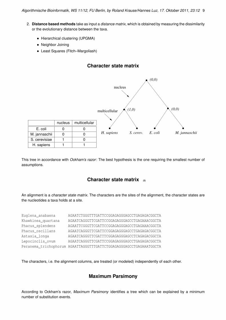
nucleus multicellular

E. coli 0 0M. jannaschii 0 0S. cerevisiae 1 0H. sapiens 1 1

H. sapiens S. cerev. E. coli M. jannaschii

nucleus

multicellular

(0,0)

(0,0)(1,0)

This tree in accordance with Ockham’s razor : The best hypothesis is the one requiring the smallest number ofassumptions.

Character state matrix (2)

An alignment is a character state matrix. The characters are the sites of the alignment, the character states arethe nucleotides a taxa holds at a site.

Euglena_anabaena AGAATCTGGGTTTGATTCCGGAGAGGGAGCCTGAGAGACGGCTAKhawkinea_quartana AGAATCAGGGTTCGATTCCGGAGAGGGAGCCTGAGAAACGGCTAPhacus_splendens AGAATTCGGGTTCGATTCCGGAGAGGGAGCCTGAGAAACGGCTAPhacus_oscillans AGAATCAGGGTTCGATTCCGGAGAGGGAGCCTGAGAGACGGCTAAstasia_longa AGAATCAGGGTTCGATTTCGGAGAGGGAGCCTCAGAGACGGCTALepocinclis_ovum AGAATCAGGGTTCGATTCCGGAGAGGGAGCCTGAGAGACGGCTAPeranema_trichophorum AGAATTAGGGTTTGATTCTGGAGAGGGAGCCTGAGAAATGGCTA

The characters, i.e. the alignment columns, are treated (or modeled) independently of each other.

Maximum Parsimony

According to Ockham’s razor, Maximum Parsimony identifies a tree which can be explained by a minimumnumber of substitution events.


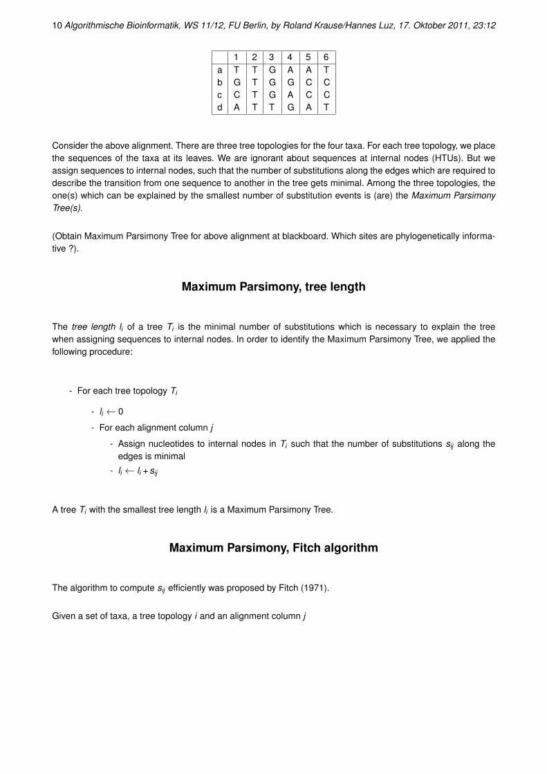
1 2 3 4 5 6a T T G A A Tb G T G G C Cc C T G A C Cd A T T G A T

Consider the above alignment. There are three tree topologies for the four taxa. For each tree topology, we placethe sequences of the taxa at its leaves. We are ignorant about sequences at internal nodes (HTUs). But weassign sequences to internal nodes, such that the number of substitutions along the edges which are required todescribe the transition from one sequence to another in the tree gets minimal. Among the three topologies, theone(s) which can be explained by the smallest number of substitution events is (are) the Maximum ParsimonyTree(s).

(Obtain Maximum Parsimony Tree for above alignment at blackboard. Which sites are phylogenetically informa-tive ?).

Maximum Parsimony, tree length

The tree length li of a tree Ti is the minimal number of substitutions which is necessary to explain the treewhen assigning sequences to internal nodes. In order to identify the Maximum Parsimony Tree, we applied thefollowing procedure:

- For each tree topology Ti

- li ← 0

- For each alignment column j

- Assign nucleotides to internal nodes in Ti such that the number of substitutions sij along theedges is minimal

- li ← li + sij

A tree Ti with the smallest tree length li is a Maximum Parsimony Tree.

Maximum Parsimony, Fitch algorithm

The algorithm to compute sij efficiently was proposed by Fitch (1971).

Given a set of taxa, a tree topology i and an alignment column j


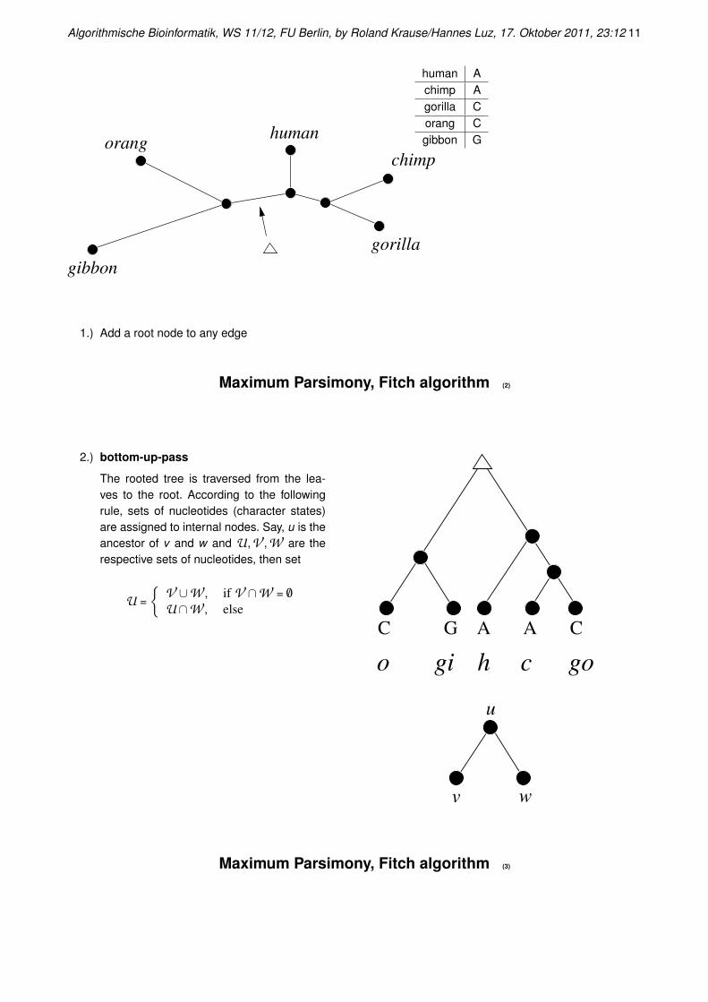
orang

gibbon

human

chimp

gorilla

human Achimp Agorilla Corang Cgibbon G

1.) Add a root node to any edge

Maximum Parsimony, Fitch algorithm (2)

2.) bottom-up-pass

The rooted tree is traversed from the lea-ves to the root. According to the followingrule, sets of nucleotides (character states)are assigned to internal nodes. Say, u is theancestor of v and w and U,V ,W are therespective sets of nucleotides, then set

U =

{V ∪W , if V ∩W = /0

U∩W , else

cgio h go

C G CA A

v

u

w



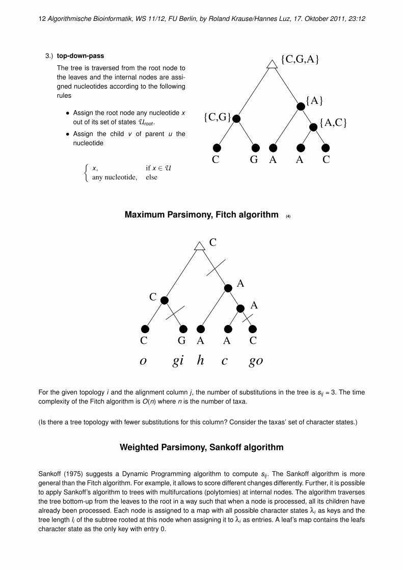
3.) top-down-pass

The tree is traversed from the root node tothe leaves and the internal nodes are assi-gned nucleotides according to the followingrules

• Assign the root node any nucleotide xout of its set of states Uroot .

• Assign the child v of parent u thenucleotide

{x , if x ∈Uany nucleotide, else

C CG A A

{A,C}{C,G}

{C,G,A}

{A}


cgio h go

CA AC G

C

C

A

A

For the given topology i and the alignment column j , the number of substitutions in the tree is sij = 3. The timecomplexity of the Fitch algorithm is O(n) where n is the number of taxa.

(Is there a tree topology with fewer substitutions for this column? Consider the taxas’ set of character states.)

Weighted Parsimony, Sankoff algorithm

Sankoff (1975) suggests a Dynamic Programming algorithm to compute sij . The Sankoff algorithm is moregeneral than the Fitch algorithm. For example, it allows to score different changes differently. Further, it is possibleto apply Sankoff’s algorithm to trees with multifurcations (polytomies) at internal nodes. The algorithm traversesthe tree bottom-up from the leaves to the root in a way such that when a node is processed, all its children havealready been processed. Each node is assigned to a map with all possible character states λi as keys and thetree length li of the subtree rooted at this node when assigning it to λi as entries. A leaf’s map contains the leafscharacter state as the only key with entry 0.


Weighted Parsimony, Sankoff algorithm (2)

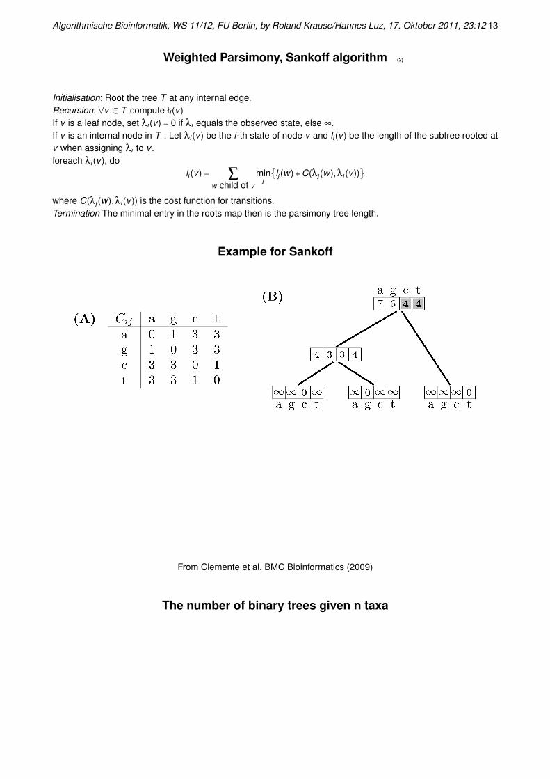
Initialisation: Root the tree T at any internal edge.Recursion: ∀v ∈ T compute łi (v )If v is a leaf node, set λi (v ) = 0 if λi equals the observed state, else ∞.If v is an internal node in T . Let λi (v ) be the i-th state of node v and li (v ) be the length of the subtree rooted atv when assigning λi to v .foreach λi (v ), do

li (v ) = ∑w child of v

minj{lj (w) + C(λj (w),λi (v ))}

where C(λj (w),λi (v )) is the cost function for transitions.Termination The minimal entry in the roots map then is the parsimony tree length.

Example for Sankoff

From Clemente et al. BMC Bioinformatics (2009)

The number of binary trees given n taxa


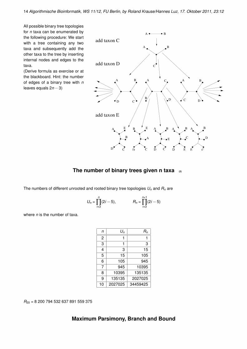
All possible binary tree topologiesfor n taxa can be enumerated bythe following procedure: We startwith a tree containing any twotaxa and subsequently add theother taxa to the tree by insertinginternal nodes and edges to thetaxa.(Derive formula as exercise or atthe blackboard. Hint: the numberof edges of a binary tree with nleaves equals 2n−3)

A

A B

B

C

BA A A

C

C

BC

DD

D

B

A E

B

CD

B E

A

CD

A B

E

CD

A B

C

D E

A B

D

E C

add taxon C

add taxon D

add taxon E

The number of binary trees given n taxa (2)

The numbers of different unrooted and rooted binary tree topologies Un and Rn are

Un =n

∏i=3

(2i−5), Rn =n+1

∏i=3

(2i−5)

where n is the number of taxa.

n Un Rn

2 1 13 1 34 3 155 15 1056 105 9457 945 103958 10395 1351359 135135 2027025

10 2027025 34459425

R20 = 8 200 794 532 637 891 559 375

Maximum Parsimony, Branch and Bound


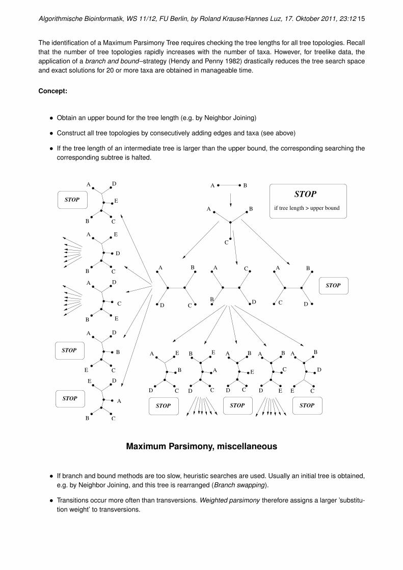
The identification of a Maximum Parsimony Tree requires checking the tree lengths for all tree topologies. Recallthat the number of tree topologies rapidly increases with the number of taxa. However, for treelike data, theapplication of a branch and bound–strategy (Hendy and Penny 1982) drastically reduces the tree search spaceand exact solutions for 20 or more taxa are obtained in manageable time.

Concept:

• Obtain an upper bound for the tree length (e.g. by Neighbor Joining)

• Construct all tree topologies by consecutively adding edges and taxa (see above)

• If the tree length of an intermediate tree is larger than the upper bound, the corresponding searching thecorresponding subtree is halted.

STOP

if tree length > upper bound

A E

B

D C

A

C

D

B

E

STOP

STOPSTOPSTOP

STOP

STOP

STOP

A

A B

B

C

BA A A

C

C

BC

DD D

B

B E

A

CD

A B

E

CD

A B

C

D E

A B

D

E C

A

CB

A D

B

A

C

D

C

D

B

E

D

E

C

B

E

E

A

Maximum Parsimony, miscellaneous

• If branch and bound methods are too slow, heuristic searches are used. Usually an initial tree is obtained,e.g. by Neighbor Joining, and this tree is rearranged (Branch swapping).

• Transitions occur more often than transversions. Weighted parsimony therefore assigns a larger ’substitu-tion weight’ to transversions.


• Maximum Parsimony is widely used. However, Maximum Parsim-ony does not take into account that the observed character statesof taxa being neighbors in the tree may have been multiply muta-ted. Maximum Parsimony therefore should only be applied to close-ly related sequences where the chance that multiple substitutionsoccured is small.

A

A

C

T

C

T

Inconsistency of Maximum Parsimony

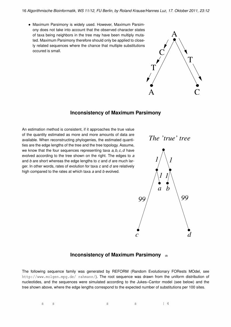
An estimation method is consistent, if it approaches the true valueof the quantity estimated as more and more amounts of data areavailable. When reconstructing phylogenies, the estimated quanti-ties are the edge lengths of the tree and the tree topology. Assume,we know that the four sequences representing taxa a,b,c,d haveevolved according to the tree shown on the right. The edges to aand b are short whereas the edge lengths to c and d are much lar-ger. In other words, rates of evolution for taxa c and d are relativelyhigh compared to the rates at which taxa a and b evolved.

The ’true’ tree

c

ba

d

1 1

1 1

99 99

Inconsistency of Maximum Parsimony (2)

The following sequence family was generated by REFORM (Random Evolutionary FORests MOdel, seehttp://www.molgen.mpg.de/ rahmann/). The root sequence was drawn from the uniform distribution ofnucleotides, and the sequences were simulated according to the Jukes–Cantor model (see below) and thetree shown above, where the edge lengths correspond to the expected number of substitutions per 100 sites.

s s s s | 4


a ATAAAGAGAAATGAGGACTACCCCAGACAAAATACTTAGTCATTAGAGGATGCACGAGAG |60b ATAAAGCGAAAGGAGGAGTACCCCAGACAAAATACTCAGTCATTAGAGGCTGCACGAGAG |60c AGCAAGAACTCGTCACCCTGCCACACACACAAAGCTGTATCGACCAACAAATGTCAAGAA |60d ATAATGTGATTGGGGCTGCGGGGCACTGGACATTCTTCGCCCGCAACTCCAGCACGAGCA |60

* * * * * * * *** * ** * * * * * ** * |21i i i i i i ii i | 9

s - sites where nucleotides in sequences a and b differ* - sites with identical nucleotides in c and di - phylogenetically informative sites

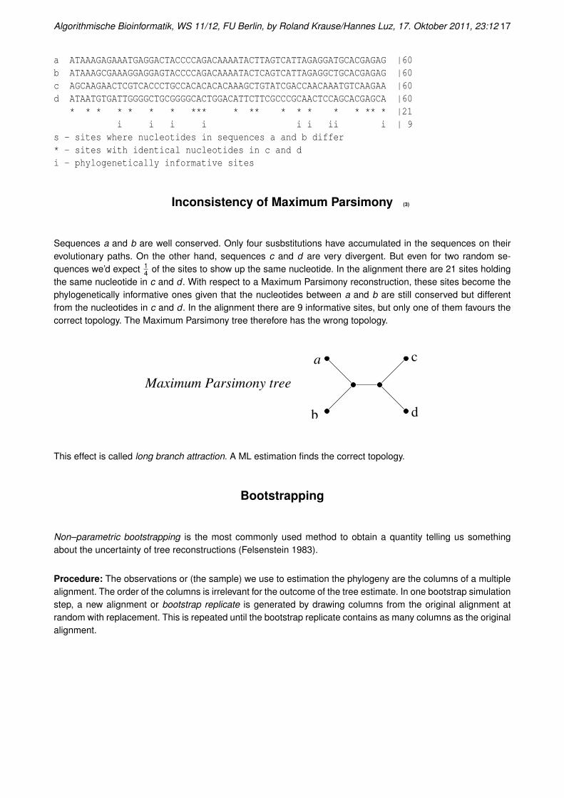
Inconsistency of Maximum Parsimony (3)

Sequences a and b are well conserved. Only four susbstitutions have accumulated in the sequences on theirevolutionary paths. On the other hand, sequences c and d are very divergent. But even for two random se-quences we’d expect 1

4 of the sites to show up the same nucleotide. In the alignment there are 21 sites holdingthe same nucleotide in c and d . With respect to a Maximum Parsimony reconstruction, these sites become thephylogenetically informative ones given that the nucleotides between a and b are still conserved but differentfrom the nucleotides in c and d . In the alignment there are 9 informative sites, but only one of them favours thecorrect topology. The Maximum Parsimony tree therefore has the wrong topology.

Maximum Parsimony tree

a

b

c

d

This effect is called long branch attraction. A ML estimation finds the correct topology.

Bootstrapping

Non–parametric bootstrapping is the most commonly used method to obtain a quantity telling us somethingabout the uncertainty of tree reconstructions (Felsenstein 1983).

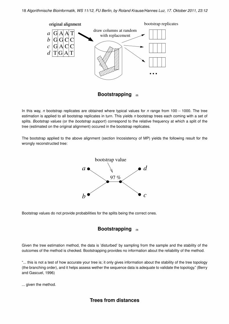
Procedure: The observations or (the sample) we use to estimation the phylogeny are the columns of a multiplealignment. The order of the columns is irrelevant for the outcome of the tree estimate. In one bootstrap simulationstep, a new alignment or bootstrap replicate is generated by drawing columns from the original alignment atrandom with replacement. This is repeated until the bootstrap replicate contains as many columns as the originalalignment.


a

b

c

d

��

��

��

��

��

��

��

��

original alignmentoriginal alignment bootstrap replicates

with replacement

...

draw columns at random

G G C CG A C CT G A T

G A A T

Bootstrapping (2)

In this way, n bootstrap replicates are obtained where typical values for n range from 100− 1000. The treeestimation is applied to all bootstrap replicates in turn. This yields n bootstrap trees each coming with a set ofsplits. Bootstrap values (or the bootstrap support) correspond to the relative frequency at which a split of thetree (estimated on the original alignment) occured in the bootstrap replicates.

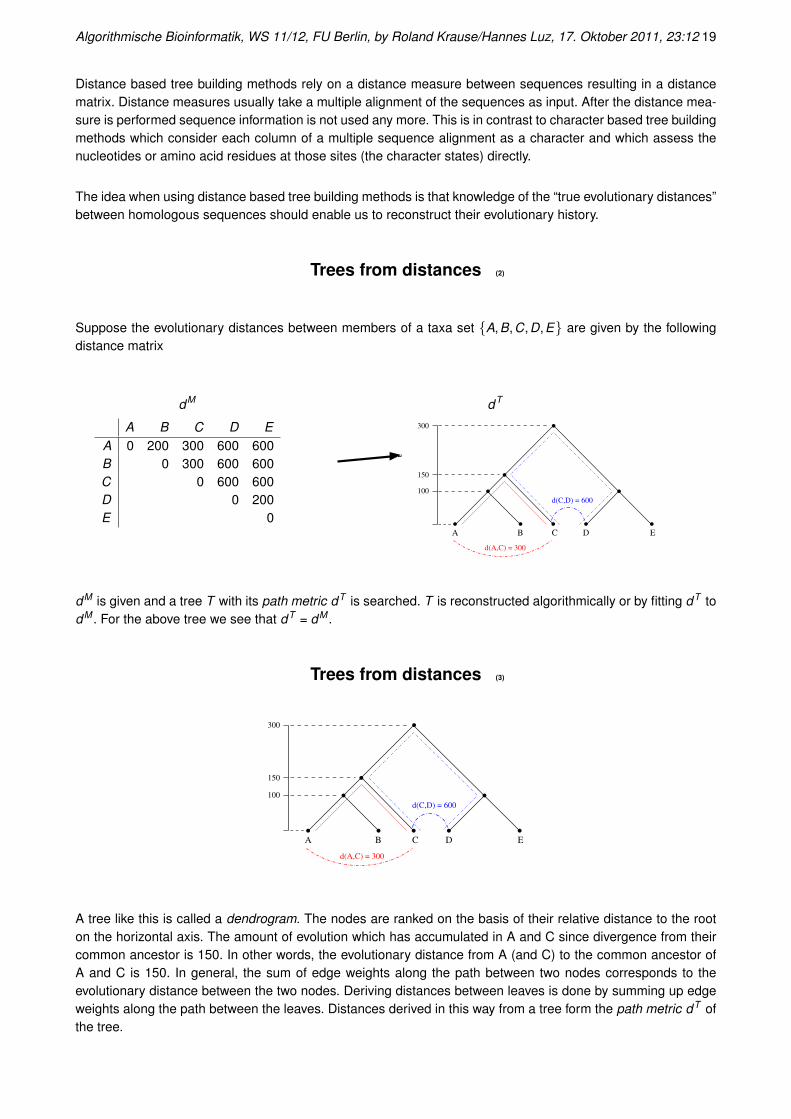
The bootstrap applied to the above alignment (section Incosistency of MP) yields the following result for thewrongly reconstructed tree:

a

bootstrap value

97 %

b

d

c

Bootstrap values do not provide probabilities for the splits being the correct ones.

Bootstrapping (3)

Given the tree estimation method, the data is ’disturbed’ by sampling from the sample and the stability of theoutcomes of the method is checked. Bootstrapping provides no information about the reliability of the method.

“... this is not a test of how accurate your tree is; it only gives information about the stability of the tree topology(the branching order), and it helps assess wether the sequence data is adequate to validate the topology.” (Berryand Gascuel, 1996)

... given the method.

Trees from distances


Distance based tree building methods rely on a distance measure between sequences resulting in a distancematrix. Distance measures usually take a multiple alignment of the sequences as input. After the distance mea-sure is performed sequence information is not used any more. This is in contrast to character based tree buildingmethods which consider each column of a multiple sequence alignment as a character and which assess thenucleotides or amino acid residues at those sites (the character states) directly.

The idea when using distance based tree building methods is that knowledge of the “true evolutionary distances”between homologous sequences should enable us to reconstruct their evolutionary history.

Trees from distances (2)

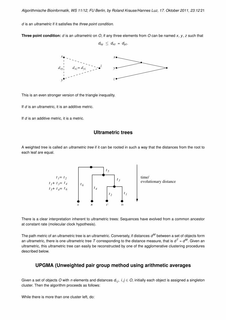
Suppose the evolutionary distances between members of a taxa set {A,B,C,D,E} are given by the followingdistance matrix

dM

A B C D EA 0 200 300 600 600B 0 300 600 600C 0 600 600D 0 200E 0

dT

100

150

300

A B C D E

d(C,D) = 600

d(A,C) = 300

dM is given and a tree T with its path metric dT is searched. T is reconstructed algorithmically or by fitting dT todM . For the above tree we see that dT = dM .

Trees from distances (3)

100

150

300

A B C D E

d(C,D) = 600

d(A,C) = 300

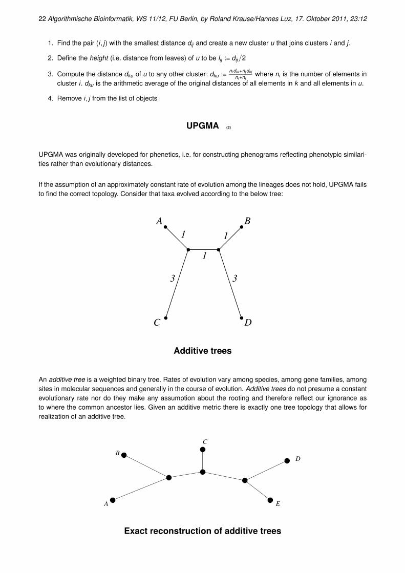
A tree like this is called a dendrogram. The nodes are ranked on the basis of their relative distance to the rooton the horizontal axis. The amount of evolution which has accumulated in A and C since divergence from theircommon ancestor is 150. In other words, the evolutionary distance from A (and C) to the common ancestor ofA and C is 150. In general, the sum of edge weights along the path between two nodes corresponds to theevolutionary distance between the two nodes. Deriving distances between leaves is done by summing up edgeweights along the path between the leaves. Distances derived in this way from a tree form the path metric dT ofthe tree.


Basic definitions, metric

Definition: A metric on a set of objects O is given by an assignment of a real number dij (a distance) to eachpair i , j ∈ O, where dij fulfills the following requirements:

(i) dij > 0 for i 6= j

(ii) dij = 0 for i = j

(iii) dij = dji ∀ i , j ∈ O

(iv) dij ≤ dik + dkj ∀ i , j ,k ∈ O

The latter requirement is called the triangle inequality

d ij

d ik d jk

i j

k

Basic definitions, additive metric (2)

Let d be a metric on O. d is an additive metric if it satisfies the four point condition (Bunemann 1971).

Four point condition: d is an additive metric on O, if any four elements from O can be named x , y , u and vsuch that

dxy + duv ≤ dxu + dyv = dxv + dyu.

dxy

x

y

u

v

d

xu

dyv d

d

uv

d xv

yu

+ < =+ +

The four point condition is a strengthened version of the triangle inequality. It implies that the path metric of atree is an additive metric.

Basic definitions, ultrametric (3)


d is an ultrametric if it satisfies the three point condition.

Three point condition: d is an ultrametric on O, if any three elements from O can be named x , y , z such that

dxy ≤ dxz = dyz .

dxy d d=xz yz

x

y

z

x

y

z

This is an even stronger version of the triangle inequality.

If d is an ultrametric, it is an additive metric.

If d is an additive metric, it is a metric.

Ultrametric trees

A weighted tree is called an ultrametric tree if it can be rooted in such a way that the distances from the root toeach leaf are equal.

evolutionary distancetime/

1t

4t

1tt =

2

4t

1t + t =

3

t + t = t5 4 6

A B C D

2

3

t

t

t

5t

6

There is a clear interpretation inherent to ultrametric trees: Sequences have evolved from a common ancestorat constant rate (molecular clock hypothesis).

The path metric of an ultrametric tree is an ultrametric. Conversely, if distances dM between a set of objects forman ultrametric, there is one ultrametric tree T corresponding to the distance measure, that is dT = dM . Given anultrametric, this ultrametric tree can easily be reconstructed by one of the agglomerative clustering proceduresdescribed below.

UPGMA (Unweighted pair group method using arithmetic averages

Given a set of objects O with n elements and distances di ,j , i , j ∈ O, initially each object is assigned a singletoncluster. Then the algorithm proceeds as follows:

While there is more than one cluster left, do:


1. Find the pair (i , j) with the smallest distance dij and create a new cluster u that joins clusters i and j .

2. Define the height (i.e. distance from leaves) of u to be lij := dij/2

3. Compute the distance dku of u to any other cluster: dku := ni dki +nj dkjni +nj

where ni is the number of elements incluster i . dku is the arithmetic average of the original distances of all elements in k and all elements in u.

4. Remove i , j from the list of objects

UPGMA (2)

UPGMA was originally developed for phenetics, i.e. for constructing phenograms reflecting phenotypic similari-ties rather than evolutionary distances.

If the assumption of an approximately constant rate of evolution among the lineages does not hold, UPGMA failsto find the correct topology. Consider that taxa evolved according to the below tree:

A

3 3

B

C D

1

1 1

Additive trees

An additive tree is a weighted binary tree. Rates of evolution vary among species, among gene families, amongsites in molecular sequences and generally in the course of evolution. Additive trees do not presume a constantevolutionary rate nor do they make any assumption about the rooting and therefore reflect our ignorance asto where the common ancestor lies. Given an additive metric there is exactly one tree topology that allows forrealization of an additive tree.

A

B

C

D

E

Exact reconstruction of additive trees


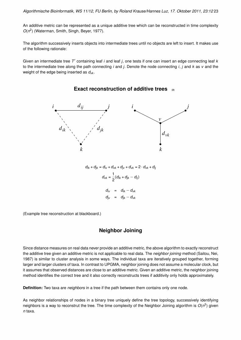
An additive metric can be represented as a unique additive tree which can be reconstructed in time complexityO(n2) (Waterman, Smith, Singh, Beyer, 1977).

The algorithm successively inserts objects into intermediate trees until no objects are left to insert. It makes useof the following rationale:

Given an intermediate tree T ′ containing leaf i and leaf j , one tests if one can insert an edge connecting leaf kto the intermediate tree along the path connecting i and j . Denote the node connecting i , j and k as v and theweight of the edge being inserted as dvk .

Exact reconstruction of additive trees (2)

d iji j

k

d ik d jk

i j

k

dvk

v

dik + djk = div + dvk + djv + dvk = 2 ·dvk + dij

dvk =12

(dik + djk −dij )

div = dik −dvk

djv = djk −dvk

(Example tree reconstruction at blackboard.)

Neighbor Joining

Since distance measures on real data never provide an additive metric, the above algorithm to exactly reconstructthe additive tree given an additive metric is not applicable to real data. The neighbor joining method (Saitou, Nei,1987) is similar to cluster analysis in some ways. The individual taxa are iteratively grouped together, forminglarger and larger clusters of taxa. In contrast to UPGMA, neighbor joining does not assume a molecular clock, butit assumes that observed distances are close to an additive metric. Given an additive metric, the neighbor joiningmethod identifies the correct tree and it also correctly reconstructs trees if additivity only holds approximately.

Definition: Two taxa are neighbors in a tree if the path between them contains only one node.

As neighbor relationships of nodes in a binary tree uniquely define the tree topology, successively identifyingneighbors is a way to reconstrut the tree. The time complexity of the Neighbor Joining algorithm is O(n3) givenn taxa.


Neighbor Joining (2)

The concept to identify neighbors is the following: A star tree is decomposed

B

C

A

D

E

a)

B

C

d

c

e

D

E

b)

A

a

bf

b)

B

A

E

C

D

c)

(A,B) (AB, D)

such that the tree length is minimized in each step. Consider the above star tree with N leaves shown in a). Thestar tree corresponds to the assumption that there is no clustering of taxa. In general there is a clustering of taxaand if so, the overall tree length (the sum of all branch lengths) SF of the true tree or the final NJ tree (see c)) issmaller than the overall tree length of the star tree S0.


The tree length of the tree with resolved neighbors A and B is

Sij =N

∑k=1k 6=i ,j

dki + dkj

2(N−2)+

dij

2+

N

∑k<l

k ,l 6=i ,j

dkl

N−2

where N is the number of taxa.Computation of SAB yields

SAB = (3a + 3b + 6f + 2c + 2d + 2e) · 16

+a + b

2+ (2c + 2d + 2e) · 1

3= a + b + f + c + d + e

S0

B

C

A

D

E

B

C

d

c

e

D

E A

a

bf

SAB


Theorem: Given an additive tree T . O is the set of leaves of T . Values of Sij are computed by means of the pathmetric dT . Then m,n ∈ O are neighbors in T , if Smn ≤ Sij ∀ i , j ∈ O.

Thus, computation of Sij for all pairs of taxa allows identifying neighbors given additive distances.


The neighbors are combined into one composite taxon and the procedure is repeated.

We rewrite Sij :

Sij =1

2(N−2)

(2 ·

N

∑k<l

k ,l 6=i ,j

dkl +N

∑k=1k 6=i ,j

(dki + dkj ))

+dij

2

=1

2(N−2)

(2 ·

N

∑i<j

dij − ri − rj

)+

dij

2

with ri := ∑Nk=1 dik .


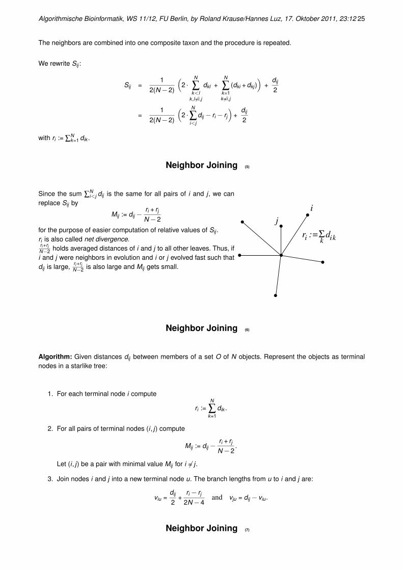
Since the sum ∑Ni<j dij is the same for all pairs of i and j , we can

replace Sij by

Mij := dij −ri + rj

N−2

for the purpose of easier computation of relative values of Sij .ri is also called net divergence.ri +rjN−2 holds averaged distances of i and j to all other leaves. Thus, ifi and j were neighbors in evolution and i or j evolved fast such thatdij is large, ri +rj

N−2 is also large and Mij gets small.

i

ri := kiΣdk

j


Algorithm: Given distances dij between members of a set O of N objects. Represent the objects as terminalnodes in a starlike tree:

1. For each terminal node i compute

ri :=N

∑k=1

dik .

2. For all pairs of terminal nodes (i , j) compute

Mij := dij −ri + rj

N−2.

Let (i , j) be a pair with minimal value Mij for i 6= j .

3. Join nodes i and j into a new terminal node u. The branch lengths from u to i and j are:

viu =dij

2+

ri − rj

2N−4and vju = dij − viu.



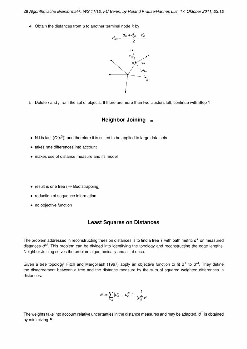
4. Obtain the distances from u to another terminal node k by

dku =dik + djk −dij

2.

j

u

k

i

i

uj

ukd

uv

v

5. Delete i and j from the set of objects. If there are more than two clusters left, continue with Step 1


• NJ is fast (O(n3)) and therefore it is suited to be applied to large data sets

• takes rate differences into account

• makes use of distance measure and its model

• result is one tree (→ Bootstrapping)

• reduction of sequence information

• no objective function

Least Squares on Distances

The problem addressed in reconstructing trees on distances is to find a tree T with path metric dT on measureddistances dM . This problem can be divided into identifying the topology and reconstructing the edge lengths.Neighbor Joining solves the problem algorithmically and all at once.

Given a tree topology, Fitch and Margoliash (1967) apply an objective function to fit dT to dM . They definethe disagreement between a tree and the distance measure by the sum of squared weighted differences indistances:

E := ∑i<j|dT

ij −dMij |2 ·

1(dM

ij )2

The weights take into account relative uncertanties in the distance measures and may be adapted. dT is obtainedby minimizing E .


How to obtain distances?

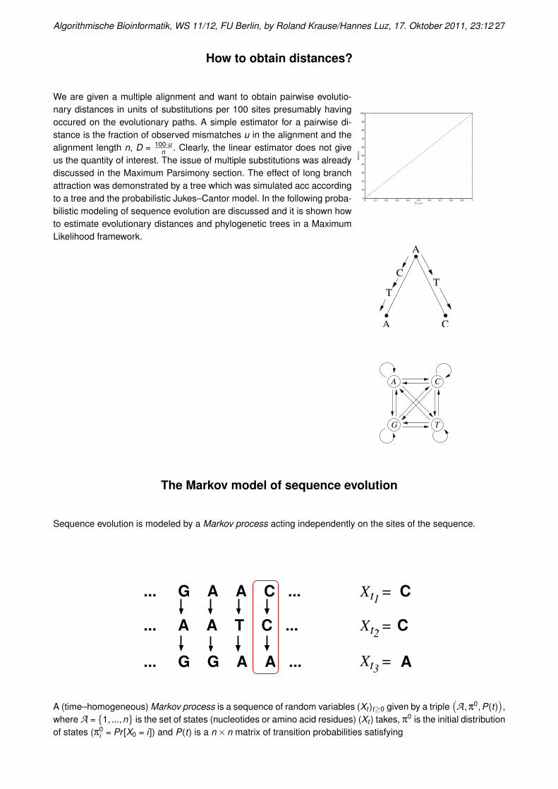
We are given a multiple alignment and want to obtain pairwise evolutio-nary distances in units of substitutions per 100 sites presumably havingoccured on the evolutionary paths. A simple estimator for a pairwise di-stance is the fraction of observed mismatches u in the alignment and thealignment length n, D = 100·u

n . Clearly, the linear estimator does not giveus the quantity of interest. The issue of multiple substitutions was alreadydiscussed in the Maximum Parsimony section. The effect of long branchattraction was demonstrated by a tree which was simulated acc accordingto a tree and the probabilistic Jukes–Cantor model. In the following proba-bilistic modeling of sequence evolution are discussed and it is shown howto estimate evolutionary distances and phylogenetic trees in a MaximumLikelihood framework.

0 0.1 0.2 0.3 0.4 0.5 0.6 0.7 0.8 0.9 10

10

20

30

40

50

60

70

80

90

100

D = u/n

dis

tan

ce

A

A

C

T

C

T

A C

G T

The Markov model of sequence evolution

Sequence evolution is modeled by a Markov process acting independently on the sites of the sequence.

t1

t2

t3

X =

X =

X =

... G G A A ... A

... G A A C ... C

... A A T C ... C

A (time–homogeneous) Markov process is a sequence of random variables (Xt )t≥0 given by a triple(A ,π0,P(t)

),

where A = {1, ...,n} is the set of states (nucleotides or amino acid residues) (Xt ) takes, π0 is the initial distributionof states (π0

i = Pr [X0 = i ]) and P(t) is a n×n matrix of transition probabilities satisfying


Pij (t) = Pr [Xt+s = j|Xs = i ] = Pr [Xt = j|X0 = i ]

The transition probability matrix

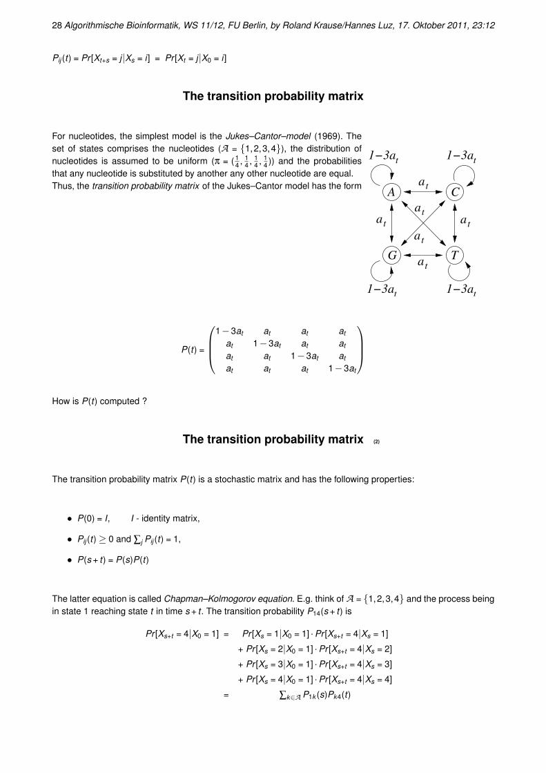
For nucleotides, the simplest model is the Jukes–Cantor–model (1969). Theset of states comprises the nucleotides (A = {1,2,3,4}), the distribution ofnucleotides is assumed to be uniform (π = ( 1

4 , 14 , 1

4 , 14 )) and the probabilities

that any nucleotide is substituted by another any other nucleotide are equal.Thus, the transition probability matrix of the Jukes–Cantor model has the form

at a

t

at

at

at

at

1−3at

1−3at

1−3at

1−3at

A C

G T

P(t) =

1−3at at at at

at 1−3at at at

at at 1−3at at

at at at 1−3at

How is P(t) computed ?

The transition probability matrix (2)

The transition probability matrix P(t) is a stochastic matrix and has the following properties:

• P(0) = I, I - identity matrix,

• Pij (t)≥ 0 and ∑j Pij (t) = 1,

• P(s + t) = P(s)P(t)

The latter equation is called Chapman–Kolmogorov equation. E.g. think of A = {1,2,3,4} and the process beingin state 1 reaching state t in time s + t . The transition probability P14(s + t) is

Pr [Xs+t = 4|X0 = 1] = Pr [Xs = 1|X0 = 1] ·Pr [Xs+t = 4|Xs = 1]

+ Pr [Xs = 2|X0 = 1] ·Pr [Xs+t = 4|Xs = 2]

+ Pr [Xs = 3|X0 = 1] ·Pr [Xs+t = 4|Xs = 3]

+ Pr [Xs = 4|X0 = 1] ·Pr [Xs+t = 4|Xs = 4]

= ∑k∈A P1k (s)Pk4(t)


The rate matrix

We assume that the probability transition matrix P(t) of a time continuous Markov chain is continuous anddifferentiable at any t > 0. I.e. the limit

Q := limt↘0

P(t)− It

exists. Q is known as the rate matrix or the generator of the Markov chain. For very small time periods h > 0,transition probabilities are approximated by

P(h) ≈ I + hQ

Pij (h) ≈ Qij ·h, i 6= j .

From the last equation we see, that the entries of Q may be interpreted as substitution rate.

The rate matrix (2)

From the Chapman-Kolmogorov equation we get

ddt

P(t) = limh↘0

P(t + h)−P(t)h

= limh↘0

P(t)P(h)−P(t)Ih

= P(t) limh↘0

P(h)−P(0)h

ddt

P(t) = P(t)Q = QP(t).

Under the initial condition P(0) = I the differential equation can be solved and yields (as in the one–dimensionalcase)

P(t) = exp(tQ) =∞

∑k=0

Qk tk

k !.

Transition probabilities for any t > 0 are computed from the matrix Q.

The rate matrix (3)

Recall, that for very small h we have P(h)≈ I + hQ.

Q has the following properties:

• Pij (h)≥ 0 ⇒ Qij ≥ 0 for i 6= j

• ∑j Pij (h) = 1 and Qij ≥ 0, i 6= j ⇒ Qii ≤ 0


• 1 = ∑j Pij (h) = 1 + ∑j Qij ⇒ ∑j Qij = 0, Qii =−∑j 6=i Qij

The rate matrix (4)

The rate matrix of the Jukes–Cantor model is

Q =

−3α α α α

α −3α α α

α α −3α α

α α α −3α

.

where α≥ 0.

Due to the simple structure of Q, exp(tQ) can be calculated explicitly. The transition probability matrix is

P(t) =

1−3at at at at

at 1−3at at at

at at 1−3at at

at at at 1−3at

,

where

at =1−exp(−4αt)

4

Stationarity and reversibility

A (probability) distribution of states π is called stationary, if the probability to observe a certain state remains thesame for all time points, i.e.

πj = ∑i∈A

πiPij (t) and π = πP(t) ∀ t .

For very small h and stationarity,

πj = ∑i πiPij (h) = πj + ∑i πiQij ⇒ ∑i πiQij = 0 and πQ = 0.

That is, if we are given Q, we are given all model parameters.

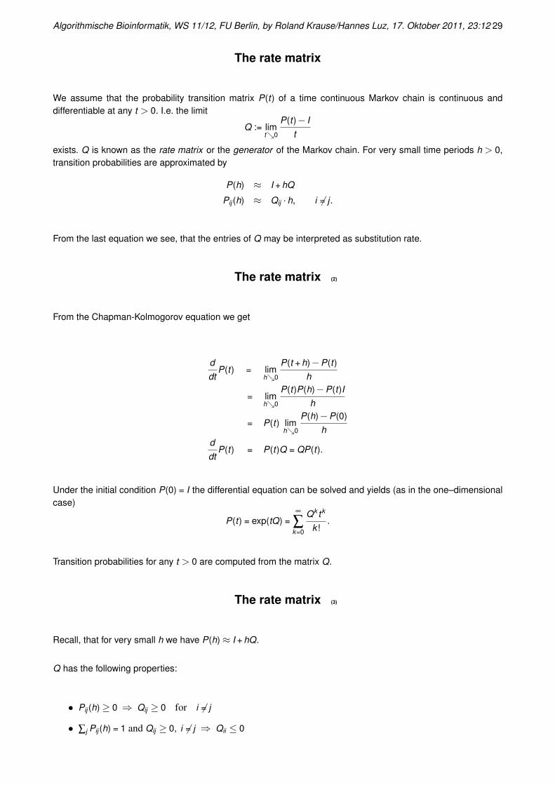
In general, π is not uniform. Modeling the evolution of state i reaching state j in time t by thesame process as state j reaching state i in time t is called reversibility :πiPij (t) = πjPji (t) (detailed balance)

A C

The stationary distribution of a Markov process which obeyes detailed balance is also called the equilibriumdistribution. When tree estimation under a reversible model is concerned, reversibility implies that we are ignorantabout the root position.


Calibrating the rate matrix

If we are given Q, we are given all model parameters. All of the above equations hold, if Q is multiplied with aconstant. Explicit model parameters fix the speed of the process. In other words: The model parameters holdsubstitution rates. And rates hold the information how many substitutions per time unit one expects.

The rate matrix is calibrated to PEM (percent of expected mutations)–units. 1 PEM is the time (or evolutionarydistance) where one substitution event per 100 sites is expected to have occured.

Given Q, one expects E = ∑i πi ∑j 6=i Qij =−∑i πiQii substitution events per time unit.

The Jukes–Cantor rate matrix Q is calibrated to PEM–units by setting E = 1100 ⇔−4 · 1

4 ·−3α = 1100 ⇔ α = 1

300 .

Evolutionary Markov Process (Xt )with stationary distribution π (π–EMP)

Müller, Rahmann and Vingron have summarized the properties of a Markov process being suited to describe thesubstitution process at a site of a molecular sequence. A π–EMP has the following properties:

• (Xt ) is time homogeneous.

Pij (t) = Prob[Xs+t = j|Xs = i ] = Prob[Xt = j|X0 = i ].

• (Xt ) is stationary w.r.t. π.πj = ∑i πiPij (t), π = πP(t) ∀ t .

• (Xt ) is reversible. πiPij (t) = πjPji (t).

• (Xt ) is calibrated to 1 PEM, the evolutionary distance where one substitution event per 100 sites is expec-ted to have occured.

The Jukes–Cantor correction

The linear estimator D = 100·un (u-mismatches, n- sequence length) for the distance between two DNA sequences

is ignorant about the putative occurence of multiple substitutions. The Jukes–Cantor correction provides a for-mula for the evolutionary distance d of two DNA sequences, i.e. d holds the number of substitutions which areexpected to have occured per 100 sites given the observed mismatches. (d is measured in time units of theMarkov process).

The probability p to observe that a nucleotide is not substituted after time t is

p = ∑i πiPii (t) = 4 · 14 (1−3at ) = 1− 3

4 (1−exp(−4αt)) = 1+3exp(−4αt)4

There are u mismatches among n sites. That is, we observe p = 1− un . Calibration to PEM–units and setting

t = d yields

1− un

=1 + 3exp(−4d/300)

4


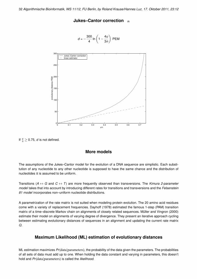
Jukes–Cantor correction (2)

d =−3004

ln

(1− 4u

3n

)PEM

0 0.1 0.2 0.3 0.4 0.5 0.6 0.70

50

100

150

200

250

300

u/n

evo

lutio

na

ry d

ista

nce

PE

M

Jukes−Cantor−correctionlinear estimator

If un ≥ 0.75, d is not defined.

More models

The assumptions of the Jukes–Cantor model for the evolution of a DNA sequence are simplistic. Each substi-tution of any nucleotide to any other nucleotide is supposed to have the same chance and the distribution ofnucleotides π is assumed to be uniform.

Transitions (A↔ G and C ↔ T ) are more frequently observed than transversions. The Kimura 2-parametermodel takes that into account by introducing different rates for transitions and transversions and the Felsenstein81 model incorporates non–uniform nucleotide distributions.

A parametrization of the rate matrix is not suited when modeling protein evolution. The 20 amino acid residuescome with a variety of replacement frequencies. Dayhoff (1978) estimated the famous 1-step (PAM) transitionmatrix of a time–discrete Markov chain on alignments of closely related sequences. Müller and Vingron (2000)estimate their model on alignments of varying degree of divergence. They present an iterative approach cyclingbetween estimating evolutionary distances of sequences in an alignment and updating the current rate matrixQ.

Maximum Likelihood (ML) estimation of evolutionary distances

ML estimation maximizes Pr (data|parameters), the probability of the data given the parameters. The probabilitiesof all sets of data must add up to one. When holding the data constant and varying in parameters, this doesn’thold and Pr (data|parameters) is called the likelihood.


Consider the following alignment:A G CA L A

The probability of observing the alignment D (the data) with distance t given the Markov model M is

Pr(D|t ,M ) = πAPAA(t) ·πGPGL(t) ·πRPCA(t).

Consider Pr(D|t ,M ) as likelihood function depending on distance t :

logL(t) = logPr(D|t ,M )

The evolutionary distance is estimated as distance t̂ maximizing the likelihood function.

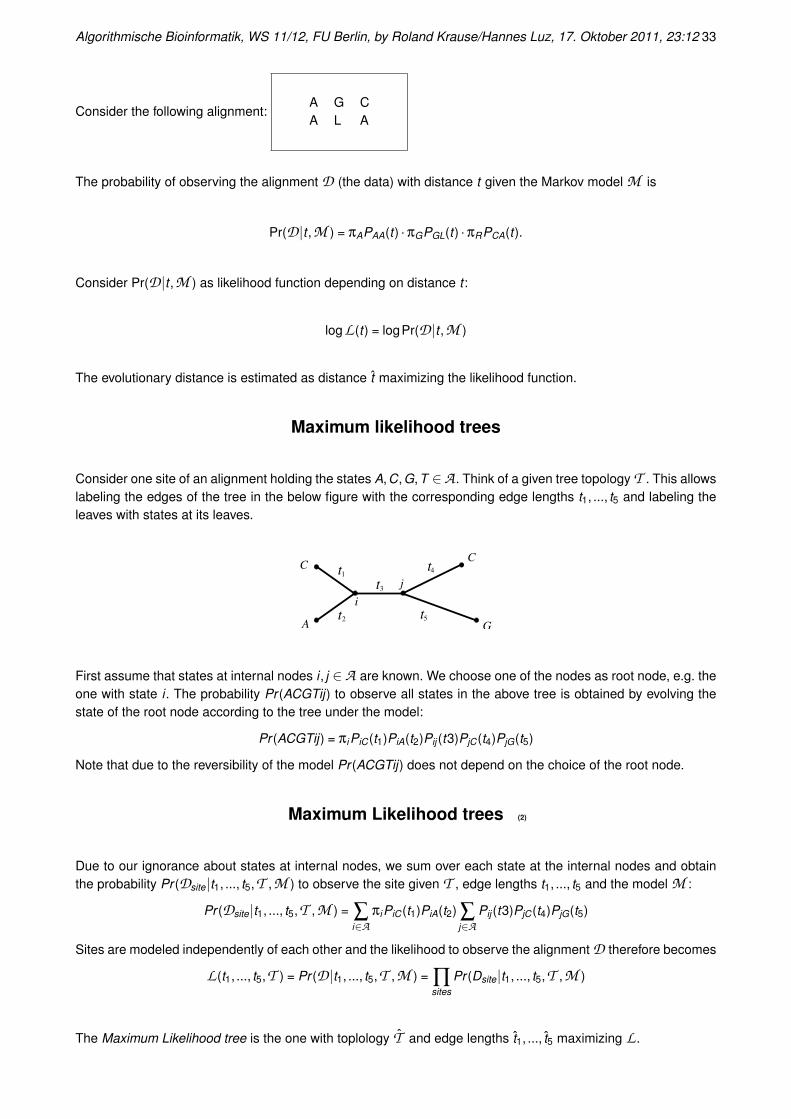
Maximum likelihood trees

Consider one site of an alignment holding the states A,C,G,T ∈A . Think of a given tree topology T . This allowslabeling the edges of the tree in the below figure with the corresponding edge lengths t1, ..., t5 and labeling theleaves with states at its leaves.

2t

3t

4t

5t

1t

A

CC

G

i

j

First assume that states at internal nodes i , j ∈A are known. We choose one of the nodes as root node, e.g. theone with state i . The probability Pr (ACGTij) to observe all states in the above tree is obtained by evolving thestate of the root node according to the tree under the model:

Pr (ACGTij) = πiPiC(t1)PiA(t2)Pij (t3)PjC(t4)PjG(t5)

Note that due to the reversibility of the model Pr (ACGTij) does not depend on the choice of the root node.

Maximum Likelihood trees (2)

Due to our ignorance about states at internal nodes, we sum over each state at the internal nodes and obtainthe probability Pr (Dsite|t1, ..., t5,T ,M ) to observe the site given T , edge lengths t1, ..., t5 and the model M :

Pr (Dsite|t1, ..., t5,T ,M ) = ∑i∈A

πiPiC(t1)PiA(t2) ∑j∈A

Pij (t3)PjC(t4)PjG(t5)

Sites are modeled independently of each other and the likelihood to observe the alignment D therefore becomes

L(t1, ..., t5,T ) = Pr (D|t1, ..., t5,T ,M ) = ∏sites

Pr (Dsite|t1, ..., t5,T ,M )

The Maximum Likelihood tree is the one with toplology T̂ and edge lengths t̂1, ..., t̂5 maximizing L .


Maximum Likelihood trees (3)

• Sometimes the model parameters are also varied when optimizing the likelihood, that is L =L(t1, ..., tn,T ,M ).

• For ease of computation log L instead of L is maximized.

• The likelihood of a site is efficiently computed by recursion (Felsenstein 1981). A rooted tree topology istraversed from the leaves to the root. Each internal node k is assigned a conditional likelihood Ls,k as thelikelihood of the subtree rooted at k , given that node k has state (nucleotide) s ∈ A .

Maximum likelihood trees (4)

• ML estimation is a powerful concept to infer phylogenies. ML tree estimation has proven to be robust evenwhen (evolutionary) model assumptions are violated.

• ML is computationally the most expensive tree reconstruction method.

• A very fast and widely used heuristic to reduce the tree search space is Quartet Puzzling (Strimmer, v.Haeseler 1996, see also http://www.tree-puzzle.de/). The optimal tree for all subsets of sequencesconsisting only of four sequences (=quartet) is computed. Subsequently, the quartet trees are combinedinto a larger tree for all sequences.

Documents

Phylogeny - Lectures