Embed Size (px)
Citation preview

PHYS 263
Exercises with solutions
Jakob J. Stamnes
—————————————————————–Department of Physics and Technology, University of Bergen, 5007 Bergen.
Tlf: 55 58 28 18. Fax: 55 58 94 40. E-post: [email protected]
Spring 2004
PHYS 263 side 1
Contents
I PHYS 263 4
1 Vector relations 5
2 Variable change in the wave equation 7
3 Laplacian operator for spherically symmetric functions 9
4 Waves and wave packets 114.1 Superposition of two harmonic plane waves . . . . . . . . . . . . . . . . . . . . . . . 114.2 Group velocity and phase velocity . . . . . . . . . . . . . . . . . . . . . . . . . . . . 124.3 Dispersion and energy propagation . . . . . . . . . . . . . . . . . . . . . . . . . . . . 13
5 Connection between group velocity, phase velocity, and refractive index 145.1 Group velocity as a function of phase velocity and refractive index . . . . . . . . . . 145.2 The group velocity is less than the speed of light in vacuum . . . . . . . . . . . . . . 14
6 Propagation in a dispersive medium 166.1 Propagation of a quasi-monochromatic wave . . . . . . . . . . . . . . . . . . . . . . . 166.2 The shape and speed of the wave . . . . . . . . . . . . . . . . . . . . . . . . . . . . . 176.3 Alternative way to proceed . . . . . . . . . . . . . . . . . . . . . . . . . . . . . . . . 17
7 Polarisation and rotation of co-ordinate system 197.1 Maximum and minimum values . . . . . . . . . . . . . . . . . . . . . . . . . . . . . . 197.2 Rotation of co-ordinate system . . . . . . . . . . . . . . . . . . . . . . . . . . . . . . 207.3 Simplification of the expression for the ellipse . . . . . . . . . . . . . . . . . . . . . . 22
8 Phase velocity and group velocity for surface waves on water 248.1 Separation of variables . . . . . . . . . . . . . . . . . . . . . . . . . . . . . . . . . . . 258.2 Dispersion relation . . . . . . . . . . . . . . . . . . . . . . . . . . . . . . . . . . . . . 268.3 Phase velocity and group velocity . . . . . . . . . . . . . . . . . . . . . . . . . . . . . 278.4 The phase velocity of surface waves in water of infinite depth . . . . . . . . . . . . . 278.5 The phase velocity of surface waves in water of finite depth . . . . . . . . . . . . . . 288.6 The refractive index . . . . . . . . . . . . . . . . . . . . . . . . . . . . . . . . . . . . 298.7 The wavelength in water of infinite depth . . . . . . . . . . . . . . . . . . . . . . . . 308.8 The wavelength in water of finite depth . . . . . . . . . . . . . . . . . . . . . . . . . 318.9 Refraction of waves that propagate towards a beach . . . . . . . . . . . . . . . . . . 31
9 Fresnel’s formulas 339.1 Rewriting of Fresnel’s formulas . . . . . . . . . . . . . . . . . . . . . . . . . . . . . . 339.2 The sign of the reflection and transmission coefficients . . . . . . . . . . . . . . . . . 35
10 Reflectivity and transmissivity 3610.1 Energy conservation for TE and TM components . . . . . . . . . . . . . . . . . . . . 3610.2 Energy conservation . . . . . . . . . . . . . . . . . . . . . . . . . . . . . . . . . . . . 37

PHYS 263 side 2
11 Total reflection 1 3911.1 Transmitted magnetic field . . . . . . . . . . . . . . . . . . . . . . . . . . . . . . . . 3911.2 Transmitted Poynting vector . . . . . . . . . . . . . . . . . . . . . . . . . . . . . . . 4111.3 Time average of the Poynting vector . . . . . . . . . . . . . . . . . . . . . . . . . . . 43
12 Fresnel’s rhomb 4412.1 Solution for sin θi. . . . . . . . . . . . . . . . . . . . . . . . . . . . . . . . . . . . . . 4412.2 Phase difference of 45◦, n = 1/1.52 = 0.6579 . . . . . . . . . . . . . . . . . . . . . . . 4512.3 Phase difference of 45◦, n = 1/1.49 = 0.6711 . . . . . . . . . . . . . . . . . . . . . . . 4512.4 Maximum phase difference . . . . . . . . . . . . . . . . . . . . . . . . . . . . . . . . . 4512.5 Phase differences of 45◦ and 90◦ . . . . . . . . . . . . . . . . . . . . . . . . . . . . . 46
13 Total reflection 2 48
II FYS 263 del II 50
14 Reflection and refraction of a plane acoustical wave 5114.1 Snell’s law and the reflection law . . . . . . . . . . . . . . . . . . . . . . . . . . . . . 5214.2 Reflection and transmission coefficients . . . . . . . . . . . . . . . . . . . . . . . . . . 5214.3 Comparison with electromagnetic waves . . . . . . . . . . . . . . . . . . . . . . . . . 53
15 Fourier representation of a real function 54
16 Convolution theorem, autocorrelation theorem, and Parseval’s theorem 5516.1 Convolution . . . . . . . . . . . . . . . . . . . . . . . . . . . . . . . . . . . . . . . . . 5516.2 Autocorrelation . . . . . . . . . . . . . . . . . . . . . . . . . . . . . . . . . . . . . . . 5616.3 Parseval’s theorem . . . . . . . . . . . . . . . . . . . . . . . . . . . . . . . . . . . . . 57
17 Angular-spectrum representation of a spherical wave (Weyl’s formula) 5817.1 The angular spectrum . . . . . . . . . . . . . . . . . . . . . . . . . . . . . . . . . . . 5917.2 Weyl’s plane-wave expansion of a spherical wave . . . . . . . . . . . . . . . . . . . . 59
18 The Airy diffraction pattern 61
19 Integrated energy of the Airy diffraction pattern 6219.1 Total differential for J2
1 (x)x . . . . . . . . . . . . . . . . . . . . . . . . . . . . . . . . . 62
19.2 Encircled energy . . . . . . . . . . . . . . . . . . . . . . . . . . . . . . . . . . . . . . 62
20 Fresnel diffraction through an infinitely large circular aperture 6420.1 Change of variable: vt→ x . . . . . . . . . . . . . . . . . . . . . . . . . . . . . . . . 6420.2 Infinitely large aperture . . . . . . . . . . . . . . . . . . . . . . . . . . . . . . . . . . 65
21 Diffraction by a half-plane 6721.1 Detour parameter associated with the incident wave . . . . . . . . . . . . . . . . . 6721.2 Detour parameter associated with the reflected wave . . . . . . . . . . . . . . . . . . 67
22 Diffraction through a circular aperture – axial intensity 70
23 Poisson’s spot 7223.1 Diffraction of a spherical wave through a circular aperture . . . . . . . . . . . . . . . 7323.2 Opaque disc . . . . . . . . . . . . . . . . . . . . . . . . . . . . . . . . . . . . . . . . . 7423.3 Proof of Babinet’s principle . . . . . . . . . . . . . . . . . . . . . . . . . . . . . . . . 7423.4 Axial field - incident plane wave . . . . . . . . . . . . . . . . . . . . . . . . . . . . . . 7423.5 Axial field - incident spherical wave . . . . . . . . . . . . . . . . . . . . . . . . . . . . 75

PHYS 263 side 3
24 Fraunhofer diffraction at oblique incidence and interference between the fieldsdiffracted through two apertures 7624.1 Fourier representation at oblique incidence . . . . . . . . . . . . . . . . . . . . . . . . 7624.2 Airy diffraction pattern at oblique incidence . . . . . . . . . . . . . . . . . . . . . . . 7724.3 Aperture displacement . . . . . . . . . . . . . . . . . . . . . . . . . . . . . . . . . . . 7924.4 Interference . . . . . . . . . . . . . . . . . . . . . . . . . . . . . . . . . . . . . . . . . 8024.5 Example . . . . . . . . . . . . . . . . . . . . . . . . . . . . . . . . . . . . . . . . . . . 80

PHYS 263 side 4
Part I
PHYS 263
PHYS 263 side 5
Chapter 1
Vector relations
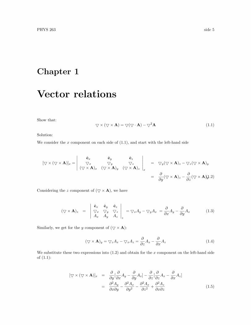
Show that:5× (5×A) = 5(5 ·A)−52A (1.1)
Solution:
We consider the x component on each side of (1.1), and start with the left-hand side
[5× (5×A)]x =
∣∣∣∣∣∣ex ey ez5x 5y 5z
(5×A)x (5×A)y (5×A)z
∣∣∣∣∣∣x
= 5y(5×A)z −5z(5×A)y
=∂
∂y(5×A)z −
∂
∂z(5×A)y(1.2)
Considering the z component of (5×A), we have
(5×A)z =
∣∣∣∣∣∣ex ey ez5x 5y 5z
Ax Ay Az
∣∣∣∣∣∣z
= 5xAy −5yAx =∂
∂xAy −
∂
∂yAx (1.3)
Similarly, we get for the y component of (5×A):
(5×A)y = 5zAx −5xAz =∂
∂zAx −
∂
∂xAz (1.4)
We substitute these two expressions into (1.2) and obtain for the x component on the left-hand sideof (1.1):
[5× (5×A)]x =∂
∂y[∂
∂xAy −
∂
∂yAx]−
∂
∂z[∂
∂zAx −
∂
∂xAz]
=∂2Ay∂x∂y
− ∂2Ax∂y2
− ∂2Ax∂z2
+∂2Az∂x∂z
(1.5)

PHYS 263 side 6
For the right-hand side of (1.1) we have:
[5(5 ·A)−52A]x = 5x(∂Ax∂x
+∂Ay∂y
+∂Az∂z
)− (∂2
∂x2+
∂2
∂y2+
∂2
∂z2)Ax
=∂2Ax∂x2
+∂2Ay∂x∂y
+∂2Az∂x∂z
− ∂2Ax∂x2
− ∂2Ax∂y2
− ∂2Ax∂z2
=∂2Ay∂x∂y
+∂2Az∂x∂z
− ∂2Ax∂y2
− ∂2Ax∂z2
= [5× (5×A)]x (1.6)
Thus, as far the x component of (1.1) is concerned, the right-hand side is equal to the left-hand side.The proof for the y or z component of (1.1) follows in a similar manner.
PHYS 263 side 7
Chapter 2
Variable change in the waveequation
In chapter 4.1 in the lecture notes [?] the equation
∂2V
∂p∂q= 0 (2.1)
constitutes an important part of the derivation of a general solution of the wave equation.
Show that
∂2V
∂ζ2− 1v2
∂2V
∂t2= 0 (2.2)
can be written in the form:
∂2V
∂p∂q= 0 (2.3)
where p = ζ − vt and q = ζ + vt.
Solution:
p = ζ − vt ; q = ζ + vt. (2.4)
∂p
∂ζ=∂q
∂ζ= 1
∂p
∂t= −v
∂q
∂t= v (2.5)
The first term in 2.2 becomes:
PHYS 263 side 8
∂V
∂ζ=
∂V
∂p
∂p
∂ζ+∂V
∂q
∂q
∂ζ=∂V
∂p+∂V
∂q
∂2V
∂ζ2=
∂
∂p
[∂V
∂p+∂V
∂q
]∂p
∂ζ+
∂
∂q
[∂V
∂p+∂V
∂q
]∂q
∂ζ=∂2V
∂p2+∂2V
∂q2+ 2
∂2V
∂p∂q(2.6)
The second term in 2.2 becomes:
∂V
∂t=
∂V
∂p
∂p
∂t+∂V
∂q
∂q
∂t= −v
[∂V
∂p− ∂V
∂q
]∂2V
∂t2= −v
{∂
∂p
[∂V
∂p− ∂V
∂q
]∂p
∂t+
∂
∂q
[∂V
∂p− ∂V
∂q
]∂q
∂t
}= −v
{∂
∂p
[∂V
∂p− ∂V
∂q
](−v) +
∂
∂q
[∂V
∂p− ∂V
∂q
]v
}⇒ − 1
v2
∂2V
∂t2= −∂
2V
∂p2− ∂2V
∂q2+ 2
∂2V
∂p∂q(2.7)
Adding 2.6 and 2.7, we get:
∂2V
∂ζ2− 1v2
∂2V
∂t2= 4
∂2V
∂p∂q= 0 (2.8)
which was to be proven.
PHYS 263 side 9
Chapter 3
Laplacian operator for sphericallysymmetric functions
Show that the Laplacian operator has the following form in spherical co-ordinates for a functionwith spherical symmetry (this form is used in section 4.2 in the lecture notes [?]):
52f(r) =1r
∂2
∂r2[rf(r)] (3.1)
where
r =√x2 + y2 + z2. (3.2)
Solution:
Consider first the left-hand side of (3.1), from which we have:
52f(r) =(∂2
∂x2+
∂2
∂y2+
∂2
∂z2
)f(r) (3.3)
Considering the first term in (3.3), we have:
∂
∂xf =
∂f
∂r
∂r
∂x=x
r
∂f
∂r(3.4)
where we have used that
∂r
∂x=
∂
∂x
√x2 + y2 + z2 =
2x
2√x2 + y2 + z2
=x
r. (3.5)
Differentiating once more, we have
∂2
∂x2f =
∂
∂x
[x · 1
r
∂f
∂r
]=
1r
∂f
∂r+ x
∂
∂x
[1r
∂f
∂r
]
PHYS 263 side 10
=1r
∂f
∂r+ x
∂
∂r
[1r
∂f
∂r
]· ∂r∂x
=1r
∂f
∂r+x2
r
[− 1r2∂f
∂r+
1r
∂2f
∂r2
]=
1r
∂f
∂r+x2
r2
[∂2f
∂r2− 1r
∂f
∂r
]. (3.6)
In a similar manner we find that
∂2
∂y2f =
1r
∂f
∂r+y2
r2
[∂2f
∂r2− 1r
∂f
∂r
](3.7)
∂2
∂z2f =
1r
∂f
∂r+z2
r2
[∂2f
∂r2− 1r
∂f
∂r
]. (3.8)
By adding (3.6), (3.7) and (3.8), we obtain:
52f =3r
∂f
∂r+x2 + y2 + z2
r2
[∂2f
∂r2− 1r
∂f
∂r
]=
2r
∂f
∂r+∂2f
∂r2. (3.9)
Consider next the right-hand side of (3.1), from which we have:
1r
∂
∂r(rf) =
1r
[f + r
∂f
∂r
]1r
∂2
∂r2(rf) =
1r
∂
∂r
[f + r
∂f
∂r
]=
1r
[∂f
∂r+∂f
∂r+ r
∂2f
∂r2
]=
2r
∂f
∂r+∂2f
∂r2. (3.10)
Comparing (3.9) with (3.10), we see that the left-hand side of (??) is equal to the right-hand side,which was to be proven.
PHYS 263 side 11
Chapter 4
Waves and wave packets
4.1 Superposition of two harmonic plane waves
Two harmonic, plane waves of equal amplitudes propagate in the positive z direction. One of thewaves has angular frequency ω1, wave number, k1, and phase constant δ1, and the other has angularfrequency ω2, wave number, k2, and phase constant δ2.
Find a formula for the sum of the two waves expressed in terms of the
• Average frequency: ω = 12 (ω1 + ω2)
• Average wave number: k = 12 (k1 + k2)
• Average phase: δ = 12 (δ1 + δ2)
• Difference frequency: 4ω = ω1 − ω2
• Difference wave number: 4k = k1 − k2, and
• Difference phase: 4δ = δ1 − δ2 .
Solution:
V1 = a cos (k1z − ω1t+ δ1) (4.1)
V2 = a cos (k2z − ω2t+ δ2) (4.2)
VR = V1 + V2 = a [cos(k1z − ω1t+ δ1) + cos (k2z − ω2t+ δ2)] . (4.3)
We use the following identity
cosx+ cos y = 2 cosx+ y
2cos
x− y
2(4.4)
where we let
x = k1z − ω1t+ δ1
y = k2z − ω2t+ δ2 (4.5)
PHYS 263 side 12
0 1 2 3 4 5 6−1
−0.8
−0.6
−0.4
−0.2
0
0.2
0.4
0.6
0.8
1
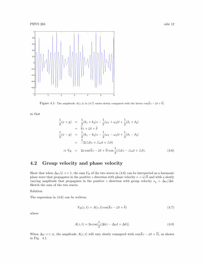
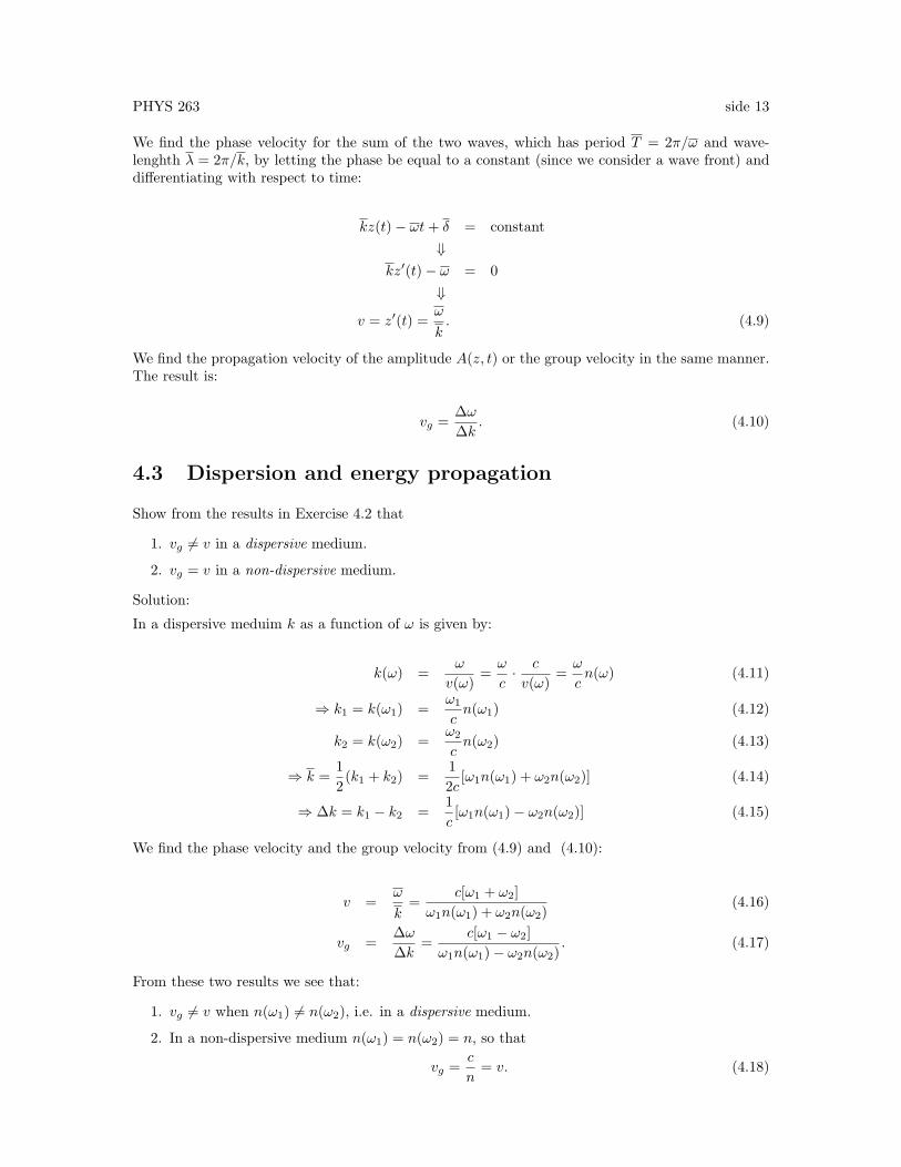
Figure 4.1: The amplitude A(z, t) in (4.7) varies slowly compared with the factor cos(kz − ωt + δ).
so that
12(x+ y) =
12(k1 + k2)z −
12(ω1 + ω2)t+
12(δ1 + δ2)
= kz + ωt+ δ12(x− y) =
12(k1 − k2)z −
12(ω1 − ω2)t+
12(δ1 − δ2)
=12(4kz +4ωt+4δ)
⇒ VR = 2a cos(kz − ωt+ δ) cos12(4kz −4ωt+4δ). (4.6)
4.2 Group velocity and phase velocity
Show that when ∆ω/ω << 1, the sum VR of the two waves in (4.6) can be interpreted as a harmonicplane wave that propagates in the positive z direction with phase velocity v = ω/k and with a slowlyvarying amplitude that propagates in the positive z direction with group velocity vg = ∆ω/∆k.Sketch the sum of the two waves.
Solution:
The expression in (4.6) can be written:
VR(z, t) = A(z, t) cos(kz − ωt+ δ) (4.7)
where
A(z, t) = 2a cos[12(∆kz −∆ωt+ ∆δ)]. (4.8)
When ∆ω << ω, the amplitude A(z, t) will vary slowly comapred with cos(kz − ωt + δ), as shownin Fig. 4.1.
PHYS 263 side 13
We find the phase velocity for the sum of the two waves, which has period T = 2π/ω and wave-lenghth λ = 2π/k, by letting the phase be equal to a constant (since we consider a wave front) anddifferentiating with respect to time:
kz(t)− ωt+ δ = constant⇓
kz′(t)− ω = 0⇓
v = z′(t) =ω
k. (4.9)
We find the propagation velocity of the amplitude A(z, t) or the group velocity in the same manner.The result is:
vg =∆ω∆k
. (4.10)
4.3 Dispersion and energy propagation
Show from the results in Exercise 4.2 that
1. vg 6= v in a dispersive medium.
2. vg = v in a non-dispersive medium.
Solution:
In a dispersive meduim k as a function of ω is given by:
k(ω) =ω
v(ω)=ω
c· c
v(ω)=ω
cn(ω) (4.11)
⇒ k1 = k(ω1) =ω1
cn(ω1) (4.12)
k2 = k(ω2) =ω2
cn(ω2) (4.13)
⇒ k =12(k1 + k2) =
12c
[ω1n(ω1) + ω2n(ω2)] (4.14)
⇒ ∆k = k1 − k2 =1c[ω1n(ω1)− ω2n(ω2)] (4.15)
We find the phase velocity and the group velocity from (4.9) and (4.10):
v =ω
k=
c[ω1 + ω2]ω1n(ω1) + ω2n(ω2)
(4.16)
vg =∆ω∆k
=c[ω1 − ω2]
ω1n(ω1)− ω2n(ω2). (4.17)
From these two results we see that:
1. vg 6= v when n(ω1) 6= n(ω2), i.e. in a dispersive medium.
2. In a non-dispersive medium n(ω1) = n(ω2) = n, so that
vg =c
n= v. (4.18)
PHYS 263 side 14
Chapter 5
Connection between group velocity,phase velocity, and refractive index
5.1 Group velocity as a function of phase velocity and re-fractive index
Show that the group velocity vg can be expressed in terms of the phase velocity v and the refractiveindex n(ω) in the following manner:
1vg
=1v
+ω
c
dn(ω)dω
. (5.1)
Solution:
vg =dω
dk⇒ 1
vg=dk
dω(5.2)
k =ω
v=ω
c
c
v=ω
cn =
ω
cn(ω)
⇒ 1vg
=d
dω(ω
cn(ω)) =
n(ω)c
+ω
c
dn
dω
⇒ 1vg
=1v
+ω
c
dn
dω. (5.3)
5.2 The group velocity is less than the speed of light in vac-uum
Given that
n =√
1− B
ω2 − ω02
; B > 0 (5.4)
show that vg < c when ω < ω0.
PHYS 263 side 15
Solution:
n2 = 1− B
ω2 − ω02
; B > 0 (5.5)
⇒ 2ndn
dω=
B · 2ω(ω2 − ω0
2)2
⇒ dn
dω=
Bω
n(ω2 − ω02)2
. (5.6)
We substitute this result in (5.3) to obtain
⇒ 1vg
=1v
+ω
c
Bω
n(ω2 − ω02)2
⇒ c
vg= n+
Bω2
n(ω2 − ω02)2
. (5.7)
Because B > 0, we see that cvg> n. But when ω < ω0, it follows from (5.5) that n > 1. Thus, we
have cvg> 1 or vg < c, which was to be proven.
PHYS 263 side 16
Chapter 6
Propagation in a dispersivemedium
Consider a polychromatic plane wave that propagates in the z direction in a dispersive medium, sothat
u(z, t) =12π
∫ ∞
−∞u(0, ω)ei[k(ω)z−ωt]dω. (6.1)
It follows from (6.1) that in the plane z = 0
u(0, t) =12π
∫ ∞
−∞u(0, ω)e−iωtdω (6.2)
so that
u(0, ω) =∫ ∞
−∞u(0, t)eiωtdt (6.3)
where u(0, ω) is the frequency spectrum of the plane wave in the plane z = 0. Let the frequencyspectrum u(0, ω) have its maximum value at ω = ω0, and let u(0, ω) fall off rapidly from this value,so that we may represent k(ω) by the first two terms in a Taylor series around ω0:
k(ω) = k(ω0) +dk
dω
∣∣∣∣ω=ω0
(ω − ω0). (6.4)
6.1 Propagation of a quasi-monochromatic wave
Show that when we neglect terms of higher order than those retained in (6.4), we can express u(z, t)in (6.1) as follows:
u(z, t) ≈ eiω0z
(1
v0− 1
vg0
)u
(0,− z
vg0+ t
)(6.5)
where
v0 =ω0
k(ω0); vg0 =
dω
dk
∣∣∣∣ω=ω0
. (6.6)
PHYS 263 side 17
Solution:
By using the information given in the exercise, we may write:
k(ω) = k(ω0) +
(1dωdk
)∣∣∣∣∣ω=ω0
(ω − ω0) =ω0
v0− ω0
vg0+
ω
vg0(6.7)
so that
k(ω)z − ωt ≈ ω0z
(1v0− 1vg0
)+ ω
(z
vg0− t
)(6.8)
which upon substitution in (6.1) gives:
u(z, t) ≈ eiω0z
(1
v0− 1
vg0
)12π
∫ ∞
−∞u(0, ω)e−iω
(− z
vg0+t)dω. (6.9)
Because of the Fourier transform relation given in (6.2), (6.9) becomes
u(z, t) ≈ eiω0z
(1
v0− 1
vg0
)u
(0,− z
vg0+ t
). (6.10)
6.2 The shape and speed of the wave
Give a physical interpretation of the result in (6.10).
Solution:
v0 and vg0 are the phase velocity and group velocity, respectively, at angular frequency ω0. Theresult in (6.10) shows that when u(0, ω) has its maximum value at ω0 and falls off rapidly from itsmaximum value of u(0, ω0), then, except for a phase factor, u(t) will not change its form, and u(t)will propagate at the group velocity.
6.3 Alternative way to proceed
Show that the same result as in (6.10) can be obtained by considering
u(z, t) =12π
∫ ∞
−∞u(0, ω)ei
zc f(ω)dω (6.11)
where
f(ω) = ω[n(ω)− θ] ; θ =ct
z(6.12)
and expanding f(ω) in a Taylor series around ω0 to the first order, i.e.
f(ω) = f(ω0) + f ′(ω0)(ω − ω0). (6.13)

PHYS 263 side 18
Solution:
f(ω) = ω[n(ω)− θ] ; θ =ct
z⇓
f ′(ω) = n(ω)− θ + ωdn
dω= n(ω)− θ + ωn′(ω) (6.14)
Thus, we havef ′(ω0) = n(ω0)− θ + ω0n
′(ω0) (6.15)
so that (6.13) gives
f(ω) = f(ω0) + f ′(ω0)(ω − ω0)= ω0[n(ω0)− θ] + [n(ω0)− θ + ω0n
′(ω0)](ω − ω0)= −ω2
0n′(ω0) + ω[n(ω0)− θ + ω0n
′(ω0)]. (6.16)
Further, we have:
vg =dω
dk⇒ 1
vg=
dk
dω=
d
dω
(ωcn(ω)
)=n(ω)c
+ω
cn′(ω)
⇒ 1vg0
=n(ω0)c
+ω0
cn′(ω0) =
1v0
+ω0
cn′(ω0). (6.17)
from which we obtain:
ω0n′(ω0) = c
[1vg0
− 1v0
]; vg0 = vg(ω0) ; v0 = v(ω0). (6.18)
By combining (6.16) with (6.18), we get
f(ω) = −ω20
c
ω0[
1vg0
− 1v0
] + ω
{n(ω0)− θ + ω0
c
ω0[
1vg0
− 1v0
]}
(6.19)
= −ω0c[1vg0
− 1v0
] + ω
{n(ω0)− θ + c[
1vg0
− 1v0
]}. (6.20)
By substituting the expression for f(ω) in (6.20) into the expression for u(z, t) in (6.11), we get
u(z, t) = eizω0[
1v0− 1
vg0] 12π
∫ ∞
−∞u(0, ω)eiω
zc
{c
v0− ct
z +c[ 1vg0
− 1v0
]}dω
= eizω0[
1v0− 1
vg0] 12π
∫ ∞
−∞u(0, ω)e−iω[− z
vg0+t]dω. (6.21)
Finally, we get from (6.21) and 6.2
u(z, t) = eizω0[
1v0− 1
vg0]u
(0,− z
vg0+ t
). (6.22)
PHYS 263 side 19
Chapter 7
Polarisation and rotation ofco-ordinate system
7.1 Maximum and minimum values
Show that the ellipse (Eq. (15), page 25 in Born and Wolf [?]):
x2
a12
+y2
a22− 2
x
a1
y
a2cos δ = sin2 δ (7.1)
has the following maximum and minimum values:
ymaks = a2 for x = a1 cos δymin = −a2 for x = −a1 cos δxmaks = a1 for y = a2 cos δxmin = −a1 for y = −a2 cos δ. (7.2)
Solution:
We consider y as a function of x and define the function F (x, y(x)) as follows:
F (x, y(x)) = 0 ; F (x, y(x)) =y2
a22
+x2
a12− 2
x
a1
y
a2cos δ − sin2 δ. (7.3)
By implicit differentiation (as in chapter 13.7 in [?]) we have:
∂F
∂x+∂F
∂y
dy
dx= 0 ⇒ dy
dx= −
∂F∂x∂F∂y
. (7.4)
Thus, we get
dx
dy= 0 for y =
∂F
∂y= 0. (7.5)

PHYS 263 side 20
Further, we have that ∂F∂y = 2a2
a1x cos δ, implying that x has a maximum or minimum value for
y = a2a1x cos δ. By substituting this in (7.1), we find that the minimum or maximum value x2
e for x2
is given by:
xe2
a12
+[a2a1xe cos δ]2
a22
− 2xea1
[a2a1xe cos δ
]a2
cos δ = sin2 δ (7.6)
which gives
xe2 = a1
2 (7.7)
or
xmaks = a1 for y = a2 cos δxmin = −a1 for y = −a2 cos δ. (7.8)
We can find the minimum and maximum values for y by solving (7.1) with respect to x2 and thendifferentiating with respect to y and following the same procedure as above. But due to the symmetryin (7.1) with respect to the exchange of x and y as well as of a1 and a2, we obtain the desired resultby making these exchanges in the result given above:
ymaks = a2 for x = a1 cos δymin = −a2 for x = −a1 cos δ.
(7.9)
7.2 Rotation of co-ordinate system
Show that by rotating the co-ordinate system an angle Ψ, so that
x = ξ cos Ψ− η sinΨ ; y = ξ sinΨ + η cos Ψ (7.10)
the coefficients in front of the ξη term in the equation obtained from (7.1) as a result of this rotationwill disappear if Ψ satisfies the relation
tan(2Ψ) = tan(2α) cos δ ; tanα =a2
a1. (7.11)
Solution:
We write (7.1) in the form:
a22x2 + a1
2y2 − 2a1a2xy cos δ = a12a2
2 sin2 δ. (7.12)
By letting
x = ξ cos Ψ− η sinΨ ; y = ξ sinΨ + η cos Ψ (7.13)
we get
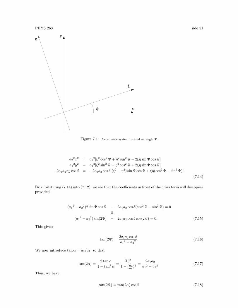
PHYS 263 side 21
η
ψ
y
x
ξ
Figure 7.1: Co-ordinate system rotated an angle Ψ.
a22x2 = a2
2[ξ2 cos2 Ψ + η2 sin2 Ψ− 2ξη sinΨ cos Ψ]a1
2y2 = a12[ξ2 sin2 Ψ + η2 cos2 Ψ + 2ξη sinΨ cos Ψ]
−2a1a2xy cos δ = −2a1a2 cos δ[(ξ2 − η2) sinΨ cos Ψ + ξη(cos2 Ψ− sin2 Ψ)].(7.14)
By substituting (7.14) into (7.12), we see that the coefficients in front of the cross term will disappearprovided
(a12 − a2
2)2 sinΨ cos Ψ − 2a1a2 cos δ(cos2 Ψ− sin2 Ψ) = 0⇓
(a12 − a2
2) sin(2Ψ) − 2a1a2 cos δ cos(2Ψ) = 0. (7.15)
This gives:
tan(2Ψ) =2a1a2 cos δa1
2 − a22. (7.16)
We now introduce tanα = a2/a1, so that
tan(2α) =2 tanα
1− tan2 α=
2a2a1
1− (a2a1
)2=
2a1a2
a12 − a2
2. (7.17)
Thus, we have
tan(2Ψ) = tan(2α) cos δ. (7.18)
PHYS 263 side 22
7.3 Simplification of the expression for the ellipse
Show that in (ξ, η) co-ordinates (7.1) can be written as follows:
b2ξ2 + a2η2 = a2b2 (7.19)
where
a2 = a22 sin2 Ψ + a1
2 cos2 Ψ + 2a1a2 cos δ sinΨ cos Ψb2 = a2
2 cos2 Ψ + a12 sin2 Ψ− 2a1a2 cos δ sinΨ cos Ψ. (7.20)
Solution:
By substituting (7.14) into (7.12) and choosing Ψ such that the cross term disappears, we obtain:
ξ2[a22 cos2 Ψ + a1
2 sin2 Ψ− 2a1a2 cos δ sinΨ cos Ψ]+ η2[a2
2 sin2 Ψ + a12 cos2 Ψ + 2a1a2 cos δ sinΨ cos Ψ]
= a12a2
2 sin2 δ. (7.21)
Thus, we have
b2ξ2 + a2η2 = a12a2
2 sin2 δ (7.22)
where
b2 = a22 cos2 Ψ + a1
2 sin2 Ψ− 2a1a2 cos δ sinΨ cos Ψa2 = a2
2 sin2 Ψ + a12 cos2 Ψ + 2a1a2 cos δ sinΨ cos Ψ. (7.23)
It remains to show that a2b2 = a12a2
2 sin2 δ. By use of the formulas
cos2 Ψ =1 + cos(2Ψ)
2; sin2 Ψ =
1− cos(2Ψ)2
(7.24)
we get
2b2 = a22(1 + cos(2Ψ)) + a1
2(1− cos(2Ψ))− 2a1a2 cos δ sin(2Ψ) (7.25)
which gives
b2 =12[a2
1 + a22 +A] (7.26)
where
A = (a22 − a1
2) cos(2Ψ)− 2a1a2 cos δ sin(2Ψ). (7.27)
Similarly, we find that
a2 =12[a2
1 + a22 −A] (7.28)
PHYS 263 side 23
so that
a2b2 =14[(a2
1 + a22)
2 −A2]. (7.29)
From Exercise 7.1 we have
tan(2Ψ) =2a1a2 cos δa1
2 − a22
(7.30)
which gives
sin(2Ψ) =2a1a2 cos δ√
B; cos(2Ψ) =
a21 − a2
2√B
(7.31)
where
B = (a12 − a2
2)2 + (2a1a2 cos δ)2. (7.32)
By substituting (7.31) into (7.27), we obtain
A = (a22 − a1
2)a1
2 − a22
√B
− 2a1a2 cos δ2a1a2 cos δ√
B
= − B√B
= −√B (7.33)
which upon substitution in (7.29) gives:
a2b2 =14[(a1
2 + a22)2 −B]
=14[(a1
2 + a22)2 − (a1
2 − a22)2 − (2a1a2 cos δ)2]
=14[4a1
2a22(1− cos2 δ)]
= a12a2
2 sin2 δ. (7.34)
Substitution of this result in (7.22) gives:
b2ξ2 + a2η2 = a2b2 (7.35)
where a2 and b2 are given in (7.23).
PHYS 263 side 24
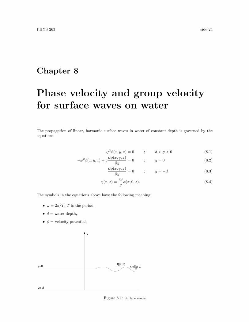
Chapter 8
Phase velocity and group velocityfor surface waves on water
The propagation of linear, harmonic surface waves in water of constant depth is governed by theequations
52φ(x, y, z) = 0 ; d < y < 0 (8.1)
−ω2φ(x, y, z) + g∂φ(x, y, z)
∂y= 0 ; y = 0 (8.2)
∂φ(x, y, z)∂y
= 0 ; y = −d (8.3)
η(x, z) =iω
gφ(x, 0, z). (8.4)
The symbols in the equations above have the following meaning:
• ω = 2π/T ; T is the period,
• d = water depth,
• φ = velocity potential,
y=0
y=-d
x eller z
y
η(x,z)
Figure 8.1: Surface waves
PHYS 263 side 25
• g = acceleration of gravity, and
• η = displacement of the water surface from the position y = 0, which is its position at rest.
The velocity v of a water ”particle” is given as
v = 5φ. (8.5)
8.1 Separation of variables
Use separation of variables to find the solution of (8.1). Thus, express φ as a product
φ = A(y)B(x, z) (8.6)
where A only depends on y and B only depends on x and z, and show by substitution into (8.1)that
∂2A(y)∂2y
− k2A(y) = 0 (8.7)(∂2
∂x2+
∂2
∂z2+ k2
)B(x, z) = 0 (8.8)
where k2 is a separation constant.
Solution:
52φ =(∂2
∂x2+
∂2
∂y2+
∂2
∂z2
)A(y)B(x, z)
= A(y)[∂2
∂x2+
∂2
∂y2
]B(x, z) +B(x, z)
∂2
∂y2A(y) = 0
⇒ 1A(y)
∂2A(y)∂y2
= − 1B(x, z)
[∂2
∂x2+
∂2
∂y2
]B(x, z) = k2 (8.9)
where k2 (the separation constant) must be a constant because the left-hand side of the equationdepends on y only, while the right-hand side depends on x and z. Thus, both sides must be equalto the same constant, which we here have denoted by k2. Equation (8.9) gives the following twoequations:
(∂2
∂y2− k2)A(y) = 0 (8.10)
(∂2
∂x2+
∂2
∂y2+ k2)B(x, z) = 0. (8.11)
PHYS 263 side 26
8.2 Dispersion relation
Show that
A(y) = C cosh[k(y + d)] ; C = constant (8.12)
satisfies (8.3) and (8.10). Substitute this solution into (8.2) and show that the dispersion relation,i.e. the relation between ω and k is as follows:
ω2 = gk tanh(kd). (8.13)
Solution:
First we show that A(y) satisfies (8.10). From (8.6) we have for φ:
φ = A(y)B(x, z) = C cosh[k(y + d)] ·B(x, z)
⇒ ∂φ
∂y= C sinh[k(y + d)]B(x, z)|y=−d = 0 (8.14)
which was to be proven.
The general solution of (8.10) is
A(y) = C1eky + C2e
−ky. (8.15)
By choosing
C1 =12Cekd og C2 =
12Ce−kd (8.16)
we get
A(y) =12C(ek(d+y) + e−k(d+y)
)= C cosh[k(y + d). (8.17)
Since A′′(y) = k2A(y), which follows by differentiating the expression above twice, we see that (8.10)is satisfied. By substitution of the expression for φ above into (8.2), we get
[−ω2B(x, z) · cosh[k(y + d)] + gB(x, z) · Ck sinh[k(y + d)]
]∣∣y=0
= 0 (8.18)
which gives
−ω2 cosh(kd) + gk sinh(kd) = 0 (8.19)
or
ω2 = gk tanh(kd). (8.20)

PHYS 263 side 27
8.3 Phase velocity and group velocity
Find the phase velocity and the group velocity.
Solution:
Phase velocity:
v =ω
k=
1k
√gk tanh(kd)
⇒ v =√g
ktanh(kd). (8.21)
We obtain an alternative expression by writing
v =ω
k=ω2
ωk=gk tanh(kd)
ωk
=g tanh(kd)
ω
=gT tanh(kd)
2π. (8.22)
Differentiating (8.20), we get
2ωdω
dk= g
[tanh(kd) + k
1cosh2(kd)
d
](8.23)
which gives the group velocity
vg =dω
dk=
12g
ω
[tanh(kd) +
kd
cosh2(kd)
]. (8.24)
8.4 The phase velocity of surface waves in water of infinitedepth
Show that when the water depth increases, so that kd→∞, then the phase velocity approaches thefollowing limiting value
v → v0 =g
2πT (8.25)
whereas the group velocity approaches the limiting value
vg → vg0 =12v0. (8.26)
Solution:
When kd→∞, we have
PHYS 263 side 28
limkd→∞
tanh(kd) = 1 (8.27)
limkd→∞
kd
cosh2(kd)= 0 (8.28)
so that we get
v = v0 =√
g
k0=g
ω(8.29)
vg = vg0 =12g
ω=
12v0. (8.30)
Since ω = 2πT , we get v0 = g
2πT , which was to be proven.
8.5 The phase velocity of surface waves in water of finitedepth
Show that vg < v also when the depth is finite.
Solution:
From (8.24) we have
vg =12g
ω
[tanh(kd) +
kd
cosh2(kd)
]=
12g
ωtanh(kd)
1 +kd
sinh(kd)cosh(kd) cosh2(kd)
=
12g
ωtanh(kd)[1 +
2kd2 sinh(kd) cosh(kd)
]. (8.31)
Since [cf. (8.20)]
v2 =ω2
k2=g
ktanh(kd) (8.32)
we have
g
ωtanh(kd) =
k
ω
g
ktanh(kd) =
v2
ω/k= v. (8.33)
Also, 2 sinh(x) cosh(x) = sinh(2x), so that we get
vg =12v
[1 +
1sinh(x)x
]; x = 2kd. (8.34)
Since sinh(x)/x > 1, as shown below:
sinh(x)x
=1x·∞∑n=0
x2n+1
(2n+ 1)!= 1 +
∞∑n=1
x2n
(2n+ 1)!> 1 (8.35)
we find that vg < v, which was to be proven.
PHYS 263 side 29
8.6 The refractive index
The refractive index for water waves is defined as
n =v0v
(8.36)
where v0 is the phase velocity in water of infinite depth given by (8.30). Note the similarity withlight waves, in which case v0 corresponds to the speed of light in vacuum. Show that n can beexpressed as
n = coth(nk0d) (8.37)
where
k0 =ω
v0=ω2
g=
4π2
gT 2. (8.38)
(Hint: Use that k = ωv = ω
v0v0v = k0n.)
Determine n numerically for T = 12 s and d = 100 m and for T = 12 s and d = 25 m.
Solution:
n =v0v
=
√gk0√
gk tanh kd
. (8.39)
With k = k0n we get
n2 =gk0
gk tanh kd
=n
tanh(nk0d)(8.40)
or
n = coth(nk0d) (8.41)
which was to be proven.
To determine n numerically from the transcendental equation in (8.41), we let x = n and α = k0d,so that (8.41) becomes
g(x) = x− coth(αx) =x
tanh(αx)f(x) = 0 (8.42)
which implies that
f(x) = tanh(αx)− 1x
= 0. (8.43)
We may use Newton’s iterative method, illustrated in Fig. 8.2, to solve (8.43). Starting with
x = x1, we see from Fig. 8.2 that
f ′(x1) =f(x1)x1 − x2
(8.44)
or
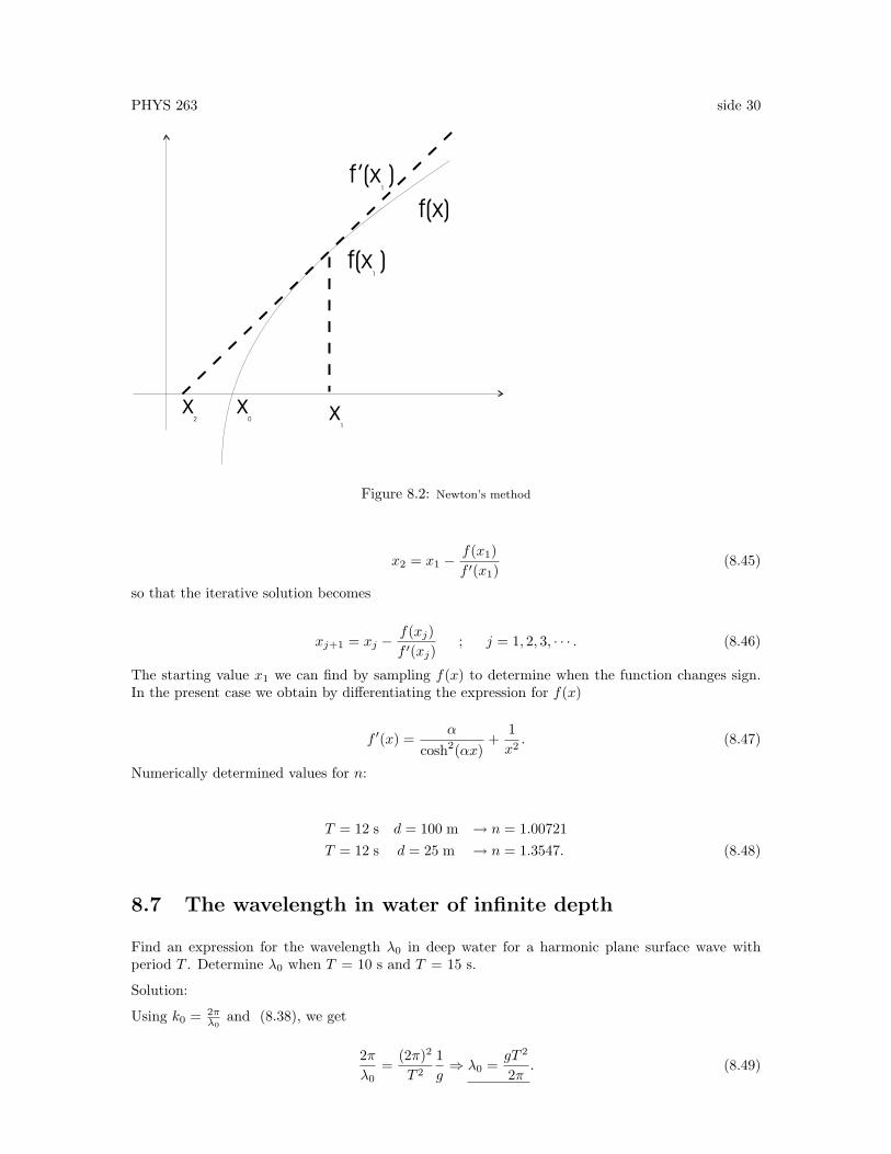
PHYS 263 side 30
Figure 8.2: Newton’s method
x2 = x1 −f(x1)f ′(x1)
(8.45)
so that the iterative solution becomes
xj+1 = xj −f(xj)f ′(xj)
; j = 1, 2, 3, · · · . (8.46)
The starting value x1 we can find by sampling f(x) to determine when the function changes sign.In the present case we obtain by differentiating the expression for f(x)
f ′(x) =α
cosh2(αx)+
1x2. (8.47)
Numerically determined values for n:
T = 12 s d = 100 m → n = 1.00721T = 12 s d = 25 m → n = 1.3547. (8.48)
8.7 The wavelength in water of infinite depth
Find an expression for the wavelength λ0 in deep water for a harmonic plane surface wave withperiod T . Determine λ0 when T = 10 s and T = 15 s.
Solution:
Using k0 = 2πλ0
and (8.38), we get
2πλ0
=(2π)2
T 2
1g⇒ λ0 =
gT 2
2π. (8.49)

PHYS 263 side 31
T = 10s ⇒ λ0 =1
6.28· 9.81
ms2· 100s2 = 156m (8.50)
T = 15s ⇒ λ0 =1
6.28· 9.81
ms2· 225s2 = 351.3m. (8.51)
8.8 The wavelength in water of finite depth
Determine the wavelength λ for the wave in water of constant depth d expressed in terms of λ0, d,and the refractive index n. Compute λ for T = 12 s and d = 100 m and for T = 12 s and d = 25 m.
Solution:
λ =λ0
n=
λ0
coth( 2πndλ0
). (8.52)
For T = 12 s and d = 100 m, we have that n = 1.00721, so that
λ =λ0
n=gT 2
2πn=
9.81 · (12)2
6.28 · 1.00721=
224.831.00721
= 223.22 m (8.53)
and for T = 12 s and d = 25 m, we have n = 1.3547, and hence
λ =λ0
n=gT 2
2πn=
9.81 · (12)2
6.28 · 1.3547=
224.831.3547
= 165.96 m. (8.54)
8.9 Refraction of waves that propagate towards a beach
A plane wave with a period T = 12 s propagates from infinitely deep water towards an area with aconstant finite depth of d = 25 m. The angle of incidence θi (see Fig. 8.3) is 30◦. Use Snell′s lawfor water waves (n1 sin θi = n2 sin θt) to determine the angle of refraction θt.
Solution:
For T = 12 s and d = 25 m, we have n = 1.3547, and hence
sin θt =sin θi
n2=
sin 30◦
1.3547= 0.369 ⇒ θt = 21.66◦. (8.55)
This change of direction explains why a wave that travels towards a beach – irrespective of itsdirection of incidence – changes its direction such that the wave crest finally becomes parallel to thebeach.
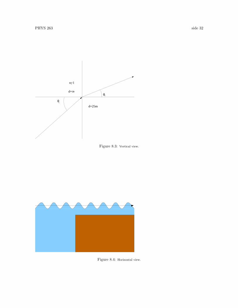
PHYS 263 side 32
θi
8
θt
d=25m
n=11
d=
Figure 8.3: Vertical view.
Figure 8.4: Horisontal view.
PHYS 263 side 33
Chapter 9
Fresnel’s formulas
9.1 Rewriting of Fresnel’s formulas
Use Snell’s law to show that the Fresnel formulas for reflection and transmission
TTM =2n1 cos θi
n2 cos θi + n1 cos θt; RTM =
n2 cos θi − n1 cos θt
n2 cos θi + n1 cos θt
TTE =2n1 cos θi
n1 cos θi + n2 cos θt; RTE =
n1 cos θi − n2 cos θt
n1 cos θi + n2 cos θt(9.1)
can be expressed as follows:
TTM =2 sin θt cos θi
sin(θi + θt) cos(θi − θt); RTM =
tan(θi − θt)tan(θi+ θt)
TTE =2 sin θt cos θi
sin(θi + θt); RTE = − sin(θi − θt)
sin(θi + θt). (9.2)
Solution:
We start by considering the expression for TTM , and we use Snell’s law n1 sin θi = n2 sin θt to rewriteit as follows
TTM =2n1 cos θi
n2 cos θi + n1 cos θt
=2n1 sin θi cos θi
n2 sin θi cos θi + n1 sin θi cos θt
=2n2 sin θt cos θi
n2 sin θi cos θi + n2 sin θt cos θt
=2 sin θt cos θi
sin θi cos θi + sin θt cos θt. (9.3)
Next, we show that sinx cosx± sin y cos y = sin(x± y) cos(x∓ y):
PHYS 263 side 34
sin(x± y) cos(x∓ y) = (sinx cos y ± cosx sin y)(cosx cos y ± sinx sin y)= sinx cosx(cos2 y + sin2 y)± sin y cos y(sin2x+ cos2 x)= sinx cosx± sin y cos y.
(9.4)
Using (9.4), we may rewrite (9.2) as follows
TTM =2 sin θt cos θi
sin(θi + θt) cos(θi − θt). (9.5)
For the refelction coefficient for TM waves we have
RTM =n2 cos θi − n1 cos θt
n2 cos θi + n1 cos θt=
n2n1
cos θi − cos θtn2n1
cos θi + cos θt
=sin θi
sin θt cos θi − cos θtsin θi
sin θt cos θi + cos θt=
sin θi cos θi − sin θt cos θt
sin θi cos θi + sin θt cos θt
=sin(θi − θt) cos(θi + θt)sin(θi + θt) cos(θi − θt)
(9.6)
where we have used (9.4) in the final step. Thus, we have
RTM =tan(θi − θt)tan(θi + θt)
. (9.7)
For the transmission coefficient for TE waves we have
TTE =2n1 cos θi
n1 cos θi + n2 cos θt=
2 cos θi
cos θi + sin θi
sin θt cos θt
=2 sin θt cos θi
sin θt cos θi + cos θt sin θi
⇒ TTE =2 sin θt cos θi
sin(θi + θt). (9.8)
For the reflection coefficient for TE waves we have
RTE =n1 cos θi − n2 cos θt
n1 cos θi + n2 cos θt=
cos θi − sin θi
sin θt cos θt
cos θi + sin θi
sin θt cos θt
=sin θt cos θi − sin θi cos θt
sin θt cos θi + sin θicosθt
⇒ RTE = − sin(θi − θt)sin(θi + θt)
. (9.9)
PHYS 263 side 35
9.2 The sign of the reflection and transmission coefficients
Provided that θi and θt are real angles, determine under what circumstances TTM , RTM , TTE , andRTE are positive and negative. What physical interpretation do we associate with negative values?
Solution:
We assume θi og θt are real agles and that 0 ≤ θi < π2 ; 0 ≤ θt ≤ π
2 . Then 0 ≤ θi+θt ≤ π and hencesin(θi + θt) > 0. Further, we have that cos(θi − θt) = cos θi cos θt + sin θi sin θt > 0, and thereforeTTM og TTE are always positive. To analyse the the reflection coefficients we first assume that
n2 > n1 or θi > θt ⇒ RTE < 0
If θi + θt <π
2we have : RTM > 0
and if θi + θt >π
2: RTM < 0.
(9.10)
Next, we assume that
n2 < n1 or θi < θt ⇒ RTE > 0
If θi + θt <π
2we have : RTM < 0
and if θi + θt >π
2: RTM > 0.
(9.11)
A negative value for a reflection coefficient implies that there is a phase change of π between theincident and the reflected wave.
PHYS 263 side 36
Chapter 10
Reflectivity and transmissivity
10.1 Energy conservation for TE and TM components
From the formulas for the reflectivities and the transmissivities, given by
T TM =sin 2θi sin 2θt
sin2(θi + θt) cos2(θi − θt); RTM =
tan2(θi − θt)tan2(θi + θt)
T TE =sin 2θt sin 2θi
sin2(θi + θt); RTE = − sin2(θi − θt)
sin2(θi + θt)(10.1)
show that
T TM +RTM = 1 ; T TE +RTE = 1. (10.2)
Solution:
RTM =tan2(θi − θt)tan2(θi + θt)
=sin2(θi − θt) cos2(θi + θt)sin2(θi + θt) cos2(θi − θt)
T TM =sin 2θi sin 2θt
sin2(θi + θt) cos2(θi − θt)
⇒ RTM + T TM =sin 2θi sin 2θt + sin2(θi − θt) cos2(θi + θt)
sin2(θi + θt) cos2(θi − θt). (10.3)
Thus, we have
RTM + T TM = 1 +N
D(10.4)
where
N = sin 2θi sin 2θt +A−D
A = sin2(θi − θt) cos2(θi + θt)D = sin2(θi + θt) cos2(θi − θt). (10.5)
PHYS 263 side 37
Next, we use the formula sinx cosx± sin y cos y = sin(x± y) cos(x∓ y) to obtain
A = sin2(θi − θt) cos2(θi + θt) = (sin θi cos θi − sin θt cos θt)2
D = sin2(θi + θt) cos2(θi − θt) = (sin θi cos θi + sin θt cos θt)2
⇒ A−D = −4 sin θi cos θi sin θt cos θt = − sin 2θi sin 2θt (10.6)
which shows that N = 0, and hence that
T TM +RTM = 1 (10.7)
which was to be proven. For TE polarisation we have
RTE =sin2(θi − θt)sin2(θi + θt)
T TE =sin 2θt sin 2θi
sin2(θi + θt)(10.8)
RTE + T TE = 1 +N
D(10.9)
where in this case
N = sin 2θi sin 2θt +A−D
A = sin2(θi − θt) = (sin θi cos θt − sin θt cos θi)2
D = sin2(θi + θt) = (sin θi cos θt + sin θt cos θi)2
⇒ A−D = −4 sin θi cos θt sin θt cos θi = − sin 2θi sin 2θt. (10.10)
This shows that N = 0, and hence that
T TE +RTE = 1 (10.11)
which was to be proven.
10.2 Energy conservation
Show that
T +R = 1 (10.12)
where
R = RTM cos2 αi +RTE sin2 αi
T = T TM cos2 αi + T TE sin2 αi. (10.13)
Solution:
It follows from (10.13) that
PHYS 263 side 38
R+ T = (RTM + T TM ) cos2 αi + (RTE + T TE) sin2 αi (10.14)
but since
T TM +RTM = 1 (10.15)
and
T TE +RTE = 1 (10.16)
we get
R+ T = cos2 αi + sin2 αi = 1. (10.17)
PHYS 263 side 39
Chapter 11
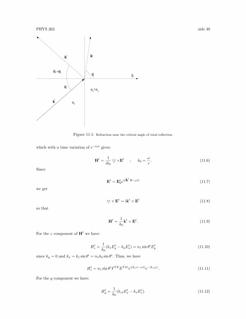
Total reflection 1
Consider a harmonic, plane wave that is incident upon a plane interface under an angle of incidenceθi that is greater than the critical angle θic, so that we have total reflection. The components of theelectric field are then given by (see section 9.3.5 of [?]):
Etx = TTMETMi cos θt ei(kxx−ωt)e−|kz2|z
Ety = TTEETEi ei(kxx−ωt)e−|kz2|z
Etz = − sin θi
n TTMETMi ei(kxx−ωt)e−|kz2|z (11.1)
where
kx = k1 sin θi =1n
ω
v2sin θi ; n =
n2
n1< 1
kz2 = k2 cos θt ; cos θt =i
n
√sin2 θi − n2. (11.2)
11.1 Transmitted magnetic field
Show from Maxwell’s equation (with µ1 = µ2 = 1)
5×Et = −1c
·Ht (11.3)
that the transmitted magnetic field Ht has the following components:
Htx = −n2 cos θtTTEETEi ei(kxx−ωt)e−|kz2|z
Hty = n2T
TMETMi ei(kxx−ωt)e−|kz2|z
Htz = n1 sin θiTTEETEi ei(kxx−ωt)e−|kz2|z. (11.4)
Solution: First we determine Ht from Maxwell’s equation
5×Et = −1c
·Ht (11.5)
PHYS 263 side 40
n <n
n
k
k
k
nr
i
=
1
2 1
^θt
θ θi
iθ
tr
Figure 11.1: Refraction near the critical angle of total reflection.
which with a time variation of e−iωt gives:
Ht =1ik0
5×Et ; k0 =ω
c. (11.6)
Since
Et = Et0ei(kt·r−ωt) (11.7)
we get
5×Et = ikt ×Et (11.8)
so that
Ht =1k0
kt ×Et. (11.9)
For the z component of Ht we have:
Htz =
1k0
(kxEty − kyEtx) = n1 sin θiEty (11.10)
since ky = 0 and kx = k1 sin θi = n1k0 sin θi. Thus, we have
Htz = n1 sin θiTTEETEiei(kxx−ωt)e−|kz2|z. (11.11)
For the y component we have:
Hty =
1k0
(kz2Etx − kxEtz). (11.12)

PHYS 263 side 41
Since k ·E = 0, and hence
Etz =−kxkz2
Etx (11.13)
we get
Hty =
1k0
(kz2E
tx − kxE
tz
)=
1k0
(kz2E
tx +
kx2
kz2Etx
)=
1k0kz2
(k2z2 + kx
2)Etx =
k22
k0kz2Etx
=k22
k2 cos θtk0TTMETMi cos θtei(kxx−ωt)e−|kz2|z = n2T
TMETMiei(kxx−ωt)e−|kz2|z.
(11.14)
For the x component we have
Htx =
1k0
(kyEtz − kz2Ety) = −kz2
k0Ety (11.15)
since ky = 0. Thus, we get
Htx = −n2 cos θtEty = −n2 cos θtTTEETEiei(kxx−ωt)e−|kz2|z. (11.16)
11.2 Transmitted Poynting vector
Show that the Poynting vector of the transmitted field
St =c
4πEt ×Ht (11.17)
has the following components:
Stx =c
16πn1 sin θie−2A {(ETEi)2
[(TTE)2e2iφ + ((TTE)∗)2e−2iφ + 2|TTE |2
]+(ETMi)2
[(TTM )2e2iφ + ((TTM )∗)2e−2iφ + 2|TTM |2
]}
(11.18)
Sty =c
4πn1 sin θie−2AETMiETEi =
{TTM [TTE ]∗
}(11.19)
Stz = − c
8πn2| cos θt|e−2A
{(ETMi)2 =
{[TTEeiφ
]2}+ (ETEi)2 =
{[TTMeiφ
]2}}(11.20)
where
A = |kz2|z ; φ = kxx− ωt. (11.21)
Solution: Since the Poynting vector is given as the vectorial product of E and B, we must use realquantities. Thus, we express the electric field components as follows
Etx = ETMie−A12[TTM cos θteiφ + (TTM cos θt)∗e−iφ
]Ety = ETEie−A
12[TTEeiφ + (TTE)∗e−iφ
]Etz = − sin θi
n ETMie−A12[TTMeiφ + (TTM )∗e−iφ
]. (11.22)
PHYS 263 side 42
Similarly, we express the magnetic field components as:
Htx = −n2E
TEie−A12[TTE cos θteiφ + (TTE cos θt)∗e−iφ
]Hty = n2E
TMie−A12[TTMeiφ + (TTM )∗e−iφ
]Htz = n1 sin θiETEie−A
12[TTEeiφ + (TTE)∗e−iφ
](11.23)
whereA = |kz2|z ; φ = kxx− ωt. (11.24)
Since cos θt is purely imaginary, (cos θt)∗ = − cos θt, so that we have
Etx = ETMie−A cos θt12[TTMeiφ − (TTM )∗e−iφ
]Ety = ETEie−A
12[TTEeiφ + (TTE)∗e−iφ
]Etz = − sin θi
n ETMie−A12[TTMeiφ + (TTM )∗e−iφ
](11.25)
and
Htx = −n2E
TEie−A cos θt12[TTEeiφ − (TTE)∗e−iφ
]Hty = n2E
TMie−A12[TTMeiφ + (TTM )∗e−iφ
]Htz = n1 sin θiETEie−A
12[TTEeiφ + (TTE)∗e−iφ
]. (11.26)
The components Stx, Sty, and Stz of the Poynting vector are given by:
Stx =c
4π[EtyH
tz − EtzH
ty]
Sty =c
4π[EtzH
tx − EtxH
tz]
Stz =c
4π[EtxH
ty − EtyH
tx]. (11.27)
Substitution from (11.25) and (11.26) into (11.27) gives
Stx =c
16πe−2An1 sin θi {(ETEi)2
[TTEeiφ + (TTE)∗e−iφ
]2+(ETMi)2
[TTMeiφ + (TTM )∗e−iφ
]2} (11.28)
Sty =c
16πe−2An1 sin θi cos θtETEiETMi {
[TTMeiφ + (TTM )∗e−iφ
] [TTEeiφ − (TTE)∗e−iφ
]−[TTMeiφ − (TTM )∗e−iφ
] [TTEeiφ + (TTE)∗e−iφ
]}
(11.29)
Stz =c
16πe−2An2 cos θt {(ETMi)2
[TTMeiφ − (TTM )∗e−iφ
] [TTMeiφ + (TTM )∗e−iφ
]−(ETEi)2
[TTEeiφ + (TTE)∗e−iφ
] [TTEeiφ − (TTE)∗e−iφ
]}.
(11.30)
Carrying out the multiplications, we get
PHYS 263 side 43
Stx = cn1 sin θi
16π e−2A {(ETEi)2[(TTE)2e2iφ + ((TTE)∗)2e−2iφ + 2|TTE |2
]+(ETMi)2
[(TTM )2e2iφ + ((TTM )∗)2e−2iφ + 2|TTM |2
]}
Sty = cn1 sin θi cos θt
8π e−2A ETMiETEi[(TTM )∗TTE − TTM (TTE)∗
]Stz = cn2 cos θt
16π e−2A {(ETMi)2[(TTM )2e2iφ − ((TTM )∗)2e−2iφ
]+(ETEi)2
[(TTE)2e2iφ − ((TTE)∗)2e−2iφ
]}.
(11.31)
This expression for Stx is equal to the one given in (11.18). To show that the expressions for Styand Stz given above are equal to those given in (11.19) and (11.20), respectively, we note thatcos θt = i| cos θt| and use the relation i(z − z∗) = −=z, which is valid for any arbitrary number z.
11.3 Time average of the Poynting vector
Show that the time-average of the z component of the Poynting vector vanishes, i.e.
< Stz >= 0, (11.32)
and that the time-averages of the x and y components are given by:
< Stx > =cn1 sin θi
8πe−2A
{|TTE |2(ETEi)2 + |TTM |2(ETEi)2
}< Sty > = −cn1 sin θi
4πe−2A| cos θt|ETMiETEi =
{(TTM )∗TTE
}. (11.33)
What is the physical explanation of this result? (Time averaging implies integration over an intervalT ′ that is much larger than the period T = 2π
ω , i.e. < St >= 12T ′
∫ T ′−T ′ S
tdt, where T ′ >> T .)
Solution: Because
12T ′
∫ T ′
−T ′e±2iωtdt =
sin(2ωT ′)4π
(T
T ′) (11.34)
terms in (11.31) that include e±2iφ will disappear on time averaging over an interval such thatT ′ >> T . Thus, we have
< Stz > = 0
< Stx > =cn1 sin θi
8πe−2A((ETEi)2|TTE |2 + (ETMi)2|TTM |2)
< Sty > = −cn1 sin θi| cos θt|4π
e−2AETMiETEi={(TTM )∗TTE}. (11.35)
This means that the time average of the energy flux is zero in the z direction. The energy propagatesin directions parallel to the interface and in the plane of incidence as long as the polarisation is eithernormal to the plane of incidence (ETMi = 0) or parallel to the plane of incidence (ETEi = 0). Butin general we have < Sty >6= 0.

PHYS 263 side 44
Chapter 12
Fresnel’s rhomb
Fig. 12.1 shows a Fresnel’s rhomb, which can be used to produce circularly polarised light fromlinearly polarised light or vice versa. The required phase difference of δ = 90◦ can be obtainedthrough two successive total reflections, each introducing a phase difference of 45◦. For a singletotal reflection the phase difference δ is given by the fomula
tanδ
2=
cos θi√
sin2 θi − n2
sin2 θi(12.1)
where θi is the angle of incidence and n = n2n1< 1.
12.1 Solution for sin θi.
Solve (12.1) with respect to sin θi, and show that
sin θi =
n2 + 1±√
(n2 + 1)2 − 4n2(1 + tan2 δ2 )
2(tan2 δ2 + 1)
12
. (12.2)
Solution: From (12.1 we get
sin4 θi tan2 δ
2= (1− sin2 θi)(sin2 θi − n2)
⇒ 0 = sin4 θi(tan2 δ
2+ 1)− (n2 + 1) sin2 θi + n2
lineærpolarisert lys
sirkulærpolarisert lys
n
n <nθ θ
θi
i
i 1
2 1
Figure 12.1: Fresnel’s rhomb
PHYS 263 side 45
⇒ sin2 θi =n2 + 1±
√(n2 + 1)2 − 4n2(1 + tan2 δ
2 )
2(tan2 δ2 + 1)
⇒ sin θi =
n2 + 1±√
(n2 + 1)2 − 4n2(1 + tan2 δ2 )
2(tan2 δ2 + 1)
12
. (12.3)
12.2 Phase difference of 45◦, n = 1/1.52 = 0.6579
For n21 = 1n = 1.52 determine those angles of incidence which give a phase difference of 45◦.
Solution: When n12 = 1n = 1.52 and δ
2 = 22.5◦, we get by substitution into (12.3):
sin θi+ = 0.81371 ⇒ θi+ = 55.45752◦
sin θi− = 0.73790 ⇒ θi− = 47.55312◦. (12.4)
12.3 Phase difference of 45◦, n = 1/1.49 = 0.6711
Repeat the task in exercise 12.2 for n21 = 1.49, and explain the result.
Solution: For n21 = 1.49 the expression inside the square root in (12.3) becomes negative. Thismeans that in order to obtain a phase difference of 45◦ in one single total reflection, n21 must belarger than 1.49.
12.4 Maximum phase difference
Show from (12.1) that δ has a maximum value δm for θi = θim given by
sin2 θim =2n2
1 + n2(12.5)
and that δm is given by:
tanδm2
=1− n2
2n. (12.6)
Solution: From (12.1) we see that δ = 0 when θi = θic (critical angle of incidence) and θi = π/2(grazing incidence). Between tese two angles there is an angle of incidence θi = θim which gives amaximum phase difference of δ = δm, where δm is determined by
dδ
dθi
∣∣∣∣θi=θim
= 0. (12.7)
Since δ = 2 arctan[tan( δ2 )], we have from (12.7)
dδ
dθi=
21 + tan2 δ
2
d
dθi(tan
δ
2) = 0. (12.8)

PHYS 263 side 46
This means that
d
dθi(tan
δ
2) = 0 ⇒ d
dθi
[cos θi
√sin2 θi − n2
sin2 θi
]= 0
⇒sin2 θi[− sin θi
√(...) + cos θi sin θ
i cos θi√(...)
]− cos θi√
(...)2 sin θi cos θi
sin4 θi= 0.
(12.9)
We multiply the last result by√
sin2 θi − n2 sin3 θi to obtain
− sin2 θi(sin2 θi − n2) + sin2 θi cos2 θi − 2 cos2 θi(sin2 θi − n2) = 0⇓
−(sin2 θi + cos2 θi)(sin2 θi − n2) + sin2 θi cos2 θi − cos2 θi(sin2 θi − n2) = 0⇓
− sin2 θi + n2 + n2(1− sin2 θi) = 0⇓
2n2 − (1 + n2) sin2 θi = 0(12.10)
so that dδdθi
∣∣θi=θim = 0 gives:
sin2 θim =2n2
1 + n2
cos2 θim = 1− 2n2
1 + n2=
1− n2
1 + n2. (12.11)
By substitution of this result into (12.1), we get
tanδm2
=√
1− n2
√1 + n2
√2n2
1+n2 − n2
2n2
1+n2
=1− n2
2n. (12.12)
12.5 Phase differences of 45◦ and 90◦
What minimum value of n12 = 1n is required to obtain a phase difference of
1. 90◦ or
2. 45◦?
Solution: From Exercise (12.4) we have that tan δ2 ≤ tan δm
2 = 1−n2
2n , from wich it follows that:
n2 + 2n tanδ
2− 1 ≤ 0
⇓
(n2 + tanδ
2)2 ≤ 1 + tan2 δ
2
PHYS 263 side 47
⇓
n ≤√
1 + tan2 δ
2− tan
δ
2⇓
n12 =1n
≥ 1√1 + tan2 δ
2 − tan δ2
. (12.13)
1. δ = 90◦ ⇒ δ2 = 45◦ and tan δ
2 = 1 so that
n21 ≥1√
2− 1=√
2 + 1 = 2.4142. (12.14)
2. δ = 45◦ ⇒ δ2 = 22.5◦ and tan δ
2 = 1−cos δsin δ = 1− 1
2
√2
12
√2
=√
2− 1, so that
n21 ≥1√
1 + (√
2− 1)2 − (√
2− 1)=
1
1−√
2 +√
2(2−√
2)= 1.4966. (12.15)
This result agrees with our finding in Exercise 12.3 showing that the expression inside the squareroot in (12.1) becomes negative for n12 = 1.49.

PHYS 263 side 48
Chapter 13
Total reflection 2
Consider reflection and refraction of a plane wave at a plane interface between two media, and letn2 ≤ n1, as illustrated in Fig. 13.1. From Snell’s law
n1 sin θi = n2 sin θt (13.1)
or
sin θt =sin θi
n; n =
n2
n1≤ 1 (13.2)
it follows that when θi > θic, where sin θic = n, then sin θt > 1. Thus, θt must be a complex number.Show that θt = α+ iβ, where
α =π
2
β = ln
sin θi
n−
√(sin θi
n
)2
− 1
. (13.3)
Solution: We start with
cos θt =√
1− sin2 θt =
√1− sin2 θi
n2. (13.4)
Since n < sin θi when θi > θic, we have
cos θt = iA ; A =
√(sin θi
n
)2
− 1. (13.5)
Further, we have cos θt = cos(α+ iβ) = cosα cos(iβ)− sinα sin(iβ), and since
cos(iβ) =ei(iβ) + e−i(iβ)
2=e−β + eβ
2= cosh(β)
sin(iβ) =ei(iβ) − e−i(iβ)
2i= i
e−β − eβ
2= i sinh(β) (13.6)
we getiA = cosα coshβ − i sinα sinhβ (13.7)
and hence
cosα coshβ = 0 (13.8)− sinα sinhβ = A. (13.9)
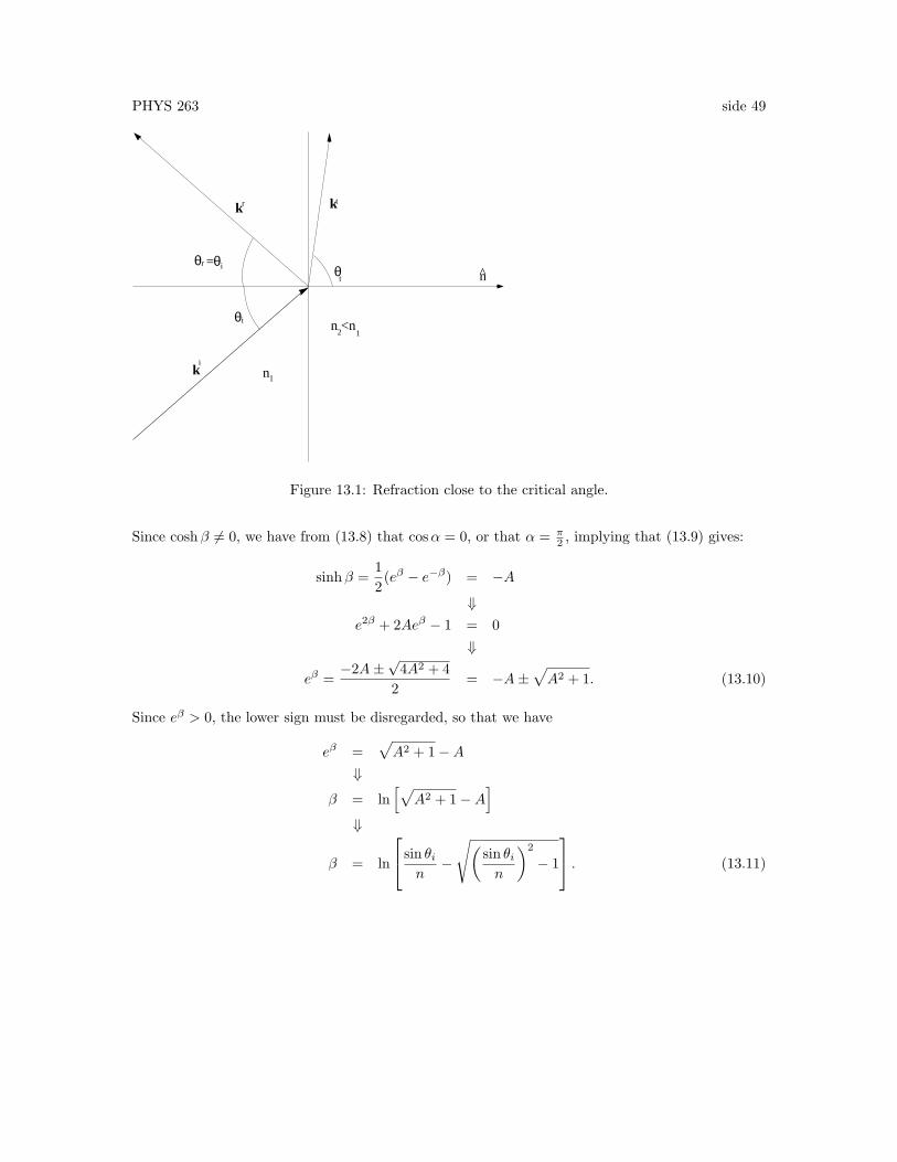
PHYS 263 side 49
n <n
n
k
k
k
nr
i
=
1
2 1
^θt
θ θi
iθ
tr
Figure 13.1: Refraction close to the critical angle.
Since coshβ 6= 0, we have from (13.8) that cosα = 0, or that α = π2 , implying that (13.9) gives:
sinhβ =12(eβ − e−β) = −A
⇓e2β + 2Aeβ − 1 = 0
⇓
eβ =−2A±
√4A2 + 4
2= −A±
√A2 + 1. (13.10)
Since eβ > 0, the lower sign must be disregarded, so that we have
eβ =√A2 + 1−A
⇓
β = ln[√
A2 + 1−A]
⇓
β = ln
sin θin
−
√(sin θin
)2
− 1
. (13.11)

PHYS 263 side 50
Part II
FYS 263 del II
PHYS 263 side 51
Chapter 14
Reflection and refraction of a planeacoustical wave
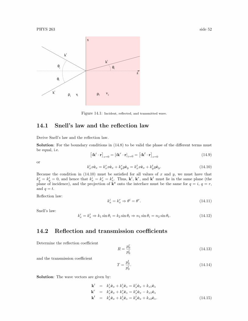
Consider two media that are separated by a plane interface and that have densities ρ1 and ρ2 andsound velocities v1 and v2. In linear acoustics the sound pressure p(r, t) is the solution of the waveequation
(52 − 1v2
∂2
∂t2)p(r, t) = 0. (14.1)
Therefore, a plane time-harmonic acoustical wave can be expressed as follows
p(r, t) = Re{p(r)e−iωt} (14.2)
wherep(r) = p0e
ik·r. (14.3)
Here the amplitude p0 is a constant. A plane harmonic pressure wave is incident upon a planeinterface as illustrated in Fig. 14.1. The incident wave pi(r) is given by
pi(r) = pi0eiki·r ; ki = kixex + kizez. (14.4)
The incident wave gives rise to a reflected plane wave and a transmitted plane wave of the samefrequency, i.e.
pr(r, t) = Re{pr(r)e−iωt}
pr(r) = pr0eikr·r ; kr = krxex + kryey + krz ez
pt(r, t) = Re{pt(r)e−iωt}
pt(r) = pt0eikt·r ; kt = ktxex + ktyey + ktzez. (14.5)
The particle velocity v is given by:v = Re{vq(r)e−iωt} (14.6)
wherevq(r) =
1iωρq
5 pq ; (q = i, r, t) (14.7)
with ρi = ρr = ρ1 and ρt = ρ2.
The boundary conditions that must be satisfied at the interface z = 0, are that the pressure p andthe component of the particle velocity normal to the interface, i.e. v · ez, both must be continuousacross the interface, i.e. [
pi + pr − pt]z=0
= 0[(vi + vr − vt) · ez
]z=0
= 0. (14.8)
PHYS 263 side 52
θ
k ρ ρ vv
rθ
θi
i
kr
kt
t
1 1 2 2
x
z
Figure 14.1: Incident, reflected, and transmitted wave.
14.1 Snell’s law and the reflection law
Derive Snell’s law and the reflection law.
Solution: For the boundary conditions in (14.8) to be valid the phase of the different terms mustbe equal, i.e. [
iki · r]z=0
= [ikr · r]z=0 =[ikt · r
]z=0
(14.9)
orkixxex = krxxex + kryyey = ktxxex + ktyyey. (14.10)
Because the condition in (14.10) must be satisfied for all values of x and y, we must have thatkry = kty = 0, and hence that kix = krx = ktx. Thus, ki, kr, and kt must lie in the same plane (theplane of incidence), and the projection of kq onto the interface must be the same for q = i, q = r,and q = t.
Reflection law:kix = krx ⇒ θi = θr. (14.11)
Snell’s law:kix = ktx ⇒ k1 sin θi = k2 sin θt ⇒ n1 sin θi = n2 sin θt. (14.12)
14.2 Reflection and transmission coefficients
Determine the reflection coefficientR =
pr0pi0
(14.13)
and the transmission coefficient
T =pt0pi0. (14.14)
Solution: The wave vectors are given by:
ki = kixex + kizez = kixex + kz1ezkr = krxex + krz ez = krxex − kz1ezkt = ktxex + ktzez = ktxex + kz2ez. (14.15)
PHYS 263 side 53
By use of the result from Exercise 14.1 we have[pi + pr − pt
]z=0
= 0 ⇒ pi0 + pr0 − pt0 = 0 (14.16)[(vi + vr − vt) · ez
]z=0
= 0 ⇒ 1iω
[kz1ρ1
(pi0 − pr0)−kz2ρ2pt0
]= 0.
(14.17)
or
1 +R = T
1−R =kz2kz1
ρ1
ρ2T (14.18)
which have the solutions
T =2ρ2kz1
ρ2kz1 + ρ1kz2(14.19)
R =ρ2kz1 − ρ1kz2ρ2kz1 + ρ1kz2
. (14.20)
14.3 Comparison with electromagnetic waves
Compare the results with the reflection and transmission coefficients for a plane electromagneticwave.
Solution: The reflection and transmission coefficients for an electromagnetic TE wave are givenby:
TTE =2µ2kz1
µ2kz1 + µ1kz2(14.21)
RTM =µ2kz1 − µ1kz2µ2kz1 + µ1kz2
. (14.22)
Thus, permeability µ plays precisely the same role here as the density ρ does in the acoustical case.The reflection and transmission coefficients for acoustical waves are the same as for electromagneticTE waves when we replace the permeability µ in the latter coefficients with the density ρ.

PHYS 263 side 54
Chapter 15
Fourier representation of a realfunction
Given the Fourier transform pair
f(t) =12π
∫ ∞
−∞f(ω)e−iωtdω
f(ω) =∫ ∞
−∞f(t)eiωtdt (15.1)
show that when f(t) is real, we can express f(t) as follows
f(t) = 2Re{
12π
∫ ∞
0
f(ω)e−iωtdω}. (15.2)
(Hint: Start by showing f∗(ω) = f(−ω).)
Solution: Since f(t) is real, it follows that f(t) = f(t)∗, and hence
f∗(ω) =∫ ∞
−∞f(t)e−iωtdt
f(−ω) =∫ ∞
−∞f(t)e−iωtdt = f∗(ω). (15.3)
In addition we have
f(t) =12π
{∫ 0
−∞f(ω)e−iωtdω +
∫ ∞
0
f(ω)e−iωtdω}. (15.4)
In the first integral we let ω → −ω, and thus we obtain∫ 0
−∞f(ω)e−iωtdω = −
∫ 0
∞f(−ω)eiωtdω =
∫ ∞
0
f∗(ω)eiωtdω =[∫ ∞
0
f(ω)e−iωtdω]∗. (15.5)
Thus, we have
f(t) =12π
{[∫ ∞
0
f(ω)e−iωtdω]∗
+∫ ∞
0
f(ω)e−iωtdω}
= 2Re{
12π
∫ ∞
0
f(ω)e−iωtdω}
(15.6)
since z + z∗ = 2Re{z} holds for any arbitrary complex number.
PHYS 263 side 55
Chapter 16
Convolution theorem,autocorrelation theorem, andParseval’s theorem
Let G(kx, ky) and g(x, y), and also H(kx, ky) and h(x, y) be Fourier transform pairs so that
A(kx, ky) =∫ ∫ ∞
−∞a(x, y)e−i(kxx+kyy)dxdy
a(x, y) =(
12π
)2 ∫ ∫ ∞
−∞A(kx, ky)ei(kxx+kyy)dkxdky (16.1)
if we let a and A stand for either g and G or h and H.
16.1 Convolution
Prove the convolution theorem(12π
)2 ∫ ∫ ∞
−∞G(kx, ky)H(kx, ky)ei(kxx+kyy)dkxdky =
∫ ∫ ∞
−∞g(x′, y′)h(x− x′, y − y′)dx′dy′.
(16.2)
Solution: We denote functions of (x, y) by lower case letters and their Fourirer transforms, whichare functions of (kx, ky) by capital letters. Thus, the Fourier transform of a function a(x, y), denotedby A(kx, ky), is defined as follows
A(kx, ky) =∫ ∫ ∞
−∞a(x, y)e−i(kxx+kyy)dxdy = F{a(x, y)}. (16.3)
The inverse Fourier transform is given by
a(x, y) =(
12π
)2 ∫ ∫ ∞
−∞A(kx, ky)ei(kxx+kyy)dkxdky = F−1{A(kx, ky)}. (16.4)
The integral
f(x, y) =∫ ∫ ∞
−∞a(x′, y′)b(x± x′, y ± y′)dx′dy′ (16.5)
PHYS 263 side 56
is a correlation or a convolution integral depending on whether we use the upper or lower sign on theright-hand side of (16.5). By expressing b(x±x′, y±y′) in (16.5) by means of its Fourier transform,we find
f(x, y) =∫ ∫ ∞
−∞a(x′, y′)
{(12π
)2 ∫ ∫ ∞
−∞B(kx, ky)ei(kx(x±x′)+ky(y±y′))dkxdky
}dx′dy′. (16.6)
We exchange the order of the integrations to obtain
f(x, y) =(
12π
)2 ∫ ∫ ∞
−∞B(kx, ky)
{∫ ∫ ∞
−∞a(x′, y′)e−i((∓kx)x′+(∓ky)y′)dx′dy′
}ei(kxx+kyy)dkxdky
(16.7)or
f(x, y) =(
12π
)2 ∫ ∫ ∞
−∞B(kx, ky)A(∓kx,∓ky)ei(kxx+kyy)dkxdky. (16.8)
By combining (16.5) and (16.8) with a = g and b = h, and using the lower sign in both equations,we obtain the convolution theorem:(
12π
)2 ∫ ∫ ∞
−∞G(kx, ky)H(kx, ky)ei(kxx+kyy)dkxdky =
∫ ∫ ∞
−∞g(x′, y′)h(x− x′, y − y′)dx′dy′.
(16.9)
16.2 Autocorrelation
Prove the autocorrelation theorem(12π
)2 ∫ ∫ ∞
−∞|G(kx, ky)|2ei(kxx+kyy)dkxdky =
∫ ∫ ∞
−∞g(x′, y′)g∗(x′ − x, y′ − y)dx′dy′. (16.10)
Solution: By choosing a = g and b = g∗(−x,−y) we obtain from (16.5) and (16.8) with the lowersign:∫ ∫ ∞
−∞g(x′, y′)g∗(x′ − x, y′ − y)dx′dy′ =
(12π
)2 ∫ ∫ ∞
−∞G(kx, ky)B(kx, ky)ei(kxx+kyy)dkxdky
(16.11)where
B(kx, ky) = F{g∗(−x,−y)} =∫ ∫ ∞
−∞g∗(−x,−y)e−i(kxx+kyy)dxdy. (16.12)
By the change of variables x→ −x and y → −y, we get:
B(kx, ky) =∫ ∫ ∞
−∞g∗(x, y)ei(kxx+kyy)dxdy =
[∫ ∫ ∞
−∞g(x, y)e−i(kxx+kyy)dxdy
]∗= [G(kx, ky)]
∗
(16.13)which upon substitution in (16.10) gives the autocorrelation theorem:(
12π
)2 ∫ ∫ ∞
−∞|G(kx, ky)|2ei(kxx+kyy)dkxdky =
∫ ∫ ∞
−∞g(x′, y′)g∗(x′ − x, y′ − y)dx′dy′. (16.14)
PHYS 263 side 57
16.3 Parseval’s theorem
Prove Parseval’s theorem(12π
)2 ∫ ∫ ∞
−∞|G(kx, ky)|2dkxdky =
∫ ∫ ∞
−∞|g(x, y)|2dxdy. (16.15)
Solution: The desired result follows from the autocorrelation theorem by setting x = y = 0in (16.14).
PHYS 263 side 58
Chapter 17
Angular-spectrum representationof a spherical wave (Weyl’sformula)
My work has always tried to unite the true with the beautiful and when I had to choose one or theother, I usually chose the beautiful. Hermann Weyl.
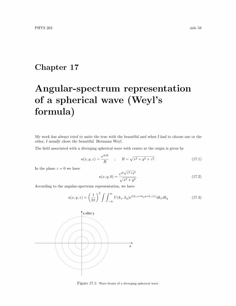
The field associated with a diverging spherical wave with centre at the origin is given by
u(x, y, z) =eikR
R; R =
√x2 + y2 + z2. (17.1)
In the plane z = 0 we have
u(x, y, 0) =eik√x2+y2√
x2 + y2. (17.2)
According to the angular-spectrum representation, we have
u(x, y, z) =(
12π
)2 ∫ ∫ ∞
−∞U(kx, ky)ei(kxx+kyy+kz|z|)dkxdky (17.3)
z
x eller y
Figure 17.1: Wave fronts of a diverging spherical wave.
PHYS 263 side 59
where the angular spectrum U(kx, ky) is given by
U(kx, ky) =∫ ∫ ∞
−∞u(x, y, 0)e−i(kxx+kyy)dxdy (17.4)
and where
kz =
√k2 − k2
x − k2y for k2 > k2
x + k2y
i√k2x + k2
y − k2 for k2 < k2x + k2
y.(17.5)
17.1 The angular spectrum
Show that the angular spectrum of a spherical wave can be written
U(kx, ky) = 2π∫ ∞
0
eiktJ0(q, t)dt (17.6)
whereq2 = k2
x + k2y. (17.7)
Solution: Substituting (17.2) in (17.4), we have
U(kx, ky) =∫ ∫ ∞
−∞
eik√x2+y2√
x2 + y2e−i(kxx+kyy)dxdy. (17.8)
We make the change of integration variables
x = r cosφy = r sinφ
dxdy = rdrdφ√x2 + y2 = r (17.9)
and let
kx = q cosψky = q sinψ√
k2x + k2
y = q (17.10)
to obtain
U(kx, ky) =∫ ∞
0
eikr∫ 2π
0
e−iqr cos(φ−ψ)dφdr
= 2π∫ ∞
0
eikrJ0(qr)dr. (17.11)
17.2 Weyl’s plane-wave expansion of a spherical wave
Use the formulas ∫ ∞
0
J0(ax) sin(bx)dx ={
0 0 < b < a1√
b2−a2 0 < a < b(17.12)
PHYS 263 side 60
and ∫ ∞
0
J0(ax) cos(bx)dx =
1√
a2−b2 0 < b < a
∞ a = b0 0 < a < b
(17.13)
to show th at U(kx, ky) in (17.6) can be written
U(kx, ky) =2πikz
. (17.14)
Use this result to find a plane-wave expansion of a spherical wave.
Solution: We start by rewriting (17.11) as follows:
U(kx, ky) = 2π{∫ ∞
0
J0(qt) cos(kt)dt+ i
∫ ∞
0
J0(qt) sin(kt)dt}. (17.15)
i) Consider first the case in which k2z > 0. Then we have k =
√k2x + k2
y + k2z =
√q2 + k2
z > q, so
that (17.12) and (17.13) give: ∫ ∞
0
J0(qt) cos(kt)dt = 0 (17.16)
∫ ∞
0
J0(qt) sin(kt)dt =1√
k2 − q2=
1√k2 − k2
x − k2y
=1kz
(17.17)
where we have used (17.5). Substitution of these results in (17.15) gives
U(kx, ky) =2πikz
. (17.18)
ii) Consider next the case in which k2z < 0. Then k =
√q2 − |kz|2 < q, so that (17.12) and (17.13)
give [cf. (17.5)]∫ ∞
0
J0(qt) cos(kt)dt =1√
q2 − k2=
1√k2x + k2
y − k2=
i
i√k2x + k2
y − k2=
i
kz(17.19)
∫ ∞
0
J0(qt) sin(kt)dt = 0 (17.20)
which upon substitution in (17.15) give
U(kx, ky) =2πikz
. (17.21)
Substitution of (17.21) in 17.3 gives
u(x, y, z) =(
12π
)2 ∫ ∫ ∞
−∞
2πikz
ei(kxx+kyy+kz|z|)dkxdky =i
2π
∫ ∫ ∞
−∞
ei(kxx+kyy+kz|z|)
kzdkxdky
(17.22)which is Weyl’s plane-wave expansion of a spherical wave exp{ikR}/R.
PHYS 263 side 61
Chapter 18
The Airy diffraction pattern
Show that ∫ 1
0
J0(vt)tdt =12
(2J1(v)v
). (18.1)
Hint: The following recursion formulas apply to Bessel functions:
d
dx
{xn+1Jn+1(x)
}= xn+1Jn(x)
d
dx
{x−nJn(x)
}= −x−nJn+1(x). (18.2)
Solution: We are to show that I =∫ 1
0J0(vt)tdt = 1
2
(2J1(v)v
). By the change of integration variable
x = vt we get:
I =1v2
∫ v
0
xJ0(x)dx. (18.3)
From the first of the two recursion relations with n = 0 it follows that: [xJ1(x)]′ = xJ0(x), so that
we get:
I =1v2
[xJ1(x)]v0 =
J1(v)v
=12
(2J1(v)v
). (18.4)
Note: limv→02J1(v)v = 1.
PHYS 263 side 62
Chapter 19
Integrated energy of the Airydiffraction pattern
19.1 Total differential for J21 (x)x
Use the recursion formulas in Exercise 18 with n = 0 to show that
J21 (x)x
= −12d
dx[J2
0 (x) + J21 (x)]. (19.1)
Solution: From ddx
{xn+1Jn+1(x)
}= xn+1Jn(x) with n = 0 we get:
d
dx{xJ1(x)} = xJ0(x) = J1(x) + xJ ′1(x). (19.2)
We multiply by J1x on both sides of (19.2) to obtain
J21 (x)x
= −J1(x)J ′1(x) + J0(x)J1(x). (19.3)
From the recurrence relation ddx {x
−nJn(x)} = −x−nJn+1(x) with n = 0 we get J ′0(x) = −J1(x),which upon substitution in (19.3) gives:
J21 (x)x
= −J1(x)J ′1(x)− J0(x)J ′0(x)
= −12d
dx[J2
0 (x) + J21 (x)]. (19.4)
19.2 Encircled energy
Fraunhofer diffraction through a circular aperture gives rise to the Airy diffraction pattern, so thatthe intensity is given by
I(v) = C
[2J1(v)v
]2(19.5)
where C is a constant and where v is a dimensionless co-ordinate given by
v = ka
z2r. (19.6)
PHYS 263 side 63
Here r is the distance from the optical axis z = 0 to the observation point. The integrated energyE(v0) inside a circle with dimensionsless radius v0 is given by the integral of I(v) over the circulararea, i.e.
E(v0) =∫ v0
0
∫ 2π
0
I(v)vdvdψ = 2π∫ v0
0
I(v)vdv. (19.7)
The ratio of E(v0) to the total energy is called the encircled energy, and is given by
L(v0) =E(v0)E(∞)
=
∫ v00
J21 (v)v dv∫∞
0
J21 (v)
v dv. (19.8)
Use the result from (19.1) and the limiting values:
J0(0) = 1J1(0) = J1(∞) = J0(∞) = 0 (19.9)
to show thatL(v0) = 1− J2
0 (v0)− J21 (v0). (19.10)
Solution: Apart from a factor 2πC, which is the same in the numerator and denominator in (19.8),we have
E(v0) =∫ v0
0
J21 (v)v
dv
= −12[J2
0 (x) + J21 (x)]v00
= −12{J2
0 (v0) + J21 (v0)− 1
}. (19.11)
Disregarding again the factor 2πC, we have E(∞) = 12 , so that
L(v0) =E(v0)E(∞)
= 1− J20 (v0)− J2
1 (v0). (19.12)
PHYS 263 side 64
Chapter 20
Fresnel diffraction through aninfinitely large circular aperture
From equation (11.2.7) in the lecture notes [?] we have for the field diffracted through a circularaperture:
uI = C
∫ 1
0
J0(vt)ei12ut
2tdt (20.1)
where
v = ka
z2r
u = ka2
z2
C =2πa2
iλz2eiφ
φ = k(z2 +r2
2z2). (20.2)
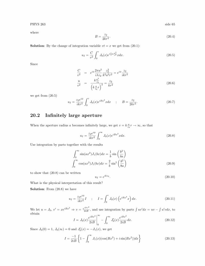
Here a is the aperture radius, and the incident field is a normally incident plane wave, as illustratedin Fig. 20.1.
20.1 Change of variable: vt → x
Show that uI can be expressed as:
uI =z2e
iφ
ikr2
∫ v
0
J0(x)eiBx2xdx (20.3)
z
u =ei ikz
sirkulær apertur
observasjons-punktr
Figure 20.1: Diffraction trough a circular aperture.
PHYS 263 side 65
whereB =
z22kr2
. (20.4)
Solution: By the change of integration variable vt = x we get from (20.1):
uI =C
v2
∫ v
0
J0(x)ei 12u
x2
v2 xdx. (20.5)
Since
C
v2= eiφ
2πa2
iλz2
z22
k2a2r2= eiφ
z2ikr2
u
v2=
k a2
z2(k az2r)2 =
z2kr2
(20.6)
we get from (20.5)
uI =z2e
iφ
ikr2
∫ v
0
J0(x)eiBx2xdx ; B =
z22kr2
. (20.7)
20.2 Infinitely large aperture
When the aperture radius a becomes infinitely large, we get v = k az2r →∞, so that
uI =z2e
iφ
ikr2
∫ ∞
0
J0(x)eiBx2xdx. (20.8)
Use integration by parts together with the results∫ ∞
0
sin(ax2)J1(bx)dx =1b
sin(b2
4a
)∫ ∞
0
cos(ax2)J1(bx)dx =2b
sin2
(b2
8a
)(20.9)
to show that (20.8) can be writtenuI = eikz2 . (20.10)
What is the physical interpretation of this result?
Solution: From (20.8) we have
uI =z2e
iφ
ikr2I ; I =
∫ v
0
J0(x)(eiBx
2x)dx. (20.11)
We let u = J0, v′ = xeiBx2 ⇒ v = eiBx2
2iB , and use integration by parts∫uv′dx = uv −
∫u′vdx, to
obtain
I = J0(x)eiBx
2
2iB
∣∣∣∣∣∞
0
−∫ ∞
0
J ′0(x)eiBx
2
2iBdx. (20.12)
Since J0(0) = 1, J0(∞) = 0 and J ′0(x) = −J1(x), we get
I =−12iB
{1−
∫ ∞
0
J1(x)(cos(Bx2) + i sin(Bx2))dx}
(20.13)
PHYS 263 side 66
which by use of the formulas in (20.9) give:
I =i
2B
{1− 2 sin2
(12· 14B
)− i sin
(1
4B
)};
14B
=kr2
2z2. (20.14)
Since 2 sin2 x2 = 1− cosx, we get
I =i
2B
(cos(
14B
)− i sin
(1
4B
))=
i
2B
(cos(−14B
)+ i sin
(−14B
))=
i
2Be−i
14B =
2i4B
e−i1
4B = 2ikr2
2z2e−i
kr22z2 =
ikr2
z2e−i
kr22z2 . (20.15)
Substitution for I from (20.15) and for φ from (20.2) in (20.11) gives
uI =z2e
ik(z2+r22z2
)
ikr2ikr2
z2e−i
kr22z2 = eikz2 . (20.16)
The physical interpretation of this result is that when the aperture is infinitely large, the incidentplane propagates along without obstruction of any kind.
PHYS 263 side 67
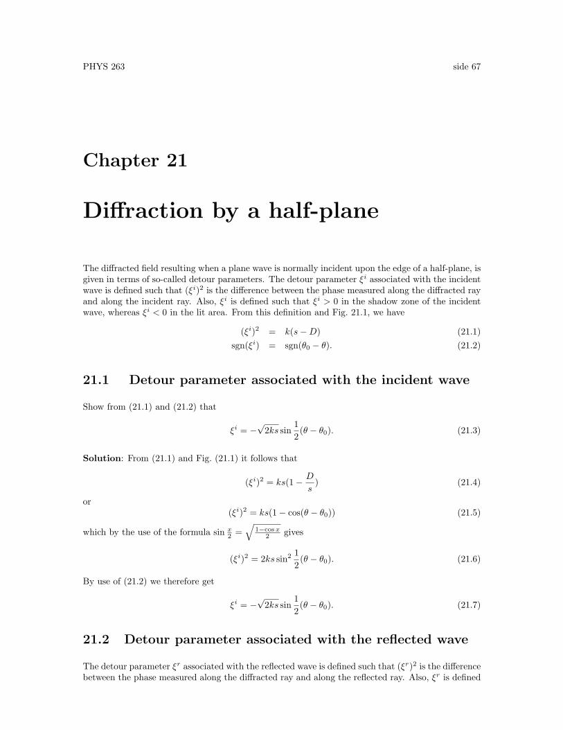
Chapter 21
Diffraction by a half-plane
The diffracted field resulting when a plane wave is normally incident upon the edge of a half-plane, isgiven in terms of so-called detour parameters. The detour parameter ξi associated with the incidentwave is defined such that (ξi)2 is the difference between the phase measured along the diffracted rayand along the incident ray. Also, ξi is defined such that ξi > 0 in the shadow zone of the incidentwave, whereas ξi < 0 in the lit area. From this definition and Fig. 21.1, we have
(ξi)2 = k(s−D) (21.1)sgn(ξi) = sgn(θ0 − θ). (21.2)
21.1 Detour parameter associated with the incident wave
Show from (21.1) and (21.2) that
ξi = −√
2ks sin12(θ − θ0). (21.3)
Solution: From (21.1) and Fig. (21.1) it follows that
(ξi)2 = ks(1− D
s) (21.4)
or(ξi)2 = ks(1− cos(θ − θ0)) (21.5)
which by the use of the formula sin x2 =
√1−cos x
2 gives
(ξi)2 = 2ks sin2 12(θ − θ0). (21.6)
By use of (21.2) we therefore get
ξi = −√
2ks sin12(θ − θ0). (21.7)
21.2 Detour parameter associated with the reflected wave
The detour parameter ξr associated with the reflected wave is defined such that (ξr)2 is the differencebetween the phase measured along the diffracted ray and along the reflected ray. Also, ξr is defined
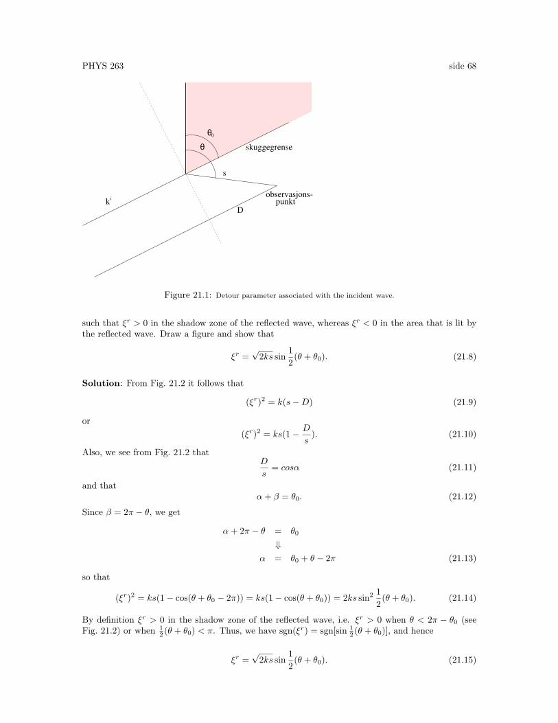
PHYS 263 side 68
s
Dk
θ
θ
i
0
skuggegrense
observasjons-punkt
Figure 21.1: Detour parameter associated with the incident wave.
such that ξr > 0 in the shadow zone of the reflected wave, whereas ξr < 0 in the area that is lit bythe reflected wave. Draw a figure and show that
ξr =√
2ks sin12(θ + θ0). (21.8)
Solution: From Fig. 21.2 it follows that
(ξr)2 = k(s−D) (21.9)
or(ξr)2 = ks(1− D
s). (21.10)
Also, we see from Fig. 21.2 thatD
s= cosα (21.11)
and thatα+ β = θ0. (21.12)
Since β = 2π − θ, we get
α+ 2π − θ = θ0
⇓α = θ0 + θ − 2π (21.13)
so that
(ξr)2 = ks(1− cos(θ + θ0 − 2π)) = ks(1− cos(θ + θ0)) = 2ks sin2 12(θ + θ0). (21.14)
By definition ξr > 0 in the shadow zone of the reflected wave, i.e. ξr > 0 when θ < 2π − θ0 (seeFig. 21.2) or when 1
2 (θ + θ0) < π. Thus, we have sgn(ξr) = sgn[sin 12 (θ + θ0)], and hence
ξr =√
2ks sin12(θ + θ0). (21.15)
PHYS 263 side 69
α
bøjgje
β
ki
skuggegrense
θ
0θ
s
D
front
punktobservasjons-
Figure 21.2: Detour parameter for the reflected wave.
PHYS 263 side 70
Chapter 22
Diffraction through a circularaperture – axial intensity
When a plane wave is normally incident upon a circular aperture, the intensity in the diffractionpattern is given by
I =(πa2
λz2
)2 ∣∣∣∣2∫ 1
0
J0(vt)ei12ut
2tdt
∣∣∣∣2 . (22.1)
Show that along the axis v = 0 the intensity becomes
I = 4 sin2(πa2/2λz2). (22.2)
Sketch the axial intensity as a function of z2 in units of a2/2λ. Give a physical interpretation ofthis axial interference pattern and explain why the minimum intensity is zero and the maximumintensity has the value of 4.
Solution: Since u = ka2/z2 = 2πa2/λz2, the given expression for the intensity distribution becomes
I =∣∣∣∣u ∫ 1
0
J0(vt)ei12ut
2tdt
∣∣∣∣2 . (22.3)
Along the axis v = 0 we have (since J0(0) = 1):
A = u
∫ 1
0
J0(vt)ei12ut
2tdt = u
∫ 1
0
ei12ut
2tdt. (22.4)
We let 12 t
2 = x, so that tdt = dx and we get:
A = u
∫ 12
0
eiuxdx = ueiux
iu
∣∣∣∣12
0
= 2ei
u2 − 12i
= 2eiu4ei
u4 − ei
−u4
2i= 2ei
u4 sin
(u4
). (22.5)
Thus, the axial intensity becomes
I = 4 sin2(u/4) = 4 sin2(πa2/2λz2). (22.6)
The axial intensity has maxima when πa2/2λz2 = (π/2)m, where m = 1, 3, 5, · · ·. Thus, we maywrite
z(m)2max =
a2
λ
1m
; m = 1, 3, 5, · · · . (22.7)
PHYS 263 side 71
The axial intensity has zeros when πa2/2λz2 = πm, where m = 1, 2, 3, · · ·. Thus, we may write
z(m)2min =
a2
λ
1m
; m = 2, 4, 6, · · · . (22.8)
When z2 is expressed in units of a2/λ, the intensity has maxima for z2 = 1, 1/3, 1/5, 1/7, · · ·, andminima when z2 = 1/2, 1/4, 1/6, 1/8, · · ·. As z2 increases beyond the value of a2/λ, the intensitydecays monotonically to zero, and as z2 decreases below the value of a2/λ, the intensity oscillatesfaster and faster between the values of zero and 4. For an aperture radius of a = 1 mm and awavelength of λ = 0.5 µm, we have a2/λ = 2 m.
The physical interpretation of this axial interference pattern is that at any observation point onthe axis the distance from the edge to the observation point is the same for all edge-diffractedrays. Hence the edge-diffracted waves interact to reinforce one another and the resulting wave dueto all edge points is of the same intensity as the incident wave. This explains why we get zerominimum intensity at axial points where the edge-diffracted wave is out of phase with the incidentwave (destructive interference). The incident plane wave is of unit amplitude, and since the totaledge-diffracted wave has the same amplitude as the incident wave, we get a total amplitude of 2, andhence an intensity of 4, at axial points where the edge-diffracted wave is in phase with the incidentwave (constructive interference).
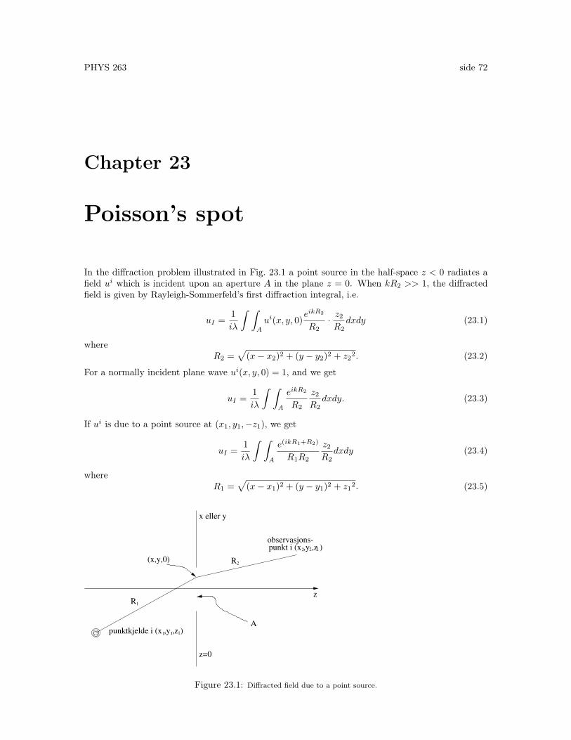
PHYS 263 side 72
Chapter 23
Poisson’s spot
In the diffraction problem illustrated in Fig. 23.1 a point source in the half-space z < 0 radiates afield ui which is incident upon an aperture A in the plane z = 0. When kR2 >> 1, the diffractedfield is given by Rayleigh-Sommerfeld’s first diffraction integral, i.e.
uI =1iλ
∫ ∫A
ui(x, y, 0)eikR2
R2· z2R2
dxdy (23.1)
whereR2 =
√(x− x2)2 + (y − y2)2 + z22. (23.2)
For a normally incident plane wave ui(x, y, 0) = 1, and we get
uI =1iλ
∫ ∫A
eikR2
R2
z2R2
dxdy. (23.3)
If ui is due to a point source at (x1, y1,−z1), we get
uI =1iλ
∫ ∫A
e(ikR1+R2)
R1R2
z2R2
dxdy (23.4)
whereR1 =
√(x− x1)2 + (y − y1)2 + z12. (23.5)
z=0
z
observasjons-
R
R
punkt i (x ,y ,z )
A
2 2
x eller y
(x,y,0)
1
2
1 1 1punktkjelde i (x ,y ,z )
2
Figure 23.1: Diffracted field due to a point source.
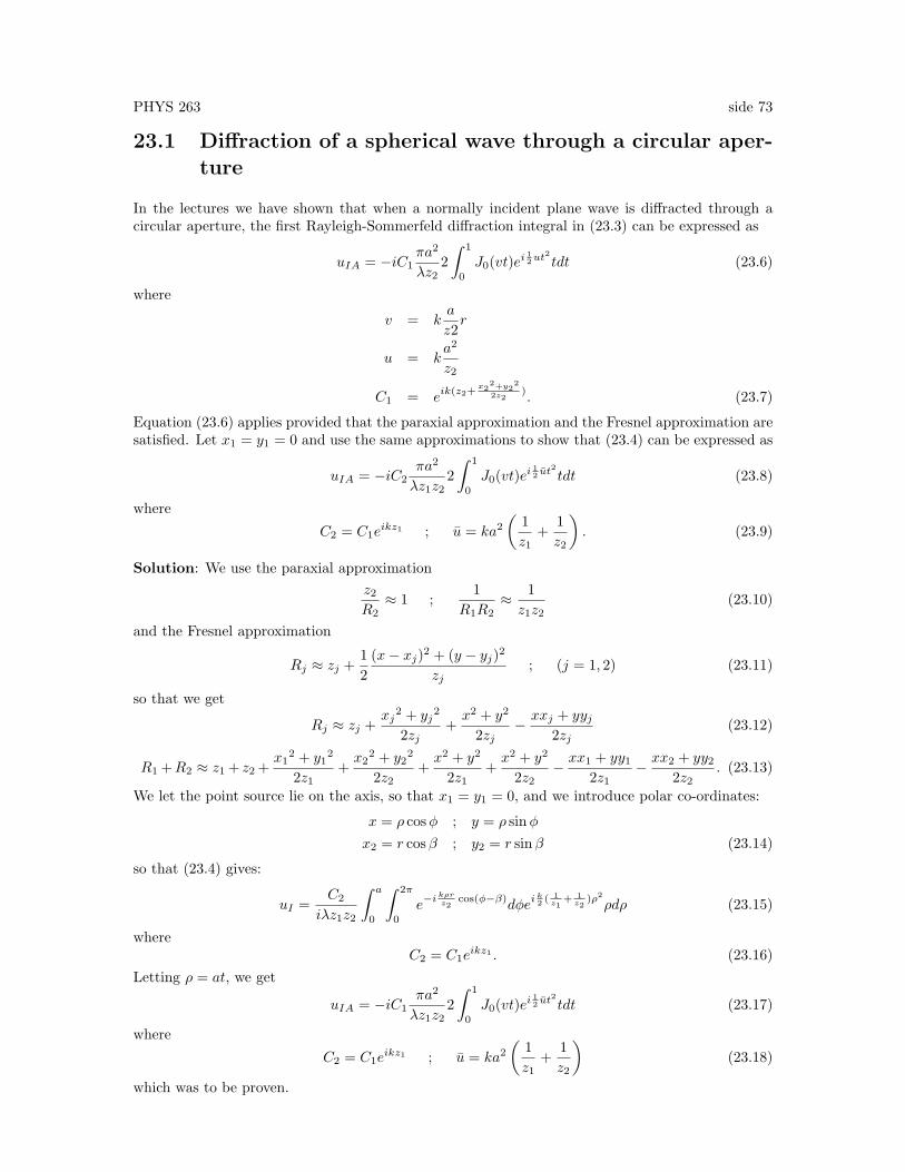
PHYS 263 side 73
23.1 Diffraction of a spherical wave through a circular aper-ture
In the lectures we have shown that when a normally incident plane wave is diffracted through acircular aperture, the first Rayleigh-Sommerfeld diffraction integral in (23.3) can be expressed as
uIA = −iC1πa2
λz22∫ 1
0
J0(vt)ei12ut
2tdt (23.6)
where
v = ka
z2r
u = ka2
z2
C1 = eik(z2+x2
2+y22
2z2). (23.7)
Equation (23.6) applies provided that the paraxial approximation and the Fresnel approximation aresatisfied. Let x1 = y1 = 0 and use the same approximations to show that (23.4) can be expressed as
uIA = −iC2πa2
λz1z22∫ 1
0
J0(vt)ei12 ut
2tdt (23.8)
where
C2 = C1eikz1 ; u = ka2
(1z1
+1z2
). (23.9)
Solution: We use the paraxial approximationz2R2
≈ 1 ;1
R1R2≈ 1z1z2
(23.10)
and the Fresnel approximation
Rj ≈ zj +12
(x− xj)2 + (y − yj)2
zj; (j = 1, 2) (23.11)
so that we get
Rj ≈ zj +xj
2 + yj2
2zj+x2 + y2
2zj− xxj + yyj
2zj(23.12)
R1 +R2 ≈ z1 + z2 +x1
2 + y12
2z1+x2
2 + y22
2z2+x2 + y2
2z1+x2 + y2
2z2− xx1 + yy1
2z1− xx2 + yy2
2z2. (23.13)
We let the point source lie on the axis, so that x1 = y1 = 0, and we introduce polar co-ordinates:
x = ρ cosφ ; y = ρ sinφx2 = r cosβ ; y2 = r sinβ (23.14)
so that (23.4) gives:
uI =C2
iλz1z2
∫ a
0
∫ 2π
0
e−ikρrz2
cos(φ−β)dφeik2 ( 1
z1+ 1
z2)ρ2ρdρ (23.15)
whereC2 = C1e
ikz1 . (23.16)Letting ρ = at, we get
uIA = −iC1πa2
λz1z22∫ 1
0
J0(vt)ei12 ut
2tdt (23.17)
where
C2 = C1eikz1 ; u = ka2
(1z1
+1z2
)(23.18)
which was to be proven.

PHYS 263 side 74
23.2 Opaque disc
Let the incident field be a normally incident plane wave, and let the circular aperture be replacedby a circular disc. Show that the diffracted field then is given by
uIS = eikz2 − uIA (23.19)
where uIA is given by (23.6).
Solution: When we replace an aperture with an opaque disc of the same shape, we can use Babinet’sprinciple, according to which uIS = ui − uIA, where uIS og uIA are the diffracted fields due to thedisc and the aperure, respectively. In the present case ui = eikz2 , and therefore we obtain (23.19).
23.3 Proof of Babinet’s principle
Let A be the aperture that is complementary to A, so that A + A covers the whole plane z = 0.Then we have
uIA = − 12π
∫ ∫A
ui∂
∂z2
(eikR2
R2
)dxdy
uIS = − 12π
∫ ∫A
ui∂
∂z2
(eikR2
R2
)dxdy
= − 12π
∫ ∫ ∞
−∞ui
∂
∂z2
(eikR2
R2
)dxdy
−(− 1
2π
∫ ∫A
ui∂
∂z2
(eikR2
R2
)dxdy
). (23.20)
The first integral gives after the last equality sign in (23.20) gives ui, because the integration is overthe entire plane (i.e. no edge diffraction) and the final integral in (23.20) gives uIA. Thus, we haveBabinet’s principle, uIS = ui − uIA.
23.4 Axial field - incident plane wave
Show that on the axis v = 0 we get from (23.19)
uIS = eik(z2+
r22z2
)(23.21)
which implies that the intensity everywhere on the axis behind an opaque circular disc is the sameas the intensity of the incident plane wave! This bright spot is Poisson′s spot, named after Poissonwho first predicted it on the basis of Fresnel’s wave theory. Poisson used this bright spot as a proofagainst the wave theory. But when Arago soon afterwards carried out the experiment, he observedthe bright spot on the axis.
Solution: On the axis x2 = y2 = 0 we have [see (23.6)]:
−uIA = +ieikz2uJ ; u =2πλ
a2
z2
J =∫ 1
0
ei12ut
2dt ;
12t2 = x⇒ tdt = dx (23.22)

PHYS 263 side 75
⇒ J =∫ 1
2
0
eiuxdx =eiux
iu
∣∣∣∣12
0
=ei
u2 − 1iu
⇒ −uIA = eikz2(eiu2 − 1). (23.23)
Thus, we have from (23.19)
uIS = eikz2 − uIA = eikz2+iu2 = eik(z2+
a22z2
). (23.24)
The intensity becomes|uIS |2 = |uI |2. (23.25)
23.5 Axial field - incident spherical wave
Repeat the derivations in Exercises 23.2 and 23.4 for an incident diverging spherical wave, sothat (23.8) applies. Consider the special case in which z1 = z2 and try to simplify the result asmuch as possible.
Solution: According to Babinet’s principle we have uIS = U i − uIA. At the point x2 = y2 = 0 onthe axis ui is given by:
ui =eik(z1+z2)
z1 + z2(23.26)
and from (23.8) with x2 = y2 = v = 0 we get
−uIA = ieik(z1+z2) · k a2
z1z2
eiu2 − 1iu
. (23.27)
Since u = ka2( 1z1
+ 1z2
) [see (23.9)], we get
−uIA = −ui +eik(z1+z2)+iu/2
z1 + z2(23.28)
so that
uIS = ui − uIA =exp
{ik (z1 + z2)
(1 + a2
2z1z2))}
z1 + z2. (23.29)
The on-axis intensity becomes
|uIS |2 =(
1z1 + z2
)2
= |ui|2. (23.30)
Thus, on the axis behind a circular opaque disc the intensity is the same as if the disc were removed!If we let z1 = z2, we get
|uIS |2 =14
(1z1
)2
(23.31)
which implies that the intensity at this observation point on the axis is one quarter of the incidentintensity at the center of the disc. When z1 >> z2,we get from (23.30)
|uIS |2 =(
1z1
)2(
11 + z2
z1
)2
≈(
1z1
)2
(23.32)
where(
1z1
)2
is the intensity of the incident wave at the center of the disc, in accordance with theresult from Exercise 23.4.
PHYS 263 side 76
Chapter 24
Fraunhofer diffraction at obliqueincidence and interference betweenthe fields diffracted through twoapertures
In the lectures we have shown that the diffracted field in the Fraunhofer zone is given by
uI =C1
iλz2
∫ ∫ ∞
∞ui(x, y, 0)t(x, y)e−i(k
0xx+k
0yy)dxdy (24.1)
where
C1 = eik
(z2+
x22+y2
2
2z2
); k0
x =kx2
z2; k0
y =ky2z2
(24.2)
and where ui is the incident field and t(x, y) is the transmission function of the aperture. Let usassume that t(x, y) has the value 1 when (x, y) lies inside the aperture A and the value zero when(x, y) lies outside A.
24.1 Fourier representation at oblique incidence
Show that for an obliquely incident plane wave with wave vector
ki = kxiex + ky
iey + kziez (24.3)
the diffracted field becomesuI =
C1
iλz2
∫ ∫A
e−i(Kxx+Kyy)dxdy (24.4)
whereKx = k0
x − kix ; Ky = k0y − kiy. (24.5)
Solution: The obliquely incident plane is given by
ui = eik·r = ei(kxix+ky
iy+kziz) (24.6)
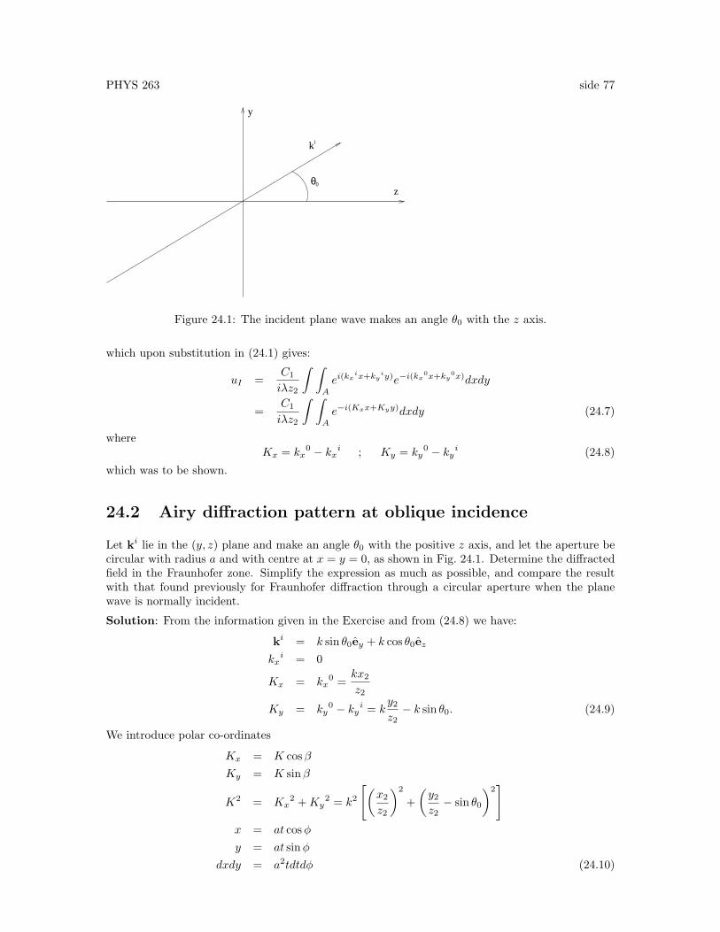
PHYS 263 side 77
y
zθ
k
0
i
Figure 24.1: The incident plane wave makes an angle θ0 with the z axis.
which upon substitution in (24.1) gives:
uI =C1
iλz2
∫ ∫A
ei(kxix+ky
iy)e−i(kx0x+ky
0x)dxdy
=C1
iλz2
∫ ∫A
e−i(Kxx+Kyy)dxdy (24.7)
whereKx = kx
0 − kxi ; Ky = ky
0 − kyi (24.8)
which was to be shown.
24.2 Airy diffraction pattern at oblique incidence
Let ki lie in the (y, z) plane and make an angle θ0 with the positive z axis, and let the aperture becircular with radius a and with centre at x = y = 0, as shown in Fig. 24.1. Determine the diffractedfield in the Fraunhofer zone. Simplify the expression as much as possible, and compare the resultwith that found previously for Fraunhofer diffraction through a circular aperture when the planewave is normally incident.
Solution: From the information given in the Exercise and from (24.8) we have:
ki = k sin θ0ey + k cos θ0ezkxi = 0
Kx = kx0 =
kx2
z2
Ky = ky0 − ky
i = ky2z2− k sin θ0. (24.9)
We introduce polar co-ordinates
Kx = K cosβKy = K sinβ
K2 = Kx2 +Ky
2 = k2
[(x2
z2
)2
+(y2z2− sin θ0
)2]
x = at cosφy = at sinφ
dxdy = a2tdtdφ (24.10)
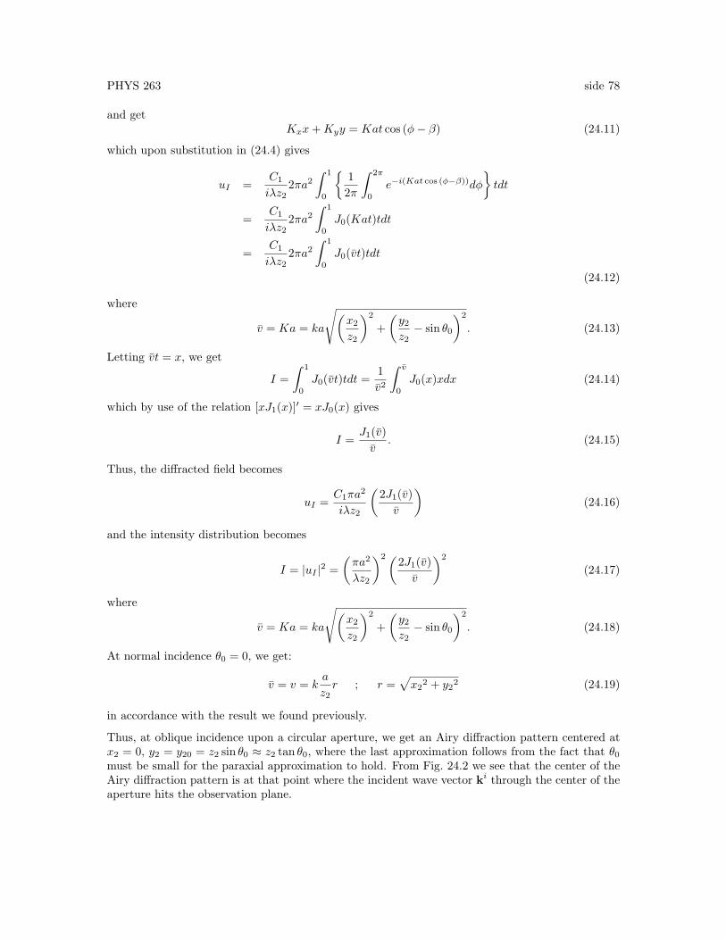
PHYS 263 side 78
and getKxx+Kyy = Kat cos (φ− β) (24.11)
which upon substitution in (24.4) gives
uI =C1
iλz22πa2
∫ 1
0
{12π
∫ 2π
0
e−i(Kat cos (φ−β))dφ
}tdt
=C1
iλz22πa2
∫ 1
0
J0(Kat)tdt
=C1
iλz22πa2
∫ 1
0
J0(vt)tdt
(24.12)
where
v = Ka = ka
√(x2
z2
)2
+(y2z2− sin θ0
)2
. (24.13)
Letting vt = x, we get
I =∫ 1
0
J0(vt)tdt =1v2
∫ v
0
J0(x)xdx (24.14)
which by use of the relation [xJ1(x)]′ = xJ0(x) gives
I =J1(v)v
. (24.15)
Thus, the diffracted field becomes
uI =C1πa
2
iλz2
(2J1(v)v
)(24.16)
and the intensity distribution becomes
I = |uI |2 =(πa2
λz2
)2(2J1(v)v
)2
(24.17)
where
v = Ka = ka
√(x2
z2
)2
+(y2z2− sin θ0
)2
. (24.18)
At normal incidence θ0 = 0, we get:
v = v = ka
z2r ; r =
√x2
2 + y22 (24.19)
in accordance with the result we found previously.
Thus, at oblique incidence upon a circular aperture, we get an Airy diffraction pattern centered atx2 = 0, y2 = y20 = z2 sin θ0 ≈ z2 tan θ0, where the last approximation follows from the fact that θ0must be small for the paraxial approximation to hold. From Fig. 24.2 we see that the center of theAiry diffraction pattern is at that point where the incident wave vector ki through the center of theaperture hits the observation plane.

PHYS 263 side 79
y
θ
k
0
i
sirkulær
apertur
z
Airy mønsteretSentrum i
z
y20
2
Figure 24.2: The center of the Airy diffraction pattern is at the point where ki through the centerof the aperture hits the observation plane.
x
y y’=y-
A
A’
s
η
β
x’=x- ξ1
1
0
Figure 24.3: The aperture A′ is displaced relative to A
24.3 Aperture displacement
Show that if we displace the aperture A in the plane z = 0 in (24.4) a distance s in a direction thatmakes an angle β0 with the positive x axis, then the diffracted field u′I due to the new aperture A′
is given byu′I = uIe
−i(Kxξ1+Kyη1) (24.20)
whereξ1 = s cosβ0 ; η1 = s sinβ0 (24.21)
is the origin in a displaced co-ordinate system (x′, y′) that is related to A′ in the same way as theoriginal co-ordinate system (x, y) is related to A
Solution: A og A′ are identical apertures, which are displaced relative to one another, as illustratedin Fig. 24.3. The diffracted field due to A′ is given by:
u′I =C1
iλz2
∫ ∫A′e−i(Kxx+Kyy)dxdy. (24.22)
Letting x′ = x− ξ1 og y′ = y − η1, we get
u′I =C1
iλz2e−i(Kxξ1+Kyη1)
∫ ∫A′e−i(Kxx
′+Kyy′)dx′dy′
PHYS 263 side 80
= e−i(Kxξ1+Kyη1)C1
iλz2
∫ ∫A
e−i(Kxx+Kyy)dxdy (24.23)
oru′I = uIe
−i(Kxξ1+Kyη1) (24.24)
which was to be shown.
24.4 Interference
Use the result from Exercise 24.3 to show that the diffracted intensity due to both A and A′ is givenby
I = 4I0 cos2(
12δ
)(24.25)
where I0 is the intensity due to A or A′ alone, and where
δ = Kxξ1 +Kyη1. (24.26)
Solution: The diffracted field uIt due to A and A′ becomes
uIt = uI + u′I = uI(1 + e−iδ) (24.27)
where δ = Kxξ1 +Kyη1 and where uI is the diffracted field due to A alone. The intensity becomes:
It = |uIt|2 = |uI |2(2 + 2 cos δ) = 2I0(1 + cos δ) (24.28)
orIt = 4I0 cos2
δ
2(24.29)
whereI0 = |uI |2. (24.30)
24.5 Example
Sketch the diffraction pattern given by (24.25) for the case in which we have two circular apertureswith radius a = 0.1 mm and normal incidence. Let the other parameters be β0 = 0, s = 1 mm, λ =0.5 µm, and z2 = 10 m. How large is the diameter of the Airy disc, and how many dark interferencefringes are there inside the Airy disc?
Solution: For two circular apertures I0 is the Airy diffraction pattern and cos2 12δ gives straight
interference fringes that are oriented normally to the line connecting the two apertures. This isillustrated in Fig. 24.4. The diameter of the Airy disc is given by D = 2r0, where v0 = k a
z2r0 = 3.83.
This gives
D = 2.44 ·( z2
2a
)λ = 2.44 · 10
2 · 0.1 · 10−3· 0.5 · 10−6 m = 6.1 cm. (24.31)
The factor cos2 12δ gives a dark interference fringe when
12δ = (nπ +
π
2) ; (n = ±1, 2, 3, ...)
⇓δ = n2π + π. (24.32)
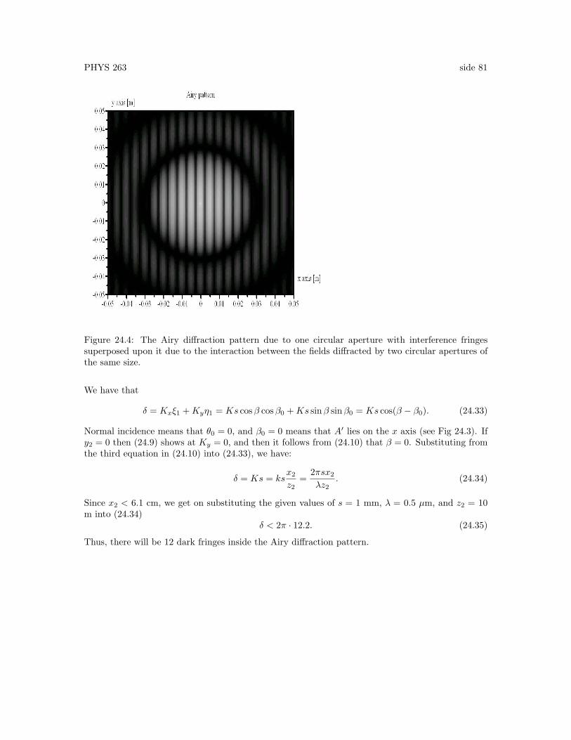
PHYS 263 side 81
Figure 24.4: The Airy diffraction pattern due to one circular aperture with interference fringessuperposed upon it due to the interaction between the fields diffracted by two circular apertures ofthe same size.
We have that
δ = Kxξ1 +Kyη1 = Ks cosβ cosβ0 +Ks sinβ sinβ0 = Ks cos(β − β0). (24.33)
Normal incidence means that θ0 = 0, and β0 = 0 means that A′ lies on the x axis (see Fig 24.3). Ify2 = 0 then (24.9) shows at Ky = 0, and then it follows from (24.10) that β = 0. Substituting fromthe third equation in (24.10) into (24.33), we have:
δ = Ks = ksx2
z2=
2πsx2
λz2. (24.34)
Since x2 < 6.1 cm, we get on substituting the given values of s = 1 mm, λ = 0.5 µm, and z2 = 10m into (24.34)
δ < 2π · 12.2. (24.35)
Thus, there will be 12 dark fringes inside the Airy diffraction pattern.