Embed Size (px)
Citation preview

PHYS 405 - Fundamentals of Quantum Theory I
Term: Fall 2013Meetings: Monday & Wednesday 11:25-12:40Location: 220 Stuart Building
Instructor: Carlo SegreOffice: 166A Life SciencesPhone: 312.567.3498email: [email protected]
Book: Introduction to Quantum Mechanics, 2nd ed.,D. Griffiths (Pearson, 2005)
Web Site: http://phys.iit.edu/∼segre/phys405/13F
C. Segre (IIT) PHYS 405 - Fall 2013 August 19, 2013 1 / 23

Course Objectives
1 Understand the interpretation of the Schrodinger equation and thewave function.
2 Understand the solution of the time-independent Schrodingerequation for one-dimensional potentials.
3 Understand quantum formalism including operators and the Diracnotation.
4 Understand the solution of three-dimensional potentials.
5 Understand how systems of identical particles are solved.
6 Be able to solve quantum mechanics problems in one and threedimensions and with identical particles.
C. Segre (IIT) PHYS 405 - Fall 2013 August 19, 2013 2 / 23

Course Grading
10% – Homework assignments
Weekly or bi-weeklyDue at beginning of classMay be turned in via Blackboard
5% – Class participation (work in progress)
50% – Two mid-term exams
35% – Final examination (08:00 Dec. 03)
Grading scaleA – 88% to 100%B – 75% to 88%C – 62% to 75%D – 50% to 62%E – 0% to 50%
C. Segre (IIT) PHYS 405 - Fall 2013 August 19, 2013 3 / 23

Course Grading
10% – Homework assignmentsWeekly or bi-weekly
Due at beginning of classMay be turned in via Blackboard
5% – Class participation (work in progress)
50% – Two mid-term exams
35% – Final examination (08:00 Dec. 03)
Grading scaleA – 88% to 100%B – 75% to 88%C – 62% to 75%D – 50% to 62%E – 0% to 50%
C. Segre (IIT) PHYS 405 - Fall 2013 August 19, 2013 3 / 23

Course Grading
10% – Homework assignmentsWeekly or bi-weeklyDue at beginning of class
May be turned in via Blackboard
5% – Class participation (work in progress)
50% – Two mid-term exams
35% – Final examination (08:00 Dec. 03)
Grading scaleA – 88% to 100%B – 75% to 88%C – 62% to 75%D – 50% to 62%E – 0% to 50%
C. Segre (IIT) PHYS 405 - Fall 2013 August 19, 2013 3 / 23

Course Grading
10% – Homework assignmentsWeekly or bi-weeklyDue at beginning of classMay be turned in via Blackboard
5% – Class participation (work in progress)
50% – Two mid-term exams
35% – Final examination (08:00 Dec. 03)
Grading scaleA – 88% to 100%B – 75% to 88%C – 62% to 75%D – 50% to 62%E – 0% to 50%
C. Segre (IIT) PHYS 405 - Fall 2013 August 19, 2013 3 / 23

Topics to be Covered (Chapter titles)
1 The wave function
2 Time-independent Schrodinger equation
3 Quantum formalism
4 Three dimensional quantum mechanics
5 Identical particles
6 Other topics as appropriate
C. Segre (IIT) PHYS 405 - Fall 2013 August 19, 2013 4 / 23

Topics to be Covered (Chapter titles)
1 The wave function
2 Time-independent Schrodinger equation
3 Quantum formalism
4 Three dimensional quantum mechanics
5 Identical particles
6 Other topics as appropriate
C. Segre (IIT) PHYS 405 - Fall 2013 August 19, 2013 4 / 23

Topics to be Covered (Chapter titles)
1 The wave function
2 Time-independent Schrodinger equation
3 Quantum formalism
4 Three dimensional quantum mechanics
5 Identical particles
6 Other topics as appropriate
C. Segre (IIT) PHYS 405 - Fall 2013 August 19, 2013 4 / 23

Topics to be Covered (Chapter titles)
1 The wave function
2 Time-independent Schrodinger equation
3 Quantum formalism
4 Three dimensional quantum mechanics
5 Identical particles
6 Other topics as appropriate
C. Segre (IIT) PHYS 405 - Fall 2013 August 19, 2013 4 / 23

Topics to be Covered (Chapter titles)
1 The wave function
2 Time-independent Schrodinger equation
3 Quantum formalism
4 Three dimensional quantum mechanics
5 Identical particles
6 Other topics as appropriate
C. Segre (IIT) PHYS 405 - Fall 2013 August 19, 2013 4 / 23

Topics to be Covered (Chapter titles)
1 The wave function
2 Time-independent Schrodinger equation
3 Quantum formalism
4 Three dimensional quantum mechanics
5 Identical particles
6 Other topics as appropriate
C. Segre (IIT) PHYS 405 - Fall 2013 August 19, 2013 4 / 23

Course Schedule
Up-to-date schedule athttp://phys.iit.edu/∼segre/phys405/13F/schedule.html
27 class sessions
2 mid-term exams
∼250 pages to cover
∼20 pages/week
Focus on “mechanics” but will bring in some philosophy as well.
C. Segre (IIT) PHYS 405 - Fall 2013 August 19, 2013 5 / 23

Course Schedule
Up-to-date schedule athttp://phys.iit.edu/∼segre/phys405/13F/schedule.html
27 class sessions
2 mid-term exams
∼250 pages to cover
∼20 pages/week
Focus on “mechanics” but will bring in some philosophy as well.
C. Segre (IIT) PHYS 405 - Fall 2013 August 19, 2013 5 / 23

Course Schedule
Up-to-date schedule athttp://phys.iit.edu/∼segre/phys405/13F/schedule.html
27 class sessions
2 mid-term exams
∼250 pages to cover
∼20 pages/week
Focus on “mechanics” but will bring in some philosophy as well.
C. Segre (IIT) PHYS 405 - Fall 2013 August 19, 2013 5 / 23

Course Schedule
Up-to-date schedule athttp://phys.iit.edu/∼segre/phys405/13F/schedule.html
27 class sessions
2 mid-term exams
∼250 pages to cover
∼20 pages/week
Focus on “mechanics” but will bring in some philosophy as well.
C. Segre (IIT) PHYS 405 - Fall 2013 August 19, 2013 5 / 23

Course Schedule
Up-to-date schedule athttp://phys.iit.edu/∼segre/phys405/13F/schedule.html
27 class sessions
2 mid-term exams
∼250 pages to cover
∼20 pages/week
Focus on “mechanics” but will bring in some philosophy as well.
C. Segre (IIT) PHYS 405 - Fall 2013 August 19, 2013 5 / 23

Course Schedule
Up-to-date schedule athttp://phys.iit.edu/∼segre/phys405/13F/schedule.html
27 class sessions
2 mid-term exams
∼250 pages to cover
∼20 pages/week
Focus on “mechanics” but will bring in some philosophy as well.
C. Segre (IIT) PHYS 405 - Fall 2013 August 19, 2013 5 / 23

Tips for success
1 Do the reading assignments before lecture, you willunderstand them better.
2 Attend class or really view the lectures completely, thereare things discussed which are not on the slides or thebook.
3 Ask questions in class, it’s likely that others have thesame ones.
4 Go through the derivations yourself, kill some trees!
5 Do the homework the “right” way, only use the solutionsmanual as a last resort.
6 Come to office hours with questions, I’ll be less lonelyand it will help you too!
C. Segre (IIT) PHYS 405 - Fall 2013 August 19, 2013 6 / 23

Today’s Outline - August 19, 2013
• Black-body radiation
• Photoelectric effect
• Compton scattering
• Davisson-Germer experiment
• The 1-D Schrodinger equation
Reading Assignment: Chapter 1.1–1.6
C. Segre (IIT) PHYS 405 - Fall 2013 August 19, 2013 7 / 23

Today’s Outline - August 19, 2013
• Black-body radiation
• Photoelectric effect
• Compton scattering
• Davisson-Germer experiment
• The 1-D Schrodinger equation
Reading Assignment: Chapter 1.1–1.6
C. Segre (IIT) PHYS 405 - Fall 2013 August 19, 2013 7 / 23

Today’s Outline - August 19, 2013
• Black-body radiation
• Photoelectric effect
• Compton scattering
• Davisson-Germer experiment
• The 1-D Schrodinger equation
Reading Assignment: Chapter 1.1–1.6
C. Segre (IIT) PHYS 405 - Fall 2013 August 19, 2013 7 / 23

Today’s Outline - August 19, 2013
• Black-body radiation
• Photoelectric effect
• Compton scattering
• Davisson-Germer experiment
• The 1-D Schrodinger equation
Reading Assignment: Chapter 1.1–1.6
C. Segre (IIT) PHYS 405 - Fall 2013 August 19, 2013 7 / 23

Today’s Outline - August 19, 2013
• Black-body radiation
• Photoelectric effect
• Compton scattering
• Davisson-Germer experiment
• The 1-D Schrodinger equation
Reading Assignment: Chapter 1.1–1.6
C. Segre (IIT) PHYS 405 - Fall 2013 August 19, 2013 7 / 23

Today’s Outline - August 19, 2013
• Black-body radiation
• Photoelectric effect
• Compton scattering
• Davisson-Germer experiment
• The 1-D Schrodinger equation
Reading Assignment: Chapter 1.1–1.6
C. Segre (IIT) PHYS 405 - Fall 2013 August 19, 2013 7 / 23

Today’s Outline - August 19, 2013
• Black-body radiation
• Photoelectric effect
• Compton scattering
• Davisson-Germer experiment
• The 1-D Schrodinger equation
Reading Assignment: Chapter 1.1–1.6
C. Segre (IIT) PHYS 405 - Fall 2013 August 19, 2013 7 / 23

Black Body Radiation
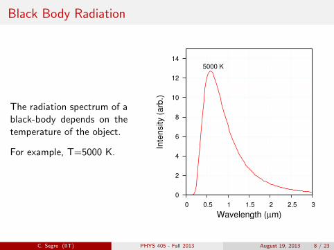
The radiation spectrum of ablack-body depends on thetemperature of the object.
For example, T=5000 K.
0
2
4
6
8
10
12
14
0 0.5 1 1.5 2 2.5 3
Inte
nsity (
arb
.)
Wavelength (µm)
5000 K
C. Segre (IIT) PHYS 405 - Fall 2013 August 19, 2013 8 / 23
Black Body Radiation
The radiation spectrum of ablack-body depends on thetemperature of the object.
For example, T=5000 K.
0
2
4
6
8
10
12
14
0 0.5 1 1.5 2 2.5 3
Inte
nsity (
arb
.)
Wavelength (µm)
5000 K
C. Segre (IIT) PHYS 405 - Fall 2013 August 19, 2013 8 / 23

Black Body Radiation
The maximum wavelengthλm is seen to scale inverselywith temperature such that
λmT = 2.898× 10⁻³m · K3
0
2
4
6
8
10
12
14
0 0.5 1 1.5 2 2.5 3
Inte
nsity (
arb
.)
Wavelength (µm)
5000 K
C. Segre (IIT) PHYS 405 - Fall 2013 August 19, 2013 8 / 23

Black Body Radiation
The maximum wavelengthλm is seen to scale inverselywith temperature such that
λmT = 2.898× 10⁻³m · K3
0
2
4
6
8
10
12
14
0 0.5 1 1.5 2 2.5 3
Inte
nsity (
arb
.)
Wavelength (µm)
5000 K
4000 K
3000 K
C. Segre (IIT) PHYS 405 - Fall 2013 August 19, 2013 8 / 23

Black Body Radiation
The maximum wavelengthλm is seen to scale inverselywith temperature such that
λmT = 2.898× 10⁻³m · K3
0
2
4
6
8
10
12
14
0 0.5 1 1.5 2 2.5 3
Inte
nsity (
arb
.)
Wavelength (µm)
5000 K
4000 K
3000 K
C. Segre (IIT) PHYS 405 - Fall 2013 August 19, 2013 8 / 23

Black Body Radiation
This proves to be a universalcurve.
However, the classical the-oretical model (Rayleigh–Jeans), is unable to describethe low wavelength cutoffobserved.∫ ∞0
u(λ)dλ ∝∫ ∞0
λ−4dλ→∞
0
2
4
6
8
10
12
14
0 0.5 1 1.5 2 2.5 3
Inte
nsity (
arb
.)
Wavelength (µm)
5000 K
4000 K
3000 K
C. Segre (IIT) PHYS 405 - Fall 2013 August 19, 2013 8 / 23

Black Body Radiation
This proves to be a universalcurve.
However, the classical the-oretical model (Rayleigh–Jeans), is unable to describethe low wavelength cutoffobserved.
∫ ∞0
u(λ)dλ ∝∫ ∞0
λ−4dλ→∞
0
2
4
6
8
10
12
14
0 0.5 1 1.5 2 2.5 3
Inte
nsity (
arb
.)
Wavelength (µm)
5000 K
4000 K
3000 K
C. Segre (IIT) PHYS 405 - Fall 2013 August 19, 2013 8 / 23

Black Body Radiation
This proves to be a universalcurve.
However, the classical the-oretical model (Rayleigh–Jeans), is unable to describethe low wavelength cutoffobserved.∫ ∞0
u(λ)dλ ∝∫ ∞0
λ−4dλ→∞
0
2
4
6
8
10
12
14
0 0.5 1 1.5 2 2.5 3
Inte
nsity (
arb
.)
Wavelength (µm)
5000 K
4000 K
3000 K
Rayleigh-Jeans(5000 K)
C. Segre (IIT) PHYS 405 - Fall 2013 August 19, 2013 8 / 23

Planck’s Solution
By assuming that the modesof oscillation in the black-body cavity were quantized.
The resulting function forthe energy distribution is
which cuts off properly asλ→ 0.
Em = mhν, m = 0, 1, 2, 3, · · ·
u(λ) ∝ λ−5
ehc/λkT − 1
limλ→0
u(λ) =e−hc/λkT
λ5
C. Segre (IIT) PHYS 405 - Fall 2013 August 19, 2013 9 / 23

Photoelectric Effect
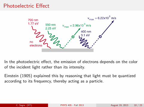
In the photoelectric effect, the emission of electrons depends on the colorof the incident light rather than its intensity.
Einstein (1905) explained this by reasoning that light must be quantizedaccording to its frequency, thereby acting as a particle.
1
2mv2max = hν − φ
C. Segre (IIT) PHYS 405 - Fall 2013 August 19, 2013 10 / 23
Photoelectric Effect
In the photoelectric effect, the emission of electrons depends on the colorof the incident light rather than its intensity.
Einstein (1905) explained this by reasoning that light must be quantizedaccording to its frequency, thereby acting as a particle.
1
2mv2max = hν − φ
C. Segre (IIT) PHYS 405 - Fall 2013 August 19, 2013 10 / 23

Compton Scattering Experiment
In 1923, Arthur Compton mea-sured the scattering of x-raysfrom a carbon foil.
He observed x-rays at lower en-ergies than the incident energyand that the energy dependedon the observation angle.
This could be explained bytreating the x-rays as particlescolliding with the electrons inthe carbon atoms of the foil.
C. Segre (IIT) PHYS 405 - Fall 2013 August 19, 2013 11 / 23

Compton Scattering Phenomenon
A photon-electron collision
ϕ
θ
λ
v
λ’
p = ~k = 2π~/λp′ = ~k′ = 2π~/λ′
|k| 6=∣∣k′∣∣
Treat the electron relativistically and conserve energy and momentum
mc2 +hc
λ=
hc
λ′+ γmc2 (energy)
h
λ=
h
λ′cosφ+ γmv cos θ (x-axis)
0 =h
λ′sinφ+ γmv sin θ (y-axis)
C. Segre (IIT) PHYS 405 - Fall 2013 August 19, 2013 12 / 23

Compton Scattering Phenomenon
A photon-electron collision
ϕ
θ
λ
v
λ’
p = ~k = 2π~/λ
p′ = ~k′ = 2π~/λ′
|k| 6=∣∣k′∣∣
Treat the electron relativistically and conserve energy and momentum
mc2 +hc
λ=
hc
λ′+ γmc2 (energy)
h
λ=
h
λ′cosφ+ γmv cos θ (x-axis)
0 =h
λ′sinφ+ γmv sin θ (y-axis)
C. Segre (IIT) PHYS 405 - Fall 2013 August 19, 2013 12 / 23

Compton Scattering Phenomenon
A photon-electron collision
ϕ
θ
λ
v
λ’
p = ~k = 2π~/λp′ = ~k′ = 2π~/λ′
|k| 6=∣∣k′∣∣
Treat the electron relativistically and conserve energy and momentum
mc2 +hc
λ=
hc
λ′+ γmc2 (energy)
h
λ=
h
λ′cosφ+ γmv cos θ (x-axis)
0 =h
λ′sinφ+ γmv sin θ (y-axis)
C. Segre (IIT) PHYS 405 - Fall 2013 August 19, 2013 12 / 23

Compton Scattering Phenomenon
A photon-electron collision
ϕ
θ
λ
v
λ’
p = ~k = 2π~/λp′ = ~k′ = 2π~/λ′
|k| 6=∣∣k′∣∣
Treat the electron relativistically and conserve energy and momentum
mc2 +hc
λ=
hc
λ′+ γmc2 (energy)
h
λ=
h
λ′cosφ+ γmv cos θ (x-axis)
0 =h
λ′sinφ+ γmv sin θ (y-axis)
C. Segre (IIT) PHYS 405 - Fall 2013 August 19, 2013 12 / 23

Compton Scattering Derivation
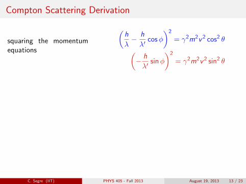
squaring the momentumequations
(h
λ− h
λ′cosφ
)2
= γ2m2v2 cos2 θ(− h
λ′sinφ
)2
= γ2m2v2 sin2 θ
now add them together, substitute sin2 θ + cos2 θ = 1, expand the squares,and sin2 φ+ cos2 φ = 1, then rearrange and substitute v = βc
γ2m2v2(sin2 θ + cos2 θ
)=
(h
λ− h
λ′cosφ
)2
+
(− h
λ′sinφ
)2
γ2m2v2 =h2
λ2− 2h2
λλ′cosφ+
h2
λ′2sin2 φ+
h2
λ′2cos2 φ
m2c2β2
1− β2=
m2v2
1− β2=
h2
λ2− 2h2
λλ′cosφ+
h2
λ′2
C. Segre (IIT) PHYS 405 - Fall 2013 August 19, 2013 13 / 23

Compton Scattering Derivation
squaring the momentumequations
(h
λ− h
λ′cosφ
)2
= γ2m2v2 cos2 θ
(− h
λ′sinφ
)2
= γ2m2v2 sin2 θ
now add them together, substitute sin2 θ + cos2 θ = 1, expand the squares,and sin2 φ+ cos2 φ = 1, then rearrange and substitute v = βc
γ2m2v2(sin2 θ + cos2 θ
)=
(h
λ− h
λ′cosφ
)2
+
(− h
λ′sinφ
)2
γ2m2v2 =h2
λ2− 2h2
λλ′cosφ+
h2
λ′2sin2 φ+
h2
λ′2cos2 φ
m2c2β2
1− β2=
m2v2
1− β2=
h2
λ2− 2h2
λλ′cosφ+
h2
λ′2
C. Segre (IIT) PHYS 405 - Fall 2013 August 19, 2013 13 / 23
Compton Scattering Derivation
squaring the momentumequations
(h
λ− h
λ′cosφ
)2
= γ2m2v2 cos2 θ(− h
λ′sinφ
)2
= γ2m2v2 sin2 θ
now add them together, substitute sin2 θ + cos2 θ = 1, expand the squares,and sin2 φ+ cos2 φ = 1, then rearrange and substitute v = βc
γ2m2v2(sin2 θ + cos2 θ
)=
(h
λ− h
λ′cosφ
)2
+
(− h
λ′sinφ
)2
γ2m2v2 =h2
λ2− 2h2
λλ′cosφ+
h2
λ′2sin2 φ+
h2
λ′2cos2 φ
m2c2β2
1− β2=
m2v2
1− β2=
h2
λ2− 2h2
λλ′cosφ+
h2
λ′2
C. Segre (IIT) PHYS 405 - Fall 2013 August 19, 2013 13 / 23

Compton Scattering Derivation
squaring the momentumequations
(h
λ− h
λ′cosφ
)2
= γ2m2v2 cos2 θ(− h
λ′sinφ
)2
= γ2m2v2 sin2 θ
now add them together,
substitute sin2 θ + cos2 θ = 1, expand the squares,and sin2 φ+ cos2 φ = 1, then rearrange and substitute v = βc
γ2m2v2(sin2 θ + cos2 θ
)=
(h
λ− h
λ′cosφ
)2
+
(− h
λ′sinφ
)2
γ2m2v2 =h2
λ2− 2h2
λλ′cosφ+
h2
λ′2sin2 φ+
h2
λ′2cos2 φ
m2c2β2
1− β2=
m2v2
1− β2=
h2
λ2− 2h2
λλ′cosφ+
h2
λ′2
C. Segre (IIT) PHYS 405 - Fall 2013 August 19, 2013 13 / 23

Compton Scattering Derivation
squaring the momentumequations
(h
λ− h
λ′cosφ
)2
= γ2m2v2 cos2 θ(− h
λ′sinφ
)2
= γ2m2v2 sin2 θ
now add them together, substitute sin2 θ + cos2 θ = 1, expand the squares,
and sin2 φ+ cos2 φ = 1, then rearrange and substitute v = βc
γ2m2v2(sin2 θ + cos2 θ
)=
(h
λ− h
λ′cosφ
)2
+
(− h
λ′sinφ
)2
γ2m2v2 =h2
λ2− 2h2
λλ′cosφ+
h2
λ′2sin2 φ+
h2
λ′2cos2 φ
m2c2β2
1− β2=
m2v2
1− β2=
h2
λ2− 2h2
λλ′cosφ+
h2
λ′2
C. Segre (IIT) PHYS 405 - Fall 2013 August 19, 2013 13 / 23

Compton Scattering Derivation
squaring the momentumequations
(h
λ− h
λ′cosφ
)2
= γ2m2v2 cos2 θ(− h
λ′sinφ
)2
= γ2m2v2 sin2 θ
now add them together, substitute sin2 θ + cos2 θ = 1, expand the squares,and sin2 φ+ cos2 φ = 1, then rearrange
and substitute v = βc
γ2m2v2(sin2 θ + cos2 θ
)=
(h
λ− h
λ′cosφ
)2
+
(− h
λ′sinφ
)2
γ2m2v2 =h2
λ2− 2h2
λλ′cosφ+
h2
λ′2sin2 φ+
h2
λ′2cos2 φ
m2c2β2
1− β2=
m2v2
1− β2=
h2
λ2− 2h2
λλ′cosφ+
h2
λ′2
C. Segre (IIT) PHYS 405 - Fall 2013 August 19, 2013 13 / 23

Compton Scattering Derivation
squaring the momentumequations
(h
λ− h
λ′cosφ
)2
= γ2m2v2 cos2 θ(− h
λ′sinφ
)2
= γ2m2v2 sin2 θ
now add them together, substitute sin2 θ + cos2 θ = 1, expand the squares,and sin2 φ+ cos2 φ = 1, then rearrange and substitute v = βc
γ2m2v2(sin2 θ + cos2 θ
)=
(h
λ− h
λ′cosφ
)2
+
(− h
λ′sinφ
)2
γ2m2v2 =h2
λ2− 2h2
λλ′cosφ+
h2
λ′2sin2 φ+
h2
λ′2cos2 φ
m2c2β2
1− β2=
m2v2
1− β2=
h2
λ2− 2h2
λλ′cosφ+
h2
λ′2
C. Segre (IIT) PHYS 405 - Fall 2013 August 19, 2013 13 / 23

Compton Scattering Derivation
Now take the energy equation and square it,
then solve it for β2 which issubstituted into the equation from the momenta.
(mc2 +
hc
λ− hc
λ′
)2
= γ2m2c4=m2c4
1− β2
β2 = 1− m2c4(mc2 + hc
λ −hcλ′
)2h2
λ2− 2h2
λλ′cosφ+
h2
λ′2=
m2c2β2
1− β2
C. Segre (IIT) PHYS 405 - Fall 2013 August 19, 2013 14 / 23

Compton Scattering Derivation
Now take the energy equation and square it, then solve it for β2
which issubstituted into the equation from the momenta.
(mc2 +
hc
λ− hc
λ′
)2
= γ2m2c4=m2c4
1− β2
β2 = 1− m2c4(mc2 + hc
λ −hcλ′
)2
h2
λ2− 2h2
λλ′cosφ+
h2
λ′2=
m2c2β2
1− β2
C. Segre (IIT) PHYS 405 - Fall 2013 August 19, 2013 14 / 23
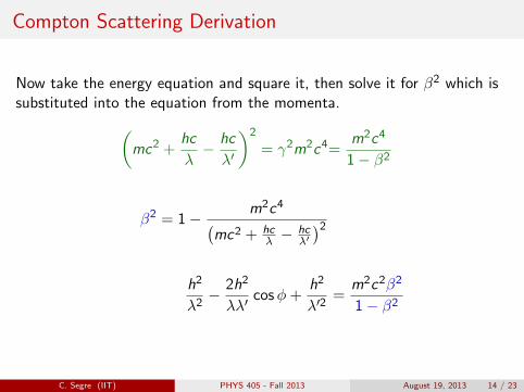
Compton Scattering Derivation
Now take the energy equation and square it, then solve it for β2 which issubstituted into the equation from the momenta.(
mc2 +hc
λ− hc
λ′
)2
= γ2m2c4=m2c4
1− β2
β2 = 1− m2c4(mc2 + hc
λ −hcλ′
)2h2
λ2− 2h2
λλ′cosφ+
h2
λ′2=
m2c2β2
1− β2
C. Segre (IIT) PHYS 405 - Fall 2013 August 19, 2013 14 / 23

Compton Scattering Derivation
After substitution, expansion and cancellation, we obtain
h2
λ2+
h2
λ′2− 2h2
λλ′cosφ = 2m
(hc
λ− hc
λ′
)+
h2
λ2+
h2
λ′2− 2h2
λλ′
2h2
λλ′(1− cosφ) = 2m
(hc
λ− hc
λ′
)= 2mhc
(λ′ − λλλ′
)=
2mhc∆λ
λλ′
∆λ =h
mc(1− cosφ)
C. Segre (IIT) PHYS 405 - Fall 2013 August 19, 2013 15 / 23

Compton Scattering Equation
∆λ =h
mc(1− cosφ)
C. Segre (IIT) PHYS 405 - Fall 2013 August 19, 2013 16 / 23

Davisson-Germer Experiment
In 1928, Davisson & Germershowed that DeBroglie’s hy-pothesis of the wave nature ofparticles.
By measuring the electronsscattered at various energiesfrom a metal foil, the observa-tion of Bragg’s Law for elec-trons was made.
This could only be explained byinterference between electrons.
C. Segre (IIT) PHYS 405 - Fall 2013 August 19, 2013 17 / 23

1D Schrodinger equation
i~∂Ψ
∂t= − ~2
2m
∂2Ψ
∂x2+ VΨ
i~∂Ψ
∂t= Total Energy
− ~2
2m
∂2Ψ
∂x2= Kinetic Energy
VΨ = Potential Energy
where the wave function,Ψ(x , t) is a function of bothtime and spacethis equation can be viewed asan expression of conservationof energy
C. Segre (IIT) PHYS 405 - Fall 2013 August 19, 2013 18 / 23

1D Schrodinger equation
i~∂Ψ
∂t= − ~2
2m
∂2Ψ
∂x2+ VΨ
i~∂Ψ
∂t= Total Energy
− ~2
2m
∂2Ψ
∂x2= Kinetic Energy
VΨ = Potential Energy
where the wave function,Ψ(x , t) is a function of bothtime and space
this equation can be viewed asan expression of conservationof energy
C. Segre (IIT) PHYS 405 - Fall 2013 August 19, 2013 18 / 23

1D Schrodinger equation
i~∂Ψ
∂t= − ~2
2m
∂2Ψ
∂x2+ VΨ
i~∂Ψ
∂t= Total Energy
− ~2
2m
∂2Ψ
∂x2= Kinetic Energy
VΨ = Potential Energy
where the wave function,Ψ(x , t) is a function of bothtime and spacethis equation can be viewed asan expression of conservationof energy
C. Segre (IIT) PHYS 405 - Fall 2013 August 19, 2013 18 / 23

1D Schrodinger equation
i~∂Ψ
∂t= − ~2
2m
∂2Ψ
∂x2+ VΨ
i~∂Ψ
∂t= Total Energy
− ~2
2m
∂2Ψ
∂x2= Kinetic Energy
VΨ = Potential Energy
where the wave function,Ψ(x , t) is a function of bothtime and spacethis equation can be viewed asan expression of conservationof energy
C. Segre (IIT) PHYS 405 - Fall 2013 August 19, 2013 18 / 23

Meaning of the wave function
The wave function, Ψ(x , t) de-scribes everything about a par-ticle (system)
a complex quantity but itsphase is meaningless
spatial integral gives probabilityof the particle being found inthe interval from a to b
Copenhagen interpretation hasproven to be correct one – col-lapse of the wave function aftermeasurement!
∫ b
a|Ψ(x , t)|2 dx
|Ψ|2
xa b
C. Segre (IIT) PHYS 405 - Fall 2013 August 19, 2013 19 / 23

Probability review
N =∞∑j=0
N(j)
P(j) =N(j)
N
1 =∞∑j=0
P(j)
〈j〉 =
∑jN(j)
N
=∞∑j=0
jP(j)
Suppose we have a distribution of discrete quantitiessuch as ages of people in a sports stadium, where N(j)is the number of individuals with the age j .
Thetotal number of people, N, is
The probability of an individual chosen at randomfrom the crowd having the age j is
The sum of all the probabilities must be 1
The average value of the age (not the most probable)is given by
C. Segre (IIT) PHYS 405 - Fall 2013 August 19, 2013 20 / 23

Probability review
N =∞∑j=0
N(j)
P(j) =N(j)
N
1 =∞∑j=0
P(j)
〈j〉 =
∑jN(j)
N
=∞∑j=0
jP(j)
Suppose we have a distribution of discrete quantitiessuch as ages of people in a sports stadium, where N(j)is the number of individuals with the age j . Thetotal number of people, N, is
The probability of an individual chosen at randomfrom the crowd having the age j is
The sum of all the probabilities must be 1
The average value of the age (not the most probable)is given by
C. Segre (IIT) PHYS 405 - Fall 2013 August 19, 2013 20 / 23

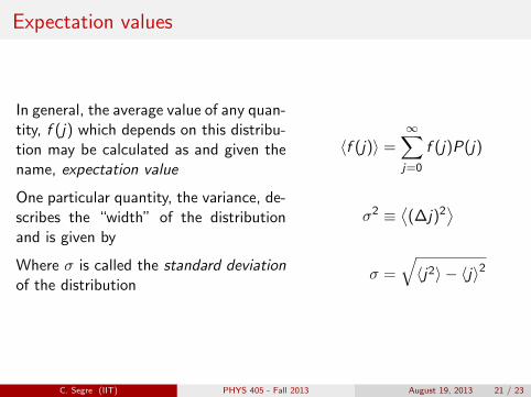
Expectation values
In general, the average value of any quan-tity, f (j) which depends on this distribu-tion may be calculated as
and given thename, expectation value
One particular quantity, the variance, de-scribes the “width” of the distributionand is given by
Where σ is called the standard deviationof the distribution
〈f (j)〉 =∞∑j=0
f (j)P(j)
σ2 ≡⟨(∆j)2
⟩σ =
√〈j2〉 − 〈j〉2
C. Segre (IIT) PHYS 405 - Fall 2013 August 19, 2013 21 / 23
Expectation values
In general, the average value of any quan-tity, f (j) which depends on this distribu-tion may be calculated as and given thename, expectation value
One particular quantity, the variance, de-scribes the “width” of the distributionand is given by
Where σ is called the standard deviationof the distribution
〈f (j)〉 =∞∑j=0
f (j)P(j)
σ2 ≡⟨(∆j)2
⟩σ =
√〈j2〉 − 〈j〉2
C. Segre (IIT) PHYS 405 - Fall 2013 August 19, 2013 21 / 23

Expectation values
In general, the average value of any quan-tity, f (j) which depends on this distribu-tion may be calculated as and given thename, expectation value
One particular quantity, the variance, de-scribes the “width” of the distributionand is given by
Where σ is called the standard deviationof the distribution
〈f (j)〉 =∞∑j=0
f (j)P(j)
σ2 ≡⟨(∆j)2
⟩
σ =
√〈j2〉 − 〈j〉2
C. Segre (IIT) PHYS 405 - Fall 2013 August 19, 2013 21 / 23
Expectation values
In general, the average value of any quan-tity, f (j) which depends on this distribu-tion may be calculated as and given thename, expectation value
One particular quantity, the variance, de-scribes the “width” of the distributionand is given by
Where σ is called the standard deviationof the distribution
〈f (j)〉 =∞∑j=0
f (j)P(j)
σ2 ≡⟨(∆j)2
⟩σ =
√〈j2〉 − 〈j〉2
C. Segre (IIT) PHYS 405 - Fall 2013 August 19, 2013 21 / 23
Computing the variance
σ2 =⟨(∆j)2
⟩
=∑
(∆j)2 P(j)
=∑
(j − 〈j〉)2 P(j)
=∑(
j2 − 2j 〈j〉+ 〈j〉2)P(j)
=∑
j2P(j) +∑
2j 〈j〉P(j) +∑〈j〉2 P(j)
=⟨j2⟩− 2 〈j〉 〈j〉+ 〈j〉2 =
⟨j2⟩− 〈j〉2
∆j = (j − 〈j〉)
expanding the square
dividing into threesums
Since σ2 ≥ 0,⟨j2⟩≥ 〈j〉2
C. Segre (IIT) PHYS 405 - Fall 2013 August 19, 2013 22 / 23

Computing the variance
σ2 =⟨(∆j)2
⟩=∑
(∆j)2 P(j)
=∑
(j − 〈j〉)2 P(j)
=∑(
j2 − 2j 〈j〉+ 〈j〉2)P(j)
=∑
j2P(j) +∑
2j 〈j〉P(j) +∑〈j〉2 P(j)
=⟨j2⟩− 2 〈j〉 〈j〉+ 〈j〉2
=⟨j2⟩− 〈j〉2
∆j = (j − 〈j〉)
expanding the square
dividing into threesums
Since σ2 ≥ 0,⟨j2⟩≥ 〈j〉2
C. Segre (IIT) PHYS 405 - Fall 2013 August 19, 2013 22 / 23

Computing the variance
σ2 =⟨(∆j)2
⟩=∑
(∆j)2 P(j)
=∑
(j − 〈j〉)2 P(j)
=∑(
j2 − 2j 〈j〉+ 〈j〉2)P(j)
=∑
j2P(j) +∑
2j 〈j〉P(j) +∑〈j〉2 P(j)
=⟨j2⟩− 2 〈j〉 〈j〉+ 〈j〉2 =
⟨j2⟩− 〈j〉2
∆j = (j − 〈j〉)
expanding the square
dividing into threesums
Since σ2 ≥ 0,⟨j2⟩≥ 〈j〉2
C. Segre (IIT) PHYS 405 - Fall 2013 August 19, 2013 22 / 23

Computing the variance
σ2 =⟨(∆j)2
⟩=∑
(∆j)2 P(j)
=∑
(j − 〈j〉)2 P(j)
=∑(
j2 − 2j 〈j〉+ 〈j〉2)P(j)
=∑
j2P(j) +∑
2j 〈j〉P(j) +∑〈j〉2 P(j)
=⟨j2⟩− 2 〈j〉 〈j〉+ 〈j〉2 =
⟨j2⟩− 〈j〉2
∆j = (j − 〈j〉)
expanding the square
dividing into threesums
Since σ2 ≥ 0,⟨j2⟩≥ 〈j〉2
C. Segre (IIT) PHYS 405 - Fall 2013 August 19, 2013 22 / 23

Continuous variables
We can extend all of these quantities to a system of continuous variables
with the introduction of the probability density, ρ(x) = |Ψ|2
P(j) =N(j)
Nρ(x)
1 =∞∑j=0
P(j) 1 =
∫ +∞
−∞ρ(x)dx
〈f (j)〉 =∞∑j=0
f (j)P(j) 〈f (x)〉 =
∫ +∞
−∞f (x)ρ(x)dx
σ2 ≡⟨(∆j)2
⟩=⟨j2⟩− 〈j〉2 σ2 ≡
⟨(∆x)2
⟩=⟨x2⟩− 〈x〉2
C. Segre (IIT) PHYS 405 - Fall 2013 August 19, 2013 23 / 23

Continuous variables
We can extend all of these quantities to a system of continuous variableswith the introduction of the probability density, ρ(x) = |Ψ|2
P(j) =N(j)
N
ρ(x)
1 =∞∑j=0
P(j) 1 =
∫ +∞
−∞ρ(x)dx
〈f (j)〉 =∞∑j=0
f (j)P(j) 〈f (x)〉 =
∫ +∞
−∞f (x)ρ(x)dx
σ2 ≡⟨(∆j)2
⟩=⟨j2⟩− 〈j〉2 σ2 ≡
⟨(∆x)2
⟩=⟨x2⟩− 〈x〉2
C. Segre (IIT) PHYS 405 - Fall 2013 August 19, 2013 23 / 23

Continuous variables
We can extend all of these quantities to a system of continuous variableswith the introduction of the probability density, ρ(x) = |Ψ|2
P(j) =N(j)
Nρ(x)
1 =∞∑j=0
P(j) 1 =
∫ +∞
−∞ρ(x)dx
〈f (j)〉 =∞∑j=0
f (j)P(j) 〈f (x)〉 =
∫ +∞
−∞f (x)ρ(x)dx
σ2 ≡⟨(∆j)2
⟩=⟨j2⟩− 〈j〉2 σ2 ≡
⟨(∆x)2
⟩=⟨x2⟩− 〈x〉2
C. Segre (IIT) PHYS 405 - Fall 2013 August 19, 2013 23 / 23

Continuous variables
We can extend all of these quantities to a system of continuous variableswith the introduction of the probability density, ρ(x) = |Ψ|2
P(j) =N(j)
Nρ(x)
1 =∞∑j=0
P(j)
1 =
∫ +∞
−∞ρ(x)dx
〈f (j)〉 =∞∑j=0
f (j)P(j) 〈f (x)〉 =
∫ +∞
−∞f (x)ρ(x)dx
σ2 ≡⟨(∆j)2
⟩=⟨j2⟩− 〈j〉2 σ2 ≡
⟨(∆x)2
⟩=⟨x2⟩− 〈x〉2
C. Segre (IIT) PHYS 405 - Fall 2013 August 19, 2013 23 / 23

Continuous variables
We can extend all of these quantities to a system of continuous variableswith the introduction of the probability density, ρ(x) = |Ψ|2
P(j) =N(j)
Nρ(x)
1 =∞∑j=0
P(j) 1 =
∫ +∞
−∞ρ(x)dx
〈f (j)〉 =∞∑j=0
f (j)P(j) 〈f (x)〉 =
∫ +∞
−∞f (x)ρ(x)dx
σ2 ≡⟨(∆j)2
⟩=⟨j2⟩− 〈j〉2 σ2 ≡
⟨(∆x)2
⟩=⟨x2⟩− 〈x〉2
C. Segre (IIT) PHYS 405 - Fall 2013 August 19, 2013 23 / 23

Continuous variables
We can extend all of these quantities to a system of continuous variableswith the introduction of the probability density, ρ(x) = |Ψ|2
P(j) =N(j)
Nρ(x)
1 =∞∑j=0
P(j) 1 =
∫ +∞
−∞ρ(x)dx
〈f (j)〉 =∞∑j=0
f (j)P(j)
〈f (x)〉 =
∫ +∞
−∞f (x)ρ(x)dx
σ2 ≡⟨(∆j)2
⟩=⟨j2⟩− 〈j〉2 σ2 ≡
⟨(∆x)2
⟩=⟨x2⟩− 〈x〉2
C. Segre (IIT) PHYS 405 - Fall 2013 August 19, 2013 23 / 23

Continuous variables
We can extend all of these quantities to a system of continuous variableswith the introduction of the probability density, ρ(x) = |Ψ|2
P(j) =N(j)
Nρ(x)
1 =∞∑j=0
P(j) 1 =
∫ +∞
−∞ρ(x)dx
〈f (j)〉 =∞∑j=0
f (j)P(j) 〈f (x)〉 =
∫ +∞
−∞f (x)ρ(x)dx
σ2 ≡⟨(∆j)2
⟩=⟨j2⟩− 〈j〉2 σ2 ≡
⟨(∆x)2
⟩=⟨x2⟩− 〈x〉2
C. Segre (IIT) PHYS 405 - Fall 2013 August 19, 2013 23 / 23

Continuous variables
We can extend all of these quantities to a system of continuous variableswith the introduction of the probability density, ρ(x) = |Ψ|2
P(j) =N(j)
Nρ(x)
1 =∞∑j=0
P(j) 1 =
∫ +∞
−∞ρ(x)dx
〈f (j)〉 =∞∑j=0
f (j)P(j) 〈f (x)〉 =
∫ +∞
−∞f (x)ρ(x)dx
σ2 ≡⟨(∆j)2
⟩=⟨j2⟩− 〈j〉2
σ2 ≡⟨(∆x)2
⟩=⟨x2⟩− 〈x〉2
C. Segre (IIT) PHYS 405 - Fall 2013 August 19, 2013 23 / 23

Continuous variables
We can extend all of these quantities to a system of continuous variableswith the introduction of the probability density, ρ(x) = |Ψ|2
P(j) =N(j)
Nρ(x)
1 =∞∑j=0
P(j) 1 =
∫ +∞
−∞ρ(x)dx
〈f (j)〉 =∞∑j=0
f (j)P(j) 〈f (x)〉 =
∫ +∞
−∞f (x)ρ(x)dx
σ2 ≡⟨(∆j)2
⟩=⟨j2⟩− 〈j〉2 σ2 ≡
⟨(∆x)2
⟩=⟨x2⟩− 〈x〉2
C. Segre (IIT) PHYS 405 - Fall 2013 August 19, 2013 23 / 23