Embed Size (px)
Citation preview
Physical Mechanisms of the Wintertime Surface Air Temperature Variabilityin South Korea and the near-7-Day Oscillations
KWANG-YUL KIM AND JOON-WOO ROH
School of Earth and Environmental Sciences, Seoul National University, Seoul, South Korea
(Manuscript received 14 July 2009, in final form 17 November 2009)
ABSTRACT
The first three principal modes of wintertime surface temperature variability in Seoul, South Korea
(37.338N, 126.598E), are extracted from the 1979–2008 observed records via cyclostationary EOF (CSEOF)
analysis. The first mode represents the seasonal cycle, the principle physical mechanism of which is associated
with the continent–ocean sea level pressure contrast. The second mode mainly describes the overall win-
tertime warming or cooling. The third mode depicts subseasonal fluctuations of surface temperature. Sea level
pressure anomalies to the west of South Korea (eastern China) and those with an opposite sign to the east of
South Korea (Japan) are a major physical factor both for the second mode and the third mode. These sea level
pressure anomalies with opposite signs alter the amount of warm air to the south of South Korea, which
changes the surface temperature in South Korea. The PC time series of the seasonal cycle is significantly
correlated with the East Asian winter monsoon index and exhibits a conspicuous downward trend. The PC
time series of the second mode exhibits a positive trend. These trends imply that the wintertime surface
temperature in South Korea has increased and the seasonal cycle has weakened gradually over the past 30 yr;
the sign of greenhouse warming is clear in both PC time series.
The ;7-day oscillations are a major component of high-frequency variability in much of the analysis
domain and are a manifestation of Rossby waves. Rossby waves aloft result in the concerted variation of
physical variables in the atmospheric column. Due to the stronger mean zonal wind, the disturbances by
Rossby waves propagate eastward at ;8–12 m s21; the passing of Rossby waves with alternating signs pro-
duces the ;7-day temperature oscillations in South Korea.
1. Introduction
One of the strongest manifestations of greenhouse
warming in South Korea is the increasing wintertime sur-
face temperature (Ryoo et al. 2004). Although the ob-
servation records clearly show this warming, a detailed
examination or explanation of the nature of this warm-
ing has not been attempted in any serious manner. It
is extremely important to understand how the increas-
ing concentration of greenhouse gases alters the winter-
time physical mechanisms in South Korea and how the
changing physical mechanisms, in turn, alter the surface
temperature in South Korea.
On a short time scale, short waves propagating in the
northwesterly flow initiate descent in the region of the East
Asian coast. The divergent outflow from and the circula-
tion about the center of the disturbance thrust cold air
southward. These short waves usually initiate rapid cy-
clogenesis in the highly baroclinic flow off the Korean
Peninsula (Boyle 1986).
Cold surges are one of the dominant wintertime fea-
tures in South Korea. A composite of six individual cold-
air outbreaks over South Korea during 1985–86 shows
that the development of a surge over South Korea is pre-
ceded by a ridge to the west of Lake Baikal and a trough
over the East Asian coast (Boyle 1986; Park and Kim
1987). This wavelike disturbance accompanied by a cold-
air outbreak experiences a systematic structural change
as it propagates southeastward with a phase speed of
;108 day21 from Lake Baikal toward South Korea. This
wave, with a cold trough and a warm ridge, is typically
characterized by a wavelength of about 4000 km (Park
and Kim 1987). Active transient disturbances—a zone of
strong baroclinicity—develop over East Asia near the
downstream region of the climatological jet during cold
surges (Blackmon et al. 1977). The cold surge circulation
has a strong effect on the zonal momentum budget in the
Corresponding author address: Kwang-Yul Kim, School of Earth
and Environmental Sciences, Seoul National University, San 56-1,
Shillim-dong, Gwanak-gu, Seoul 151-747, South Korea.
E-mail: [email protected]
15 APRIL 2010 K I M A N D R O H 2197
DOI: 10.1175/2009JCLI3348.1
� 2010 American Meteorological Society
vicinity of the maximum East Asian jet (Boyle 1986). A
composite of cold surge events also showed that an upper-
level baroclinic wave of ;608 wavelength propagates
eastward from the west of Lake Baikal toward the eastern
coast of China with a phase speed of 128 day21 causing
a cold-air outbreak in South Korea (Ryoo et al. 2005).
Cold surges during winter not only dominate local
weather but also have a strong impact on the extratrop-
ical and tropical planetary-scale circulations in East Asia
(Chang and Lau 1982). The East Asian cold surge has
been studied as one of most conspicuous features of the
Asian winter monsoon. Cold surges along the south
China coast enhance the local Hadley circulation over
East Asia by strengthening cold advection over northern
China, which in turn causes additional upper-level di-
vergence over the equatorial South China Sea (Chang
et al. 1979; Chang and Lau 1980, 1982; Chu and Park
1984).
In contrast to daily weather changes in the middle
latitudes, which are mostly characterized by baroclinic
disturbances, the causes of low-frequency atmospheric
variability are not well understood (Wallace and Blackmon
1983). During the winter monsoon, it is frequently ob-
served that a huge anticyclone over Siberia dominates
the low-level circulation over Asia, giving rise to strong
northerly and northeasterly winds covering the entire
region of central and northern China and the South China
Sea. Indeed, the variability of the wintertime temperature
in South Korea on a monthly temporal scale is roughly
explained in terms of the strength of the Siberian high and
the Aleutian low. Cold winters are accompanied by the
intensification of the Siberian high and/or the Aleutian
low, which develops a stronger East Asian jet in the upper
troposphere (Kang 1988; Ryoo et al. 2002; Yang et al.
2002). Under these conditions, the monthly winter tem-
perature in South Korea is significantly influenced by
stronger lower-tropospheric northerly monsoonal flow
over the eastern coast of Asia (Kang 1988; Yang et al.
2002). In fact, the intensification of the Siberian high and
the Aleutian low is positively correlated with the winter
temperature in South Korea (Ryoo et al. 2002).
While some of physical mechanisms that lead to sur-
face temperature variability on various time scales have
been investigated, it is largely unknown how greenhouse
warming affects these physical mechanisms. Thus, the
primary focus of this study is on understanding the physical
mechanisms associated with the variability of the win-
tertime surface temperature in South Korea. Specifically,
this study attempts to address how greenhouse warming
manifests itself in different physical processes governing
wintertime surface temperature variations. The physical
mechanism of the ;7-day oscillations, also called the
three-cold-day/four-warm-day events, is also investigated
in order to address if greenhouse warming caused any
changes in either the magnitude or the nature of this par-
ticular phenomenon.
The data employed in this study are described in sec-
tion 2, followed by a description of the CSEOF analysis,
which is the major analysis tool in the present study, and
the regression technique, which is used to extract phys-
ically consistent patterns of key variables. The latter
technique is used to understand the physical mechanism
of the major modes of surface temperature variability
and the ;7-day oscillations. The results of the analysis
are discussed in section 4 with specific emphasis on the
physical nature of the surface temperature variability in
South Korea. Concluding remarks and the summary are
presented in section 5.
2. Data
The 30-yr (1979–2008) observations of surface tem-
peratures in Seoul, South Korea (37.338N, 126.598E),
were acquired from the Korea Meteorological Adminis-
tration. The data are from a daily averaged time series
at a station in Seoul. Then, 2.58 3 2.58 arrays of daily
temperatures, geopotential heights, and winds at stan-
dard levels from 1000 to 200 hPa were extracted from
the daily National Centers for Environmental Prediction–
National Center for Atmospheric Research (NCEP–
NCAR) reanalysis dataset for the same period (Kalnay
et al. 1996). In addition to these data, daily NCEP–
NCAR 2-m air temperature and 10-m wind were used
in the analysis; they come at a zonal resolution of 1.8758
with 94 Gaussian levels in the meridional direction. The
potential vorticity (PV) was calculated by first calculating
potential temperature u in the form
u 5 T( ps/p)R/C
p , (1)
where R is the universal gas constant and cp is the specific
heat capacity at constant pressure. Then, PV is given by
y 5�g( f 1 z)›u
›p, (2)
where (2) was evaluated using finite differencing be-
tween two adjacent pressure levels.
To investigate the wintertime variability, 120 days from
17 November through 16 March were taken from each
winter for the 29 winter seasons in the record. Thus,
each year represents 120 winter days. For leap years,
29 February was averaged with 28 February to have a
nested period of exactly 120 days. The same 120 winter
days were used for all the datasets employed in the
present study. The analysis domain is composed of East
2198 J O U R N A L O F C L I M A T E VOLUME 23
Asia (22.58–72.58N, 97.58–152.58E) for all the variables
except PV. The PV data were analyzed over the entire
zonal band extending from 308 to 808N; this is to facilitate
the computation of zonal wavenumbers of Rossby waves.
3. Method
a. CSEOF analysis
To separate the physical processes from the datasets,
the CSEOF technique was employed (Kim et al. 1996;
Kim and North 1997). In this method, space–time data,
T(r, t), are written as a linear superposition of the
CSEOFs:
T(r, t) 5 �n
LVn(r, t)PC
n(t), (3)
where LVn(r, t) and PCn(t) are cyclostationary loading
vectors and principal component (PC) time series, re-
spectively. The CSEOF representation of the data is dif-
ferent from the EOF representation in that the loading
vectors are time dependent and periodic; that is,
LVn(r, t) 5 LV
n(r, t 1 d), (4)
where d is called the nested period. It is emphasized that
the CSEOF loading vectors represent temporally evolv-
ing physical processes, whereas the PC time series rep-
resent the amplitude modulation of the physical processes
on longer time scales. Examples of physical and dynam-
ical interpretations of CSEOFs can be found in the recent
literature (Seo and Kim 2003; Kullgren and Kim 2006;
Kim et al. 2006; Lim and Kim 2007).
The nested period, d, represents the periodicity of the
space–time covariance function and is associated with
the inherent time scales of the physical processes. As can
be seen in (4), the nested period should be long enough
to include all of the different periods of the physical
processes in the dataset; in fact, it should be the least
common multiple of all of the different physical periods
in a given dataset. In this study, the nested period is as-
sumed to be 1 yr; this implies that the statistical proper-
ties of each physical process do not vary from one year to
another although realizations of a physical process vary
from one year to another. The nested period is an im-
portant caveat for the CSEOF technique. Nonetheless,
finding a suitable nested period has not posed any seri-
ous problem in applying the CSEOF technique as dem-
onstrated in the papers addressed above.
b. Regression analysis
To understand the detailed physical nature of physical
processes, many important physical variables will be sub-
ject to CSEOF analysis in the present study. This means
that physically and dynamically consistent patterns should
be derived from many variables. This is accomplished in
the following manner. A CSEOF analysis is conducted
on each physical variable. Then, the PC time series of
a target variable (say, temperature) is written as a linear
regression of the PC time series of a predictor variable
(say, sea level pressure). That is,
PCTi(t) 5 �
na(i)
n PCn(t) 1 «(t), (5)
where PCTi(t) is the target PC time series for mode i,
PCn(t) is the predictor time series for mode n, and «(t)
is the regression error time series. The regression co-
efficients a(i)n are determined such that the variance of the
regression error time series is minimized. The degree of
fitting for each mode is measured by r 2i 5 1� var[«(t)]/
var[PCTi(t)].
Then, the spatiotemporal pattern of the predictor var-
iable, LVPi(r, t), which is consistent with the pattern of
the target variable, LVTi(r, t), is obtained by
LVPi(r, t) 5 �
na(i)
n LVn(r, t), (6)
where LVn(r, t) are the CSEOF loading vectors of the
predictor variable. Note that LVTi(r, t) and LVPi(r, t)
are called physically and dynamically consistent within
the context of having (nearly) identical amplitude time
series, not because of the identical physical evolution.
In fact, the spatiotemporal evolution in LVTi(r, t) and
LVPi(r, t) may, in general, be very different from each
other. Note, on the other hand, that LVTi(r, t) and
LVPi(r, t) have nearly identical amplitude time series.
This regression method is equivalent to the so-called
projection method when it is applied to EOFs.
4. Results and discussion
Modes of fluctuations of surface air temperature in
Seoul have been identified via CSEOF analysis. CSEOF
analysis on the wintertime surface air temperature ex-
tracts three principal modes of variability, which to-
gether explain about 50% of the total variability. In this
section, physical and dynamical mechanisms of surface
air temperature variability will be investigated based on
the first three CSEOF modes extracted from the ob-
servational data.
CSEOF analysis has also been conducted on the 2-m
surface air temperatures of the NCEP–NCAR daily re-
analysis product over the same time interval. Then, re-
gression analysis has been performed as described earlier
using 20 predictor modes to identify physical evolution
patterns in space and in time associated with the first
three principle modes of variability of the wintertime
15 APRIL 2010 K I M A N D R O H 2199
surface air temperatures in Seoul. Similarly, evolution-
ary patterns of different physical variables were identi-
fied to be consistent with each CSEOF of the observed
surface air temperature in Seoul. As a check of the va-
lidity of the regressed surface air temperature patterns,
the physical evolution pattern at 37.58N, 127.58E, the
grid point closest to Seoul, was compared with that of
the observed time series for the first three modes. The
correlations are 0.954, 0.883, and 0.889 for the first three
modes, respectively (see Figs. 1, 3, and 7). Thus, the re-
gressed surface air temperature patterns appear to be
reasonably consistent with the observed time series in
Seoul.
a. The seasonal cycle
CSEOF analysis extracts the seasonal cycle as the first
mode of variability, as expected. This mode explains
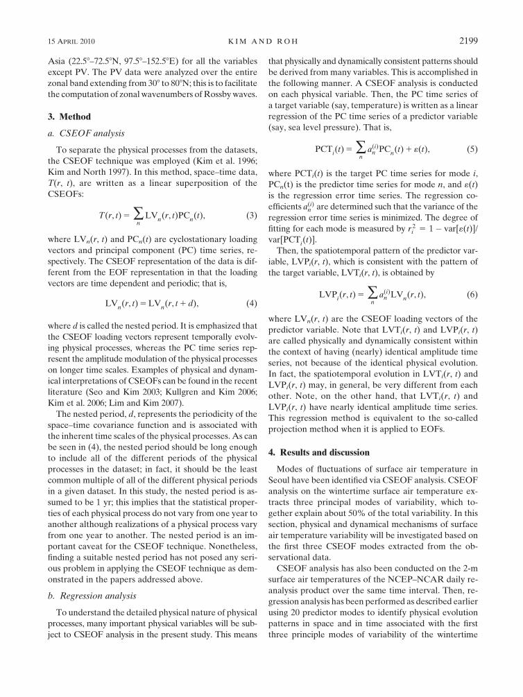
;33% of the total variability. Figure 1a shows the sea-
sonal cycle of the temperature during the 120 winter days
(17 November–16 March) in Seoul as identified from the
actual observational data. As can be seen, the surface air
temperature in Seoul is at its minimum typically be-
tween the end of January and the early February. The
corresponding PC time series shows remarkable inter-
annual fluctuations in the amplitude of the seasonal cy-
cle (Fig. 1b). The period of the maximum spectral peak
is ;4 yr (figure not shown). The amplitude of the sea-
sonal cycle fluctuates significantly; Figs. 1a and 1b imply
that the range of surface temperature variations during
the wintertime in association with the seasonal cycle is
approximately between 48 and 198.
There is an interesting trend in the PC time series with
a slope of 20.0371 yr21 and an estimated error standard
deviation of 0.0012. This trend cannot be rejected even
at a 99% level; thus, the trend appears to be real. This
trend indicates that the strength of the seasonal cycle has
steadily decreased at the rate of about 1 unit per 30 years
(see Fig. 1b). This implies that the difference between
a maximum temperature and a minimum temperature
during a winter season as shown in Fig. 1a has been de-
creasing in the mean sense although there are significant
year-to-year variations, as shown in Fig. 1b.
Figure 2 shows the patterns of 2-m air temperature,
sea level pressure, and 10-m wind that exhibit the same
evolution as that of the surface air temperature in Seoul,
shown in Fig. 1a. These patterns were obtained by pro-
jecting the regressed evolution of the physical variables
onto the evolution of the surface air temperature in Seoul,
as shown in Fig. 1a. The time series of the regressed 2-m
air temperatures at a grid point closest to Seoul is corre-
lated at 0.954 with the surface air temperature in Seoul,
as shown in Fig. 1a. Temperature variations in Seoul as
reflected in the seasonal cycle are associated with a gen-
eral warming–cooling over the entire continental domain
considered here (Fig. 2). A positive surface temperature
anomaly in Seoul is associated with negative sea level
pressure anomalies over the Asian continent and posi-
tive sea level pressure anomalies over the northwest Pa-
cific. As a result, southeasterly wind anomalies develop
strongly to the south of South Korea, transporting warm
air into Seoul. A weakening seasonal cycle implies that
the evolution of the patterns of physical variables shown
in Fig. 2 from a positive phase to a negative one during
winter, on average, has weakened in recent years.
Figure 2 depicts typical patterns of physical variables
associated with the East Asian winter monsoon. In fact,
the PC time series in Fig. 1b is highly correlated with the
East Asian winter monsoon index (Jhun and Lee 2004).
This confirms that the seasonal cycle of surface air tem-
perature in Seoul is strongly influenced by the strength
of the East Asian winter monsoon, which, in turn, is
controlled by the contrasting sea level pressure anom-
alies between the continent and the ocean.
b. The second CSEOF mode: The subseasonal mode
The second mode describes the wintertime subseasonal
fluctuations of surface air temperature in Seoul and ex-
plains ;11% of the total variability (Fig. 3a). As shown
in Fig. 3, submonthly fluctuations are obvious on top
of lower-frequency undulations. The corresponding
PC time series shows that there is a noticeable upward
trend with a slope of 0.0676 yr21 and an estimated error
FIG. 1. (a) The wintertime (17 Nov–16 Mar) seasonal cycle of the
surface air temperature in Seoul (solid line). The corresponding
evolution of the regressed NCEP–NCAR 2-m surface air temper-
ature at the nearest grid point (dotted line). Correlation is 0.954
between the two time series. (b) The amplitude time series of the
wintertime seasonal cycle of the surface air temperature.
2200 J O U R N A L O F C L I M A T E VOLUME 23

standard deviation of 0.0029 (Fig. 3b); the trend is sig-
nificant at the 99% level. According to the PC time se-
ries, the amplitude of this particular mode tends to be
positive more often recently than 30 yr ago. This implies
that the wintertime surface air temperature tends to be
warmer recently than previously since the evolution
pattern in Fig. 3a depicts primarily a warming in Seoul
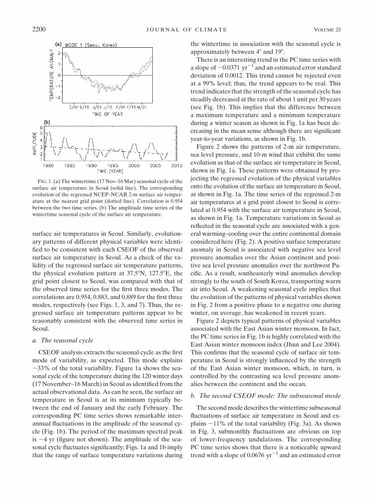
throughout the winter. In fact, the reconstruction of the
surface temperatures in Seoul using the first two modes
shows that the average temperature between 15 January
and 15 February has risen by ;38 in the past 30 yr, which
is consistent with the estimate based on the actual ob-
servational data (Fig. 4). The corresponding best auto-
regressive (AR) spectrum indicates the maximum spectral
peak at ;4 yr. Thus, the wintertime average surface air
temperature in Seoul fluctuates with approximately a
4-yr period.
Correlations between the evolution pattern of the re-
gressed 2-m air temperature in Seoul (conveniently at
37.58N, 127.58E) and the loading vectors of the regressed
variables were computed at each grid point for the sec-
ond mode. Correlations were computed up to the lag of
67 days to investigate the lead–lag relationship between
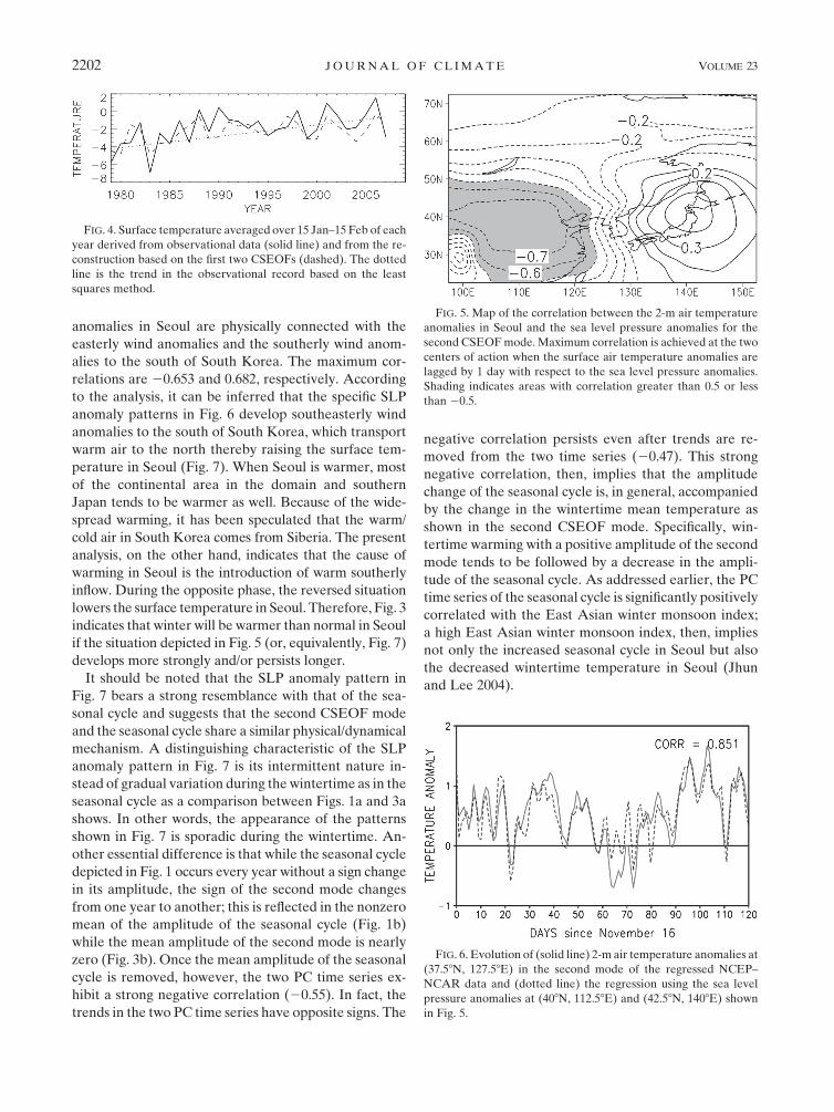
the two variables. Figure 5 shows a map of the correla-
tion between the 2-m air temperature anomalies and the
sea level pressure anomalies for the second CSEOF
mode. The correlation is strongest when the sea level
pressure leads the 2-m air temperature in Seoul by 1 day.
There are two distinct centers of action: one located over
eastern China (408N, 112.58E) and the other over north-
eastern Japan (42.58N, 1408E). Figure 5 indicates that, in
general, negative sea level pressure anomalies are ob-
served over eastern China and positive sea level pres-
sure anomalies are observed over Japan in conjunction
with positive surface air temperature anomalies in Seoul.
The sea level pressure change over eastern China exerts
a stronger influence on the surface air temperature in
Seoul than that over Japan.
Figure 6 shows the connection between the 2-m air
temperature anomalies at 37.58N, 127.58E and the sea
level pressure anomalies at 408N, 112.58E and 42.58N,
1408E associated with the second mode; the 2-m air
temperature anomalies at 37.58N, 127.58E are reason-
ably regressed in terms of the two SLP anomalies at
408N, 112.58E and 42.58N, 1408E. As shown in Fig. 6, the
physical connection between the surface temperature
anomalies in Seoul and the SLP anomalies in Fig. 5 is
obvious (r 5 0.845), showing clearly that the change in
surface air temperature in Seoul is related to the de-
velopment of the two opposite SLP anomaly patterns
in Fig. 5.
Similar analysis with the zonal and meridional wind
anomalies shows further that the 2-m air temperature
FIG. 2. Map of (a) 2-m air temperature (light shading .0.58C; dark shading .1.08C) and
(b) sea level pressure and 10-m wind (light shading ,20.1 hPa; dark shading .0.1 hPa) as-
sociated with the evolution of the surface air temperature in Fig. 1. For clarity of exposition,
wind vectors of magnitude less than 0.1 m s21 are not shown.
FIG. 3. (a) The second CSEOF mode of the wintertime surface
air temperature in Seoul (solid line) and the corresponding evo-
lution of the regressed NCEP–NCAR 2-m surface air temperature
at the nearest grid point (dotted line). Correlation is 0.883 between
the two time series. (b) The amplitude time series of the second
CSEOF mode of the wintertime surface air temperature.
15 APRIL 2010 K I M A N D R O H 2201
anomalies in Seoul are physically connected with the
easterly wind anomalies and the southerly wind anom-
alies to the south of South Korea. The maximum cor-
relations are 20.653 and 0.682, respectively. According
to the analysis, it can be inferred that the specific SLP
anomaly patterns in Fig. 6 develop southeasterly wind
anomalies to the south of South Korea, which transport
warm air to the north thereby raising the surface tem-
perature in Seoul (Fig. 7). When Seoul is warmer, most
of the continental area in the domain and southern
Japan tends to be warmer as well. Because of the wide-
spread warming, it has been speculated that the warm/
cold air in South Korea comes from Siberia. The present
analysis, on the other hand, indicates that the cause of
warming in Seoul is the introduction of warm southerly
inflow. During the opposite phase, the reversed situation
lowers the surface temperature in Seoul. Therefore, Fig. 3
indicates that winter will be warmer than normal in Seoul
if the situation depicted in Fig. 5 (or, equivalently, Fig. 7)
develops more strongly and/or persists longer.
It should be noted that the SLP anomaly pattern in
Fig. 7 bears a strong resemblance with that of the sea-
sonal cycle and suggests that the second CSEOF mode
and the seasonal cycle share a similar physical/dynamical
mechanism. A distinguishing characteristic of the SLP
anomaly pattern in Fig. 7 is its intermittent nature in-
stead of gradual variation during the wintertime as in the
seasonal cycle as a comparison between Figs. 1a and 3a
shows. In other words, the appearance of the patterns
shown in Fig. 7 is sporadic during the wintertime. An-
other essential difference is that while the seasonal cycle
depicted in Fig. 1 occurs every year without a sign change
in its amplitude, the sign of the second mode changes
from one year to another; this is reflected in the nonzero
mean of the amplitude of the seasonal cycle (Fig. 1b)
while the mean amplitude of the second mode is nearly
zero (Fig. 3b). Once the mean amplitude of the seasonal
cycle is removed, however, the two PC time series ex-
hibit a strong negative correlation (20.55). In fact, the
trends in the two PC time series have opposite signs. The
negative correlation persists even after trends are re-
moved from the two time series (20.47). This strong
negative correlation, then, implies that the amplitude
change of the seasonal cycle is, in general, accompanied
by the change in the wintertime mean temperature as
shown in the second CSEOF mode. Specifically, win-
tertime warming with a positive amplitude of the second
mode tends to be followed by a decrease in the ampli-
tude of the seasonal cycle. As addressed earlier, the PC
time series of the seasonal cycle is significantly positively
correlated with the East Asian winter monsoon index;
a high East Asian winter monsoon index, then, implies
not only the increased seasonal cycle in Seoul but also
the decreased wintertime temperature in Seoul (Jhun
and Lee 2004).
FIG. 4. Surface temperature averaged over 15 Jan–15 Feb of each
year derived from observational data (solid line) and from the re-
construction based on the first two CSEOFs (dashed). The dotted
line is the trend in the observational record based on the least
squares method.
FIG. 5. Map of the correlation between the 2-m air temperature
anomalies in Seoul and the sea level pressure anomalies for the
second CSEOF mode. Maximum correlation is achieved at the two
centers of action when the surface air temperature anomalies are
lagged by 1 day with respect to the sea level pressure anomalies.
Shading indicates areas with correlation greater than 0.5 or less
than 20.5.
FIG. 6. Evolution of (solid line) 2-m air temperature anomalies at
(37.58N, 127.58E) in the second mode of the regressed NCEP–
NCAR data and (dotted line) the regression using the sea level
pressure anomalies at (408N, 112.58E) and (42.58N, 1408E) shown
in Fig. 5.
2202 J O U R N A L O F C L I M A T E VOLUME 23
Further examination of the corresponding loading vec-
tors indicates that the SLP pattern in Fig. 7 does not show
any significant sign of propagation. Thus, the patterns of
SLP anomalies and wind anomalies shown in Figs. 5 and
7 are essentially standing anomaly patterns. Figure 3b
indicates that the average wintertime temperature has
steadily increased in the past three decades with lower
SLPs over the continent and higher SLPs over the north-
western Pacific. The positive trend in Fig. 3b has not risen
above the level of natural variability but its presence is
confirmed at a 99% confidence level.
c. The third CSEOF mode: The intraseasonal mode
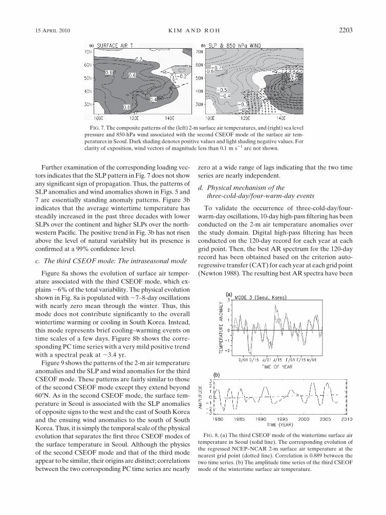
Figure 8a shows the evolution of surface air temper-
ature associated with the third CSEOF mode, which ex-
plains ;6% of the total variability. The physical evolution
shown in Fig. 8a is populated with ;7–8-day oscillations
with nearly zero mean through the winter. Thus, this
mode does not contribute significantly to the overall
wintertime warming or cooling in South Korea. Instead,
this mode represents brief cooling–warming events on
time scales of a few days. Figure 8b shows the corre-
sponding PC time series with a very mild positive trend
with a spectral peak at ;3.4 yr.
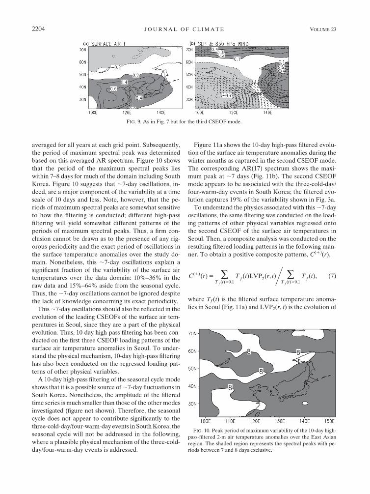
Figure 9 shows the patterns of the 2-m air temperature
anomalies and the SLP and wind anomalies for the third
CSEOF mode. These patterns are fairly similar to those
of the second CSEOF mode except they extend beyond
608N. As in the second CSEOF mode, the surface tem-
perature in Seoul is associated with the SLP anomalies
of opposite signs to the west and the east of South Korea
and the ensuing wind anomalies to the south of South
Korea. Thus, it is simply the temporal scale of the physical
evolution that separates the first three CSEOF modes of
the surface temperature in Seoul. Although the physics
of the second CSEOF mode and that of the third mode
appear to be similar, their origins are distinct; correlations
between the two corresponding PC time series are nearly
zero at a wide range of lags indicating that the two time
series are nearly independent.
d. Physical mechanism of thethree-cold-day/four-warm-day events
To validate the occurrence of three-cold-day/four-
warm-day oscillations, 10-day high-pass filtering has been
conducted on the 2-m air temperature anomalies over
the study domain. Digital high-pass filtering has been
conducted on the 120-day record for each year at each
grid point. Then, the best AR spectrum for the 120-day
record has been obtained based on the criterion auto-
regressive transfer (CAT) for each year at each grid point
(Newton 1988). The resulting best AR spectra have been
FIG. 7. The composite patterns of the (left) 2-m surface air temperatures, and (right) sea level
pressure and 850-hPa wind associated with the second CSEOF mode of the surface air tem-
peratures in Seoul. Dark shading denotes positive values and light shading negative values. For
clarity of exposition, wind vectors of magnitude less than 0.1 m s21 are not shown.
FIG. 8. (a) The third CSEOF mode of the wintertime surface air
temperature in Seoul (solid line). The corresponding evolution of
the regressed NCEP–NCAR 2-m surface air temperature at the
nearest grid point (dotted line). Correlation is 0.889 between the
two time series. (b) The amplitude time series of the third CSEOF
mode of the wintertime surface air temperature.
15 APRIL 2010 K I M A N D R O H 2203
averaged for all years at each grid point. Subsequently,
the period of maximum spectral peak was determined
based on this averaged AR spectrum. Figure 10 shows
that the period of the maximum spectral peaks lies
within 7–8 days for much of the domain including South
Korea. Figure 10 suggests that ;7-day oscillations, in-
deed, are a major component of the variability at a time
scale of 10 days and less. Note, however, that the pe-
riods of maximum spectral peaks are somewhat sensitive
to how the filtering is conducted; different high-pass
filtering will yield somewhat different patterns of the
periods of maximum spectral peaks. Thus, a firm con-
clusion cannot be drawn as to the presence of any rig-
orous periodicity and the exact period of oscillations in
the surface temperature anomalies over the study do-
main. Nonetheless, this ;7-day oscillations explain a
significant fraction of the variability of the surface air
temperatures over the data domain: 10%–36% in the
raw data and 15%–64% aside from the seasonal cycle.
Thus, the ;7-day oscillations cannot be ignored despite
the lack of knowledge concerning its exact periodicity.
This ;7-day oscillations should also be reflected in the
evolution of the leading CSEOFs of the surface air tem-
peratures in Seoul, since they are a part of the physical
evolution. Thus, 10-day high-pass filtering has been con-
ducted on the first three CSEOF loading patterns of the
surface air temperature anomalies in Seoul. To under-
stand the physical mechanism, 10-day high-pass filtering
has also been conducted on the regressed loading pat-
terns of other physical variables.
A 10-day high-pass filtering of the seasonal cycle mode
shows that it is a possible source of ;7-day fluctuations in
South Korea. Nonetheless, the amplitude of the filtered
time series is much smaller than those of the other modes
investigated (figure not shown). Therefore, the seasonal
cycle does not appear to contribute significantly to the
three-cold-day/four-warm-day events in South Korea; the
seasonal cycle will not be addressed in the following,
where a plausible physical mechanism of the three-cold-
day/four-warm-day events is addressed.
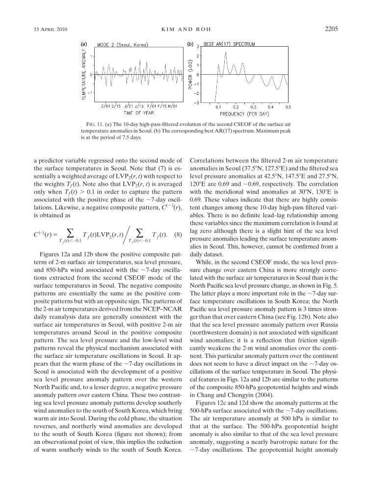
Figure 11a shows the 10-day high-pass filtered evolu-
tion of the surface air temperature anomalies during the
winter months as captured in the second CSEOF mode.
The corresponding AR(17) spectrum shows the maxi-
mum peak at ;7 days (Fig. 11b). The second CSEOF
mode appears to be associated with the three-cold-day/
four-warm-day events in South Korea; the filtered evo-
lution captures 19% of the variability shown in Fig. 3a.
To understand the physics associated with this ;7-day
oscillations, the same filtering was conducted on the load-
ing patterns of other physical variables regressed onto
the second CSEOF of the surface air temperatures in
Seoul. Then, a composite analysis was conducted on the
resulting filtered loading patterns in the following man-
ner. To obtain a positive composite patterns, C(1)(r),
C(1)(r) 5 �T
f(t).0.1
Tf(t)LVP
2(r, t) �
Tf(t).0.1
Tf(t),
,(7)
where Tf (t) is the filtered surface temperature anoma-
lies in Seoul (Fig. 11a) and LVP2(r, t) is the evolution of
FIG. 9. As in Fig. 7 but for the third CSEOF mode.
FIG. 10. Peak period of maximum variability of the 10-day high-
pass-filtered 2-m air temperature anomalies over the East Asian
region. The shaded region represents the spectral peaks with pe-
riods between 7 and 8 days exclusive.
2204 J O U R N A L O F C L I M A T E VOLUME 23
a predictor variable regressed onto the second mode of
the surface temperatures in Seoul. Note that (7) is es-
sentially a weighted average of LVP2(r, t) with respect to
the weights Tf (t). Note also that LVP2(r, t) is averaged
only when Tf (t) . 0.1 in order to capture the pattern
associated with the positive phase of the ;7-day oscil-
lations. Likewise, a negative composite pattern, C(2)(r),
is obtained as
C (�)(r) 5 �T
f(t),�0.1
Tf(t)LVP
2(r, t) �
Tf(t),�0.1
Tf(t).
,(8)
Figures 12a and 12b show the positive composite pat-
terns of 2-m surface air temperatures, sea level pressure,
and 850-hPa wind associated with the ;7-day oscilla-
tions extracted from the second CSEOF mode of the
surface temperatures in Seoul. The negative composite
patterns are essentially the same as the positive com-
posite patterns but with an opposite sign. The patterns of
the 2-m air temperatures derived from the NCEP–NCAR
daily reanalysis data are generally consistent with the
surface air temperatures in Seoul, with positive 2-m air
temperatures around Seoul in the positive composite
pattern. The sea level pressure and the low-level wind
patterns reveal the physical mechanism associated with
the surface air temperature oscillations in Seoul. It ap-
pears that the warm phase of the ;7-day oscillations in
Seoul is associated with the development of a positive
sea level pressure anomaly pattern over the western
North Pacific and, to a lesser degree, a negative pressure
anomaly pattern over eastern China. These two contrast-
ing sea level pressure anomaly patterns develop southerly
wind anomalies to the south of South Korea, which bring
warm air into Seoul. During the cold phase, the situation
reverses, and northerly wind anomalies are developed
to the south of South Korea (figure not shown); from
an observational point of view, this implies the reduction
of warm southerly winds to the south of South Korea.
Correlations between the filtered 2-m air temperature
anomalies in Seoul (37.58N, 127.58E) and the filtered sea
level pressure anomalies at 42.58N, 147.58E and 27.58N,
1208E are 0.69 and 20.69, respectively. The correlation
with the meridional wind anomalies at 308N, 1308E is
0.69. These values indicate that there are highly consis-
tent changes among these 10-day high-pass filtered vari-
ables. There is no definite lead–lag relationship among
these variables since the maximum correlation is found at
lag zero although there is a slight hint of the sea level
pressure anomalies leading the surface temperature anom-
alies in Seoul. This, however, cannot be confirmed from a
daily dataset.
While, in the second CSEOF mode, the sea level pres-
sure change over eastern China is more strongly corre-
lated with the surface air temperatures in Seoul than is the
North Pacific sea level pressure change, as shown in Fig. 5.
The latter plays a more important role in the ;7-day sur-
face temperature oscillations in South Korea; the North
Pacific sea level pressure anomaly pattern is 3 times stron-
ger than that over eastern China (see Fig. 12b). Note also
that the sea level pressure anomaly pattern over Russia
(northwestern domain) is not associated with significant
wind anomalies; it is a reflection that friction signifi-
cantly weakens the 2-m wind anomalies over the conti-
nent. This particular anomaly pattern over the continent
does not seem to have a direct impact on the ;7-day os-
cillations of the surface temperature in Seoul. The physi-
cal features in Figs. 12a and 12b are similar to the patterns
of the composite 850-hPa geopotential heights and winds
in Chang and Chongyin (2004).
Figures 12c and 12d show the anomaly patterns at the
500-hPa surface associated with the ;7-day oscillations.
The air temperature anomaly at 500 hPa is similar to
that at the surface. The 500-hPa geopotential height
anomaly is also similar to that of the sea level pressure
anomaly, suggesting a nearly barotropic nature for the
;7-day oscillations. The geopotential height anomaly
FIG. 11. (a) The 10-day high-pass-filtered evolution of the second CSEOF of the surface air
temperature anomalies in Seoul. (b) The corresponding best AR(17) spectrum. Maximum peak
is at the period of 7.5 days.
15 APRIL 2010 K I M A N D R O H 2205
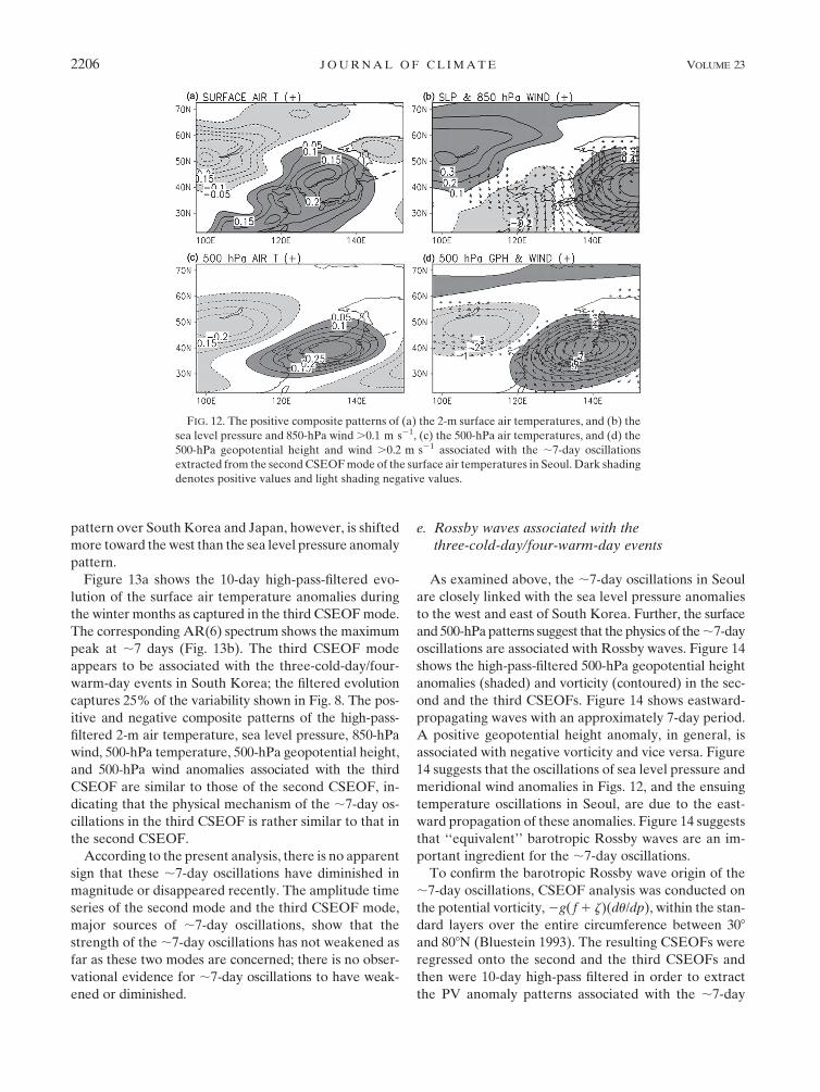
pattern over South Korea and Japan, however, is shifted
more toward the west than the sea level pressure anomaly
pattern.
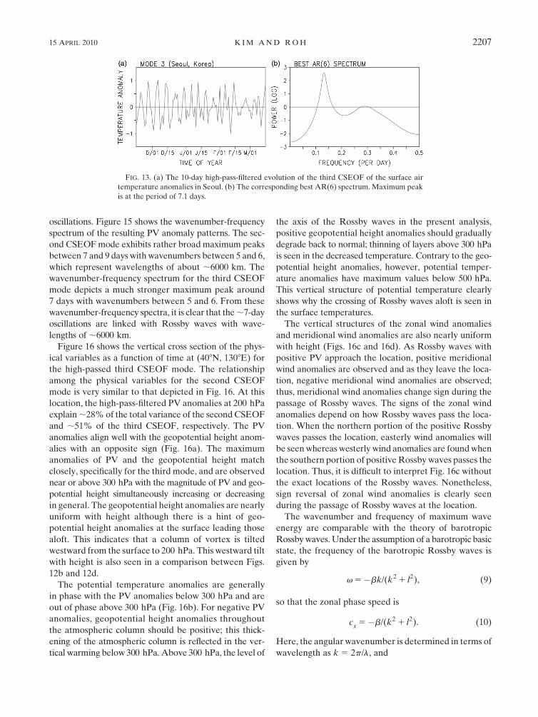
Figure 13a shows the 10-day high-pass-filtered evo-
lution of the surface air temperature anomalies during
the winter months as captured in the third CSEOF mode.
The corresponding AR(6) spectrum shows the maximum
peak at ;7 days (Fig. 13b). The third CSEOF mode
appears to be associated with the three-cold-day/four-
warm-day events in South Korea; the filtered evolution
captures 25% of the variability shown in Fig. 8. The pos-
itive and negative composite patterns of the high-pass-
filtered 2-m air temperature, sea level pressure, 850-hPa
wind, 500-hPa temperature, 500-hPa geopotential height,
and 500-hPa wind anomalies associated with the third
CSEOF are similar to those of the second CSEOF, in-
dicating that the physical mechanism of the ;7-day os-
cillations in the third CSEOF is rather similar to that in
the second CSEOF.
According to the present analysis, there is no apparent
sign that these ;7-day oscillations have diminished in
magnitude or disappeared recently. The amplitude time
series of the second mode and the third CSEOF mode,
major sources of ;7-day oscillations, show that the
strength of the ;7-day oscillations has not weakened as
far as these two modes are concerned; there is no obser-
vational evidence for ;7-day oscillations to have weak-
ened or diminished.
e. Rossby waves associated with thethree-cold-day/four-warm-day events
As examined above, the ;7-day oscillations in Seoul
are closely linked with the sea level pressure anomalies
to the west and east of South Korea. Further, the surface
and 500-hPa patterns suggest that the physics of the ;7-day
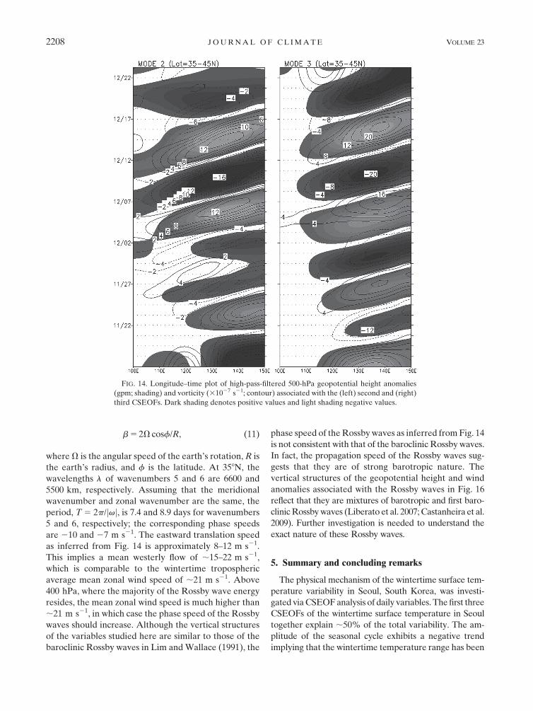
oscillations are associated with Rossby waves. Figure 14
shows the high-pass-filtered 500-hPa geopotential height
anomalies (shaded) and vorticity (contoured) in the sec-
ond and the third CSEOFs. Figure 14 shows eastward-
propagating waves with an approximately 7-day period.
A positive geopotential height anomaly, in general, is
associated with negative vorticity and vice versa. Figure
14 suggests that the oscillations of sea level pressure and
meridional wind anomalies in Figs. 12, and the ensuing
temperature oscillations in Seoul, are due to the east-
ward propagation of these anomalies. Figure 14 suggests
that ‘‘equivalent’’ barotropic Rossby waves are an im-
portant ingredient for the ;7-day oscillations.
To confirm the barotropic Rossby wave origin of the
;7-day oscillations, CSEOF analysis was conducted on
the potential vorticity, 2g( f 1 z)(du/dp), within the stan-
dard layers over the entire circumference between 308
and 808N (Bluestein 1993). The resulting CSEOFs were
regressed onto the second and the third CSEOFs and
then were 10-day high-pass filtered in order to extract
the PV anomaly patterns associated with the ;7-day
FIG. 12. The positive composite patterns of (a) the 2-m surface air temperatures, and (b) the
sea level pressure and 850-hPa wind .0.1 m s21, (c) the 500-hPa air temperatures, and (d) the
500-hPa geopotential height and wind .0.2 m s21 associated with the ;7-day oscillations
extracted from the second CSEOF mode of the surface air temperatures in Seoul. Dark shading
denotes positive values and light shading negative values.
2206 J O U R N A L O F C L I M A T E VOLUME 23
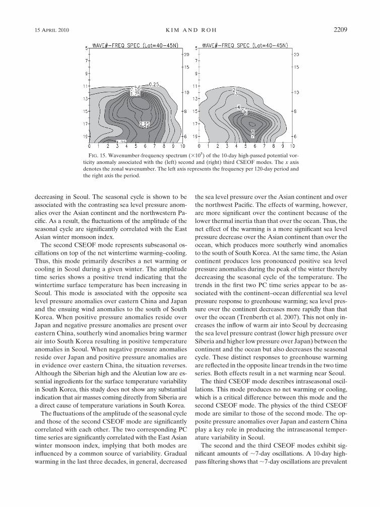
oscillations. Figure 15 shows the wavenumber-frequency
spectrum of the resulting PV anomaly patterns. The sec-
ond CSEOF mode exhibits rather broad maximum peaks
between 7 and 9 days with wavenumbers between 5 and 6,
which represent wavelengths of about ;6000 km. The
wavenumber-frequency spectrum for the third CSEOF
mode depicts a much stronger maximum peak around
7 days with wavenumbers between 5 and 6. From these
wavenumber-frequency spectra, it is clear that the ;7-day
oscillations are linked with Rossby waves with wave-
lengths of ;6000 km.
Figure 16 shows the vertical cross section of the phys-
ical variables as a function of time at (408N, 1308E) for
the high-passed third CSEOF mode. The relationship
among the physical variables for the second CSEOF
mode is very similar to that depicted in Fig. 16. At this
location, the high-pass-filtered PV anomalies at 200 hPa
explain ;28% of the total variance of the second CSEOF
and ;51% of the third CSEOF, respectively. The PV
anomalies align well with the geopotential height anom-
alies with an opposite sign (Fig. 16a). The maximum
anomalies of PV and the geopotential height match
closely, specifically for the third mode, and are observed
near or above 300 hPa with the magnitude of PV and geo-
potential height simultaneously increasing or decreasing
in general. The geopotential height anomalies are nearly
uniform with height although there is a hint of geo-
potential height anomalies at the surface leading those
aloft. This indicates that a column of vortex is tilted
westward from the surface to 200 hPa. This westward tilt
with height is also seen in a comparison between Figs.
12b and 12d.
The potential temperature anomalies are generally
in phase with the PV anomalies below 300 hPa and are
out of phase above 300 hPa (Fig. 16b). For negative PV
anomalies, geopotential height anomalies throughout
the atmospheric column should be positive; this thick-
ening of the atmospheric column is reflected in the ver-
tical warming below 300 hPa. Above 300 hPa, the level of
the axis of the Rossby waves in the present analysis,
positive geopotential height anomalies should gradually
degrade back to normal; thinning of layers above 300 hPa
is seen in the decreased temperature. Contrary to the geo-
potential height anomalies, however, potential temper-
ature anomalies have maximum values below 500 hPa.
This vertical structure of potential temperature clearly
shows why the crossing of Rossby waves aloft is seen in
the surface temperatures.
The vertical structures of the zonal wind anomalies
and meridional wind anomalies are also nearly uniform
with height (Figs. 16c and 16d). As Rossby waves with
positive PV approach the location, positive meridional
wind anomalies are observed and as they leave the loca-
tion, negative meridional wind anomalies are observed;
thus, meridional wind anomalies change sign during the
passage of Rossby waves. The signs of the zonal wind
anomalies depend on how Rossby waves pass the loca-
tion. When the northern portion of the positive Rossby
waves passes the location, easterly wind anomalies will
be seen whereas westerly wind anomalies are found when
the southern portion of positive Rossby waves passes the
location. Thus, it is difficult to interpret Fig. 16c without
the exact locations of the Rossby waves. Nonetheless,
sign reversal of zonal wind anomalies is clearly seen
during the passage of Rossby waves at the location.
The wavenumber and frequency of maximum wave
energy are comparable with the theory of barotropic
Rossby waves. Under the assumption of a barotropic basic
state, the frequency of the barotropic Rossby waves is
given by
v 5�bk/(k2 1 l2), (9)
so that the zonal phase speed is
cx
5�b/(k2 1 l2). (10)
Here, the angular wavenumber is determined in terms of
wavelength as k 5 2p/l, and
FIG. 13. (a) The 10-day high-pass-filtered evolution of the third CSEOF of the surface air
temperature anomalies in Seoul. (b) The corresponding best AR(6) spectrum. Maximum peak
is at the period of 7.1 days.
15 APRIL 2010 K I M A N D R O H 2207
b 5 2V cosf/R, (11)
where V is the angular speed of the earth’s rotation, R is
the earth’s radius, and f is the latitude. At 358N, the
wavelengths l of wavenumbers 5 and 6 are 6600 and
5500 km, respectively. Assuming that the meridional
wavenumber and zonal wavenumber are the same, the
period, T 5 2p/jvj, is 7.4 and 8.9 days for wavenumbers
5 and 6, respectively; the corresponding phase speeds
are 210 and 27 m s21. The eastward translation speed
as inferred from Fig. 14 is approximately 8–12 m s21.
This implies a mean westerly flow of ;15–22 m s21,
which is comparable to the wintertime tropospheric
average mean zonal wind speed of ;21 m s21. Above
400 hPa, where the majority of the Rossby wave energy
resides, the mean zonal wind speed is much higher than
;21 m s21, in which case the phase speed of the Rossby
waves should increase. Although the vertical structures
of the variables studied here are similar to those of the
baroclinic Rossby waves in Lim and Wallace (1991), the
phase speed of the Rossby waves as inferred from Fig. 14
is not consistent with that of the baroclinic Rossby waves.
In fact, the propagation speed of the Rossby waves sug-
gests that they are of strong barotropic nature. The
vertical structures of the geopotential height and wind
anomalies associated with the Rossby waves in Fig. 16
reflect that they are mixtures of barotropic and first baro-
clinic Rossby waves (Liberato et al. 2007; Castanheira et al.
2009). Further investigation is needed to understand the
exact nature of these Rossby waves.
5. Summary and concluding remarks
The physical mechanism of the wintertime surface tem-
perature variability in Seoul, South Korea, was investi-
gated via CSEOF analysis of daily variables. The first three
CSEOFs of the wintertime surface temperature in Seoul
together explain ;50% of the total variability. The am-
plitude of the seasonal cycle exhibits a negative trend
implying that the wintertime temperature range has been
FIG. 14. Longitude–time plot of high-pass-filtered 500-hPa geopotential height anomalies
(gpm; shading) and vorticity (31027 s21; contour) associated with the (left) second and (right)
third CSEOFs. Dark shading denotes positive values and light shading negative values.
2208 J O U R N A L O F C L I M A T E VOLUME 23
decreasing in Seoul. The seasonal cycle is shown to be
associated with the contrasting sea level pressure anom-
alies over the Asian continent and the northwestern Pa-
cific. As a result, the fluctuations of the amplitude of the
seasonal cycle are significantly correlated with the East
Asian winter monsoon index.
The second CSEOF mode represents subseasonal os-
cillations on top of the net wintertime warming–cooling.
Thus, this mode primarily describes a net warming or
cooling in Seoul during a given winter. The amplitude
time series shows a positive trend indicating that the
wintertime surface temperature has been increasing in
Seoul. This mode is associated with the opposite sea
level pressure anomalies over eastern China and Japan
and the ensuing wind anomalies to the south of South
Korea. When positive pressure anomalies reside over
Japan and negative pressure anomalies are present over
eastern China, southerly wind anomalies bring warmer
air into South Korea resulting in positive temperature
anomalies in Seoul. When negative pressure anomalies
reside over Japan and positive pressure anomalies are
in evidence over eastern China, the situation reverses.
Although the Siberian high and the Aleutian low are es-
sential ingredients for the surface temperature variability
in South Korea, this study does not show any substantial
indication that air masses coming directly from Siberia are
a direct cause of temperature variations in South Korea.
The fluctuations of the amplitude of the seasonal cycle
and those of the second CSEOF mode are significantly
correlated with each other. The two corresponding PC
time series are significantly correlated with the East Asian
winter monsoon index, implying that both modes are
influenced by a common source of variability. Gradual
warming in the last three decades, in general, decreased
the sea level pressure over the Asian continent and over
the northwest Pacific. The effects of warming, however,
are more significant over the continent because of the
lower thermal inertia than that over the ocean. Thus, the
net effect of the warming is a more significant sea level
pressure decrease over the Asian continent than over the
ocean, which produces more southerly wind anomalies
to the south of South Korea. At the same time, the Asian
continent produces less pronounced positive sea level
pressure anomalies during the peak of the winter thereby
decreasing the seasonal cycle of the temperature. The
trends in the first two PC time series appear to be as-
sociated with the continent–ocean differential sea level
pressure response to greenhouse warming; sea level pres-
sure over the continent decreases more rapidly than that
over the ocean (Trenberth et al. 2007). This not only in-
creases the inflow of warm air into Seoul by decreasing
the sea level pressure contrast (lower high pressure over
Siberia and higher low pressure over Japan) between the
continent and the ocean but also decreases the seasonal
cycle. These distinct responses to greenhouse warming
are reflected in the opposite linear trends in the two time
series. Both effects result in a net warming near Seoul.
The third CSEOF mode describes intraseasonal oscil-
lations. This mode produces no net warming or cooling,
which is a critical difference between this mode and the
second CSEOF mode. The physics of the third CSEOF
mode are similar to those of the second mode. The op-
posite pressure anomalies over Japan and eastern China
play a key role in producing the intraseasonal temper-
ature variability in Seoul.
The second and the third CSEOF modes exhibit sig-
nificant amounts of ;7-day oscillations. A 10-day high-
pass filtering shows that ;7-day oscillations are prevalent
FIG. 15. Wavenumber-frequency spectrum (3105) of the 10-day high-passed potential vor-
ticity anomaly associated with the (left) second and (right) third CSEOF modes. The x axis
denotes the zonal wavenumber. The left axis represents the frequency per 120-day period and
the right axis the period.
15 APRIL 2010 K I M A N D R O H 2209
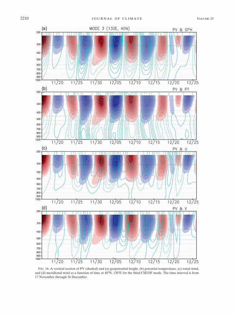
FIG. 16. A vertical section of PV (shaded) and (a) geopotential height, (b) potential temperature, (c) zonal wind,
and (d) meridional wind as a function of time at 408N, 1308E for the third CSEOF mode. The time interval is from
17 November through 26 December.
2210 J O U R N A L O F C L I M A T E VOLUME 23
over most of East Asia and the western North Pacific.
High-pass filtering of the wintertime surface tempera-
ture in Seoul, and the corresponding variability of the
physical variables, show that the ;7-day oscillations are
associated with opposite SLP anomalies to the east and
to the west of South Korea. These SLP anomalies pro-
duce surface wind anomalies to the south of South Korea.
Longitude–time plots of the sea level pressure anomalies
and zonal wind anomalies for these modes exhibit east-
ward propagation, indicating a Rossby wave origin of the
;7-day oscillations.
The eastward propagation of PV anomalies induces
changes in physical variables throughout the entire at-
mospheric column. Specifically, the passage of Rossby
waves is clearly seen in the surface temperature. The
wavenumber-frequency spectra of the PV anomalies for
the filtered second and the third CSEOFs show that
Rossby wave periods are 7–9 days for the second mode
and ;7 days for the third mode and the wavenumbers
are 5–6, equivalent to wavelengths of ;5500–6600 km at
358N. The ;7-day oscillations in Seoul are due to the
passing of Rossby waves, which induce the variability of
the same sign throughout the atmospheric column below
;300 hPa. In this sense, these Rossby waves may be
viewed as being of a nearly barotropic nature.
Rossby waves develop two opposite pressure anom-
alies: one to the west of South Korea and the other over
Japan. These opposite pressure anomalies develop sur-
face wind anomalies to the south of South Korea, which
is an essential ingredient for the ;7-day oscillations of
the surface temperature in Seoul. Rossby waves propa-
gate southeastward from Siberia and this propagation
induces changes in the entire atmospheric column; Rossby
waves do not directly supply warm–cold air into South
Korea from Siberia. It is the locations of the crests and
troughs of Rossby waves with respect to South Korea that
determine the surface temperatures in South Korea. Al-
though the opposite SLP anomalies are seen in both the
raw CSEOF modes and the high-pass-filtered modes,
their structures and natures are different from each other.
Whereas the continental SLP anomaly is stronger in the
raw CSEOF modes, the maritime SLP anomaly to the
east of South Korea is stronger in the high-pass-filtered
modes. The most striking difference is the clear eastward
propagation of SLP anomalies and other variables in the
high-pass-filtered modes; the raw CSEOF modes do
not exhibit eastward propagation clearly. In fact, when
high-pass-filtered anomalies were removed from the raw
CSEOF modes, the physical changes appear to be nearly
stagnant.
The ;7-day oscillations, also called the three-cold-
day/four-warm-day phenomenon in South Korea, are
associated with both the speed of the Rossby waves and
the speed of the mean zonal wind. The period of ;7-day
oscillations is determined by the eastward propagation
speed of the Rossby waves, which is the speed of the
mean zonal wind minus the phase speed of the westward
Rossby waves. The speed of eastward propagation should
also match with the period of the Rossby waves so that
alternating Rossby waves are periodically seen at the
same location. In this respect, this specific phenomenon
is an intricate interplay of Rossby waves and the mean
zonal wind. The asymmetry between cold days and warm
days is not clearly seen in the present study although
warm days tend to be slightly longer than cold days.
Acknowledgments. This work was funded by the Korea
Meteorological Administration’s Research and Develop-
ment Program under Grant CATER 2009-4211.
REFERENCES
Blackmon, M. L., J. M. Wallace, N.-C. Lau, and S. L. Mullen, 1977:
An observational study of the Northern Hemisphere winter-
time circulation. J. Atmos. Sci., 34, 1040–1053.
Bluestein, H. B., 1993: Observations and Theory of Weather Sys-
tems. Vol. 2, Synoptic–Dynamic Meteorology in Midlatitudes,
Oxford University Press, 594 pp.
Boyle, J. S., 1986: Comparison of the synoptic conditions in mid-
latitudes accompanying cold surges over eastern Asia for the
months of December 1974 and 1978. Part II: Relation of surge
events to features of the longer-term mean circulation. Mon.
Wea. Rev., 114, 919–930.
Castanheira, J. M., M. L. R. Liberato, L. De La Torre, H.-F. Graf,
and C. C. DaCamara, 2009: Baroclinic Rossby wave forcing
and barotropic Rossby wave response to stratospheric vortex
variability. J. Atmos. Sci., 66, 902–914.
Chang, C.-P., and K.-M. Lau, 1980: Northeasterly cold surges and
near-equatorial disturbances over the winter MONEX area
during December 1974. Part II: Planetary scale aspects. Mon.
Wea. Rev., 108, 298–312.
——, and ——, 1982: Short-term planetary-scale interaction over
the tropics and the midlatitudes during northern winter. Part I:
Contrast between active and inactive periods. Mon. Wea. Rev.,
110, 933–946.
——, J. E. Erickson, and K.-M. Lau, 1979: Northeasterly cold surges
and near-equatorial disturbances over the winter MONEX area
during December 1974. Part I: Synoptic aspects. Mon. Wea.
Rev., 107, 812–829.
Chang, J. C.-L., and L. Chongyin, 2004: The East Asia winter mon-
soon. East Asia Monsoon, C. P. Chang, Ed., World Scientific,
54–106.
Chu, P. S., and S.-U. Park, 1984: Regional circulation characteris-
tics associated with a cold surge event over East Asia during
winter MONEX. Mon. Wea. Rev., 112, 955–965.
Jhun, J.-G., and E.-J. Lee, 2004: A new East Asian winter monsoon
index and associated characteristics of the winter monsoon.
J. Climate, 17, 711–726.
Kalnay, E., and Coauthors, 1996: The NCEP/NCAR 40-Year Re-
analysis Project. Bull. Amer. Meteor. Soc., 77, 437–471.
Kang, I.-S., 1988: Recurrent tropospheric circulation anomalies in
the Northern Hemisphere associated with fluctuations of winter
monthly-mean temperature in Korea. J. Kor. Meteor. Soc., 24,
1–15.
15 APRIL 2010 K I M A N D R O H 2211
Kim, K.-Y., and G. R. North, 1997: EOFs of harmonizable cyclo-
stationary processes. J. Atmos. Sci., 54, 2416–2427.
——, ——, and J. Huang, 1996: EOFs of one-dimensional cyclo-
stationary time series: Computations, examples, and stochastic
modeling. J. Atmos. Sci., 53, 1007–1017.
——, K. Kullgren, G.-H. Lim, K.-O. Boo, and B.-M. Kim, 2006:
Physical mechanisms of the Australian summer monsoon. Part II:
Variability of strength, onset and termination times. J. Geophys.
Res., 111, D20105, doi:10.1029/2005JD006808.
Kullgren, K., and K.-Y. Kim, 2006: Physical mechanisms of the
Australian summer monsoon. Part 1: The seasonal cycle.
J. Geophys. Res., 111, D20104, doi:10.1029/2005JD006807.
Liberato, M. L. R., J. M. Castanheria, L. de la Torre, C. C. DaCamara,
and L. Gimeno, 2007: Wave energy associated with the variability
of the stratospheric polar vortex. J. Atmos. Sci., 64, 2683–2694.
Lim, G. H., and J. M. Wallace, 1991: Structure and evolution of
baroclinic waves as inferred from regression analysis. J. At-
mos. Sci., 48, 1718–1732.
Lim, Y.-K., and K.-Y. Kim, 2007: ENSO impact on the space–time
evolution of the regional Asian summer monsoons. J. Climate,
20, 2397–2415.
Newton, H. J., 1988: TIMESLAB: A Time Series Analysis Labo-
ratory. Wadsworth and Brooks/Cole, 623 pp.
Park, S.-W., and S.-S. Kim, 1987: The synoptic conditions in the
East Asian region accompanying cold-air outbreaks over Korea
during December 1985 through February 1986. J. Kor. Meteor.
Soc., 23, 56–90.
Ryoo, S.-B., J.-G. Jhun, W.-T. Kwon, and S.-K. Min, 2002: Cli-
matological aspects of warm and cold winters in South Korea.
Kor. J. Atmos. Sci., 5, 29–37.
——, W.-T. Kwon, and J.-G. Jhun, 2004: Characteristics of win-
tertime daily and extreme minimum temperature over South
Korea. Int. J. Climatol., 24, 145–160.
——, ——, and ——, 2005: Surface and upper-level features as-
sociated with wintertime cold surge outbreaks in South Korea.
Adv. Atmos. Sci., 22, 509–524.
Seo, K.-H., and K.-Y. Kim, 2003: Propagation and initiation
mechanisms of the Madden–Julian oscillation. J. Geophys. Res.,
108, 4384, doi:10.1029/2002JD002876.
Trenberth, K. E., and Coauthors, 2007: Observations: Atmospheric
surface and climate change. Climate Change 2007: The Phys-
ical Science Basis, S. Solomon et al., Eds., Cambridge Uni-
versity Press, 235–336.
Wallace, J. M., and M. L. Blackmon, 1983: Observation of low-
frequency atmospheric variability. Large-Scale Dynamical
Processes in the Atmosphere, B. J. Hoskins and R. P. Pearce,
Eds., Academic Press, 55–94.
Yang, S., K.-M. Lau, and K.-M. Kim, 2002: Variations of the east
Asian jet stream and Asian–Pacific–American winter climate
anomalies. J. Climate, 15, 306–325.
2212 J O U R N A L O F C L I M A T E VOLUME 23