Embed Size (px)
Citation preview

Physical phenomena of thinsurface layers
Katherine Ruth Thomas
Supervisor
Prof. Dr. Ullrich Steiner
A dissertation submitted for the degree of Doctor of Philosophy
July 2010
University of Cambridge
Cavendish Laboratory
Wolfson College


Declaration
This dissertation is the result of my own work and includes nothing which is the out-
come of work done in collaboration except where specifically indicated in the text. I
declare that no part of this work has been submitted for a degree or any other qualifi-
cation at this or any other university. This dissertation does not exceed the word limit
of 60,000 words set by the Physics and Chemistry Degree Committee.
Katherine R. Thomas. July 2010
i


AbstractPhysical phenomena of thin surface layers – Katherine R. Thomas
This thesis explores different physical phenomena observed in, or involving thin sur-
face films. Thin surface layers are ubiquitous. Found in nature and used in almost
every aspect of daily life, thin surface films are invaluable. While the applications and
roles may be varied, to be used effectively, the physical properties of these films and
the factors influencing their stability need to be well understood.
Surfaces can have a strong effect on the stability of thin films. In thin films of poly-
mer blends, wetting layers rich in one component often form at the film interface
prior to phase separation. Here the formation of these wetting layers are seen to
result in destabilisation of the film, even when the blend is far from phase coexis-
tence. A spinodal like instability with a characteristic wavelength is shown to form. A
theoretical model is developed, which describes the observed behaviour in terms of
coupled height and composition fluctuations in the wetting layer.
Spin coating is a common technique for the formation of thin polymer films. Films
formed in this way however, are often seen to exhibit anomalous properties, which
strongly differ from that of the bulk behaviour of the material. Here the rheological
properties and stored stresses in spin cast films are explored, with focus on the role
that the casting solvent plays in the properties of the film. The results suggest that the
observed deviation comes from a lowered density of chain entanglements. The effec-
tive viscosity and residual stresses in the as-spun film are seen to strongly depend on
the casting solvent properties and the solvent-polymer interactions.
The use of organometallic polymers as precursors for the formation of magnetic
ceramics is investigated. Emphasis is placed on doping the polymers with metallic
compounds prior to pyrolysis, allowing for the formation of technologically interest-
ing metallic alloys, without the need for new polymers to be synthesised. The for-
mation of iron-palladium alloys is demonstrated using this method. These are highly
desirable due to their potential use in hard-disk drive technologies.
Thin films can be used to influence the optical signature of a material and are
widely used in nature to produce vibrant, pure, iridescent colours. Here the optical
properties of the tropical plant Selaginella willdenowii are explored. The bright blue
colouration is seen to arise from a multilayer lamella structure on the upper surface
of the leaves. Light is important to plants, who use it both as an energy source and
an environmental signal. Blue iridescence occurs in a wide range of plant species,
suggesting that it has some adaptive benefit. These are considered and discussed.
iii


Acknowledgements
This thesis is a result of work carried out in the Thin Films and Interfaces at the
Cavendish Laboratory, University of Cambridge and was funded through a studentship
from the Engineering and Physical Sciences Research Council.
I would like to start by thanking my supervisor Prof. Ullrich Steiner, whose knowl-
edge, enthusiasm, advice and support guided me throughout my research. I would
particularly like to thank Ulli for allowing and encouraging me to take a three month
sabbatical to undertake a research project in industry. The opportunity was invalu-
able. Not all supervisors would have been so understanding or relaxed about my ab-
sence.
My thanks goes to all members of the Thin Films and Interfaces group past and
present for their help, friendship and support both in and out of the lab. To Alexis
Chennievre who worked with me for 3 months during his masters project on the
electrohydrodynamic instabilities, in particular on vapour annealing of the films. To
Rosa Poetes for all her help and advice with the ellipsometric measurements. To Na-
talyia Yufa and Silvia Vignolini who proofread large parts of this manuscript. To Maik
Scherer for solving all my LaTeX problems. And to Mathias Kolle who helped amongst
other things, with the optical measurements of the ferns.
Imaging in its different forms was an important part of the work carried out in this
thesis and could not have been achieved without the help of a number of people. I
would like to thank Chrissie Prichard and Jeremy Skepper for their help and advice on
embedding the ferns for TEM imaging. JJ Rickard for the many hours spent with me
trying every possible technique to get the best image possible of the ferns. Richard
Langford and Eric Tapley for your help with FIB milling.
I was fortunate to have enthusiastic, unstinting input from several external collab-
orators, without whom parts of the story told here would have been incomplete. Dr.
Nigel Clarke at the University of Durham, whose model was modified to explain the
behaviour seen in the polymer blends. Dr. Heather Whitney and Dr. Beverley Glover
at the department of Plant sciences for providing the biological perspective on the
role that iridescence might play in tropical ferns.
To my parents who have always been there for me. Thank you for your constant
support and encouragement in everything I have done; I would not have made it here
without it. To my sister and best friend Anne, for your unique perspective on life and
for keeping me sane. Hugs and waves. To Sam.
v


CONTENTS
1 Introduction 1
2 Theoretical Background 5
2.1 Polymer blends . . . . . . . . . . . . . . . . . . . . . . . . . . . . . . . . 6
2.1.1 Flory-Huggins theory . . . . . . . . . . . . . . . . . . . . . . . . . 6
2.2 Thin film stability . . . . . . . . . . . . . . . . . . . . . . . . . . . . . . . 10
2.2.1 Van der Waals forces and the Hamaker constant . . . . . . . . . 15
2.3 Stability of polymer blend thin films . . . . . . . . . . . . . . . . . . . . 16
2.4 Electrohydrodynamic instabilities . . . . . . . . . . . . . . . . . . . . . . 20
3 Wetting induced instabilities in miscible polymer blends 25
3.1 Materials and methods . . . . . . . . . . . . . . . . . . . . . . . . . . . . 28
3.2 Optical properties of the pure polymers . . . . . . . . . . . . . . . . . . 33
3.3 Results . . . . . . . . . . . . . . . . . . . . . . . . . . . . . . . . . . . . . 35
3.3.1 Surface enrichment . . . . . . . . . . . . . . . . . . . . . . . . . . 36
3.3.2 Surface instabilities . . . . . . . . . . . . . . . . . . . . . . . . . . 40
3.4 Conclusions . . . . . . . . . . . . . . . . . . . . . . . . . . . . . . . . . . 46
4 Out of equilibrium dynamics of thin polymer films 49
4.1 Materials and methods . . . . . . . . . . . . . . . . . . . . . . . . . . . . 56
4.1.1 Optical observation of instabilities . . . . . . . . . . . . . . . . . 61
4.2 Results and discussion . . . . . . . . . . . . . . . . . . . . . . . . . . . . 64
4.2.1 Toluene . . . . . . . . . . . . . . . . . . . . . . . . . . . . . . . . . 64
4.2.2 Trans-decalin . . . . . . . . . . . . . . . . . . . . . . . . . . . . . 70
4.2.3 Chloroform, MEK and THF . . . . . . . . . . . . . . . . . . . . . 77
4.2.4 Vapour annealing . . . . . . . . . . . . . . . . . . . . . . . . . . . 81
vii

4.3 Conclusions . . . . . . . . . . . . . . . . . . . . . . . . . . . . . . . . . . 84
5 Residual stress in thin polymer films 87
5.1 Materials and methods . . . . . . . . . . . . . . . . . . . . . . . . . . . . 89
5.2 Results and discussion . . . . . . . . . . . . . . . . . . . . . . . . . . . . 90
5.2.1 Cantilever bending . . . . . . . . . . . . . . . . . . . . . . . . . . 93
5.3 Conclusions . . . . . . . . . . . . . . . . . . . . . . . . . . . . . . . . . . 97
6 Palladium doped polymer precursors for magnetic ceramics 99
6.1 Materials and methods . . . . . . . . . . . . . . . . . . . . . . . . . . . . 102
6.2 Results . . . . . . . . . . . . . . . . . . . . . . . . . . . . . . . . . . . . . 107
6.3 Discussion . . . . . . . . . . . . . . . . . . . . . . . . . . . . . . . . . . . 116
6.4 Conclusions . . . . . . . . . . . . . . . . . . . . . . . . . . . . . . . . . . 120
7 Iridescence in tropical ferns 121
7.1 Introduction . . . . . . . . . . . . . . . . . . . . . . . . . . . . . . . . . . 124
7.2 Theoretical Background . . . . . . . . . . . . . . . . . . . . . . . . . . . 128
7.2.1 A single interface . . . . . . . . . . . . . . . . . . . . . . . . . . . 128
7.2.2 A single thin film on a substrate . . . . . . . . . . . . . . . . . . . 130
7.2.3 Multilayer reflections . . . . . . . . . . . . . . . . . . . . . . . . . 131
7.3 Materials and Methods . . . . . . . . . . . . . . . . . . . . . . . . . . . . 132
7.4 Results . . . . . . . . . . . . . . . . . . . . . . . . . . . . . . . . . . . . . 137
7.4.1 Modelling . . . . . . . . . . . . . . . . . . . . . . . . . . . . . . . 141
7.5 Discussion . . . . . . . . . . . . . . . . . . . . . . . . . . . . . . . . . . . 144
7.6 Possible adaptive advantages of iridescence . . . . . . . . . . . . . . . . 147
7.7 Conclusions . . . . . . . . . . . . . . . . . . . . . . . . . . . . . . . . . . 150
8 Conclusions 153
Bibliography 161
List of publications 183


CHAPTER
ONE
INTRODUCTION
This thesis is formed of a number of projects all with the common theme of surfaces
and thin films. The variety of projects is a result of three main factors. Firstly that I
chose to take an internship sabbatical half way through my PhD, secondly that I had
and took the opportunities to collaborate with a wide variety of different scientists
and finally that everything worked (well almost)!
Thin surface films or layers are ubiquitous. Found both in nature and in many tech-
nological applications, thin surface films have a wide variety of different roles. They
can influence the optical signature of a surface; a thin film with the right properties
coated onto the surface of a sheet of glass can act as an antireflective coating, reduc-
ing the glare from reflected sunlight. They can act as lubricants protecting objects
from wear, such as those found on the surface of our eyes which act to nourish and
protect the cornea. Another example is as memory devices where thin magnetic films
are used for data storage.
While the applications and roles may be varied, to be used effectively the physical
properties of these films need to be well understood. This thesis explores the physical
phenomena of a number of different thin films and can broadly be divided into three
1

Physical phenomena of thin surface layers
areas. The first looks at the stability of thin polymer films. The stability of a thin
film is important when considering its application, where a uniform homogenous
film is required, for example a layer of paint on the wall, it would be undesirable if
the film were to rupture and break-up. For a butterfly caught in the rain however, it
is important that a continuous film of water does not form on its wings, weighing it
down, but instead breaks up into droplets which will easily fall off.
Polymer blend films are often unstable, when taken from the one phase region to
the two phase region of phase space, due to phase separation of the different com-
ponents. In these films the surfaces can have a strong effect on the microstructure
evolution within the film during phase separation. Wetting layers rich in one compo-
nent are often seen to form at the film interfaces prior to phase separation [1] and can
lead to novel segregation within the film [2, 3]. These wetting layers are also seen to
form when the films are in the one phase region of phase space [4]. In chapter 3, the
formation of wetting layers at temperatures far from phase coexistence are seen to re-
sult in the spontaneous destabilisation of the film, causing a roughening of the poly-
mer/air interface. The blend is still in the one phase regime and no phase separation
is seen to occur. A spinodal like instability develops with a characteristic wavelength,
which is dependent on the composition of the blend. A theoretical description of
the destabilisation is developed, which explains the experimental results in terms of
the hydrodynamics of the film taking into account coupled height and concentration
variations within the wetting layer which forms.
Dewetting of a film is often undesirable. However, if the break up of a film can
be carefully controlled then the mechanisms causing this break up and the proper-
ties of the film can be probed. In thin polymer films, electric fields can be used to
drive destabilisation of the surface, resulting in the formation of a well defined pat-
tern [5]. The wavelength of this pattern is defined by the force balance acting on the
film, while the onset of the instabilities is dependent on the rheological properties
of the film. Experiments have shown that there is a discrepancy between the exper-
2

Introduction
imentally observed growth of these instabilities and that predicted theoretically [6].
It is thought that this may arise from non-equilibrium conformations of the poly-
mer chains and residual stresses in the film due to the preparation procedure [7].
In chapter 4 the effect of casting solvent on the properties of films formed by spin
coating is considered. The effective viscosity and the residual stresses of the as-spun
film are seen to be strongly dependent on the properties of the casting solvent and
the solvent-polymer interactions. The results show that the processing conditions of
the film are critical in determining the rheological properties and the conformation
of the polymer chains in the film. In chapter 5 the feasibility of using focused ion
beam milling to study the overall magnitude of the stresses in as-cast films polymer
films is investigated. This is done using a cantilever deflection technique, where the
cantilevers are milled into polymer films supported on silicon nitride membranes.
The initial experiments show that this technique is indeed feasible and indicate high
residual stresses in as-cast films.
The second phenomenon of thin films explored in this thesis is the use of poly-
mer films to form magnetic ceramics. Thin magnetic films are important in many
technological applications and can be used as sensors and for data storage. The use
of polymers as the precursors to the ceramics allows for the easy incorporation of
metallic nanoparticles into the films prior to ceramatisation and for the possible fab-
rication of complex and nanostructured shapes not possible with other film forma-
tion methods. A popular class of polymer to use as precursors are ferrocenes due to
the desirable magnetic properties of the resulting ceramics [8]. In chapter 6 one such
polymer polyferrocenylethylmethylsilane is doped with palladium prior to pyrolysis
and ceramic formation. The crystalline structure and the magnetic properties of the
resulting ceramics are investigated. Synthesis of new polymers can be an expensive
and time consuming process. Here instead palladium is mixed into the polymer, ei-
ther through the addition of nanoparticles or directly as acetyl acetonate, allowing
iron-palladium containing ceramics to be formed. Iron-palladium alloys are highly
3

Physical phenomena of thin surface layers
desirable due to their potential use in next generation hard-disk drives.
The final physical phenomena of thin films discussed in this thesis, is the use of
thin films to influence the optical signature of a material. Optically active structures
occur widely in nature and often result in the production of vibrant, pure, iridescent
colours [9]. Generally observed in insects and birds, optical structures are also seen
in plants but have not been as widely studied and as a result are poorly understood.
Plants use light both as an energy source for photosynthesis but also as an environ-
mental signal and are able to respond to its intensity, wavelength and direction. One
plant which displays iridescence is Selaginella willdenowii and is found growing in
the understorey of the Malaysian rainforests. The plant leaves are seen to display a
bright blue colouration. In chapter 7 the structures causing this colouration are in-
vestigated and the role that the iridescence might have to play in the plant discussed.
4

CHAPTER
TWO
THEORETICAL BACKGROUND
Polymers are long chain flexible molecules that consist of repeating molecular units
known as monomers. Due to the diversity of their properties both naturally occurring
and synthetic polymers are used in almost every aspect of modern day life. On the
molecular level polymers can be considered as chains, where the chain is not com-
pletely stretched but has a coil-like conformation. If the polymer is made up from a
single type of monomer then it is known as a homopolymer. Polymers can also be
formed from different monomers, with copolymers containing two chemically dif-
ferent monomers and terpolymers containing three. Polymers are formed during a
process known as polymerisation where each monomer is covalently bonded to the
next. The properties of the polymer depend on a number of parameters, including
the monomer used, the chain length, the distribution of the chain length (known as
the polydispersity) and purity. This chapter focuses on the theoretical description of
the stability of polymer blends and of thin polymer films.
5

Physical phenomena of thin surface layers
2.1 Polymer blends
Binary polymer blends are mixtures that consist of two chemically different polymer
species; polymer A and polymer B. The behaviour of a blend is determined by the
interactions between the two polymers. Entropic interactions always act to promote
mixing of the two components. Enthalpic interactions can however, act to promote
or inhibit mixing depending on the monomer-monomer interactions.
In polymer mixtures the entropy of mixing is very small due to the long chains of
the molecules involved. Miscibility of the polymers can therefore occur when the en-
thalpic interactions between the two polymers are favourable. Miscibility can also
occur when the enthalpic contribution is unfavourable, if it is smaller in magnitude
than the entropy of mixing. The monomer-monomer interactions are dependent on
a number of factors, including temperature and composition. As a result polymer
blends can exhibit both miscibility (homogeneous, one phase behaviour) and im-
miscibility (heterogeneous, two phase behaviour) depending on these parameters.
2.1.1 Flory-Huggins theory
A model for the thermodynamic compatibility of polymer blends was developed by
Flory [10] and Huggins [11] independently in the 1940’s. The Flory-Huggins lattice
model is a mean field theory that considers both the combinatorial entropy of mixing
and the enthalpic interactions between the monomers. The model assumes a mixture
of nA chains consisting of NA units of polymer A and nB chains consisting of NB units
of polymer B. The polymer chains are arranged randomly on a periodic lattice. Each
unit is assumed to be identical in size and occupies only one site.
The entropy of the system can be found by considering the total number of states
of the system and is determined using the Boltzmann relation S = k ln Ω, where Ω
is the number of ways the molecules can be arranged on the lattice. The resulting
6

Theoretical Background
expression for the entropy of mixing for a binary blend is given by
∆S mix = −kB
[φA
NAln φA +
φB
NBln φB
](2.1)
where φA,B is the fraction of sites occupied by monomers of polymer A or B and kB is
the Boltzmann constant. The 1/N factor arises from the fact that the monomers are
covalently bonded in groups of N, which cannot be independently dispersed. This
shows the strong influence of the chain length on the entropy of mixing and the mis-
cibility of polymer blends.
The enthalpic energy of the system depends on the monomer-monomer pair in-
teraction. In the model, this is assumed to come only from nearest-neighbour inter-
actions; identical and nonidentical monomer-monomer interactions. The enthalpy
of mixing is given by
∆H = kBTχφAφB (2.2)
where χ is the dimensionless Flory-Huggins interaction parameter. Flory and Hug-
gins considered χ to be purely energetic in origin varying as T−1. This implies that
for phase separation to occur the temperature of the blend must be lowered. How-
ever, phase separation is also seen to occur in some blends upon heating. Therefore χ
must also have an entropic contribution arising from packing constraints on the level
of polymer segments such that
χfh = A +BT
(2.3)
where A and B are constants, which vary from blend to blend. In classic Flory-Huggins
theory the interaction parameter is assumed to be independent of the volume frac-
tions of the two polymers. Experimentally however, it has been seen that the interac-
tion parameter can have a strong compositional dependence [12–14]. Here a compo-
7

Physical phenomena of thin surface layers
sition dependent interaction parameter is used with the form
χ(T, φ) =
(C1 −
C2
T
)(1 −C3φA) (2.4)
where C1, C2 and C3 are constants. The total free energy of the system Ffh can now be
written using equations 2.1 and 2.2
Ffh
kBT=φA
NAln φA +
φB
NBln φB + χ(T, φ)φAφB (2.5)
The entropic contribution to equation 2.5 is always negative, while the enthalpic con-
tribution can be either positive (opposes mixing) or negative (promotes mixing) de-
pending on the value of χ.
The Flory-Huggins free energy can be used to interpret the phase space of poly-
mer mixtures and to theoretically predict changes in the mixing behaviour such as
the coexistence or binodal curve. This is normally done using the common tangent
approach. The free energy vs. composition is plotted as a function of the tempera-
ture (see figure 2.1a). If the free energy is partially concave, a line can be drawn that
is tangent to Ffh and intercepts the curve in two places. These give the coexistence
compositions at that temperature. For a more detailed discussion see [15]. The bin-
odal curve defines the boundary between the one phase and two phase regions in
phase space and gives the equilibrium composition of the coexisting phases. The
temperature at which the phase boundary disappears defines the critical point. If
this extremum is a maximum then the system is said to have an upper critical solu-
tion temperature (UCST), while if it is a minimum then the system has a lower critical
solution temperature (LCST) (figure 2.1b).
The spinodal curve defines the limit of metastability; the region enclosed by the
spinodal is unstable while the region between the binodal and spinodal is metastable.
Equilibrium is reached slowly in polymer melts. For a blend heated to just inside the
8

Theoretical Background
Composition
Tem
pera
ture
Critical Point
Two Phase
Bino
dal
Spin
odal
One Phase
ΔF
/k(
K)
φA φB
Composition
a b
Figure 2.1: (a) Common tangent construction. (b) Example phase diagram for a lower criticalsolution blend.
two-phase region (between the spinodal and binodal curves), phase-separation oc-
curs via nucleation and growth; droplets of one phase form inside a matrix of another
slowly at discrete sites. If the temperature quench is deeper into the two phase region
(inside the spinodal region), then it becomes favourable for the system to phase sepa-
rate spontaneously; phase separation occurs uniformly throughout the material. The
spinodal defines the boundary between the two regimes of phase separation.
The binodal, spinodal and critical point can be found from equation 2.5 by con-
sidering the stability, equilibrium criteria and criticality.
• Binodal∆Ffh(φA) − ∆Ffh(φB)
φA − φB=
(∂∆Ffh
∂φ
)φA
=
(∂∆Ffh
∂φ
)φB
(2.6)
• Spinodal∂2∆Ffh
∂φ2 = 0 (2.7)
• Critical Point∂3∆Ffh
∂φ3 = 0 (2.8)
9

Physical phenomena of thin surface layers
2.2 Thin film stability
Thin liquid surfaces are never completely flat. Due to thermal motion of the molecules
a spectrum of capillary waves is always present. However, liquid films are in general
stable, since a sinusoidal perturbation of any given wavelength will result in an in-
crease in the surface area of the film and therefore an increase in the free energy of
the system. For the film to become unstable an additional “destabilising” force must
act at the surface of the film. This force can take on a number of different forms in-
cluding van der Waals forces (section 2.2.1), surface-tension forces, temperature gra-
dient effects [16, 17] and forces due to external fields such as an applied electrostatic
pressure (section 2.4). In this case the film can lower its free energy by changing its
thickness and is therefore unstable.
The stability of thin liquid films on solid substrates has been widely studied both
theoretically and experimentally [18–22]. The main stages of instability formation
and dewetting in thin films are generally well understood. The process of instabil-
ity formation can be modelled using a hydrodynamic approach where the thin liquid
film is approximated as an incompressible fluid. The motion of the fluid is then de-
scribed using the Navier-Stokes description of fluid flow with the appropriate bound-
ary conditions. The equations of motion are linearised by assuming that variations in
the height are small compared to their lateral extent (linear stability theory). The sta-
bility of the film is determined by whether these fluctuations grow or decay over time.
The resulting system of equations can be reduced to a simple description for the time
and spatial dependence of the height of the film, which can be used to determine the
conditions for instability formation. Pattern development and the dynamics of the
instabilities can be followed by studying these equations numerically.
This approach has been used to model a variety of systems such as the dewetting
of polymer films on solid substrates [21,22], the formation of instabilities in two-layer
liquid films [23] and the stability of films due to density variations [24]. Sharma et al.
10

Theoretical Background
h0
λ
z
xv(x)
Air
Polymer
Substrate
Figure 2.2: Schematic representation of capillary surface instabilities.
have shown that if the density of a film decreases with increasing film thickness, a
thermodynamically stable film can become unstable [24].
At temperatures above the glass transition temperature polymers can be described
as incompressible viscous fluids. Figure 2.2 shows a schematic representation of a
thin liquid film supported on a solid substrate. The local variation in height h(x, t) of
the polymer film at the polymer/air interface can be described by a one dimensional
sinusoidal function
h(x, t) = h0 + ξ exp(iqx + t/τ) (2.9)
where h0 is the average thickness of the film, ξ and q are the amplitude and wavevector
of the fluctuations respectively, t is the time and x the lateral coordinate parallel to the
surface. The time constant τ determines the temporal evolution of each fluctuation
with wavevector q. For positive values of τ the surface is destabilised by an amplifica-
tion of this mode, while negative values of τ correspond to damping. The wavelength
λ of the fluctuations is assumed to be large compared to the film thickness such that
λ = 2π/q h0 and the amplitude much smaller than h0.
The formation of a surface wave requires the lateral displacement of liquid within
the film. The velocity profile within the film can be determined using the Navier-
Stokes equation of motion for an incompressible Newtonian fluid.
ρ(∂tv + (v · ∇)v) = −∇p + η∇2v + ρg (2.10)
11

Physical phenomena of thin surface layers
This equation determines the liquid transport within the film, where v and η are the
velocity and viscosity of the liquid,∇p is the pressure gradient, which drives the liquid
flow in the film, g is the gravitational acceleration and ∂i is the partial derivative with
respect to i. The right hand-side of equation 2.10 gives the total force acting on a small
volume element moving in the fluid. This force stems from the pressure gradient,
viscous forces and gravity.
The polymer films considered in chapter 4 have very high viscosities, which re-
sults in a low fluid flow. As a result the convective term (v · ∇)v in equation 2.10 can be
neglected. The slow dynamic means that the velocity profile can always be consid-
ered to be in a quasi-steady state (∂tv = 0). Finally in thin films gravity is negligible.
Equation 2.10 can now be simplified to give
− ∇p + η∇2v = 0 (2.11)
The following assumptions are made about the thin liquid film. Firstly, a no-slip
boundary condition is assumed v(z = 0) = 0 at the film/substrate interface; there is
no liquid motion relative to the substrate. Secondly that normal stresses at the inter-
face are absent η∂zvliquid = 0. Taking these into account the velocity profile of the film
is
v(z) =12η
z(z − 2h)∂x p (2.12)
The averaged flux due to the lateral flow through a cross-section h of the film is given
by
j = hv =
∫ h
0v(z) dz =
h3
3η∂x p (2.13)
where v is the mean velocity. The continuity equation of the non-volatile liquid film
assuming incompressibility and taking into account mass-conservation is
∂th + ∂x j = 0 (2.14)
12

Theoretical Background
The equation of motion of the film/air interface can then be found by inserting equa-
tion 2.13 into equation 2.14.
∂th =13η∂x(h3∂x p) (2.15)
Here, p is the overall pressure acting at the surface of the liquid film. This is given by
p = p0 − γ∂xxh + pex(h) (2.16)
where p0 is the atmospheric pressure and γ is the surface tension. The second term
represents the Laplace pressure acting on the film, which stems from the curvature
of the interface. pex(h) is any excess surface pressure acting on the film.
Substituting the expression for the overall pressure acting at the surface into equa-
tion 2.15 along with equation 2.9, the dispersion relation for the system relating the
time constant τ to the wavevector q for a sinusoidal perturbation of the film can be
found using linear stability analysis [25].
1τ
= −h3
0
3η
[γq4 + ∂hq2
](2.17)
The dispersion relation can be used to determine whether a wave with wavevector q
is damped or amplified. This is shown in figure 2.3. In the absence of, or for a positive
excess pressure gradient (∂h pex ≥ 0) all growth rates are negative, the fluctuations will
be damped due to the restoring effect of surface tension. As discussed earlier, the film
will act to minimise its surface area, damping all perturbations. This is indicated by
the dashed line in figure 2.3. When ∂h pex < 0 (solid line in figure 2.3) long wavelength
fluctuations with 0 < q < qc =√−∂h pex/γ are amplified and the film will become
unstable, while short wavelength fluctuations are damped.
The fastest growing mode qmax is given by the maximum of equation 2.17,
q2max =
−12γ∂h pex (2.18)
13

Physical phenomena of thin surface layers
qc0
q
τ-1
Amplied
Damped
qmax
Figure 2.3: Graphical representation of the dispersion relation. In the absence of an appliedexternal field, all fluctuations are damped (dashed line). For a finite external pressure, fluctu-ations are amplified. The dispersion relation yields a dominant mode qmax with a correspond-ing growth rate τ−1
max.
the characteristic wavelength by:
λmax = 2π
√−2γ∂h pex
(2.19)
and the maximal growth rate by:
1τmax
=γh3
0
3ηq4
max (2.20)
This is proportional to the surface tension and inversely dependent on the viscosity
of the liquid.
Equations 2.19 and 2.20 together can be used to describe the static and dynamic
behaviour of the liquid film. The characteristic wavelength is a signature of the forces
acting on the liquid-air interface, while the time constant and growth rate can be used
to probe the rheological behaviour of the liquid film.
14

Theoretical Background
2.2.1 Van der Waals forces and the Hamaker constant
Van der Waals forces are an attractive or repulsive force, which acts between atoms or
molecules. They stem from polarisation effects between permanent and/or induced
dipoles. For two isolated atoms, the resulting force is proportional to the inverse sixth
power of the distance between the atoms [26]. This is known as the London equation.
Van der Waals forces exist not only between atoms and molecules but also between
particles and condensed media. These forces can be used to explain the dewetting
(break-up) of thin polymer films and wetting layers [27].
Consider a layer of thickness h sandwiched between two semi-infinite media. The
van der Waals forces between these media, give rise to an interaction free energy per
unit area of the form [28]
fvdW = −A
12πh2 (2.21)
where A is the effective Hamaker constant. The Hamaker constant determines the
interaction between the media and can be found using the Lifshitz theory [28]. The
Lifshitz theory is a continuum theory, which describes the van der Waals interactions
in terms of the dielectric properties of the media. The Hamaker constant for two
semi-infinite media 1 and 2, interacting across a layer 3, is approximated as
A ≈34
kT(ε1 − ε3
ε1 + ε3
) (ε2 − ε3
ε2 + ε3
)+
3hpve
8√
2
(n2
1 − n23
) (n2
2 − n23
)(n2
1 + n23
)1/2 (n2
2 + n23
)1/2(
n21 + n2
3
)1/2+
(n2
2 + n23
)1/2
(2.22)
where ε1, ε2 and ε3 are the dielectric permittivities and n1, n2 and n3 are the refractive
indices of the three media, hp is Plank’s constant and ve is the main electronic absorp-
tion frequency in the ultra-violet, which is typically around 3 × 10¹⁵ s−1. The first term
of equation 2.22 is the zero-frequency energy of the van der Waals interaction and the
second term is the dispersion energy contribution.
In thin films of polymer blends, surfaces can have a strong effect on the microstruc-
ture evolution within the film during phase separation. On quenching of the films
15
Physical phenomena of thin surface layers
from the one phase region to the two phase region of the phase diagram, wetting lay-
ers rich in one component of the polymer blend are often seen to form at the film
interfaces [1]. The formation of these layers can lead to novel segregation within the
films [2], with simultaneous phase separation and dewetting being observed [3]. In
chapter 3 equation 2.22 is used to calculate the Hamaker constant for a system where
media 1, 2 and 3 are the bulk polymer/polymer blend, air and a wetting layer rich in
poly(vinyl methyl ether) respectively. The first term in equation 2.22 is found to be on
the order of −4.5 × 10⁻²³ J. This is three orders of magnitude smaller than the second
term in equation 2.22, which is on the order of −1 × 10⁻²⁰ J. The first term is therefore
ignored.
When n1 > n3 > n2, as in chapter 3, the Hamaker constant is negative. This results
in a repulsive van der Waals force, which tends to increase the thickness of layer 3 in
order to lower the free energy. This repulsive or negative pressure in relation to van
der Waals forces is known as the disjoining pressure and can lead to a destabilisation
of the layer and the formation of instabilities due to the presence of an excess surface
pressure as shown earlier. The 1/h2 dependence of the van der Waals free energy svdW
(equation 2.21), signifies that the van der Waals forces are long-range forces and act
significantly over distances of up to 10 nm.
2.3 Stability of polymer blend thin films
In chapter 3, the formation of instabilities at the polymer/air interface in miscible
polymer blends is discussed. In such a system it is not enough to describe the sta-
bility only in terms of fluctuations in the height; composition fluctuations also play
an important role and must be considered. There have been many studies into the
behaviour of thin films of binary blends. However, all of these studies have been car-
ried out at the coexistence temperature or on films that are quenched deep into the
two phase region of the phase diagram where simultaneous phase separation and
16

Theoretical Background
dewetting are observed [3].
The mechanisms of instability formation and dewetting in thin films of polymer
blends, differ to that of single component films. In blends of deuterated oligomeric
styrene and oligomeric ethylene-propylene quenched into the two phase region, phase
separation is seen to induce dewetting of the films [29]. Holes are observed to form
first at the edges of the film and then move inwards. The rupture of the films oc-
curs on a faster time scale than that seen in single component films and has differ-
ent morphological characteristics. Evolving gradients in the concentration of the two
components at the surface of the film induce surface tension gradients, which pro-
vide an additional flow in the decomposition/dewetting front. It is thought that this
is responsible for the accelerated hole formation observed [30].
The formation of wetting layers in polymer blends, where one component prefer-
entially segregates to the polymer/air interface, prior to phase separation can induce
material heterogeneities and surface tension gradients in the films. These surface
tension gradients influence the hydrodynamics and mass transfer within the film and
are important when considering the destabilisation of these systems [30–32].
In a study by Clarke [33, 34], the stability of thin polymer blend films subject to
coupled height and composition fluctuations was investigated. He showed that such
a film will be less stable than one where either height or composition fluctuations
are considered in isolation. While this study focuses on films quenched in the two
phase region of the phase diagram, it was proposed that a thin film heated at temper-
atures corresponding to the bulk one-phase region may also become unstable when
these coupled fluctuations are considered. A modified version of this model is used in
chapter 3 to describe the instabilities observed. For completeness the original model
is explained here.
The model considers the coupling between surface-driven instabilities and com-
position instabilities in a thin film on a flat solid substrate with a free upper surface.
The following assumptions and conditions are applied. For simplicity fluctuations in
17

Physical phenomena of thin surface layers
composition are only allowed in the plane parallel to the substrate. For the model to
be physically realistic, the system of equations must conserve the total volume and
the relative amount of each component in the blend. The condition for fluctuations
in height and composition must correspond to the thermodynamic criteria based on
the free energy of the system. The model also assumes incompressibility; there is no
variation in the total density throughout the film. The total free energy of the film is
given by
FT =
∫ fb[φ(x)]h(x) + fs[φ(x), h(x)]
dx (2.23)
where x is the two-dimensional vector within the plane. fb[φ(x)] is the volume frac-
tion dependent free energy per unit volume within the film, which is independent of
height; since composition fluctuations are only allowed in the plane parallel to the
substrate, all unit volumes with coordinate x have the same composition. The total
local free energy in the bulk is therefore proportional to the height h(x) of the film with
respect to the substrate. fs[φ(x), h(x)] is the surface free energy per unit area, which is
dependent on the composition and the local height.
The model then considers the effect of perturbations in the composition φ(x) and
height h(x) about their average values φo and ho. The perturbations have the form
φ(x) = φo + δφ(x) (2.24)
h(x) = ho + δh(x) (2.25)
Substituting the above into equation 2.23, gives the total free energy to be
FT =
∫fb[φo + δφ(x)](ho + δh(x)) dx +
∫fs[φo + δφ(x), h0 + δh(x)] dx (2.26)
The bulk and surface free energies to the second order in the perturbations are
fb ≈ fb(φo) +∂ fb
∂φδφ(x) +
12∂2 fb
∂φ2 [δφ(x)]2 (2.27)
18

Theoretical Background
fs ≈ fs(φo, ho) +∂ fs
∂φδφ(x) +
12∂2 fs
∂φ2 [δφ(x)]2 +∂ fs
∂hδh(x) +
12∂2 fs
∂h2 [δh(x)]2 +∂2 fs
∂h∂φ[δh(x)][δφ(x)]
(2.28)
The conditions of volume and material conservation require that∫δh(x) dx = 0 and∫
(φo + δφ(x))(ho + δh(x)) dx = Bφoho, where B is the area of the film being considered.
These two conditions combine to give
∫δφ(x)δh(x) dx = −ho
∫δφ(x) dx (2.29)
the constraint for coupled height and composition fluctuations.
In order to determine the condition for instability formation, the free energy change
due to small sinusoidal spontaneous fluctuations of the form
δφ(x) = δφo + δφ1 sin(πx1
L
)sin
(πx2
L
)(2.30)
δh(x) = δh1 sin(πx1
L
)sin
(πx2
L
)(2.31)
are considered. B = 2L × 2L is the area of the film, where L is much greater than
the correlation length associated with gradients in the free energy. In a system where
height and composition fluctuations are not coupled, the condition for instability
formation is that the second derivative of the free energy with respect to height or
composition fluctuations is negative. This means that the free energy decreases due
to the fluctuations.
Considering equations 2.27, 2.28, 2.29 and 2.30, the total free energy has the form
FT = Fo − π2 f ′δφ1
δh1
ho+ π2 f ′′φ δφ
21
(1 +
δh21
4h2o
)+ π2 f ′′h δh
21 (2.32)
where
f ′ =
[∂ fs
∂φ− ho
∂2 fs
∂h∂φ
], f ′′φ =
12
(ho∂2 fb
∂φ2 +∂2 fs
∂φ2
), f ′′h =
12∂2 fs
∂h2 (2.33)
For the free energy to decrease with respect to a flat uniform film for some fluctuation
19

Physical phenomena of thin surface layers
δφ1 δh1, the curvature of the free energy must be somewhere negative.
The film is able to lower its total free energy by coupled height and composition
fluctuations if
f ′2 > 4h2o f ′′φ f ′′h (2.34)
This shows that even when both the second derivatives with respect to height and
concentration are positive the film may become spontaneously unstable, as long as
the surface free energy is concentration dependent. In this situation, coupled phase
separation and height variations are the only route to reduce the free energy.
Equation 2.34 gives the condition for instability formation in a thin film binary
mixture. The implications for stability when the mixture is miscible can now be con-
sidered. The model assumes that composition fluctuations only occur in two dimen-
sions; layers do not form parallel to the substrate. In many polymer blends however,
layering at the polymer/air interface is often seen due to surface enrichment by one
component. This surface segregation acts to lower the free energy of the film, which
according to this model can only serve to reduce the stability of the film. Equation
2.34 is then sufficient for the film to become unstable.
The model clearly shows that the coupling of height and composition fluctuations
is important when considering the stability of polymer blend films and provides a
starting point for modelling the dynamics of these systems.
2.4 Electrohydrodynamic instabilities
The formation of so-called electrohydrodynamic (EHD) instabilities, which develop
when a thin liquid film is sandwiched between two conductive media in a capaci-
tor like device, have been widely studied [6, 25, 35, 36]. Placing a liquefied insulator
in a plate capacitor geometry and applying an electric field perpendicular to the liq-
uid/air interface causes an amplification of low amplitude capillary surface waves,
20

Theoretical Background
U U U
a
b
h0
d
+ + + + + + + + +
- - - - - - - - -+ + + + + + + + +- - - - - - - - -
Figure 2.4: (a) Schematic representation of the capacitor setup used for the generation ofinstabilities in thin films by electric fields. The amplification of a surface instability is trig-gered by applying a voltage U. With time this instability grows causing the formation ofliquid columns which span the two plates. (b) Optical images of instabilities observed in apolystyrene film.
due to the presence of a destabilising surface excess pressure. EHD instabilities de-
velop with a characteristic wavelength λ. These instabilities then grow until fully form-
ed columns span the electrodes (figure 2.4). The physical mechanisms describing the
induced deformation of a liquid surface by an applied electric field, were first noted
by Swan in 1897 [37]. Since then many investigations have been carried out on this
type of system and the theory behind EHD instabilities is well understood [25, 38–40].
There are two main reasons behind the popularity in this approach for thin-film
destabilisation. The first, is as a method of pattern replication [6, 41–43]. When a
homogeneous force acts at the films surface, the resulting pattern will have a char-
acteristic wavelength, but will be laterally random. However, if a lateral variation in
the force field is introduced, for example by patterning the top electrode, the pattern
formation process can be guided to form a well defined structure (figure 2.5). Faithful
replication of the electrode pattern can be achieved with lateral dimensions down to
100 nm [5] and on timescales of a few seconds [36] depending on the properties of the
liquid film.
21

Physical phenomena of thin surface layers
B C D
2 μm
10 μm
20 μm20 μm 10 μm 20 μm
F G HE
A D
10 μm10 μm 10 μm10 μm
B C D
2 μm
10 μm
20 μm20 μm 10 μm 20 μm
F G HE
A D
10 μm10 μm 10 μm10 μm20
5 µ m
1 µ m
a c
b
Figure 1.15. Electrohydrodynamic pattern replication. (a): double-hexagonal pat-tern, (b): the word “nano”, (c): 140 nm wide and 140 nm high lines. In (b) theline width was ≈ 300 nm. The larger columns stem from a secondary (much slower)instability of the homogeneous (not structured) film. Adapted from [30] and [38].
Interestingly, the patterns generated by the applied electric field arenot stable in its absence. The change in morphology (from a flat film tostripes) significantly increases the polymer-air surface area. The verticalside walls of these line structures are, however, stabilized by the highelectric field (∼ 108 V/m). If the polymer is cooled below the glasstransition temperature before removing the electric field, as was donein our experiments, it is nevertheless possible to preserve the polymerpattern in the absence of an applied voltage.
Temperature Gradients. The same principle as in the case ofthe electric fields applies for an applied temperature gradient. Sincethe destabilizing pressure depends linearly on Jq (Eq. (1.21)), whichscales inversely with the plate spacing (Eq. (1.18)), there is also a strongdependence of the corresponding time constant with d. Therefore, thesame arguments as above apply here: the instability is generated firstat locations where d is smallest and the liquid material is drawn towardregions where the temperature gradient is maximal. This results in thereplication of a topographically patterned plate shown in Fig. 1.16 [39].This figure shows also that the pattern replication process is reasonablyrobust, with pattern sizes ranging from 5µm down to 1µm replicatedon the same sample. Figure 1.17 is another indication of the qualityof the replication process, showing that a master pattern was perfectlyreplicated over a 4 mm2 substrate area.
7.3. ELECTROSTATIC LITHOGRAPHY 99
0
50
100
0 1 2 3 4x(µm)
140 nm
Figure 7.4: The AFM image (top) shows 140 nm wide stripes (full width half maximum) in abrominated polystyrene film ( ≈ 45 nm) which replicate the silicon master electrode (200 nmstripes separated by 200 nm wide and 170 nm deep grooves). The device was annealed withan applied voltage of 42V at 170 C for 14 h. The cross-section on the bottom reveals astep height of 125 nm with an aspect ratio of ≈0.9.
pointed out. The quality of the replicated structures is nearly perfect. The elec-trostatically induced structure formation in the polymer film is not limited towavelengths around the intrinsic maximally amplified wavelength λ, but a largerange in lateral structures can be replicated for otherwise identical experimentalparameters. In the example of Fig. 7.4, lines with a width of 140 nm were repro-duced for an average plate spacing of 125 nm and an applied voltage of 42 V. Inthe AFM image, the resolution is limited by the geometry of the AFM tip. Therounded off corners at z = 0nm indicate a finite contact angle of the brominatedpolystyrene on the silicon oxide surface. Apart from this small effect, the profileof the polymer stripes is nearly rectangular with an aspect ratio (height/width)of ≈0.9. The high quality of the replication extends over the entire 100×100µm2
area which was covered by the master pattern.
Aspect ratios of up to 3 (900 nm high columns with a diameter of 300 nm) have
b c da
Figure 2.5: Electrohydrodynamic pattern replication using structured top electrodes.(a) Double-hexagonal pattern. (b) Lines are 140 nm wide and 140 nm high. (c) Circularcolumns. (d) Square columns. Scale bars (a) 5 µm, (b) 1 µm, (c) 20 µm, (d) 10 µm. Imagestaken from [25], [36] and [45].
The second use of this method of destabilisation is as a sensitive measurement
technique to quantitatively deduce the balance of forces at the liquid interface [44]
and the intrinsic physical properties of the liquid film. Barbero et al. [7] have shown
that by weakly perturbing the surface of a thin liquid film using an applied electric
field, the rheology and dynamics of the film can be probed. This will be discussed
further in chapter 4.
In the presence of an applied electric field equation 2.16 becomes
p = p0 − γ∂xxh + pdis(h) + pel(h) (2.35)
where pdis is the disjoining pressure, which results from intermolecular forces exerted
on the thin film. These include van der Waals interactions as discussed in section
2.2.1 and play a role in near surface regions. pel is the destabilising pressure, for an
applied voltage U, exerted on the interface by the interaction of the electric field with
the polarisation charges induced at the interface. If the liquid is a perfect dielectric in
a capacitor, the charges at the liquid/air interface experience an attractive interaction
with the charges on the upper electrode. The electrostatic pressure at the liquid/air
interface is given by
pel = −ε0εp(εp − 1)E2p = ε0εp(εp − 1)
U2
[εpd − (εp − 1)h]2 (2.36)
22

Theoretical Background
where ε0 is the permittivity of free space, εp is the dielectric constant of the liquid
polymer, d is the capacitor spacing and U is the applied voltage. Only the Laplace
term and the electrostatic pressure need to be taken into account due to the strong
electric fields generated in the system. The characteristic wavelength can be found
by substituting equation 2.36 into equation 2.19
λmax = 2π
√−2γ∂h pel
= 2π
√γU
ε0εp(εp − 1)2 E−3/2p = 2π
√γ[εpd − (εp − 1)h]3
ε0εp(εp − 1)2U2 (2.37)
and the characteristic onset time for instability formation is given by equation 2.20
τmax =η
γh30
(λmax
2π
)4
(2.38)
From these two equations it can be seen that the time dependence of instability for-
mation is strongly dependent on the thickness of the film and the pressure gradient.
It is also dependent on the viscosity of the liquid film and the surface tension.
23


CHAPTER
THREE
WETTING INDUCED INSTABILITIES IN MISCIBLE
POLYMER BLENDS
The composition of polymer blends at the surface and in the bulk often differs due
to the preferential adsorption of one component [1]. Driven by differences in surface
energies, the lower surface tension component is seen to segregate to the surface,
enriching the polymer/air interface [4, 46–48]. In miscible polymer blends this sur-
face enrichment is seen to be dependent on the molecular weights of the blend con-
stituents and the overall blend composition, with the width of the enriched wetting
layer being on the order of the correlation length ξ [49]. As the critical temperature
of the blend is approached ξ increases [50] and the width of the surface layer grows
rapidly [51].
Thin liquid films are easily deformed by material heterogeneities or thermal fluc-
tuations [52]. The interaction of the polymers with the free surface plays an impor-
tant role in the type of instability observed when thin films of polymer blends are
quenched from a homogeneous state to an unstable state in the two phase regime [53].
When one component is preferentially attracted to the polymer/air interface, surface-
directed spinodal decomposition waves evolve at this surface, propagating into the
25

Physical phenomena of thin surface layers
bulk, with wave vectors normal to the interface [54]. On quenching of the system, the
rapid formation of a surface enriched layer occurs prior to phase separation, induc-
ing material heterogeneities and surface tension gradients within the film. Surface
tension gradients have a strong influence on the hydrodynamics and mass transfer
within fluid systems [30–32], resulting in Marangoni-type flows within the film. The
liquid layer becomes unstable as a consequence of normal and lateral composition
gradients, giving rise to surface undulations.
Lateral surface modes can also evolve in the presence of neutral surfaces, which
do not have a preference for either polymer [30, 32, 55, 56]. These modes are similar
to those for energetically biased interfaces but have a much smaller amplitude than
spinodal decomposition waves, making them hard to resolve.
Blends of polystyrene (PS) and poly(vinyl methyl ether) (PVME) exhibit a lower
critical solution temperature (LCST) [57–60]. They offer an ideal system for the study
of the wetting behaviour of polymer blends due to their miscibility across all blend
compositions and strong segregation of PVME to the air surface. Investigations us-
ing two-dimensional nuclear magnetic resonance (NMR) suggest that this miscibility
results from a weak van der Waals interaction between the PS phenyl ring and the
PVME methoxy group, giving rise to a weakly negative interaction parameter [61, 62].
As the temperature of the blend is increased, this interaction is weakened and phase
separation of the blend occurs [63].
The miscibility of PS/PVME blends can be influenced by a number of parameters,
including the solvent in which the two polymers are initially mixed [64], the molecu-
lar weights of the polymers [65, 66], the film thickness [67]and through cross-linking
of the polymer chains [68]. For the majority of studies, PS/PVME blends are cast from
toluene solutions. Films produced in this way are homogeneous for all compositions
at room temperature. Trichlorethylene is also a common solvent for PS and PVME.
For films cast from trichloroethylene, the homogeneity of blends is seen to be de-
pendent on the volume fraction of the two polymer components [64]. Homogenous
26

Wetting induced instabilities in miscible polymer blends
films are observed at room temperature for φps < 0.25 and heterogenous films for
0.4 < φps < 0.97, where φps is the volume fraction of PS in the blend. Films with compo-
sition 0.25 < φps < 0.4 and φps > 0.97 have ‘slight’ heterogeneities. The homogeneous
films were found to have the same phase separation or cloud point temperature as
films cast from toluene.
In the one phase regime, PVME exhibits a strong surfactant behaviour and is seen
to wet the polymer-air interface [69, 70]. Bhatia et al. [4] showed, using X-ray photo-
electron spectroscopy (XPS) measurements, that a pure PVME wetting layer of 5−7 nm
thickness forms at the polymer/air interface. The surface enrichment of the PVME is
dependent on the molecular weights of the polymers and the overall blend composi-
tion.
Extensive work has been carried out on the phase separation of weakly miscible
polymer blends [67, 71–73]. Thin films of the blend were reported to undergo phase
separation induced by composition fluctuations [74]. Ogawa et al. studied the evo-
lution of 200 nm thick films heated at 115 C, which is in the two phase region for that
blend. They observed delayed dewetting of the films. During this incubation period,
the PVME was seen to segregate to the surface, while phase separation occurred in
the bulk. They suggest that the dewetting was induced by composition fluctuations
during the incubation period.
A further property of PS/PVME blends that has attracted a lot of attention is the
homogeneity of the blends at room temperature. Differential scanning calorimetry
(DSC) measurements have shown that PS/PVME blends exhibit a single glass transi-
tion temperature Tg, which is dependent on the composition of the blends [75]; this
is indicative of a homogeneous blend. However, other experiments carried out using
NMR spectroscopy and electron spin resonance oppose this view [76, 77]. They show
that on the scale of the polymer segments, for temperatures in the one phase region
but above Tg, the PS/PVME blends are not completely mixed. The blends are neither
strictly homogenous nor phase separated but instead microheterogeneous [75, 78, 79].
27

Physical phenomena of thin surface layers
This chapter focuses on previously unreported instabilities observed at the poly-
mer/air interface, which develop spontaneously in PS/PVME polymer blend thin films
in the one-phase regime, at temperatures well below their cloud point temperature.
Optical microscopy and atomic force microscopy were used to observed the surface
evolution of the films, while the changes in wetting behaviour were analysed using
ellipsometry.
3.1 Materials and methods
Polystyrene (PS) Mw = 100 kg mol−1, Mw/Mn = 1.04 and poly(vinyl methyl ether) (PVME)
50 wt.% H2O, were both obtained from Sigma-Aldrich. The PVME was dried in a vac-
uum oven at 60 C for 48 hrs and then placed under vacuum in a desiccator containing
phosphorous pentoxide (P2O5) for a further 24 hrs. Measurements of the PVME before
and after the dehydration process showed a mass loss of 50% confirming that all the
water had been removed. The molecular weight Mw = 78 kg mol−1 and polydispersity
Mw/Mn = 2.43 of the PVME were determined using gel permeation chromatography.
Solutions with various PS:PVME ratios in toluene were prepared and filtered through
a 0.1 µm PTFE filter.
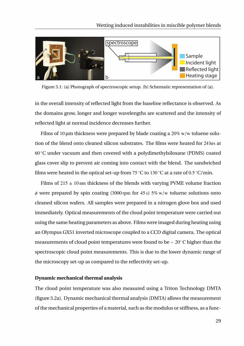
Cloud point measurements
Cloud point measurements were obtained by measuring the intensity of reflected
light at normal incidence as a function of temperature using an Ocean Optics USB
4000 spectroscope and DHL bal 2000 lightsource. The experimental setup is shown
in figure 3.1a. This technique was chosen due to the high resolution of the measure-
ments. As blends are heated and phase separation starts to occur, domains of one
phase start to form in a matrix of another phase. Once these domains become large
enough they start to scatter the low wavelength light of the incident lightsource. This
reduces the reflected intensity at normal incidence for this wavelength and a decrease
28
Wetting induced instabilities in miscible polymer blends
Incident lightReected light
Sample
Heating stage
spectroscope
a b
Figure 3.1: (a) Photograph of spectroscopic setup. (b) Schematic representation of (a).
in the overall intensity of reflected light from the baseline reflectance is observed. As
the domains grow, longer and longer wavelengths are scattered and the intensity of
reflected light at normal incidence decreases further.
Films of 10 µm thickness were prepared by blade coating a 20% w/w toluene solu-
tion of the blend onto cleaned silicon substrates. The films were heated for 24 hrs at
60 C under vacuum and then covered with a polydimethylsiloxane (PDMS) coated
glass cover slip to prevent air coming into contact with the blend. The sandwiched
films were heated in the optical set-up from 75 C to 130 C at a rate of 0.5 C/min.
Films of 215 ± 10 nm thickness of the blends with varying PVME volume fraction
φ were prepared by spin coating (3000 rpm for 45 s) 5% w/w toluene solutions onto
cleaned silicon wafers. All samples were prepared in a nitrogen glove box and used
immediately. Optical measurements of the cloud point temperature were carried out
using the same heating parameters as above. Films were imaged during heating using
an Olympus GX51 inverted microscope coupled to a CCD digital camera. The optical
measurements of cloud point temperatures were found to be ∼ 20 C higher than the
spectroscopic cloud point measurements. This is due to the lower dynamic range of
the microscopy set-up as compared to the reflectivity set-up.
Dynamic mechanical thermal analysis
The cloud point temperature was also measured using a Triton Technology DMTA
(figure 3.2a). Dynamic mechanical thermal analysis (DMTA) allows the measurement
of the mechanical properties of a material, such as the modulus or stiffness, as a func-
29

Physical phenomena of thin surface layers
Single CantileverBending
a b
Figure 3.2: (a) Photograph of Triton Technology DMTA. (b) Schematic representation andphotograph of the sample holder.
tion of the temperature. For these measurements, a specimen of known geometry is
subjected to a sinusoidal stress and the strain in the material is measured. This allows
the complex modulus of the material to be determined.
DMTA is a useful technique for characterising polymers as it can capture their vis-
coelastic behaviour. For purely elastic materials Hooke’s law applies i.e. the strain is
proportional to the applied stress. In this case the stress is independent of the strain
rate; the applied stress and the measured strain are in phase with one another. For
purely viscous or Newtonian materials, the stress is proportional to the strain rate.
For these materials, there is a 90 phase difference between the applied stress and
the measured strain. Viscoelastic materials such as polymers behave somewhere in
between and some phase difference will be measured.
DMTA measures the stiffness and damping, these are reported as the modulus and
tan δ. The modulus is expressed as the storage modulus (in-phase elastic component)
and the loss modulus (out of phase viscous component). The ratio of the loss modu-
lus to the storage modulus is known as tan δ and is a measure of the energy dissipation
of the material.
The DMTA was used to measure two properties of the polymer blends; the glass
transition temperature and the demixing temperature. The glass transition gives rise
30

Wetting induced instabilities in miscible polymer blends
-40 -20 0 200.02
0.04
0.06
0.08
0.10
0.12
Tan
δ
Temperature (oC)
2.0x10¹⁰
2.5x10¹⁰
3.0x10¹⁰
3.5x10¹⁰
4.0x10¹⁰
4.5x10¹⁰
5.0x10¹⁰
100 120 140 160
0.020
0.025
0.030
0.035
Tan
δ
Temperature (oC)
1.0x10¹⁰
1.2x10¹⁰
1.4x10¹⁰
1.6x10¹⁰
1.8x10¹⁰
2.0x10¹⁰
2.2x10¹⁰
Mod
ulus
(Pa)
a b
Temperature ( C)o
Figure 3.3: DMTA traces showing (a) cloud point temperature for φ = 0.3 (b) glass transitiontemperature for φ = 0.5.
to a large drop in the storage modulus and a peak in tan δ. The position of this peak
is dependent on the frequency of the applied stress. Phase separation is observed
by a change in the storage modulus and tan δ. The position of this peak is frequency
invariant [80].
Blend samples of 3− 5 mg of material were prepared in a glovebox and used imme-
diately. A heating rate of 1 C/min was used. The DMTA was used in single cantilever
bending mode with frequencies of 1 and 10 Hz. The size of the sample holder was
10 mm × 5 mm × 0.5 mm. This heating rate is greater than that used than for the other
two techniques due to limitations of the apparatus.
Figure 3.3 shows example traces for the DMTA measurements. All blends were seen
to exhibit a single glass transition temperature, which was dependent on the blend
composition (figure 3.3b). The demixing temperature of the blends was found to be
greater than the cloud-point temperatures measured using reflection spectroscopy
partly due to the higher heating rate and the lower resolution of the apparatus. Figure
3.3a shows an example temperature scan for a blend with φ = 0.3. 1 The demixing
temperature is indicated by the arrow.
1φ indicates the PVME content of the blend.
31

Physical phenomena of thin surface layers
CCD Camera
Analyser
MicroscopeObjective
Sample
Compensator
Polariser
Laser light source
a b
Figure 3.4: (a) Photograph of ellipsometer. (b) Schematic diagram of ellipsometer showingpositions of analyser, compensator and polariser.
Ellipsometry
To monitor surface evolution and wetting, films were first heated at T1 = 70 C (φ = 0.6, 0.7)
or T1 = 75 C (φ = 0.3, 0.4, 0.5) for 45 min, followed by heating at 10 C below the cloud
point temperature Tcp: T2 = Tcp − 10 C. Temperature measurements were accurate
to ±1 C. Wetting behaviour was monitored with an EP3 nulling imaging ellipsometer
(Nanofilm, Germany), while surface evolution was monitored using a Veeco Dimen-
sion 3100 atomic force microscope (AFM) (see section 4.1.1).
The thickness, refractive index and depth profile of the blend films were found us-
ing a model-dependent fit to the ellipsometry data. For these measurements, films
were prepared and annealed in a glove box. Ellipsometric measurements were then
carried out in air. Ellipsometry is a standard method for the determination of opti-
cal constants and thicknesses of polymer films on reflecting surfaces. It can also be
used to study more complicated systems and is able to resolve the interfaces between
polymer layers [81–83]. Unlike some other methods [84], ellipsometry allows for the
modelling of the composition across the entire thickness of the film.
Ellipsometry works by measuring the change in polarisation of light upon reflec-
tion from the interfaces of thin transparent films. A schematic diagram of the ellip-
someter can be seen in figure 3.4b. All nulling ellipsometers are based on six compo-
nents: a light source, a rotating polariser, a compensator, a sample, a rotating anal-
32

Wetting induced instabilities in miscible polymer blends
yser and a detector. The angles of the polariser, compensator and analyser at the
null condition are related to the ellipsometric quantities ∆ and Ψ, where tan (Ψ) is the
amplitude ratio of the parallel and perpendicular components of the polarised light
on reflection from the surface and ∆ is the phase difference. The optical properties
of the film cannot be deduced directly from ∆ and Ψ. Instead the optical properties
are found through comparison of the measured data with computational models of
∆model and Ψmodel allowing the properties of the film, for which the modelling data best
matches the experimental data, to be found.
Measurements with four zone accuracy were performed at a wavelength of 532 nm,
using a diode-pumped solid state laser, while varying the angle of incidence from 45
to 60. A 200 × 200 µm2 area was chosen as the region of interest for the measure-
ments. Care was taken to exclude local defects and dust. Each measurement lasted
about 45 min due to the time required for rotation of the polariser, analyser and com-
pensator between the four zones. Analysis was carried out for the film as spun, after
heating at T = T1 for 45 min and after heating at T2 = Tcp−10 C. Repeat measurements
showed no further changes.
The film thickness and surface roughness were measured using a Veeco Dimen-
sion 3100 atomic force microscope (AFM) in tapping mode. The use of atomic force
microscopy will be discussed in chapter 4.
3.2 Optical properties of the pure polymers
Reliable ellipsometric measurements require optical characterisation of the substrate
and the film materials. The bare silicon substrate was measured and modelled in
terms of the optical constants of bulk silicon, with a refractive index nSi(532 nm) =
4.15 and an extinction coefficient kSi = 0.01, covered by a native silicon oxide layer
with nSiOx = 1.5, kSiOx = 0 and dSiOx = 2 nm. These parameters were kept fixed for
all further measurements. Films of pure PVME and PS were spin-cast onto cleaned
33

Physical phenomena of thin surface layers
0.0 0.2 0.4 0.6 0.8 1.0
1.48
1.50
1.52
1.54
1.56
1.58
1.60
Linear Bruggerman Lorentz-Lorenz
Ref
ract
ive
Inde
x
φ(pvme)
Figure 3.5: Variation of refractive index with blend composition as predicted using the linear,Bruggerman and Lorentz-Lorenz effective medium models. The line is a guide for the eye.
silicon wafers and their thickness d and refractive index n were determined before
and after annealing at T1 for 45 min. For PS, n was seen to increase and d to decrease
slightly with annealing. The properties of the PVME film remained unchanged.
Since the initial measurements were performed directly after spin coating, the
changes in PS properties are likely to be caused by residual solvent in the film, result-
ing in a lower refractive index and a slightly swollen film. Upon heat treatment this
solvent is lost and the properties of pure PS are recovered. Additional heat treatment
resulted in no further changes in the refractive index or thickness of either film.
The refractive indices for the PS and PVME were found to be 1.61 and 1.47 respec-
tively (k = 0 for transparent polymers). This compares to 1.60 [85] and 1.467 [86] in
the literature. Based on these refractive indices, measured values of n for PS/PVME
blends were converted into PVME volume fractions φ by linear interpolation, which
closely approximates the Lorentz-Lorenz and Bruggeman effective medium approxi-
mations for refractive index (figure 3.5) [87–89].
34

Wetting induced instabilities in miscible polymer blends
5
60
70
80
90
100
110
120
1 0
140T
(°C
)
0.8 0.9
a
0.2 0.3 0.4 0.5 0.6 0.7 0.8 0.9
φb
0.2 0.3 0.4 0.5 0.6 0.7T (°C)
Inte
nsi
ty (
arb
. un
its)
b
140
70
80
90
100
110
120
130
50
60
70 12011010090800.95
1.00
1.05
1.30
1.25
1.20
1.15
1.10
Figure 3.6: (a) Coexistence curve for the PS/PVME blends. The circles are data from lightreflectivity experiments. The line is a fit using the common-tangent construction of the Flory-Huggins free energy. The triangles indicate the temperatures at which surface instabilitieswere observed. (b) Intensity of the reflected light as a function of temperature for φ = 0.6. Tcpis indicated by the arrow. The grey line is a guide for the eye.
3.3 Results
The cloud point curve for the bulk PS/PVME blend is shown in figure 3.6a. The cloud
point temperature Tcp, as measured by reflectivity, was taken to be the temperature at
which the intensity of reflected light first started to decrease from the baseline inten-
sity (figure 3.6b).
The experimental data were modelled by minimising the Flory-Huggins free en-
ergy
fb =φ
NAln φ +
1 − φNB
ln(1 − φ) + χφ(1 − φ) (3.1)
using the well established common-tangent technique (section 2.1.1), where NA and
NB are the degree of polymerisation of PVME and PS respectively. For this blend a
χ-parameter with a weak linear φ-dependence [14] is commonly used:
χ(T, φ) = (C1 −C2/T )(1 −C3φ) (3.2)
The parameters C1 = 0.0222, C2 = 7.32 K and C3 = 0.4 were determined by fitting the
35

Physical phenomena of thin surface layers
calculated binodal to the data in figure 3.6a. This yields the critical temperature for
the blend of Tc = 89 ± 1 C at a PVME volume fraction of φc = 0.63 ± 0.05.
The literature reports wide-ranging lower critical solution temperatures for blends
with molecular weight of PS and PVME similar to those used in this study [14, 57, 58, 90].
Nishi et al. [57] found Tc ∼ 100 C for Mw(PS) = 110 kg mol−1 and Mw(PVME) = 51.5 kg mol−1,
while Qian et al. found Tc ∼ 120 C for Mw(PS) = 100 kg mol−1 and Mw(PVME) = 75 kg mol−1
[14]. PVME is known to be highly hygroscopic and the presence of water can affect
the thermodynamics of phase separation. The lower value of Tc found here possibly
arises from the great care that was taken to ensure that the PVME and PVME con-
taining blends were water-free at all times. Repeat experiments showed highly repro-
ducible results for the determination of the coexistence curve.
3.3.1 Surface enrichment
Three individual ellipsometric measurements and surface roughness measurements
were carried out for five blend compositions. The temperature protocol was as fol-
lows: the films were measured as spun, after heating at T1 for 45 min and after heating
at T2 for 45 min. Figure 3.8 shows data for these three different measurements for a
film with φ = 0.6.
Each data set was initially fitted to three different models: a uniform film, a film
with a wetting layer and a film with a roughened wetting layer. These three models
are shown in figure 3.7. The fit to model C in figure 3.7 was comparable to that of
model B. AFM surface roughness measurements, showing a roughness of σ < 1 nm
for all films after these heating times, confirmed the absence of significant surface
roughness (figure 3.11a). Based on these observations, only model A and B were used
to analyse the data.
Initially the data are fitted well by assuming a film of uniform composition with
d = 224 nm and n = 1.538 (figure 3.8a). Heating the film at T1 for 45 min did not change
36

Wetting induced instabilities in miscible polymer blends
d
Air
Substrate
h0
db
Single Layer Double Layer Roughened Layer
A B C
Figure 3.7: Schematic diagram of the models used to fit the ellipsometric data. (a) Uniformfilm (single layer). (b) PVME enriched surface layer (two layer model). (c) Roughened PVMEsurface layer (three layer model).
the fitted d and n values, indicating the absence of residual solvent in the PVME rich
film. The fitted values from the two layer model converge to a single layer model with
n = nb = ns where nb is the refractive index of the bulk layer and ns is the refractive
index of the surface layer and did not improve the quality of the fit.
The film was then heated at T2 = 80 C for 45 min. The ellipsometric angles of the
data in figure 3.8c are no longer well described by a single layer fit. Instead, a dou-
ble layer model with db = 208 nm, nb = 1.529, h0 = 19 nm and ns = 1.482 provides
a much better fit to the data. An AFM topography image of the surface showed no
sign of surface roughness, indicating that the resulting changes must be due to a wet-
ting layer, not to a roughening of the polymer/air interface (figure 3.11a). The lower
refractive index of the wetting layer indicated an increased PVME content at the sur-
face as compared to the bulk. A detailed analysis of the fit parameters was consistent
with material conservation with respect to the initial uniform film.
Similar measurements were carried out for all the blend compositions indicated
in figure 3.6a and the trend in sample composition with temperature was confirmed.
As-cast and films annealed at T = T1 could be fitted by a single layer model, while
films heated at T = T2 for 45 min were all best described by a two layer model with a
PVME enrichment layer of h0 = 21 ± 3 nm and a reduced refractive index as compared
to the bulk.
The thickness of the PVME surface enrichment layer can be compared to the bulk
correlation length of PS/PVME blend for T − T2. The correlation length is both com-
37

Physical phenomena of thin surface layers
Psi
a b c
Figure 3.8: Variation of the ellipsometric angles Delta () and Psi () with the angle of inci-dence for a sample with φ = 0.6. The lines are fits to the data for a uniform film composition(black lines) and a film with a PVME-rich surface layer (grey lines). (a) Film as spun. Sin-gle layer fit: d = 224 ± 7 nm, n = 1.538. Double-layer fit: db = 207 ± 8 nm, nb = 1.528 andh0 = 20 ± 10 nm, ns = 1.515. (b) Film heated at 70 C for 45 min. Single layer fit: d = 224 ± 7 nm,n = 1.535. Double layer fit: db = 207 ± 7 nm, nb = 1.535 and h0 = 22 ± 3 nm, ns = 1.538.(c) Film heated at 80 C for 45 min. Single layer fit: d = 228 ± 8 nm, n = 1.517. Double layer fit:db = 208 ± 8 nm, nb = 1.529 and h0 = 19 ± 2 nm, ns = 1.482.
position and temperature dependent [91].
ξ =a6
/√1 − φb
2NA+
φb
2NB− χ(T, φ)φb(1 − φb) (3.3)
where a is the statistical segment length [92] and φb is the bulk composition suffi-
ciently far from the surface. The correlation length varies from 19± 2 nm for φ = 0.3 to
20± 2 nm for φ = 0.4− 0.6 and 18± 2 nm for φ = 0.7. Within the error margins, the fitted
width of the PVME enrichment layer is identical to the bulk correlation length of the
blend, in agreement with mean field theories.
Figure 3.9a shows the variation of the normalised surface excess as a function of φb
z∗ =a6
∫ φb
φs
dφ
√(1 − φ)
fb(φ) − fb(φb) − (φ − φb)∆µ(3.4)
where φs is the surface composition and ∆µ is the chemical potential difference be-
tween blends with φb and φs [93]. The insets show the composition profile for φ = 0.3
38

Wetting induced instabilities in miscible polymer blends
0 20 40 60 80 1000.1
0.2
0.3
0.4
0.5
0.6
0.7
0.8
0.9
1.0
φ
z (nm)
0 20 40 60 80 1000.1
0.2
0.3
0.4
0.5
0.6
0.7
0.8
0.9
1.0
φ
z (nm)
0.3 0.4 0.5 0.6 0.70.0
0.5
1.0
1.5
2.0
2.5
3.0
z* (x
10-9
)
φb
φb
a b
c
Figure 3.9: (a) Variation of the surface excess with φ after annealing for 45 min atT2 = Tcp − 10 C. Composition profile of blends with overall blend composition (b) φ = 0.3and (c) φ = 0.5. All surface layers have the same thickness of h0 = 21 ± 3 nm. The solid lineshows the ellipsometric model and the broken line prediction of equation 3.5.
(figure 3.9b) and φ = 0.5 (figure 3.9c). The squares show the experimental surface ex-
cess based on the ellipsometric step model fit to the wetting layer (solid line in figure
3.9b, c). The ellipsometric model is however only the most simple approximation for
the surface enriched layers. Mean field models predict an exponential variation of
the composition at the surface
φ(z) = φb + (φs − φb) exp(−z/ξ) (3.5)
The predictions of equation 3.5 are shown in figure 3.9 (broken lines) alongside the
step profiles (solid lines). Both models have the same values of z∗.
To improve the ellipsometric model, a series of step functions can be used to bet-
ter approximate the predicted exponential variation of z∗. Adding a third layer to the
model resulted in fits with a top layer of φ ' 1. This is in agreement with published
values for the PVME surface enrichment of 98% [4, 69] and leaves z∗, h0 and φb es-
sentially unchanged. Since this more complex layer sequence did not significantly
improve the fit in figure 3.8c, data analysis was confined to the model with the fewest
fit parameters that adequately describes the data (i.e. the simple two-layer box model
shown in figure 3.7b).
39

Physical phenomena of thin surface layers
a b
0nm
100nm
0nm
15nm
0
15o
o
0o
5o
0nm0 10 20 30 40 50-3.0
-1.5
0.0
1.5
3.0
Hei
ght (
nm)
µm
0 10 20 30 40 50
-25-20-15-10
-505
1015
Hei
ght (
nm)
µm
d e
c
f
Figure 3.10: AFM micrographs of a (a,b) 210 nm thick film with φ = 0.4 heated at 95 C for180 min. The AFM topography image in (a) shows the formation of capillary surface instabil-ities with a wavelength ∼ 4 µm and an amplitude of (c) ∼ 1 nm. (d,e) AFM micrographs of a210 nm thick film with φ = 0.6 heated at Tcp for 180 min. Lateral phase separation is seen inboth the height and phase images. (f) Roughness of cross-section of (d).
3.3.2 Surface instabilities
The surface topography of a 210 nm film with φ = 0.4, heated at T2 = 95 C is shown in
figure 3.10a. Initially, the surface stayed planar. However, after extended annealing,
the formation and growth of surface instabilities was observed. The AFM topography
images of the film in figure 3.10a reveal a spinodal-like pattern with a characteristic
wavelength λ, which varies as a function of blend composition (figure 3.12). The lack
of contrast in the AFM phase images in figure 3.10b confirms the absence of a lat-
eral composition variation. The contrast in figure 3.10a therefore arises solely from
a variation in surface topography. The optical micrograph in figure 3.11b confirms
the initial smoothness of the film, while figure 3.11c shows additional structure on a
larger length scale for the film of figure 3.10a. Similar roughening is seen for all blend
compositions.
40

Wetting induced instabilities in miscible polymer blends
c
0mins 180mins0nm
15nm
a b
Figure 3.11: (a) AFM topography image of a sample after heating at T2 for 45 min. (b, c) Opti-cal micrographs of a 210 nm film with φ = 0.4 heated at 95 C. The optical micrograph of theunannealed film in (a) confirms the smoothness of the initial film, while the optical contrastof the film annealed for 180 min in (c) possibly indicates the onset of dewetting by nucleation.Scale bar is 100 µm.
Figures 3.10d,e show the AFM images for a film with φ = 0.6 heated at Tcp for 3 hrs.
Phase separated domains are observed in both the height and phase images. The
topology is very different to that seen in figure 3.10a and the roughness is increased
by one order of magnitude (figure 3.10c, f). This confirms that the instabilities ob-
served in figure 3.10a do not arise from lateral composition variations due to phase
separation of the polymers.
The spontaneous formation of capillary instabilities in a non-critical polymer blend
is surprising due to the lack of any apparent surface pressure driving the instability.
While there is considerable literature on the pattern formation in unstable binary
blends, these predominately arise from a lateral variation of surface composition,
which is clearly not the case here. Very recently, Thiele and coworkers [30] performed
model calculations testing the stability of complete wetting layers that coexist with a
bulk of coexisting composition (i.e. bulk compositions that lie on the binodal line).
The films in these experiments, while close to bulk coexistence, are clearly in the one-
phase regime of the phase diagram.
Clarke [33] has shown that a thin layer of a binary mixture may become unstable
with respect to coupled height h and composition φ fluctuations, even if the layer is
41

Physical phenomena of thin surface layers
0.3 0.4 0.5 0.6 0.7
2
4
6
8
10
12
λ (μ
m)
φb
Figure 3.12: () Experimentally determined wavelength of the instability as a function of theblend composition, measured after 3 hrs of heating at T2. (•) Theoretically determined wave-length found using experimental parameters. The lines are a guide for the eye.
stable to both height and composition fluctuations when treated independently. The
condition for instability formation is given by
[∂ fs
∂φ− h0
∂2 fs
∂h∂φ
]2
> h20
(h0∂2 fb
∂φ2 +∂2 fs
∂φ2
)∂2 fs
∂h2 (3.6)
where h0 is the initial height of the unperturbed layer and fb is the composition de-
pendent local free energy per unit volume within the layer, which is assumed to be
independent of h. The model assumes that all unit volumes with the same coordi-
nate in the plane of the layer have the same composition. Hence the total local free
energy density due to the bulk is proportional to the height of the film with respect to
the substrate. The local surface free energy per unit area fs is both h and φ dependent.
As shown in [34], the dynamics of an instability in the plane of the film are described
by the two dimensional equations of motion
h∂φ
∂t= −∇ · [hM∇µKφ] +
φh3
3η(∇µKφ)(∇φ) (3.7)
and∂h∂t
= −13η∇ · h3∇µKh (3.8)
42

Wetting induced instabilities in miscible polymer blends
The first term on the right hand side of equation (3.7) represents the diffusive flux,
driven by gradients in the chemical potential difference between the two compo-
nents µKφ = δFT/δKφ, where FT is the total free energy and M is the mobility of the
blend. The second term represents the coupling to hydrodynamics and depends on
the blend viscosity η. Equation (3.8) describes the hydrodynamic flow in thin films,
which is driven by gradients in the disjoining pressure µKh = δFT/δKh. The subscript K
in the chemical potential and the disjoining pressure denotes constrained functional
derivatives [94, 95]. These ensure that the functional form of the disjoining pressure
and the chemical potential take into account the constraints of material and compo-
sition conservation. Linearisation of equations (3.7) and (3.8) to first order in height
and composition fluctuations leads to
(3η/h30)∂δh/∂t
(1/M)∂δφ/∂t
= A
δhδφ . (3.9)
If it is assumed that composition and height gradients can be accounted for within
the free energy by the contributions κ(∇φ)2 and σ(∇h)2 respectively, where κ is the in-
terfacial energy and σ is the surface tension, then the components of the matrix are
given by
A11 = −q2(∂2 fs
∂h2 + 2q2σ
)A12 = A21 = q2 1
h0
(∂ fs
∂φ− h0
∂2 fs
∂h∂φ
)(3.10)
A22 = −q2(h0∂2 fb
∂φ2 +∂2 fs
∂φ2 + 2h0κq2)
The solution to equation (3.9) is
δφ = c11eR1t + c12eR2t
δh = c21eR1t + c22eR2t (3.11)
43

Physical phenomena of thin surface layers
where the constants ci j are determined by the statistical correlations of the functions
prior to the layer becoming unstable. The two rates are the solution to
∣∣∣∣∣∣∣∣∣h3
03ηA11 − R h3
03ηA12
MA12 MA22 − R
∣∣∣∣∣∣∣∣∣ = 0. (3.12)
Whilst the q-dependence of the rates depends on both the viscosity and mobility, the
critical wave vector, the wavelength below which fluctuations are unstable and grow
can be determined, without knowledge of either of these parameters. If A11, A22 > 0
then one of the solutions to equation (3.12) is equal to zero when
A11A22 − A212 = 0. (3.13)
To make further progress, it is necessary to choose a functional form for the bulk and
surface energies. The bulk free energy is determined using the Flory-Huggins theory,
such that∂2 fb
∂φ2 =2kBT (χs − χ)
a3 (3.14)
where χs is the value of the interaction parameter on the spinodal curve. The factor
kBT/a3 ensures that the energy scales of the bulk and surface energies are matched
appropriately. The surface free energy is given by fs = −AH/πh2, where AH is the com-
position dependent Hamaker constant. It is found using the Lifshitz theory [28] and
is given by
AH = d1(d2(φb − φs)) − d3φbφs (3.15)
where d1 = 3.867 · 10−22 J, d2 = 54.328 and d3 = 10.452 are constants calculated using
the refractive indices of the bulk and surface layers with compositions φb and φs.
The interfacial energy is given by [96]
κ =kBTa3
(a2
36φ(1 − φ)
)(3.16)
44

Wetting induced instabilities in miscible polymer blends
For the surface energy a fixed value of σ = 30 mNm−1 [85] was used.
One difficulty that arises from assuming discrete wetting is that the composition
of the surface layer falls inside the bulk two-phase region for some compositions
and hence should be unstable. However, this interpretation is based on the bulk
behaviour and it is known that for thin layers the transition temperature is shifted
upwards for LCST behaviour [97]. In order to overcome this difficulty, the value of the
interaction parameter required for an instability to form is considered and given such
values, the resulting critical wave vector of the instability is determined.
Unstable fluctuations are found for 0 < (χs−χ) < 1.5 ·10−5. It should be emphasised
that for these conditions both ∂2 fb/∂φ2 and ∂2 fs/∂h2 are positive, so that when consid-
ered independently the layer is stable to either concentration or height fluctuations;
it is the coupling between the two that leads to the instability.
The theoretical values of the critical wavelength, λc = 2π/qc, found using the ex-
perimentally determined φb and φs for (χs − χ) = 1.4 × 10⁻⁴ are shown in figure 3.12.
The critical wavevector qc is given by the solution to equation 3.13, which is quadratic
in q2c
4h0κσq4c +2
[σ
(h0∂2 fb
∂φ2 +∂2 fs
∂φ2
)+ h0κ
∂2 fs
∂h2
]q2
c +
(h0∂2 fb
∂φ2 +∂2 fs
∂φ2
)∂2 fs
∂h2 −1h2
0
(∂ fs
∂φ− h0
∂2 fs
∂h∂φ
)2
= 0
(3.17)
The trend is qualitatively similar to that seen in the experimental data, with the abso-
lute values of the critical wavelength being comparable to the fastest growing wave-
length. For both phase separation and dewetting, the relation between the critical
and the fastest growing wavelength is given by qm =√
2qc. Although such a simple
relation does not exist for the coupled process, it seems reasonable to assume that
the trend associated with the critical wavelength is a good indication of that expected
for the fastest growing wavelength.
The compositional dependence shown in figure 3.12 arises from the dependence
of the Hamaker constant AH on both φs and φb, as seen in equation 3.15. The driving
45
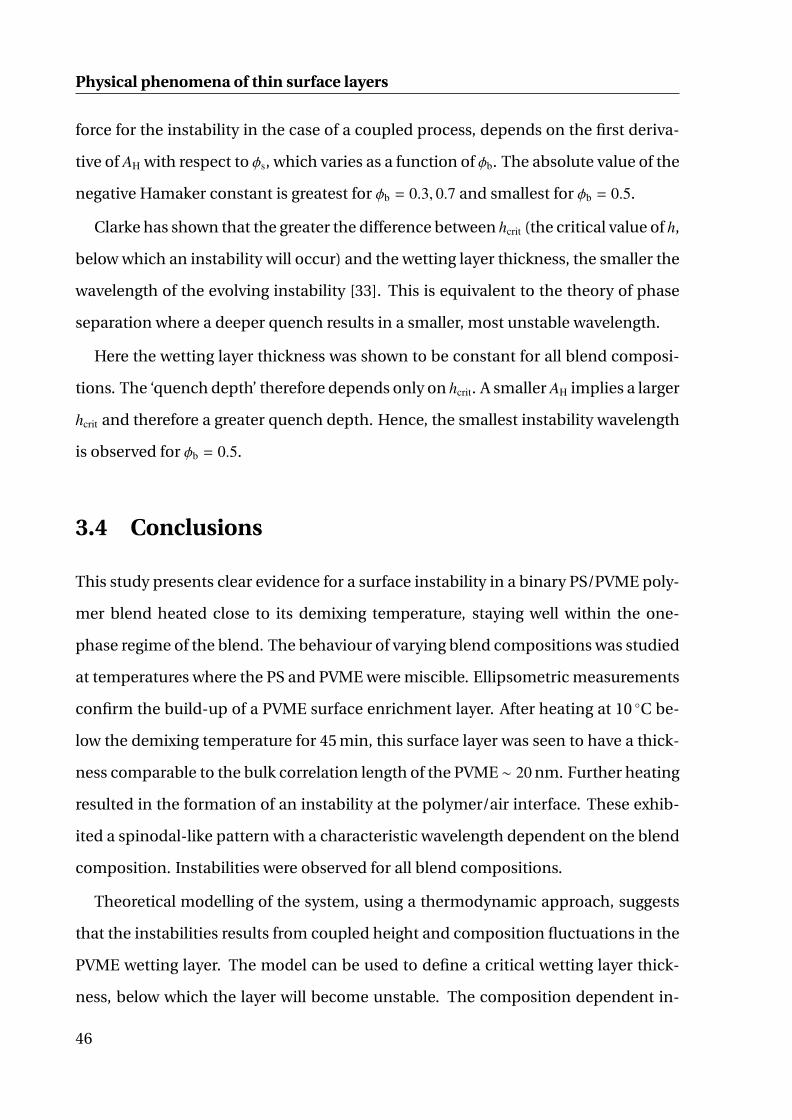
Physical phenomena of thin surface layers
force for the instability in the case of a coupled process, depends on the first deriva-
tive of AH with respect to φs, which varies as a function of φb. The absolute value of the
negative Hamaker constant is greatest for φb = 0.3, 0.7 and smallest for φb = 0.5.
Clarke has shown that the greater the difference between hcrit (the critical value of h,
below which an instability will occur) and the wetting layer thickness, the smaller the
wavelength of the evolving instability [33]. This is equivalent to the theory of phase
separation where a deeper quench results in a smaller, most unstable wavelength.
Here the wetting layer thickness was shown to be constant for all blend composi-
tions. The ‘quench depth’ therefore depends only on hcrit. A smaller AH implies a larger
hcrit and therefore a greater quench depth. Hence, the smallest instability wavelength
is observed for φb = 0.5.
3.4 Conclusions
This study presents clear evidence for a surface instability in a binary PS/PVME poly-
mer blend heated close to its demixing temperature, staying well within the one-
phase regime of the blend. The behaviour of varying blend compositions was studied
at temperatures where the PS and PVME were miscible. Ellipsometric measurements
confirm the build-up of a PVME surface enrichment layer. After heating at 10 C be-
low the demixing temperature for 45 min, this surface layer was seen to have a thick-
ness comparable to the bulk correlation length of the PVME ∼ 20 nm. Further heating
resulted in the formation of an instability at the polymer/air interface. These exhib-
ited a spinodal-like pattern with a characteristic wavelength dependent on the blend
composition. Instabilities were observed for all blend compositions.
Theoretical modelling of the system, using a thermodynamic approach, suggests
that the instabilities results from coupled height and composition fluctuations in the
PVME wetting layer. The model can be used to define a critical wetting layer thick-
ness, below which the layer will become unstable. The composition dependent in-
46

Wetting induced instabilities in miscible polymer blends
stability wavelength, arises from the dependence of the Hamaker constant on both
the bulk and wetting layer compositions. The Hamaker constant defines the critical
wetting layer thickness. Since the experimentally observed PVME wetting layer has
the same thickness for all blend compositions, the Hamaker constant determines the
‘quench depth’ of the system. The greater the difference between the critical layer
thickness and the wetting layer thickness, the smaller the wavelength of the resulting
instability.
Instabilities were only observed in blends heated close to the demixing tempera-
ture. PVME-rich wetting layers were also observed to form at the polymer/air inter-
face in blends kept at room temperature for extended periods of time. These blends
were stable however and no instabilities were seen to evolve.
47


CHAPTER
FOUR
OUT OF EQUILIBRIUM DYNAMICS OF THIN POLYMER
FILMS
The process of spin coating to form thin films is widely used in polymer science and in
technological applications. The popularity of the technique stems from the ability to
form uniform films over large areas, with thicknesses ranging from a few nanometres
to a few micrometres.
A drop of polymer solution is placed onto a substrate, which is then rotated caus-
ing the solution to spread. The solvent rapidly evaporates, increasing the glass tran-
sition temperature Tg of the liquid film. When Tg reaches the ambient temperature,
the polymer vitrifies forming a glassy film. While the remaining solvent continues to
evaporate, the conformations of the chains within the film are frozen-in.
Films formed in this way are often seen to exhibit anomalous structural and dynam-
ic properties, which strongly differ from the bulk behaviour of the polymer [7, 98–100].
The properties of films are dependent on the film thickness, with a greater deviation
from bulk behaviour seen as the film thickness is decreased1. Films which are thicker
than 100 − 200 nm are generally considered to have bulk behaviour.
1The discussion here is limited to films thicker than the coil size of the polymer chain. For thinnerfilms, confinement effects of the polymer chain may start to play a role and must also be considered.
49
Physical phenomena of thin surface layers
a dcb
Figure 4.1: Optical micrographs of dewetting observed in a 40 nm PS film heated at 125 Cafter (a) 0 min (b) 1 min (c) 10 min (d) 60 min. PS Mw = 4000 kg mol−1 was spun from toluene at6000 rpm onto a silicon wafer coated with a 10 nm PDMS layer.
Thin polymer films have been shown to exhibit a negative thermal expansion co-
efficient when heated close to the glass transition temperature Tg [99]. As the film
thickness is decreased, the onset of this thickness contraction is seen to occur at lower
temperatures with T Tg [100].
Bulk equilibrium behaviour can be achieved for spin-cast films through thermally
annealing the films above Tg for an extended period of time [101]. Jones et al. have
shown that films annealed for times greater than the time required for the polymer
chain to diffuse a distance comparable to the radius of gyration Rg of the polymer,
have the same chain conformations as those observed in the bulk [102]. Films with
thicknesses of 10 − 100 nm have been investigated and no thickness dependence was
observed except for the thinnest films, where the thickness was comparable to Rg.
Kim et al. have shown that thermally annealed films have a viscosity equalling that of
the bulk viscosity of the polymer [103, 104].
The difference in behaviour is thought to arise from non-equilibrium conforma-
tions of the polymer chains and frozen-in stresses, resulting from the preparation of
the films from solutions by rapid solvent evaporation. A popular method of inves-
tigating the behaviour of thin polymer films is through studying the dewetting of a
polymer film on a substrate [105]. The dewetting process can be explained in terms
of non-equilibrium chain conformations and entanglements in thin polymer films,
the relaxation of which can be probed in situ in real time. In dewetting experiments,
50

Out of equilibrium dynamics of thin polymer films
0 50 100 1500
10
20
N max (
hole
s pe
r 104 µ
m2 )
tageing (h)
a b
Figure 4.2: (a) Number of holes which spontaneously nucleate in PS films aged at 50C forvarious times. The insets show typical micrographs. (b) Evolution of the dewetting velocityand rim width for a PS film. τw indicates the timescale on which residual stresses relax, whileτv indicates the timescale on which equilibration of the film takes place. Graphs taken from[106] and [107] respectively.
the film is heated to T > Tg after spin casting. Upon annealing, holes form and grow.
An example of this can be seen in figure 4.1. The shape of the rim and the growth
velocity of the holes can be interpreted in terms of molecular, interfacial and rheo-
logical properties of the film. Films which are aged below Tg show a decreasing num-
ber of spontaneously nucleated holes per unit area are observed upon heating above
Tg [106] (figure 4.2a). After a sufficiently long period of aging, it is predicted that holes
will no longer form in an idealised polymer film.
The change in rupture probability is a signature of the metastability and non-
equilibrated chain conformations of the films and suggests higher stresses in the as-
spun films as compared to the aged films. Residual stresses, which can be stored in
the films due to distorted chain conformations, provide an additional driving force
for dewetting, thereby accelerating the process [108]. As the films are aged, these
stresses relax as the polymer chains adopt conformations closer to equilibrium and
the holes stop growing (figure 4.2b). The results suggest that the anomalous be-
haviour observed in as-cast films originates from the film preparation and can be
removed by aging below Tg.
51

Physical phenomena of thin surface layers
Dewetting experiments can also be used to probe the rheology of the films. The
velocity of the dewetting front gives an indication of the viscosity of the fluid. See-
mann et al. have shown that the viscosity is significantly reduced, compared to the
bulk, in as-cast PS films [19]. Masson et al. show a similar viscosity reduction but
only for films with a thickness less than 80 nm [101]. A transition in the dewetting ve-
locity is observed on timescales greater than the relaxation of residual stresses [107].
This is shown in figure 4.2b and suggests that residual stresses may relax without full
equilibration of the polymer chains, which requires the film to be annealed at T > Tg.
While dewetting experiments give insight into the non-equilibrium properties of
as-cast films or films aged below Tg, fully equilibrated films cannot be probed due to
the unstable nature of the films. Barbero et al. have shown that electric fields can be
used to perturb the free surface of a polymer film heated above Tg in order to probe
the rheology of the liquid film [7]. In these experiments the films are intrinsically
stable in the absence of the destabilising force, allowing for the direct comparison of
as-cast with equilibrated films.
Electric field destabilisation provides an ideal way to study the behaviour of liquid
polymer films due to the ability to disentangle the force balance driving the instabil-
ity from the rheology within the film, which is not possible in dewetting experiments.
The magnitude of the characteristic wavelength λ of the instabilities reflects the bal-
ance of forces acting on the surface of the film and is not dependent on the film rheol-
ogy as long as the flow in the film can be considered to be laminar. The characteristic
onset time τ of the instabilities however, is proportional to the viscosity of the film.
Figure 4.3 shows the characteristic destabilisation time of the film as a function of
the instability wavelength for PS with different molecular weights Mw, as measured
by Barbero [7]. As-cast films are observed to have a substantially reduced viscosity as
compared to the bulk (figure 4.3a,c,e). Annealing the films above Tg, for sufficiently
long times prior to destabilisation, results in an increase in the measured viscosity,
with bulk viscosity being recovered (figure 4.3b,d).
52

Out of equilibrium dynamics of thin polymer films7.5. NON-EQUILIBRIUM CHAIN CONFORMATIONS 101
4 5 6 7 8 90
05
001
051
002
052
λ ( μ )m
τ (m
in)
PS10= 15 V ( )= 18 V ( )= 121 nm= 128.5 °C
UUh T
01 02 03010
012
014
016
018
λ ( μ )m
τ (m
in)
as spun S655P
λ ( μ )m
τ (m
in)
9 01 11 21 310
001
002
003
004
005
λ ( μ )m
τ (m
in)
4 5 6 7 8 90
002
004
006
008
λ ( μ )m
τ (m
in)
c
a b
3 4 5 6 70
05
001
051
002
052
003
λ ( μ )m
τ (m
in)
d
fe
as spun S27.5P
as spun S113P
annealed S27.5P
annealed S113P
5 7 9 11 13 150
200
400
600
800Uh T
= 25 V= 135 nm= 142 °C
Uh T
= 5 V = 90 nm= 191 °C
Uh T
= 14 V= 103 nm= 169 °C
Uh T
= 16 V= 93 nm= 167 °C
Uh T
= 14 V= 148 nm= 142 °C
Uh T
= 12 V= 168 nm= 142 °C
Figure 7.4: Characteristic destabilization time τ as a function of instabilitywavelength λ for 4 polymer molecular weights. a, c and b, d compare filmsbefore and after annealing for PS27.5 and PS113, respectively. The circles andsquares in a correspond to films on bare silicon wafers and surfaces covered by aself-assmbeled monolayer, respectively. The squares and circles in b correspondto two samples of different thicknesses. The squares and circles in f correspondto annealed and as-cast samples, respectively. The dashed lines are predictionsof equation 7.1 using the bulk viscosity, the solid lines are fits of equation 7.1 tothe data by variation of η (Table 7.2). The error of measurement of λ is ∼10%(not shown on the graphs)
.
Figure 4.3: Characteristic destabilisation time τ vs. wavelength λ. (a),(c) and (b),(d) com-pare films before and after annealing. The different symbols in (a) correspond to bare andfunctionalised substrates, (b) samples of different thicknesses, (f) annealed and as-cast films.Dashed lines are the predictions using the bulk viscosity, the solid lines are fits found by vary-ing the viscosity. Graphs taken from [7].
The destabilisation of films with Mw = 10 kg mol−1 does not show this effect (figure
4.3f). The Mw of this polymer is below the entanglement molecular weight of PS. Here
the data for the as-cast and annealed films are both described by the bulk viscosity.
53

Physical phenomena of thin surface layers
Similar behaviour is observed by Yang et al. who investigated the viscosity of PS films
with Mw = 2.4 kg mol−1 via spinodal decomposition of the films [109].
Barbero [110] also looked at the role of the film/substrate interface on the proper-
ties of the film. A reduction in the characteristic onset time is predicted if there is fi-
nite slip at the liquid/solid interface, which could be the cause of the observed reduc-
tion in viscosity. The results are shown in figure 4.3a, where films spun onto cleaned
silicon wafers are compared to those spun onto surface-functionalised wafers, which
have a substantially reduced interfacial energy with the PS. The results show that
the characteristic destabilisation times for the two sets of films are indistinguishable.
This indicates that the solid boundary does not play a significant role during the early
stage of destabilisation and interfacial slip is not the cause of the increased mobility
observed in the as-cast films.
The reduced effective viscosity is instead explained in terms of entanglements of
the polymer chains. In the initial phase of spin coating, the polymer is in a semi-dilute
solution with a good solvent. As the solvent evaporates the chains start to entangle.
As the polymer concentration increases further, this process slows and stops once
the film vitrifies. This results in a lower entanglement density per chain and therefore
lower viscosity than seen for a fully equilibrated film. Annealing at T > Tg equili-
brates the chains, restoring the melt entanglement density and viscosity. This model
is corroborated by Tsui et al., who show that in high Mw PS, the elastic modulus of the
polymer in spin coated films is substantially reduced compared to bulk PS [111]. This
again suggests the chains have a lower entanglement density and did not have time
to fully interpenetrate before vitrification.
This chapter builds on the work of Barbero, using electrohydrodynamic (EHD)
destabilisation to explore the effect of the solvent used for spin-casting on the prop-
erties of the film produced. Both the viscosity and the residual stresses in the film
are studied. Particular attention is paid to the timescale on which these stresses re-
lax. Solvent vapour annealing is used as an alternative method to thermal annealing,
54

Out of equilibrium dynamics of thin polymer films
to achieve fully equilibrated films on much shorter timescales. In tandem with this
study, similar experiments were carried out by Adam Raegen and Günter Reiter at
the University of Freiburg, where the effect of casting solvent on the dewetting of PS
films was investigated. The results of these experiments are discussed and compared
to those of the EHD destabilisation study.
55

Physical phenomena of thin surface layers
Solvent Tbp (C) Tm (C) η (25 C) ϕsolvent
Trans-decalin (TD) 187 -31 1.948 0.46 (0.3)Toluene 110 -95 0.560 0.23Chloroform 61.2 -64 0.537 0.32Methyl ethyl ketone (MEK) 79.6 -87 0.405 0.25Tetrahydrofuran (THF) 66 -45 0.456 0.30
Table 4.1: Boiling point Tbp, melting point Tm, viscosity η and concentration of solvent ϕsolventat vitrification of the polymer for the solvents used for spin coating. Physical data taken from[86]. ϕsolvent for TD is shown for 25 C (55 C).
4.1 Materials and methods
Polystyrene (PS) Mw = 200 kg mol−1 (PS200), Mw/Mn = 1.09 (Polymer Source), PS Mw =
655 kg mol−1 (PS655), Mw/Mn = 1.09 (Polymer Source) and PS Mw = 4000 kg mol−1 (PS4000),
Mw/Mn = 1.15, (Polymer Standards Service) were used as obtained without further
purification. The glass transition of the three polymers is at ∼ 105 C 2. The dielectric
constant of PS is 2.5 [86], this is unchanged on application of a DC electric field [112].
The PS films were spin coated onto cleaned silicon substrates from solution with a
spin speed of 4500 rpm. The solvents used and their properties are given in table 4.1.
Films spun from trans-decalin (TD) solutions were spun at 55 C and 25 C. For all
other solvents films were formed at room temperature. After spin coating, all sam-
ples were annealed at 60 C for 15 min to remove any residual solvent.
Spin coating is a commonly used technique to coat substrates with thin polymer
layers. The substrate is coated with droplets of the solution and is subsequently ro-
tated at a given speed. On rotation of the substrate, the solution spreads out forming
a liquid layer. Once a homogeneous film thickness across the substrate is established,
thinning of the liquid layer occurs mainly by solvent evaporation, with draining of the
solution across the edge becoming negligible. The spreading of the liquid and the rate
of thinning are dominated by viscous forces and the boiling properties of the solvent,
assuming that the spinning speed is constant. Films spun from TD, which has a high
2Physical data as determined by the supplier.
56

Out of equilibrium dynamics of thin polymer films
0.2 0.4 0.6 0.8
180200220240260280300320340360
T g (o K)
φsolventpolymer
Figure 4.4: Variation of Tg for PS in Toluene (solid), TD (dotted), chloroform (short-dash),MEK (long-dash) and THF (dash-dot) as a function of ϕpolymer according to equation 4.1. Ver-tical dashed line indicates ϕpolymer at 300 K.
boiling point, were seen to form more slowly than those spun from tetrahydrofuran
(THF), which has a much lower boiling point.
When the solvent concentration reaches a critical value ϕsolvent, the polymer vitri-
fies, forming a smooth film. The critical solvent concentration is dependent on the
melting point of the solvent and the glass transition temperature of the polymer and
can be found using the Fox equation [113]
1Tg
=ϕsolvent
Tm+
1 − ϕsolvent
Tp(4.1)
where Tp is the glass transition temperature of the polymer and Tm is the melting point
of the solvent. Tg is the temperature at which the polymer vitrifies, which in this case
is 300 K. Figure 4.4 shows the variation in Tg as a function of ϕsolvent for each solvent
used. The graph was used to obtain the values for ϕsolvent given in table 4.1.
The final film thickness is dependent on a number of parameters including the
viscosity, the spin speed and the concentration of the initial polymer solution used.
Here the spin speed was kept constant. 1% and 3% solutions were used to form 100 nm
thick films for Mw = 4000 kg mol−1 and Mw = 200 kg mol−1 PS respectively. Films were
used as-cast, after annealing at Tanneal = 155 C or after solvent annealing. A vacuum
57

Physical phenomena of thin surface layers
sample chamber
solvent lines
a b
Figure 4.5: (a) Solvent vapour setup. (b) Sample chamber.
oven was used for thermal annealing to avoid degradation of the polymer.
Vapour annealing
The vapour annealing setup can be seen in figure 4.5. The films were placed in the
annealing chamber, which was then sealed and filled with solvent vapour of a given
concentration. The vapour causes the film to swell. All experiments were carried out
using toluene. The films were all initially swollen in an atmosphere containing 50%
toluene, followed by a step with a reduced toluene concentration. All films were dried
under nitrogen flow for 15 min after solvent annealing to remove any residual solvent.
The film thickness before and after vapour annealing was measured using ellip-
sometry, as discussed in chapter 3. The 100 nm films were seen to increase by 20−25 nm
during the vapour annealing process. After 5 mins in the solvent atmosphere the film
stopped swelling and the thickness remained constant for the rest of the annealing
time. The film thickness was unchanged after vapour annealing was finished, con-
firming that all solvent had been removed.
Destabilisation setup
The formation of electrohydrodynamic (EHD) instabilities was carried out using two
58

Out of equilibrium dynamics of thin polymer films
V
ITO glass
Silicon waferFilmAir gap
Film
Silicon wafer
Silicon wafer
V
Air gap
a
b
c d
e
f
Figure 4.6: Experimental setups. (a,b) Microscope setup. (c) Polymer film is sandwiched withan air gap between silicon and ITO glass electrodes. The ITO glass provides a transparent elec-trode for viewing. (d,f) Oven setup. (e) Polymer film is sandwiched with an air gap betweentwo silicon electrodes.
different experimental setups, which can be seen in figure 4.6. The oven setup (figure
4.6d,f) was used to investigate the change in wavelength as a function of the electric
field, while the microscope setup (figure 4.6a,b) was used to explore the onset time
of instability formation. It should be noted that while the schematic representations
shown in figure 4.6c,e show parallel capacitor plates, experimentally a small wedge
geometry was always achieved. The electric field is inversely proportional to the sep-
aration of the capacitor plates and as a result each sample could be used to obtain a
number of data points.
Silicon wafers (specific resistance = 6 − 10 Ω cm2) covered by a 40 nm gold layer on
their backside were used as negative electrodes. A 5 nm chromium layer was used to
adhere the gold to the wafer. The gold layer provided good electrical contact to the
copper plates used to assemble the devices. The wafers were attached to the copper
plates using a silver paste. Silicon wafers and indium-tin oxide (ITO) coated glass
(specific resistance = 80 − 100 Ω cm2) were used for the upper electrodes.
Photolithography
Photolithography was used to create SU8 spacers on the electrodes to provide an air
59
Physical phenomena of thin surface layers
gap between the polymer film and the upper electrode. SU8 2000.5 photoresist was
spun onto the cleaned silicon/ITO glass at a spin speed of 6000 rpm. The films were
temperature cured using the following procedure: heat at 60 C for 1 min, 100 C for
1 min, 60 C for 1 min. This heating procedure was carried out to remove residual sol-
vent, relax stresses in the photoresist and to promote adhesion with the substrate.
The resist film was aligned for photocuring using an MJB4 mask aligner. This al-
lows for selective exposure of the film with UV light through a mask. The masks were
made of UV-transparent quartz glass patterned with an absorber metal, in this case
chromium, which is opaque to UV light.
UV curing was carried out for 2 s. Upon exposure to UV light, the resist under-
goes changes in its chemical and physical properties which alter its solubility. Areas
masked by the chromium were left unchanged. The films were then post-baked for
1 min at 60 C, 1 min at 100 C and 1 min at 60 C to complete the chemical reaction.
The substrate was rinsed in SU8 developer, which selectively dissolves the unexposed
areas and rinsed in isopropanol. A final bake at 175 C for 2 min was carried out to re-
move and dry any developer residue.
Experimental conditions
The devices were assembled in the EHD setups at room temperature. The films were
heated to 175 C and the temperature was allowed to equilibrate. The equilibration
times were 20 min and 5 min for the oven and the microscope setup respectively. Once
the temperature had equilibrated, the electric field was turned on, defining the start
of the experiment (t = 0).
Figure 4.7 shows the effect on the measured wavelength of the instabilities as a
function of the applied electric field for the two different setups. In addition, devices
were placed into a pre-heated oven and the electric field turned on directly. No dif-
ference was seen in the resulting behaviour.
60

Out of equilibrium dynamics of thin polymer films
2.0x10⁷ 4.0x10⁷ 6.0x10⁷ 8.0x10⁷ 1.0x1082.0x10-6
4.0x10⁻⁶
6.0x10⁻⁶
8.0x10⁻⁶
1.0x10⁻⁵
1.2x10⁻⁵
Wav
elen
gth
[m]
Electric Field [V/m]
Figure 4.7: Variation in the wavelength of the instability as a function of the electric fieldfor a 100 nm PS=200 kg mol−1 film. () Oven setup. (N) Microscope setup. (•) Oven setup -preheated. The line is a guide for the eye.
4.1.1 Optical observation of instabilities
The microscope setup shown in figure 4.6a,b was used for in situ observation of the
EHD instabilities in real time. The electrodes were placed on a heated stage, mounted
on an inverted microscope. The white light from the halogen light source passed
through an interference filter, providing quasi-monochromatic illumination of the
sample. The mean wavelengths of the interference filters used were 515 nm and 532 nm.
The silicon wafer and ITO glass, used as electrodes, acted as an optical cavity. Inter-
ference fringes due to the recombination of light beams within the cavity were ob-
served. An example of the fringes is shown in figure 4.8a.
The use of light interference allowed for accurate observation of the onset of in-
stability formation. Initially the film was flat and appeared monochromatic (figure
4.8a). Interference fringes were observed due to the variation in the thickness of the
air gap, as a result of the wedge geometry of the setup. The formation of instabil-
ities results in local variation of the film thickness and a change in the intensity of
the reflected light (figure 4.8b). For a 3 nm variation in the thickness, the change in
intensity of the reflected light is on the order of 7 − 20% for the experimental config-
uration used here [110], depending on the position of the instability with respect to
61

Physical phenomena of thin surface layers
a b c
Figure 4.8: Example images showing the destabilisation of a PS film. (a) Initial uniform filmshowing interference fringes. (b) Onset of EHD instabilities. (c) Instabilities start to formcolumns. (b,c) Insets show magnification of selected area. Scale bar: 100 µm.
the interference fringes. This change in intensity allows the instability formation to
be easily observed using optical microscopy and the time taken for the instability to
reach a few nanometres in height to be easily measured. For a more detailed discus-
sion of the experimental setup and the use of light interference in an optical cavity to
measure film thickness and the growth of instabilities see [110].
Atomic force microscopy
The height and wavelength of the EHD instabilities formed in the oven were inves-
tigated using a Dimension 3100 Veeco atomic force microscope. Atomic force mi-
croscopy (AFM) was chosen due its nanometre resolution and non-destructive imaging.
AFM is a high-resolution imaging technique, which allows the topography and
composition of a surface to be imaged. Figure 4.9a shows a schematic representa-
tion of the AFM. AFM works by measuring the interactions between the sample and
the tip. In TappingMode™ or non-contact mode, the tip does not touch the sam-
ple. The cantilever is driven at its resonance frequency and a feedback loop is used to
maintain a constant amplitude of the cantilever. Topographic and phase images are
derived from measurements of the attractive force between the tip and the sample
due to deflections of the tip as it is scanned across the surface. These deflections are
measured using a laser focused onto the backside of the cantilever.
AFM can also be used in contact mode. This can however, damage the sample.
62

Out of equilibrium dynamics of thin polymer films
LaserPhotodiode
Cantilever
Tip
SampleStage a b
Figure 4.9: (a) Schematic representation of AFM. (b) Dimension 3100 Veeco AFM used in thisstudy.
Only non-contact mode was used here. AFM was also used for roughness measure-
ments and to observe the phase separation of PS/PVME films as discussed in chapter
3. For a more detailed discussion on AFM see [114].
63

Physical phenomena of thin surface layers
Figure 4.10: Onset and growth of EHD instabilities in PS200 spun from trans-decalin. Scalebar is 20 µm.
4.2 Results and discussion
The application of an electric field across the polystyrene (PS) film heated at T > Tg
resulted in the destabilisation of the film and the evolution of a surface wave with a
characteristic wavelength. An example of this for a film spun from trans-decalin is
shown in figure 4.10.
4.2.1 Toluene
Film rheology
The characteristic onset time τ as a function of the wavelength of the instability is
given by
τ =3ηγh3
0
(λ
2π
)4
(4.2)
where h0 is the thickness of the initial film. The onset time is proportional to the
viscosity η and inversely proportional to the surface tension γ of the liquid film.
Figure 4.11 shows the onset times for EHD instabilities observed in PS200 films
spun from toluene, as measured using the optical setup. Data were obtained for films
destabilised directly after spin coating and for films annealed for 140 hrs at Tanneal = 155 C
prior to destabilisation. From figure 4.11 it can be seen that the characteristic onset
64

Out of equilibrium dynamics of thin polymer films
2 3 4 5 60
10
20
30
40
50
60
70
80
τ [m
in]
λ [µm]
Figure 4.11: Characteristic destabilisation time τ vs λ for (•) as-spun films and after annealingat Tanneal for () 30 hrs, (⊕) 70 hrs, () 96 hrs and () 140 hrs. Lines show fits to the data usingequation 4.2 with η = 30, 35, 65, 90, 110 kPa · s.
time τ is greatly reduced in the as-spun films. This corresponds to an increase in the
mobility of the film.
From equation 4.2 it can be seen that changes in τ may result from changes in γ,
εp and/or η. The dielectric constant εp of PS is 2.5 [86]. Park et al. have shown that
the application of a high DC field to a polymer film, similar to those used here, does
not change the measured value of εp [112]. The surface tension of PS is γ = 27.5 −
36.0 mN/m at temperatures between 130 C and 200 C. The surface tension is both
temperature and molecular weight dependent. For Mw = 200 kg mol−1, γ ' 35 mN/m
at 175 C [115]. The experiments here were carried out at constant temperature and
applied voltage. Small fluctuations in γ and εp do not account for the large decrease
in τ demonstrated in figure 4.11.
Barbero et al. have shown that the only likely parameter that can be used to explain
the observed decrease in τ is the viscosity of the liquid film [7]. The curves in figure
4.11, show fits to the data using equation 4.2, assuming viscosities of 30 kPa · s for the
as-spun film and 110 kPa · s for the film annealed for 140 hrs. The latter corresponds
closely to η = 127 kPa · s, the bulk viscosity of the polymer3.
In figure 4.3 the data for large λ lie above the curve fitted to the data at small λ. Bar-
3The viscosity of the bulk polymer was measured using a parallel plate rheometer.
65

Physical phenomena of thin surface layers
bero suggests that this is due to chain relaxation during the experiment. This is not
observed in the data shown here. These experiments were conducted at higher ap-
plied voltages and therefore electric fields than those of Barbero. The onset of desta-
bilisation was observed on timescales of 2 − 80 min. Using a similar Mw PS, Barbero
observed destabilisation on a timescale of 20 − 220 min, with a deviation in the fit be-
ing observed after 120 min (figure 4.3c), which is much greater than the length of the
experiments conducted here.
A small increase in τ was observed after 30 hrs of annealing at Tanneal prior to desta-
bilisation. The characteristic onset times for the EHD instabilities observed after
30 hrs of annealing are shown in figure 4.11. An increase in the viscosity of ∼ 5 kPa · s is
measured. Full equilibration and the recovery of bulk properties however, occurs af-
ter much longer annealing times. The time dependence of the relaxation is discussed
later in this chapter.
The recovery of bulk viscosity in the films on annealing above Tg suggests that the
increased mobility observed in the as-cast films results from non-equilibrium effects
caused by the spin coating film deposition procedure. Annealing of the films for suf-
ficiently long times removes this non-equilibrium effect.
Residual stresses
The characteristic wavelength λ of the instabilities as a function of the applied electric
field is given by
λ = 2π
√2γU
ε0εp(εp − 1)2 E−3/2p (4.3)
and gives an indication of the forces and residual stresses acting on the film. Figure 4.12
shows the characteristic wavelength of fully formed instabilities as a function of the
applied electric field for PS4000. The line shows the theoretical prediction of equa-
tion 4.3. Films annealed for 140 hrs are well described by equation 4.3. For as-cast
films however, the values of λ are systematically higher. Figure 4.12 also shows values
66

Out of equilibrium dynamics of thin polymer films
1x10⁷ 2x10⁷ 3x10⁷ 4x10⁷ 5x10⁷ 6x10⁷ 7x1070
4
8
12
16
20
λ[µm
]
Ep [V/m]
Figure 4.12: Characteristic wavelength as a function of the applied electric field for (•) as-spunand films annealed for (⊕) 1 hr (⊗) 10 hrs and () 140 hrs at Tanneal. Line shows the prediction ofequation 4.3.
of λ for films annealed for 1 hr and 10 hrs at Tanneal prior to destabilisation. The recovery
of bulk behaviour here is observed much faster than the recovery of bulk viscosity.
It has been shown that non-equilibrium chain conformations result in additional
in-plane stresses in spin-cast films [116]. These are seen to drive destabilisation and
hole formation in dewetting experiments [106]. Assuming that the same in-plane
stresses are present in these films, they should also act as an additional driving force,
resulting in smaller values of λ and faster τ. This however, is not seen. The larger
values of λ in the as-cast films are instead indicative of a stabilising pressure acting
on the as-cast films. A similar effect was observed by Barbero for PS Mw = 113 kg mol−1
and 27.5 kg mol−1 [110].
One possible explanation for the behaviour observed in the as-cast films is frozen-
in normal stresses. These could result from strong solvent gradients during spin coat-
ing, which lead to a variation in the entanglement density of the chains normal to
the film surface. Polymer adsorption at the substrate could also give rise to a non-
equilibrium conformation at the polymer/substate interface.
A comparison of the characteristic wavelength of the instabilities for as-spun PS
films with Mw = 4000 kg mol−1 and 200 kg mol−1 can be seen in figure 4.13a. Films
67

Physical phenomena of thin surface layers
1x10⁷ 2x10⁷ 3x10⁷ 4x10⁷ 5x10⁷ 6x10⁷ 7x1070
4
8
12
16
20
λ[
µm]
Ep [V/m] b c
a
Figure 4.13: (a) Characteristic wavelength of instabilities as a function of the applied electricfilm for as spun films. (•) PS4000 and (N) PS200. Schematic representation of the deformationof a polymer chain swollen in toluene with a given density of segments on loss of the solventfor (b) a low molecular weight and (c) a higher molecular weight polymer.
spun from PS200 have a reduced wavelength compared to those spun from PS4000.
Shorter wavelength instabilities, for both polymers, are observed to have a greater
deviation from bulk behaviour than longer-wavelength instabilities. Bulk behaviour
is observed for PS200 for λ > 15 µm.
Longer-wavelength instabilities are observed for smaller applied electric fields and
have increased onset times as compared to shorter-wavelength instabilities. The
films are heated above Tg during the incubation time before instability onset. From
equation 4.2 it can be seen that longer wavelengths imply much greater incubation
times before instability onset, giving the film more time to relax stresses arising from
spin-coating. For PS200 relaxation of the frozen-in stresses occurs on much shorter
timescales than for PS4000.
The data shown in figure 4.13a are in agreement with the hypothesis that frozen-
in normal stresses are responsible for the non-equilibrium behaviour observed here,
since the magnitude of the stresses is greater for the higher molecular weight poly-
mer. Consider the liquid films during the spin coating process just prior to vitrifica-
tion. Taking first the PS200, each chain can be considered to occupy a sphere of radius
r200 with a given segment density. After vitrification the remaining solvent evaporates
68
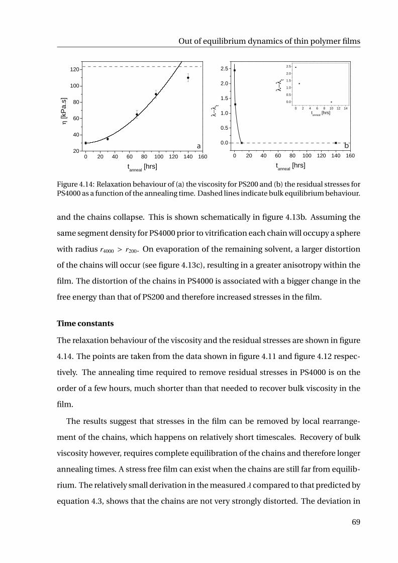
Out of equilibrium dynamics of thin polymer films
0 20 40 60 80 100 120 140 16020
40
60
80
100
120
η [k
Pa.
s]
tanneal [hrs]0 20 40 60 80 100 120 140 160
0.0
0.5
1.0
1.5
2.0
2.5
λ−λ t
tanneal [hrs]
0 2 4 6 8 10 12 14
0.0
0.5
1.0
1.5
2.0
2.5
λ−λ t
tanneal [hrs]
a b
Figure 4.14: Relaxation behaviour of (a) the viscosity for PS200 and (b) the residual stresses forPS4000 as a function of the annealing time. Dashed lines indicate bulk equilibrium behaviour.
and the chains collapse. This is shown schematically in figure 4.13b. Assuming the
same segment density for PS4000 prior to vitrification each chain will occupy a sphere
with radius r4000 > r200. On evaporation of the remaining solvent, a larger distortion
of the chains will occur (see figure 4.13c), resulting in a greater anisotropy within the
film. The distortion of the chains in PS4000 is associated with a bigger change in the
free energy than that of PS200 and therefore increased stresses in the film.
Time constants
The relaxation behaviour of the viscosity and the residual stresses are shown in figure
4.14. The points are taken from the data shown in figure 4.11 and figure 4.12 respec-
tively. The annealing time required to remove residual stresses in PS4000 is on the
order of a few hours, much shorter than that needed to recover bulk viscosity in the
film.
The results suggest that stresses in the film can be removed by local rearrange-
ment of the chains, which happens on relatively short timescales. Recovery of bulk
viscosity however, requires complete equilibration of the chains and therefore longer
annealing times. A stress free film can exist when the chains are still far from equilib-
rium. The relatively small derivation in the measured λ compared to that predicted by
equation 4.3, shows that the chains are not very strongly distorted. The deviation in
69

Physical phenomena of thin surface layers
Expa
nsio
n Fa
ctor
(α)
2015 25 30 35 40 45 500
0.2
0.4
0.6
0.8
1.0
1.2
1.4
T ( C)o
Figure 4.15: Chain conformation of PS chains in TD as a function of the solution tempera-ture. Mw = (solid) 200 kg mol−1 (dotted) 1000 kg mol−1 (short-dash) 4000 kg mol−1 (long-dash)16800 kg mol−1.
viscosity is much larger indicating that the chains are far from equilibrium. Note that
the reptation times for PS4000 at 175 C ≈ 3·104 s and for PS200 at 175 C ≈ 4 s [117] are
much smaller than the relaxation time required for full equilibration of the films, also
indicating the non-equilibrium nature of the spin-cast films. This will be discussed
further in section 4.2.4. The relaxation of the residual stresses for PS4000 is on the
order of the reptation time.
4.2.2 Trans-decalin
Trans-decalin is a θ-solvent with a θ-temperature θT ' 21 C. Below θT PS is not soluble
in TD and falls out of solution. Increasing the temperature above θT increases the
solubility of PS, with TD behaving as a good solvent at sufficiently high temperatures.
For a θ-solvent the degree of swelling of the chains is a function of the temperature
of the solution [118]. The dependency is given by
[14
3Nα3min
(α3 − α5) +23α3
min
α3
]/σ =
θ
T− 1 (4.4)
where α = 〈R2g〉
1/2/〈R20〉
1/2 is the expansion factor, R0 is the radius of gyration under
70

Out of equilibrium dynamics of thin polymer films
ideal melt conditions, αmin is the volume of the chains in the fully collapsed state and
σ is defined as σ = 1 − ∆S/kB with ∆S being the entropic change associated with
segment-segment interaction of the polymer.
Figure 4.15 shows the change in conformation of the PS chains as a function of
the solution temperature for various molecular weights of PS. Below θT, TD acts as a
poor solvent. The attractive intramolecular forces dominate and the chain contracts
forming a collapsed globule. The radius of gyration of the polymer follows [119]
Rg ∼ N1/3∣∣∣∣∣Tθ − 1
∣∣∣∣∣−1/3
for T < θ (4.5)
Above θT TD acts as a good solvent, the chains appear swollen and the volume they
occupy increases. In this case interactions between the monomers and the solvent
dominate over intramolecular forces. The conformation of the coils is described by
Rg ∼ N3/5∣∣∣∣∣Tθ − 1
∣∣∣∣∣1/5 for T > θ (4.6)
At θT intermolecular polymer-solvent repulsion exactly balances intramolecular monomer-
monomer attraction. Under these conditions the polymer behaves like an ideal chain
with
Rg ∼ N1/2 for T = θ (4.7)
Due to this ability to change the polymer-solvent interactions PS solutions in TD pro-
vide a tuneable system, allowing the conformation of the chains to be easily adjusted.
By varying the temperature at which the films are prepared the effect of the initial coil
conformation in the solvent on the properties of the films can be studied. Toluene is
a very good solvent and can therefore be compared to trans-decalin solutions at very
high temperatures.
71

Physical phenomena of thin surface layers
2 3 4 5 60
10
20
30
40
50
τ [m
in]
λ [µm]2 3 4 5 6
0
10
20
30
40
50
τ [m
in]
λ [µm]
Figure 4.16: Characteristic destabilisation time τ vs λ for as-spun films spun from (•) toluene,trans-decalin at () 55 C and () 25 C and () annealed films spun from trans-decalin. Linesshow fits to the data using equation 4.2.
Film rheology – solvent effects
Figure 4.16 shows a comparison of τ for films spun from trans-decalin(TD) at ∼ 25 C
(TD25) and ∼ 55 C (TD55) and those spun from toluene. A clear difference in the
onset time for the three sets of films is observed.
The onset of destabilisation is observed at shorter times in films spun from TD
than in films spun from toluene as shown in figure 4.16. For films spun from TD,
the onset time depends on the temperature at which the films were prepared, with
films prepared at 55 C (TD55) having longer onset times than those prepared at 25 C
(TD25). Annealing of TD films at Tanneal = 155 C for 140 hrs results in a recovery of
bulk behaviour. The unannealed data are described well by equation 4.2, assuming
η = 25 kPa · s for TD55 and η = 20 kPa · s for TD25. These results are in agreement
with the hypothesis that non-equilibrium chain conformations give rise to a reduced
viscosity.
From equation 4.4 and figure 4.15 it can be seen that for PS in toluene the chains
will be swollen, while for PS in TD at 25 C the radius of gyration of the chains is re-
duced. In [7] the reduced viscosity of toluene is explained in terms of entanglements
of the polymer chains. In the initial stages of spin coating, once the concentration
72

Out of equilibrium dynamics of thin polymer films
hypothesis, films cast from PS27:5 and PS113 were heated atT > Tg for times between 22 and 145 h (Table I). The
comparison of destabilization experiments in Fig. 2(b) withthe prediction of Eq. (3) confirms that bulk viscosity in thefilms is recovered after annealing. The good agreement ofexperiments and prediction validates our experimental ap-proach. It also indicates that high molecular weight poly-mer chains in spin-cast films have a quenched structure thatgives rise to a significantly lowered effective viscosity. Thelong time annealing of the film removes this nonequilib-rium effect. The destabilization of PS10 films which have aMw below the entanglement molecular weightMe of PS inFig. 2(f) does not show this effect: the data for as-cast andannealed films are both described by the bulk viscosity.
The sketch in Fig. 3 illustrates a possible mechanismthat is able to account for the nonequilibrium behavior inspin-cast films. In the initial phase of spin coating thepolymer forms a semidilute solution in a good solvent.During spinning, the solvent rapidly evaporates, increasingthe polymer concentration in the film. In thermal equilib-rium, the number of entanglements per chain with sur-rounding chains increases with polymer concentration.This leads to an increasingly entangled semidilute solutionwith decreasing solvent concentration. Since this increasein entanglements can only occur by chain reptation, themobility of the chains must be high enough for the entan-glement density to increase further. With increasing poly-mer concentration this process is progressively sloweddown and comes to a stop when the glass transition ofthe coils is reached. At this point, the film still containsð10–20Þ%vol solvent, which mostly evaporates during thelate stage of spin coating [16]. The slowdown of chainmobility and chain collapse is therefore likely to give riseto an entanglement density per chain which is lower com-pared to the melt equilibrium. Since the melt viscosity ofpolymers arises from the entangled nature of the chains,this qualitatively explains the lowered effective viscosity ofthe as-cast films. Annealing the film at T > Tg for times
exceeding the reptation time equilibrates the chains to theirfully entangled nature of the equilibrated melt.
The results in Fig. 2 indicate that the times requiredto destabilize the films were below the relaxation timesof the chains. Careful examination of the data in Figs. 2(a)and 2(c) shows that the data for large values of (low
applied electric fields) lie above the curve fitted to thedata with small . This is probably due to chain relaxa-tion during the experiment. This effect is better seenwhen plotting the two PS113 data sets in terms of thestress-strain relation in Fig. 4(a) for the onset of the insta-bility. The lateral stress arises from the difference in pres-sure [Eq. (1)]: ¼ 2½pðhmaxÞ pðhminÞ, where hmax, hmin
correspond to lateral locations x of adjacent undulationmaxima and minima. This pressure difference gives riseto a relative thickness change of 2h ¼ hmax hmin over alateral distance =2 during the time interval , defining thestrain rate.The linear stress-strain relation extracted from the data
in Fig. 2(d) for the annealed PS113 films is characteristic fora Newtonian liquid [15] with a viscosity of ¼ 29 kPa s,in good agreement with the literature value (Table I). Thedata of Fig. 2(c), for the as-cast film, on the other hand,shows a nonlinear stress-strain variation with a muchsmaller slope. In this representation, high strain rates cor-respond to small values of , while long destabiliza-tion times give rise to low strain rates. The lowest valueof the slope at high strain rates corresponds to the muchlowered effective viscosity of the data in Fig. 2(c) forsmall values of (high destabilizing fields). The increasein slope (i.e., increase in viscosity) with decreasing strainrate (i.e., low fields and high values of ) is indicative of anincrease in relaxation of the quenched polymer chains,giving rise to increasing values of the effective viscosity.The two curves approach each other in the limit of very lowstrain rates.The connection between the reduction in entanglement
density of the chains in the as-cast films and their loweredviscosity can be quantified in terms of the reptation model[17], ¼ 0ðMw=MeÞ with the intrinsic viscosity of theunentangled melt 0. Comparing two polymer melts withthe same chain length but different degrees of entangle-ment, Me and M0
e, can therefore be described by therelation M0
e=Me ¼ ð0=Þk, with k ¼ 1=ð 1Þ. Usingthe commonly accepted values of ¼ 3:4 and Me 17 kg=mol for PS, an increase in M0
e to 29 kg=moland 36 kg=mol account for the effective viscosity de-crease in the PS27:5 and PS113 films, respectively.The viscosity reduction in our experiments is likely to
arise from a reduced entanglement density. However, an-
FIG. 3 (color online). Model for the reduction in effective viscosity in spin-cast films. (a) Starting from a semidilute solution, (b) thechains start to entangle as the concentration increases. (c) The slowdown and collapse of the chains for high polymer concentrationsprevents the full equilibration of the chains. Thermal annealing equilibrates the chains, restoring the melt entanglement density (d).
PRL 102, 248303 (2009) P HY S I CA L R EV I EW LE T T E R Sweek ending19 JUNE 2009
248303-3
Figure 4.17: Schematic representation of the model used to describe the reduction in the ef-fective viscosity in spin-cast films. (a) Starting from a semi-dilute solution, (b) solvent evap-orates and the chains start to entangle as the concentration increases. (c) The slowdown andcollapse of the chains for high polymer concentrations prevents the full equilibration of thechains. Thermal annealing equilibrates the chains, restoring the melt entanglement density(d). Figure taken from [7].
of PS reaches the overlap concentration, the PS can be described as being in a semi-
dilute solution in toluene, a good solvent. At this point entanglement of the chains
starts to occur. As the solvent evaporates the polymer concentration in the liquid
film increases, which leads to an increasingly entangled semi-dilute solution. The
increase in entanglements occurs via chain reptation. As the solvent concentration
decreases, so the mobility of the chains decreases. Chain reptation is progressively
slowed and stops upon vitrification of the polymer. The resulting entanglement den-
sity of the chains is lower than that in a polymer melt at equilibrium. This is shown
schematically in figure 4.17. Melt viscosity comes from the entangled nature of the
chains. A lower entanglement density can therefore be used to explain the lower ef-
fective viscosity observed here.
For PS in trans-decalin at T ∼ θT the behaviour is similar now however, the PS is in a
near-θ solvent. As the solvent evaporates the PS will again form a semi-dilute solution
however, the polymer concentration at which this occurs is higher than that for a
good solvent due to the reduced Rg of the polymer. Once the overlap concentration is
reached, the chains start to entangle, with the entanglement density increasing with
polymer concentration. For toluene, vitrification occurs when the concentration of
solvent in the film decreases to ϕsolvent ∼ 0.23 (see table 4.1). For TD at θT this occurs
at ϕsolvent ∼ 0.46 resulting in a lower entanglement density of the chains and a reduced
73

Physical phenomena of thin surface layers
2x10⁷ 3x10⁷ 4x10⁷ 5x10⁷ 6x1070
4
8
12
16
20
λ[µm
]
Ep [V/m]
Figure 4.18: Characteristic wavelength of instabilities for as-spun films prepared from(•) toluene () TD25 and () TD55 . Line shows the prediction of equation 4.3.
effective viscosity. For PS in TD spun at 55 C vitrification occurs at ϕsolvent ∼ 0.3 which
lies between that of TD25 and toluene.
Residual stress – solvent effects
Figure 4.18 compares λ as a function of the applied electric field for films spun from
TD and toluene. Instabilities formed in films prepared from TD have smaller wave-
lengths than those prepared from toluene, with TD25 exhibiting bulk behaviour.
The time taken for film formation depends on the boiling point of the solvent from
which the polymer is cast and the vapour content of the atmosphere in which the
film is spun. Here the films were spun under nitrogen flow with no solvent vapour.
Film formation from toluene solutions was on the order of 5-10 s and for TD 30-45 s,
with films spun from TD55 forming slightly faster than those spun from TD25. These
results suggest that frozen-in normal stresses due to solvent gradient effects are re-
sponsible for the increased wavelength observed in as-spun films as seen in figure
4.12 and figure 4.18. The difference in the dependency of λ on the applied electric
field can be explained by considering the boiling points of the solvents. TD has a
much higher boiling point than toluene, this results in a slower evaporation of the
solvent and increased film formation time. This, in turn allows more time for the
chains to relax, resulting in smaller frozen-in normal stresses within the film.
74

Out of equilibrium dynamics of thin polymer films
0 5 10 150
20
40
60
80
100
120
TD 25°C TD 55°C
Heig
ht (n
m)
Radial distance (µm)
Dewetted radius (L)Initial filmthickness (h0)
Rim peak height (H)
Rim Width (W)
60
Toluene
) 0)
H
Figure 4.19: Rim profiles of holes formed in films spun from toluene, TD25 and TD55. Profiletaken when hole radius L was 6 µm.
Comparison with dewetting experiments
In tandem with these experiments Raegen and Reiter at the University of Freiburg
have been investigating the dewetting behaviour of spin-cast films spun from toluene
and TD. In these experiments 40 nm PS films Mw = 4000 kg mol, Mw/Mn = 1.15 were
spun onto PDMS coated silicon wafers. The thickness of the PDMS layer was ∼ 10 nm.
The films are intrinsically unstable and when heated above Tg to Texp = 125 C dewet
the substrate through the formation and growth of holes.
These experiments are not yet complete. However, in the context of the results
shown here for the EHD instabilities it is interesting to note some of the findings so
far. The first relates to the rim profiles of the holes formed in the dewetted films.
These are shown in figure 4.19. The profiles are taken at a hole radius of 6 µm. Both
the rim peak height H and the rim width W are seen to vary as a function of the casting
solvent. Holes which form in toluene have the lowest H and widest W, with the high-
est H and narrowest W being seen in films formed from TD25. TD55 lies in between
the two data sets. The rim height is given by
H = h0 +|S |E
(1 +
h0
Sσ0
)(4.8)
75

Physical phenomena of thin surface layers
20 40 600
10
20
30
40
50
60
70
80
90
rela
xatio
n tim
e (h
ours
)
solution and spincasting temperature (°C)
0.0
0.2
0.4
0.6
0.8
1.0
1.2
1.4
Rg
(T)/
Rg
(θT)
Θ-te
mpe
ratu
re
20 40 60 80 100 120 140 160 180 2000
1
2
3
4
5
6
7
8
9
L (µ
m)
ageing time (hrs)
a b
Figure 4.20: (a) Relaxation time as a function of the temperature at which the films werespun from TD. The curve us plotted using equation 4.4. (b) The radius of the hole taken at480, 1020, 1500 s for TD. The decrease in radius follows an exponential decay, which reflectsthe relaxation of the chains in the film at room temperature.
where S is the spreading coefficient, σ0 is the stress in the film and E is the modu-
lus. From equation 4.8 it can be seen that the differences observed in H could result
from increased stresses in the film and/or a smaller modulus, both of which result
from non-equilibrium conformations of the chains. The rim profiles suggest that the
modulus is greatest in films cast from toluene and smallest in films cast from TD25.
This is in agreement with the data shown in figure 4.16, where a lower effective vis-
cosity is measured in TD25 as compared to films cast from toluene.
The second interesting observation relates to the relaxation time as a function of
the casting solvent. The results are shown in figure 4.20a. The relaxation time is taken
to be the time at which the width of the rim stops increasing and reaches a plateau as
shown in figure 4.20b. Figure 4.20a clearly shows a dependency of the relaxation time
on the conditions under which the film is cast. This suggests that the change in relax-
ation time comes either directly from the variation in the temperature or indirectly
from the dependence of the coil conformation of PS on the solution temperature.
Figure 4.20a shows that the relaxation times mimic the behaviour in the amount of
swelling, suggesting that this plays an important roll. However, as discussed earlier,
the film formation time and the vitrification point must also be considered.
76

Out of equilibrium dynamics of thin polymer films
2 3 4 5 60
10
20
30
40
50
τ [m
in]
λ [µm]2 3 4 5 6
0
10
20
30
40
50
τ [m
in]
λ [µm]
Figure 4.21: Characteristic onset time τ for films spun from (N) THF, (?) MEK, () chloroform,(•) toluene, (,) TD solutions. Solid symbols represent as-spun films. Outlined symbolsrepresent films annealed at Tanneal for 140 hrs.
As shown in figure 4.13b the residual stresses are likely to be smaller in magnitude
in TD25 than in TD55 due to the smaller Rg of the chains. It is therefore expected that
the stresses will relax more quickly in TD25 than in TD55 as shown in figure 4.20a. It
should be noted that the relaxation time measured by Raegen and Reiter is consid-
erably longer than that shown in figure 4.12. This is because their films were aged at
room temperature, while those studied here were annealed at T > Tg. It should also
be noted that the dewetting experiments and EHD experiments probe different resid-
ual stresses within the films. The effect of the coil size in solution on the magnitude
of these stresses is however the same.
4.2.3 Chloroform, MEK and THF
Film rheology – a few more solvents
Tetrahydrofuran (THF), methylethylketone (MEK) and chloroform were also used as
casting solvents for spin coating PS films. The characteristic onset times for desta-
bilisation, for films formed from these solvents, are shown in figure 4.21. Films cast
from chloroform, MEK and THF show an increased effective viscosity as compared
with those cast from toluene. The effective viscosities of the films determined from
77

Physical phenomena of thin surface layers
a
b
c
Figure 4.22: (a,b) AFM micrographs of a film spun from THF. (c) Cross-section showing sur-face roughness. Section taken from (b). Scale bar is (a) 20 µm (b) 2 µm.
the data in figure 4.21 are 34 kPa · s, 86 kPa · s and 135 kPa · s for chloroform, MEK and
THF respectively.
Maron et al. compared the interaction parameters of PS in chloroform, MEK and
toluene [120]. Chloroform has an increased solvent quality for PS as compared to
toluene, with MEK having a strongly reduced solvent quality. The Rg of PS in chlo-
roform should therefore be greater than that in toluene, allowing for entanglements
of the chains to occur at higher solvent concentrations. This was confirmed with dy-
namic light scattering measurements of PS solutions in the different solvents, where
the concentration of PS was much less than the overlap concentration. The chains
were found to be more swollen in chloroform than in toluene. For MEK and THF,
the chains were more compact and had a Rg close to that of PS in TD near θT . Ta-
ble 4.1 shows that vitrification of PS in chloroform occurs at ϕsolvent ∼ 0.32 compared
to ϕsolvent ∼ 0.23 for toluene, freezing in the chains earlier. This suggests that while
both the initial conformation of the chains in the solvent and the amount of solvent
remaining in the film when it become glassy are important when considering the
non-equilibrium behaviour of the film, the solvent quality dominates.
As shown in figure 4.21, the chloroform data fit with the trend observed in the
toluene and TD data. The onset times for destabilisation of films spun from MEK
and THF however, do not. MEK and THF are much poorer solvents for PS and have
very low boiling points. This resulted in small thickness variations across the surface
78

Out of equilibrium dynamics of thin polymer films
2x10⁷ 3x10⁷ 4x10⁷ 5x10⁷ 6x1070
4
8
12
16
20
λ[µm
]
Ep [V/m]
Figure 4.23: Characteristic wavelength of destabilisation as a function of the applied electricfield for films spun from () chloroform, (•) toluene and (,) TD solutions.
of the film as shown in figure 4.22. The unexpected behaviour observed in these films
may result from the electric field coupling into the instabilities already present in the
film, influencing both the onset time and the wavelength. As a result the behaviour
of films spun from MEK and THF were not considered further.
Residual stress – a few more solvents
Figure 4.23 shows the characteristic λ of the instabilities for films cast from the dif-
ferent solvents. Again a higher λ is observed in the as-cast films spun from chloro-
form than expected for equilibrated films. Chloroform is a better solvent for PS than
either toluene or TD, resulting in an increased swelling of the chains. Chloroform
also has a much lower boiling point that the other two solvents with film formation
taking ∼ 1 s. It would therefore be expected that the stresses in films formed from
chloroform would exhibit increased stresses. This is not seen indicating that other
parameters must also be considered.
Role of the coil size, vitrification point and solvent boiling temperature
It is clear from the data shown in figure 4.21 that no one property of the system is
responsible for the behaviour observed in the films. Instead it is a combination of a
number of factors: ϕsolvent, Tb and the solvent quality. These all need to be taken into
79

Physical phenomena of thin surface layers
Solv
ent c
once
ntra
tion
Solvent quality0
1
Vitrication point
hypothesis, films cast from PS27:5 and PS113 were heated at
T > Tg for times between 22 and 145 h (Table I). The
comparison of destabilization experiments in Fig. 2(b) with
the prediction of Eq. (3) confirms that bulk viscosity in the
films is recovered after annealing. The good agreement of
experiments and prediction validates our experimental ap-
proach. It also indicates that high molecular weight poly-
mer chains in spin-cast films have a quenched structure that
gives rise to a significantly lowered effective viscosity. The
long time annealing of the film removes this nonequilib-
rium effect. The destabilization of PS10 films which have a
Mw below the entanglement molecular weightMe of PS in
Fig. 2(f) does not show this effect: the data for as-cast and
annealed films are both described by the bulk viscosity.
The sketch in Fig. 3 illustrates a possible mechanism
that is able to account for the nonequilibrium behavior in
spin-cast films. In the initial phase of spin coating the
polymer forms a semidilute solution in a good solvent.
During spinning, the solvent rapidly evaporates, increasing
the polymer concentration in the film. In thermal equilib-
rium, the number of entanglements per chain with sur-
rounding chains increases with polymer concentration.
This leads to an increasingly entangled semidilute solution
with decreasing solvent concentration. Since this increase
in entanglements can only occur by chain reptation, the
mobility of the chains must be high enough for the entan-
glement density to increase further. With increasing poly-
mer concentration this process is progressively slowed
down and comes to a stop when the glass transition of
the coils is reached. At this point, the film still contains
ð10–20Þ%vol solvent, which mostly evaporates during the
late stage of spin coating [16]. The slowdown of chain
mobility and chain collapse is therefore likely to give rise
to an entanglement density per chain which is lower com-
pared to the melt equilibrium. Since the melt viscosity of
polymers arises from the entangled nature of the chains,
this qualitatively explains the lowered effective viscosity of
the as-cast films. Annealing the film at T > Tg for times
exceeding the reptation time equilibrates the chains to their
fully entangled nature of the equilibrated melt.
The results in Fig. 2 indicate that the times required
to destabilize the films were below the relaxation times
of the chains. Careful examination of the data in Figs. 2(a)
and 2(c) shows that the data for large values of (low
applied electric fields) lie above the curve fitted to the
data with small . This is probably due to chain relaxa-
tion during the experiment. This effect is better seen
when plotting the two PS113 data sets in terms of the
stress-strain relation in Fig. 4(a) for the onset of the insta-
bility. The lateral stress arises from the difference in pres-
sure [Eq. (1)]: ¼ 2½pðhmaxÞ pðhminÞ, where hmax, hmin
correspond to lateral locations x of adjacent undulation
maxima and minima. This pressure difference gives rise
to a relative thickness change of 2h ¼ hmax hmin over a
lateral distance =2 during the time interval , defining the
strain rate.The linear stress-strain relation extracted from the data
in Fig. 2(d) for the annealed PS113 films is characteristic for
a Newtonian liquid [15] with a viscosity of ¼ 29 kPa s,
in good agreement with the literature value (Table I). The
data of Fig. 2(c), for the as-cast film, on the other hand,
shows a nonlinear stress-strain variation with a much
smaller slope. In this representation, high strain rates cor-
respond to small values of , while long destabiliza-
tion times give rise to low strain rates. The lowest value
of the slope at high strain rates corresponds to the much
lowered effective viscosity of the data in Fig. 2(c) for
small values of (high destabilizing fields). The increase
in slope (i.e., increase in viscosity) with decreasing strain
rate (i.e., low fields and high values of ) is indicative of an
increase in relaxation of the quenched polymer chains,
giving rise to increasing values of the effective viscosity.
The two curves approach each other in the limit of very low
strain rates.The connection between the reduction in entanglement
density of the chains in the as-cast films and their lowered
viscosity can be quantified in terms of the reptation model
[17], ¼ 0ðMw=MeÞ with the intrinsic viscosity of the
unentangled melt 0. Comparing two polymer melts with
the same chain length but different degrees of entangle-
ment, Me and M0e, can therefore be described by the
relation M0e=Me ¼ ð0=Þk, with k ¼ 1=ð 1Þ. Using
the commonly accepted values of ¼ 3:4 and Me 17 kg=mol for PS, an increase in M0
e to 29 kg=mol
and 36 kg=mol account for the effective viscosity de-
crease in the PS27:5 and PS113 films, respectively.
The viscosity reduction in our experiments is likely to
arise from a reduced entanglement density. However, an-
FIG. 3 (color online). Model for the reduction in effective viscosity in spin-cast films. (a) Starting from a semidilute solution, (b) the
chains start to entangle as the concentration increases. (c) The slowdown and collapse of the chains for high polymer concentrations
prevents the full equilibration of the chains. Thermal annealing equilibrates the chains, restoring the melt entanglement density (d).
PRL 102, 248303 (2009) P HY S I CA L R EV I EW LE T T E R Sweek ending19 JUNE 2009
248303-3
hypothesis, films cast from PS27:5 and PS113 were heated atT > Tg for times between 22 and 145 h (Table I). The
comparison of destabilization experiments in Fig. 2(b) withthe prediction of Eq. (3) confirms that bulk viscosity in thefilms is recovered after annealing. The good agreement ofexperiments and prediction validates our experimental ap-proach. It also indicates that high molecular weight poly-mer chains in spin-cast films have a quenched structure thatgives rise to a significantly lowered effective viscosity. Thelong time annealing of the film removes this nonequilib-rium effect. The destabilization of PS10 films which have aMw below the entanglement molecular weightMe of PS inFig. 2(f) does not show this effect: the data for as-cast andannealed films are both described by the bulk viscosity.
The sketch in Fig. 3 illustrates a possible mechanismthat is able to account for the nonequilibrium behavior inspin-cast films. In the initial phase of spin coating thepolymer forms a semidilute solution in a good solvent.During spinning, the solvent rapidly evaporates, increasingthe polymer concentration in the film. In thermal equilib-rium, the number of entanglements per chain with sur-rounding chains increases with polymer concentration.This leads to an increasingly entangled semidilute solutionwith decreasing solvent concentration. Since this increasein entanglements can only occur by chain reptation, themobility of the chains must be high enough for the entan-glement density to increase further. With increasing poly-mer concentration this process is progressively sloweddown and comes to a stop when the glass transition ofthe coils is reached. At this point, the film still containsð10–20Þ%vol solvent, which mostly evaporates during thelate stage of spin coating [16]. The slowdown of chainmobility and chain collapse is therefore likely to give riseto an entanglement density per chain which is lower com-pared to the melt equilibrium. Since the melt viscosity ofpolymers arises from the entangled nature of the chains,this qualitatively explains the lowered effective viscosity ofthe as-cast films. Annealing the film at T > Tg for times
exceeding the reptation time equilibrates the chains to theirfully entangled nature of the equilibrated melt.
The results in Fig. 2 indicate that the times requiredto destabilize the films were below the relaxation timesof the chains. Careful examination of the data in Figs. 2(a)and 2(c) shows that the data for large values of (low
applied electric fields) lie above the curve fitted to thedata with small . This is probably due to chain relaxa-tion during the experiment. This effect is better seenwhen plotting the two PS113 data sets in terms of thestress-strain relation in Fig. 4(a) for the onset of the insta-bility. The lateral stress arises from the difference in pres-sure [Eq. (1)]: ¼ 2½pðhmaxÞ pðhminÞ, where hmax, hmin
correspond to lateral locations x of adjacent undulationmaxima and minima. This pressure difference gives riseto a relative thickness change of 2h ¼ hmax hmin over alateral distance =2 during the time interval , defining thestrain rate.The linear stress-strain relation extracted from the data
in Fig. 2(d) for the annealed PS113 films is characteristic fora Newtonian liquid [15] with a viscosity of ¼ 29 kPa s,in good agreement with the literature value (Table I). Thedata of Fig. 2(c), for the as-cast film, on the other hand,shows a nonlinear stress-strain variation with a muchsmaller slope. In this representation, high strain rates cor-respond to small values of , while long destabiliza-tion times give rise to low strain rates. The lowest valueof the slope at high strain rates corresponds to the muchlowered effective viscosity of the data in Fig. 2(c) forsmall values of (high destabilizing fields). The increasein slope (i.e., increase in viscosity) with decreasing strainrate (i.e., low fields and high values of ) is indicative of anincrease in relaxation of the quenched polymer chains,giving rise to increasing values of the effective viscosity.The two curves approach each other in the limit of very lowstrain rates.The connection between the reduction in entanglement
density of the chains in the as-cast films and their loweredviscosity can be quantified in terms of the reptation model[17], ¼ 0ðMw=MeÞ with the intrinsic viscosity of theunentangled melt 0. Comparing two polymer melts withthe same chain length but different degrees of entangle-ment, Me and M0
e, can therefore be described by therelation M0
e=Me ¼ ð0=Þk, with k ¼ 1=ð 1Þ. Usingthe commonly accepted values of ¼ 3:4 and Me 17 kg=mol for PS, an increase in M0
e to 29 kg=moland 36 kg=mol account for the effective viscosity de-crease in the PS27:5 and PS113 films, respectively.The viscosity reduction in our experiments is likely to
arise from a reduced entanglement density. However, an-
FIG. 3 (color online). Model for the reduction in effective viscosity in spin-cast films. (a) Starting from a semidilute solution, (b) thechains start to entangle as the concentration increases. (c) The slowdown and collapse of the chains for high polymer concentrationsprevents the full equilibration of the chains. Thermal annealing equilibrates the chains, restoring the melt entanglement density (d).
PRL 102, 248303 (2009) P HY S I CA L R EV I EW LE T T E R Sweek ending19 JUNE 2009
248303-3
T
Coil sizeaN1/3 aN3/5aN1/2
m
Figure 4.24: Schematic representation of the effect of changing the solvent quality and theconcentration of solvent remaining in the film at vitrification on the conformations of thechains in the spin cast film.
account, when considering the final conformations of the chains in as-spun films.
The effect of each of these parameters is shown in figure 4.24. The solvent quality
changes the size of the coils, with chains in a good solvent having a greater radius
of gyration than those in a poor solvent due to swelling of the chains. Taking the
idealised case where the vitrification point for each solvent is the same, by tuning
solvent quality the anisotropy of the chains in the final film can be tuned, with those
spun from a good solvent having a greater distortion and therefore higher residual
stress in the film.
Experimentally the melting temperatures of the solvents vary from −95 to −31 C
changing the concentration of solvent which remains in the film on vitrification. The
higher the melting temperature, the more solvent there is in the film when the chains
are frozen in and the lower the entanglement density of the chains in the final film.
Therefore for higher melting temperature solvents, a lower effective viscosity will be
measured.
Although not shown in the diagram, the boiling point of the must also be taken in
80

Out of equilibrium dynamics of thin polymer films
to account. The higher the boiling point, the faster the film formation process. Con-
sider two solvents with the same vitrification point and where the PS has the same
coil size. Changing the boiling point changes the time that the chains have to reptate
before the conformations are frozen-in. A higher boiling point solvent would there-
fore have a lower entanglement density and be further from equilibrium. However, as
shown in the experiments the solvents all have different properties and the parame-
ters cannot be isolated in this way. Instead they all interact with each other and must
be considered together.
4.2.4 Vapour annealing
As shown in figure 4.11 bulk viscosity of the films is recovered on annealing of the
films at Tanneal > Tg for sufficiently long times. The annealing time needed for equili-
bration of the films is much longer than the reptation time of the polymers τrep, where
τrep is the characteristic time for tube renewal of a Gaussian coil in an equilibrated
melt.
The reptation model predicts that polymer chains reach an equilibrium state at
timescales on the order of τrep. The results shown here and by Barbero et al. [7] seem
to contradict this idea. These results are in good agreement with other experimental
observations which show that equilibrium properties in thin films are obtained after
annealing at T > Tg for τ τrep [102, 103]. However, the reptation model does not ap-
ply to spin-cast films. The reptation model only applies to fully equilibrated chains.
The results here show that as-cast films have quenched conformations far from equi-
librium, which cannot be equilibrated by a standard reptation process. Quake has
shown that chains which have internal entanglements, known as knots, have relax-
ation times much greater than the reptation time of the chains [121]. Branched and
star polymers also have much longer equilibration times, here instead of reptation,
the polymer is localised at the branch point until the different arms have fully relaxed
81

Physical phenomena of thin surface layers
0 10 20 30 40 50 60 70 800.0
0.2
0.4
0.6
0.8
1.0
p/p sa
t
t [min]
a b2 3 4 5 6
0
10
20
30
40
50
60
70
80
τ [m
in]
λ [µm]
Figure 4.25: (a) Characteristic onset time for EHD destabilisation for vapour annealed filmsspun from PS Mw = 200 kg mol−1. () ttotal = 60 min, () ttotal = 30 min and () ttotal = 15 min.(b) Solvent vapour annealing conditions for (dashed-dot line) ttotal = 15 min (dashed line)ttotal = 30 min (dotted line) ttotal = 60 min.
to the branch point [122]. It may be that some combination of these needs to be con-
sidered when describing the equilibration of the chains in spin-cast films.
An alternative to thermal annealing is solvent vapour annealing. During this pro-
cess the polymer films are placed in a solvent-rich atmosphere. The polymer film
then swells due to the presence of the solvent, with the amount of swelling being de-
pendent on the concentration of solvent in the atmosphere. Here PS films, spun from
toluene, were annealed at T = 20 C in a toluene atmosphere with a vapour pressure
of p/psat = 0.5 for time t1 = 34 ttotal. The vapour pressure was then reduced to p/psat = 0.3
for time t2 = 14 ttotal. Finally, the film was quenched to remove all the solvent under N2
flow for 15 min. Figure 4.25 shows the characteristic onset time for films which were
vapour annealed for ttotal = 15, 30 and 60 min prior to destabilisation.
From figure 4.25 it can be seen that vapour annealing allows full equilibration of
the films on much shorter time scales than those required for thermal equilibration.
After 1 hr of vapour annealing the films have recovered their bulk viscosity. The effec-
tive bulk viscosities for 30 min and 15 min as measured by fitting the data using equa-
tion 4.2 are 78 kPa · s and 32 kPa · s respectively. This shows that changes in the chain
conformation occur after minutes of vapour annealing compared to hours for ther-
82
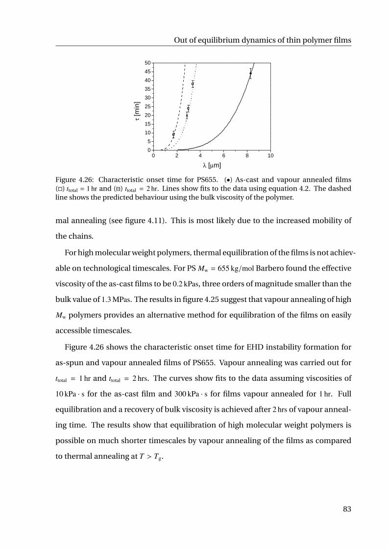
Out of equilibrium dynamics of thin polymer films
0 2 4 6 8 1005
101520253035404550
τ [m
in]
λ [µm]
Figure 4.26: Characteristic onset time for PS655. (•) As-cast and vapour annealed films() ttotal = 1 hr and () ttotal = 2 hr. Lines show fits to the data using equation 4.2. The dashedline shows the predicted behaviour using the bulk viscosity of the polymer.
mal annealing (see figure 4.11). This is most likely due to the increased mobility of
the chains.
For high molecular weight polymers, thermal equilibration of the films is not achiev-
able on technological timescales. For PS Mw = 655 kg/mol Barbero found the effective
viscosity of the as-cast films to be 0.2 kPas, three orders of magnitude smaller than the
bulk value of 1.3 MPas. The results in figure 4.25 suggest that vapour annealing of high
Mw polymers provides an alternative method for equilibration of the films on easily
accessible timescales.
Figure 4.26 shows the characteristic onset time for EHD instability formation for
as-spun and vapour annealed films of PS655. Vapour annealing was carried out for
ttotal = 1 hr and ttotal = 2 hrs. The curves show fits to the data assuming viscosities of
10 kPa · s for the as-cast film and 300 kPa · s for films vapour annealed for 1 hr. Full
equilibration and a recovery of bulk viscosity is achieved after 2 hrs of vapour anneal-
ing time. The results show that equilibration of high molecular weight polymers is
possible on much shorter timescales by vapour annealing of the films as compared
to thermal annealing at T > Tg.
83

Physical phenomena of thin surface layers
4.3 Conclusions
An electric field has been used to weakly perturb the surface of 100 nm thick PS films
cast from various solvents. For films spun from toluene a strong increase in the mo-
bility of the film is observed in as-cast films, corresponding to a reduced effective vis-
cosity of the film. Annealing of the films at T > Tg for sufficiently long times reduces
the mobility of the film and restores the viscosity to that of the bulk polymer.
A similar reduction is seen for films spun from trans-decalin. The measured ef-
fective viscosity for films spun from trans-decalin is less than that of films spun from
toluene. Trans-decalin is a θ−solvent and the viscosity reduction in as-cast films is
seen to depend on the temperature at which the films were spun. Again annealing
of the films above Tg for long times results in a reduction of the film mobility to that
expected from bulk rheology.
The mobility increase observed in the as-cast films can be explained in terms of
non-equilibrium chain conformations caused by the film preparation. Spin-coating
results in a lower entanglement density of the chain compared to a polymer melt at
equilibrium and therefore a reduced effective viscosity. The difference between the
films spun from toluene and from trans-decalin can be explained by the changes in
the chain conformations in the initial solutions and the amount of solvent remaining
in the film at vitrification.
Films spun from chloroform were also seen to have an increased mobility in the
as-cast films as compared to the bulk behaviour. Chloroform is a better solvent for
PS than toluene, implying that the chains in the initial solvent will be more swollen.
However, films spun from chloroform vitrify at higher solvent concentrations. This
suggests that the solvent quality strongly effects the non-equilibrium properties of
spin-cast films.
The experiments show that instabilities in as-cast films have a higher λ than pre-
dicted theoretically, indicating a weak stabilising pressure in the films. These could
84

Out of equilibrium dynamics of thin polymer films
arise from frozen-in normal stresses in the as-cast films. The wavelength is seen to be
greatest for films spun from toluene and smallest for films spun from trans-decalin,
with films spun from trans-decalin at 25 C exhibiting bulk behaviour. This suggests
that spin coating results in an asymmetric deformation of the polymer chains, per-
haps due to solvent evaporation after vitrification. The deformation is dependent on
the conformation of the chain prior to vitrification and the molecular weight of the
polymer.
These frozen-in stresses can be removed by annealing of the films above Tg on
much shorter timescales than those required to restore bulk viscosity. This suggests
that the stresses can relax while the films are still far from equilibrium. Local rear-
rangements of the chains are sufficient to remove the anisotropy responsible for the
residual stress.
The results indicate that the boiling point of the solvent, the film formation time,
the solubility of PS in the solvent and the amount of solvent remaining in the film
on vitrification are all important. No one property can be used to consistently de-
scribe the trends observed in the data. Instead the behaviour observed results from a
combination of all of these parameters.
85


CHAPTER
FIVE
RESIDUAL STRESS IN THIN POLYMER FILMS
In chapter 4 it was shown that the process of spin coating results in the formation
of films with non-equilibrium chain conformations and residual stresses. The wave-
length of the instabilities formed using electrohydrodynamic destabilisation of the
polymer films yields information about the force balance in the film and at the sur-
face, but not the overall magnitude of the stress in the film. The evaluation of resid-
ual stresses is of great importance in the context of technological applications, where
stresses play a role in the adhesive and cohesive properties of the film along with their
stability.
Stresses in thin films are typically measured by coating a cantilever with the ma-
terial of interest and observing the cantilever deflection [123, 124]. The first experi-
ments using this technique were carried out by Stoney in 1909 [125]. Thin metallic
nickel films were deposited by electrolysis onto steel rules. After deposition a deflec-
tion of 3-4 mm was observed in a rule of length×width× thickness = 102×12×0.32 mm.
While widely used to study the stresses in inorganic materials, cantilever deflection
has also been used to investigate the stresses in polymer films. Ree et al. measured
the stresses in spin-coated polyimide films on polished silicon wafers [126]. They
87

Physical phenomena of thin surface layers
used a wafer bending technique, where the deflection was measured using laser light
beams. They found stresses on the order of 11.2−26.8 MPa for as spun films with thick-
nesses of 10 µm. For polystyrene and polyisobutylmethacrylate (PIBM) films blade-
coated onto thin steel cantilevers, Croll found the residual stress to be 4.5 MPa for
PIBM and 14.3 MPa for polystyrene films [127, 128]. This was found to be indepen-
dent of the coating thickness for films of 1 − 100 µm.
Although a well established method, this technique requires that the cantilever is
formed prior to film deposition and measures the stresses in large area films. Micro-
scale cantilevers are used in microelectromechanical systems (MEMS). The fabrica-
tion process of these cantilevers typically involves undercutting the cantilever struc-
ture to release it using a wet or dry etching technique [129]. Such cantilevers have
been used to study the stresses in thin-metallic films sputtered or evaporated onto
their backside.
In this chapter, stresses in 100 nm thick polystyrene films are investigated using
cantilever deflection. The films are spun onto silicon nitride membranes. Focused
ion-beam milling is used to cut cantilevers into the bilayer structures. The deflection
of the cantilevers is monitored by scanning electron microscopy.
Focused ion-beam milling has been used by a number of groups to measure resid-
ual stresses in thin films [130, 131]. Typically a shape is milled out of the material and
the deformation of the structure is monitored using digital image correlation. The de-
formation is used to calculate the residual stresses. This technique allows the stress
in the films to be probed locally and on much smaller length scales than previously
studied in polymer films. It also enables the film to be spin coated, which would not
be possible on pre-formed MEMS cantilevers.
88

Residual stress in thin polymer films
10μm
0.5μ
m
5μm
54˚
SEMFIB
Sample
1
2 3
a b c
Figure 5.1: (a) Membrane sample mounted on SEM stub. (b) A schematic representation ofcantilevers milled using FIB. Numbers and arrows indicate the order in which the edges weremilled and the direction of milling. (c) Orientation of sample with respect to ion and electronbeams.
5.1 Materials and methods
Polystyrene (PS) Mw = 4000 kg mol−1, Mw/Mn = 1.15 (Polymer Standards Service) was
used as obtained without further purification. Films with a thickness of 100 nm were
spun from toluene at a spin speed of 4500 rpm onto 100 nm thick low stress Silicon-
Nitride (SiN) membranes with a 0.5 mm window supported on 200 µm TEM grids (SPI
supplies).
Focused ion beam milling
Focused ion beam (FIB) milling is a commonly used method for the structuring of
surfaces on the micron scale [132]. Here a Carl Zeiss 1540 XB CrossBeam FIB/SEM
system was used to mill cantilevers into the SiN membranes and SiN/PS bilayers. The
substrates were mounted onto SEM stubs using carbon tape, such that the substrates
were free standing and no air was trapped underneath the membrane (figure 5.1a).
Cantilever structures were milled using a 30 keV ion-beam at a current of 100 pA. The
ion-beam was orientated normal to the sample surface. Imaging was carried out us-
ing SEM with a 7 keV electron beam at an angle of 54 to the sample surface. It should
be noted that the FIB was used only to mill the cantilevers and not to image the mem-
branes.
89
Physical phenomena of thin surface layers
Unlike SEM (see chapter 6) FIB is inherently destructive to the sample. The ion
beam is focused into a small spot size and scanned across the sample surface. As the
beam is scanned it removes atoms from the surface, where the number of atoms re-
moved depends on the beam current (dose) and the material being milled. By defin-
ing where the FIB scans, milling can be localised to these areas. Figure 5.1 shows a
schematic representation of the cantilevers that were milled. The approximate di-
mensions, the order in which the edges were milled and the direction of milling are
all indicated. Each shape was milled for 60 s. This was sufficient to mill through the
whole thickness of the SiN/PS bilayer.
5.2 Results and discussion
Figure 5.2a,b shows micrographs of the cantilevers milled in the PS coated silicon ni-
tride membranes. The two cantilevers were cut into different membranes. No imag-
ing of the membranes was carried out using the FIB. Correct positioning of the sam-
ple was achieved using only the SEM. Alignment of the electron and ions beams was
carried out on the supporting silicon wafer, far from the membrane.
Figure 5.2c,d shows images of two cantilevers cut into the same PS coated mem-
brane. The cantilever in figure 5.2c was milled first and imaged using the SEM. The
cantilever in figure 5.2d was then milled and imaged. The first cantilever milled is
seen to deflect upwards and the second downwards. A similar downward deflection
was observed for all subsequent cantilevers milled into the same membrane.
The silicon nitride (SiN) membranes obtained from SPI supplies are manufactured
to have a low intrinsic stress. To check that the deflection observed in figure 5.2a,b,c
was not due to stored stress in the SiN, similar cantilevers were milled into uncoated
membranes. Examples of these are shown in figure 5.3. The initial cantilever milled
is shown in figure 5.3a, while figure 5.3b shows a second cantilever cut into the same
membrane. No deflection is observed in the initial cantilever, while a small down-
90
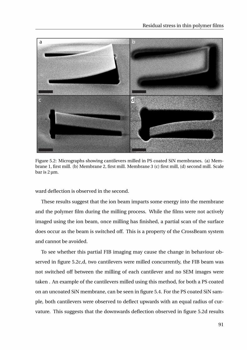
Residual stress in thin polymer films
a b
c d
Figure 5.2: Micrographs showing cantilevers milled in PS coated SiN membranes. (a) Mem-brane 1, first mill. (b) Membrane 2, first mill. Membrane 3 (c) first mill, (d) second mill. Scalebar is 2 µm.
ward deflection is observed in the second.
These results suggest that the ion beam imparts some energy into the membrane
and the polymer film during the milling process. While the films were not actively
imaged using the ion beam, once milling has finished, a partial scan of the surface
does occur as the beam is switched off. This is a property of the CrossBeam system
and cannot be avoided.
To see whether this partial FIB imaging may cause the change in behaviour ob-
served in figure 5.2c,d, two cantilevers were milled concurrently, the FIB beam was
not switched off between the milling of each cantilever and no SEM images were
taken . An example of the cantilevers milled using this method, for both a PS coated
on an uncoated SiN membrane, can be seen in figure 5.4. For the PS coated SiN sam-
ple, both cantilevers were observed to deflect upwards with an equal radius of cur-
vature. This suggests that the downwards deflection observed in figure 5.2d results
91

Physical phenomena of thin surface layers
a b
Figure 5.3: Micrographs showing cantilevers milled in an uncoated SiN membrane. Two can-tilevers were milled one after the another. Imaging was carried out after each cantilever wasmilled. (a) First cantilever. (b) Second cantilever. Scale bar is 2 µm.
a b
c
dd
Figure 5.4: Micrographs showing cantilevers milled in PS coated SiN membrane. Two can-tilevers were milled concurrently with no imaging between mills. (a) Two cantilevers ∼ 20 µmapart. (b,c) Enlargement of the cantilevers shown in (a). (d) Micrograph showing twocantilevers milled concurrently in an uncoated SiN membrane. (a,d) Scale bar is 10 µm.(b,c) Scale bar is 2 µm.
from partial imaging of the sample with the ion-beam.
All images shown here were imaged with the electron beam, after milling had com-
92

Residual stress in thin polymer films
Figure Sample Cut δ (µm) L (µm)1a PS+SiN First 3.06 9.531b PS+SiN First 2.79 9.271c PS+SiN First 1.28 9.371d PS+SiN Second -2.18 8.722a SiN First – 9.372b SiN Second -0.5 9.713a PS+SiN First 2.79 9.273b PS+SiN Second 2.43 8.99
Table 5.1: Deflection and length of the different cantilevers shown in figures 5.2, 5.3 and 5.4.
pleted, at an angle of 54. The deflection and length of the cantilever were measured
using ImageJ software and converted into actual distances. These are shown in table
5.1. It should be noted that while the PS films in figure 5.2a,b and figure 5.4a were
spun on to the membranes and used directly, the PS film in figure 5.2c,d was milled
one month after the film was spun. This may account for the smaller deflection seen
in the initial cantilever.
5.2.1 Cantilever bending
The stresses in the polymer film can be calculated from the deflection of the can-
tilever. The bending of cantilevers due to residual stresses in polymer coatings has
been considered by Corcoran [133]. While only the final equation is required for anal-
ysis of the cantilevers milled here, a summary of the derivation and the assumptions
made are included for completeness.
The method of Corcoran uses plate theory to describe the bending of the can-
tilevers due to the stresses in organic coatings. Plate theory rather than beam theory
(as used by Stoney [125]) is used, since the coating exists in tension in all directions.
The following assumptions are made about the system:
1. The curvature of the deflected cantilever due to the stress in the coating is as-
sumed to be spherical. This is consistent with the small curvatures measured
experimentally. However, due to one end of the cantilever being fixed, the as-
93

Physical phenomena of thin surface layers
sumption will introduce a small systematic error.
2. The PS film adheres perfectly to the membrane. No dewetting of the PS from
the SiN was observed and the film was not seen to delaminate on milling of the
cantilever.
3. The elastic limit is not exceeded in any part of the cantilever.
4. The mechanical properties of the coating and the substrate are isotropic in the
plane of the cantilever. Anisotropy in the film may occur in the plane of the
cantilever due to the spin coating procedure however, the cantilever occupies a
very small area of the film minimising this possibility.
5. The stress is constant through out the thickness of the coating. Chow and Croll
have shown that the stress is independent of thickness [127,134] suggesting that
either there is no variation in the stress over the thickness of the film, or that the
stress distribution takes the same form for any film thickness.
For pure bending of a flat, thin plate, the plate will have a spherical curvature if the
bending moments along the edges are equal i.e. mx = my = m. The curvature is given
by1ρ
=m
D (νs)(5.1)
where ρ is the radius of curvature and ν is Poisson’s ratio. The flexural rigidity
D =Est3
s
12(1 − ν2
s) (5.2)
is the force required to bend a rigid structure to a unit curvature, where E is Young’s
modulus and t is the thickness of the plate. The subscript s refers to the SiN plate.
For a plate fixed at one end the radius of curvature of the bent plate is given by
ρ = L2/2δ, where L is the length of the cantilever and δ is the deflection. Substituting
94

Residual stress in thin polymer films
these into equation 5.1 gives
δ =6mL2 (1 − νs)
Est3s
(5.3)
The deflection due to an applied polymer coating is considered to result from bend-
ing moments applied to the end of the plate, which arise from stresses in the film.
In a bent equilibrium position, the coating is in a state of stress σeq, which exerts an
average force F through the thickness tf of the film. The bending moment per unit
area is given by
m =Mw
=Fw (tf + ts)
2w=σeqtf (tf + ts)
2(5.4)
where w is the width of the plate and M is the total moment applied. Combining
equation 5.3 and equation 5.4 gives the stress in the coating
σeq =δEst3
s
3tfL2 (tf + ts) (1 − νs)(5.5)
The above equation gives the equilibrium stress of the system. If the coating was
instead applied to a rigid substrate, a greater stress would be found. When on a flex-
ible plate the coating compresses, bending the plate. This means that the coating is
shorter than it would be if it were on a rigid plate. This introduces a strain difference
such that
σtot = σeq +εEf
1 − νf(5.6)
where ε = (tf + ts) /2r is the strain difference. The total stress in the film is then found
by combining equations 5.5, 5.6 giving
σtot =Est3
s
6tfρ (ts + tf) (1 − νs)+
Ef (ts + tf)2ρ (1 − νf)
(5.7)
The subscripts s and f refer to the SiN membrane and the PS film respectively.
Young’s modulus of the membrane and PS are taken to be 260 GPa [135] and 3.2 GPa
[86] and poisson’s ratio to be 0.25 [136] and 0.34 [86] respectively. Using equation 5.7,
95

Physical phenomena of thin surface layers
the stress in the as-spun PS film is found to be 211 ± 10 MPa. For the PS films aged
at room temperature for one month the stress is calculated to be 120 ± 6 MPa. This is
in agreement with dewetting experiments, where the residual stresses in the as-cast
films are seen to decrease as the films are aged [106].
The value calculated for the stress in the as spun films is much higher than that
calculated by other groups. Chung et al. monitored the onset of strain-induced wrin-
kling instabilities in PS Mw = 654 kg mol−1 films with thicknesses of 100 − 400 nm and
found the residual stress to be ∼ 30 MPa [137]. Croll carried out cantilever bending
measurements using Dow styron 685 blade coated onto steel rules [128]. The molec-
ular weight of this PS is ∼ 358 kg mol−1 [138]. The stress was found to be 14.3 MPa for
films of up to 18 µm. Neither group saw a change in the measured stress over this
thickness range.
In chapter 4 it was shown that residual stresses, as measured using the onset of
electrohydrodynamic instabilities, increase with increasing Mw of the PS. This is also
seen in the values for the residual stress found in the literature. The PS used for these
experiments had a Mw = 4000 kg mol−1, over six times greater than that used by Chung
et al. This would account for the increased residual stress measured.
Partial imaging of the substrate with the ion beam was found to have an effect on
the deflection of the cantilever beams, for both the uncoated SiN and the PS coated
membrane (see figure 5.2 and figure 5.3). This effect was easily removed by milling
multiple cantilevers concurrently (figure 5.4). The effect of imaging with the electron
beam was not however investigated and while kept to a minimum cannot be avoided
due to the need to align the microscope and observe the cantilevers. Mathrad et al.
have shown that high energy electron irradiation of PS, with doses of up to 8 MeV,
does not change the overall structure of PS films [139]. This indicates that PS is resis-
tant to electron-beam irradiation up to this dose and that the structure should not be
changed by the relatively low beam energies of 7 keV used here.
96

Residual stress in thin polymer films
5.3 Conclusions
The internal stresses stored in spin-cast PS films were measured using a cantilever
deflection technique. Cantilevers were cut into PS coated SiN membranes using a fo-
cused ion beam. On completion of milling the cantilevers were observed to bend up-
wards in the as-spun films. The stress in the PS film was found to be 211 MPa. Subse-
quent cantilevers milled in the same membrane were observed to have a downwards
deflection. This is most likely due to partial imaging with the focused-ion beam on
completion of the milling and was not observed in cantilevers milled concurrently.
The experiments conducted here show that focused ion beam milling of cantilevers
is a promising technique for studying the stored stresses of polymer films. The study
carried out here was a preliminary investigation to check the feasibility of this method.
The dependency of the stresses on the molecular weight of the polymer or the thick-
ness of the film was not investigated. A study of the stresses stored in PS Mw = 655 kg mol−1
would allow a comparison of the residual stresses found using this technique to lit-
erature values and eliminate possible influences of the milling process and electron-
beam imaging on the observed bending of the cantilever. A more accurate determi-
nation of the effect of the ion and electron beams on the polymer film could also be
investigated by flipping the PS/SiN bilayer upside down and imaging/milling it from
the back. If either beam is altering the stresses in the polymer film then a smaller
deflection should be observed for a cantilever milled in this configuration. This tech-
nique could also be used to measure the stresses in much thinner films than those
that have been previously been studied.
In agreement with literature, the stresses in the polymer film were observed to de-
crease for films aged at room temperature. Since the films are aged at T < Tg full
equilibration of the films did not occur. As shown in chapter 4 equilibration through
thermal annealing for high molecular weight polymers is not achievable on experi-
mentally accessible timescales. Experiments on vapour annealed films, would allow
97

Physical phenomena of thin surface layers
cantilevers to be milled into fully equilibrated films. It is expected that a much smaller
deflection in these films will be seen due to full relaxation and entanglement of the
polymer chains.
A further application of focused ion beam milling would be to locally map out the
stresses in spin-cast films, by spin coating of the polymer film onto a multi-frame
array of membrane windows. By milling cantilevers into the different windows the
stresses could be mapped out over centimetre areas.
98

CHAPTER
SIX
PALLADIUM DOPED POLYMER PRECURSORS FOR
MAGNETIC CERAMICS
Organometallic polymers containing transition metals in the backbone have attracted
considerable attention [140–143] since the discovery of ferrocene nearly sixty years
ago [144]. These materials have desirable properties [145] and applications as cata-
lysts [146], sensors [147] and ceramic precursors [142]. Their unique processing char-
acteristics allow for the possible fabrication of complex and nanostructured shapes
[148] with a variety of magnetic properties [8].
One organometallic system which has received a large amount of interest over re-
cent years is the metallocene-based polyferrocenylsilane (PFS) [149, 150]. PFS is an
iron and silicon containing polymer, which when pyrolysed yields magnetisable ce-
ramics due to the presence of clusters containing iron [151]. The size and type of
these clusters can be controlled by adjusting the pyrolysis conditions. At lower py-
rolysis temperatures (around 600 C) the formation of ceramics containing small su-
perparamagnetic iron nanoclusters in an amorphous ferromagnetic carbon/silicon
carbide matrix [152] is observed. Increasing the temperature of pyrolysis to around
1000 C, leads to an increase in the cluster size and the generation of ferromagnetic
99

Physical phenomena of thin surface layers
ceramics containing α−Fe crystallites.
Cross-linking of precursors allows for higher ceramic yields, magnetic properties
which are tunable and the ability to produce molded ceramics due to high shape re-
tention [8,153,154]. For example, MacLachlan et al. [8] have shown that a cross-linked
network of spirocyclic [1]silaferrocenophane can be used to form ceramics whose
properties at room temperature can be tuned between superparamagnetic and fer-
romagnetic states, by controlling the pyrolysis conditions. These polymers can be
shaped on the macroscopic scale or patterned on the micron-scale prior to pyrolysis,
with the ceramic products retaining the patterned shape with high-fidelity. Higher
ceramatisation yields and increased iron content are also seen from hyperbranched
polyferrocenylsilanes [155]. These produce mesoporous ferromagnetic materials, with
a negligible hysteresis loss when pyrolysed at high temperatures under argon, due to
the formation of iron silicides. These materials have potential applications for data
storage and electromagnetic shielding [156]. PFS has also been used as a precursor
to form microspheres with low polydispersity [154], allowing for the synthesis of mi-
crospheres with tailorable redox, semiconductive and magnetic properties [157].
Another interesting application of metal containing polymers is their use as pre-
cursors for the synthesis of bimetallic nanoparticles. This has been demonstrated
for iron-platinum (FePt) nanoparticles [158] formed from the pyrolysis of bimetallic
metallopolynne precursors. Pyrolysis of PFS precursors with pendant cobalt clusters
and polycarbosilanes with pendant nickel clusters have been shown to yield cobalt-
iron [159] and nickel or nickel silicide nanoparticles respectively [160].
Variation in the pyrolysis conditions results in changes to the nanoparticle size,
distribution and composition. Thin films containing CoFe nanoparticles were shown
to exhibit superparamagnetic behaviour, with ferromagnetic behaviour being ob-
served for pyrolysis at higher temperatures. This is attributed to a stabilisation of
the nanoparticle magnetisation on the time scale of the hysteresis measurement due
to the increased size of the nanoparticles which form at higher temperatures. Pyroly-
100

Palladium doped polymer precursors for magnetic ceramics
sis of the nickel containing polycarbosilanes yielded ceramics embedded with nickel
particles or nickel silicides depending on the pyrolysis conditions, with both super-
paramagnetic and ferromagnetic behaviour being observed.
While this shows that bimetallic precursors can be used to synthesis nanoparticles
with desirable properties, these precursors can be hard to synthesise as they require
the controlled incorporation of different metals into the macromolecular architec-
ture and ancillary ligands which do not interfere in the nanoparticle formation. This
chapter focusses on the formation of ceramic films containing FePd nanoparticles
from polyferrocenylethylmethylsilane (PFEMS) using the physicochemical methods
of evaporation, reduction and thermal breakdown. The incorporation of Pd into poly-
mer precursors is desirable due to the unique properties of Pd and the magnetic
properties of FePd alloys [161]. These are of paramount technological relevance due
to the large saturation magnetisation and magneto-crystalline anisotropy (hard mag-
netic behaviour), persistent even in FePd nanoparticles larger than 8 nm [162, 163],
rendering them suitable for ultra-high density magnetic storage [164].
101

Physical phenomena of thin surface layers
FeH
SinBu
Me Et
n
Figure 6.1: Molecular structure of PFEMS.
6.1 Materials and methods
The PFEMS homopolymer was prepared by living anionic ring opening polymerisa-
tion of ethylmethylsila[1]ferrocenophane as described in [165]. Figure 6.1 shows the
molecular structure of the polymer. The molecular weight and polydispersity index of
the material used in this study were 22.5 kg mol−1 and 1.01 respectively, as determined
by Gel Permeation Chromatography (GPC). GPC was carried out on a Viscotek GPC-
max chromatograph equipped with a triple detector array. A flow rate of 1.0 ml min−1
was used with THF as the eluent1. Palladium(II)-acetylacetonate (Pd(acac)2) 99% pu-
rity was obtained from Sigma-Aldrich and used without modification.
The addition of Pd to the PFEMS was carried out using two different methods;
as nanoparticles through sublimation of palladium-acetylacetonate (Pd(acac)2) or
through direct mixing of the Pd(acac)2 into the PFEMS prior to pyrolysis of the films.
The pyrolysis scheme is shown in table 6.1. Three sets of films were made: pure
PFEMS films (precursor 1), PFEMS films containing Pd nanoparticles (precursor 2)
and PFEMS films containing Pd(acac)2 (precursor 3). Pure PFEMS films were formed
by drop-coating PFEMS-toluene solutions onto naturally oxidised Si(100) wafer sub-
strates obtained from Silicon Materials. The dry films were subsequently annealed in
a vacuum oven at 60 C for 24 hrs. For PFEMS films containing Pd(acac)2, the Pd(acac)2
was mixed into the PFEMS-toluene solutions prior to drop coating with a w/w ratio
of 1:4 Pd(acac)2:PFEMS. The Pd nanoparticle deposition was carried out using the
1Polymerisation of PFEMS and GPC measurements were carried out by J. Gwyther at the Universityof Bristol.
102

Palladium doped polymer precursors for magnetic ceramics
a b
Figure 6.2: TEM micrographs of a PFEMS film (a) before and (b) after Pd nanoparticle depo-sition. Scale bar is 200 nm.
method described in [166]. The PFEMS films were placed in a crystallisation dish,
with ∼ 13 mg of Pd(acac)2. The crystallisation dish was filled with nitrogen, sealed
and placed in a box oven, which was pre-heated at 170 C, for 1 hr. The Pd(acac)2, sub-
limes and Pd nanoparticles form through the thermal decomposition of PD(acac)2 to
metallic Pd. TEM images before and after this exposure are shown in figure 6.2.
Pyrolysis was initially carried out in a tube furnace under nitrogen at 600 C and
1000 C for 3 hrs with a heating rate of 15 C min−1. The results from these experiments
however, indicated that the nitrogen atmosphere had some oxygen impurities. As a
result pyrolysis was also carried out under argon at 1000 C. Substrates were weighed
Ceramic Name Precursor Pyrolysis Temperature (C) Pyrolysis Atmosphere1aN 1 600 N2
1bN 1 1000 N2
1bA 1 1000 Ar2aN 2 600 N2
2bN 2 1000 N2
2bA 2 1000 Ar3aN 3 600 N2
3bN 3 1000 N2
3bA 3 1000 Ar
Table 6.1: Pyrolysis scheme for the different ceramics.
103

Physical phenomena of thin surface layers
SQUID
sampledetectioncoils
magnet
sample motion
liquidhelium
air lock
Figure 6.3: Schematic diagram of a SQUID magnetometer showing the basic setup (imageadapted from [167]).
before and after film deposition and samples were weighed before and after pyrolysis.
SQUIDs
The magnetic properties of the films and ceramics were measured at room tempera-
ture and 5 K using a Quantum Design MPMS Superconducting Quantum Interference
Device (SQUID) magnetometer.
Superconducting quantum interference devices (SQUID) are highly sensitive de-
tectors of magnetic flux, which can measure weak magnetic fields as low as 10−17 T.
They are able to measure any quantity that can be converted to a flux, such as mag-
netic field, current, voltage, displacement and magnetic susceptibility, making them
very versatile. As a result, the applications of SQUIDs are wide ranging, from the de-
tection of tiny magnetic fields produced by the brain [168], to the detection of gravity
waves [169]. Here a SQUID was used to analyse the magnetic properties of the pre-
cursor and ceramic films.
The basic phenomena governing the operation of SQUID devices are flux quanti-
sation in superconducting loops and the Josephson effect. A detailed description of
104

Palladium doped polymer precursors for magnetic ceramics
the theory behind SQUIDs can be found in [170]. The system contains a homogenous
superconducting magnet as shown in figure 6.3, to create a uniform field over the en-
tire region in which the sample is measured. A dc-field is applied across the sample
to induce a permanent magnetic moment. This field is kept fixed, while the sample
is moved into a set of superconducting detection coils. As the sample passes through
the coil, the magnetic moment of the sample induces a current in the detection coils.
The current passes through an inductance loop generating a magnetic flux which is
fed into a SQUID. The output voltage is dependent on the position of the sample and
the applied field. By varying the applied field, the hysteresis behaviour of the sample
can be measured.
EDX Analysis
Energy dispersive X-ray (EDX) elemental analysis was performed to look at the atomic
composition of the ceramics, using an FEI Philips XL30 sFEG with an EDX detector.
Measurements were carried out at 20 kV, 15 kV and 12 kV at a working distance of
5 mm. Three different areas were measured for each sample and averaged to take into
account composition variations across the films.
During EDX analysis, the sample is placed inside a scanning electron microscope
and bombarded with a beam of electrons2. These electrons collide with electrons
within the sample, knocking them out of their orbits. The empty positions are then
filled with electrons from outer energy shells. The energy difference between these
two shells is emitted as an X-ray. The energy of the X-ray is dependent on the element
being bombarded and the difference in energy between the shells that the electron
has moved from and to. The X-rays are detected using an energy dispersive spec-
trometer. The energy and number of X-rays detected can be used to find the atomic
composition and the weight percent of each element in the sample.
2EDX analysis is an integrated function of a scanning electron microscope. It cannot be operatedindependently.
105

Physical phenomena of thin surface layers
X-ray diffraction
The bulk composition and crystalline structure of the precursors and ceramics were
investigated using X-ray diffraction (XRD). This technique is based on the construc-
tive interference of monochromatic X-rays with a crystalline sample and is widely
used for the identification of unknown crystalline materials. An X-ray diffractome-
ter consists of three different elements: an X-ray tube, a sample holder and an X-
ray detector. The X-rays are generated by a cathode ray tube, filtered to produce
monochromatic radiation, collimated to increase intensity and directed towards the
sample. Interaction of the incident radiation with the sample produces construc-
tive interference when the Bragg condition is satisfied i.e. nλ = 2d sin θ, where λ is
the wavelength of the radiation and d is the lattice spacing of the crystalline sample.
When the crystals are randomly orientated, scanning over all 2θ angles allows for all
possible diffraction directions of the lattice to be obtained. For a detailed discussion
of crystallography and X-ray diffraction see [171].
X-ray diffractograms were obtained using Philips PW1820 and PW3020 X-ray gen-
erators with a CuKα (λ = 1.54178 Å) radiation source. The samples were mounted
on an amorphous silicon wafer. The angle was varied from 2 to 75 in steps of 0.05
with 2.5 s per step. The peaks were identified by comparison with data files from the
PCPDFWIN crystallographic database.
Microscopy
Image analysis was carried out using a Leo variable pressure Scanning Electron Mi-
croscope (SEM) and a Philips Technai 20 Transmission Electron Microscope (TEM).
The samples were formed directly on the TEM grids, by dip coating them into the
PFEMS-toluene solutions. The use of TEM for imaging is discussed in chapter 7. For
imaging of the PFEMS-Pd films, no staining was carried out.
In scanning electron microscopy (SEM) an electron beam is focussed into a small
spot size and scanned over the surface of a sample, releasing secondary electrons.
106

Palladium doped polymer precursors for magnetic ceramics
a b c
Figure 6.4: SEM micrographs of ceramics (a) 1bA, (b) 2bA and (c) 3bA. Scale bar is 1 µm.
These are recorded using a secondary electron detector. Only secondary electrons
close to the surface (< 10 nm) can exit the sample and be detected, due to the rela-
tively low energy of these electrons. By correlating the number of electrons with the
position of the scan a topographical image of the sample can be generated, where
the intensity of the pixel corresponds to the number of electrons detected at that po-
sition.
6.2 Results
Pyrolysis of the PFEMS films without the addition of Pd under nitrogen, 1aN and 1bN,
resulted in a red coloured ceramic. Figure 6.4 shows examples of the film morphology
for ceramics pyrolysed under argon. Similar morphologies were seen for all ceramics.
Energy Dispersive X-ray (EDX) analysis was used to investigate the chemical com-
position of the polymer and the ceramics. Four elements were detected by EDX in the
PFEMS precursor film: carbon (C), silicon (Si), iron (Fe) and oxygen (O). For ceramics
1aN and 1bN three elements were found: O, Si and Fe. Si and Fe come from the poly-
mer precursor. Oxygen has been found in the ceramics, even though pyrolysis was
conducted in a sealed quartz tube under nitrogen. No C was detected in samples py-
rolysed under nitrogen, but was seen for samples pyrolysed under argon (table 6.2).
107

Physical phenomena of thin surface layers
Element (wt.%) 1bA 2bA 3bAC 28.61 23.70 22.26(13.83)[8.24]O 39.46 34.47 34.64(34.83)[33.63]Si 11.96 13.91 9.52(11.44)[13.00]Fe 19.97 18.88 21.22(27.84)[33.86]Pd – 9.004 12.36(12.06)[11.18]
Table 6.2: Composition of ceramics, pyrolysed under argon, estimated using EDX analysis.Values indicate the weight percentage of each element, measured with a beam energy of20 keV (15keV) and [12keV].
The literature shows that oxygen is often found in ceramics prepared using the
precursor method [155]. Oxygenic compounds may stem from moisture absorbed
by the polymers prior to pyrolysis and/or from post-oxidation of the samples during
handling and storage. They may also arise from impurities in the nitrogen used to
purge the furnace prior to and during pyrolysis. Table 6.2 shows the composition of
films pyrolysed under argon in terms of the weight percent of each element at a beam
energy of 20 keV.
The EDX data for ceramics pyrolysed under argon are shown in table 6.2. Example
traces for ceramics 1aN and 2aN are shown in figure 6.5. The results are representa-
tive of all the ceramics. Analysis of ceramics pyrolysed from precursors 2 and 3 indi-
cates the presence of Pd (figure 6.5b). For samples 2aN, 2bN and 2bA, Pd nanoparti-
cles were incorporated into the films through sublimation of Pd(acac)2. TEM images
before and after this exposure are presented in figure 6.2 and show the addition of Pd
nanoparticles with an average diameter of 6 nm.
When probing the samples with electron beams of different energies, the probing
depth of the sample is altered, with lower beam energies having a smaller penetra-
tion depth [172]. For films pyrolysed under argon, a dramatic decrease in the carbon
content is seen as the beam energy is decreased. Data for sample 3bA are shown in
table 6.2. The data suggest that there is less carbon at the surface than in the bulk,
which may be a result of oxidation of the surface, perhaps due to the adsorption of
oxygen on the film prior to loading. The Pd content of all Pd containing samples does
108

Palladium doped polymer precursors for magnetic ceramics
0 1 2 3 4 5 6 7 8
Energy (keV)0 2 4 6 8 10
Energy (keV)
a b
O
O
Si Si
Fe
Fe
Fe
FePd
Figure 6.5: EDX analysis traces for samples (a) 1aN and (b) 2aN.
not change with probe depth, while the Fe content increases with decreasing probe
depth, suggesting that Fe is more abundant at the surface of the films. Similar be-
haviour was observed for all Pd containing ceramics and is consistent with previous
studies [173]
X-Ray Diffraction (XRD) analysis was carried out to investigate the bulk compo-
sition and crystal structure of the ceramic products. The XRD patterns are shown
in figure 6.6. All samples had a strong reflection peak at 69.13 arising from the Si
wafer used as the substrate. This peak was used to align the individual scans and to
determine the accurate position of the other peaks; it is not shown in figure 6.6 for
clarity. XRD characterisation of samples 1bA, 2bA and 3bA was carried out on a dif-
ferent generator to that used for the other samples. Harmonic peaks are observed
from the Si(400) peak when using this generator due to the absence of a filter. These
three spectra are plotted together along with the spectra of the silicon substrate for
clarity (figure 6.6d). The PFEMS polymer precursor 1 is amorphous, exhibiting no
sharp reflection peaks, but a diffuse halo in the 2θ angle region centred around 13
between 10 to 18. The diffuse halo is also seen for the Pd containing precursor films
2 and 3 along with additional peaks, which come from the Pd. Comparison of precur-
sor films 1 and 3, show that the Pd(acac)2 has strong peaks at 2θ = 11.85 d = 7.47 Å,
109

Physical phenomena of thin surface layers
10 20 30 40 50 600
20
40
60
80
2θ(degrees)
10 20 30 40 50 600
20
40
60
80
10 20 30 40 50 6010 20 30 40 50 60
2θ (degrees)
10 20 30 40 50 600
20
40
60
80
2θ (degrees)
a b
c
Precursor 1Precursor 2
1aN
1bN
2aN
2bN
Precursor 3
3aN
3bN
10 20 30 40 50 600
20
40
60
80
2θ/degrees
3bA
2bA
1bA
Silicon
d
Figure 6.6: XRD data (a) PFEMS precursor and ceramic films. (b) PFEMS precursor and ce-ramic films containing Pd nanoparticles. (c) PFEMS precursor and ceramic films containingPd(acac)2. (d) Ceramic films pyrolysed under argon.
12.66(6.99 Å), 16.39(5.41 Å), 17.90(4.96 Å), 26.08 (3.42 Å) and 28.45(3.14 Å). These
correspond very closely to those found for powdered Pd(acac)2 at by Cominos et
al. [174].
The ceramic products of 1, 2 and 3 show diffraction patterns with numerous Bragg
reflections, indicating that the ceramics contain a number of crystalline species. The
Scherrer equation [175] can be used to estimate the size of the crystals present in the
samples. The equation is given by
τ =Kλ
β cos θ(6.1)
where K is the shape factor, λ is the X-ray wavelength, β is the line broadening of the
110

Palladium doped polymer precursors for magnetic ceramics
peak at full width half maximum and θ is the Bragg angle. Using equation 6.1, the size
of the crystals is estimated to be between 18−45 nm. This is smaller than the size of the
crystals seen in the SEM images (figure 6.4), which are on the order of 100 − 200 nm in
size, suggesting that the ceramic crystalline structures, as seen by SEM, are not pure
in composition. Instead clusters of different species coexist.
Data files from the crystallographic database were used to identify the peaks ob-
served in the XRD spectra (figure 6.6). The results are summarised in table 6.3. All the
ceramics show reflection peaks at 2θ ' 35.6 (d = 2.52 Å) corresponding to ferrimag-
netic Fe3O4 and γ−Fe2O3. Sample 1bA exhibits an additional higher order reflection
peak of γ−Fe2O3 at 57.24 (1.61 Å). This was not detected for the other ceramic sam-
ples, probably due to imperfect packing of the crystals. The reflection peaks associ-
ated with α−Fe2O3 at 33.15 (2.70 Å) and 35.61 (2.52 Å) are seen for all ceramics apart
from 1aN and 2aN. The second order reflection observed in the XRD spectra from
α−Fe2O3 suggests that Fe2O3 exists mainly in the α form. The peaks associated with
reflections of α−Fe metal are only seen in the spectra for 1bA, where a very weak peak
is observed. Thus, the majority of iron species exist in oxide form. The stronger peaks
are observed for the ceramics pyrolysed at 1000 C under argon (1bA, 2bA, 3bA).
For ceramics pyrolysed under nitrogen, carbon is only observed in the spectra of
3aN. It is present in all samples pyrolysed under argon. This strongly suggests im-
purities in the nitrogen atmosphere used for pyrolysis lead to oxidative degradation.
The reflection peaks of SiO2 and SiC are weak and broad. This is most likely due to
the majority of silicon and carbon species existing in the amorphous state.
Pd exists as pure Pd (3aN), PdSi (2aN) and Pd2Si. The peaks of Pd2Si are observed at
38.26 (2.35 Å) for all Pd containing samples apart from 2aN. Ceramics 2bN and 3bA
also show higher order reflections peaks for Pd2Si at 41.53 (2.17 Å), 42.22 (2.14 Å) and
48.76 (1.87 Å). The peaks are most prominent in ceramics pyrolysed under argon.
Pd and FePd alloys exhibit similar reflection peaks. Bryden et al. [176] have shown
that pure Pd exhibits a peak at ∼ 40. They synthesised FePd alloys and showed that
111

Physical phenomena of thin surface layers
Crystal
1aN1b
N1b
A2aN
2bN
2bA
3aN3b
N3b
AFile
α–Fe
43.4(2.05)31-0619
Fe3 O
435.62(2.52)
35.53(2.53)35.65(2.52)
35.51(2.53)35.61(2.52)
35.62(2.52)35.63(2.52)
35.63(2.52)35.55(2.53)
19-0629
α–Fe
2 O3
32.93(2.72)33.08(2.71)
33.16(2.70)33.08(2.71)
33.08(2.71)33.08(2.71)
33.08(2.71)33-0664
35.53(2.53)35.65(2.52)
35.61(2.52)35.62(2.52)
35.63(2.52)35.63(2.52)
35.55(2.53)
54.08(1.7)54.13(1.69)
γ–Fe2 O
335.62(2.52)
35.53(2.53)35.65(2.52)
35.51(2.53)35.61(2.52)
35.62(2.52)35.63(2.52)
35.63(2.52)35.55(2.53)
39-1346
57.24(1.61)
SiO2
30.33(2.95)30.49(2.93)
30.28(2.95)30.28(2.95)
30.13(2.97)30.08(2.71)
72-2310
29.14(3.06)29.03(3.08)
72-1601
C26.64(3.35)
26.65(3.35)26.83(3.32)
26.52(3.39)75-2078
S iC35.61(2.52)
35.62(2.52)35.63(2.52)
35.63(2.52)35.55(2.53)
75-1541
38.25(2.35)38.56(2.33)
38.60(2.33)38.39(2.34)
38.46(2.34)
Pd
––
–40.5(2.23)
7440-05-3
Pd
Fe–
––
40.16(2.25)40.06(2.25)
40.01(2.25)[176,177]
––
–46.68(1.95)
46.74(1.94)46.60(1.95)
Pd
Si–
––
29.03(3.08)07-0127
Pd
2 Si–
––
38.25(2.35)38.56(2.35)
38.60(2.33)38.39(2.34)
38.46(2.34)06-0559
––
–41.53(2.17)
42.31(2.14)41.94(2.15)
––
–42.22(2.14)
48.24(1.89)
––
–48.76(1.87)
T able
6.3:Nan
ocrystals
inth
eceram
icsas
iden
tified
by
XR
Dan
alysis
112
Palladium doped polymer precursors for magnetic ceramics
as the volume fraction of Fe in the alloys increases, secondary reflections at ∼ 46
start to appear and grow stronger. A small shift in the position of FePd peaks rela-
tive to Pd peaks has also been reported [177]. Ceramic 3bN exhibits a small peak at
40.5(2.23 Å), corresponding to a reflection peak of Pd, no higher order reflections are
seen. Ceramics 2bA and 3bA have a reflection peak at 40.01(2.25 Å), which is lower
than that seen in 3bN and have higher order reflections at 46.6(1.95 Å) suggesting
that the reflections come from FePd. This peak increases in magnitude from sample
2bA to 3bA, which is indicative of an increase in iron content in the FePd alloys [176].
SQUID magnetometry was used to investigate the magnetic behaviour of the films
in a magnetic field at room temperature. The ceramics films fabricated from polymer
precursors with the addition of Pd nanoparticles and Pd(acac)2 and pyrolysed at dif-
ferent temperatures and under different atmospheres displayed different magnetic
properties. The magnetisation curves are shown in figure 6.7. The precursor films 1,
2 and 3 all displayed paramagnetic behaviour at room temperature. The PFEMS pre-
cursor film (precursor 1) had a susceptibility of 11.28±0.08×10⁻⁶ emu/g 3. The addition
of Pd in nanoparticle form to the PFEMS increased the susceptibility four-fold. Films
made from precursor 3, where the Pd(acac)2 had been mixed directly with the poly-
mer, had a susceptibility nearly ten times greater than that of precursor 1 (table 6.4).
The pyrolysed samples were all found to display ferromagnetic behaviour (figure
6.7). The saturation magnetisation Ms, remanent magnetisation Mr and coercivity Hc
for the samples are given in table 6.4. Films pyrolysed from precursor 1 had the low-
est coercivity. This increased as Pd was added first in nanoparticle form (samples
pyrolysed from precursor 2) and then directly as Pd(acac)2 (samples pyrolysed from
precursor 3). The highest coercivity was seen for samples pyrolysed under argon. In-
creasing the pyrolysis temperature to 1000 C resulted in an increase in the coercivity
for all the ceramics. The coercivity of samples 1bN and 2bN are comparable, whilst
sample 3bN had a coercivity four times greater. For samples pyrolysed under argon,
3Units of mass magnetisation: 1 emu/g = 4π × 10−7 Am2/kg
113

Physical phenomena of thin surface layers
a
b
c
d
e
f
-40000 -20000 0 20000 40000
-12
-8
-4
0
4
8
12
Mas
s M
agne
tisat
ion
(em
u/g)
Field (Oe)
-40000 -20000 0 20000 40000
-12
-8
-4
0
4
8
12
Mas
s M
agne
tisat
ion
(em
u/g)
Field (Oe)
-40000 -20000 0 20000 40000
-12
-8
-4
0
4
8
12
Mas
s M
agne
tisat
ion
(em
u/g)
Field (Oe)
-2000 -1000 0 1000 2000
-8
-4
0
4
8
Mas
s M
agne
tisat
ion
(em
u/g)
Field (Oe)
-2000 -1000 0 1000 2000
-12
-8
-4
0
4
8
12
Mas
s M
agne
tisat
ion
(em
u/g)
Field (Oe)
-2000 -1000 0 1000 2000
-12
-8
-4
0
4
8
12
Mas
s M
agne
tisat
ion
(em
u/g)
Field (Oe)
Figure 6.7: SQUID magnetisation curves at room temperature. (a) Precursor 1 and ceramics.(b) Precursor 2 and ceramics. (c) Precursor 3 and ceramics. (d), (e), (f) Magnification of (a),(b) and (c) respectively. (•) Precursor films. () Ceramics pyrolysed at 600C under nitrogen,(N) at 1000C under nitrogen and () at 1000C under argon.
the coercivity of ceramics 1bA and 2bA was the same, with a small increase being
observed for 3bA.
The remanent magnetisation measured for the ceramic films from the SQUID mag-
114

Palladium doped polymer precursors for magnetic ceramics
Sample χρ (×10−6 emu/g) Ms (emu/g) Mr (emu/g) Hc (Oe)Precursor 1 11.28 ± 0.08 – – –Precursor 2 40.04 ± 0.4 – – –Precursor 3 101.6 ± 0.3 – – –
1aN – 4.3 ± 0.1 0.031 ± 0.005 9.7 ± 0.52aN – 6.96 ± 0.2 0.17 ± 0.01 64 ± 23aN – 5.68 ± 0.2 0.20 ± 0.01 80 ± 51bN – 7.16 ± 0.07 1.16 ± 0.01 77 ± 52bN – 6.95 ± 0.3 1.26 ± 0.02 87 ± 23bN – 9.12 ± 0.1 3.99 ± 0.02 338 ± 201bA – 8.18 ± 0.2 3.48 ± 0.01 257 ± 52bA – 12.2 ± 0.2 5.74 ± 0.01 256 ± 103bA – 12.0 ± 0.2 5.30 ± 0.01 298 ± 10
Table 6.4: Magnetic properties of the precursors and ceramics. Susceptibility χρ, saturationmagnetisation Ms, remanent magnetisation Mr and coercivity Hc.
netisation curves at RT are shown in figure 6.8b. The remanence increases with in-
creasing pyrolysis temperature and from films pyrolysed under N2 to those pyrolysed
under Ar (table 6.4). An increase in the remanence is seen on addition of Pd, with
films pyrolysed from precursor 3 displaying the largest remanent magnetisation.
The remanent magnetisation for precursor 1 pyrolysed at 600 C is 0.031±0.005 emu/g.
This increased five-fold for Pd containing films. There was only a small difference be-
tween the Pd containing ceramics 2aN and 3aN formed using the two different Pd
deposition methods. For films pyrolysed at 1000 C under N2 the remanent magneti-
sation for 1bN and 2bN was comparable and strongly increased for 3bN. For ceramics
pyrolysed under argon from precursor 1, the remanence was increased three fold as
compared to those pyrolysed under N2. The remanence for films 2bA and 3bA also
strongly increased.
The change in saturation magnetisation for the different ceramics is shown in fig-
ure 6.8c. A strong enhancement is seen for films containing Pd and from samples
pyrolysed under argon. Ceramics 2bA and 3bA had saturation magnetisations of
12.2 ± 0.2 emu/g and 12.0 ± 0.2 emu/g respectively. This is nearly three times higher
than the saturation magnetisation of ceramic 1aN of 4.3 ± 0.1 emu/g.
115

Physical phenomena of thin surface layers
1 2 30
40
80
120
160
200
240
280
320
360
400
N2 600oC N2 1000oC Ar 1000oC
Coe
rciv
ity (O
e)
Precursor1 2 3
0
1
2
3
4
5
6
N2 600oC N2 1000oC Ar 1000oC
Rem
nant
Mag
netis
atio
n (e
mu/
g)Precursor
1 2 3
4
5
6
7
8
9
10
11
12
13
Sat
urat
ion
Mag
netis
atio
n (e
mu/
g)
Precursor
N2 600oC N2 1000oC Ar 1000oC
a b c
Rem
anen
t
Figure 6.8: (a) Coercivity, (b) remanent magnetisation and (c) saturation magnetisation fromthe SQUID data for samples measured at room temperature.
6.3 Discussion
The pure PFEMS polymer and Pd doped polymer precursors are shown to be para-
magnetic, with susceptibilities ranging from 11 − 102 × 10−6 emu/g. This appears to
be the first time that such data on the paramagnetic behaviour of PFEMS have been
reported. This behaviour may arise from small amounts of oxidation of the Fe(II) cen-
tres to the Fe(III) state. Pd is a strong paramagnet with a susceptibility of 567.4 × 10⁻⁶ emu/g
at room temperature. The increase in susceptibility of the precursor on addition of
Pd, is most likely a result of the Pd acting as additional localised dipoles in the precur-
sor. When pyrolysed under nitrogen, the pure PFEMS film forms a ceramic predom-
inantly containing Fe oxides, in particular Fe3O4 or γ−Fe2O3. Both these oxides are
ferrimagnetic materials. Only the main XRD peaks are seen here (figure 6.6), which
are similar and therefore are hard to distinguish from one another. While the X-ray
results do not show unambiguous stoichiometry, in some cases the EDX results can
be used to deduce whether Fe3O4 or γ−Fe2O3 is most prevalent in the sample. Anal-
ysis of the data for samples 1aN and 2aN suggests that the peak at 35.62 most likely
comes from Fe3O4 due to the amount of oxygen available to form Fe-oxides. However,
the presence of γ−Fe2O3 cannot be ruled out and it is likely that a mixture of the two
oxides is present in the ceramics.
The EDX analysis of the ceramics indicates that oxidation of the samples occurs
either during or after pyrolysis. Analysis of sample 1bA shows that elemental iron
116

Palladium doped polymer precursors for magnetic ceramics
-1000 -500 0 500 1000
-10
-5
0
5
10
Mas
s M
agne
tisat
ion
(em
u/g)
Field (Oe)-1000 -500 0 500 1000
-10
-5
0
5
10
M
ass
Mag
netis
atio
n (e
mu/
g)
Field (Oe)
a b
Figure 6.9: SQUID magnetisation curves at 5K. (a) Ceramics (H) 1bA and () 2bA. (b) Ceramics(N) 1bN and (•) 2bN. Dashed lines are a guide for the eye indicating the exchange bias.
formed during pyrolysis, suggesting that Fe forms initially and is then oxidised. The
lack of carbon in the ceramics pyrolysed under nitrogen, suggests that for these sam-
ples, oxidation occurs both during and after pyrolysis, perhaps as a result of a con-
taminated atmosphere. For the ceramics pyrolysed under argon, the results indicate
that oxidation of the Fe predominantly occurs post-pyrolysis. It should be noted that
while the ceramics were allowed to cool to room temperature in the furnace under the
nitrogen and argon atmospheres, they were not encapsulated. Once removed from
the furnace the ceramics immediately came into contact with the air in the room.
The presence of the antiferromagnetic α−Fe2O3 (hematite) phase is confirmed by
X-ray analysis in the majority of the samples and by magnetometry results. An ex-
change bias effect [178] is observed in pure PFEMS (1bN and 1bA) and in Pd nanopar-
ticle doped ceramics (2bN and 2bA) pyrolysed at 1000 C upon field cooling of the
samples with a 1 T applied field to 5 K, as shown in figure 6.9. This is below the Morin
transition temperature4 of 250 K [179]. The resulting exchange bias fields were −90 Oe
5 for 1bA and 2bA, −60 Oe for 1bN and −40 Oe for 2bN. These results indicate the pres-
ence of core-shell clusters of ferromagnetic Fe (1bA) and ferrimagnetic Fe-oxides sur-
4A magnetic phase transition temperature in α−Fe2O3.5Units of applied magnetic field: 1 Oe = 103/4πAm−1
117

Physical phenomena of thin surface layers
rounded by a shell of α−Fe2O3, similar to those seen by Crisan et al. [180]. No such ef-
fect was observed for the ceramics arising from PFEMS and Pd(acac)2 (3bN and 3bA).
The exchange bias effect, which arises from the pinning of the ferromagnetic domain
by the adjuncted antiferromagnetic surface, results not only in a shift of the hystere-
sis known as the exchange bias field, but can also significantly alter the coercivity of
the ferromagnet/ferrimagnet by acting as a pinning site of the domains upon reversal
of the magnetisation. The absence of this effect in the ceramics pyrolysed from the
Pd(acac)2 precursor, indicates the absence of physical contact between hematite and
the FePd clusters.
The magnetic properties of Fe-oxides are reported to be highly dependent on crys-
tallinity, particle size, sample shape and purity [181]. The saturation and remanent
magnetisation of nanocomposites of Fe2O3 and Fe3O4 have been widely studied [180–
183] and were found to be significantly lower than the values reported for bulk ma-
terial [184, 185]. The difference is attributed to the small particle size effect [186] and
the inclusion of non-magnetic nanocomposites within the matrix of other materi-
als, which reduces mass magnetisation. For γ−Fe2O3 nanoparticles of 20 nm with an
amorphous SiO2 coating, the saturation magnetisation, remanent magnetisation and
coercivity were reported as 4 emu/g, 1.07 emu/g and 252.92 Oe respectively [181]. These
correspond to the values seen here for ceramics pyrolysed from precursor 1, which
did not contain any Pd and to those reported in the literature for ceramics pyrolysed
from similar Fe-containing polymers [152, 153] confirming that the observed mag-
netic behaviour is indeed a result of the presence of Fe-oxides.
Two methods were used to dope the PFEMS films with Pd prior to pyrolysis: evap-
oration and reduction of Pd(acac)2 to form nanoparticles and thermal degradation of
Pd(acac)2 mixed directly into the PFEMS. The results show that while both methods
produce Pd-containing ceramics with enhanced magnetic properties, as compared
to the ceramics formed from pure PFEMS, direct mixing of the Pd(acac)2 into the
precursor was the most successful method. Ceramics pyrolysed at a temperature of
118

Palladium doped polymer precursors for magnetic ceramics
1000 C showed the greatest increase in magnetic properties. Argon is the most effi-
cient of the two pyrolysis atmospheres and results in the creation of ceramics con-
taining FePd alloys.
Binary alloys of FePd have attracted considerable technological interest due to
their high magneto-crystalline anisotropy, rendering them suitable for next gener-
ation hard-disk drives. In contrast to FePt alloys, they seem to retain a ferromagnetic
groundstate even at small cluster sizes [162, 163]. As with Fe-oxide nanoparticles, the
magnetic properties of FePd alloys depends on a number of parameters, including
the size of the crystal and the composition [185]. Fe50Pd50 particles at room tem-
perature have been reported to have a coercivity ranging from 200 Oe for 6 nm parti-
cles [162] to 1251 Oe for 40 nm particles [187]. The coercive fields seen here for FePd-
containing ceramics are∼ 290−340 Oe. This is higher than the coercive fields reported
for Fe-oxides, indicating that the enhanced magnetic behaviour is a result of the pres-
ence of FePd alloys.
Metal alloy nanoparticles and films are prepared using a number of physical and
chemical methods [176, 188, 189] including sputter deposition under ultra high vac-
uum, electrodeposition and chemical vapour deposition. All of these methods re-
quire specialist equipment and can be costly and time consuming. By incorporating
the Pd into iron-containing polymers, FePd containing ceramics can be produced
cheaply and quickly in a one-step process. The polymer precursors can be molded
or shaped prior to calcination, enabling the formation of structured and shaped ce-
ramics [153]. Complex patterns can be templated using the self-assembly of block
copolymers [190]. This self-assembly has been used to pattern organometallic poly-
mers [165] with structures on the order of 10−20 nm [191]. Liu et al. [192] have recently
shown that iron-containing polymer films can be structured on the nanoscale using
an imprint method, with feature sizes of 50− 100 nm. This feature size is similar to the
grain sizes currently used in hard-disk drive technology. This structure is retained on
pyrolysis to form the ceramics. Structuring of these Pd-containing ceramics in a sim-
119

Physical phenomena of thin surface layers
ilar manner could be used to form regular arrays of pillars with desirable properties
for data storage, providing an alternative to current data storage technologies.
6.4 Conclusions
In summary, it has been shown that PFEMS can be successfully doped with Pd, ei-
ther as nanoparticles or by directly mixing Pd(acac)2 to the polymer prior to film de-
position, to form precursors for magnetic ceramics. These pure and doped PFEMS
precursors all exhibited paramagnetic behaviour. Increasing magnetic susceptibility
was observed with Pd content. On pyrolysis of the polymer precursors, ferromag-
netic ceramics are formed for all samples. The magnetic behaviour is dependent on
the temperature and atmosphere used for pyrolysis. For ceramics containing Pd, py-
rolysed under argon at 1000 C, FePd alloys were observed. The formation of these
alloys results in enhanced coercivity, remanent magnetisation and saturation mag-
netisation of the ceramics.
The formation of FePd alloys is highly desirable due to their application in data
storage technologies. However, to be relevant for these applications structured films
are required with feature sizes ∼ 50 nm. Previous work has shown that patterned pre-
cursors retain their structure on pyrolysis. Based on these results it is suggested that
an imprint method, recently developed by Liu et al. [192], could be used to fabricate
FePd containing ceramics for use in high-density magnetic data storage technolo-
gies.
120

CHAPTER
SEVEN
IRIDESCENCE IN TROPICAL FERNS
Optically active structures occur widely in nature and have a range of roles in both
fauna and flora [9]. These structures often produce vivid, pure, iridescent colours,
such as those seen on the feathers of birds of paradise and the wings of butterflies
[193,194]. The structures producing the iridescence are very diverse, with three main
mechanisms being observed; multilayer lamellae, diffraction gratings and periodi-
cally ordered three-dimensional structures that act as photonic crystals [195, 196].
Examples of these can be seen in figure 7.1. The function of colour in nature is equally
varied [197], with visual roles including the attraction of mates [198], warning signals
and camouflage and more physiological roles such as the control of thermal energy
exchange [199], photoprotection or vision enhancement in eyes [200]. The butterfly
Cyanophrys remus is an interesting example of the use of structural colour; the dor-
sal scales display a vivid metallic blue iridescence, while the ventral scales are a matt
pea-green [201]. Both of these colourations come from three-dimensional photonic
crystal structures located on the wing surfaces. The two sides of the wing have very
different functions; the blue is used to attract mates, while the green is used as a cam-
ouflage mechanism when the butterfly is resting and the wings are folded, so called
cryptic colouration.
121

Physical phenomena of thin surface layers
Effect of Macroscopic Structure in Iridescent Color of the Peacock Feathers 171
Fig. 1. (A) H. trionum r. (B) Base ofH. trionum(C) SEM ofH. trionumpetal, the upper half of thelower half spanning the pigmented (heavily stri
Fig. 2. SEM images oftulip epoxy casts. (A) Topview showing striations
Fig. 1. (A) H. trionum r. (B) Base ofH. trionumpetal, showin(C) SEM ofH. trionumpetal, the upper half of the picturelower half spanning the pigmented (heavily striated longit
Fig. 2. SEM images oftulip epoxy casts. (A) Topview showing striationson the petal surface ofT. kolpakowskiana, resem-bling a line grating witha periodicity of 1.2T 0.3mm. (B) Top view of anepoxy cast of a disas-sembled CD, showing agrating periodicity of1.45 T 0.05mm. (C) Sideview of the structure from(A), showing the roundedcross-section of the stria-tion. The lowerm ca-tion image in (D) shows
wavelengths. The CD cast additionally showsr interference (Fig. 3C, diagonal lines)
and a weak second-order signal (Fig. 3C, bottomleft), both of which are quantitatively describedby the grating equationml = d(sin qD – sin qI),where l is the wavelength o ight,d is the pe-
3A) was more complex. The rst-order di raction signal was clearly visible at large angle(sin qD > 0.7). It is broadened as compared wthat of the CD because of the surface undulatio(that is, the cells) shown in Fig. 2D. The two linein Fig. 3A, which we calculated with the grati
Fig. 1. Scanning and transmission electron microscope images of the iridescent peacock feathers: A) a barb witha lot of barbules of a blue feather, B) several blocks within a barbule of a blue feather, C) the transverse crosssection of barbules of a blue feather, D) the transverse cross section of a barbule of a yellow feather observedunder higher magnification, E) TEM image of the transverse cross section of a blue feather, F) thelongitudinal cross section along a barbule axis for a blue feather. The scale bar is 1 µm for D) and 400 nmfor E) and F).
ffect of Macroscopic Structure in Iridescent Color of the Peacock Feathers 171a b
c d f
g
h
i
e
Figure 7.1: Optical structures in nature. (a) The butterfly Morpho rhetenor, (b) section througha scale showing a cuticle-air multilayer structure. (c) Barbules from a blue peacock feather.(d) Transverse and (e) longitudinal sections of a barbule from (c). (f) A Peacock. (g) Hibiscustrionum. (h) An epoxy cast and (i) a petal of (g) showing diffraction grating structure. Scalebars (b) 1.5 µm (d, e, h) 1 µm (i) 50 µm. Images from [202–204].
Optical structures are also seen in plants, but have not been as widely studied as
those in insects and birds. However, they are equally as interesting and recent re-
search suggests just as important [205–207]. Plants not only use light as an energy
source for photosynthesis but also as an environmental signal. They respond to its
intensity, wavelength and direction and attract pollinators or deter herbivores by re-
flecting light of a perceived colour. The multifunctional plant surface is one feature
that plants can use to manipulate ambient light.
The structural mechanisms used by animals to cause the interference of light can
also be seen in plants. One example is the plant Edelweiss (Leontopodium nivale),
which is found growing in the Alps at altitudes of up to 3400m, where there is a high
flux of harmful UV radiation. However, this does not seem to have any adverse effect
on the plant. Vigneron et al. suggest that the reason for this are the tiny white hairs,
which cover the leaves around the flower [195]. These hairs are seen to absorb all
122

Iridescence in tropical ferns
incident UV radiation, before it reaches the leaf, providing a protective layer against
damage. Protection against UV light is also thought to be the primary function of
waxy deposits on the surface of Dudleya brittonii [208] and Picea pungens [209]. The
leaves of these plants appear blue. The colouration is a result of Rayleigh scatter-
ing within the waxy layers on the surface of the leaves, with preferential scattering
of shorter wavelengths. This acts to reduce relative penetration of UV light, giving
protection against UV damage.
Iridescence generated through diffraction gratings, seen on the petals of tulips, has
been shown to act as a cue to pollinators [202]. Instead of the conical cells found on
other species of angiosperm flower petals, the cells are flat and elongated. The cuticle
overlying the cells is arranged in raised stripes with long-range order. The periodicity
is such that these ridges act as a diffraction grating. Whitney et al. demonstrate that
bees can see the angularly changing colour of the iridescent structure on the petals
and that the plants may use this to attract the pollinators. Tulips are not the only
plant species to produce petals which have striated structures [210]. The location,
patterning and visibility of iridescence to pollinating insects suggests that iridescence
can enhance floral attraction for insects [205].
Optical multilayer structures are also observed in plants which grow in the under-
storey1 of the rainforest. While the function of iridescent diffraction gratings in plants
has a clear role, the adaptive advantage of multilayer structures seen on the leaves of
several species is unknown. This chapter will discuss the multilayer iridescence seen
in one such plant Selaginella willdenowii and the potential role that this iridescence
has to play.
1A layer of vegetation growing on the floor of the forest.
123

Physical phenomena of thin surface layers
Upper cuticle
Lower cuticleLower epidermis
Spongy mesophyll
Palisade mesophyll
Upper epidermis
CO2
O2
Figure 7.2: Cartoon schematic of a leaf showing the different layers. A leaf typically consistsof the following tissues: An epidermis that covers the upper and lower surfaces, an interiorcalled the mesophyll and an arrangement of veins (not shown here).
7.1 Introduction
The herbaceous ground flora of tropical rainforests grow under specialised condi-
tions with high humidity and low light levels. The leaves of these plants often dis-
play unique features [211]. Some plants have velvety leaves resulting from cells in
the epidermis which project as papillae [212]. The leaves are usually hydrophobic,
which is thought to increase photosynthetic efficiency. Other plants are seen to have
red pigmentation located in the mesophyll cells immediately beneath the palisade
layer [213](see figure 7.2). Initial studies suggested that the role of this pigmentation
was to increase energy absorption by backscattering of transmitted light into the pal-
isade cells. However, Hughes et al. have recently shown that this is not the case and
instead that the red pigment acts to attenuate light damage during intermittent ex-
posure to high-intensity light [214]. A third set of plants, which grow in deep shade,
have leaves with a bluish iridescence [215].
One species that exhibits blue iridescence is the lycophyte Selaginella willdenowii,
which is found growing in the rainforests of Malaya [216]. The colouration was ini-
tially thought to result from reflective granules present in the cuticle (the waxy layer
124

Iridescence in tropical ferns
overlying the epidermal walls) [217,218]. However, no such granules have been found
[216] and only the photosynthetic pigments found in chloroplasts can be extracted
[219]. It has also been observed that the blue colouration of the microphyllous leaves
disappears when they are made wet, or when they wilt [220], showing that the colour
must result from an optical structure close to the leaf surface, rather than arising from
pigment-based absorption. In Selaginella willdenowii the iridescence is attributed
to a quarter wavelength interference filter [221]. Cross-sectional images show two
80 nm thick lamellae at the outer edge of the cell wall of the upper epidermis. These
lamellae are not found in leaves which appear green. The iridescence is also seen
to be dependent on the conditions under which the plant is grown. Lee et al. grew
plants in light conditions with different red (R) to far-red (FR) ratios. They found that
only plants grown under a R:FR ratio of at least 0.35 produced intensely blue leaves.
The treatment was reversible; when plants were moved from one growth chamber
to another, new growth was seen to develop the characteristics of the new chamber.
However, this treatment was also seen to change the leaves in other ways [221].
Iridescence is also seen in the leaves of the ferns Danaea nodosa, Trichomeanes
elegans and Diplazium tomentosum and in the angiosperm Begonia pavonina. In
Danaea nodosa the iridescence is attributed to light interference from helicoidal al-
ternating electron opaque and electron transparent layers of cellulose microfibrils in
the plant cell walls, where between 18 and 30 parallel lamellae are observed [222] (fig-
ure 7.3b). For green leaves of Danaea nodosa these layers are either not present or of
the wrong size. In Begonia pavonina and Diplazium tomentosum the blue coloura-
tion is attributed to specialised plastids termed iridoplasts adjacent to the lower per-
iclinal wall of the adaxial epidermis [223] (figure 7.2a,c). These iridoplasts contain 16
alternating electron-opaque and electron-translucent bands, which are thought to
form a stack of alternating high and low refractive index lamella resulting in thin-film
multilayer interference. In Trichomeanes elegans the blue colouration is attributed
to uniform grana stacks in specialised chloroplasts adjacent to the adaxial epidermis
125

Physical phenomena of thin surface layers
a b c d e
Figure 7.3: Multilayer structure seen in (a) iridoplasts of Begonia Pavonia, (b) upper epider-mis of Danaea nodosa, (c) upper epidermis of Diplazium tomentosum, (d) chloroplasts ofTrichomeanes elegans and (e) enlargements of (d) showing grana stacks within the chloro-plasts. Scale bar (a,c) 0.5 µm (b,d,e) 1 µm. Images taken from [222, 223].
[222] (figure 7.3d,e). Golden-green iridescence is also seen in the moss Schistostega [224].
The way in which the colouration is produced strongly influences the wavelength
of light for which iridescence occurs. For Selaginella willdenowii, where the coloura-
tion is a result of interference effects from lamella on the surface of the leaf, Lee et al.
observed a blue peak in the reflectance at around 405 nm. However, for plants where
the colour results from light interference within specialised plastids or chloroplasts,
the peak in reflectance is observed at much longer wavelengths. The reflectance peak
is seen at 480 nm for Danaea nodosa, at 446 nm for Diplazium tomentosum and at
530 nm in Trichomeanes elegans.
The function of blue iridescence in these plants is unknown. In Trichomeanes ele-
gans the blue colouration does not come from surface interference filters and it has
been suggested that the iridescence may be a by-product of ultrastructure with no
selective advantage [222]. However, Graham et al. argue that since there is a strong
association with extreme shade this suggests otherwise and the iridescence may alter
internal light environments in a way that is advantageous to the plants.
Lee et al. hypothesise that the lamellae observed in Selaginella willdenowii func-
tion as an anti-reflective coating, reflecting light at short wavelengths and enhancing
126

Iridescence in tropical ferns
the absorption of light at longer wavelengths through destructive interference [216].
Due to the filtering effect of foliage in the upper layers of the rainforests [225,226], the
plants which grow in the extreme shade, receive light enhanced in the R:FR part of the
electromagnetic spectrum; 520 − 620 nm and 700 − 1100 nm [227]. Light levels at the
ground in the understorey have been reported to be between 0.1 − 1.9% of full sun-
light [225]. An interference filter which suppresses the reflection of red light would
allow for enhanced light capture for photosynthesis. However, it would also reduce
the amount of light absorbed in the blue part of the spectrum, which is equally im-
portant for photosynthesis [228, 229].
This work aims to further our understanding of the iridescence produced in leaves
of Selaginella willdenowii. While the blue colouration exhibited on the leaves of this
fern has been said to be iridescent, this has not been shown. Studying the optical
properties of the plant quantitatively and systematically, will allow for the nature and
source of the optical properties to be found and questions on the function of the
colouration to be explored. The theory of light interference in multilayer structures is
presented in section 7.2 followed by a discussion on the experimental methods used
to study the ferns (section 7.3). The rest of the chapter then focusses on the results
and the conclusions about the colouration and the role it has to play.
127
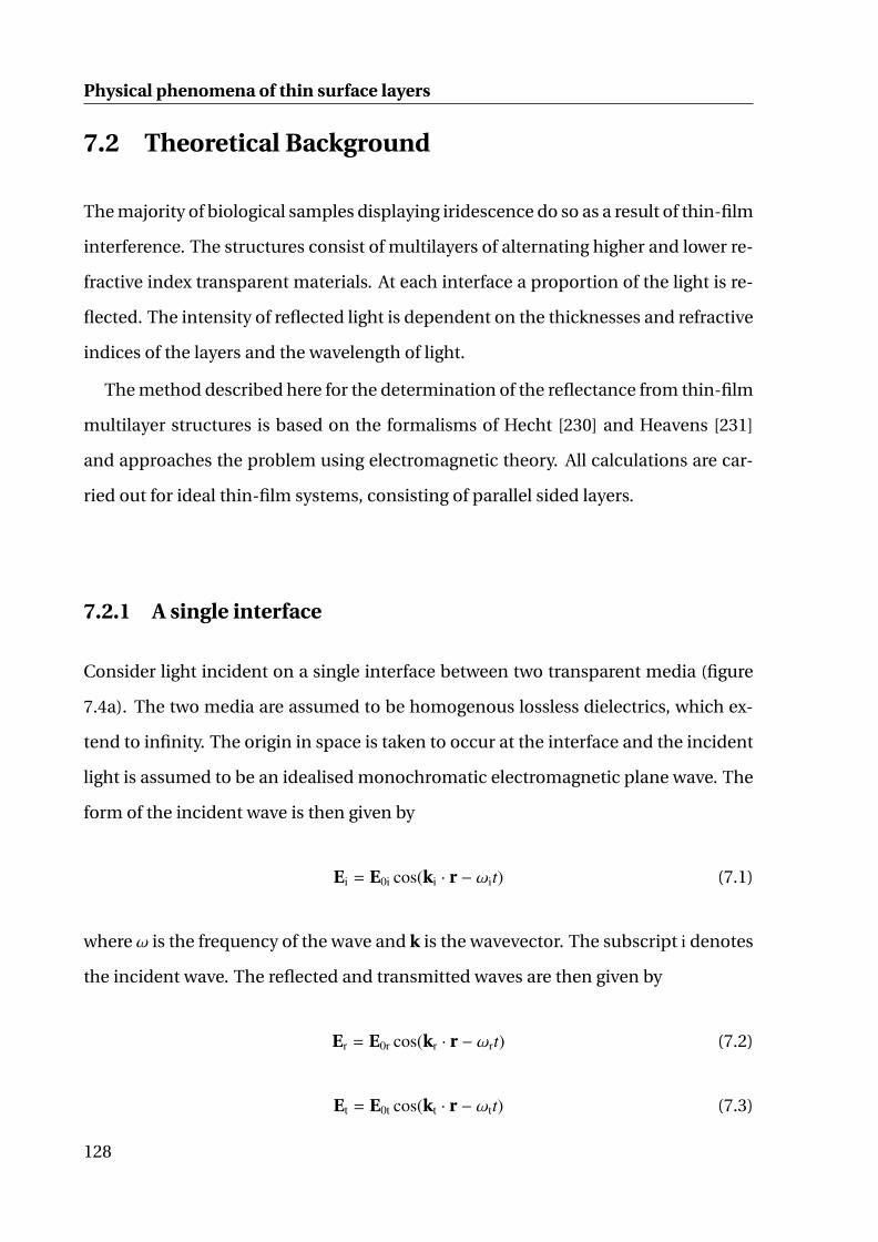
Physical phenomena of thin surface layers
7.2 Theoretical Background
The majority of biological samples displaying iridescence do so as a result of thin-film
interference. The structures consist of multilayers of alternating higher and lower re-
fractive index transparent materials. At each interface a proportion of the light is re-
flected. The intensity of reflected light is dependent on the thicknesses and refractive
indices of the layers and the wavelength of light.
The method described here for the determination of the reflectance from thin-film
multilayer structures is based on the formalisms of Hecht [230] and Heavens [231]
and approaches the problem using electromagnetic theory. All calculations are car-
ried out for ideal thin-film systems, consisting of parallel sided layers.
7.2.1 A single interface
Consider light incident on a single interface between two transparent media (figure
7.4a). The two media are assumed to be homogenous lossless dielectrics, which ex-
tend to infinity. The origin in space is taken to occur at the interface and the incident
light is assumed to be an idealised monochromatic electromagnetic plane wave. The
form of the incident wave is then given by
Ei = E0i cos(ki · r − ωit) (7.1)
where ω is the frequency of the wave and k is the wavevector. The subscript i denotes
the incident wave. The reflected and transmitted waves are then given by
Er = E0r cos(kr · r − ωrt) (7.2)
Et = E0t cos(kt · r − ωtt) (7.3)
128

Iridescence in tropical ferns
θi θr
θt
n0
n1
Interface
ki
kr
kt
Ei Er
Et
θi
θt
t01
t01t10r1S
t01r1S
t01r10r1S
r01
t 01r10r1S
2t01t10r10r1S
2d
air n0
1
substrate ns
a b
Figure 7.4: (a) Electromagnetic wave incident on an interface. (b) Successive reflected beamsacross a single film.
where the subscripts r, t denote the reflected and transmitted waves respectively.
Considering the laws of electromagnetic theory, the boundary condition that the tan-
gential component of E is continuous across the interface, must be satisfied. This
leads to the following
ωi = ωr = ωt (7.4)
θi = θr (7.5)
n0 sin θi = n1 sin θt (7.6)
Equation 7.5 and equation 7.6 are the Law of Reflection and Snell’s law respectively.
To find the amplitude of the reflected and transmitted waves, we consider sepa-
rately, the components of the electromagnetic field perpendicular and parallel to the
plane of incidence. Taking first the component of E perpendicular to the plane of
incidence, the boundary conditions require that E is continuous across the interface
such that
E0i + E0r = E0t (7.7)
while the normal component of εE must be the same on both sides of the interface.
129

Physical phenomena of thin surface layers
From this the perpendicular amplitude reflection and transmission coefficients can
be found, which are the ratios of E0r/E0i and E0t/E0i respectively.
rs =E0r
E0i=
n0 cos θi − n1 cos θt
n0 cos θi + n1 cos θt(7.8)
ts =E0t
E0i=
2n0 cos θi
n0 cos θi + n1 cos θt(7.9)
Considering now the component of E which lies in the plane of incidence, continuity
at the interface requires that
E0i cos θi − E0r cos θr = E0t cos θt (7.10)
remembering that θi = θr the parallel amplitude reflection and transmission coeffi-
cients can be found and are given by
rp =n0 cos θt − n1 cos θi
n0 cos θt + n1 cos θi(7.11)
tp =2n0 cos θi
n0 cos θt + n1 cos θi(7.12)
Together rp, rs, tp and ts are known as the Fresnel coefficients. The reflectance is de-
fined as the ratio of the reflected power to the incident power. When there is no ab-
sorption Rp = r2p, Rs = r2
s and the transmittance is given by2
T =
(n1 cos θt
n0 cos θi
)t2 (7.13)
7.2.2 A single thin film on a substrate
Consider now a thin dielectric film of thickness d deposited on a substrate, where the
refractive indices of the film and the substrate are n1 and ns respectively (figure 7.4b).
2R+T=1
130

Iridescence in tropical ferns
Both the substrate and air are considered to be non-absorbing layers. The incident
beam can be divided into its reflected and transmitted parts. The amplitudes of
successively reflected and transmitted beams can be written in terms of the Fresnel
equations given by equations 7.8-7.12. To find the reflectance characteristics we must
consider the reflected and transmitted waves at both the air/film interface and the
film/substrate interface. The Fresnel coefficient for light reflected from the air/film
interface is denoted by r01 and from the film/substrate interface by r1S, where light is
reflected toward the air layer. Similarly for light reflected from the film/air interface
the Fresnel coefficient is denoted by r10 and from the substrate/film interface by rS1,
where light is reflected in the direction of the substrate. The transmission coefficients
are similarly named.
From equations 7.8-7.12 we can see that r01 = −r10 and t01t10 = 1 − r201. The phase
change for a beam traversing the film is
δ1 =2πλ
n1d1 cos θt (7.14)
where λ is the wavelength of the light. The reflected amplitude is then found by con-
sidering the sum of the successive beams reflected at the air/film interface
r01S = r01 + t01t10r1S exp(−2iδ1) − t01t10r01r21S exp(−4iδ1) + ... =
r01 + r1S exp(−2iδ1)1 + r01r1S exp(−2iδ1)
(7.15)
7.2.3 Multilayer reflections
For a multilayer consisting of a stack of alternating dielectric media, medium 1 and
medium 2, with refractive indices n1, n2, the reflectance can be found by considering
each layer in turn (figure 7.5). Taking the bottom layer of the stack to be material 2
the reflection coefficient rbottom = r12S can be calculated using equation 7.15, where the
131

Physical phenomena of thin surface layers
air n0
material 1 n1 d1
material 2 n2 d2
substrate ns
n1
n2
ns
θi
θt d2
Step 1
θiθt
n2
n1
bottom
Step 2
a cb
Figure 7.5: (a)Multilayer stack of alternating layers of material 1 and material 2. (b) Step 1:Reflections at the bottom layer are considered to determine a virtual complex refractive indexof the bottom layer and the substrate. (c) Step 2: Reflections from the next layer up in thestack are considered taking into account the virtual refractive index of the bottom layer andthe substrate.
upper medium is medium 1 and the lower medium is the substrate.
rbottom = r12S =r12 + r2S exp(−2iδ2)
1 + r12r2S exp(−2iδ2)(7.16)
Moving one layer up in the stack medium 1 can now be thought of as being sand-
wiched between medium 2 and a semi-infinite layer for which rbottom is the Fresnel
coefficient. The reflection coefficient rnext is given by
rnext =r21 + rbottom exp(−2iδ1)
1 + r21rbottom exp(−2iδ1)(7.17)
This continues until the air interface is reached. The reflectance of the multilayer
stack is then R = r2stack.
7.3 Materials and Methods
Selaginella willdenowii plant material was obtained from The Royal Botanic Gardens
Kew, accession number 1994-1186-RONI 57. The plant was grown in a glass house
132

Iridescence in tropical ferns
Figure 7.6: (a)Photograph of Selaginella willdenowii plant grown at The Royal Botanical Gar-dens, Kew. (b) Blue juvenile leaf. (c) Mature green leaf.
under the following conditions: night temperature 18 C, day temperature 22 C, vent
temperature 25 C, humidity 70 − 80%. The plants were grown under normal sun-
light levels, with partial shading of the greenhouse for incident light with an intensity
greater than 100 W/m2 and full shading for incident light with an intensity greater than
200 W/m2. Plant material from the same plant was also kept at the Cambridge Uni-
versity Botanic Garden and grown under the same conditions, with partial shading
of the plant. A photograph of the plant grown at Kew can be seen in figure 7.6 along
with photographs of individual young and old leaves.
Spectroscopy
Spectroscopic reflection measurements of Selaginella willdenowii were carried out
using a fibre-optic based gonio-spectroscopic set-up, with independently adjustable
light incidence and collection angles. The set-up can be seen in figure 7.7. An Ocean
Optics DHL2000 light source with a combined deuterium halogen lamp provided a
collimated 2 mm wide beam for illumination of the samples with light in the spec-
tral range of 300 − 900 nm. Reflected or scattered light was detected with an Ocean
133

Physical phenomena of thin surface layers
θ θ I D
light sourcecollimating
lens
leaf sample
to spectroscope
scattered light2mm
iris
incident lightcollimated beam
a b
Figure 7.7: (a) Photograph of the gonio-spectroscope set up used. (b) Schematic representa-tion of (a).
Optics USB4000 spectroscope. The plant leaves were mounted on metal washers so
that the leaves were flat and free standing. Both specular reflection and scattering
measurements were carried out. For specular reflection measurements, the angle of
light incidence θI, measured from the sample surface normal, was varied from 16 to
60 in 2 steps. The detection angle was adjusted to θD = −θI in order to detect the
specularly reflected light. For scattering measurements, the angle of incidence was
fixed at 36 and the angle of detection was varied from 0 to 90. The reflection mea-
surements were normalised with respect to a Spectralon® diffuse reflectance stan-
dard of 99% reflectance. Absolute reflection measurements were carried out using a
Labsphere® integrating sphere. Measurements were carried out on a mature green
leaf and a semi-iridescent blue leaf.3
Microscopy
For ultrastructural studies small branches of the leaves were fixed in Karnovsky’s fixa-
tive (2% paraformaldehyde, 2.5% glutaraldehyde in 0.1 M phosphate buffer at pH 7.2)
overnight at 4 C. Sections 1 × 2 mm2 were then cut, rinsed in buffer and post-fixed
in a 1% osmium tetroxide (Agar) phosphate buffer solution for 2 hrs. They were then
rinsed in buffer and dehydrated in absolute ethanol solutions in steps from 30% EtOH
3Due to problems with growing the plants, a juvenile fully iridescent leaf was not available at thetime of the integrating sphere measurements.
134

Iridescence in tropical ferns
Tungsten lament
Electron Beam
Electro-magneticLens
Viewing Screen
Sample
a b
Figure 7.8: (a) Photograph of FEI Phillips Technai 20. (b) Schematic representation of (a).
to 100% EtOH. The material was embedded in optical grade LR Resin (Agar) and left
for one week at 4 C to allow the resin to infiltrate. The resin was changed daily. The
samples were cured under vacuum at 400 mbar for 20 hrs at 58 C. Thin sections were
cut using a Leica Ultracut UCT microtome and stained using a Leica EM stain with
uranyl acetate and lead citrate. Images were taken using a FEI Philips Tecnai 20 TEM
at 200 kV.
Surface structures were obtained by taking casts of the leaves in dental wax. The
cast was allowed to set. Once set the leaf was removed and the casts were then filled
with epoxy. After the epoxy had set, the dental wax cast was removed, leaving a posi-
tive replica of the plant leaf [232]. This was imaged using optical microscopy. Specu-
lar reflection and scattering measurements were also made on the epoxy casts.
Transmission electron microscopy
Transmission electron microscopy (TEM) was used for ultrastructural imaging of the
plant leaves. TEM allows for the imaging of thin sections of materials with a much
higher resolution than other microscopy techniques; the resolution of the TEM is lim-
ited to about 0.2 nm as compared to light microscopy which has a resolution limit of
0.2 µm [233].
135

Physical phenomena of thin surface layers
The sample is irradiated with a beam of electrons, focussed using electromagnetic
lenses. As the beam passes though the sample, the electrons interact with the sample.
The level of this interaction depends on the electron density of the material present;
the more dense a material, the more the electrons are scattered. A fluorescent screen
at the bottom of the microscope is used to image the transmitted electrons, forming a
‘shadow’ image, where the sample is imaged according to the density of the material.
More dense materials will appear darker, while less dense materials appear brighter.
A schematic representation of a TEM microscope can be seen in figure 7.8 along with
a photograph of the TEM used here.
Soft materials, such as plant leaves and polymers, often have a low scattering power
resulting in low contrast between different components. This contrast can be en-
hanced through the use of staining. Widely used stains for biological samples include
osmium tetroxide, uranyl acetate and lead citrate. Osmium tetroxide is used as a fix-
ative and while it does have some staining ability, the contrast, which comes from a
lack of unsaturated bonds in the specimen, is insufficient for epoxy resin sections,
such as those used here. Uranyl acetate and lead citrate are both general biological
stains with low specificity and are used to enhance the contrast of cells, tissues and
secretions. While each stain can be used on its own, double staining provides en-
hanced resolution of small features as more components of the sample are stained.
Results with lead citrate are also improved if osmium tetroxide has been used at some
point during the fixation procedure [234].
136

Iridescence in tropical ferns
7.4 Results
The spectroscopic measurements of the juvenile blue leaves and mature green leaves
can be seen in figure 7.9. Both leaves were taken from the same branch of the same
a b
c d
e f
300 400 500 600 700 8000.0
0.1
0.2
0.3
0.4
0.5
0.6
0.7 θ
θ
θ
θ
θ
θ
θ
Ref
lect
ance
λ300 400 500 600 700 800
0.0
0.1
0.2
0.3
0.4
0.5
0.6
0.7
Ref
lect
ance
λ[nm]
300 400 500 6000.0
0.1
0.2
Ref
lect
ance
λ[nm]300 400 500 600
0.0
0.1
0.2
Ref
lect
ance
λ[nm]
Figure 7.9: Specular reflection and scattering spectra of juvenile blue (left) and mature green(right) Selaginella willdenowii leaves. Intensity of specularly reflected light as a function oflight incidence angle for (a) juvenile blue leaves and (b) mature green leaves. (c) and (d) En-largement of the reflection peaks in the blue and green spectral range from (a) and (b), respec-tively. Scattered intensity as a function of detection angle for a fixed light incidence angle of36 for (e) juvenile blue leaves and (f) mature green leaves. The intensity is colour coded, withred (dark) corresponding to a lower intensity and yellow (bright) a higher intensity.
137

Physical phenomena of thin surface layers
300 400 500 600 700 8000.0
0.1
0.2
0.3
0.4
0.5
0.6
0.7
Ref
lect
ance
λ[nm]300 400 500 600 700 800
0.0
0.2
0.4
0.6
0.8
1.0
Ref
lect
ance
[abs
]
λ[nm]
a b
Figure 7.10: (a) Spectrally resolved specular reflection of juvenile blue (blue line) and maturegreen (green line) Selaginella willdenowii leaves at θI = −θD = 16. (b) Integrating spherereflection measurements of blue (blue line) and mature green (green line) leaves.
plant. The blue leaf was from the newest growth on the branch, while the green leaf
was from older growth. Leaves in between were seen to vary in colouration from blue
to green depending on age. For the juvenile blue leaves a peak in the reflectance
spectra is observed at around 430 nm in specular reflection, for an angle of incidence
θI = 16 (figure 7.10). This peak shifts to lower wavelengths when increasing θI from
16 to 50 (figure 7.9a, c) and is not present in the spectra measured for the mature
green leaves (figure 7.9b, d). In both sets of data a peak at 545 nm is observed. This
peak does not change position as θI is varied. The 545 nm peak has a 50% increased
reflectance in the green leaf compared to the blue leaf, but the overall reflectance of
both leaves is the same.
Figures 7.9e, f show the scattering measurements for the blue and green leaves
respectively, for θI = 36. The horizontal band at 545 nm stems from the green re-
flectance peak, seen for both leaves. This band is independent of the incidence and
detection angles. For higher |θD| a weak peak is observed in the scattering data at
around 450 nm in figure 7.9f, which is also present in the specular reflection measure-
ments (figure 7.9b). This suggests that the multilayer stack of the juvenile blue leaf is
still partially present in the green leaf. The different position of this peak in figure 7.9f
as compared to figure 7.9e suggests that the thicknesses and/or contrast between the
138

Iridescence in tropical ferns
a
b
c
d
e
f
c
Figure 7.11: TEM micrographs of the outer cell wall and the cuticle from the upper epidermisof (a) a juvenile blue leaf and (b) an older green leaf. Scale bar is 500 nm. Arrows indicate thelayers observed in the cuticle. Optical micrographs of surface morphology of plant cells for(c) a juvenile blue leaf and (d) a mature green leaf. Scale bar is 50 µm. (e) TEM micrographof juvenile blue leaf showing cell structure. Scale bar is 20 µm. (f) ESEM micrograph showingleaf structure of a juvenile blue leaf. Scale bar is 50 µm.
layers has changed as the leaf has aged. The gradual increase in broad-band intensity
for values from θD are intrinsic to our experimental configuration and independent
of the sample; the spot size on the sample, from which the light is detected, increases
with increasing |θD|.
Figure 7.10b shows the experimental spectra for the integrating sphere measure-
ments. The measurements were carried out on a mature green leaf and a semi-iridescent
blue leaf. The blue leaf, while being the youngest growth on the plant was not a juve-
nile leaf. The results give an indication of the absolute reflectance of the leaves and
show that the relative intensities of the leaves in the range 300 − 700 nm as measured
in specular reflection are comparable (figure 7.10a). The spectra are averaged over
three different measurements.
139

Physical phenomena of thin surface layers
300 400 500 600 700 8000.00
0.05
0.10
0.15
0.20
0.25R
efle
ctan
ce
λ [nm]
b
c
a
[h]
Figure 7.12: (a) Reflection of epoxy cast of a young blue leaf at θI = θD = 16. (b) Dentalwax cast of a juvenile blue leaf. (c) Epoxy cast of (b), this has been coated with platinum forcontrast.
Figure 7.11 shows cross-sectional TEM images of the blue and green Selaginella
willdenowii leaves. The images show the outer cell wall and the cuticle from the up-
per epidermis of the leaves. In figure 7.11a four distinct layers are observed in the
cuticle of the blue leaf, followed by a more disordered layer structure in the lower epi-
dermis. These alternating light and dark bands correspond to electron-transparent
and electron-opaque layers, respectively. This alternating layer structure is not vis-
ible in the cross-section of the green leaf (figure 7.11b). Instead, only a single dark
layer is discernible, followed by a more disordered lamellar structure. The cuticle of
the green leaf of ∼ 1.1 µm is much thicker as compared to the blue leaf ∼ 700 nm.
The surface structures of the blue and green leaves are shown in figures 7.11c, d.
There is very little difference between the two images, both show epidermal cells
arranged in disordered rows. The cells have a size on the order of 20 µm. Spectro-
scopic measurements of the epoxy casts show a constant reflectance for 300− 850 nm,
which corresponds to the reflection properties of the epoxy (figure 7.12). This con-
firms that the surface cell structure does not contribute to the blue colouration seen
in the young leaves.
140

Iridescence in tropical ferns
7.4.1 Modelling
The results show that the position of the peak wavelength seen at ∼ 430 nm decreases
as the angle of incidence increases. From this it is reasonable to assume that the
blue colour in the juvenile leaves comes from multilayer interference arising from the
four lamellae observed in the upper cuticle. Optical modelling of a 4-layer structure
was therefore used to account for the optical properties of the Selaginella willdenowii
leaves.
The thickness of each layer was measured from TEM cross-sections (figure 7.11a).
Layer one, the outermost layer, has a thickness of 66 ± 5 nm and layer two has a thick-
ness of 50 ± 5 nm (as measured from cross-sections taken of three different iridescent
leaves). The refractive index of cellulose is known to vary with the degree of hydra-
tion [235], with a more hydrated cellulose having a lower refractive index. It is there-
fore likely that the outer layer, L1, has a higher refractive index than the underlying
layer, L2, which is presumably less hydrated. The refractive index of the underlying
cell is approximately 1.36 as calculated by Charney et al. for the refractive index of
plant cell cytoplasm [236].
The model structure is shown schematically in figure 7.13a. The lamellae L1 and
L2, are approximated as homogeneous, transparent dielectric films with refractive in-
dices n1 and n2 and thicknesses d1 and d2. The reflectance of such a planar multilayer
structure can be calculated by propagating a plane wave through the stack, consid-
ering interfacial reflections and interference using Fresnel’s equations [237, 238] as
discussed in section 7.2.
The experimental spectra for θI = 16 and the corresponding model calculations,
are shown in figure 7.13b,d. While the model calculations allow us to confirm whether
the peak in the experimental reflectance data corresponds to that of the model, the
simple model does not predict the absolute intensity of the measured reflectance and
therefore cannot be compared using this method. While the blue colour clearly arises
141

Physical phenomena of thin surface layers
Experimental Data n1=1.45 n2=1.44 nout=1.36 Simplified leaf structure AR Coating 650nm n=1.24 d=130nm AR Coating 550nm n=1.24 d=110nm
300 400 500 600 7000.00
0.05
0.10
Ref
lect
ance
[Sim
ulat
ions
]
λ [nm]
0.00
0.05
0.10
0.15
0.20
0.25
nair = 1.0n1 = 1.45n2 = 1.44
nout = 1.36
d=66nmd=50nm
θ
θ
I
t
θD
a
b
0.86 0.88 0.90 0.92 0.94 0.96 0.98 1.00
400
420
440
460 Experimental Data Single layer d=232nm n=1.45 Four layers n1=1.45 n2=1.44 Four layers n1=1.45 n2=1.43 Four layers n1=1.45 n2=1.42
λ[nm
]
cos(θt)
ab c
cb a
L1L2
cd
Ree
ctan
ce [D
ata]
Figure 7.13: (a) Multilayer model. (b, d) Experimental data and simulated reflectance from anoptical multilayer with d1 = 66 nm and d2 = 50 nm, with different combinations of n1 and n2.(b) Simulations for a simplified leaf structure (dashed line) on top of a homogeneous opticalmedium. Simulated reflectance for the simplified leaf covered by an anti-reflective coatingoptimised for (red) 650 nm and (green) 550 nm, respectively. (d) Peak in the reflectance seenbetween 380 and 450 nm. Theoretical peak shift as calculated using (a) (blue line). Theoreticalpeak shift for other combinations of n1 and n2 (pink and green lines). Theoretical peak shiftfor a simplified structure with d = 232 nm (dashed line). Black points show experimental dataand are an average of three measurements. (c) Contributions from faces a, b and c for lightwith normal incidence and light with a higher incident angle.
from multilayer interference, the optical signal stemming from the overall structure
of the leaf is complex. Its optical signature is a superposition of Bragg interference
with intensities arising from scattering off irregularities at the surface and in the mul-
tilayer, backscattering of light from the cytoplasm and variations in the surface-normal
of the multilayer due to the cell shape and leaf curvature (see also below). The mea-
surements also do not take into account any polarisation effects of the multilayer; the
reflected intensity varies as a function of polarisation. All simulations shown here are
for unpolarised light.
142

Iridescence in tropical ferns
The model assumes that d1 = 66 nm, d2 = 50 nm, n1 = 1.45, n2 = 1.44 and nout = 1.36.
Figure 7.13d shows the wavelength λmax of the multilayer reflectance peak as a func-
tion of incidence angle for the juvenile blue leaves. The wavelength is averaged over
spectra from three different leaves. While the data extracted from the specular re-
flection experiments (points) are well described by the model calculation (blue line)
for small angles of incidence, the model and the data deviate for higher angles. The
model assumes planar, horizontally flat homogenous layers. The shape of the epider-
mal cells are however, dome-shaped (figure 7.11c). The cell morphology determines
the local optical geometry. For normal incidence, the flat top part of the cell locally
approximates the planar surface of the model in figure 7.13a. For larger incident an-
gles more light impinges on the cell edges, which now play an increasing role. The
local angle of light incidence at the illuminated cell edges is smaller than the global
incidence angle. The reflected intensity detected at θD = −θI results from superposi-
tion of the light that is specularly reflected from the top part of the cell and light that
scatters from the cell edges (figure 7.13c). The detected wavelength is consequently
red-shifted compared to the planar multilayer model, somewhat reducing the irides-
cent nature of the blue peak.
Other combinations of n1 and n2 were also simulated, to assess whether different
configurations would result in the same reflectivity behaviour. Figure 7.13d shows
that increasing the refractive index contrast between the two layers shifts the peak in
the reflectance to lower wavelengths than those found experimentally.
The small enhancement of the specular reflectance at around 450 nm for the green
leaf (figure 7.9b) seen at high angles is consistent with a double layer interference
filter with n1 = 1.45, d1 = 75 nm and n2 = 1.44, d2 = 25 nm. This corresponds to the two
partial lamellae seen in figure 7.13b. For small θI, this maximum broadens and shifts
to 500 nm, almost disappearing into the peak at 500 nm that results from scattering
pigments in the leaf.
143

Physical phenomena of thin surface layers
7.5 Discussion
Our detailed reflectance measurements show that the blue colouration seen in juve-
nile Selaginella willdenowii leaves is iridescent and stems from the four-layer inter-
ference filter in the cuticle on the upper surface of the leaves. The blue iridescence
disappears as the leaf ages. The TEM images and reflection data suggest that the loss
in the blue colouration comes from a degradation or increasing disorder of the mul-
tilayer structure, starting with the lower layers. For the older green leaves, only weak
double layer interference is still present.
Modelling of the data suggests that the refractive index contrast between the two
layers is on the order of 0.01. This difference is very small compared to other opti-
cal multilayers found for example in beetles and butterflies. Here however, the layer
structure consists of only one material and the refractive index variation arises from a
difference in hydration. This strongly limits the achievable refractive index contrast.
The comparison of model calculations with experimental spectra confirms that the
observed blue iridescence can arise from such a weak refractive index contrast.
Figure 7.9e shows a blue reflection band stretching across a wide range of detec-
tion angles. The ideal planar Bragg multilayer assumed in the model calculations
would result instead in a localised specular signal at θD = θI (i.e. at sin θD ≈ −0.6)
with little intensity at other angles. The wide blue intensity band of figure 7.9e stems
from the disorder in the surface-normal of the multilayer. This disorder arises from
the cell shape and from the curvature of the leaves. As a result, parts of the leaf lo-
cally fulfil Bragg’s condition for any observation angle causing the angle-invariance
of the observed colour. A similar optical response is seen for other natural multilayer
structures. For example, the blue iridescence of Morpho rhetenor has a similar angle-
invariance arising from the curvature of the multilayers on its wing-scales [239, 240].
The simple model used to describe multilayer interference therefore only approxi-
mates the optical response of the complex surface structures found in nature.
144

Iridescence in tropical ferns
Modelling of the data shows that the multilayer structure preferentially reflects
light in the blue part of the spectrum, a photosynthetically important spectral region,
which is deficient in the light present in the natural habitat of these shade-dwelling
plants. In this low-light environment the light is enriched in the R:FR part of the spec-
trum. Lee et al. have suggested that the blue-reflecting multilayer more effectively
couples the long optical wavelength into the leaf, thereby enhancing photosynthesis.
Our more detailed data allows the testing of this hypothesis.
A comparison of figures 7.9a and b shows that the reflectance in the 600 − 700 nm
spectral range is strongly angle dependent. For the more important small angles of
incidence, the average log wavelength reflectance is comparable. This is best seen in
figure 7.10 where reflectance of the green leaf dips below the that of the blue leaf for
∼ 660 nm, the maximum for red-absorption of chlorophyll.
Due to the complex optical signature of leaves, it is instructive to address the ques-
tion of enhanced red-adsorption in terms of model calculations. The dashed line in
figure 7.13b is the prediction for a simplified leaf structure consisting only of an op-
tically dense top cuticle layer and an optically less dense lower phase. The predicted
optical response of this simplified leaf structure in the 600-700 nm spectral range is
very similar to the model 4-layer structure of the blue leaf. While this comparison
illustrates the unsuitability of the multilayer to couple red light into the leaves, it is
perhaps instructive to compare the measured spectra to optical coatings that are op-
timised for this effect.
Antireflective coatings consisting of a bilayer of low and high refractive index ma-
terials are well known. The optimisation condition for such a bilayer is noutn21 = n2
2,
with λ/4 thicknesses for each layer [242]. Superimposing the simplified leaf (dashed
line in figure 7.13b) with a 110 – 130 nm thick layer of refractive index n = 1.24 signif-
icantly reduces the reflected light not only for the optimised wavelengths of 550 nm
(dash-dotted line) and 650 nm (dotted line), respectively, but over most of the visible
spectrum. The possibility of optical coatings consisting of porous or nanostructured
145

Physical phenomena of thin surface layers
(b)
(c)
(a)
(b)
Figure 2. Corneal nipple arrac-aureum (a) and the lycae
(a)
(b)
(a)
(b)
Figure 2. Corneal nipple arrac-aureum (a) and the lycae
(a)
(b)
(b)
(c)
(d)
(e)
of a surface layer in which the refractive index variesgradually from unity to that of the bulk material ( WilsoHutley 1982 ). The insight that nipple arrays can stronglyreduce surface reflectance has been widely technicallyapplied, e.g. in window panes, cell phone displayscamera lenses (rev. Palasantzas et al. 2005 ; for fuinformation and explanatory figures, see, for example
(b)
Figure 2. Corneal nipple arrays in the nymphalid Polygoniac-aureum (a) and the lycaenid Pseudozizeeria mahshowing di erences in nipple height and shape. Bar, 500
a
b
c
d
e
Figure 7.14: (a) Complete eye of the peacock nymphalid butterfly Inachis io. (b) Nipple arrayof one facet lens of (a). Corneal nipple array in (c) the nymphalid Bicyclus anynana, (d) the ly-caenid Pseudozizeeria maha and (e) in Inachis io. Scale bars (a) 500 µm, (b) 5 µm, (c,d) 500 nmand (e) 2 µm. Pictures taken from [241].
cuticle, becomes evident when considering the coatings found on the eyes of moths
and on butterfly wings [241], where a wide variety of optically active nanostructures
are observed (figure 7.14).
Figure 7.10 shows that the juvenile blue leaves have a lower reflectance between
500−600 nm as compared to the mature green leaves and a similar reflectance between
600 − 700 nm. A similar behaviour is seen for Danaea nodosa, where the iridescence
is seen in the juvenile leaves and disappears in the adult leaves due to the loss of the
multilayer structures responsible for the iridescence [222]. Graham et al. also studied
the difference in the optical properties of twelve rainforest sun and thirteen rainforest
146

Iridescence in tropical ferns
extreme shade plants [243], including iridescent species. Their results show that the
absorption spectra of sun and extreme shade plants are identical apart from a small
increase for the shade plants at 550 nm. Our data and model calculations show that
the role of blue iridescence in Selaginella willdenowii is not to couple in more red
light, refuting the hypothesis by Lee et al.
7.6 Possible adaptive advantages of iridescence
A taxonomically diverse range of photosynthetic organisms, from diatoms [244] to
algae [245–247] through to angiosperms [222], produce a vivid iridescence over the
surface of their photosynthetic apparatus. An equally diverse range of methods are
used to produce this iridescence. This strongly suggests that the production of irides-
cence has evolved multiple times and has some unknown adaptive advantage for life
in deep shade.
Our results show that it is unlikely that a multilayer structure acts to increase light
capture in photosynthetically important wavelength ranges under low light condi-
tions in this case, since no enhancement of absorption by the blue leaves is seen in
the red part of the spectrum. While an interesting hypothesis, this idea is counter in-
tuitive for a number of reasons. Firstly, it makes no sense that the plant would want
to sacrifice the absorption of any incident blue light in favour of red light. Blue light
is important for both photosynthesis and plant development.
Secondly, the multilayer filter does not act as an effective anti-reflective coating.
As shown in figure 7.13b, a simple strategy to implement a broad-band antireflective
coating consists of the deposition of a low refractive index (n = 1.24) λ/4 layer on top
of a generic leaf surface. Compared to optical multilayers, a porous or structured low
refractive index surface layer is optically more robust and presumably less resource
intensive for the plant. The evolutionary feasibility of this is well documented in in-
sects [241]. Stavenga et al. show that the papillae seen on the eyes of butterflies,
147

Physical phenomena of thin surface layers
act to produce a graded refractive index surface layer, which acts as an antireflective
surface.
Increased capture of photosynthetically important wavelengths is not the only adap-
tive advantage that leaf iridescence may offer. Others include a visual defence against
herbivores, a photoprotective mechanism to protect shade-adapted plants against
sun-flecks and other potentially damaging sudden high light levels and a polarisa-
tion filter enhancing orientation of photosynthetic apparatus within the cell.
A visual defence against herbivores
Whitney et al. have recently shown that insects can see iridescence independently of
any other cue [202]. Iridescence can act to increase detectability due to the changing
colour of the object when perceived from different angles, delivering more stimu-
lus to the photoreceptors of the eye. However, this may come with a cost; the very
changeability of iridescence that increases detectability could corrupt object iden-
tity, making it harder for insects to form a search image [248]. In certain situations
this potential corruption of identity could be a significant advantage. The constantly
changing colours produced by iridescence would alternatively blend or contrast with
any background, producing an effect similar to conventional disruptive colouration,
like that of the zebra [249, 250]. The iridescence produced on the leaves of plants
could act to confuse moving insects and herbivores by camouflaging the shape and
edge of the leaf and making it difficult to form a target search image.
Alternatively the iridescence may serve to deter herbivores by causing the leaves
to look sufficiently different to all other food sources that iridescent leaves are not
recognised as food, or avoided. Evidence for these hypotheses has been found in the
iridescent alga Mazzaella flaccida, where non-iridescent thalli of this seaweed were
seen to suffer more from herbivory than their iridescent counterparts [247].
148

Iridescence in tropical ferns
A photoprotective mechanism
All of the plants that produce blue leaf iridescence grow in extremely sheltered low-
light environments and as such are thought to be strongly shade-adapted. Such plants
would be extremely vulnerable to photodamage if even transiently exposed to sun
flecks (where small patches of light break through the canopy), due to the increased
sensitivity of their photosynthetic apparatus. The constructive interference produced
by the blue leaf iridescence in the wavelengths of 400−485 nm may therefore function
to protect against photoinhibition (the inhibition of photosynthesis due to exces-
sive irradiance) and damage via reduced light absorption at those wavelengths [251].
Light attenuation mechanisms have been suggested for other shade dwelling plants,
which have red leaves due to the presence of anthocyanins. These pigments are seen
to function in light attenuation by intercepting quanta which would otherwise be ab-
sorbed by the chlorophyll, protecting the leaves from photoinhibition when exposed
to sun flecks [214, 252].
A polarisation filter
If optimised for this purpose, optical multilayers can enhance the polarisation of light
that occurs upon reflection and transmission at each surface. Ferns in particular have
been shown to respond to light polarised in a particular plane, a response known as
polarotropism [253]. Two features of plants appear to be key for the polarotropic
response, the ordering of the cellulose fibrils within the cell wall and plant photore-
ceptors with a dichroic function.
There are two potential functions that iridescence could be fulfilling if its role is to
act as a polarisation filter. Firstly, polarisation of light might enhance orientation of
photosynthetic apparatus within the plant cell and thus increases photosynthetic ef-
ficiency [254,255]. Secondly, by determining the plane of light polarisation additional
information about a rare resource might be obtained.
Theories of how polarised light may be used as an additional environmental cue
149

Physical phenomena of thin surface layers
are found mainly in the insect vision literature. The spider Dracones cupreus has a
pair of specialised secondary eyes that, like the iridescent leaves of Selaginella willde-
nowii, strongly reflect blue light. These eyes act as polarising filters, with one eye per-
mitting the passage of horizontally polarised light, the other permitting the passage
of vertically polarised light. The spider can use the ratio of light in each eye to deter-
mine the polarisation angle of light around it in the environment, which in turn can
be used for navigation [256].
In the forest environment in which shade-adapted iridescent plants occur, direct
sunlight is obscured. While the light that has been transmitted through other leaves
is unpolarised, any light that is reflected from the vertical sides of trees is generally
perpendicularly polarised and light reflected from leaves is predominately parallel
polarised [257, 258]. The polarisation of light reflected from leaves under these con-
ditions could potentially provide more detail about the surrounding environment,
allowing modulation of development of physiological processes to maximise fitness.
In particular, changes to the polarisation environment resulting from the fall of trees
might provide opportunities for light capture or threats to sensitive photosynthetic
machinery, both of which might result in plant acclimation. It would therefore inter-
esting to include polarisation measurements in future quantitative optical studies of
Selaginella willdenowii.
7.7 Conclusions
In summary, it has been shown that the blue colouration seen in the leaves of Se-
laginella willdenowii is indeed iridescent. For an angle of incidence of 16 a peak in
the reflectance spectra is observed at 430 nm. As the angle of incidence is increased,
this peak shifts to lower wavelengths.
Transmission electron microscopy studies reveal a layered lamellar structure in
the upper epidermis of the leaves. Modelling of the thin film multilayer structures
150

Iridescence in tropical ferns
confirms that they are responsible for the iridescence observed in the leaves. As the
leaves age the blue colouration is seen to disappear, with older leaves of the same
plant appearing green. Comparison of the juvenile blue and mature green leaves
indicates that the loss of blue iridescence corresponds to a loss and disorder of the
multilayer structures.
The results reported here do not support the idea that iridescence in Selaginella
willdenowii acts to enhance light capture of photosynthetically important wavelengths.
The reflectance of light in the range 600 − 700 nm is the same for both iridescent and
non-iridescent leaves. However, due to the occurrence of blue colouration in a wide
variety of shade dwelling plants it is likely that this iridescence has some other adap-
tive benefit.
151


CHAPTER
EIGHT
CONCLUSIONS
This thesis covers a number of different thin film phenomena, from the intrinsic be-
haviour and stability of thin films, to their potential use in hard-drive disk technolo-
gies, to the stunning optical effects that films can be used to produce. This chapter
summarises the main conclusions of the work, discuss their implications and possi-
ble directions for future research.
Thin film polymer blends
In chapter 3 the stability of thin film polystyrene (PS)/ poly(vinylmethylether) (PVME)
blends was investigated. These polymers are miscible at room temperature and phase
separate upon heating. The behaviour of varying blend compositions was studied at
temperatures where the PS and PVME are miscible. The PVME was seen to enrich
the polymer/air interface, forming a layer with a width comparable to the correla-
tion length of the PVME. Further heating close to the demixing temperature resulted
in the formation of capillary instabilities at the polymer surface. These exhibited a
spinodal-like pattern with a characteristic wavelength dependent on the blend com-
position. The formation of these instabilities was observed for all blend compositions
investigated.
153

Physical phenomena of thin surface layers
Dr. Nigel Clarke at the University of Durham had previously shown, using a ther-
modynamic model, that when thin binary mixture films are subject to coupled height
and composition fluctuations, the film is more unstable than if either the height or
concentration fluctuations are considered in isolation. In collaboration with Clarke,
his model was adapted for this system, taking into account the composition depen-
dent Hamaker constant and the experimental parameters. The model showed good
agreement with the experimental data, suggesting that the instabilities observed in
the blend resulted from coupled height and composition fluctuations within the PVME
wetting layer.
The formation of instabilities was only observed when the blends were heated
close to the demixing temperature. PVME wetting layers were also observed to form
at the polymer/air interface for blends kept at room temperature for extended peri-
ods of time. These blends were stable; no instabilities were seen. It would be inter-
esting to find the temperature at which the blends become unstable and whether the
annealing temperature, influences the wavelength of the instabilities that form.
Non-equilibrium behaviour of thin films
In chapter 4 thin films were destabilised using an electric field, in order to probe the
effects of sample preparation on the rheology and stresses within the film. Films were
spun from five different solvents: toluene, trans-decalin, chloroform, tetrahydrofu-
ran and methylethylketone. The casting solvent had a strong effect on the onset time
and the wavelength of the instabilities that formed.
The characteristic time of destabilisation is directly proportional to the film viscos-
ity. The experimental onset times were much smaller than those predicted from lin-
ear stability analysis using bulk viscosity of the polymer and varied with casting sol-
vent quality. The discrepancy is explained in terms of non-equilibrium effects caused
by the spin coating process; the fast evaporation of the solvent from the films during
spin coating creates a lower entanglement density in the film compared to that of an
154

Conclusions
equilibrium melt. This results in an increased mobility of the chains. The difference
between the films spun from the various solvents can be explained by the changes in
chain conformations in the initial solutions and the amount of solvent remaining in
the film at vitrification.
The characteristic wavelength of the instabilities in as-cast films was observed to
be higher than the theoretical value, indicating a weak stabilising pressure in the
films. These could arise from frozen-in normal stresses in the as-cast films. In ad-
dition the wavelength was dependent on the casting solvent, with the greatest wave-
length being observed for films spun from toluene and the smallest for films spun
from trans-decalin. It is suggested that spin-coating results in an asymmetric defor-
mation of the chains due to evaporation of the remaining solvent in the film after vit-
rification. This deformation is possibly dependent on the conformation of the chains
prior to vitrification and on the molecular weight of the polymer.
Both the frozen-in normal stresses and viscosity deviations were removed upon
annealing the films above the glass transition temperature. The time scale on which
the frozen-in stresses were removed was much less than the annealing time required
to restore bulk viscosity. This suggests that local rearrangements of the chains are suf-
ficient to remove the anisotropy responsible for the residual stress. Recovery of bulk
viscosity however, requires complete equilibration of the chains and much longer an-
nealing times.
The results indicate that the boiling point of the solvent, the film formation time,
the solubility of PS in the solvent and the amount of solvent remaining in the film
on vitrification are all significant. No single property could be used to consistently
describe the trends observed in the data. Instead the behaviour observed must result
from a combination of all of these parameters.
The behaviour observed in these experiments can being explained in terms of the
entanglements of the polymer chains. On these length scales, the chains can be con-
sidered as being far from equilibrium in the as-cast films. In polymer films the glass
155

Physical phenomena of thin surface layers
transition temperature has been observed to deviate from the bulk value, even when
relatively thick films are investigated. The reason for this deviation is not well under-
stood.
The glass transition temperature is dependent on effects happening on the seg-
mental length scale of the polymer chain. This work shows that the polymer chain
is far from equilibrium at the entanglement length scale and raises questions about
what is happening on the segmental length scale. Are the chains also far from equi-
librium on the segmental length scale and is this responsible for the deviations in
the glass transition temperature observed? A possible extension of this project would
be to prepare polymer films as far from equilibrium as possible. By using a Langmuir-
Blodgett1 technique for example, films could be built up chain-by-chain with no inter-
chain entanglements. Studying both the glass transition and the rheology of such a
film may provide some answers as to how the two length scales are connected and
why a decrease in the glass transition temperature is observed.
Magnitude of residual stress in thin films
In chapter 5 the feasibility of using focused ion beam milling to study the overall
magnitude of the stresses in as-cast films was investigated. Cantilevers were cut into
PS films spun-cast onto low stress silicon nitride membranes. On completion of the
milling the cantilevers were observed to bend upwards. By modelling the cantilever
as a plate, the stresses in the polymer film were calculated from the deflection of the
cantilever. For as spun films the stress was measured to be 211 MPa, with a reduction
being observed for films aged at room temperature.
While this chapter shows the feasibility of this method for measuring the magni-
tude of stored stresses in polymer films, the results seem to contradict those of chap-
ter 4. For the cantilever to bend, the film must be in a state of tensile stress. Such a
stress should drive instability formation, resulting in a smaller wavelength of insta-
1Langmuir-Blodgett films are deposited monolayer by monolayer and are normally formed fromamphiphilic molecules with a hydrophilic head and a hydrophobic tail e.g. fatty acids.
156

Conclusions
bility forming with a faster onset time. This is opposite to the behaviour observed in
chapter 4.
The combination of these results and those in chapter 4 therefore suggest that the
stress distribution within the film is more complex than a simple uniform in-plane
stress or frozen-in normal stress. The nature of the stresses in as-cast polymer films
is thus not yet fully understood.
Magnetic thin films
In chapter 6 the magnetic properties of ceramic films pyrolysed from palladium doped
polyferrocenylethylmethylsilane (PFEMS) were investigated. The palladium was added
in nanoparticle form and through directly mixing palladium acetylacetonate with
the polymer prior to film deposition. The polymer precursors were all seen to ex-
hibit paramagnetic behaviour. Increasing magnetic susceptibility was observed with
palladium content. Pyrolysis of the polymer precursors resulted in the formation of
ferromagnetic ceramics. The magnetic behaviour was seen to depend on the tem-
perature and atmosphere used for pyrolysis. Pyrolysis of the palladium containing
precursors under argon at 1000 C, resulted in the formation of ceramics containing
FePd alloys. These ceramics had an enhanced coercivity, remanent magnetisation
and saturation magnetisation.
The formation of FePd alloys is highly desirable due to their application in data
storage technologies. Metal alloy nanoparticles and films are normally prepared us-
ing methods such as sputter deposition under ultra high vacuum, electrodeposition
and chemical vapour deposition. All of these methods require specialist equipment,
can be costly and are time consuming. Here the incorporation of palladium into
the iron-containing PFEMS, allows for FePd containing ceramics to be formed. This
would enable iron-palladium containing ceramics to be produced quickly and cheaply
in a one step process.
To be relevant for data storage technologies, structured films are required with
157

Physical phenomena of thin surface layers
feature sizes on the order of 50 nm. Iron-containing polymers have previously been
structured on the nanoscale using an imprint method. This pattern is retained on
pyrolysis. Future work will focus on using similar methods to pattern the palladium
doped PFEMS. This would allow a regular array of ceramic pillars to be formed with
the required properties, providing an alternative to current data storage technologies.
Iridescent thin films
Finally, in chapter 7 the bright blue colouration observed on the leaf of the tropical
fern Selaginella willdenowii was studied. This fern grows in the understorey of the
rainforest where the light intensity is less than 1% of that at the canopy. The blue
colouration is shown to be iridescent in nature, with a peak in the reflectance spectra
for the juvenile blue leaves being observed at around 430 nm for an angle of incidence
of 16. This peak shifts to lower wavelengths as the angle of incidence is increased
and is not observed in more mature green leaves.
Transmission electron microscopy studies confirm the presence of a layered lamel-
lar thin film structure on the upper cuticle of the iridescent leaves. These thin film
multilayers were modelled using literature values for the refractive indices of the plant
cell cytoplasm and cuticular wax, showing that they are responsible for the irides-
cence observed. Blue and green leaves from the same plant were compared. The loss
of the blue iridescence corresponds to a loss of the multilayer structures.
It had previously been postulated that the iridescence in these plants might act to
enhance light capture of photosynthetically important wavelengths. The results in
chapter 7 do not support this hypothesis. The reflectance of light in the range of 600−
700 nm is the same for both the iridescent and non-iridescent leaves. Blue iridescence
is not confined to Selaginella willdenowii, but is observed in a wide variety of shade
dwelling photosynthetic organisms. As a result it is likely that the iridescence has
some other adaptive benefit. While some possibilities are discussed in chapter 7,
further investigations are required before any conclusions, on the role of iridescence,
158

Conclusions
in these plants can be made. Insight into the role of the iridescence could be achieved
through identification of the genes that control production of the iridescence. So far
identification of these genes, in both plants and animals, has eluded biologists. If the
genes could be found and implanted into non-iridescent species, direct comparison
of iridescent and non-iridescent plants could be carried out. It would also allow for
some pretty cool plants to be grown!
159


BIBLIOGRAPHY
[1] M Geoghegan and G Krausch. Wetting at polymer surfaces and interfaces. Prog.
Polym. Sci., 28(2):261–302, 2003.
[2] F Bruder and R Brenn. Spinodal decomposition in thin films of a polymer
blend. Phys. Rev. Lett., 69(4):624–627, 1992.
[3] H Wang and J Composto. Thin film polymer blends undergoing phase separa-
tion and wetting: Identification of early, intermediate and later stages. J. Chem.
Phys., 113(22):10386–10397, 2000.
[4] QS Bhatia, DP Pan, and JT Koberstein. Preferential surface adsorption in mis-
cible blends of polystyrene and poly(vinyl methyl ether). Macromolecules,
21:2166–2175, 1988.
[5] E Schäffer, T Thurn-Albrecht, TP Russell, and U Steiner. Electrically induced
structure formation and pattern transfer. Nature, 403:874–877, 2000.
[6] ZQ Lin, T Lerle, TP Russell, E Schaffer, and U Steiner. Structure formation at the
liquid/liquid bilayer in electric fields. Macromolecules, 35:3971–3976, 2002.
[7] D Barbero and U Steiner. Nonequilibrium polymer rheology in spin-cast films.
Phys. Rev. Lett., 102:248303, 2009.
[8] MJ MacLachlan, M Ginzburg, N Coombs, TW Coyle, NP Raju, JE Greeden,
GA Ozin, and Manners I. Shaped ceramics with tunable magnetic properties
from metal-containing polymers. Science, 287:1460–1463, 2000.
[9] P Vukusic and R Sambles. Photonic structures in biology. Nature, 424:852–855,
2003.
[10] PJ Flory. Thermodynamics of high polymer solutions. J. Chem. Phys., 10:51–61,
1942.
161

Physical phenomena of thin surface layers
[11] ML Huggins. Some properties of solutions of long-chain compounds. J. Chem.
Phys., 146:1942, 151-158.
[12] XF Gong, KS Shing, and WV Chang. Effect of composition dependent flory in-
teraction parameter χ on polymer adsorption theory. Polym. Bull., 22:71–78,
1989.
[13] J Eckelt, R Sugaya, and BA Wolf. Pullulan and dextran: Uncommon compo-
sition dependent flory-huggins interaction parameters of their aqueous solu-
tions. Biomacromolecules, 9:1691–1697, 2008.
[14] S Qian, SJ Mumby, and BE Eichinger. Phase diagrams of binary polymer solu-
tions and blends. Macromolecules, 24:1655–1661, 1991.
[15] M Rubenstein and RH Colby. Polymer Physics. Oxford University Press, Oxford,
2006.
[16] E Schäffer, S Harkema, M Roerdink, R Blossey, and U Steiner. Morphological
instability of a confined polymer film in a thermal gradient. Macromolecules,
36:1645–1655, 2003.
[17] M Nedelcu, MD Morariu, D Harkema, NE Voicu, and U Steiner. Pattern forma-
tion by temperature-gradient driven film instabilities in lateral geometries. Soft
Matter, 1:62–65, 2005.
[18] A Oron, SH Davis, and SG Bankoff. Long-scale evolution of thin liquid films.
Rev. Mod. Phys., 69(3):931–980, 2002.
[19] R Seeman, S Herminghaus, C Neto, S Schlagowski, D Podzimek, R Konrad,
H Mantz, and K Jacobs. Dynamics and structure formation in thin polymer
melt films. J. Phys.-Condes. Matter, 17(9):S267–S290, 2005.
[20] MB Williams and SH Davis. Nonlinear theory of film rupture. J. Colloid Interface
Sci., 90(1):220–228, 1982.
[21] G Reiter. Dewetting of thin polymer-films. Phys. Rev. Lett., 68(1):75–78, 1992.
[22] G Reiter. Unstable thin polymer films: Rupture and dewetting processes. Lang-
muir, 9(9):1344–1351, 1993.
[23] A Pototsky, Bestehorn. M, D Merkt, and U Thiele. Evolution of interface pat-
terns of three-dimensional two-layer liquid films. Europhys. Lett., 74(4):665–
671, 2006.
162

Bibliography
[24] A Sharma and J Mittal. Instability of thin liquid films by density varia-
tions: A new mechanism that mimics spinodal dewetting. Phys. Rev. Lett.,
89(18):186101, 2002.
[25] E Schäffer. Instabilities of thin polymer films: structure formation and pattern
transfer. PhD thesis, Universitat Konstanz, 2001.
[26] F London. Zur theorie und systematik der molekularkrafte. Z Phys., 63:245–279,
1930.
[27] R Seeman, S Herminghaus, and K Jacobs. Dewetting patterns and molecular
forces: A reconciliation. Phys. Rev. Lett., 86:5534–5537, 2001.
[28] J Israelachvili. Intermolecular and Surface Forces. Academic Press„ London,
1991.
[29] R Yerushalami-Rozen, T Kerle, and J Klein. Alternative dewetting pathways of
thin liquid films. Science, 285:1254–1255, 1999.
[30] S Madruga and U Thiele. Decomposition driven interface evolution for layers
of binary mixtures. ii. influence of connective transport on linear stability. Phys.
Fluids, 21:062104, 2009.
[31] VI Kovalchuk, H Kamusewitz, D Vollhardt, and NM Kovalchuk. Auto-oscillation
of surface tension. Phys. Rev. E, 60(2):2029–2036, 1999.
[32] U Thiele, S Madruga, and L Frastia. Decomposition driven interface evolution
for layers of binary mixtures. i. model derivation and stratified base states. Phys.
Fluids, 19:122106, 2007.
[33] N Clarke. Instabilities in thin-film binary mixtures. Eur. Phys. J. E, 14(3):207–
210, 2004.
[34] N Clarke. Toward a model for pattern formation in ultra-thin binary mixtures.
Macromolecules, 38(16):6775–6778, 2005.
[35] MD Morariu, NE Voicu, E Schaffer, Z Lin, TP Russell, and U Steiner. Heirarchical
structure formation and pattern replication induced by an electric field. Nat.
Mater., 2:48–52, 2003.
[36] P Goldberg-Oppenheimer and U Steiner. Rapid electrohydrodynamic lithogra-
phy using low-viscosity polymers. Small, 6(11):1248–1254, 2010.
163

Physical phenomena of thin surface layers
[37] JW Swan. Stress and other effects produced in resin and in a viscid compound
of resin and oil by electrification. P. Roy. Soc. London, 62:38–46, 1897.
[38] A Onuki. Interface instability induced by an electric field in fluids. Physica A,
217:38–52, 1995.
[39] S Herminghaus. Dynamical instability of thin liquid films between conducting
media. Phys. Rev. Lett., 83(12):2359–2361, 1999.
[40] LF Pease and WB Russel. Limitations on length scales for electrostatically in-
duced submicrometer pillars and holes. Langmuir, 20:795–804, 2004.
[41] X Li, L Wu, P Deshpande, Z Yu, W Wu, H Ge, and SY Chou. 100nm period grat-
ings produced by lithographically induced self-construction. Nanotechnology,
14:786–790, 2003.
[42] P Deshpande, LF Pease III, L Chen, SY Chou, and WB Russel. Cylindrically
symmetric electrohydrodynamic patterning. Phys. Rev. E, 70:041601, 2004.
[43] NE Voicu, S Harkema, and U Steiner. Electric-field-induced pattern morpholo-
gies in thin liquid films. Adv. Funct. Mater., 16:926–934, 2006.
[44] U Steiner. Force measurements using capillary instabilities. J. Polym. Sci. Pol.
Phys., 43(23):3395–3405, 2005.
[45] U Steiner. Nanoscale assembly. Chemical techniques. Springer, 2005.
[46] U Steiner and J Klein. Growth of wetting layers from liquid mixtures. Phys. Rev.
Lett., 77(12):2536–2529, 1996.
[47] U Steiner, J Klein, E Eiser, A Budkowski, and LJ Fetter. Complete wetting from
polymer mixtures. Science, 258(5085):1126–1129, 1992.
[48] JMG Cowie, BG Devlin, and IJ McEwan. Surface enrichment in ps/pvme blends:
2. the effect of specific interaction in the bulk mixture. Polymer, 34(19):4130–
4135, 1993.
[49] PG deGennes. Wetting: statics and dynamics. Rev. Mod. Phys., 57(3):827–863,
1985.
[50] PG deGennes. Scaling concepts in polymer physics. Cornell University Press,
Ithaca, 1979.
164

Bibliography
[51] J Genzer and RJ Composto. Surface segregation and amplification in miscible
blends near criticality. Europhys. Lett., 38(3):171–176, 1997.
[52] MD Morariu, E Schäffer, and U Steiner. Capillary instabilities by fluctuation
induced forces. Eur. Phys. J. E, 12(3):375–381, 2003.
[53] J You, Y Liao, X Li, Z Su, and L An. Temperature dependence of surface compo-
sition and morphology in polymer blend film. Polymer, 49:4456–4461, 2008.
[54] RAL Jones, LJ Norton, EJ Kramer, FS Bates, and P Wiltzius. Surface-directed
spinodal decomposition. Phys. Rev. Lett., 66(10):1326–1329, 1991.
[55] HP Fischer, P Maass, and W Dieterich. Diverging time and length scales of
spinodal decomposition modes in thin films. Europhys. Lett., 42(1):49–54, 1998.
[56] HP Fischer, P Maass, and W Dieterich. Novel surface modes in spinodal de-
composition. Phys. Rev. Lett., 79(5):893–896, 1997.
[57] Y Nishi and TK Kwei. Cloud point curves for poly(vinyl methyl ether) and
monodisperse polystyrene mixtures. Polymer, 16:285–290, 1975.
[58] T Shiomi. Thermodynamics of polymer blends of poly(vinyl methyl ether) and
polystyrene. Macromolecules, 23:229–233, 1990.
[59] K El-Mabrouk. Assessment of morphology in transient and steady state regimes
resulting from phase separation in polystyrene/poly(vinyl methyl ether). Rheol.
Acta., 45:877–889, 2006.
[60] A Ajji, L Choplin, and RE Prudhomme. Rheology of polystyrene poly(vinyl
methyl ether) blends near the phase transition. J. Poly. Sci. B: Poly. Phys.,
29(13):1573–1578, 1991.
[61] MB Djordjevic and PS Porter. C-13 nmr characterisation of intermolecular in-
teractions for polymers. Poly. Eng. Sci., 22:1109–1116, 1982.
[62] PA Mirau and JL White. Solid state nmr studies of intermolecular interactions
in solid polymer blends. Magn. Reson. Chem., 32:S23–S29, 1994.
[63] B Reidl and RE Prudhomme. Temperature dependence of the interaction pa-
rameter between n-heptane, carbon-tetrachloride and benzene and poly(vinyl
methyl ether) between 120c and 180c. J. Poly. Sci. B, 28:2411–2420, 1990.
165

Physical phenomena of thin surface layers
[64] M Bank, J Leffingwell, and C Thies. The influence of solvent upon the compati-
bility of polystyrene and poly(vinyl methyl ether). Macromolecules, 4(1):43–46,
1971.
[65] CC Han, BJ Bauer, JC Clark, Y Muroga, Y Matsushuta, M Okada, Q Tran-cong,
and T Chang. Temperature, composition and molecular weight dependence
of the binary interaction parameter of polystyrene/poly(vinyl methyl ether)
blends. Polymer, 29:2002–2014, 1988.
[66] El-Mabrouk. K and M Bousmina. Effect of molecular weight and shear on phase
diagram of ps/pvme blend. Rheol. Acta., 45:959–969, 2006.
[67] K El-Mabrouk, M Belaiche, and M Bousmia. Phase separation in ps/pvme thin
and thick films. J. Colloid Interf. Sci, 306(2):354–367, 2007.
[68] RM Briber and BJ Bauer. Effect of cross-links on the phase separation behaviour
of a miscible polymer blend. Macromolecules, 21:3296–3303, 1988.
[69] C Forrey, JT Koberstein, and DH Pan. Surface segregation in miscible blends
of polystyrene and poly(vinyl methyl ether): Comparison of theory and experi-
ment. Interface Sci., 11:211–223, 2003.
[70] DH Pan and WM Prest. Surface of polymer blends: x-ray photoelectron-
spectroscopy studies of polystyrene/ poly(vinyl methyl ether) blends. J. Appl.
Phys., 58(8):2861–2870, 1985.
[71] D Wang and H Ishida. Surface microscale semi-heterogeneous structures in
compatible polystyrene and poly(vinyl methyl ether) blend thin films investi-
gated by lateral-force microscopy. Macromol. Chem. Physic., 208(19-20):2222–
2228, 2007.
[72] H Wang and RJ Composto. Wetting and phase separation in polymer blend
films: Identification of four thickness regimes with district morphological path-
ways. Interface Sci., 11(11):237–248, 2003.
[73] T Nishi, TT Wang, and TK Kwei. Thermally induced phase separation behaviour
of compatible polymer mixtures. Macromolecules, 8(2):227–234, 1975.
[74] H Ogawa, T Kanaya, and G Matsuba. Composition fluctuations before dewet-
ting in polystyrene/ poly(vinyl methyl ether) blend thin films. Polymer,
49:2553–2559, 2008.
166

Bibliography
[75] T Wagler, PL Rinaldi, CD Han, and H Chun. Phase behaviour and segmental
mobility in binary blends of polystyrene and poly(vinyl methyl ether). Macro-
molecules, 33:1778–1789, 2000.
[76] A Asano, K Takegoshi, and K Hikichi. C-13 cp/mass nmr-study on the mis-
cibility and phase-separation of a polystyrene poly(vinyl methyl ether) blend.
Macromolecules, 35(26):5630–5636, 1994.
[77] K Takegoshi and K Hikichi. Effects of blending on local chain dynamics and
glass transition: polystyrene/ poly(vinyl methyl ether) blends as studied by
high-resolution solid-state 13c nuclear magnetic resonance spectroscopy. J.
Chem. Phys., 94(4):3200–3206, 1991.
[78] TK Kwei, T Nichi, and RF Roberts. A study of compatible polymer mixtures.
Macromolecules, 7(5):667–674, 1974.
[79] K Schmidt-Rohr, J Clauss, and HW Spiess. Correlation of structure, mo-
bility and morphological information in heterogeneous polymer materials
by two-dimensional wideline-separation nmr spectroscopy. Macromolecules,
25(12):3273–3277, 1992.
[80] R Brown, editor. Handbook of polymer testing. Marcel Dekker Inc., New York,
1999.
[81] P Duckworth, H Richardson, C Carelli, and JL Keddie. Infrared ellipsometry of
interdiffusion in thin films of miscible polymers. Surf. Inter. Anal., 36:33–41,
2004.
[82] K Hinrichs, M Gensch, N Nikonenko, J Pionteck, and KJ Eichhorn. Spectro-
scopic ellipsometry for characterization of thin films of polymer blends. Macro-
mol. Symp., 230:26–32, 2005.
[83] BB Sauer and DJ Walsh. Use of neutron reflection and spectroscopic ellipsom-
etry for the study of the interface between miscible polymer blends. Macro-
molecules, 24(22):5948–5955, 1991.
[84] TP Russell. The characterization of polymer interfaces. Annu. Rev. Mater. Sci.,
21:249–268, 1991.
[85] JE Mark, editor. Polymer Data Handbook. Oxford University Press, online edi-
tion, 1999.
167

Physical phenomena of thin surface layers
[86] J Brandrup, EH Immergrut, and EA Grulke, editors. Polymer Handbook, volume
1 and 2 of New Jersey. Wiley-Interscience, fourth edition, 1999.
[87] DE Aspnes. Local-field effects and effective-medium theory: A microscopic
perspective. Am. J. Phys., 50:8, 1982.
[88] RP Feynman, RB Leighton, and M Sands. The Feynman Lectures on Physics,
volume 2. Addison-Wesley Publishing Company, Reading, MA, 1965.
[89] DAG Bruggeman. Calculation of various physics constants in heterogeneous
substances 1. dielectric constants and conductivity of mixed bodies from
isotropic substances. Ann. Physik, 416(8):665–679, 1935.
[90] R Gelles and CW Frank. Phase separation in polystyrene/poly(vinyl methyl
ether) blends as studied by excimer fluorescence. Macromolecules, 15:1486–
1491, 1982.
[91] RAL Jones and RW Richards. Polymers at Surfaces and Interfaces. Cambridge
University Press, Cambridge, 1999.
[92] M Shibayama, H Yang, RS Stein, and CC Han. Study of the miscibility and criti-
cal phenomena of deuterated polystyrene and hydrogenated poly(vinyl methyl
ether) by small angle neutron scattering. Macromolecules, 18:2179–2187, 1985.
[93] RAL Jones, EJ Kramer, MH Rafailovich, J Sokolov, and SA Schwarz. Surface en-
richment in an isotropic polymer blend. Phys. Rev. Lett., 62(3):280–283, 1989.
[94] T Gal. Functional differentiation under conservation constraints. J. Phys. A:
Math, Gen., 35:5899–5905, 2005.
[95] T Gal. Differentiation of functionals with variables coupled by conserva-
tion constraints: Analysis though a fluid-dynamical model. J. Math. Phys.,
48:053520, 2007.
[96] SF Edwards. Proc. Phys. Soc., 88(2):365–280, 1966.
[97] M Souche and N Clarke. Phase equilibria in polymer blend thin films: A hamil-
tonian approach. J. Chem. Phys., 131:244903, 2009.
[98] JL Keddie, RAL Jones, and RA Cory. Size-dependent depression of the glass
transition temperature in polymer films. Europhys. Lett., 27(1):59–64, 1994.
168

Bibliography
[99] T Miyazaki, K Nishida, and T Kanaya. Contraction and reexpansion of polymer
thin films. Phys. Rev. E, 69:022801, 2004.
[100] M Mukherjee, M Bhattacharya, MK Sanyal, Th Geue, J Grenzer, and U Pietsch.
Reversible negative thermal expansion of polymer films. Phys. Rev. E,
66:061801, 2002.
[101] J-L Masson and PF Green. Viscosity of entangled polystyrene thin film melts:
film thickness dependence. Phys. Rev. E, 65:031806, 2002.
[102] RL Jones, SK Kumar, DL Ho, RM Briber, and TP Russell. Chain conformation in
ultrathin polymer films. Nature, 400:146–149, 1999.
[103] H Kim, A Rühm, LB Lurio, JK Basu, J Lal, SGJ Mochrie, and SK Sinha. Syn-
chrotron radiation studies of the dynamics of polymer films. J. Phys. Condens.
Matter, 16:S3491–S3497, 2004.
[104] H Kim, A Rühm, LB Lurio, JK Basu, J Lal, D Lumma, SGJ Mochrie, and SK Sinha.
Surface dynamics of polymer films. Phys. Rev. Lett., 90(6):068302, 2003.
[105] G Reiter, S Al Akhrass, M Hamieh, P Damman, S Gabriele, T Vilmin, and
E Raphaël. Dewetting as an investigative tool for studying properties of thin
polymer films. Eur. Phys. J. Special Topics, 166:165–172, 2009.
[106] G Reiter, M Hamieh, P Damman, S Sclavons, S Gabriele, T Vilmin, and
E Raphaël. Residual stresses in thin polymer films cause rupture and dominate
early stages of dewetting. Nat. Mater., 4:754–758, 2005.
[107] P Damman, S Gabriele, S Coppee, S Desprez, D Villier, T Vilmin, E Raphaël,
M Hamieh, S Al Akhrass, and G Reiter. Relaxation of residual stress and reen-
tanglement of polymers in spin-coated films. Phys. Rev. Lett., 99:036101, 2007.
[108] T Vilmin and E Raphaël. Dewetting of thin polymer films. Eur. Phys. J. E, 21:161–
174, 2006.
[109] Z Yang, C-H Lam, E DiMasi, N Bouet, J Jordon-Sweet, and OKC Tsui. Method to
measure the viscosity of nanometer liquid films from surface fluctuations. App.
Phys. Lett., 94:251906, 2009.
[110] D Barbero. Study of the rheology of thin liquid films - novel flexible molds for
nanoimprinting. PhD thesis, University of Cambridge, 2009.
169

Physical phenomena of thin surface layers
[111] OKC Tsui, YJ Wang, FK Lee, C-H Lam, and Z Yang. Equilibrium pathway of
spin-coated polymer films. Macromolecules, 41:1465–1468, 2008.
[112] JH Park and E Kim. Effect of electric-field assisted thermal annealing of poly(4-
vinylphenol) film on its dielectric constant. App. Phys. Lett., 92(10):103311,
2008.
[113] TG Fox and PJ Flory. Second order transition temperatures and related proper-
ties of polystyrene. 1. influence of molecular weight. J. Appl. Phys., 21:581–591,
1950.
[114] EM Meyer, H Hug, and R Bennewitz. Scanning probe microscopy: The lab on a
tip. Springer-Verlag., Berlin, 2003.
[115] JC Moreira and NR Demarquette. Influence of temperature, molecular weight
and molecular weight dispersity on the surface tension of ps, pp and pe. 1. ex-
perimental. J. Appl. Polym. Sci., 82(8):1907–1920, 2001.
[116] T Vilmin and E Raphaël. Dynamic instability of thin viscoelastic films under
lateral stress. Phys. Rev. Lett., 97:036105, 2006.
[117] A Bach, K Almdal, HK Rasmussen, and O Hassanger. Elongational viscosity of
narrow molar mass distribution polystyrene. Macromolecules, 36:5174–5179,
2003.
[118] S-T Sun, I Nishio, G Swislow, and T Tanaka. The coil-globule transition: Radius
of gyration of polystyrene in cyclohexane. J. Chem. Phys., 73(12):5971–5875,
1980.
[119] M Daoud and G Jannink. Temperature-concentration diagram of polymer so-
lutions. J. Phys-Paris, 37:973–979, 1976.
[120] SH Maron and CA Daniels. Thermodynamics of polystyrene solutions 1. in-
teraction parameters and polymer order. J. Macr. Science Part B, 2(4):743–767,
1968.
[121] SR Quake. Topological effects of knots in polymers. Phys. Rev. Lett.,
73(24):3317–3320, 1994.
[122] Q Zhou and RG Larson. Direct molecular dynamics simulation of branch point
motion in asymmetric star polymer melts. Macromolecules, 40:3443–3449,
2007.
170

Bibliography
[123] Y Zhang, Q Ren, and Y Zhao. Modelling analysis of surface stress on a rectan-
gular cantilever beam. J. Phys. D: Appl. Phys., 37:2140–2145, 2004.
[124] W Fang and JA Wickert. Determining mean and gradient residual stresses in
thin films using micromachined cantilevers. J. Micromech. Microeng., 6:301–
309, 1996.
[125] GG Stoney. The tension of metallic films deposited by electrolysis. Proc. R. Soc.
Lond. A, 82:172–175, 1909.
[126] M Ree, S Swanson, and W Volksen. Effect of precursor history on residual stress
and relaxation behaviour of high temperature polyimides. Polymer, 34(7):1423–
1430, 1993.
[127] SG Croll. Internal stress in a solvent-cast thermoplastic coating. J. Coating.
Technol., 50(638):33–38, 1978.
[128] SG Croll. The origin of residual internal stress in solvent-cast thermoplastic
coatings. J. Appl. Polym. Sci., 23:847–858, 1979.
[129] JW Judy. Microelectromechanical systems (mems):fabrication, design and ap-
plications. Smart. Mater. Struct., 10:1115–1134, 2001.
[130] AM Korsunsky, M Sebastiani, and E Bemporad. Focused ion beam ring drilling
for residual stress evaluation. Mater. Lett., 63:1961–1963, 2009.
[131] N Sabate, D Vogel, A Gollhardt, J Keller, C Cane, I Gracia, JR Morante, and
B Michel. Measurement of residual stress by slot milling with focused ion-beam
equipment. J. Micromech. Microeng., 16:254–259, 2006.
[132] S Reyntjens and R Puers. A review of focused ion beam applications in mi-
crosystems technology. J. Micromech. Microeng., 11:287–300, 2001.
[133] EM Corcoran. Determining stresses in organic coatings using plate beam de-
flection. J. Paint Technol., 41:635–640, 1969.
[134] TS Chow, CA Liu, and RC Penwell. Strains induced upon drying thin films
solvent-cast on flexible substrates. J. Polym. Sci. Pol. Phys., 14:1311–1316, 1976.
[135] Z Rongjing. Mechanical characterisation of thin films with application to ferro-
electrics. PhD thesis, California institute of technology, 2006.
171

Physical phenomena of thin surface layers
[136] BA Walmsley, Y Liu, ZH Zhi, MB Bush, JM Dell, and L Farone. Poisson’s ra-
tio of low-temperature pecvd silicon nitride thin films. J. Microelectromech. S.,
16:622–627, 3 2007.
[137] JY Chung, Q Chastek, MJ Fasolka, HW Ro, and CM Stafford. Quantifying resid-
ual stress in nanoscale thin polymer films via surface wrinkling. ACS Nano,
3:844–852, 4 2009.
[138] RA Shalliker, PE Kavanagh, IM Russell, and Hawthorne. The measurement of
molecular weight distribution of some polydisperse polystyrene by reversed
phase and size exclusion chromatography. Chromatographia, 33:427–433,
1992.
[139] RD Mathad, HGH Kumar, B Sannakki, S Ganesh, KSS Sarma, and MV Badiger.
High energy electron irradiation effects on polystyrene films. Radiat. Eff. Defect.
S., 164:656–664, 10 2009.
[140] RDA Hudson. Ferrocene polymers: current architectures, syntheses and utility.
J. Organometallic Chemistry, 637:47–69, 2001.
[141] BW Rockett and G Marr. Ferrocene: Annual survey covering the year 1977. J.
Organometallic Chemistry, 167:51–134, 1979.
[142] KJ Wynne and RW Rice. Ceramics via polymer pyrolysis. Ann. Rev. Mater. Sci.,
14:297–334, 1984.
[143] AS Abd-El-Aziz and EK Todd. Organoiron polymers. Coord. Chem. Rev., 246:3–
52, 2003.
[144] TJ Kealy and PL Paulson. A new type of organo-iron compound. Nature,
168:1039–1040, 1951.
[145] I Manners. Putting metals into polymers. Science, 294:1665–1667, 2001.
[146] PD Pomogalio. Catalysis by polymer immobilized metal complexes. Gordon and
Breach Science Publishers, Amsterdam, 1998.
[147] RP Kingsborough and TM Swager. Transition metals in polymeric π-conjugated
organic frameworks. Prog. Inorg. Chem., 48:123, 1999.
[148] JA Massey, MA Winnik, and I Manners. Fabrications of oriented nanoscopic ce-
ramic lines from cylindrical micelles of an organometallic polyferrocene block
copolymer. J. Am. Chem. Soc., 123(13):3147–3148, 2001.
172

Bibliography
[149] V Bellas and M Rehahn. Polyferrocenylsilane-based polymer systems. Angew.
Chem. Int. Ed., 46:5082–5104, 2007.
[150] DE Herbert, UFJ Mayer, and I Manners. Strained metallocenophanes and re-
lated organometallic rings containing pi-hydrocarbon ligands and transition-
metal centers. Angew. Chem. Int. Ed., 46(27):5060–5081, 2007.
[151] B-Z Tang, R Petersen, DA Foucher, A Lough, N Coombs, R Sodhi, and I Man-
ners. Novel ceramic and organometallic depolymerisation products from
poly(ferrocenylsilanes) via pyrolysis. J. Chem. Soc. Cem. Commun., pages 523–
525, 1993.
[152] P Petersen, DA Foucher, B-Z Tang, A Lough, NP Raju, JE Greedan, and I Man-
ners. Pyrolysis of poly(ferrocenylsilanes): Synthesis and chacterization of fer-
romagnetic transition metal-containing ceramics and molecular depolymeri-
sation products. Chem. Mater., 7:2045–2053, 1995.
[153] M Ginzburg, MJ MachLachlan, SM Yang, N Coombs, TW Coyle, NP Raju,
JE Greeden, RH Herber, GA Ozin, and I Manners. Genesis of nanostructured,
magnetically tunable ceramics, from the pyrolysis of cross-linked polyferro-
cenylsilane networks and formation of shaped macroscopic objects and mi-
cron scale patterns by micromolding inside silicon wafers. J. Am. Chem. Soc.,
124(11):2625–2639, 2002.
[154] K Kulbaba, A Cheng, A Bartole, S Greenberg, R Resendes, N Coombs, S Safa-
Sefat, JE Greenden, HDH Stover, GA Ozin, and Manners I. Polyferrocenylsi-
lane microspheres: Synthesis, mechanism of formation, size change tunability,
electrostatic self-assembly and pyrolysis to spherical magnetic ceramic parti-
cles. J. Am. Chem. Soc., 124:12522–12534, 2002.
[155] Q Sun, JWY Lam, K Xu, H Xu, JAK Cha, PCL Wong, G Wen, X Zhang, X Jing,
F Wang, and BZ Tang. Nanocluster-containing mesoporous magnetoceram-
ics from hyperbranched organometallic polymer precursors. Chem. Mater,
12:2617–2624, 2000.
[156] D Chung. Carbon, 39:379, 2001.
[157] K Kulbaba and I Manners. Polyferrocenylsilanes: Metal-containing polymers
for materials science, self-assembly and nanostructure applications. Macro.
Rap. Comm., 22(10):711–724, 2001.
173

Physical phenomena of thin surface layers
[158] C-L Liu, Kand Ho, S Aouba, Y-Q Zhao, Z-H Lu, Si Petroc, N Coombs, P Dube,
H E. Ruda, W-Y Wong, and I Manners. Synthesis and lithographic patterning of
FePt nanoparticles using a bimetallic metallopolyyne precursor. Angew. Chem.-
Int. Edit., 47(7):1255–1259, 2008.
[159] K Liu, SB Clendenning, L Friebe, WY Chan, X Zhu, MR Freeman, GC Yang,
CM Yip, D Grozea, ZH Lu, and I Manners. Pyrolysis of highly metatalized poly-
mers: ceramic thin films containing magnetic cofe alloy nanoparticles from a
polyferrocenylsilane with pendant cobalt clusters. Chem. Mater., 18:2591–2601,
2006.
[160] L Friebe, K Liu, B Obermeier, S Petrov, P Dube, and I Manners. Pyrolysis of poly-
carbosilanes with pendant nickel clusters: synthesis and characterisation of
magnetic ceramics containing nickel and nickel silicide nanoparticles. Chem.
Mater, 19(10):2630–2640, 2007.
[161] GJ Nieuwenhuys. Magnetic behavior of cobalt, iron and manganese dissolved
in palladium. Adv. Phys., 24(4):515–591, 1975.
[162] H Naganuma, K Sato, and Y Hirotsu. Particle size dependence of atomic order-
ing and magnetic properties of l10-fepd nanoparticles. J. Magn. Magn. Mater.,
310:2356–2358, 2007.
[163] ME Gruner and A Dannenberg. Structure and magnetism of near-
stoichiometric fepd nanoparticles. J. Magn. Magn. Mater., 321(7):861–864,
2009.
[164] D Weller and MF Doerner. Extremely high-density longitudinal magnetic
recording media. Annu. Rev. Mater. Sci., 30:611–644, 2000.
[165] DA Rider, KA Cavicchi, KN Power-Billard, TP Russell, and I Manners. Di-
block copolymers with amorphous atactic polyferrocenylsilane blocks:
Synthesis, characterization, and self-assembly of polystyrene-block-
poly(ferrocenylethylmethylsilane) in the bulk state. Macromolecules, 38:6931–
6938, 2005.
[166] S Horiuchi, MI Sarwar, and Y Nakao. Nanoscale assembly of metal clusters in
block copolymer films with vapor of a metal-acetylacetonato complex using a
dry process. Adv. Mater., 12(20):1507–1511, 2000.
[167] RL Fagaly. Superconducting quantum interference device instruments and ap-
plications. Rev. Sci. Instrum., 77:101101, 2006.
174

Bibliography
[168] D Cohen. Magnetoencephalography: Detection of the brain’s electrical activity
with a superconducting magnetometer. Science, 175:664–666, 1972.
[169] J Clarke. Geophysical applications of squids. IEEE trans. magn., 19(3):288–294,
1972.
[170] H Weinstock, editor. SQUID sensors: Fundamentals, Fabrication and Applica-
tions, volume 329 of Series E: Applied Sciences. Kluwer Academic Publishers,
1995.
[171] C Hammond. The basics of crystallography and diffraction. Oxford Science
Publications, New York, 1997.
[172] S Lee, H Younan, Z Siping, and M Zhiqiang. Studies on electron penetration
versus beam acceleration voltage in dispersive x-ray molecules. pages 610–613,
Kuala Lumpar, Malaysia, 2006. ICSE2006 Proc.
[173] DA Rider, K Liu, J-C Eloi, L Vanderark, L Tang, J-Y Wang, D Grozea, Z-H
Lu, TP Russell, and I Manners. Nanostructured magnetic thin films from
organometallic block copolymers: Pyrolysis of self-assembled polystyrene-
block-poly(ferrocenylethylmethylsilane). ACS Nano, 2(2):263–270, 2008.
[174] V Cominos and A Gavriilidis. Sublimation and deposition behaviour of palla-
dium (ii) acetylacetonate. Eur. Phys. J. Appl. Phys, 15:25–33, 2001.
[175] A Guinier. X-Ray Diffraction in crystals, imperfect crystals and amorphous bod-
ies. General Publishing Company, Toronto, Canada, 1994.
[176] KJ Bryden and YY Jackie. Electrodeposition synthesis and hydrogen absorption
properties of nanostructures palladium-iron alloys. Nanastruc. Mater., 9:485–
488, 1997.
[177] W Li and P Haldar. Supportless pdfe nanorods as highly active electrocata-
lyst for proton exchange membrane fuel cell. Electrochem. Commun., 11:1195–
1198, 2009.
[178] WH Meiklejohn and CP Bean. New magnetic anisotropy. Phys. Rev., 102:1413,
1956.
[179] I Dzyaloshinsky. A thermodynamic theory of weak ferromagnetism of antifer-
romagnets. J. Phys. Chem. Solids, 4:241, 1958.
175

Physical phenomena of thin surface layers
[180] O Crisan, K von Haeften, AM Ellis, and C Binns. Structure and magnetic prop-
erties of fe/fe oxide clusters. J. Nanopart. Res., 10:193–199, 2008.
[181] E Zhang, Y Tang, K Peng, C Guo, and Y Zhang. Synthesis and magnetic prop-
erties of γ fe2o3/sio2 coreshell nanoparticles under hydrothermal conditions.
Solid State Commun., 148:496–500, 2008.
[182] LE Wenger, GM Tsoi, PP Vaishnava, U Senaratne, EC Buc, R Naik, and VM Naik.
Magnetic properties of γ fe2o3 nanoparticles precipitated in alginate hydro-
gels. IEEE T. Magn., 44(11):2760–2763, 2008.
[183] MP Fernandez, DS Schmool, AS Silva, M Sevilla, AB Fuertes, P Gorria, and
JA Blanco. Control of crystalline phases in magnetic fe nanoparticles inserted
inside a matrix of porous carbon. J. Magn. Magn. Mater., 322:1300–1303, 2010.
[184] S Veintemillas-Verdaguer, MP Morales, and CJ Serna. Continuous production
of gamma-fe2o3 ultrafine powders by laser pyrolysis. Mater. Lett., 35:227–231,
1998.
[185] RM Bozorth. Ferromagnetism. IEEE Press, USA, 1993.
[186] M Zayat, F Monte, MP Morales, G Rosa, H Guerro, CJ Serna, and D Levy. Highly
transparent γ fe2o3/vycor-glass magnetic nanocomposites exhibiting faraday
rotation. Adv. Mater., 15(21):1809–1812, 2003.
[187] AR Deshpande, H Xu, and JMK Wiezorek. Effects of grain size on coercivity of
combined-reaction-processed fepd intermetallics. Acta Mater., 52:2903–2911,
2004.
[188] S Wagner and A Pundt. Mechanical stress impact on thin pd1−xfex film thermo-
dynamic properties. Appl. Phys. Lett., 92:051914, 2008.
[189] SC Tjong and H Chen. Nanocrystalline materials and coatings. Mat. Sci. Eng.
R., 45:1–88, 2004.
[190] JKW Wang, TS Jung, J-B Chang, RA Mickiewicz, A Alexander-Katz, CA Ross, and
KK Berggren. Complex self-assembled patterns using sparse commensurate
templates with locally varying motifs. Nat. Nanotechnol., 5:256–260, 2010.
[191] VP Chuang, J Gwyther, RA Mickiewicz, I Manners, and CA Ross. Templated self-
assembly of square symmetry arrays from an abc tri-block terpolymer. Nano.
Lett., 9(12):4363–4369, 2009.
176

Bibliography
[192] K Liu, S Fournier-Bidoz, GA Ozin, and I Manners. Highly ordered magnetic ce-
ramics nanorod arrays from a polyferrocenylsilane by nanoimprint lithography
with anodic alluminium templates. Chem. Mater., 21:1781–1783, 2009.
[193] P Vukusic. Structural colour in lepidoptera. Curr. Bio., 16:R621–R623, 2006.
[194] M Srinivasarao. Nano-optics in the biological world: Beetles, butterflies, birds
and moths. Chem. Rev., 99(7):1935–1962, 1999.
[195] JP Vigneron, M Rassart, Z Vértesy, K Kertész, M Sarrazin, LP Biró, D Ertz, and
V Lousse. Optical structure and function of the white filamentary hair covering
the edelweiss bracts. Phys. Rev. E, 71:011906, 2005.
[196] AE Seago, P Brady, JP Vigneron, TD Schultz, and M Meadows. Gold bugs and
beyond: a review of iridescence and structural colour mechanisms in beetles
(coleoptera). J. R. Soc. Interface, 6:S165–S184, 2009.
[197] M Doucet and M Meadows. Iridescence: A functional perspective. J. R. Soc.
Interface, 6:S115–S132, 2009.
[198] A Loyau. Iridescent structurally based colouration of eyespots correlates with
mating success in the peacock. Behav. Ecol., 18:1123–1131, 2007.
[199] LP Biró, Z Bálint, K Kertész, Z Vértesy, GL Márk, ZE Hováth, J Balázs, D Méhn,
I Kiricsi, V Lousse, and JP Vigneron. Role of photonic-crystal-type structures in
the thermal regulation of a lycaenid butterfly sister species pair. Phys. Rev. E,
67:021907, 2003.
[200] RH Douglas and NJ Marshal. A review of vertebrate and invertebrate ocular
filters. In Adaptive mechanisms in the ecology of vision. Springer Publishing
Company, 1999.
[201] LP Biró, Z Bálint, Z Vértesy, K Kertész, GL Márk, V Lousse, and JP Vigneron.
Living photonic crystals: Nanostructure of the scales of Cyanophrys remus but-
terfly. Nanopages, 1(2):195–208, 2006.
[202] HM Whitney, M Kolle, P Andrew, L Chittka, U Steiner, and BJ Glover. Floral
iridescence, produced by diffractive optics, acts as a cue for animal pollinators.
Science, 323(5910):130–133, 2009.
[203] S Yoshioka and S Kinoshita. Effect of macroscopic structure in iridescent color
of the peacock feathers. Forma., 17:169–181, 2002.
177

Physical phenomena of thin surface layers
[204] P Vukusic. Taken from website http://newton.ex.ac.uk/research/emag/butterflies/
iridescence_in_nature.html, March 2010.
[205] H Whitney, M Kolle, R Alvarez-Fernandez, U Steiner, and B Glover. Contribu-
tions of iridescence to floral patterning. Comm. Int. Bio., 2(3):230–232, 2009.
[206] BJ Glover and HM Whitney. Structural colour and iridescence in plants: the
poorly studied relations of pigment colour. Ann. Bot., 105:505–511, 2010.
[207] DW Lee, GT Taylor, and AK Irvine. Structural fruit colouration in delarbrea
michieana (araliaceae). Int. J. Plant Sci., 161:297–300, 2000.
[208] TW Mulroy. Spectral properties of heavily glaucous and non-glaucous leaves of
a succulent rosette-plant. Oecologica, 38:349–357, 1979.
[209] JB Clark and GR Lister. Photosynthetic action spectra of trees. ii. the relation-
ship of cuticle structure to the visible and ultraviolet spectral properties of nee-
dles from four coniferous species. Plant Physiol., 55:407–413, 1975.
[210] QON Kay, HS Daoud, and CH Stirton. Pigment distribution, light-reflection and
cell structure in petals. Bot. J. Linn. Soc., 83:57–83, 1981.
[211] TC Volgelmann. Plant tissue optics. Ann. Rev. Plant Phys., 44:231–251, 1993.
[212] PW Richards. The tropical rainforest. Cambridge University Press, Cambridge,
2nd edition, 1996.
[213] DW Lee, JB Lowry, and BC Stone. Abaxial anthocyanin layers in leaves of trop-
ical rainforest plants - enhancer of light capture in deep shade. Biotropica,
11(1):70–77, 1979.
[214] NM Hughes, TC Vogelmann, and WK Smith. Optical effects of abaxial antho-
cyanin on absorption of red wavelengths by understorey species: revisiting the
back scatter hypothesis. J. Exp. Bot., 59:3435–3442, 2008.
[215] DW Lee. On the economy of plant form and function, chapter 4. Cambridge
University Press, 1986.
[216] DW Lee and JB Lowry. Physical basis and ecological significance of iridescence
in blue plants. Nature, 254:50–51, 1975.
[217] E Stahl. Ann. Jard. Bot. Buitenez., 13:137–216, 1896.
178

Bibliography
[218] G Gentner. Über den blauglanz auf blättern und früchten. Biotropica, 99:337–
354, 1909.
[219] DW Lee. Iridescent blue plants. Am. Sci., 85:56–63, 1986.
[220] DL Fox and JR Wells. Scemocromic leaf surfaces of selaginella. Am. Fern. J.,
61(3):137–144, 1971.
[221] DW Lee and C Hébant. Ultrastructural basis and developmental control of blue
iridescence in selaginella leaves. Amer. J. Bot., 71(2):216–219, 1984.
[222] RM Graham, DW Lee, and K Norstog. Physical and ultrastructural basis of blue
leaf iridescence in two neotropical ferns. Am. J. Bot., 80(2):198–203, 1992.
[223] KS Gould and DW Lee. Physical and ultrastructural basis of blue leaf irides-
cence in four malaysian understory plants. Am. J. Bot., 83(1):45–50, 1996.
[224] PW Richards. Ecology of bryology. In Manual of Bryology. Cornell University
Press, The Hague, 1932.
[225] FA Bazzaz and STA Pickett. Physiological ecology of tropical succession - a
comparative review. Annu. Rev. Eco. Syst., 11:287–310, 1980.
[226] RL Chazdon, RW Pearcy, DW Lee, and N Fletcher. Photosynthetic responses of
tropical forest plants to contrasting light environments. In Tropical forest plant
ecophysiology. Chapman and Hall, 1996.
[227] M Théry. Forest light and its influence on habitat selection. Plant Ecol.,
153:251–261, 1998.
[228] RE Blakenship. Molecular mechanisms of photosynthesis. Blackwell Science
Ltd, Oxford, 2002.
[229] MF Hipkins and NR Baker, editors. Photosynthesis energy transduction: a prac-
tical approach. IRL Press Limited, Oxford, 1986.
[230] E Hecht. Optics. Addison Wesley, 2002.
[231] OS Heavens. Optical properties of thin solid films. Dover publications inc.,
1991.
[232] PB Green and P Linstead. A procedure for sem of complex shoot structures ap-
plied to the inflorescence of snapdragon (antirrhinum). Protoplasma, 158:33–
38, 1990.
179

Physical phenomena of thin surface layers
[233] B Fultz and JM Howe. Transmission Electron Microscopy and Diffractometry of
Materials. Springer, 3rd edition, 2008.
[234] PR Lewis and DP Knight. Staining methods for sectioned material. North-
Holland Publishing company, Amsterdam, 1988.
[235] JT Woolley. Refractive index of soybean leaf cell-walls. Plant Physiol., 11(2):172–
174, 1975.
[236] E Charney and FS Brackett. The spectral dependence of scattering from a
spherical alga and its implications for the state of organization of the light-
accepting pigments. Arch. Biochem. Biophys., 92(1):1–12, 1961.
[237] AF Huxley. A theoretical treatment of the reflexion of light by multilayer struc-
tures. J. Exp. Bio., 48:227–245, 1968.
[238] E Hecht. Optics. Addison Wesley, San Francisco, 2002.
[239] S Kinoshita and S Yoshioka. Structural colours in nature: The role of regularity
and irregularity in the structure. Chem. Phys. Chem., 6:1442–1459, 2005.
[240] P Vukusic, JR Sambles, CR Lawreence, and RJ Wootton. Quantified interfer-
ence and diffraction in single morpho butterfly scales. Proc. R. Soc. Lond. B,
266:1403–1411, 1999.
[241] DG Stavenga, S Foletti, G Palasantzas, and K Arikawa. Light on the moth-eye
corneal nipple array of butterflies. Proc. Biol. Sci., 273:661–667, 2006.
[242] HA Macleod. Thin-film optical filters. IOP Publishing, London, 3rd edition,
2001.
[243] DW Lee and Graham. R. Leaf optical properties of rainforest sun and extreme
shade plants. Am. J. Bot., 73(8):1100–1108, 1986.
[244] R Gordon, D Losic, MA Tiffany, and SS Nagy. The glass menagerie: diatoms for
novel applications in nanotechnology. Trends Biotechnol., 27:116–127, 2009.
[245] IA Abbott. On the species of iridaed (rhodophyta) from the pacific-coast of
north america. Syesis, 4:51–72, 1972.
[246] I Fournet, E Deslandes, and JY Floch. Iridescence - a useful criterion to sort
gametophytes from sporophytes in the red alga chondrus-crispus. J. Appl. Phy-
col., 5(5):535–537, 1993.
180

Bibliography
[247] WH Gerwick and NJ Lang. Structural, chemical and ecological studies of irides-
cence in iridaea (rhodophyta). J. Phycol., 13(2):121–127, 1977.
[248] HM Whitney, M Kolle, P Andrew, L Chittka, U Steiner, and BJ Glover. Response
to comment on: Floral iridescence, produced by diffractive optics acts as a cue
for animal pollinators. Science, 325:1072, 2009.
[249] M Stevens and S Merliaita. Defining disruptive coloration and distinguishing
its functions. Philos. T. R. Soc. B, 364:481–488, 2009.
[250] TN Sherratt, A Rashed, and CD Beatty. Hiding in plain sight. Trends Eco. Evo.,
20(8):414–416, 2005.
[251] DW Lee, J Kelley, and JH Richards. Blue leaf iridescence as a by-product of
photoprotection in tropical rainforest understory plants. Vancouver, Canada,
July 2008. Botanical Society of America.
[252] KS Gould, DN Kuhn, DW Lee, and SF Oberbauer. Why leaves are sometimes
red. Nature, 378:241–242, 1995.
[253] M Wada, T Murata, and M Shibata. Changes in microtubule and microfibril
arrangement during polarotropism in adiantum protonemata. Bot. Mag. Tokyo,
103:391–401, 1990.
[254] W Haupt. Role of light in chloroplast movement. Biosceicnce, 23(5):289–296,
1973.
[255] W Haupt. Light mediated movement of chloroplasts. Ann. Rev. Plant. Physiol.,
33:205–233, 1982.
[256] M Dacke, D-E Nilsson, EJ Warrant, AD Blest, MF Land, and DC O’Carroll. Built-
in polarizers form part of a compass organ in spiders. Nature, 410:470–473,
1999.
[257] N Shashar, TW Cronin, LB Wolff, and MA Condon. The polarization of light in
a tropical rainforest. Biotropica, 30(2):275–285, 1998.
[258] LB Wolff. Polarization-based material classification from specular reflection.
IEEE T. Pattern Anal., 12(10):1059–1071, 1990.
181


List of Publications
Wetting induced instabilities in miscible polymer blends. K. R. Thomas, N. Clarke,
R. Poetes, M. Morariu, U. Steiner. Soft Matter 6: 3517–3523, 2010.
Function of blue iridescence in tropical understorey plants. K. R. Thomas, M. Kolle,
H. M. Whitney, B.J. Glover, U. Steiner. J. R. Soc. Interface 7:1699-1707, 2010.
Magnetic properties of ceramics from the pyrolysis of Polyferrocenylethylmethylsilane
films doped with palladium nanoparticles and palladium(II) acetylacetonate.
K. R. Thomas, A. Ionescu, J. Gwyther, I. Manners, C. H. W. Barnes, U. Steiner, E. Siva-
niah. Submitted.
Non-equilibrium behaviour of thin polymer films. K. R. Thomas, A. Chenneviere, G. Reiter,
U. Steiner. In preparation.
183