Embed Size (px)
Citation preview

PHYSICS 2150 LABORATORYLECTURE 1

HISTORY
1865 Maxwell equations
theory
expt in 2150
expt not in 2150

SCOPE OF THIS COURSE
• Experimental introduction to modern physics!
• “Modern” in this case means roughly the 20th Century
• Your goals:
• take data effectively
• keep a lab notebook
• develop your understanding of how to do uncertaintyanalysis
• present your results in written and graphic form

COURSE STAFF & WEBSITE
• Instructor• Professor Noel Clark• Course web site: www.colorado.edu/physics/phys2150
• Lab coordinators• Michael Schefferstein• Office: Duane G2B87• 303-492-0223
• J.D. Drumheller• Office: Duane G2B78A• 303-4922-8640
• Teaching Assistants• Junxiong Tang : [email protected]• Zachary Snyder : [email protected]

SUPPLIES
• SUPPLIES
• Syllabus (handout; on WWW)• Lab manuals for each experiment (handout)• Lab notebook (1 per student supplied)• Error analysis pamphlet (handout)• Radioactive material handling training
• Textbook: Taylor, “An Introduction to Error Analysis” (required)
• Clicker (available at University Book Store) (required)

REQUIREMENTS
• PRE/CO-REQUISITES
• Have completed PHYS 1140• Are taking / have taken PHYS 2170 or 2130• Familiarity with numerical calculation program (Mathcad,
etc.)
• Taylor, Chapters 1-4• Standard deviation• Standard deviation of the mean• Propagation of uncertainty

COURSE SCHEDULE: LECTURES
• Lectures are Tuesdays, 4:00-4:50
• PLEASE READ THE APPROPRIATE CHAPTERS IN TAYLOR BEFORE EACH LECTURE!
• Lecture 1 (January 23):
• Review of syllabus, Error introduction
• Lecture 2 (January 30): Taylor Chapter 5
• Uncertainty in Scientific Measurements, Random and Systematic Uncertainty, Gaussian Distributions, Mean, Standard deviation

COURSE SCHEDULE: LECTURES / HOMEWORK
• Lecture 3: Taylor Ch. 6, 7• Rejection of data, Weighted averages
• Lecture 4: Taylor Ch. 8• Least squares analysis
• Lecture 5: Taylor Ch. 9, 11• Correlation analysis, Poisson statistics
• Homework: One assignment, worth one lab
(assignment announced in class)

COURSE SCHEDULE: LABS
• Signup:• Sign up for experiments on the pages in the lab. • Sign up one lab in advance; don’t sign up for the
whole semester at once.
• You must do at least 6 labs
• Lab partners:• You can work with a partner.• You and your partner must do separate write-ups.
• Labs take 2 lab sessions
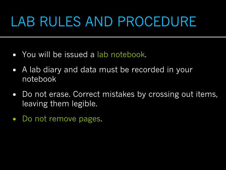
LAB RULES AND PROCEDURE
• You will be issued a lab notebook.
• A lab diary and data must be recorded in your notebook
• Do not erase. Correct mistakes by crossing out items, leaving them legible.
• Do not remove pages.

LAB SAFETY
• Some experiments use radioactive materials. You must complete the on-line radioactive handling course.
• The biggest hazards in the lab are high voltage(enough current capacity for an unpleasant shock!) and trips/falls. Never touch energized electrical components, and always look out where you are going!
• Treat the equipment with care

GRADING
• Grades will be based on the lab reports and the homework assignment.
• Labs take 2 lab periods• Turn in the lab report the Friday of the week after
the second lab session.• Exceptions are Millikan and and Compton, which
get an extraa writeup week.
• Penalty for late reports

YOUR LAB REPORT
• Include any computer-generated work (Mathcad output, etc.) in your report.
• Number and date all pages in your report.
• Refer explicitly in the text to tables, calculations, graphs.
• Be professional and neat!
• Goal of report is to inform an educated reader, not as a record of your work.
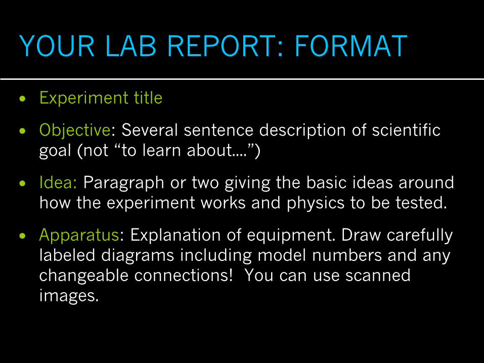
YOUR LAB REPORT: FORMAT
• Experiment title
• Objective: Several sentence description of scientific goal (not “to learn about....”)
• Idea: Paragraph or two giving the basic ideas around how the experiment works and physics to be tested.
• Apparatus: Explanation of equipment. Draw carefully labeled diagrams including model numbers and any changeable connections! You can use scanned images.

YOUR LAB REPORT: FORMAT
• Procedure:
• First person summary of process, including unexpected occurrences. What did YOU do?
• Discuss problems and how they were resolved.
• Data Analysis and Results:
• In the report inputs to all calculations must be written down explicitly.

DATA FORMAT
• STATE FORMAL RESULT ( SFR # in writeup)
- State each result as an equation
- Uncertainty rounded to 1 significant figure
- Value rounded to uncertainty
- Same power of 10 for value and uncertainty
- Units expressed
- e.g. - measured speed c = (3.44 + 0.06) • 108 m/s
• PLOTS
- Data plotted as points, theory as lines
- X,Y axes labeled with what is being plotted, with appropriate units
- Caption, explaining what is important about the plot
- Independent variable on the horizontal axis
• UNITS
- Units of all quantities used on a page immediately evident on that page
- Only one set of units in use at any given place in a report (e.g., lengths in meters)
DATA FORMAT
OK NOT SO GOOD1.41 ± 0.07 1.408 ± 0.076.7 ± 1.3 6.74 ± 1
0.1006 ± 0.002 0.1006 ± 0.004

DATA FORMAT
• STATE FORMAL RESULT ( SFR # in writeup)
- State each result as an equation
- Uncertainty rounded to 1 significant figure
- Value rounded to uncertainty
- Same power of 10 for value and uncertainty
- Units expressed
- e.g. - measured speed c = (3.44 + 0.06) • 108 m/s
• PLOTS
- Data plotted as points, theory as lines
- X,Y axes labeled with what is being plotted, with appropriate units
- Caption, explaining what is important about the plot
- Independent variable on the horizontal axis
• UNITS
- Units of all quantities used on a page immediately evident on that page
- Only one set of units in use at any given place in a report (e.g., lengths in meters)
DATA FORMAT

DATA FORMAT
• STATE FORMAL RESULT ( SFR # in writeup)
- State each result as an equation
- Uncertainty rounded to 1 significant figure
- Value rounded to uncertainty
- Same power of 10 for value and uncertainty
- Units expressed
- e.g. - measured speed c = (3.44 + 0.06) • 108 m/s
• PLOTS
- Data plotted as points, theory as lines
- X,Y axes labeled with what is being plotted, with appropriate units
- Caption, explaining what is important about the plot
- Independent variable on the horizontal axis
• UNITS
- Units of all quantities used on a page immediately evident on that page
- Only one set of units in use at any given place in a report (e.g., lengths in meters)
DATA FORMAT

YOUR LAB REPORT: FORMAT
• Conclusions
• Short discussion summarizing (restating) results.
• Compare results to accepted value: what is level of agreement based on your error estimate?
• Further comment on uncertainties: explain basis of assigning them, possible hidden errors, etc.
• Stick to scientific conclusions! No opinions, no personal comments.

GRADING CODES
• RO round off appropriately
• 1SF express uncertainty with one significant figure
• SPOT same power of ten for value and uncertainty
• SFR state final result in standard form: x = (val. ± unc.) UNITS
• AXL label axes
• (0,0) include origin in plot
• CAP no plot cption
• LABEL no axis label
• PDAP plot data as points
• UNITS express units
• SP spelling problem

UNCERTAINTY, DISCREPANCY, & ERROR
• “Uncertainty”: A remnant lack of knowledge at the end of an experiment, appearing as a result of the fact that repeated measurements of a physical quantity always give different results under conditions where the same result is expected. Uncertainties are usually evaluated using statistical analysis and expressed as some range of possible values about a mean value.. A result is meaningless without expressing its uncertainty.
• “Discrepancy”: The difference between your measured value(s) and the value(s) of the same physical quantity obtained in or calculated from other experiments or predicted by some theory.
• “Error”: Effects which systematically change measured values resulting from an experiment in a way that is not included in the analysis producing the design oif the experiment, or arise from changes of conditions unbeknownst to the experimenter are said to introduce “systematic error”.

WHY INDEPENDENT UNCERTAINTIES ADD IN QUADRATURE
INTRO - Addition in quadrature is a description in words of the Pythagorean addition c2 = a
2 + b
2 for a right
triangle, and is a characteristic of the net result of moving along orthogonal directions in a space. So we go a certain distance y north and then x east. These displacements are independent in the sense that moving north doesn’t change our east-west position: the x and y axes are orthogonal. Mathematically this shows up in the calculation of the magnitude of the net displacement vector c = x + y: This magnitude is
√c•c = √c2 = c = √(x + y)•(x + y) = √(x
2 + y
2 + 2x•y).
Since x and y are orthogonal and their displacements independent, then x•y = 0 and c = √(x2 + y
2) is given by
addition in quadrature. A similar idea applies to fluctuations contributing to a sum or product. If they are independent their net effect is obtained by addition in quadrature:
IN A SUM – Suppose a and b are some measured quantities. Measurement processes for determining a and b
give well-defined averages and uncertainties <a> ± δa and <b> ± δb. If we repeat the measurement process
for a one more time we get ai, the “i th” measurement of ai, and we can define the fluctuation δai as
δai = ai - <a>. Similarily for the j th measurement of b:
ai = <a> + δai bj = <b> + δbj
where, by definition <δai> = <δbj> = 0. If the fluctuations in a and b are independent, then the average of the
product of the fluctuations is zero: <δaiδbi> = 0 (definition of independence). The quantities √<δai2> and
√<δbj2>, always positive, are a measure of how big the fluctuations in a and b are in a single measurement.
Now we calculate the fluctuations in the sum c = a + b. Treating fluctuations like differentials, we have
<c> = <(a + b)> = <a> + <b>, and δc = δai + δbj.
<δc> = <(δai + δbj)> = 0, so the average of δc doesn’t reveal anything about the magnitude of the δc’s. To
probe this we calculate <δci2>:
<δc2> = <δai
2> + 2<δaiδbj> + <δbj
2> = <δa
2> + <δb
2>.
Since the cross term <δaiδbi> = 0 independent uncertainties in a sum add in quadrature:
δc = √<δc2> = √(<δa
2> + <δb
2>)
MULTIPLE INDEPENDENT MEASUREMENTS OF THE SAME QUANTITY – Let c = (a1 + a2 + .. + aN)/N,
where ai are independent measurements of a. Then c = 〈a〉 and <δc2> = [<δai
2> + <δa2
2> + ... +
<δaN2>]/N
2 = <δai
2>/N, where all of the cross terms <δaiδaj> = 0. Thus, after averaging N independent
measurements of a, we have:
a = 〈a〉, δa = δ〈a〉 = δai/√N, where δai is the uncertainty for a single measurement
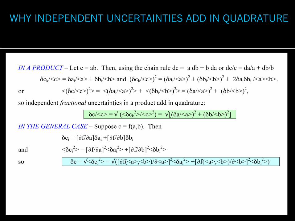
IN A PRODUCT – Let c = ab. Then, using the chain rule dc = a db + b da or dc/c = da/a + db/b
δck/<c> = δai/<a> + δbi/<b> and (δck/<c>)2 = (δai/<a>)
2 + (δbi/<b>)
2 + 2δaiδbi /<a><b>,
or <(δc/<c>)2> = <(δai/<a>)
2> + <(δbi/<b>)
2> = (δa/<a>)
2 + (δb/<b>)
2,
so independent fractional uncertainties in a product add in quadrature:
δc/<c> = √ (<δck2>/<c>
2) = √[(δa/<a>)
2 + (δb/<b>)
2]
IN THE GENERAL CASE – Suppose c = f(a,b). Then
δci = [∂f/∂a]δai +[∂f/∂b]δbi
and <δci2> = [∂f/∂a]
2<δai
2> +[∂f/∂b]
2<δbi
2>
so δc = √<δci2> = √([∂f(<a>,<b>)/∂<a>]
2<δai
2> +[∂f(<a>,<b>)/∂<b>]
2<δbi
2>)
WHY INDEPENDENT UNCERTAINTIES ADD IN QUADRATURE

WHY INDEPENDENT UNCERTAINTIES ADD IN QUADRATURE
INTRO - Addition in quadrature is a description in words of the Pythagorean addition c2 = a
2 + b
2 for a right
triangle, and is a characteristic of the net result of moving along orthogonal directions in a space. So we go a certain distance y north and then x east. These displacements are independent in the sense that moving north doesn’t change our east-west position: the x and y axes are orthogonal. Mathematically this shows up in the calculation of the magnitude of the net displacement vector c = x + y: This magnitude is
√c•c = √c2 = c = √(x + y)•(x + y) = √(x
2 + y
2 + 2x•y).
Since x and y are orthogonal and their displacements independent, then x•y = 0 and c = √(x2 + y
2) is given by
addition in quadrature. A similar idea applies to fluctuations contributing to a sum or product. If they are independent their net effect is obtained by addition in quadrature:
IN A SUM – Suppose a and b are some measured quantities. Measurement processes for determining a and b
give well-defined averages and uncertainties <a> ± δa and <b> ± δb. If we repeat the measurement process
for a one more time we get ai, the “i th” measurement of ai, and we can define the fluctuation δai as
δai = ai - <a>. Similarily for the j th measurement of b:
ai = <a> + δai bj = <b> + δbj
where, by definition <δai> = <δbj> = 0. If the fluctuations in a and b are independent, then the average of the
product of the fluctuations is zero: <δaiδbi> = 0 (definition of independence). The quantities √<δai2> and
√<δbj2>, always positive, are a measure of how big the fluctuations in a and b are in a single measurement.
Now we calculate the fluctuations in the sum c = a + b. Treating fluctuations like differentials, we have
<c> = <(a + b)> = <a> + <b>, and δc = δai + δbj.
<δc> = <(δai + δbj)> = 0, so the average of δc doesn’t reveal anything about the magnitude of the δc’s. To
probe this we calculate <δci2>:
<δc2> = <δai
2> + 2<δaiδbj> + <δbj
2> = <δa
2> + <δb
2>.
Since the cross term <δaiδbi> = 0 independent uncertainties in a sum add in quadrature:
δc = √<δc2> = √(<δa
2> + <δb
2>)
MULTIPLE INDEPENDENT MEASUREMENTS OF THE SAME QUANTITY – Let c = (a1 + a2 + .. + aN)/N,
where ai are independent measurements of a. Then c = 〈a〉 and <δc2> = [<δai
2> + <δa2
2> + ... +
<δaN2>]/N
2 = <δai
2>/N, where all of the cross terms <δaiδaj> = 0. Thus, after averaging N independent
measurements of a, we have:
a = 〈a〉, δa = δ〈a〉 = δai/√N, where δai is the uncertainty for a single measurement
IN A PRODUCT – Let c = ab. Then, using the chain rule dc = a db + b da or dc/c = da/a + db/b
δck/<c> = δai/<a> + δbi/<b> and (δck/<c>)2 = (δai/<a>)
2 + (δbi/<b>)
2 + 2δaiδbi /<a><b>,
or <(δc/<c>)2> = <(δai/<a>)
2> + <(δbi/<b>)
2> = (δa/<a>)
2 + (δb/<b>)
2,
so independent fractional uncertainties in a product add in quadrature:
δc/<c> = √ (<δck2>/<c>
2) = √[(δa/<a>)
2 + (δb/<b>)
2]
IN THE GENERAL CASE – Suppose c = f(a,b). Then
δci = [∂f/∂a]δai +[∂f/∂b]δbi
and <δci2> = [∂f/∂a]
2<δai
2> +[∂f/∂b]
2<δbi
2>
so δc = √<δci2> = √([∂f(<a>,<b>)/∂<a>]
2<δai
2> +[∂f(<a>,<b>)/∂<b>]
2<δbi
2>)
WHY INDEPENDENT UNCERTAINTIES ADD IN QUADRATURE
WHY INDEPENDENT UNCERTAINTIES ADD IN QUADRATURE
INTRO - Addition in quadrature is a description in words of the Pythagorean addition c2 = a
2 + b
2 for a right
triangle, and is a characteristic of the net result of moving along orthogonal directions in a space. So we go a certain distance y north and then x east. These displacements are independent in the sense that moving north doesn’t change our east-west position: the x and y axes are orthogonal. Mathematically this shows up in the calculation of the magnitude of the net displacement vector c = x + y: This magnitude is
√c•c = √c2 = c = √(x + y)•(x + y) = √(x
2 + y
2 + 2x•y).
Since x and y are orthogonal and their displacements independent, then x•y = 0 and c = √(x2 + y
2) is given by
addition in quadrature. A similar idea applies to fluctuations contributing to a sum or product. If they are independent their net effect is obtained by addition in quadrature:
IN A SUM – Suppose a and b are some measured quantities. Measurement processes for determining a and b
give well-defined averages and uncertainties <a> ± δa and <b> ± δb. If we repeat the measurement process
for a one more time we get ai, the “i th” measurement of ai, and we can define the fluctuation δai as
δai = ai - <a>. Similarily for the j th measurement of b:
ai = <a> + δai bj = <b> + δbj
where, by definition <δai> = <δbj> = 0. If the fluctuations in a and b are independent, then the average of the
product of the fluctuations is zero: <δaiδbi> = 0 (definition of independence). The quantities √<δai2> and
√<δbj2>, always positive, are a measure of how big the fluctuations in a and b are in a single measurement.
Now we calculate the fluctuations in the sum c = a + b. Treating fluctuations like differentials, we have
<c> = <(a + b)> = <a> + <b>, and δc = δai + δbj.
<δc> = <(δai + δbj)> = 0, so the average of δc doesn’t reveal anything about the magnitude of the δc’s. To
probe this we calculate <δci2>:
<δc2> = <δai
2> + 2<δaiδbj> + <δbj
2> = <δa
2> + <δb
2>.
Since the cross term <δaiδbi> = 0 independent uncertainties in a sum add in quadrature:
δc = √<δc2> = √(<δa
2> + <δb
2>)
MULTIPLE INDEPENDENT MEASUREMENTS OF THE SAME QUANTITY – Let c = (a1 + a2 + .. + aN)/N,
where ai are independent measurements of a. Then c = 〈a〉 and <δc2> = [<δai
2> + <δa2
2> + ... +
<δaN2>]/N
2 = <δai
2>/N, where all of the cross terms <δaiδaj> = 0. Thus, after averaging N independent
measurements of a, we have:
a = 〈a〉, δa = δ〈a〉 = δai/√N, where δai is the uncertainty for a single measurement
IN A PRODUCT – Let c = ab. Then, using the chain rule dc = a db + b da or dc/c = da/a + db/b
δck/<c> = δai/<a> + δbi/<b> and (δck/<c>)2 = (δai/<a>)
2 + (δbi/<b>)
2 + 2δaiδbi /<a><b>,
or <(δc/<c>)2> = <(δai/<a>)
2> + <(δbi/<b>)
2> = (δa/<a>)
2 + (δb/<b>)
2,
so independent fractional uncertainties in a product add in quadrature:
δc/<c> = √ (<δck2>/<c>
2) = √[(δa/<a>)
2 + (δb/<b>)
2]
IN THE GENERAL CASE – Suppose c = f(a,b). Then
δci = [∂f/∂a]δai +[∂f/∂b]δbi
and <δci2> = [∂f/∂a]
2<δai
2> +[∂f/∂b]
2<δbi
2>
so δc = √<δci2> = √([∂f(<a>,<b>)/∂<a>]
2<δai
2> +[∂f(<a>,<b>)/∂<b>]
2<δbi
2>)
WHY INDEPENDENT UNCERTAINTIES ADD IN QUADRATURE