Physics Graphing Using Excel

0.00 0.05 0.10 0.15 0.20 0.25 0.30 0.35 0.40 0.450.00

0.20

0.40

0.60

0.80

1.00

1.20

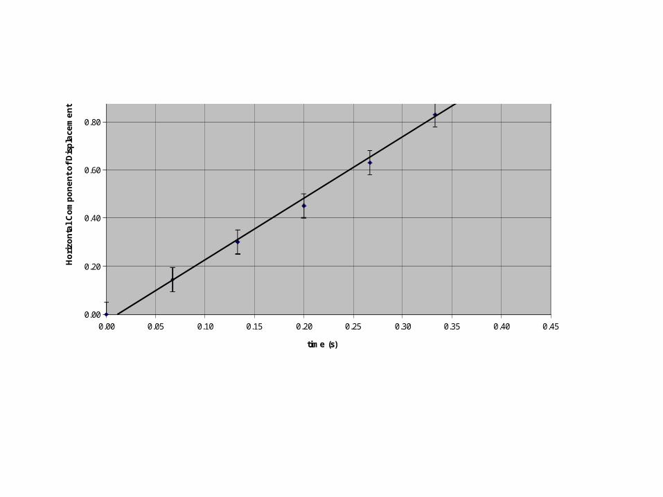
f(x) = 2.55x - 0.03

Ball Rolling off Table

time (s)

Ho

rizo

nta

l C

om

po

ne

nt

of

Dis

pla

cem

en

t (m

)

Advantages of Graphing with Spreadsheet Programs

• Can be fast. Handles lots of data and multiple calculations.

• Precise calculation of equations.

Disadvantages of Graphing with Spreadsheet Programs

• Students still need to be able to graph by hand.

• Students often do not use the correct type of graph or leave the equation in the proper format.

• Computers can not assess the importance of irregular data points.

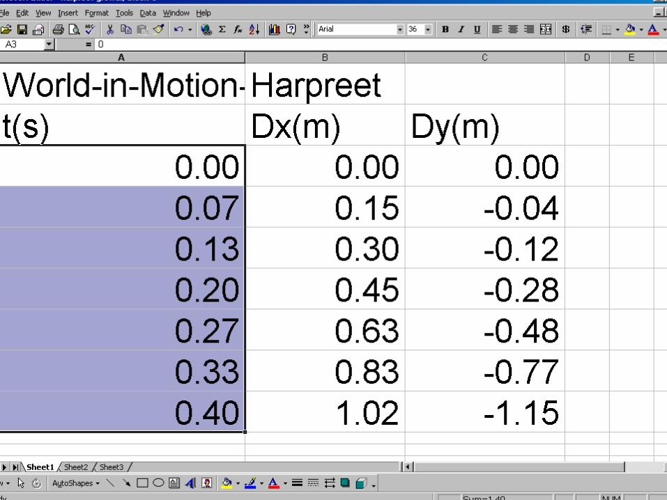
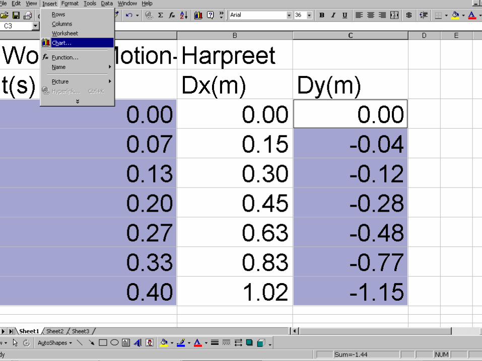
To graph data, it must be inputted into a spreadsheet program.Here is an example of data

collected by a student.

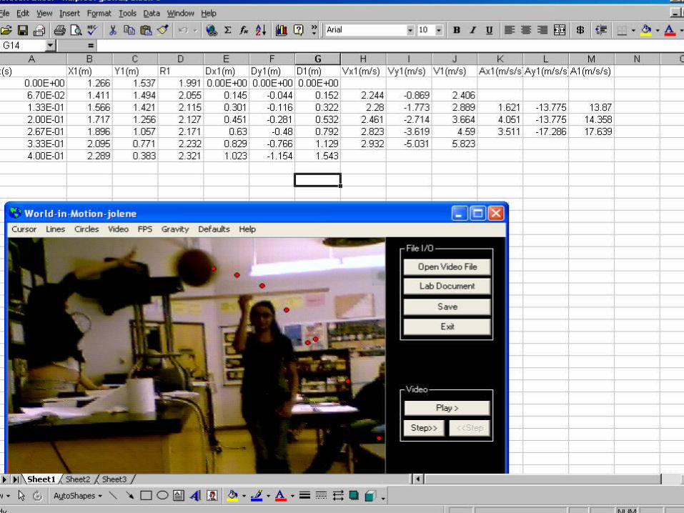
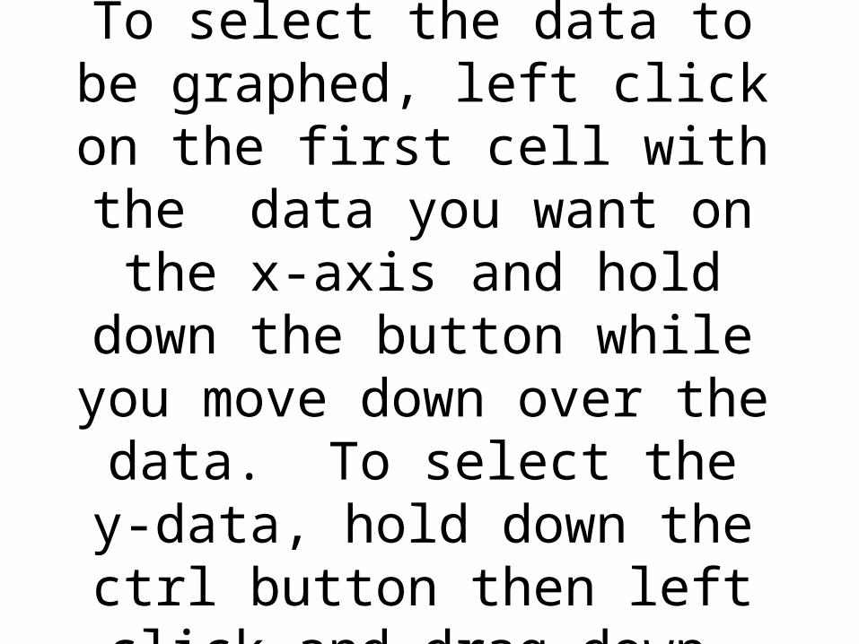
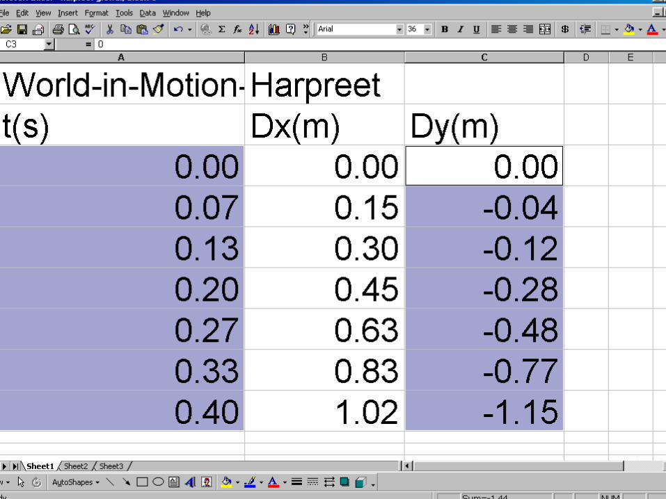
To select the data to be graphed, left click on the first cell with the data you want on the x-axis and hold down the button while you move down over the data. To

select the y-data, hold down the ctrl button then left click and

drag down.

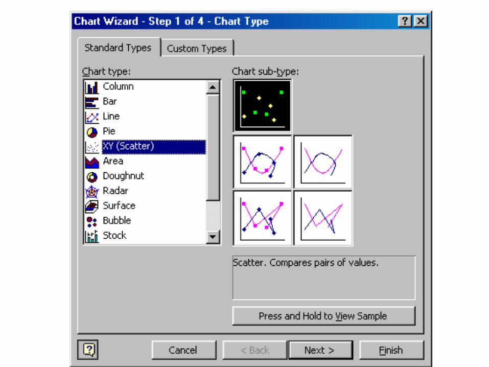
Click on Insert then Chart once the data has been selected.

Select x-y scatter plot with no lines.

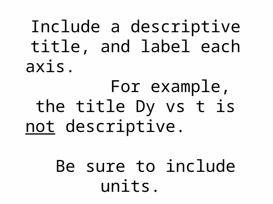
Include a descriptive title, and label each axis. For example, the title Dy vs t is

not descriptive. Be sure to include units.

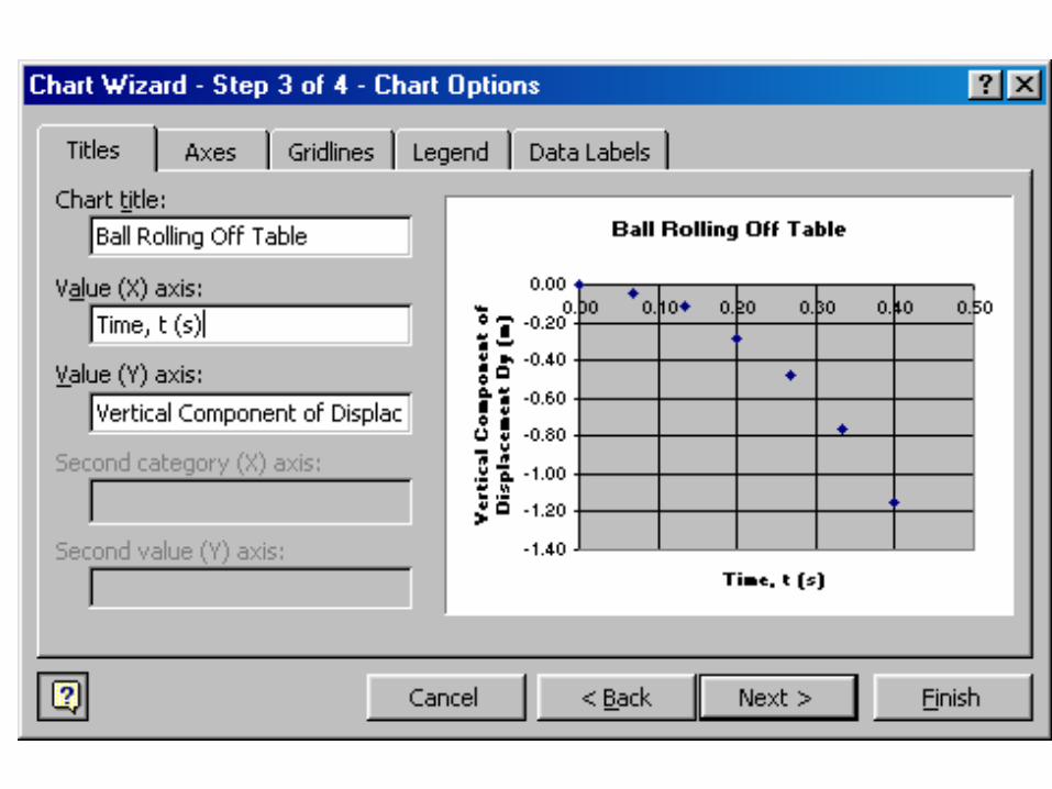
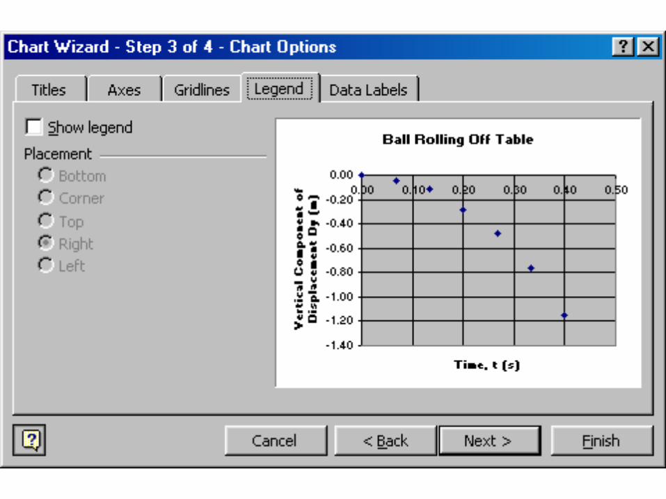
Unclick show legend

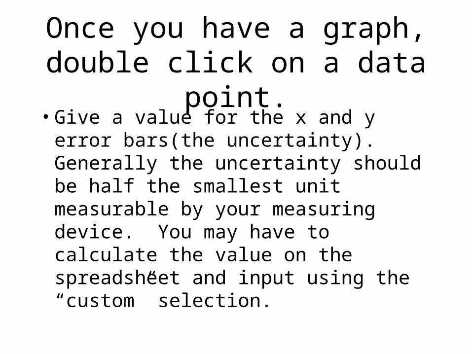
Once you have a graph, double click on a data point.

• Give a value for the x and y error bars(the uncertainty). Generally the uncertainty should be half the smallest unit measurable by your measuring device. You may have to calculate the value on the spreadsheet and input using the “custom” selection.

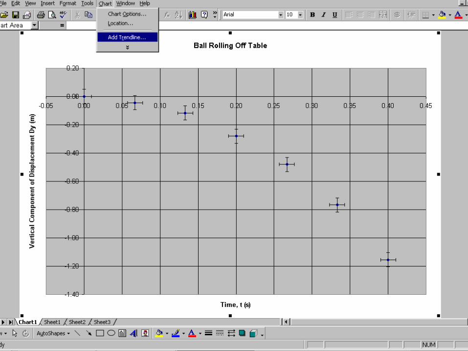
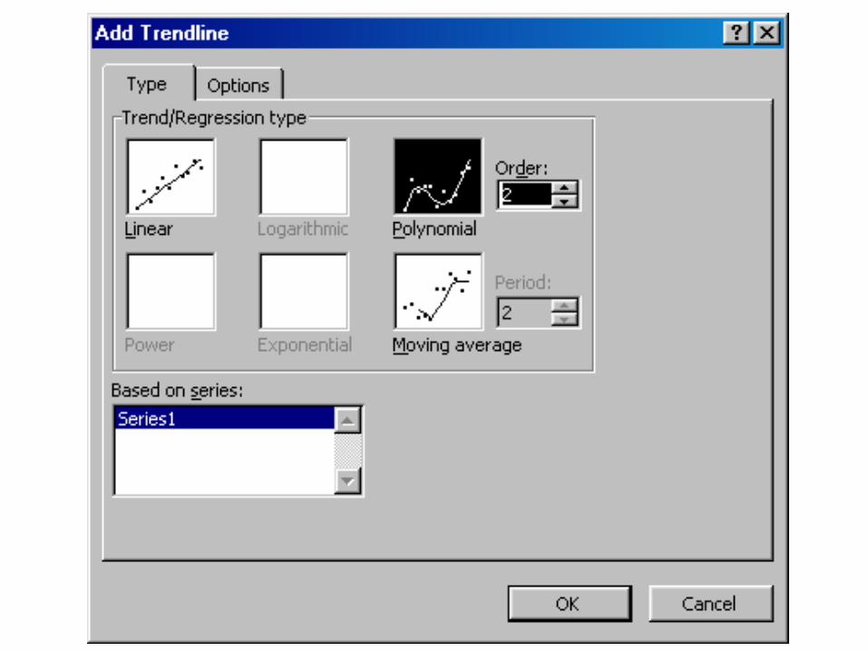
Click on Chart and add trendline.

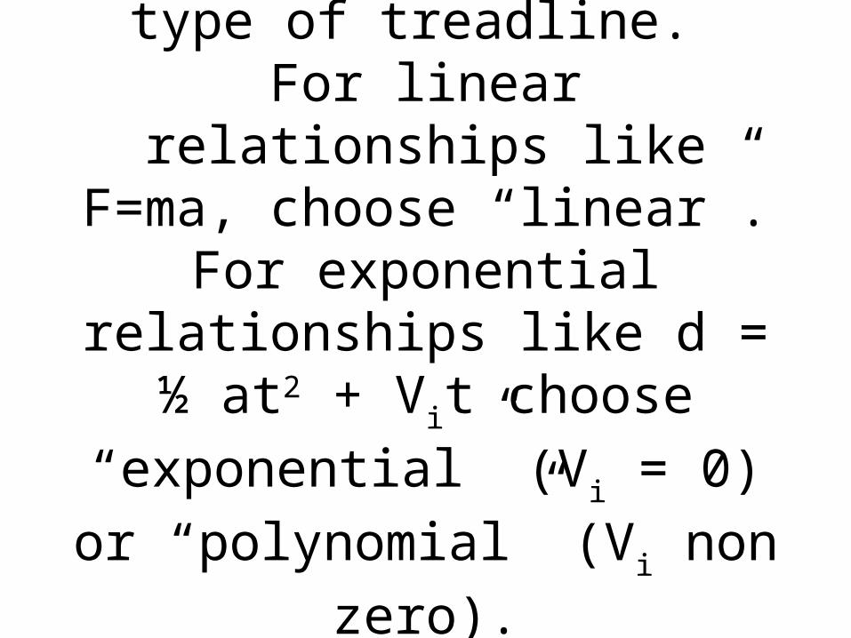
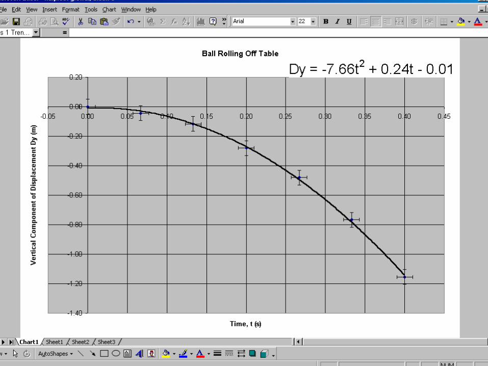
Choose the correct type of treadline. For linear relationships like F=ma, choose “linear”. For

exponential relationships like d = ½ at2 + Vit choose “exponential”

(Vi = 0) or “polynomial” (Vi non

zero).

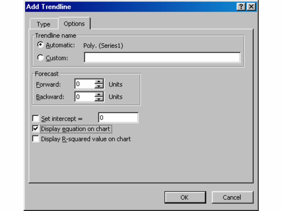
Under options select that the equation be shown on the graph.

Adjust the treadline as is appropriate for the data.

Once you have an equation, click on it. Change the variables from x and y to the quantities you are graphing, like force or position.

For polynomial equations, change the significant figures to a

reasonable number now. If the curve is very close to all the data

points you would use more significant figures than if it is far.

For linear functions, use the uncertainty of the slope to

determine precision.

Include units in your equation. Think “what are the units of the rise and run? What are the units of the slope and intercept?” If

the y variable has units of m and the x variable has units of s then the slope will have units of m/s

or ms-1 and the intercept will have units of m.

Uncertainty

Two ways to determine uncertainty of a graph:

1. LINEST function (Bonus)

2. Max-Min lines (IB required)

1. To determine the uncertainty in the slope and y-intercept.- Go back to the spreadsheet.

- Select 4 cells in a square- type =LINEST(y values, x

values,TRUE,TRUE)- press Ctrl/Shift/Enter at the

same time for PC or the command key for Macs

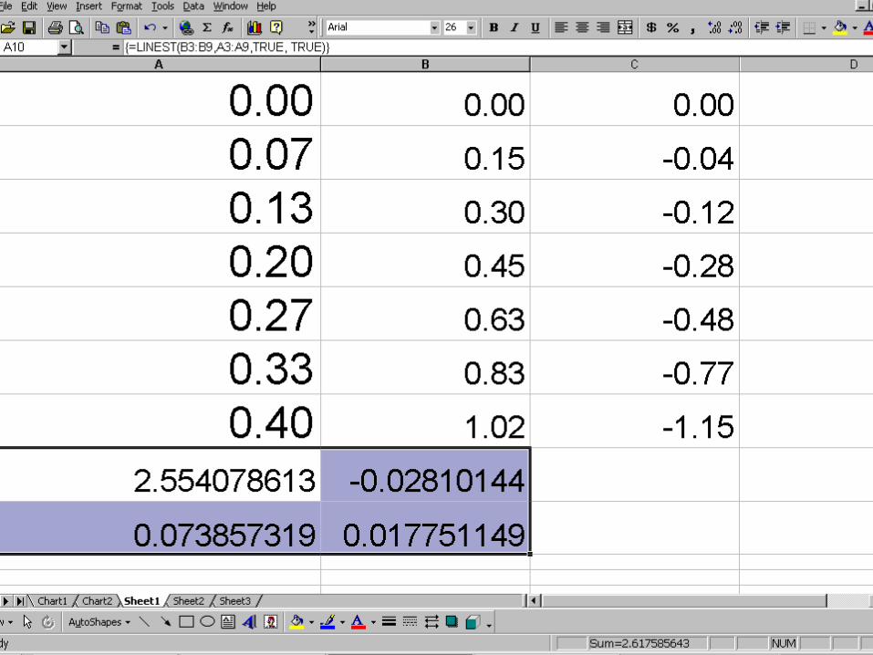
The cells correspond to the slope and y-intercept on top and the uncertainties on the bottom.

Uncertainty in slope

y-intercept

Slope

Uncertainty in y-intercept

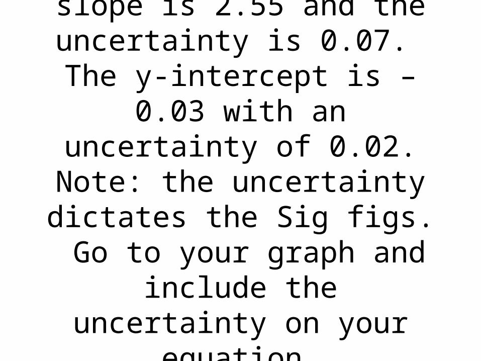
For the example the slope is 2.55 and the uncertainty is 0.07. The

y-intercept is –0.03 with an uncertainty of 0.02. Note: the

uncertainty dictates the Sig figs. Go to your graph and include the

uncertainty on your equation.

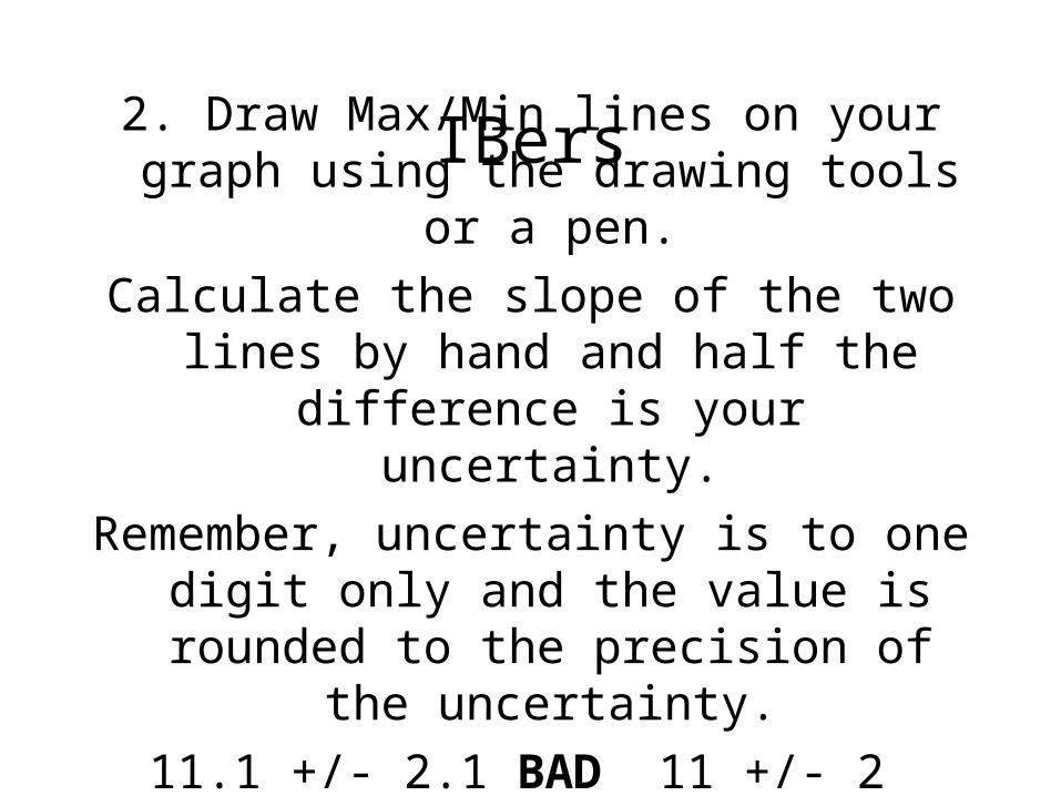
IBers

2. Draw Max/Min lines on your graph using the drawing tools or a pen.

Calculate the slope of the two lines by hand and half the difference is your uncertainty.

Remember, uncertainty is to one digit only and the value is rounded to the precision of the

uncertainty.

11.1 +/- 2.1 BAD 11 +/- 2 GOOD

Vertical Velocity of Basketball

Vy Vy = (-11+/- 2) m/s2 t + (5+/-1) m/s

(m/s)

Time (s)

0.00 0.10 0.20 0.30 0.40 0.50 0.60 0.70 0.80 0.90 1.00

-6.00

-4.00

-2.00

0.00

2.00

4.00

6.00

Check that the graph is clear with the equation easily read. If necessary, resize portions of the graph by moving a corner or side.

Copy the data and calculations into a table in your report.

Display the equations you used (copy and paste them from

Excel)

Right click on the graph and click copy then paste in your lab

report.

0.00 0.05 0.10 0.15 0.20 0.25 0.30 0.35 0.40 0.450.00

0.20

0.40

0.60

0.80

1.00

1.20

f(x) = 2.55x - 0.03

Ball Rolling off Table

time (s)

Ho

rizo

nta

l C

om

po

ne

nt

of

Dis

pla

cem

en

t (m

)

You are finished the graph!Does the graph match your hypothesis? Compare the

deviation to the uncertainty. What would account for the observed relationship? How

could you improve the experiment?