Physics Workshop: Simple mechanical, thermodynamical

1

Workshop # 38, Sharing Inspiration, Bruxelles, 2017, March, 24-27

Physics Workshop: Simple mechanical, thermodynamical, optical and electrical experiment and calculations with the TI-Nspire and LabCradle Technology

Hans Kammer, Irma Mgeladze (T3 Switzerland):

[email protected] [email protected]

Contents

1. Response Time of an Electronic Thermometer 3

2. Evaporation Heat medical Benzine or Pentane 5

3. Discharging a Capacitor with a Resistor 7

4. Pendulum 9

5. Force Plate 11

6. R-L-C-Oscillator (Oscillating Circuit) 13

7. Faraday’s Induction Law 15

8. Induction Pendulum: 2nd Harmonics Generation 17

9. Induction Signals generated by a free falling Magnet 19

10. Electric Characteristics (Bulb or LED) 21

11. Light Measurements 23

12. Velocity of Sound Measurement with two Microphones 25

13. Radioactivity Measurements 27

14. Light, Brightness and Distance: 1

- Law2r

29

mailto:[email protected]

mailto:[email protected]

2

3

1. Response Time of an Electronic Thermometer

With a Temperature sensor connected to a TI-nspire (or a TI-84) calculator, temperature data can be

measured as a function of time.

In this experiment the sensor is plunged into a Dewar Vessel of boiling water ( C97B ).

The temperature is then measured with a rate of 5 samples per second during 10 seconds (green points in Fig.

1, right).

Figure 1 Temperature Response Curve of an EasyTemp-Temperature Sensor

According to Newton’s law the temperature response function )(t (TI-nspire: 1 1f f ( x ) ) of the

sensor is delayed in respect to this Heaviside temperature step (figure 1):

1

k x

e e if ( x ) t t t e

The parameters et , it and k can be determined by “optical fitting” with three sliders (works with TI-

nspireCX CAS only): s

1 3.0k , t_e =95°C and t_i=42°C

The scatter plot of the measured values (green points in Figure 1) is in quite good accordance with the

calculated function 1f ( x ) (red curve in figure 1). Deviation may be observed in the range from 0 seconds to

0.8 seconds.

The inverse of the parameter k is the response time 1

3 3 s.k

of the temperature sensor. During this

time the temperature signal of the temperature sensor reaches 63% of its final value.

Alternatively to this type of analysis a regression analysis of environ

environ initial

k t( t )e

may be performed (for

TI-84 and for TI-nspireCX CAS).

4

Equipment : insulated e.g. Dewar vessel, boiling water,

TI-nspire CX CAS, handheld or software, Version 4.4

TI-nspire lab cradle or GoLink/EasyLink adaptor

TI-temperature probe (Vernier)

Figure 2 TI-nspire Start screen

Figure 3 Collection Setup

5

2. Evaporation Heat medical Benzine or Pentane

A precise exponential temperature decay )(t in function of time can be obtained by eva-

poration of medical benzine from a cotton fixed pad at the measuring area of an temperature sensor.

Figure 1 Measuring the evaporation cold of benzine or

pentane from an cotton pad on a temperature probe

Figure 2 Exponential Decay of the temperature on a

cotton pad moist with benzine.

Fig. 2 shows a temperature decay from 23°C to 11°C in 180 seconds.

An even faster decay can be obtained by evaporating pentane ( 125HC ) which shows a decay from 20°C

to 0°C in 150 seconds (Fig. 6).

Again this decay could be modelled by “optical fitting” of an exponential function with a constant

value added.

However this curve is analysed by a built in regression function (TI-nspire) xbay with the

variables y and x (Fig. 4). The parameters a and b are determined by an internal Gaussian least

square fit algorithm. This algorithm works however only if the zero line of the exponential growth

or decay lies at y=0 (corresponds to C0 ). The zero line of the exponential function shown in

Figure 3 is at C 2.17environ .

Figure 3 Temperature Decay from evaporating

Pentane

Figure 4 Regression Data analysis in a nspire

sreadsheet

6

If the corresponding data have to be fitted using this algorithm environ must be subtracted from the

temperature values first.

Since environ is unknown a parameter “null” which is added to the temperature data is introduced.

The procedure is shown in Figure 4:

Column A contains the time data dc01.time with one-second-steps, column B the temperature data

dc01.temp1.

Column C shows the temperatures corrected by the “null” value. In this case the “null” value is

17.2°C.

The regression is now performed in columns C and A, the results are shown at the right of Figure 4

(columns F and G).

In a corresponding geometric application (Figure 3) the regression function (solid line) and the

measured data (columns A and B) are shown (dotted line). A slider for the parameter “null” is

introduced. If this slider is animated the regression is calculated for every k-value and the results are

represented dynamically in the geometric application (Figure 4).

A “quality factor” for the correspondence between the measured data and the calculated regression

function is the regression coefficient stat.r calculated in a regression analysis.

In the best case the regression coefficient reaches a value of 0.999962 showing a very good

correspondence between experimental data and theoretical regression function.

With a regression analysis we get a numeric (quantitative) information about the accordance of the

measured data and the modelling function. This is the net advantage over the qualitative method of

“optical fitting” only.

Equipment :

- medical benzine

- Absorbent cotton or cotton pads for cosmetic use

- TI-nspire CX CAS, handheld or software, Version 4.4 or later

- TI-nspire lab cradle or GoLink/EasyLink adapter

- TI-temperature probe (Vernier)

Figure 5 TI-nspire Start screen Figure 6 Collection Setup

7

3. Discharging a Capacitor with a Resistor

An electrolytic capacitor ( μF 00001 C ) is charged with a 9-Volt-battery. Then the charging switch is

opened and the capacitor is discharged with a resistor 7004R . The voltage across the resistor (and

the capacitor) is measured with a Vernier Voltage probe which is connected to the nspire/TI-84 calculators

with an EasyLink Interface (Figures 1, 2, 3). The following instruction to perform a regression analysis is for

nspire only.

Figure 1 Discharging Circuit

Figure 2 Electrolytic Capacitor μF 7004 , Resistor

0001 and Battery (9 Volt

Figure 12 Voltage Probe and EasyLink-Interface

(Vernier)

Figure 3 Discharging and Regression Data

1. Choose “New Document” on the home screen of

the TI-Nspire (Vs. 4.4) handheld calculator.

2. Choose ”Lists & Spreadsheet”. A spreadsheet

appears (1.1)

3. Connect the voltage probe at one side (clips) to the

R-C-circuit, on the other side to the EasyLink or

lab cradle interface.

4. Connect the EasyLink mini-USB-con-nector or the

lab cradle with the TI-nspire handheld calculator.

5. The calculator automatically recognises the voltage

sensor and starts the measuring program

(DataQuest, 1.2)

6. Press the menu-key, then 1: Experiment > 7:

Collection Mode>Time Based.

7. Choose “Rate (samples/second)”, Rate “1 second”

for the time between the samples and 100 seconds

for the Experiment Duration. Press OK.

8. Charge the capacitor by shortly dipping its + pole

with the + wire of the 9 volt battery. The – pole of

the battery is connected with the – pole of the

capacitor.

9. Press to start the measurement. The

measurement data are written in the lists run1.time

and run1,potential.

10. Select the spreadsheet (ctrl <).

11. Write run1.time in the head-field of column A and

run1.potential in the head field of column B (Fig.

12).

12. Press the menu-key and select 4: Statistics>1: Stat

Calculations>A: Exponential Regression, select

run1.time for the X List and run1.potential for the

Y List. Press OK. The regression data appear in

column D (figure 3, right).

13. On the Home-Page of the calculator select a graph

page.

14. Press the menu key. Select the “Graphs”- icon .

15. Press the menu-key. Select 3; Graph Entry/Edit=>

5: Scatter Plot. Enterx run1.time

s1y run1.potential

16. Press the menu key. Select 4: Window/Zoom > 1;

Window Settings. Enter: XMin 0, XMax 100,

YMin 0 YMax 10. Press OK. The measured data

are shown (Figure 3).

Press the menu key. Select 3: Graph

8

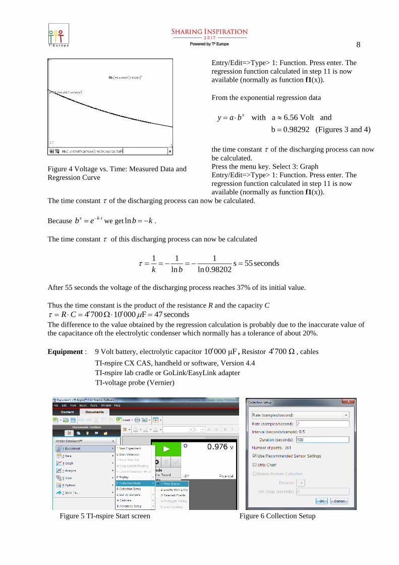
The time constant of the discharging process can now be calculated.

Because tkx eb we get kb ln .

The time constant of this discharging process can now be calculated

seconds 55s 98202.0ln

1

ln

11

bk

After 55 seconds the voltage of the discharging process reaches 37% of its initial value.

Thus the time constant is the product of the resistance R and the capacity C

seconds 47F 00001 7004 CR

The difference to the value obtained by the regression calculation is probably due to the inaccurate value of

the capacitance oft the electrolytic condenser which normally has a tolerance of about 20%.

Equipment : 9 Volt battery, electrolytic capacitor 10 000 μF , Resistor 4 700 Ω , cables


TI-nspire lab cradle or GoLink/EasyLink adapter

TI-voltage probe (Vernier)


Figure 4 Voltage vs. Time: Measured Data and

Regression Curve

Entry/Edit=>Type> 1: Function. Press enter. The

regression function calculated in step 11 is now

available (normally as function f1(x)).

From the exponential regression data

with a 6.56 Volt and

b 0.98292 (Figures 3 and 4)

xy a b

the time constant of the discharging process can now

be calculated.

Press the menu key. Select 3: Graph

Entry/Edit=>Type> 1: Function. Press enter. The

regression function calculated in step 11 is now

available (normally as function f1(x)).

9

4. Pendulum

A pendulum is a weight suspended from a pivot so it can swing freely (Figure 1).

Figure 1 Pendulum: Construction

The oscillation period T is given by Galilei’s formula g

T

2 where is the length of the pendulum

(figure 9, left) and g is the local acceleration of gravity

2s

m81.9g .

Figure 2 CBR-2 ultrasonic distance sensor

Figure 3 Oscillation measured with CBR-2

Figure 4 Results and sinusoidal Regression

The oscillation can then be described by a sinusoidal

function: T

πωtyy

2 with cos0

The movement of a pendulum is measured contactlessly

with a CBR-2 ultrasonic distance sensor (Vernier/Texas

Instruments, figure 2).

Figure 3 shows a scatter plot and figure 21 the numerical

results of the oscillations of a pendulum with a nearly

frictionless suspension (figure 1, left) (mass of the bob

500 g).

The TI-nspire-Software in this case delivers time values

(run1.time, column A), the distance (run1.position,

column B), the velocity (run1.velocity, column C) and the

acceleration (run1.acceleration, column D) every 0.05

seconds (Fig. 4).

Figures 5 and 6 show the corresponding scatter plots.

The velocity- and particularly the acceleration- plots are

much “noisier” than the original distance-plot.

The reason for deterioration of these signals is their

calculation method. The velocity is calculated by finite

10

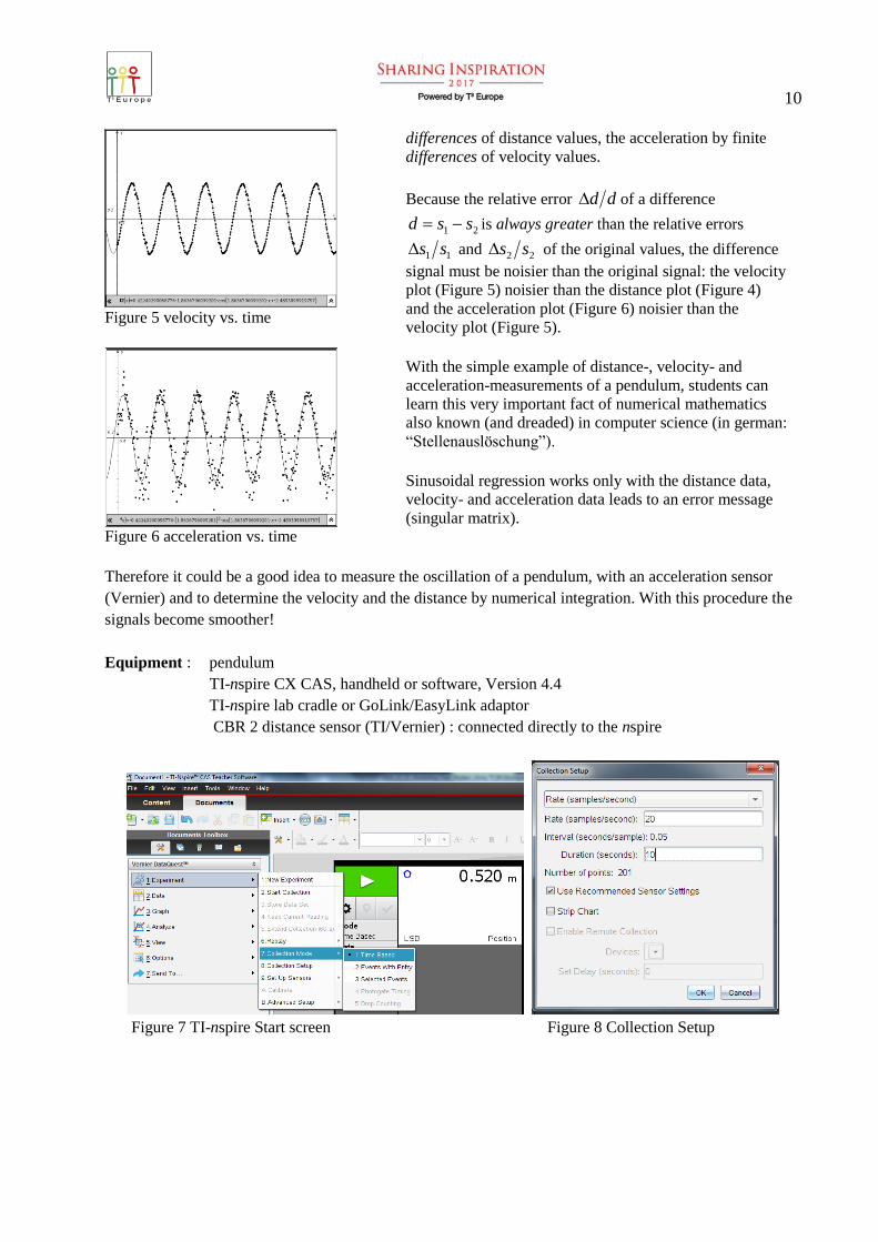
Figure 5 velocity vs. time

Figure 6 acceleration vs. time

differences of distance values, the acceleration by finite

differences of velocity values.

Because the relative error dd of a difference

21 ssd is always greater than the relative errors

11 ss and 22 ss of the original values, the difference

signal must be noisier than the original signal: the velocity

plot (Figure 5) noisier than the distance plot (Figure 4)

and the acceleration plot (Figure 6) noisier than the

velocity plot (Figure 5).

With the simple example of distance-, velocity- and

acceleration-measurements of a pendulum, students can

learn this very important fact of numerical mathematics

also known (and dreaded) in computer science (in german:

“Stellenauslöschung”).

Sinusoidal regression works only with the distance data,

velocity- and acceleration data leads to an error message

(singular matrix).

Therefore it could be a good idea to measure the oscillation of a pendulum, with an acceleration sensor

(Vernier) and to determine the velocity and the distance by numerical integration. With this procedure the

signals become smoother!

Equipment : pendulum


TI-nspire lab cradle or GoLink/EasyLink adaptor

CBR 2 distance sensor (TI/Vernier) : connected directly to the nspire


11

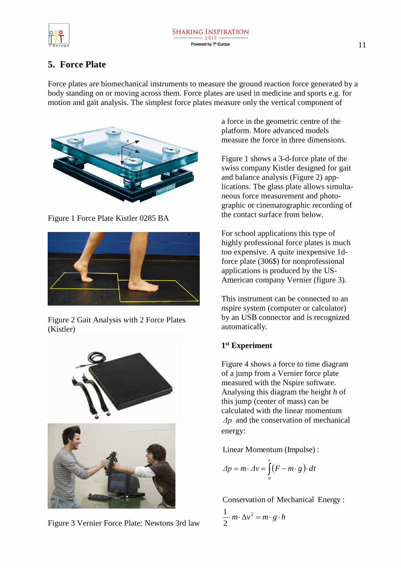
5. Force Plate

Force plates are biomechanical instruments to measure the ground reaction force generated by a

body standing on or moving across them. Force plates are used in medicine and sports e.g. for

motion and gait analysis. The simplest force plates measure only the vertical component of

Figure 1 Force Plate Kistler 0285 BA

Figure 2 Gait Analysis with 2 Force Plates

(Kistler)

Figure 3 Vernier Force Plate: Newtons 3rd law

a force in the geometric centre of the

platform. More advanced models

measure the force in three dimensions.

Figure 1 shows a 3-d-force plate of the

swiss company Kistler designed for gait

and balance analysis (Figure 2) app-

lications. The glass plate allows simulta-

neous force measurement and photo-

graphic or cinematographic recording of

the contact surface from below.

For school applications this type of

highly professional force plates is much

too expensive. A quite inexpensive 1d-

force plate (306$) for nonprofessional

applications is produced by the US-

American company Vernier (figure 3).

This instrument can be connected to an

nspire system (computer or calculator)

by an USB connector and is recognized

automatically.

1st Experiment

Figure 4 shows a force to time diagram

of a jump from a Vernier force plate

measured with the Nspire software.

Analysing this diagram the height h of

this jump (center of mass) can be

calculated with the linear momentum

Δp and the conservation of mechanical

energy:

hgmvm

dtgmFΔvmΔp

t

2

0

2

1

:Energy Mechanical ofon Conservati

:(Impulse) MomentumLinear

12

Figure 4 Jumping from the Force Plate:

Force to Time Diagram

2

20

Height of the Jump:

2 2

tF

g dtmv

hg g

Figure 5 shows some measured force

values, figure 6 the numerical

calculations with nspire. The numerical

calculation of the integral has been

performed by the trapezoidal rule

Figure 5 Measured force to time

values pairs Figure 6 Evaluation of a jump from the force plate

Equipment : Vernier Force Plate


TI-nspire lab cradle or GoLink/EasyLink adapter or

Figure 7 Force Plate : TI-nspire trigger, pretrigger and collection setup

2nd Experiment

The momentum of a free falling steel-Ball (5 kg) may be measured as an integral of the force to time

diagram. Figures 8 and 9 show the experimental setup and the evaluation of this experiment.

Figure 8 Experimental setup

Figure 9 Mathematical Evaluation

13

6. R-L-C-Oscillator (Oscillating Circuit)

A slowly oscillating electric circuit can be realised with a 500 H-/630 H-high inductivity coil (Leybold 517

011), a F40 μ capacitor (Leybold 517 021) and a 9-Volt-battery (figures 1 and 2).

Figure 1 Slowly oscillating Circuit (1 Hertz)

Figure 2 High Inductivity Coil (500 H)

and Capacitor (Leybold 517 011/021)

Figure 3 Damped Electric Oscillation

The resulting damped oscillations (figure

11) can be described by the function

teUtU tk cos0

for the voltage U(t). Again this function

can be evaluated by “optical fitting”.

Nspire has no data model for the

regression of this function.

Following Kirchhoff’s Voltage rule the sum of the three voltages across the coil, the capacitor and

the resistor must be zero:

0 :ateddifferenti 0 02

2

Inductance SelfC eCapacitanc

Ohm

LCR dt

IdL

C

I

dt

dIR

dt

dIL

C

QIRUUU

or

01

2

2

ICLdt

dI

L

R

dt

Id

This is the differential equation of a damped harmonic oscillator with the solution

14

(Thomson) 1

2 with cos and cos

0

0R0CL

and ωL

RkteRIUteItI tk

U

tk

.

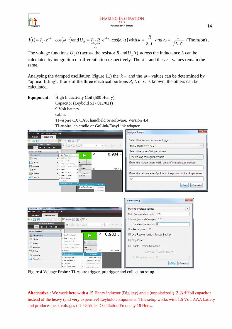
The voltage functions )(tUC across the resistor R and )(tU L across the inductance L can be

calculated by integration or differentiation respectively. The k and the values remain the

same.

Analysing the damped oscillation (figure 11) the k and the values can be determined by

“optical fitting”. If one of the three electrical portions R, L or C is known, the others can be

calculated.

Equipment : High Inductivity Coil (500 Henry)

Capacitor (Leybold 517 011/021)

9 Volt battery

cables



Figure 4 Voltage Probe : TI-nspire trigger, pretrigger and collection setup

Alternative : We work here with a 15 Henry inductor (Digikey) and a (unpolarized!) 2.2 F foil capacitor

instead of the heavy (and very expensive) Leybold components. This setup works with 1.5 Volt AAA battery

and produces peak voltages till 5 Volts. Oscillation Frequeny 18 Hertz.

15

7. Faraday’s Induction Law

If a bar magnet (length) is uniformly moved through a coil (Figure 1) a voltage is induced which depends on

the velocity of the magnet. If the magnet is not moved no voltage is induced. This voltage generated in a coil

can be measured with the voltage sensor, the EasyLink adapter and a nspire handheld calculator.

Figure 1 bar magnet in a plexiglass rod, coil

Figure 2 Voltage surge, real and idealised

The magnetic flux

dtUn

Φ ind

1

Can be calculated by a numeric integration

We get

s)(V Wb105.06.83)800,386,2( 6 Φ ,

for the left part of the signal and

6387 772 800 82 7 0 5 10 Wb (V s)Φ( , , ) . .

for the right part. The magnetic flux does not depend on the velocity which can be shown with this

experiment.

For the magnetic field we get an averge value (coil A=9 cm²)

Tesla 092.0m

sV

109

108324

6

AB

If we suppose that the distance between minimum and maximum value of the induction signal corresponds

tot he length of the bar magnet ( cm 17Δs ) the velocity of the magnet may be estimated to

s

m59.2

s 0.0656

cm 17

t

sv

Equipment : bar magnet (Frederiksen) or Neodymium-magnet (supermagnet)

plexiglass rod (length 40 cm, diameter 2 cm) ,

coil (Frederiksen Nr. 4625.25)




16


17

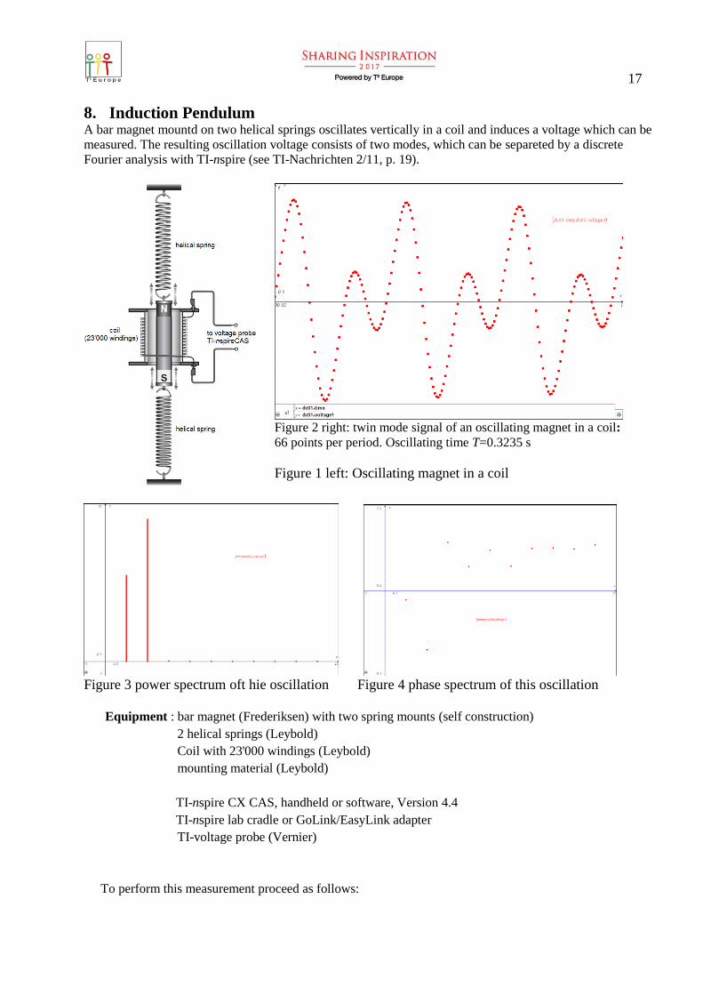
8. Induction Pendulum A bar magnet mountd on two helical springs oscillates vertically in a coil and induces a voltage which can be

measured. The resulting oscillation voltage consists of two modes, which can be separeted by a discrete

Fourier analysis with TI-nspire (see TI-Nachrichten 2/11, p. 19).

Figure 2 right: twin mode signal of an oscillating magnet in a coil:

66 points per period. Oscillating time T=0.3235 s

Figure 1 left: Oscillating magnet in a coil

Figure 3 power spectrum oft hie oscillation Figure 4 phase spectrum of this oscillation

Equipment : bar magnet (Frederiksen) with two spring mounts (self construction)

2 helical springs (Leybold)

Coil with 23'000 windings (Leybold)

mounting material (Leybold)




To perform this measurement proceed as follows:

18

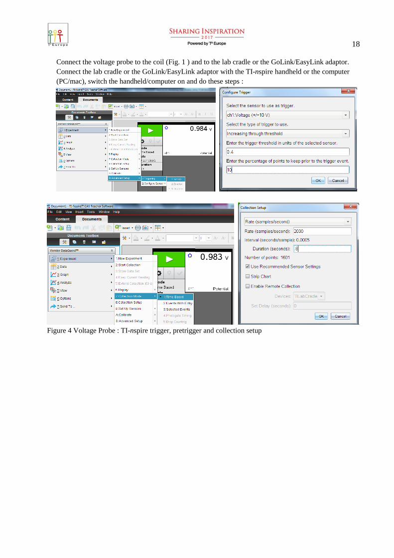
Connect the voltage probe to the coil (Fig. 1 ) and to the lab cradle or the GoLink/EasyLink adaptor.

Connect the lab cradle or the GoLink/EasyLink adaptor with the TI-nspire handheld or the computer

(PC/mac), switch the handheld/computer on and do these steps :


19

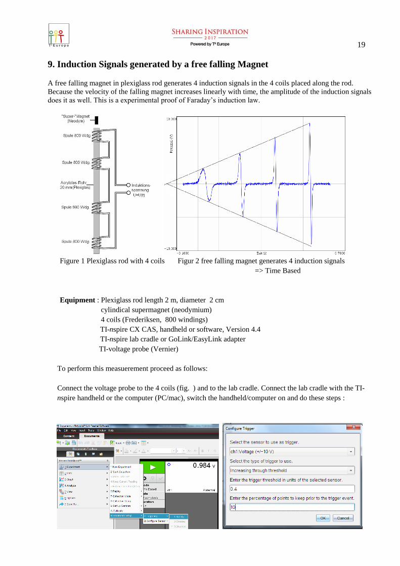
9. Induction Signals generated by a free falling Magnet

A free falling magnet in plexiglass rod generates 4 induction signals in the 4 coils placed along the rod.

Because the velocity of the falling magnet increases linearly with time, the amplitude of the induction signals

does it as well. This is a experimental proof of Faraday’s induction law.

Figure 1 Plexiglass rod with 4 coils Figur 2 free falling magnet generates 4 induction signals

=> Time Based

Equipment : Plexiglass rod length 2 m, diameter 2 cm

cylindical supermagnet (neodymium)

4 coils (Frederiksen, 800 windings)




To perform this measuerement proceed as follows:

Connect the voltage probe to the 4 coils (fig. ) and to the lab cradle. Connect the lab cradle with the TI-

nspire handheld or the computer (PC/mac), switch the handheld/computer on and do these steps :

20


With a measuring time of 0.8 seconds 2‘000 measurements are performed. The measurement starts then

automatically as soon as the falling magnet induces a voltage of .4 Volts. 10% of the range before this trigger

point will also been shown after measurement.

21

10. Electric Characteristics (Bulb or LED)

Figure 1 Circuit to measure Electric

Characteristics

Alternative: Vernier Energy Sensor VES

BTA, Variable Load VES-VL, 9 V Battery

Figure 2 Characteristics of a Filament Bulb

To measure the characteristics of an elect-

ronic/electric component, e.g. a resistor, a

diode (LED) or a filament bulb, two measu-

rements have to be done, one for the voltage,

the other for the electric current (figure 1).

A bulb has a positive temperature coefficient,

this means that the resistance at room tempe-

rature is much smaller than at its working

temperature.

The corresponding characteristics is a power

function as can be shown with 2 assumptions:

1. The resistance R of the bulb is proportional

to the absolute temperature T of the

filament TcI

UR 1 .

2. Following Stefan Boltzmann’s law the

(radiation) power is proportional to the 4th

power of the absolute temperature

bulb) theof Surface ( 4 STSIUP

6035

44

1

4

or

. U I U I

Ic

USIU

Figure 2 shows the ideal (blue) and real (green) characteristics of a bulb. The real bulb values

follow fairly well a power function, but its exponent has only a value of 0.44 (gray body) instead of

0.60 (black body).

Equipment: filament bulb 6 Volts and socket E10 or an other electronic component, e.g. a LED

regulated power supply

cables




Current probe (Vernier)

22

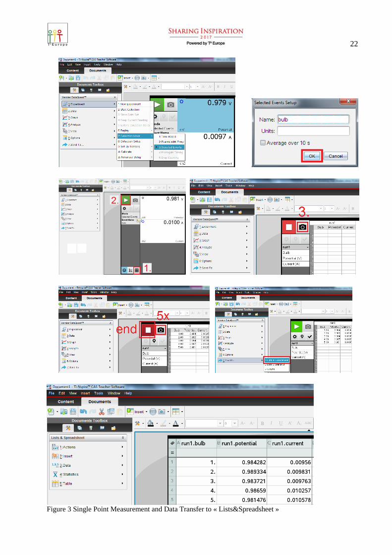
Figure 3 Single Point Measurement and Data Transfer to « Lists&Spreadsheet »

23

11. Light Measurements

Figures 1 and 2 show two light measurements near a commercial fluorescent tube (Philips Master TL5 HO

49 W /840). A 100-Hz ripple light signal (100 lux peak to peak) which is superimposed on a 3’800 lux DC

light signal can clearly be seen. Because a relatively slow light sensor is used, a part of the DC signal might

be a result of the sensors lag.

Figure 1 Light Measurement 0.1 seconds Figure 2 Light Measurement 0.03 seconds

Equipment : commercial fluorescent tube



TI-light probe (Vernier, ranges 0-6'000 lux, 0-600 lux and 0-150'000 lux)

Figure 3 Perform a time based measurement with 1201 mesurements in 0.03 seconds

24

25

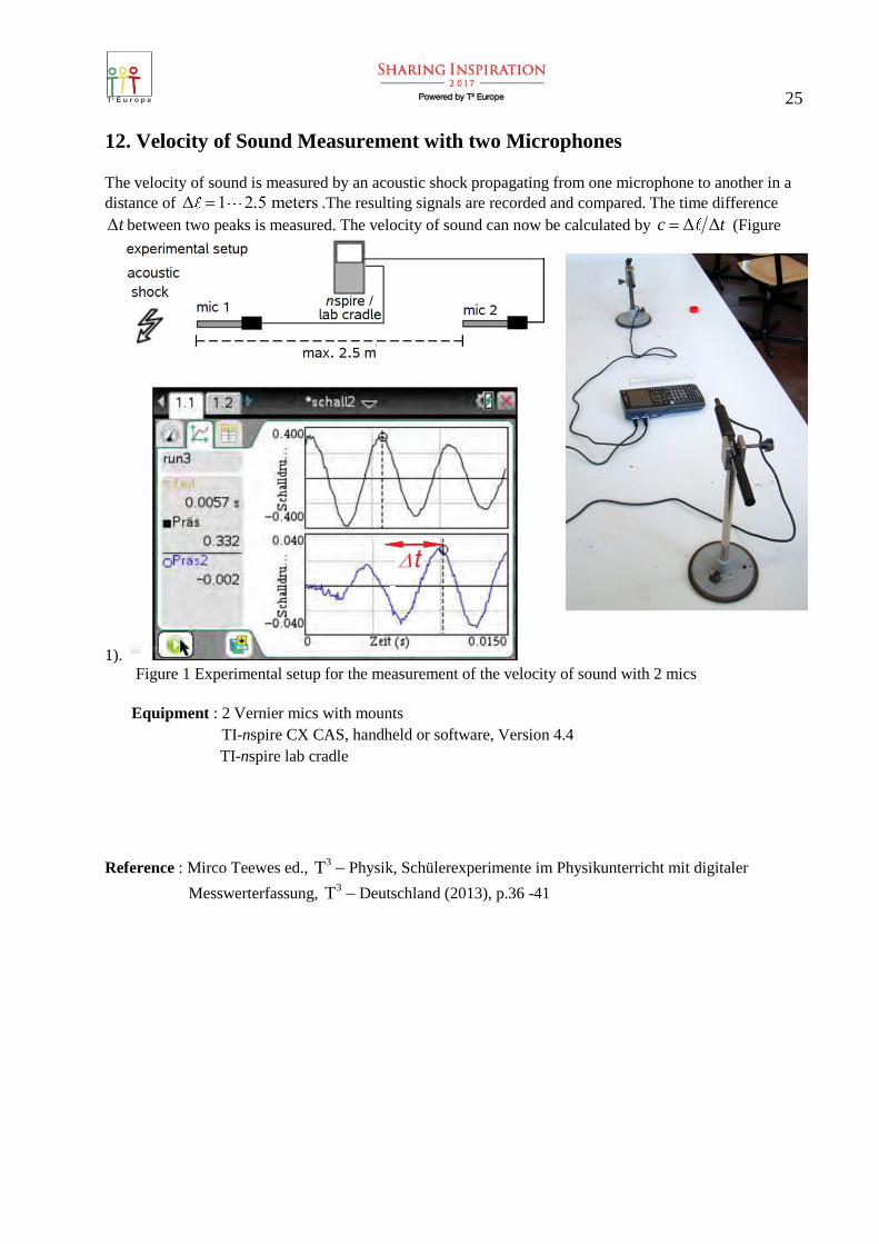
12. Velocity of Sound Measurement with two Microphones

The velocity of sound is measured by an acoustic shock propagating from one microphone to another in a

distance of Δ 1 2 5 meters. .The resulting signals are recorded and compared. The time difference

Δt between two peaks is measured. The velocity of sound can now be calculated by Δ Δc t (Figure

1). Figure 1 Experimental setup for the measurement of the velocity of sound with 2 mics

Equipment : 2 Vernier mics with mounts


TI-nspire lab cradle

Reference : Mirco Teewes ed., 3T Physik, Schülerexperimente im Physikunterricht mit digitaler

Messwerterfassung, 3T Deutschland (2013), p.36 -41

26

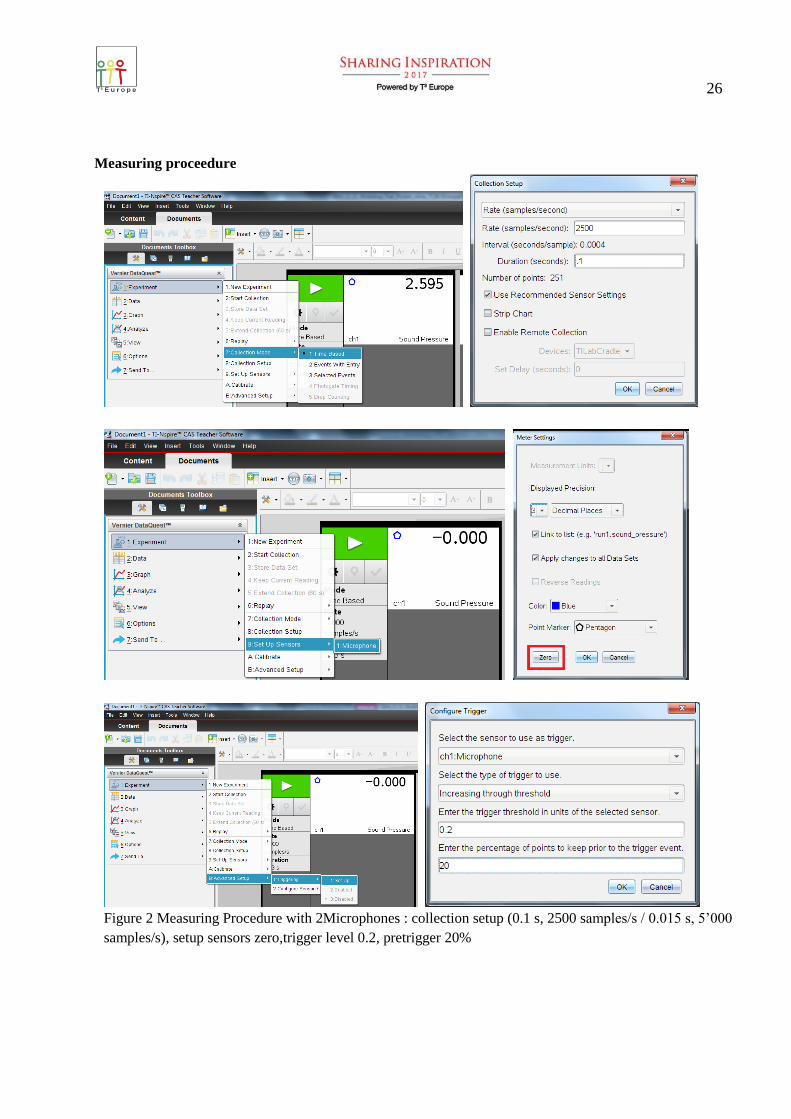
Measuring proceedure

Figure 2 Measuring Procedure with 2Microphones : collection setup (0.1 s, 2500 samples/s / 0.015 s, 5’000

samples/s), setup sensors zero,trigger level 0.2, pretrigger 20%

27

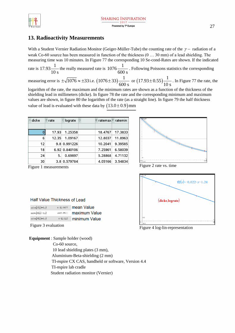
13. Radioactivity Measurements

With a Student Vernier Radiation Monitor (Geiger-Müller-Tube) the counting rate of the radiation of a

weak Co-60 source has been measured in function of the thickness (0 … 30 mm) of a lead shielding. The

measuring time was 10 minutes. In Figure 77 the corresponding 10 Se-cond-Rates are shown. If the indicated

rate is 1

17 9310 s

. the really measured rate is1

1076600 s

. Following Poissons statistics the corresponding

measuring error is 1076 33 i.e. 1

1076 33600 s

or 1

17 93 0 5510 s

. . . In Figure 77 the rate, the

logarithm of the rate, the maximum and the minimum rates are shown as a function of the thickness of the

shielding lead in millimeters (dicke). In figure 78 the rate and the corresponding minimum and maximum

values are shown, in figure 80 the logarithm of the rate (as a straight line). In figure 79 the half thickness

value of lead is evaluated with these data by 13 0 0 9 mm. .

Figure 1 measurements

Figure 3 evaluation

Figure 2 rate vs. time

Figure 4 log-lin-representation

Equipment : Sample holder (wood)

Co-60 source,

10 lead shielding plates (3 mm),

Aluminium-Beta-shielding (2 mm)


TI-nspire lab cradle

Student radiation monitor (Vernier)

28

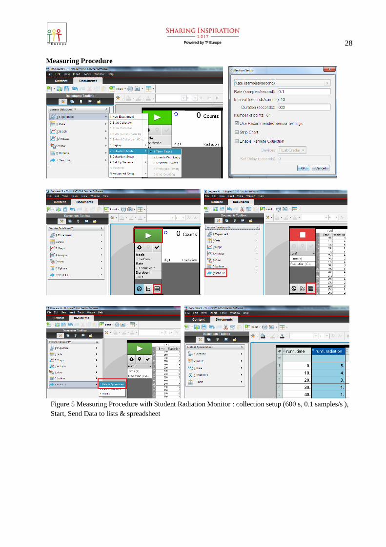
Measuring Procedure

Figure 5 Measuring Procedure with Student Radiation Monitor : collection setup (600 s, 0.1 samples/s ),

Start, Send Data to lists & spreadsheet

29

14. Light, Brightness and Distance: 1

- Law2r

In this experiment, we use a Light

Sensor to measure the illumina-

tion generated by a nearby point

light LED source as a function of

distance. We will observe how

illumination varies with distance,

and compare our results to a 21 r mathematical model.

(Components: Optics Expansion

Kit OEK, Vernier).

Figure 1 Experimental Setup:

Track, LED Light Source,

Light Sensor, Sensor Holder

Experimental Procedure

1. Manual Measurement in 1 cm-steps with the Vernier DatQuest App of the TI-nspire CX

CAS software.

2. Data Transfer (distance, illumination) to the lists&Spreadsheet App and to the graph App of

the TI-nspire CX CAS software.

3. Data evaluation with the function 2

y a x b (y illumination in Lux, x distance from light

source to light detector) and « optical » curve fitting by means of two sliders for the

parameters a and b. Best fitting with 5 23.93 10 lux cma and 1.63 cmb

Figure 2 Start “Vernier DataQuest”, single event mesasurements, start of the measurements

Figur 3 manual Measurement with “Vernier DataQuest”

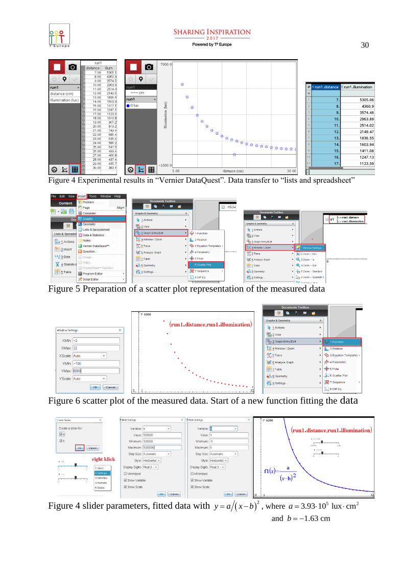
30

Figure 4 Experimental results in “Vernier DataQuest”. Data transfer to “lists and spreadsheet”

Figure 5 Preparation of a scatter plot representation of the measured data

Figure 6 scatter plot of the measured data. Start of a new function fitting the data

Figure 4 slider parameters, fitted data with

2y a x b , where 5 23.93 10 lux cma

and 1.63 cmb

31

15. Dynamics Cart and Track System with Motion Encoder (Vernier)

Figure 1 Dynamics Cart and Track System with Motion Encoder (Vernier)

The dynamics Cart and Track System with Motion Encoder (figure 1) is a new way to study

dynamics in secondary schools (Sek 2). The motion encoder is an optical position system

similar to that of shaft encoder: A double black and white fringe pattern on the track is detected

by two photore-flective sensors on the cart and is transmitted by an infrared beam to the motion

encoder recei-ver (figures 2 and 3). The digital position signals are sent to a data interface

(LabPro, Lab-quest 1 or 2, not TI nspire and labcradle!) and are evaluated by a corresponding

app, e.g. LoggerPro 3.12).

Figure 2 two fringe patterns on the track

(left),

measuring principle (right)

Figure 3 track, cart with motion detector,

motion encoder transmitter (on cart) and

detector fixed on track (left)

Linear motion with constant velocity

The motion encoder receiver will be conncted to a data logger (Lab-Pro, LabQuest), the data

logger by an USB (mini/A) to a computer (PC/Mac) with loggerPro 3.12 -Software. The Cart

with decoder electronics board is moved to its starting position, the distance measurement zeroed

(Logger Pro: Versuch => Auf null stellen => Encoderwagen). With a slowly inclined track (to

overcome friction) the cart is moved with a short kick and the measurements are started (Logger

Pro: , figure 4).

32

Figure 4 track, cart, decoder receiver. The blue Led is directed to the receiver

Figur 5 cart movement with constant velocity : position and velocity vs. Time

Linear motion with constant acceleration

The accelerated movement of the cart on a ramp (ascending slope 10 cm on the tracj length of 1

m) my be investigated in an analog way :

Figur 6 cart movement with constant acceleration: position vs. Time

Figur 7 cart muvement with constant acceleration: velocity vs. Time

33

16. Light Diffraction Apparatus (Vernier)

Figure 1 Vernier «Diffraction Apparatus» DAK

With this diffraction apparatus

diffraction patterns of a variety of

slits, double and multiple slits with

laser light (635 nm and 532 nm)

may be investigated and measured.

The high precision slits, made by

evaporation technique, allow quan-

titative evaluation of the diffraction

patterns and the comparison of the

measurements with the intensity-

function 2 2sin ( )x x of Fraunhofer’s theory. Figures 1 and 2 show the experimental setup. The light

intensity is measured with a high sensitivity light sensor the position with a linear position sensor. This

position sensor uses a precision optical encoder to measure translation with better than 50 micron

resolution. Since it is optically based, without gears or racks, it has zero backlash.

Figure 2 Experimental Setup. Left: position and intensity sensors , Right: slits-slider and laser

In order to provide excellent spatial resolution, a selectable entrance aperture (0.1 mm, 0.2 mm, 0,3

mm, 0.5 mm, 1.0 mm, 1.5 mm, open and closed) restricts the width of the pattern viewed by the

High Sensitivity Light Sensor. The light sensor has three ranges, allowing the study of fine details

or gross features of patterns.

A measurement is performed by choosing first the appropriate entrance aperture (typically 0.3 mm)

and the slit and by directing the (red or green) laser beam to the slit and the entrance aperture and

the high sensitivity light sensor. The digital position and the analog light signals are sent to a data

interface (LabPro, Lab-quest 1 or 2, not TI nspire and labcradle!) and are evaluated by a

corresponding app, e.g. LoggerPro 3.12). The measurements are started (Logger Pro: ).

The position sensor is then moved slowly over a distance of 15 cm in 30 seconds whereby the

diffraction pattern is detected digitally.

Figure 3 measurement of a diffraction (double Slit, b=0.08 mm, a=0,5 mm) with LoggerPro 3.12

34

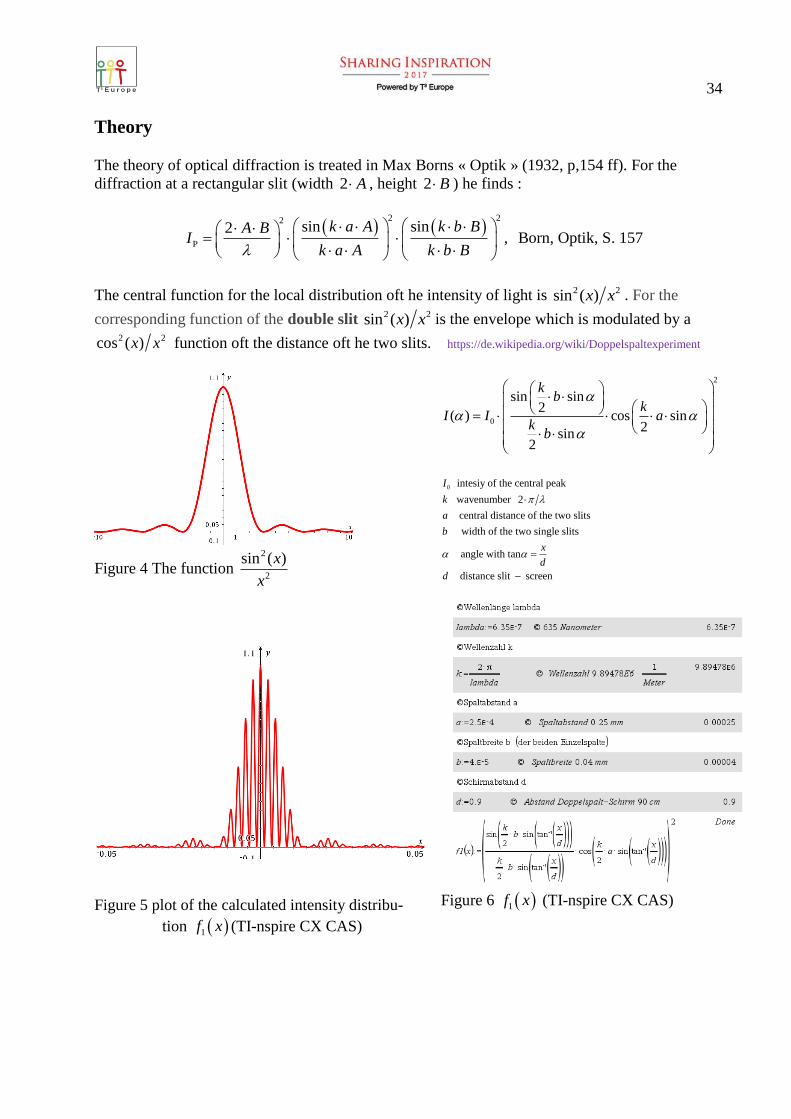
Theory

The theory of optical diffraction is treated in Max Borns « Optik » (1932, p,154 ff). For the

diffraction at a rectangular slit (width 2 A , height 2 B ) he finds :

2 22

P

sin sin2, Born, Optik, S. 157

k a A k b BA BI

k a A k b B

The central function for the local distribution oft he intensity of light is 2 2sin ( )x x . For the

corresponding function of the double slit 2 2sin ( )x x is the envelope which is modulated by a 2 2cos ( )x x function oft the distance oft he two slits. https://de.wikipedia.org/wiki/Doppelspaltexperiment

Figure 4 The function 2

2

sin ( )x

x

Figure 5 plot of the calculated intensity distribu-

tion 1f x (TI-nspire CX CAS)

2

0

sin sin2

( ) cos sin2

sin2

kb

kI I a

kb

0 intesiy of the central peak

wavenumber 2

central distance of the two slits

width of the two single slits

angle with tan

distance slit screen

I

k

a

b

x

d

d

Figure 6 1f x (TI-nspire CX CAS)

35

1 1 2 2

3 3 4 4

5 5 6 6

7 7 8 8

9 9 10 10

11 11 12 13

14 14 15 15

36

16 16 17 17

Documents

Physics Workshop: Simple mechanical, thermodynamical