pile, installation process, numerical modelling, material ... · 88 elements geotechnical codes which incorporates Lagrangian formulations are unsuitable to 89 simulate these types

Draft

Numerical Simulation of the Installation of Jacked Piles in

Sand with the Material Point Method

Journal: Canadian Geotechnical Journal

Manuscript ID cgj-2016-0455.R3

Manuscript Type: Article

Date Submitted by the Author: 02-May-2017

Complete List of Authors: Lorenzo, Raydel; Universidade Federal do Tocantins, Civil Engineering Cunha, Renato; University of Brasília, Civil and Environmental Engineering Cordao-Neto, Manoel Porfirio; University of Brasilia Nairn, John; Oregon State University, Wood Science and Engineering

Keyword: pile, installation process, numerical modelling, material point method, subloading cam clay

https://mc06.manuscriptcentral.com/cgj-pubs

Canadian Geotechnical Journal

Draft

1

Numerical Simulation of the Installation of Jacked Piles in Sand with the Material Point 1

Method 2

Lorenzo R.*, da Cunha R. P.

**, Cordão Neto M. P.

**, Nairn J. A.

*** 3

*Professor at Civil Engineer Department 4

Federal University of Tocantins 5

web page: www.uft.edu.br/engenhariacivil 6

email: [email protected] 7

**Professor at the Geotechnical Post-Graduation Program 8

University of Brasilia 9

Campus Darcy Ribeiro, SG12 Brasilia, Brasil 10

web page: www.geotecnia.unb.br 11

12

***Professor at Wood Science and Engineering 13

Oregon State University 14

Corvallis, Or 97330, USA 15

web page: http://www.forestry.oregonstate.edu 16

17

18

19

20

21

22

23

24

Page 1 of 55



Draft

2

Abstract 25

Pile installation has a great impact on the subsequent mechanical pile response. It, however, 26

is not routinely incorporated in the numerical analyses of deep foundations in sand. Some of 27

the difficulties associated with the simulation of the installation process are related to the fact 28

that large deformations and distortions will eventually appear. The Finite Element Method is 29

not well suited to solve problems of this nature. Hence, an alternative procedure is tested 30

herein, by using the Material Point Method to simulate the installation of statically jacked or 31

pushed-in type piles, which has successfully demonstrated its capacity to deal with this 32

simulation. Two constitutive models were also tested, i.e. the Modified Cam Clay (MCC) and 33

the Subloading Cam Clay (SubCam), allowing a clear perception of the great advantage to 34

consider the soil with the SubCam model. The simulations have indeed reproduced some of 35

the important features of the pile installation process, as the radial stress acting around the 36

pile´s shaft or the shaft´s lateral capacity, among other issues. The numerical results were 37

additionally compared to known (semi empirical) methods to derive the lateral capacity of the 38

shaft, with a good and practical outcome. 39

40

Keywords: pile installation process, numerical modelling, material point method, subloading 41

cam clay, granular soil. 42

43

44

45

46

47

Page 2 of 55



Draft

3

Introduction 48

In Brazil, typical calculations for the pile foundation capacity are done via empirical 49

techniques. The effects that pile installation introduce to its capacity have already been 50

studied by Randolph et al. (1979) by using the Cavity Expansion Method. These effects can 51

produce changes in the properties and state of the soil, modifications on the lateral and 52

vertical stresses and therefore changes in the capacity and the stiffness of the pile-soil system. 53

Although this problem is well known, there is still a great deal of empiricism in the 54

estimations of pile installation effects, hence some further experience is needed to do an 55

accurate evaluation of changes in pile load capacity (Doherty and Gavin 2011). Pile 56

installation effects are particularly important for displacement piles, where the soil is radially 57

and vertically displaced creating a total displaced volume of soil of, at least, the nominal 58

volume of the pile. This displacement invariably causes large variations in soil stresses 59

around its shaft. According to Randolph (2003) any scientific approach to predict the shaft 60

capacity of a driven (as well as a pushed-in type) pile must consider the changes that occur 61

during installation, as well as equalizations of excess pore pressures in the soil and the 62

loading phases of the foundation. 63

Some empirical equations have already been proposed to account for the installation effects 64

of driven piles. Figure 1 presents the idealized exponential profile of shaft’s friction proposed 65

by Randolph et al. (1994). Based in this assumption the authors obtained Eq. (1) to estimate 66

the ratio between the horizontal effective stress after the installation of the pile ( )rσ′ and the 67

initial vertical effective stress ( )Voσ′ . This ratio is expressed as a coefficient K that varies 68

along the depth, as follows: 69

( ) ( ) ( )min max min e

h dK z K K K

µ−= + − (1) 70

Page 3 of 55



Draft

4

maxK can be estimated as 2% of the normalized cone resistance c Vq σ ′ for closed-ended pile 71

and 1% of c Vq σ ′ for open-ended piles (Fleming et al. 2009).

minK can be linked to the active 72

earth pressure coefficient, µ is a coefficient that controls the rate at which the maximum shaft 73

friction is degraded, L is the embedded length of the pile and h is the vertical distance from 74

the pile tip to the point of analyses at a depth z. 75

More recently Jardine et al. (2005) suggest an equation to directly calculate the horizontal 76

effective stress after the installation of a driven pile in sand, as follows: 77

( ) ( )0.13 0.380.029r c zo aq P h Rσ σ

−′ ′= (2) 78

Where aP is the atmospheric pressure and R the radius of the pile. 79

In general, the effects that the installation of piles introduce are intrinsically related to the 80

displacement of the soil around the pile; the modification of the soil´s properties, and the 81

generation of pore pressures (Gue 1984; Randolph et al. 1979; Slatter 2000). Phenomena 82

such as “friction fatigue” and aging that affect the behavior of the pile are extremely 83

influenced by the installations process (White and Lehane 2004; Zhang and Wang 2009; 84

Zhang and Wang 2014). 85

For complex geotechnical conditions or initial conditions that are different from the 86

empirically based methods, numerical modeling is mandatory. However, generic finite 87

elements geotechnical codes which incorporates Lagrangian formulations are unsuitable to 88

simulate these types of problems (Dijkstra et al. 2011), given the large strains and 89

deformations that occur around driven piles during the installation process. Numerical 90

methods that combine the Lagrangian and Eulerian descriptions of motion have been 91

preferred for the simulations of penetration problems (Dijkstra et al. 2011; Nguyen et al. 92

2014; Sheng et al. 2009; Zhang et al. 2014). Very recently the MPM has also been used to 93

Page 4 of 55



Draft

5

simulate pile installation phenomena. Phuong et al. (2014, 2016) used the MPM with a 94

special approach called a Moving Mesh to simulate a pushed-in pile installation in a 95

hypoplastic soil model. Hamad (2016) used an extended version of the MPM knowns as 96

Convected Particle Domain Interpolation (CPDI) for dynamically installation of a driven pile 97

also in a hypolastic soil model. 98

In the present paper, simulations of the installation process of jacked (pushed-in) piles were 99

done using the Material Point Method (MPM) and two critical state models. For all numerical 100

simulations, the NairnMPM code where no water pressure generation is allowed or 101

considered was used (Nairn 2011). In the end, a parametric analysis is done to evaluate the 102

influence of some key parameters on the derived response of the soil. Finally, an evaluation 103

of considering, or not, the pile installation process in the assessment of the ultimate shaft 104

resistance is done. 105

Material Point Method and Constitutive models 106

Brief description of MPM 107

In recent years, the finite element method (FEM) has become the standard tool for solving 108

problems in solid mechanics. Nevertheless, this method, in its traditional Lagrangian 109

formulation, is not suitable for the analysis of large deformation problems (Bardenhagen et 110

al. 2000; Wieckowski 2004). According to Beuth et al. (2007) by using this formulation great 111

distortions of the mesh can occur and remeshing may be needed. 112

To solve issues with the FEM in the simulation of large deformation problems, meshless 113

methods have been developed. For these methods, the generation of the mathematical space 114

(where the governing equations of the problem will be solved) reduces to the generation of 115

material points and its distribution, without any fixed connectivity between them, as in the 116

Page 5 of 55



Draft

6

FEM. Examples of such methods are the discrete element method (DEM), the smooth particle 117

hydrodynamics (SPH) and the particle in cell method (PIC) (Zabala 2010). 118

The Material Point Method is a type of PIC (Sulsky et al. 1994). This method combines ideas 119

and procedures of the particle methods and FEM together, and uses the potential of the 120

Lagrangian and Eulerian descriptions of kinematics. With the MPM, a body is modeled as a 121

group of Lagrangian particles. These particles transport the state and other variables needed 122

to solve the problem’s governing equations (e.g. momentum equations). The variables 123

(defined by such equations) are interpolated from particles to the nodes of a fixed mesh (as in 124

FEM) in which the governing equations are solved. After obtaining the overall solution, it is 125

interpolated back to the particles, allowing the state variables and positions to be updated. 126

This procedure is repeated along the whole time domain of the problem, so that, in this way, 127

the fixed mesh has no distortion (Bardenhagen and Kober 2004; Solowski and Sloan 2015). 128

In the last decade, a generalization to the MPM was done to mitigate numerical noise that 129

arises when particles cross from one cell to another. This method is known as the Generalized 130

Interpolation Material Point (GIMP) and it was introduced by Bardenhagen and Kober 131

(2004). New interpolation shape functions are introduced over each particle’s domain, which 132

may intersect several cells of the mesh, allowing the tracking of any particle when it goes out 133

of its original cell domain. More recently, a modification was introduced to the GIMP method 134

to solve problems that appear when large distortions and tensions occur. This new technique 135

is known as the Convected Particle Domain Interpolation (CPDI) as presented by Sadeghirad 136

et al. (2011). 137

The numerical code used in the present paper was developed by Nairn (2011) and is denoted 138

as NairnMPM. It allows the establishment of dynamic 2D and 3D analyses, as well as the use 139

of GIMP and CPDI methods. It also allows the addition of a Coulomb friction between 140

Page 6 of 55



Draft

7

bodies with two contact conditions, one proposed by Bardenhagen et al. (2000), necessary but 141

not sufficient to define the contact, and other proposed by Lemiale et al. (2010) that 142

complements the first one. For the simulations done in this research, some models were run 143

using both CPDI and GIMP versions of the MPM. Negligible differences in the results were 144

observed when using GIMP or CPDI versions. The CPDI version however consumed more 145

computational time. Thus, for all the simulations the GIMP method was used. 146

Brief description of Modified Cam Clay model 147

The elastoplastic theory is the largest source of constitutive models that are applied nowadays 148

to geomechanics (Zdravkovic and Carter 2008). One of the most used models based on 149

critical state is the Modified Cam Clay (MCC) model. This model is relatively simple and 150

captures reasonably well the main features of the behavior of normally consolidated clays. 151

Only a few parameters are needed and they are easy to be assessed. 152

The plastic multiplier for this model is expressed as: 153

: :

: :

T

e

pT T

e

p

v

fD d

f g f fD tr

εσ

λ

σ σ σε

∂∂

= ∂ ∂ ∂ ∂ − ∂ ∂ ∂∂

% %% %%%%%

%%%%% % %% % %

(3) 154

where p

vε is the plastic volume deformation, ( )tr represent the trace of the entity, eD the 155

elastic constitutive tensor, σ is the Cauchy stress tensor, f and g are respectively the yield and 156

plastic potential. 157

In spite the fact that the MCC was developed based on tests on clays, very loose and dense 158

sands also show qualitatively the same stress–strain–dilatancy characteristics as those of 159

normally and over consolidated clays (Nakai 2013). Thus, for problems where some specific 160

Page 7 of 55



Draft

8

characteristics of sands, such as liquefaction and particle breakage, are not substantially 161

important, the MCC can be used. 162

Nevertheless this model is unable to describe some important features of the soil behavior, 163

such as a positive dilatancy during strain hardening, or cyclic loading, or the influence of 164

both density and confining pressure on the soil’s deformation and strength characteristics 165

(Pedroso et al. 2005). 166

Subloading Cam Clay model 167

In its original form, the MCC model yields a non-linear elastic behavior under both unloading 168

and reloading paths for overconsolidated clays. However, “real” soils show elastoplastic 169

behavior even in the overconsolidated region (Hashiguchi and Ueno 1977; Nakai 2013). To 170

solve this misconception Hashiguchi and Ueno (1977) introduced the subloading surface 171

concept. This is basically a new surface internal to the yield one which has the same 172

geometrical form. In the stress space, the actual stress point is always on the subloading 173

surface and the evolution of this surface depends on the elastoplastic transition. The models 174

introduced with this concept are known as surface loading type models (Hira et al. 2006). In 175

this way, the yield surface is no longer used to separate elastic and elastoplastic regions. The 176

yield surface acts as a bounding surface and the distance between the yield and the 177

subloading surface defines a parameter that affects the value of the plastic multiplier. When 178

the yield and subloading surfaces match, the plastic multiplier will have the same value as if 179

calculated by the original MCC model, nevertheless, if they do not match, the plastic 180

multiplier will have a lower value that depends of the distance between the surfaces. 181

The incorporation of the subloading concept to a particular model introduced a new internal 182

variable (ρ) that defines the size of the subloading surface. In the case of sands, it is a 183

measure of the relative density, whereas in the case of clays, it is associated with the 184

Page 8 of 55



Draft

9

overconsolidation ratio (see Figure 2). The introduction of this variable to a conventional 185

elastoplastic model improves its capacity to reproduce the cyclic behavior of materials, and 186

the transition from elastic to elastoplastic states (Nakai 2013). 187

The SubCam model proposed by Pedroso (2006) introduces the subloading surface to the 188

well-known MCC. This model considers the influence of density and confining pressure on 189

the deformation and strength of soils and according to Farias et al. (2005); Farias et al. 190

(2009); and Pedroso et al. (2005) it can be used for clay and sands. The SubCam model has 191

been successfully used in finite elements codes for the simulation of sand problems (Farias et 192

al. 2005). 193

The new internal variable ρ becomes null when the stress path reaches the normal 194

compression line (NCL). It is therefore related to the overconsolidation ratio as follows: 195

( ) 0

0

lnp

zρ λ κ

= −

(4) 196

where 0z is the interception of the subloading surface with the isotropic compression axis, λ 197

is the slope of the normal compression line in the ln p′ versus void ratio (e) space, κ is the 198

slope of the unloading-reloading line in the same space ( ln p′ vs. e), and 0p is the pre-199

consolidation stress. 200

The same flow rule defined for the yield surface in the MCC is used in the SubCam. On the 201

other hand, for the subloading surface another flow rule is defined that considers a strain 202

variable known as the subloading plastic strain ( )( )p SL

vε . 203

( )( )

( )( )0 0

0

1 p SLp

v v

z edz d dε ε

λ κ

+= +

− (5) 204

According to Nakai and Hinokio (2004), ( )p SL

vε can be obtained as follows: 205

Page 9 of 55



Draft

10

( )

( )( )

01

p SL

v p

G

e p

ρρε λ

−= =

+ (6) 206

where ( )Gρ is a function that controls the degradation of ρ. This function was proposed by 207

Nakai and Hinokio (2004) to be ( ) 2G aρ ρ= . The parameter ( )a is a unique and new parameter 208

added by this model to the MCC model, and can be obtained by a calibration procedure with 209

oedometric tests. The value of a influence in the curvature of the oedometric path near the 210

preconsolidation stress (Nakai 2013). 211

Considering the consistency condition and ( )p SL

vε , the plastic multiplier for the SubCam model 212

can be obtained as: 213

( )

( )0 0

0

: :

1: :

T

e

SL

pT T

e

fD d

z ef g f fD tr L

z

εσ

λ

σ σ λ κ σ

∂∂

= +∂ ∂ ∂ ∂ − +

∂ ∂ ∂ − ∂

% %% %%%%%

%%%%% % %% % %

(7) 214

( )( )

2

0

0 0

ln1

p

e zL a

p

λ κ − + = (8) 215

where L is an auxiliary function. 216

The consistency condition, in this case, is applied to the subloading surface and not to the 217

yield surface as normally done in elastoplastic models. 218

If the derivative related to the internal variables are replaced in equations (3) and (7), the 219

plastic multipliers are expressed as: 220

( )

( )0 02

: :

1: :

T

e

pT T

e

fD d

p ef g fD M p tr

εσ

λ

σ σ λ κ σ

∂∂

= +∂ ∂ ∂

+ ∂ ∂ − ∂

% %% %%%%%

%%%%% % %% % %

(9) 221

Page 10 of 55



Draft

11

( )

( )0 02

: :

1: :

T

e

SL

pT T

e

fD d

z ef g fD M p tr L

εσ

λ

σ σ λ κ σ

∂∂

= +∂ ∂ ∂ + + ∂ ∂ − ∂

% %% %%%%%

%%%%% % %% % %

(10) 222

where M is the slope of the critical state line. 223

As one can readily notice in equations (9) and (10), the only difference between them is the 224

function L. When the subloading surface reaches the yield surface the value of L becomes 225

zero and the SubCam model behaves as an MCC model. When the parameter a is very small, 226

the plastic multiplier becomes very large and plastic strains appear at the onset of loading. 227

The incorporation of the variable ρ in the SubCam model improves the behavior of the 228

critical state model in the transition from elastic to elastoplastic behavior. This transition is 229

soft and not sharp as in the MCC case, resulting in better results in boundary problems. 230

The SubCam model uses the failure criterion of Matsuoka and Nakai (Matsuoka and Nakai 231

1985). In this form, the triaxial compression behavior of the model is different from the 232

triaxial extension case, taking into account the differential strength of the soils along 233

extension or compression paths. 234

The MCC and SubCam models were implemented in the NairnMPM code and are used in the 235

numerical analyses to be presented next. Some simulations of laboratory experimental tests 236

with different stress-strain paths were already published by the authors to show the 237

advantages of considering, or not, the SubCam model as replacement for the MCC one 238

(Lorenzo et al. 2015). Pedroso (2006) and Pedroso et al. (2005) presents results of simulated 239

cyclic triaxial tests using the SubCam model. This results match the experimental ones 240

obtained for the Fujinomori clay and Toyoura sand. Demonstrating the capability of the 241

SubCam model to simulate cyclic loading. 242

Page 11 of 55



Draft

12

Simulation of the installation of a model pile in sand 243

With the aim to validate and assess the capacity of the MPM and the implemented 244

constitutive models MCC and SubCam to reproduce the installation process of a pile 245

foundation during penetration, a numerical simulation of an existing small-scale experimental 246

chamber test with sand was carried out. The test was originally published by Jardine et al. 247

(2013a) 248

Figure 3 shows the dimensions of the calibration chamber and the mini-ICP pile used in the 249

test together with the levels of the measuring sensors inside the soil mass. The chamber was 250

filled with a fine NE34 Fontainebleau sand by using the technique of air pluviation, which 251

gave an initial average void ratio of 0.62 to the pluviated deposit, with an equivalent relative 252

density of 72%. The authors also reported a 0 0.45K = and an internal friction angle at critical 253

state between 35.2o and 32.80

o with an overconsolidation ratio (OCR) of 1 – normally 254

consolidated state. More details of the complete experiment are found in Jardine et al. 255

(2013b) and Yang et al. (2014). 256

Tsuha et al. (2012) presented ring-shear interface tests that reproduced the interface 257

conditions between the pile and the sand used by Jardine et al. (2013a). They obtained an 258

average interface friction angle of 026δ ′ = . This implies an interface friction coefficient of 259

0.49µ ′ = . The values of δ ′ obtained in this type of shear test are more suitable to represent 260

the condition of a soil-pile shear interface, rather than adopting values form standard direct 261

shear tests. 262

The values of λ and κ needed to complete the parameters of the MCC and the SubCam 263

models used in the simulations were interpreted from an oedometric compression test on the 264

virgin NE34 sand, as presented by Yang et al. (2010). The obtained results for λ and κ were 265

0.15 and 0.013, respectively. The Poisson ratio value considered was 0.3ν = . This value was 266

Page 12 of 55



Draft

13

selected based on the results obtained for the Fontainebleau sand by De Gennaro and Frank 267

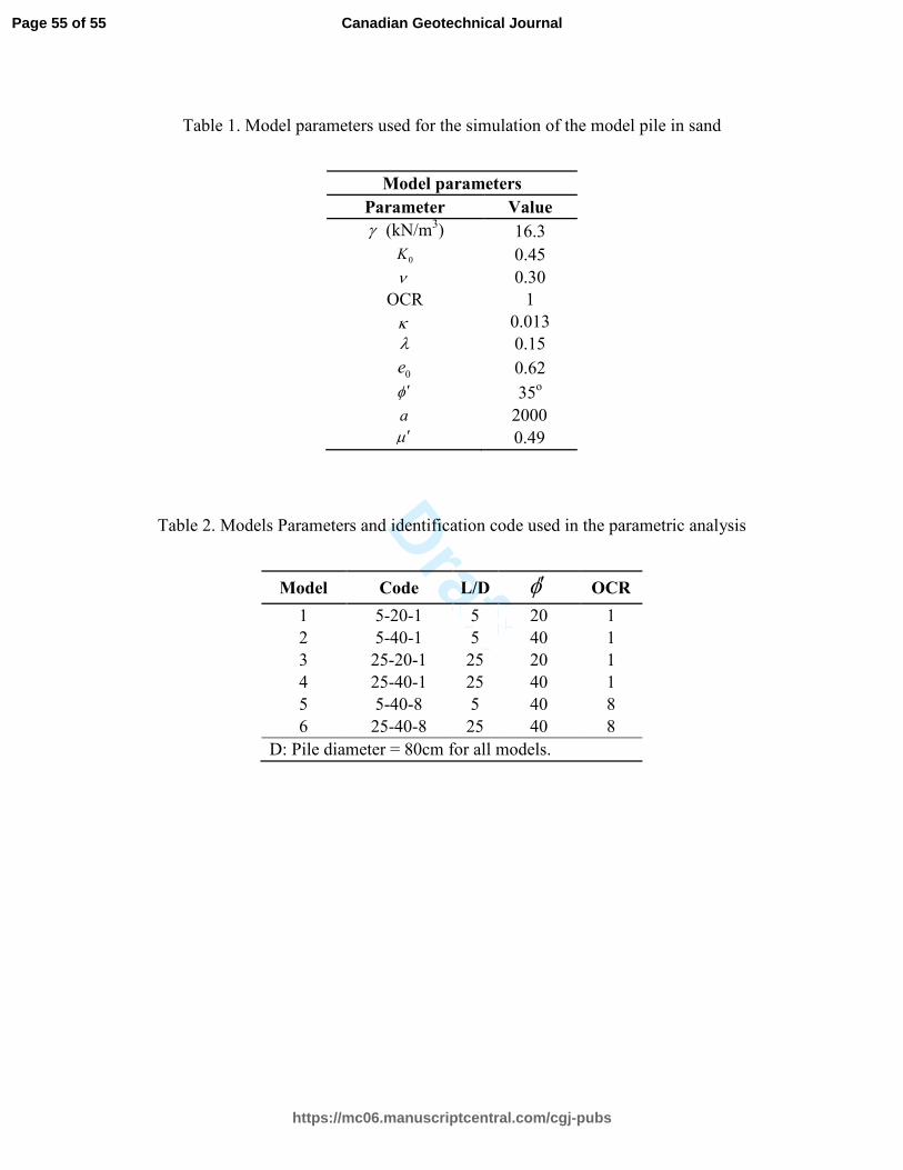
(2002) for stresses on the order of 100kPa (as in the initial state in the current analysis). Table 268

1 summarizes the mechanical parameters used in this simulation. 269

The mini-ICP2 test carried out by Jardine et al. (2013a) was simulated here in. In this test the 270

sand deposit was overloaded by a top membrane that had a central internal diameter of 271

200mm, just before the installation process. A base-pressurized membrane was also used, 272

with a surcharge pressure of 152kPa, which has generated an initial vertical stress along the 273

sand mass of approximately0 150V kPaσ = . A mini cone penetration test (CPT) was pushed in 274

the sample before the driving process, reproducing a quasi-constant tip cone resistance of 275

21 2C

q MPa= ± . A constant jacking rate of around 0.5mm/s was adopted during the semi static 276

(pushed-in) installation process. The pile diameter is D=36mm. 277

In the numerical simulations, the pile was considered to be a rigid material, greatly reducing 278

the computing time. Thus, the pile was introduced in the simulation as a moving boundary 279

condition. A constant vertical velocity of 20mm/s was applied to the pile until it was 280

completely installed. A Coulomb frictional contact type was used between the pile and the 281

surrounding soil with the interface friction coefficient obtained based on Tsuha et al. (2012) 282

results. Details of the contact algorithm used can be found in Bardenhagen et al. (2001) and 283

Lemiale et al. (2010). 284

The simulations took into consideration aforementioned sand properties for an OCR of 1. 285

Axisymmetric conditions were also considered, which have been recently presented for 286

GIMP by Nairn and Guilkey (2013). The background grid used the traditional uniform square 287

mesh with mesh cell of 0.25D, with 4 particles per cell. It was defined after a mesh-particle 288

discretization analysis resulting in a grid of 67x167 and a total of 44756 material points. The 289

boundary condition at the bottom side of the model was considered vertically fixed, and the 290

Page 13 of 55



Draft

14

lateral edge was horizontally fixed. An appropriate global damping factor (500/sec) was 291

added to the model since the beginning of the simulation, allowing to approach quasi-static 292

results without over damping. 293

The first loading stage was modeled using a distributed surface pressure of 150kPa. Only 294

after this initial case was the pile jacked process simulated. In the experimental setup, the 295

stresses inside the sand mass were measured with sensors located at different depths (z) at 296

certain radial distances from the pile’s axis (r). Figure 4 shows a schematic diagram of the 297

geometric variables that improves the understanding of the outcome results. The “x” in the 298

chart indicates experimental measurement points. 299

Figure 5 presents the radial displacement and the deformed shape obtained by the simulations 300

when using GIMP and the SubCam constitutive model. 301

Figure 6 shows the predicted radial stress at specific points inside the sand mass during the 302

installation process of the pile when simulated by using GIMP with either the MCC or the 303

SubCam models. The experimental values published by Jardine et al. (2013b) and Yang et al. 304

(2014) are also shown. The predicted radial stress values were normalized by 21cq MPa= , as 305

presented by Jardine et al. (2013a). In the vertical axis, values of h/R<0 represent stress 306

results for a specific sensor when the pile’s tip is above its particular depth level. In the case 307

of the sensor located at a depth of z=550mm, these authors only published measured results 308

for -5<h/R<5 (Figure 6c and 6d). 309

The results obtained using the MCC model differ from the experimental reference values, 310

albeit having similar trends. The maximum values of radial stress are experienced when the 311

pile tip is near the measuring sensor, decreasing once the pile passes by. The stresses for 312

r/R=3 (Figure 6a) are higher than those for r/R=8 (Figure 6b), exposing a tendency of 313

reduction of stresses as the horizontal distance to the pile axis increases. Simulations using 314

Page 14 of 55



Draft

15

the SubCam model tended to matched experiments better, although still with differences in 315

magnitude between experimental and numerical values. The simulated maximum radial 316

stresses were as much as 25 times higher than the initial stresses. For the four points studied 317

(Figure 4), the radial stresses were higher than the initial ones at the end of the installation 318

process. The radial stresses, at the end of the installation process, were as much as 3.5 times 319

higher than the initial radial stresses, as noticed for the point close to the pile (r/R=2). The 320

theoretical consideration of the densification process of the sand, as built in the SubCam 321

model, has indeed improved the match. The higher output of maximum stresses of this latter 322

model, when compared to output using the MCC, is associated to the increase in the rigidity 323

of the soil by the densification phenomenon that happens after pile penetration. Hence, for an 324

equal value of deformation the generated stresses in the SubCam model are generally higher. 325

The fact that the SubCam model uses the Matsuoka and Nakai failure criterion (Matsuoka 326

and Nakai 1985) also contributed to the slightly better results obtained with this model. When 327

the pile’s tip is penetrating into the soil, some extension stresses appear around it, which is 328

undoubtedly better reproduced with this particular criterion. 329

Figure 7 shows the vertical stress at specific points inside the sand mass during the pile 330

installation process. The measured values obtained by Jardine et al. (2013a) and the simulated 331

ones using GIMP with both MCC and SubCam models are presented. Similar to the radial 332

stress case, the vertical stress increased when the pile’s tip was near the depth level of the 333

measuring sensor. The maximum value is observed at h/R = -5. Once the pile passes by the 334

sensor the stress tends to decrease. However, contrary to what occurs in the radial case, the 335

final vertical stress at the end of installation is lower than the initial value for the data point 336

that is radially closer to the pile, thus indicating an upward movement of the soil around the 337

pile’s tip. 338

Page 15 of 55



Draft

16

For the vertical stresses, the SubCam model also gives better results than the MCC model, 339

especially near the peak value, when the pile’s tip is in the nearest position of the sensor 340

level. 341

Figure 8 presents the earth pressure coefficient (K) for the point located at z = 300mm and 342

r/R = 3 during the pile installation. At the beginning of the installation process, the value of K 343

is not affected at the depth of the sensor (z = 700mm) and is very close to 0 0.45K = . When 344

the pile’s tip is at / 5h R −� , the horizontal stress increases more than the vertical stress and 345

exceeds this last one, leading to a value of K >1. After the pile tip passes the depth level of 346

the measuring sensor the value of K rapidly decreases, still reaching values greater than 1 at 347

the end of the installation process. This outcome characterizes a pattern of earth pressures 348

that resembles the development of passive pressures around the pile’s shaft. Again, the 349

SubCam model led to results that are closer to the experimental values. 350

Figure 9 shows the stress path during the pile installation process for a point at z = 700mm 351

and r/R = 3, obtained using the MCC and the SubCam models. This path resembles those 352

from oedometric loading tests, at least until the pile’s tip has reached the level of the 353

measuring sensor level (h/R = 1.7 for the MCC and h/R = -1.1 for the SubCam). After this 354

stage is reached, a rapid unloading path follows. Sheng et al. (2005) also showed similar 355

behavior in their numerical analyses with a critical state model, where a sharp decrease in 356

stress is observed soon after a peak value is reached. They observed that such a phenomenon 357

is associated with the formation of a plastic softening zone around the pile. 358

Figure 10 shows the radial stresses in two horizontal sections at different depths after the pile 359

installation process is completed. The maximum values for each section are near r/R=3. The 360

far the points are from the pile axis the smaller the stresses are. Besides, the stresses increase 361

with depth until the pile’s tip region. Near the shaft (r/R=1-3) the radial stresses show a 362

Page 16 of 55



Draft

17

decrease when compared with the trend. Such reduction near the shaft was linked by Yang et 363

al. (2010) with a) with some particular factors, as (a) strain path reversals that occur as the 364

soil flows through the shoulder of the pile’s tip. This reduces the stresses and leads to arching 365

with rθσ σ′ ′> near the shaft, (b) the development of an annulus of intensely compressed and 366

sheared sand around the shaft. The simulations captured relatively well the reduction of 367

stresses around the shaft, sustaining the first hypothesis advocated by Yang et al. (2010). 368

Lower values of radial stresses were also obtained when they were compared to the measured 369

ones. Also, a faster reduction of the magnitude of the stresses can be observed. For points that 370

are far from the pile’s axis (r/R=13), the stresses are almost equal the initial values. 371

Figure 11 shows the displacement path obtained using GIMP and the SubCam model during 372

the installation process. Most of the displacements occur when the pile’s tip has a relative 373

depth between h/R=-10 and 10. For the point closer to the pile’s axis (r/R=3), after the pile’s 374

tip pass through the point level (h/R=~0-1.1) the vertical displacement changes in direction 375

and the point goes up. This explains the decrease that appears in the vertical stress once the 376

pile’s tip passes through the sensor level (Figure 7a). The upwards movement is actually a 377

consequence of the flow of soil around the shoulder of the pile’s tip (White and Bolton 2004). 378

For the point farther from the pile’s axis (r/R=8), this features doesn’t appear, so the vertical 379

displacement is always downwards. For both points, the horizontal displacement increases 380

until the pile’s tip pass through the point level (h/R=~0-1.1), after that, a little decrease 381

occurs. This movement contributes to the decrease in the radial stress when the pile’s tip pass 382

the point level (Figure 6). 383

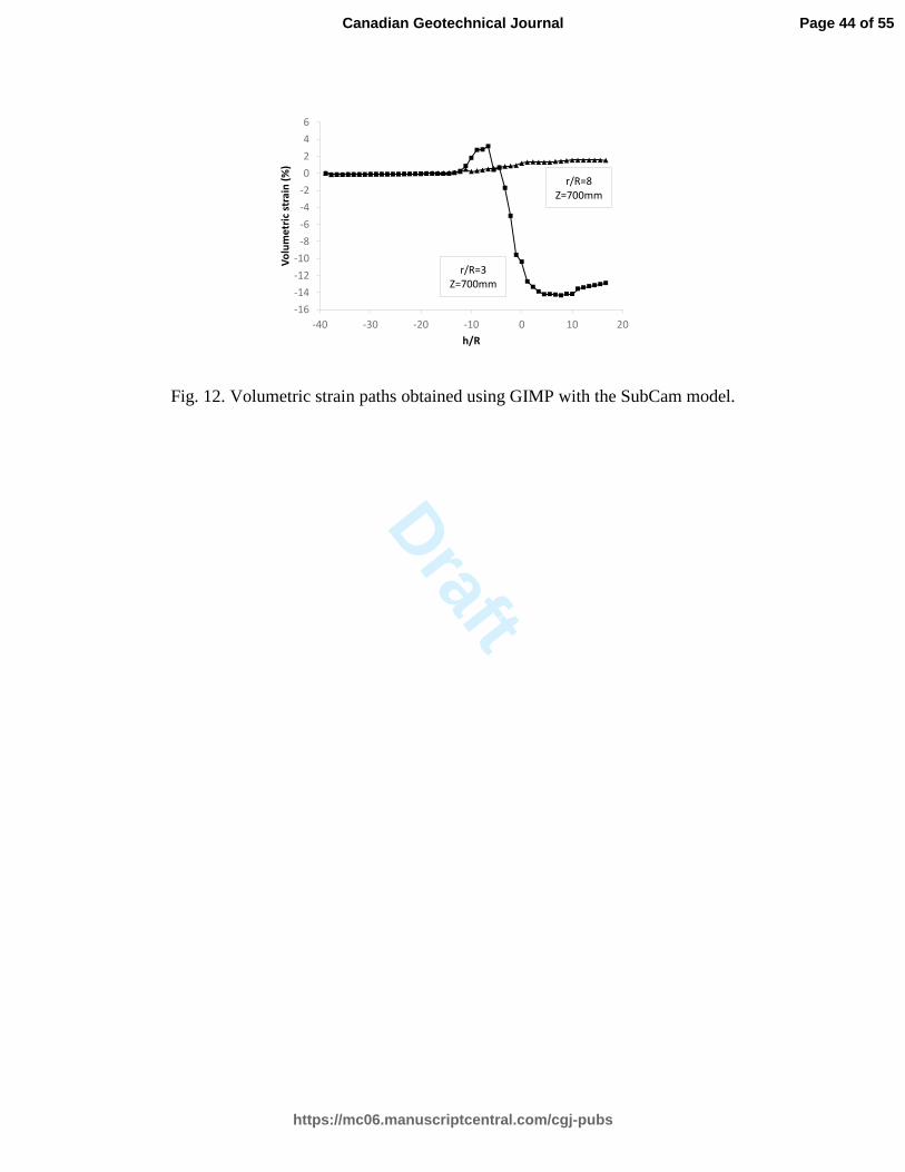
Volumetric strain paths obtained during the installation process are shown in Figure 12. For 384

the point nearest to the pile’s axis (r/R=3), compression is observed when the pile tip gets 385

closer to the point level (-10<h/R<-6), this is followed by a strong dilation when the pile tip is 386

Page 17 of 55



Draft

18

within a distance of 6 radii. Ones the pile’s tip pass the point level, a small compression is 387

observed until h/R=10. A net increase in volume is then obtained for this point (12%). This 388

behavior is similar to the results presented by White and Bolton (2004) for points nearest to 389

the pile’s axis (r/R<2), inside the zone defined as very near field behavior zone. 390

For the point far from the pile’s axis (r/R=8), a monotonically increase of compression occurs 391

during the pile installation process. This trend is in good agreement with the experimental 392

results of White and Bolton (2004) for points located inside the zone defined by the authors 393

as far field behavior zone. 394

The end points of the volumetric strain paths indicate the variation in density after the 395

installation process. The strong dilation in the near field creates a zone of soil close to the pile 396

shaft that is less dense than the more distant soil. 397

The simulated results can be considered in good agreement with the experimental ones for 398

applications in foundation engineering. However, improvement can be done to the model to 399

perfectly match with the experimental outputs. Some important constitutive characteristic can 400

be added such as, anisotropy, grain breakage, strain dependency and friction angle stress 401

dependency. 402

Parametric analysis and effect of friction fatigue 403

A parametric analysis was performed to evaluate the influence of the installation process on 404

the bearing capacity of a typical pushed-in pile in granular soil. The SubCam constitutive 405

model was used for the soil, and the pile was considered infinitely rigid. The analysis was 406

performed using axisymmetric conditions starting with a 0K geostatic stress field. The 407

installation process was simulated by applying a constant vertical velocity (20mm/s) to the 408

Page 18 of 55



Draft

19

pile until it was completely driven. This feature reflects better the (pushed-in) installation of a 409

jacked pile. 410

The differences between the behavior of a jacked pile and a driven pile have been presented 411

by Yang et al. (2006) and Zhang and Wang (2009). They concluded that the shaft resistance 412

of jacked piles is generally stiffer and stronger than that of driven ones. 413

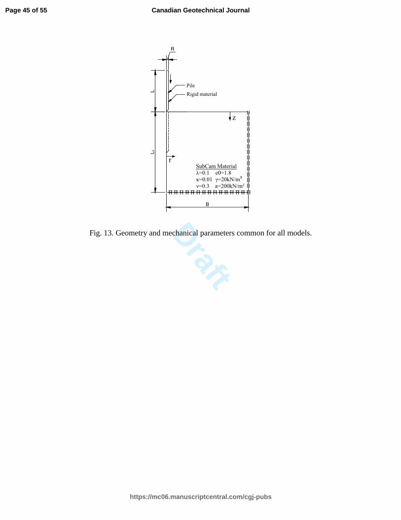
Figure 13 shows both geometry and mechanical parameters common for all simulated cases. 414

Table 2 presents the material and the normalized geometric variables considered for all 415

analyses. In this table, the numerical cases are coded by an identification number (L/D-φ ′ -416

OCR), followed by the slenderness of the pile, the friction angle and the overconsolidation 417

ratio of the soil. The mesh and number of particles per cell used in these simulations was the 418

same of the previous presented case (mesh cell dimension = 0.25D and 4 particles per cell). 419

The boundary condition at the bottom side of the model was considered vertically fixed, and 420

the lateral edge as horizontally fixed. 421

Figures 14 to 16 show the radial stress at the shaft of the pile after its installation. As one can 422

see, the variation of stress along depth is almost linear until the tip of the pile (0.7L for the 423

shortest piles and 0.9L for longest ones). At this particular region there is a sudden increase in 424

stress followed by a sharp decrease. This behavior resembles the idealized pattern shown in 425

Figure 1, which encourages the authors to affirm that the analyses tended to approach the 426

“real” experimental phenomena. The increase of the radial stress ratio near the pile’s tip 427

occurs because this zone experiences less shear cycle than other depths during the installation 428

process. One can also notice that the radial stress increment in relation to the initial stress 429

( )rf riσ σ is higher for the models with 40φ ′ = o

than those with 20φ ′ = o . For the former 430

ones, the weighted mean increment stress along depth is around 5, whereas for the latter ones 431

it drops to values in the range of 1.5. 432

Page 19 of 55



Draft

20

Figure 17 depicts the large influence of the friction angle on the value of the radial stress after 433

installation of the pile. This phenomenon can be explained by observing the stress path 434

followed by a point near the pile’s shaft during penetration. The plastic strains are much 435

higher than the elastic ones, hence the direction of the deformations are controlled by the 436

plastic strains. For the constitutive model used herein, the plastic volumetric strains are 437

higher for the soil with higher φ′ values (Figure 18). The higher strength granular materials, 438

idealized herein, tend to have higher values of normal stress, consequently, for this case, 439

higher values of radial stress. 440

Figure 19 shows the influence of the length of the pile, on the radial stresses at the end of the 441

installation process. The relative increment in the radial stress to increases in the friction 442

angle tends to be higher for the shortest pile (L/D=5) than for the longest one (L/D=25). Also, 443

the longer is the pile, the lower will be the radial stress at equivalent depth. By noticing that, 444

at a particular depth, the value of h/R is larger for the pile with L/D=25, one concludes that a 445

“friction fatigue phenomenon” (or h/R effect) is probably the cause of such a result. 446

Experimental evidence tends to back up this observation, which can be attributed to the 447

gradual densification of the soil adjacent to the pile’s shaft under the cyclic shearing action of 448

installation (White and Bolton 2004). As commented before, Sheng et al. (2005) also 449

associated this phenomenon with the softening of the soil one radius around the pile, because 450

of a plastic expansion of the material in this particular zone. 451

The effect of the overconsolidation ratio (OCR) in the final radial stress mobilized at the 452

pile’s shaft is negligible, as clearly shown in Figure 20. The authors did not find any 453

experimental data that confirms this phenomenon, but neither the equation proposed by 454

Randolph et al. (1994) (Eq. 1) nor the one by Jardine et al. (2005) consider the OCR effect. 455

Sheng et al. (2005) evidenced that the general pattern of the stress path followed by a soil 456

Page 20 of 55



Draft

21

point near the pile is not significantly influenced by the OCR during pile installation. A 457

possible explanation is given by the fact that the stress path inside the yield surface is very 458

small compared to the one on the yield surface itself. Hence, one can expect the stress 459

response of the soil to be similarly close at distinct conditions of overconsolidation ratio. 460

Figure 21 shows the profile of the earth pressure coefficient along depth for piles with 461

distinct lengths (or slenderness ratios L/D). The presented coefficient ( )rf ViK σ σ′ ′=

is 462

actually a ratio between the horizontal effective stress at the end of the installation process 463

and the constant vertical effective geostatic stress. A similar pattern to the radial stress profile 464

is also noticed for this coefficient, which is logical. Also, for the soils with a higher granular 465

strength ( )φ′ , a higher K is obtained, because as mentioned before the horizontal stress is 466

strongly influenced by the friction angle of the soil. 467

Effect of installation process on ultimate shaft resistance 468

One of the most important variables that can be derived from the radial stress around the 469

pile’s shaft is the ultimate shaft resistance ( )sQ of the pile – or lateral bearing capacity. 470

Considering that sQ is related to the ultimate shaft friction ( )sτ , and this last one correlates to 471

both the horizontal effective stress ( )hσ′ acting on the shaft and the effective (remoulded) 472

angle of friction between soil and pile (δ ′ ), one can write: 473

0 0

tan

L L

s s s s rQ A dz A dzτ σ δ′ ′= =∫ ∫ (12) 474

With equation (12) one notices that by considering that δ ′ does not change throughout the 475

installation of the pile, the relation between ultimate shaft resistance considering the 476

installation effects ( )f

sQ and not considering ( )0

sQ only depends on the horizontal effective 477

Page 21 of 55



Draft

22

stress at the pile’s shaft immediately before failure (lateral shearing). Therefore, new 478

simulations were done similar to those previously shown, by applying a further prescribed 479

displacement of D/30 on the pile once its installation was finalized. This added displacement 480

effect tended to simulate a lateral friction failure. 481

482

Figure 22 shows the relation 0f

s sQ Q for the simulated cases. As one can see, the increase in 483

shaft resistance is higher for short piles (models 1, 2 and 5) than for long ones. This 484

difference is caused by aforementioned friction fatigue effect on longer piles. The increase is 485

also higher for the piles immersed in a high strength soil (models 2, 4, 5 and 6). As the 486

previous case, the OCR effect is negligible. 487

By defining the relationship between the ultimate shaft resistance of a pushed-in and of an 488

excavated pile as pushed excavated

s sQ Q , one can also reach interesting conclusions. This ratio can be 489

empirically defined by Brazilian (SPT pile design) methods that somehow take into account 490

the installation process (from experimental load tests on long piles), as for instance the 491

methods of Aoki and Velloso (1975) and Décourt and Quaresma (1978). These latter 492

empirical approaches indicate, for piles installed in the same soil profile, ratios 493

1.18drivenpile excavated

s sQ Q = for clay and 2 for sand (long or high L/D piles). So, considering in a 494

simplified manner that 0 excavated

s sQ Q≈ , the relation 0f

s sQ Q can be directly compared to the ratio 495

pushed excavated

s sQ Q . With such an exercise one derives empirical values of drivenpile excavated

s sQ Q that 496

are in the same order than those numerically predicted by both models 3 and 4, which again is 497

an encouraging (experimental vs. numerical) outcome. 498

Conclusions 499

The installation process of single jacked (push-in) piles in granular soils can be modelled 500

with the generalized interpolation material point method, or GIMP, by adopting a Coulomb 501

Page 22 of 55



Draft

23

friction model at the contact soil/pile. The adopted numerical method was able to handle this 502

large deformation problem in a robust and practical way. 503

Two constitutive models have been implemented and tested. The final response of the driven 504

pile with the modified cam clay model (MCC) did unfortunately not agree well with the small 505

scale experimental results. Because only a few adjustments were necessary to turn the MCC 506

into the subloading cam clay model (SubCam), the latter was also implemented and tested 507

herein. The SubCam model clearly provides a better match between numerical and 508

experimental outputs, being therefore advantageous to use it in the simulation of problems of 509

this kind. Indeed, the SubCam model does consider in a better and proper way the granular 510

soil densification after pile insertion, and can differentiate the response from triaxial or 511

compression loading paths. 512

Furthermore, for typical geometries adopted in jacked piles in granular soils, the post 513

installation lateral stress coefficient K reaches values as high as 2 times the original earth 514

pressure coefficient K0. From the spatial distribution of stresses after pile installation, it 515

seems that horizontal stresses in the soil can be very high when compared to the initial 516

geostatic horizontal values (K0 times the vertical effective stress). For instance, at a radial 517

distance around 4 times the pile diameter from the pile´s axis (r/D=4), horizontal mobilized 518

stresses can be as much as 2 times higher than the original effective values. The analyses 519

have also attested some observations in literature that the overconsolidation ratio (OCR) does 520

not significantly affect the output response of the pile’s installation process. 521

The simulations were able to capture the effect of friction fatigue in long slender piles 522

installed in sands. The results suggest that the friction fatigue effect shows the effect of stress 523

history in the soil element resulting in evolving strength/stiffness properties. 524

Page 23 of 55



Draft

24

A final and broad conclusion of the study can be derived from the importance demonstrated 525

by the analyses to effectively consider the penetration process of driven (push-in type) piles 526

in sands. The installation phenomena clearly changes some post execution geotechnical 527

variables of the granular material, enhancing for instance the bearing capacity of the pile, 528

densifying the surrounding media, or increasing the stress levels all around the foundation – 529

generally in a simultaneous manner. It is then concluded that to properly understand the post 530

installation behavior of driven piles in sands, one must account for the installation effect 531

itself, either by numerical or by analytical simplified approaches. 532

Acknowledgements 533

The authors acknowledge and thank the Brazilian Government through its research 534

sponsorship organizations CAPES and CNPq that allowed the first author to carry on and 535

finalize his D.Sc. Thesis in the Geotechnical Post Graduation Program of the University of 536

Brasília. The support from colleagues from the Research Group on Foundations and In Situ 537

Testing (GPFees, www.geotecnia.unb.br/gpfees) was also essential to the successful outcome 538

of this project. 539

Page 24 of 55



Draft

25

References

Aoki, N., and Velloso, D. A. 1975. An Aproximate Method to Estimate the Bearing Capacity

of Piles. In Congreso Panamericano de Mecánica de Suelos y Cimentaciones PASSMFE

(pp. 367–376). Buenos Aires.

Bardenhagen, S. G., Brackbill, J. U., and Sulsky, D. 2000. The material-point method for

granular materials. Computer Methods in Applied Mechanics and Engineering, 187(3–

4), 529–541. http://doi.org/10.1016/S0045-7825(99)00338-2

Bardenhagen, S. G., Guilkey, J. E., Roessig, K. M., Brackbill, J. U., and Witzel, W. M. 2001.

An Improved Contact Algorithm for the Material Point Method and Application to

Stress Propagation in Granular Material. Computer Modeling in Engineering and

Sciences, 2(4), 509–522.

Bardenhagen, S. G., and Kober, E. M. 2004. The Generalized Interpolation Material Point

Method. Tech Science Press, 5(6), 477–495.

Beuth, L., Benz, T., and Vermeer, P. A. 2007. Large deformation analysis using a quasi-static

Material Point Method. In Computer Methods in Mechanics (pp. 1–6). Lodz-Spala.

Décourt, L., and Quaresma, A. R. 1978. Capacidade de carga de estacas a partir de valores de

SPT. In Congresso Brasileiro de Mecânica de Solos e Fundações (pp. 215–224). São

Paulo.

De Gennaro, V. and Frank, R. 2002. Insight into the simulation of calibration chamber tests.

In Proc. 5th Eur. Conf. Numer. Methods Geotech. Engng (pp. 169-177). Paris.

Dijkstra, J., Broere, W., and Heeres, O. M. 2011. Numerical simulation of pile installation.

Computers and Geotechnics, 38(5), 612–622.

http://doi.org/10.1016/j.compgeo.2011.04.004

Page 25 of 55



Draft

26

Doherty, P., and Gavin, K. 2011. The Shaft Capacity of Displacement Piles in Clay: A State

of the Art Review. Geotechnical and Geological Engineering, 29(4), 389–410.

Retrieved from http://www.springerlink.com/index/10.1007/s10706-010-9389-2

Farias, M. M., Nakai, T., Shahin, H. M., Pedroso, D. M., Passos, P. G. O., and Hinokio, M.

2005. Ground Densification due to sand compaction piles. Soils and Foundations, 45(2),

167–180.

Farias, M. M., Pedroso, D. M., and Nakai, T. 2009. Automatic substepping integration of the

subloading tij model with stress path dependent hardening. Computers and Geotechnics,

36(4), 537–548. http://doi.org/10.1016/j.compgeo.2008.11.003

Fleming, K., Weltman, A., and Randolph, M. F. 2009. Piling Engineering. (T. Francis, Ed.)

(Third Edit). London.

Gue, S. S. 1984. Ground Heave Around Driven Piles in Clay (PhD. Thesis). University of

Oxford.

Hamad, F. 2016. Formulation of the axisymmetric CPDI with application to pile driving in

sand. Computers and Geotechnics, 74, 141–150.

http://doi.org/10.1016/j.compgeo.2016.01.003

Hashiguchi, K., and Ueno, M. 1977. Elastoplastic Constitutive Laws of Soils. In 9th ICSMFE

Special Session 9 (pp. 73–82). Tokyo.

Hira, M., Hashiguchi, K., Ueno, M., and Okayasu, T. 2006. Deformation behavior of shirasu

soil by yhe extended subloading surface model. Lowland Technology International,

8(1), 37–46.

Jardine, R. J., Chow, F., Overy, R., and Standing, J. 2005. ICP Design Methods for Driven

Piles in Sands and Clays. London: Thomas Telford Publishing.

Page 26 of 55



Draft

27

Jardine, R. J., Zhu, B. T., Foray, P. Y., and Yang, Z. X. 2013a. Measurement of stresses

around closed-ended displacement piles in sand. Géotechnique, 63(8), 1–17.

Jardine, R. J., Zhu, B. T., Foray, P., and Yang, Z. X. 2013b. Interpretation of stress

measurements made around closed-ended displacement piles in sand. Géotechnique,

63(8), 613–627. Retrieved from http://dx.doi.org/10.1680/geot.9.P.138

Lemiale, V., Nairn, J. A., and Hurmane, A. 2010. Material Point Method Simulation of Equal

Channel Angular Pressing Involving Large Plastic Strain and Contact Through Sharp

Corners. Computer Modeling in Engineering and Science, 70(1), 41–66.

Matsuoka, H., and Nakai, T. 1985. Relationship among Tresca, Mises, Mohr-Coulomb and

Matsuoka-Nakai failure criteria. Soils and Foundations, 25(4), 123–128.

Nairn, J. A. 2011. Source code and documentation for NairnMPM Code for Material Point

Calculations. http://oregonstate. edu/~nairnj/.

Nairn, J. A., and Guilkey, J. E. 2013. Axisymmetric form of the generalized interpolation

material point method. International Journal for Numerical Methods in Engineering, 0,

1–24. http://doi.org/10.1002/nme

Nakai, T. 2013. Constitutive Modeling of Geomaterials (Taylor & F). Boca Raton: CRC

Press.

Nakai, T., and Hinokio, M. 2004. A simple elastoplastic model for normally and over

consolidated soils with unified material parameters. Soils and Foundations, 44(2), 53–

70.

Nguyen, G. D., Yang, Z. X., Jardine, R. J., Zhang, C., and Einav, I. 2014. Theoretical

breakage mechanics and experimental assessment of stresses surrounding piles

penetrating into dense silica sand. Géotechnique Letters, 4(January-March), 11–16.

Page 27 of 55



Draft

28

http://doi.org/10.1680/geolett.13.00075

Pedroso, D. M. 2006. Representação Matemática do Comportamento Mecânico Cíclico de

Solos Saturados e Não Saturados (Teses de Doutorado, Departamento de Engenharia

Civil e Ambiental). Universidade de Brasília.

Pedroso, D. M., Farias, M. M., and Nakai, T. 2005. An interpretation of subloading tij model

in the context of conventional elastoplasticity theory. Soils and Foundations, 45(4), 61–

77.

Phuong, N. T. V., van Tol, A. F., Elkadi, A. S. K., and Rohe, A. 2014. Modelling of pile

installation using the material point method (MPM). In M. Hicks, R. B. J. Brinkgreve, &

A. Rohe (Eds.), Numerical Methods in Geotechnical Engineering (pp. 271–276). Delft:

Taylor & Francis.

Phuong, N. T. V., van Tol, A. F., Elkadi, A. S. K., and Rohe, A. 2016. Numerical

investigation of pile installation effects in sand using material point method. Computers

and Geotechnics, 73, 58–71. http://doi.org/10.1016/j.compgeo.2015.11.012

Randolph, M. F. 2003. Science and empiricism in pile foundation design. Géotechnique,

53(10), 847–875. http://doi.org/10.1680/geot.2003.53.10.847

Randolph, M. F., Carter, J. P., and Wroth, C. P. 1979. Driven piles in clay-the effects of

installation and subsequent effects consolidation. Géotechnique, 29(4), 361–393.

Randolph, M. F., Dolwin, J., and Beck, R. 1994. Design of driven piles in sand.

Géotechnique, 44(3), 427–448.

Sadeghirad, A., Brannon, R. M., and Burghardt, J. 2011. A convected particle domain

interpolation technique to extend applicability of the material point method for problems

involving massive deformations. International Journal for Numerical Methods in

Page 28 of 55



Draft

29

Engineering, 86(12), 1435–1456. http://doi.org/10.1002/nme

Sheng, D., Eigenbrod, K. D., and Wriggers, P. 2005. Finite element analysis of pile

installation using large-slip frictional contact. Computers and Geotechnics, 32(1), 17–

26. http://doi.org/10.1016/j.compgeo.2004.10.004

Sheng, D., Nazem, M., and Carter, J. P. 2009. Some computational aspects for solving deep

penetration problems in geomechanics. Computational Mechanics, 44(4), 549–561.

http://doi.org/10.1007/s00466-009-0391-6

Slatter, J. W. 2000. The Fundamental Behaviour of Displacement Screw Piling Augers.

Monash University.

Solowski, W. T., and Sloan, S. W. 2015. Evaluation of material point method for use in

geotechnics. International Journal for Numerical and Analytical Methods in

Geomechanics, 39, 685–701. http://doi.org/10.1002/nag.2321

Sulsky, D., Chen, Z., and Schreyerb, H. L. 1994. A Particle Method for History-Dependent

Materials. Computer Methods in Applied Mechanics and Engineering, 118(1), 179–196.

Tsuha, C. H. C., Foray, P. Y., Jardine, R. J., Yang, Z. X., Silva, M., and Rimoy, S. 2012.

Behaviour of displacement piles in sand under cyclic axial loading. Soils and

Foundations, 52(3), 393–410. http://doi.org/10.1016/j.sandf.2012.05.002

White, D. J., and Bolton, M. D. 2004. Displacement and strain paths during plane-strain

model pile installation in sand. Géotechnique, 54(6), 375–397.

White, D. J., and Lehane, B. M. 2004. Friction fatigue on displacement piles in sand.

Géotechnique, 54(10), 645–658. http://doi.org/10.1680/geot.2004.54.10.645

Wieckowski, Z. 2004, October. The material point method in large strain engineering

problems. Computer Methods in Applied Mechanics and Engineering.

Page 29 of 55



Draft

30

http://doi.org/10.1016/j.cma.2004.01.035

Yang, J., Tham, L. G., Lee, P. K. K., Chan, S. T., and Yu, F. 2006. Behaviour of jacked and

driven piles in sandy soil. Géotechnique, 56(4), 245–259.

http://doi.org/10.1680/geot.2007.57.5.475

Yang, Z. X., Jardine, R. J., Zhu, B. T., and Rimoy, S. P. 2014. Stresses Developed around

Displacement Piles Penetration in Sand. Journal of Geotechnical and Geoenvironmental

Engineering, 140(3), 1–13. http://doi.org/10.1061/(ASCE)GT.1943-5606.0001022.

Zabala, F. 2010. Modelación de problemas geotécnicos hidromecánicos utilizando el método

del punto material. Universidad Politécnica de Catalunya.

Zdravkovic, L., and Carter, J. P. 2008. Contributions to Géotechnique 1948–2008:

Constitutive and numerical modelling. Géotechnique, 58(5), 405–412.

Zhang, C., Yang, Z. X., Nguyen, G. D., Jardine, R. J., and Einav, I. 2014. Theoretical

breakage mechanics and experimental assessment of stresses surrounding piles

penetrating into dense silica sand. Géotechnique Letters, 4(January-March), 11–16.

http://doi.org/10.1680/geolett.13.00075

Zhang, L. M., and Wang, H. 2009. Field study of construction effects in jacked and driven

steel H-piles. Géotechnique, 59(1), 63–69. http://doi.org/10.1680/geot.2008.T.029

Zhang, Z., and Wang, Y. 2014. Examining Setup Mechanisms of Driven Piles in Sand Using

Laboratory Model Pile Tests. Journal of Geotechnical and Geoenvironmental

Engineering, 141(3), 1–12. http://doi.org/10.1061/(ASCE)GT.1943-5606.0001252.

Page 30 of 55



Draft

31

Figure caption list

Fig. 1. Idealized and field profiles of shaft friction with depth (modified from Randolph et al.

1994)

Fig. 2. Subloading surface and definition of variable ρ (after Nakai 2013)

Fig. 3. Schematic diagram of pile installation test showing one example instrument layout

(Jardine et al. 2013a)

Fig. 4. Schematic diagram of the geometric reference for the results and sensors position.

Fig. 5. Horizontal displacement shade and deformed shape for the soil with the pile driven at

distinct depth levels.

Fig. 6. Radial stress during the pile installation process measured (Jardine et al. 2013a; Yang

et al. 2014) and simulated using GIMP and MCC and SubCam models

Fig. 7. Vertical stress during the pile installation process measured (Jardine et al. 2013a) and

simulated using GIMP and MCC and SubCam models

Fig. 8. Earth pressure coefficient for a specific point (z=700m and r/R=3) during the

installation process.

Fig. 9. Stress path during the pile installation process for a specific point (z=700mm and

r/R=3)

Fig. 10. Radial stresses in horizontal sections after the pile installation process, measured

(Jardine et al. 2013b) and simulated using GIMP and MCC and SubCam models.

Fig. 11. Simulated displacement path during the pile installation process using GIMP with the

SubCam model.

Page 31 of 55



Draft

32

Fig. 12. Volumetric strain paths obtained using GIMP with the SubCam model.

Fig. 13. Geometry and mechanical parameters common for all models.

Fig. 14. Radial stresses at the pile´s shaft after the installation process. Model 1 (5-20-1).



Fig. 17. Influence of the φ ′ value on the normalized radial stress at the pile´s shaft after the


Fig. 18. Schematic diagram of stress path and plastic strains for a point near the pile´s shaft

during the pile penetration.

Fig. 19. Influence of the length in the normalized radial stress at the pile´s shaft after the


Fig. 20. Influence of the OCR on the normalized radial stress at the pile´s shaft after the


Fig. 21. Earth pressure coefficient ( )rf Viσ σ′ ′ after the installation process.

Fig. 22. Relation between the ultimate shaft resistance considering and not considering the

installation effect ( )0f

s sQ Q .

Page 32 of 55



Draft

Fig. 1. Idealized and field profiles of shaft friction with depth (modified from Randolph et al. 1994)

Page 33 of 55



Draft

Fig. 2. Subloading surface and definition of variable (after Nakai, 2013)

Page 34 of 55



Draft

Fig. 3. Schematic diagram of pile installation test showing one example instrument layout

(Jardine et al., 2013a)

Page 35 of 55



Draft

Fig. 4. Schematic diagram of the geometric reference for the results and sensors position.

Page 36 of 55



Draft

a) 0mm b) 200mm

c) 600mm d) 1000mm

e) Zoom in for 600mm f) Zoom in for 1000mm

-13 18 (mm)

Fig. 5. Horizontal displacement shade and deformed shape for the soil with the pile driven at

distinct depth levels.

Page 37 of 55



Drafta) b)

c) d)

Fig. 6. Radial stress during the pile installation process measured (Jardine et al. 2013(a);Yang et

al. 2014) and simulated using GIMP and MCC and SubCam models

Page 38 of 55



Drafta) b)

Fig. 7. Vertical stress during the pile installation process measured (Jardine et al. 2013(a) and

simulated using GIMP and MCC and SubCam models

Page 39 of 55



Draft

Fig. 8. Earth pressure coefficient for a specific point (z=700m and r/R=3) during the installation

process.

Page 40 of 55



Draft

a) MCC b) SubCam

Fig. 9. Stress path during the pile installation process for a specific point (z=700mm and r/R=3)

Page 41 of 55



DraftFig. 10. Radial stresses in horizontal sections after the pile installation process, measured

(Jardine et al. 2013(a) and simulated using GIMP and MCC and SubCam models.

Page 42 of 55



Draft

Fig. 11. Displacement path obtained during the pile installation process using GIMP with

the SubCam model.

Page 43 of 55



Draft

Fig. 12. Volumetric strain paths obtained using GIMP with the SubCam model.

Page 44 of 55



Draft

Fig. 13. Geometry and mechanical parameters common for all models.

Page 45 of 55



Draft

a) b)

Fig. 14. Radial stresses at the pile’s shaft after the installation process. Model 1 (5-20-1).

Page 46 of 55



Draft

a) b)

Fig. 15. Radial stresses at the pile’s shaft after the installation process. Model 2 (5-40-1).

Page 47 of 55



Draft

a) b)


Page 48 of 55



Draft

a) b)

Fig. 17. Influence of the value on the normalized radial stress at the pile´s shaft after the


Page 49 of 55



Draft

Fig. 18. Schematic diagram of stress path and plastic strains for a point near the pile´s shaft

during the pile penetration.

Page 50 of 55



Draft

a) b)

Fig. 19. Influence of the length in the normalized radial stress at the pile´s shaft after the


Page 51 of 55



Draft

a) b)

Fig. 20. Influence of the OCR on the normalized radial stress at the pile´s shaft after the


Page 52 of 55



Draft

a) 20o b) 40o

Fig. 21. Earth pressure coefficient rf Vi after the installation process.

Page 53 of 55



Draft

Fig. 22. Relation between the ultimate shaft resistance considering and not considering the

installation effect 0f

s sQ Q .

Page 54 of 55



Draft

Table 1. Model parameters used for the simulation of the model pile in sand

Model parameters

Parameter Value

γ (kN/m3) 16.3

0K 0.45

ν 0.30

OCR 1

κ 0.013

λ 0.15

0e 0.62

φ ′ 35o

a 2000

µ ′ 0.49

Table 2. Models Parameters and identification code used in the parametric analysis

Model Code L/D

OCR

1 5-20-1 5 20 1

2 5-40-1 5 40 1

3 25-20-1 25 20 1

4 25-40-1 25 40 1

5 5-40-8 5 40 8

6 25-40-8 25 40 8

D: Pile diameter = 80cm for all models.

φ′

Page 55 of 55



Documents

pile, installation process, numerical modelling, material ... · 88 elements geotechnical codes which incorporates Lagrangian formulations are unsuitable to 89 simulate these types