Embed Size (px)
Citation preview
E D W A R D B R O W N
I N T R O D U C T O R Y T O P I C S I N A S T R O N O M Y
P L A N E T S A N DT E L E S C O P E S
O P E N A S T R O P H Y S I C S B O O K S H E L F
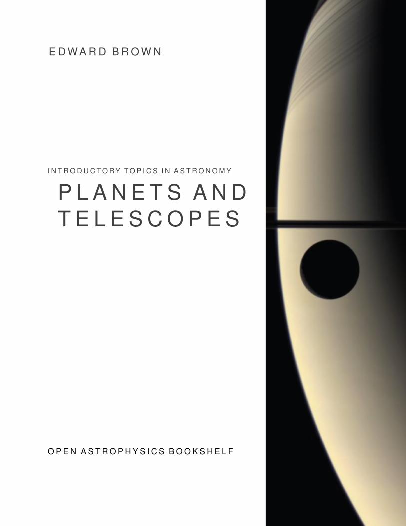
About the cover: an image of Rhea occulting Saturn, as captured by the Cassini spacecraft.Credit: Cassini Imaging Team, SSI, JPL, ESA, NASA
© 2017 Edward Browngit version 125f41c3 . . .
cbna
Except where explicitly noted, this work is licensed under the Creative Commons Attribution-NonCommercial-ShareAlike 4.0 International (CC BY-NC-SA 4.0) license.
Preface
These notes were written while teaching (and revamping) a one-semester introductory astronomy course, “Planets and Telescopes”at Michigan State University during 2015, 2016, and 2017. The back-ground required was introductory calculus and first-year physics.The reason for the odd juxtaposition of topics—planets and telescopes—is that the course was created from the merger of two undergraduatecourses, one of which was a laboratory course. During 2015 and 2016,Prof. Laura Chomiuk and I co-taught the course, with Laura han-dling the laboratory component and I the lecture. In 2017 the coursebecame fully merged under one instructor with a graduate teachingassistant and undergraduate learning assistants helping to run thelaboratory portion. These notes comprise the lecture materials for thecourse.
As described in the white paper detailing the course revisions1, 1 Edward F. Brown, Laura Chomiuk,Laura Shishkovsky, and AndrewBundas. Development of a sophomorelevel astronomy course on planetsand telescopes. White paper detailingrevisions to AST 208, MSU, 2015. URLhttps://www.authorea.com/19544/
7GTRKXg6i69rNPihL7S99g
the astronomy group at MSU set out learning outcomes for the un-dergraduate astronomy program that included an increased empha-sis on analysis and interpretation of data. In response to these goals,the revised course “Planets and Telescopes” uses “real” data and ob-servatory archives; introduces rudimentary data analysis in both thelecture and lab components; and encourages collaborative work via aflipped classroom model.
In the first iteration of the course we used Lissauer and de Pater2 2 Jack J. Lissauer and Imke de Pater.Fundamental Planetary Science: Physics,Chemistry and Habitability. CambridgeUniversity Press, 2013
and Bennett et al.3 as primary texts. We found, however, that we
3 Jeffrey O. Bennett, Megan O. Donahue,Nicholas Schneider, and Mark Voit. TheCosmic Perspective. Addison-Wesley, 7thedition, 2013
needed to spend more time on fundamentals of astronomy, and sowe subsequently switched to Ryden and Peterson4 and Taylor5 as
4 Barbara Ryden and Bradley M. Pe-terson. Foundations of Astrophysics.Addison-Wesley, 2010
5 John R. Taylor. An Introduction to ErrorAnalysis. University Science Books,Sausalito, CA, 2nd edition, 1997
primary texts and increased the amount of time spent on basics ofastronomical observation and statistical analysis. In the last versionof the course I taught (2017), about three weeks were spent coveringthe material in Appendix C, “Probability and Statistics”. This wasdone between Chapter 2, “Light and Telescopes” and Chapter 4,“Detection of Exoplanets”. This ordering was driven by the desire tokeep the lectures and labs synchronized as much as possible.
This being an introductory course, we often encountered studentswho were switching majors and needed a refresher on mathematics,
iv
particularly trigonometry. I therefore added a mathematics review inAppendix B.
The text layout uses the tufte-book (https://tufte-latex.github.io/tufte-latex/) LATEX class: the main feature is a largemargin in which the students can take notes; this margin also holdssmall figures and sidenotes. Exercises are embedded throughoutthe text. These range from “reading exercises” to longer, more chal-lenging problems. Because the exercises are embedded with thetext, a list of exercises is provided in the frontmatter to help withlocating material. Some of the notes and exercises on statistics arewritten in the form of Jupyter Notebooks; these are in the folderstatistics/notebooks. Their usage is indicated in the text with thesymbol ñ.
Finally, these notes were certainly not produced in a vacuum!I am grateful for many conversations with, and critical feedbackfrom, Prof. Laura Chomiuk; graduate teaching assistants LauraShishkovsky and Alex Deibel; and undergraduate learning assis-tants Edward Buie III, Andrew Bundas, Claire Kopenhafer, PhamNguyen, and Huei Sears.
These notes are being continuously revised; to refer to aspecific version of the notes, please use the eight-character stamplabeled “git version” on the front page.
Contents
1 Coordinates: Specifying Locations on the Sky 1
2 Light and Telescopes 9
3 Spectroscopy 15
4 Detection of Exoplanets 23
5 Beyond Kepler’s Laws 29
6 Planetary Atmospheres 39
A Constants and Units 47
B Mathematics Review 49
C Probability and Statistics 53
Bibliography 77

Figures
1.1 The celestial sphere 1
1.2 The ecliptic 2
1.3 Right ascension and declination 3
1.4 The movement of the Earth from noon to noon 4
1.5 The parallax angle of a star 5
1.6 Angular distance between two points on a sphere 6
1.7 Angular distance between two points near the celestial equator 6
1.8 Angular distance between lines of constant right ascension 6
2.1 The electric force in a light wave 10
2.2 Reflection and refraction 11
2.3 Change in angular size of an object in water. 11
2.4 A plane wave incident on a detector 12
2.5 Addition of vectors with phase differences 13
2.6 Illustration of airmass 14
3.1 Spectral lines of neutral hydrogen. 16
3.2 A diffraction grating. 17
3.3 Taking a spectrum of an astronomical object. 19
3.4 Schematic of the doppler effect 20
4.1 Center of mass 24
4.2 Orbital elements 25
4.3 Schematic of the inclination of a planetary orbit 26
4.4 Schematic of a planetary transit 26
4.5 Schematic of the probability distribution of orbital inclination 27
5.1 Four freely falling bodies 29
5.2 Tidal force on the Earth 30
5.3 Components of the tidal force 30
5.4 Torque on the Earth’s tidal bulge 31
5.5 Polar coordinates 31
5.6 Change in unit vectors under rotation 31
5.7 Movement on a merry-go-round 32
viii
5.8 Lagrange points for a system with M2 = 0.1 M1. 33
6.1 A fluid element in hydrostatic equilibrium 39
6.2 The mass of a column of fluid 40
6.3 Motion in a horizontal layer in a small region at latitude λ. 45
6.4 Forces on a parcel of air circulating about a low. 45
B.1 Construction from the unit circle 49
B.2 Schematic of the addition of two angles 50
C.1 Sets 55
C.2 The complement of a set 55
C.3 The union of two sets 55
C.4 The intersection of two sets 55
C.5 The Poisson distribution 62
C.6 Normal distributions with different means 69
C.7 Normal distributions with different standard deviations 69
C.8 Proability regions for one and two standard deviations 70
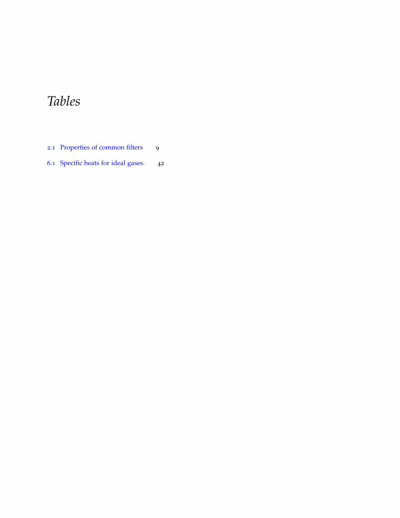
Tables
2.1 Properties of common filters 9
6.1 Specific heats for ideal gases. 42

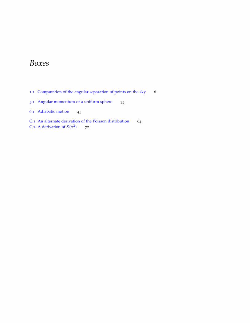
Boxes
1.1 Computation of the angular separation of points on the sky 6
5.1 Angular momentum of a uniform sphere 35
6.1 Adiabatic motion 43
C.1 An alternate derivation of the Poisson distribution 64
C.2 A derivation of E(σ2) 72

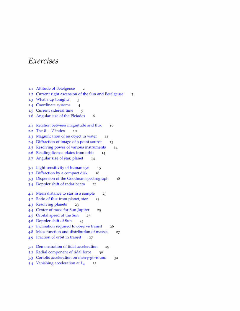
Exercises
1.1 Altitude of Betelgeuse 2
1.2 Current right ascension of the Sun and Betelgeuse 3
1.3 What’s up tonight? 3
1.4 Coordinate systems 4
1.5 Current sidereal time 5
1.6 Angular size of the Pleiades 6
2.1 Relation between magnitude and flux 10
2.2 The B−V index 10
2.3 Magnification of an object in water 11
2.4 Diffraction of image of a point source 13
2.5 Resolving power of various instruments 14
2.6 Reading license plates from orbit 14
2.7 Angular size of star, planet 14
3.1 Light sensitivity of human eye 15
3.2 Diffraction by a compact disk 18
3.3 Dispersion of the Goodman spectrograph 18
3.4 Doppler shift of radar beam 21
4.1 Mean distance to star in a sample 23
4.2 Ratio of flux from planet, star 23
4.3 Resolving planets 23
4.4 Center-of mass for Sun-Jupiter 25
4.5 Orbital speed of the Sun 25
4.6 Doppler shift of Sun 25
4.7 Inclination required to observe transit 26
4.8 Mass-function and distribution of masses 27
4.9 Fraction of orbit in transit 27
5.1 Demonstration of tidal acceleration 29
5.2 Radial component of tidal force 30
5.3 Coriolis acceleration on merry-go-round 32
5.4 Vanishing acceleration at L4 33
xiv
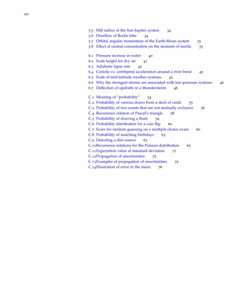
5.5 Hill radius of the Sun-Jupiter system 34
5.6 Overflow of Roche lobe 34
5.7 Orbital angular momentum of the Earth-Moon system 35
5.8 Effect of central concentration on the moment of inertia 35
6.1 Pressure increase in water 40
6.2 Scale height for dry air 41
6.3 Adiabatic lapse rate 42
6.4 Coriolis vs. centripetal acceleration around a river bend 45
6.5 Scale of mid-latitude weather systems 45
6.6 Why the strongest storms are associated with low-pressure systems 46
6.7 Deflection of updrafts in a thunderstorm 46
C.1 Meaning of “probability” 54
C.2 Probability of various draws from a deck of cards 55
C.3 Probability of two events that are not mutually exclusive 56
C.4 Recurrence relation of Pascal’s triangle 58
C.5 Probability of drawing a flush 59
C.6 Probability distribution for a coin flip 60
C.7 Score for random guessing on a multiple-choice exam 60
C.8 Probability of matching birthdays 63
C.9 Detecting a dim source 63
C.10Recurrence relations for the Poisson distribution 65
C.11Expectation value of standard deviation 71
C.12Propagation of uncertainties 75
C.13Examples of propagation of uncertainties 75
C.14Illustration of error in the mean 76
1Coordinates: Specifying Locations onthe Sky
1.1 Declination and right ascension
To talk about events in the sky, we need to specify where they arelocated. To specify where they are located, we need a point of refer-ence. This is a bit tricky: we are riding on the Earth, which rotatesand orbits the Sun; the Sun orbits the Milky Way; the Milky Waymoves through the Local Group; and on top of all this the universe isexpanding.
The primary criterion for choosing a coordinate system is con-venience. We want a system that is easy to use and that describesthe sky straightforwardly. As viewed from Earth, we appear to beat the center of a great sphere, with celestial objects lying on its sur-face. When describing locations on the Earth, we use two angles:latitude, which measures the angle north or south from the equator;and longitude, which measures the angle east or west from the primemeridian. Likewise, to describe the apparent position of objects onthis celestial sphere, we also need two angles.
NCP
SCP
Z
celestial equator δ
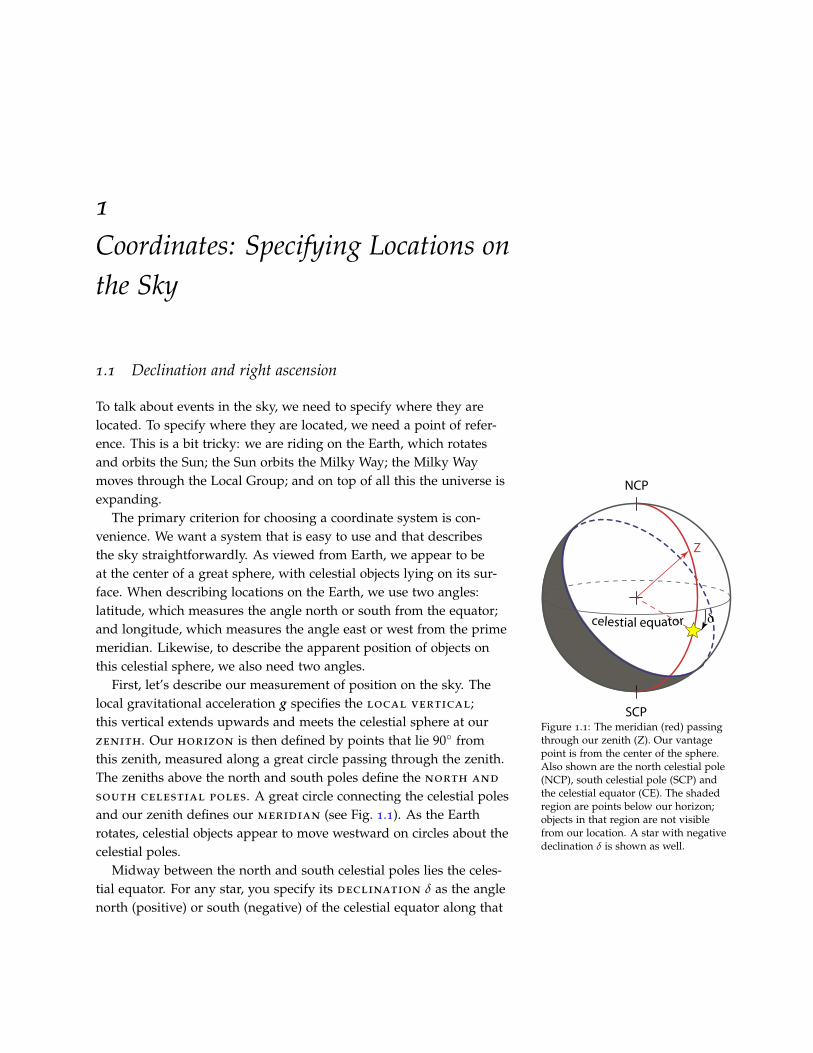
Figure 1.1: The meridian (red) passingthrough our zenith (Z). Our vantagepoint is from the center of the sphere.Also shown are the north celestial pole(NCP), south celestial pole (SCP) andthe celestial equator (CE). The shadedregion are points below our horizon;objects in that region are not visiblefrom our location. A star with negativedeclination δ is shown as well.
First, let’s describe our measurement of position on the sky. Thelocal gravitational acceleration g specifies the local vertical;this vertical extends upwards and meets the celestial sphere at ourzenith. Our horizon is then defined by points that lie 90 fromthis zenith, measured along a great circle passing through the zenith.The zeniths above the north and south poles define the north and
south celestial poles. A great circle connecting the celestial polesand our zenith defines our meridian (see Fig. 1.1). As the Earthrotates, celestial objects appear to move westward on circles about thecelestial poles.
Midway between the north and south celestial poles lies the celes-tial equator. For any star, you specify its declination δ as the anglenorth (positive) or south (negative) of the celestial equator along that
2 planets and telescopes
star’s meridian. For example, Betelgeuse, the red star in the shoulderof Orion, has a declination δ = 7 24′ 25′′. Polaris, the North star, hasδ = 89 15′ 51′′.Declination is quoted in degrees (),
arcminutes (′), and arcseconds (′′).There are 60 arcminutes in 1 degree and60 arcseconds in 1 arcminute. E X E R C I S E 1 . 1 — How far above our southern horizon will Betelgeuse
be when it crosses our meridian? Our latitude is 42 43′ 25′′N.Several of the exercises in this chapterrefer to the night sky as viewed frommid-Michigan in late January.
Declination measures how far north or south of the celestial equa-tor a given object lies. To specify an east-west location, we need an-other reference point. Because of the Earth’s rotation, we can’t use apoint on Earth, such as the Greenwich observatory (located on the 0
of longitude). We can, however, use the Earth’s motion around theSun: as the Earth moves around the Sun, the Sun appears to moveeastwards relative to the fixed stars. This path the Sun takes aroundthe celestial sphere is known as the ecliptic, and the constellationsthat lie along the ecliptic are the zodiac. Because the Earth’s rota-tional axis is tilted at an angle of 23 16′ with respect to its orbitalaxis, the Sun’s declination varies over the course of a year.
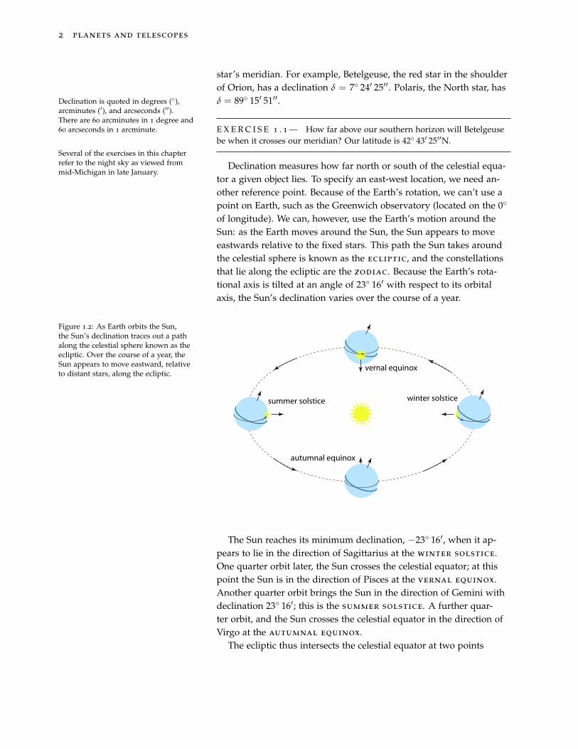
Figure 1.2: As Earth orbits the Sun,the Sun’s declination traces out a pathalong the celestial sphere known as theecliptic. Over the course of a year, theSun appears to move eastward, relativeto distant stars, along the ecliptic.
summer solstice
vernal equinox
autumnal equinox
winter solstice
The Sun reaches its minimum declination, −23 16′, when it ap-pears to lie in the direction of Sagittarius at the winter solstice.One quarter orbit later, the Sun crosses the celestial equator; at thispoint the Sun is in the direction of Pisces at the vernal equinox.Another quarter orbit brings the Sun in the direction of Gemini withdeclination 23 16′; this is the summer solstice. A further quar-ter orbit, and the Sun crosses the celestial equator in the direction ofVirgo at the autumnal equinox.
The ecliptic thus intersects the celestial equator at two points
coordinates: specifying locations on the sky 3
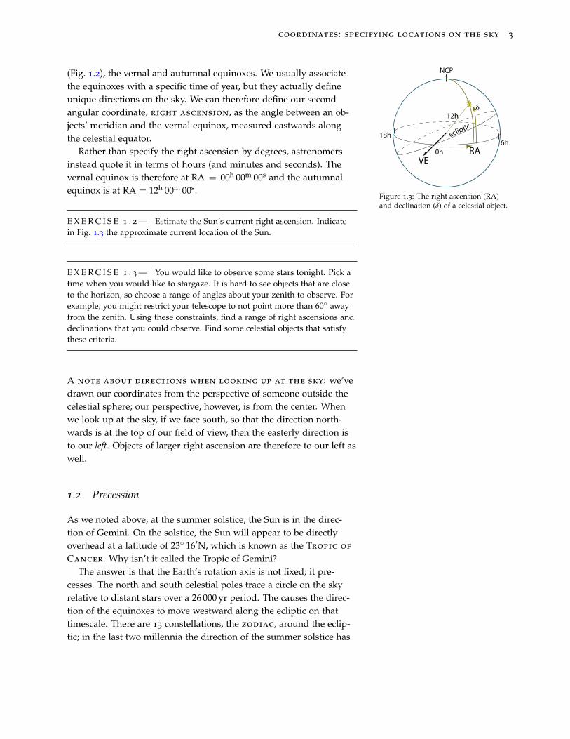
(Fig. 1.2), the vernal and autumnal equinoxes. We usually associatethe equinoxes with a specific time of year, but they actually defineunique directions on the sky. We can therefore define our secondangular coordinate, right ascension, as the angle between an ob-jects’ meridian and the vernal equinox, measured eastwards alongthe celestial equator.
VERA0h
12h
18h6h
ecliptic
δ
NCP
Figure 1.3: The right ascension (RA)and declination (δ) of a celestial object.
Rather than specify the right ascension by degrees, astronomersinstead quote it in terms of hours (and minutes and seconds). Thevernal equinox is therefore at RA = 00h 00m 00s and the autumnalequinox is at RA = 12h 00m 00s.
E X E R C I S E 1 . 2 — Estimate the Sun’s current right ascension. Indicatein Fig. 1.3 the approximate current location of the Sun.
E X E R C I S E 1 . 3 — You would like to observe some stars tonight. Pick atime when you would like to stargaze. It is hard to see objects that are closeto the horizon, so choose a range of angles about your zenith to observe. Forexample, you might restrict your telescope to not point more than 60 awayfrom the zenith. Using these constraints, find a range of right ascensions anddeclinations that you could observe. Find some celestial objects that satisfythese criteria.
A note about directions when looking up at the sky: we’vedrawn our coordinates from the perspective of someone outside thecelestial sphere; our perspective, however, is from the center. Whenwe look up at the sky, if we face south, so that the direction north-wards is at the top of our field of view, then the easterly direction isto our left. Objects of larger right ascension are therefore to our left aswell.
1.2 Precession
As we noted above, at the summer solstice, the Sun is in the direc-tion of Gemini. On the solstice, the Sun will appear to be directlyoverhead at a latitude of 23 16′N, which is known as the Tropic of
Cancer. Why isn’t it called the Tropic of Gemini?The answer is that the Earth’s rotation axis is not fixed; it pre-
cesses. The north and south celestial poles trace a circle on the skyrelative to distant stars over a 26 000 yr period. The causes the direc-tion of the equinoxes to move westward along the ecliptic on thattimescale. There are 13 constellations, the zodiac, around the eclip-tic; in the last two millennia the direction of the summer solstice has
4 planets and telescopes
shifted one constellation over, from Cancer to Gemini. Likewise, thewinter solstice used to be in the direction of Capricorn; now it is inthe direction of Sagittarius.
As a practical matter, this means that the coordinates of right as-cension and declination, which are based on the direction of theEarth’s rotation axis, slowly change. To account for this, when giv-ing the coordinates for an object astronomers specify an epoch—areference time to which the right ascension and declination refer.The current epoch is J2000, which refers to roughly noon UTC on 1
January 2000.
E X E R C I S E 1 . 4 — Brainstorm some possible coordinate systems, anddescribe their advantages and disadvantages in comparison to rightascension and declination.
1.3 Keeping time
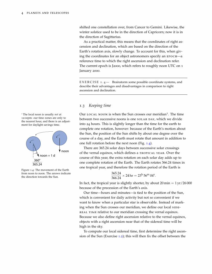
Our local noon is when the Sun crosses our meridian1. The time1 The local noon is usually not at12:00pm: our time zones are only tothe nearest hour, and there is an adjust-ment for daylight savings time.
between two successive noons is one solar day, which we divideinto 24 hours. This is slightly longer than the time for the earth tocomplete one rotation, however: because of the Earth’s motion aboutthe Sun, the position of the Sun shifts by about one degree over thecourse of a day, and the Earth must rotate that amount in addition toone full rotation before the next noon (Fig. 1.4).
360°365.24
noonnoon + 1 d
Figure 1.4: The movement of the Earthfrom noon to noon. The arrows indicatethe direction towards the Sun.
There are 365.24 solar days between successive solar crossingsof the vernal equinox, which defines a tropical year. Over thecourse of this year, the extra rotation on each solar day adds up toone complete rotation of the Earth. The Earth rotates 366.24 times inone tropical year, and therefore the rotation period of the Earth is
365.24366.24
× 24 hr = 23h 56m 04s.
In fact, the tropical year is slightly shorter, by about 20 min = 1 yr/26 000because of the precession of the Earth’s axis.
Our time—hours and minutes—is tied to the position of the Sun,which is convenient for daily activity but not so convenient if wewant to know when a particular star is observable. Instead of mark-ing when the Sun crosses our meridian, we define our local side-real time relative to our meridian crossing the vernal equinox.Because we also define right ascension relative to the vernal equinox,objects with a right ascension near that of the sidereal time will behigh in the sky.
To compute our local sidereal time, first determine the right ascen-sion of the Sun (Exercise 1.2); this will then fix the offset between the
coordinates: specifying locations on the sky 5
local sidereal time and the local noon in UTC. We can then computeour offset for local noon based on our longitude.
E X E R C I S E 1 . 5 — Local noon at 0 longitude corresponds to 12:00 UTC.Given that our longitude is 84 28′ 33′′W, what is our local noontime in UTC.What local time would this correspond to today? From this and yourestimate of the Sun’s current hour angle, what is the current sidereal time?
1.4 Parallax
The motion of the Earth around the Sun does cause a small shift inthe apparent angular position of a star, a phenomena known as par-allax. This effect is exploited to determine the distance to nearbystars.
1 AU
d
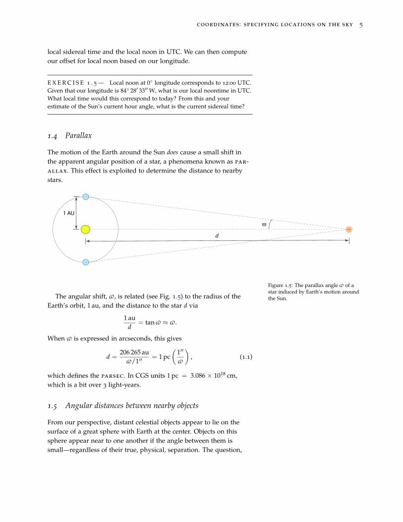
ϖ
Figure 1.5: The parallax angle v of astar induced by Earth’s motion aroundthe Sun.The angular shift, v, is related (see Fig. 1.5) to the radius of the
Earth’s orbit, 1 au, and the distance to the star d via
1 aud
= tan v ≈ v.
When v is expressed in arcseconds, this gives
d =206 265 au
v/1′′= 1 pc
(1′′
v
), (1.1)
which defines the parsec. In CGS units 1 pc = 3.086 × 1018 cm,which is a bit over 3 light-years.
1.5 Angular distances between nearby objects
From our perspective, distant celestial objects appear to lie on thesurface of a great sphere with Earth at the center. Objects on thissphere appear near to one another if the angle between them issmall—regardless of their true, physical, separation. The question,
6 planets and telescopes
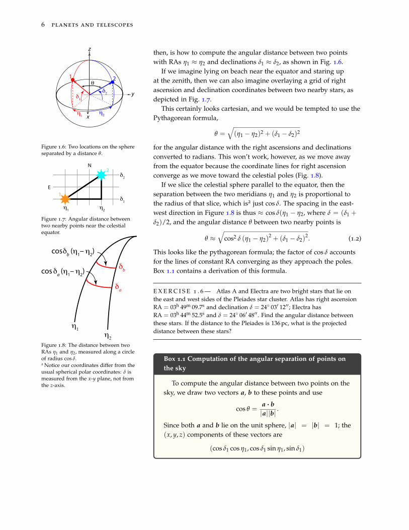
then, is how to compute the angular distance between two pointswith RAs η1 ≈ η2 and declinations δ1 ≈ δ2, as shown in Fig. 1.6.
x
z
y
η1
η2
δ2
δ1
θ1 2
Figure 1.6: Two locations on the sphereseparated by a distance θ.
If we imagine lying on beach near the equator and staring upat the zenith, then we can also imagine overlaying a grid of rightascension and declination coordinates between two nearby stars, asdepicted in Fig. 1.7.
N
E
η1 η2
δ2
δ1
1
2
Figure 1.7: Angular distance betweentwo nearby points near the celestialequator.
This certainly looks cartesian, and we would be tempted to use thePythagorean formula,
θ =√(η1 − η2)2 + (δ1 − δ2)2
for the angular distance with the right ascensions and declinationsconverted to radians. This won’t work, however, as we move awayfrom the equator because the coordinate lines for right ascensionconverge as we move toward the celestial poles (Fig. 1.8).
η1
δa
δb
η2
cosδb (η1– η2)
cosδa (η1– η2)
Figure 1.8: The distance between twoRAs η1 and η2, measured along a circleof radius cos δ.
If we slice the celestial sphere parallel to the equator, then theseparation between the two meridians η1 and η2 is proportional tothe radius of that slice, which is2 just cos δ. The spacing in the east-
2 Notice our coordinates differ from theusual spherical polar coordinates: δ ismeasured from the x-y plane, not fromthe z-axis.
west direction in Figure 1.8 is thus ≈ cos δ(η1 − η2, where δ = (δ1 +
δ2)/2, and the angular distance θ between two nearby points is
θ ≈√
cos2 δ (η1 − η2)2 + (δ1 − δ2)
2. (1.2)
This looks like the pythagorean formula; the factor of cos δ accountsfor the lines of constant RA converging as they approach the poles.Box 1.1 contains a derivation of this formula.
E X E R C I S E 1 . 6 — Atlas A and Electra are two bright stars that lie onthe east and west sides of the Pleiades star cluster. Atlas has right ascensionRA = 03h 49m 09.7s and declination δ = 24 03′ 12′′; Electra hasRA = 03h 44m 52.5s and δ = 24 06′ 48′′. Find the angular distance betweenthese stars. If the distance to the Pleiades is 136 pc, what is the projecteddistance between these stars?
Box 1.1 Computation of the angular separation of points onthe sky
To compute the angular distance between two points on thesky, we draw two vectors a, b to these points and use
cos θ =a · b|a||b| .
Since both a and b lie on the unit sphere, |a| = |b| = 1; the(x, y, z) components of these vectors are
(cos δ1 cos η1, cos δ1 sin η1, sin δ1)
coordinates: specifying locations on the sky 7
Box 1.1 continued
and(cos δ2 cos η2, cos δ2 sin η2, sin δ2) ,
respectively. Taking the dot product,
cos θ = cos δ1 cos δ2 (cos η1 cos η2 + sin η1 sin η2) + sin δ1 sin δ2
= cos δ1 cos δ2 cos (η1 − η2) + sin δ1 sin δ2. (1.3)
We make heavy use of the sine and cosine addition formula:cos(x + y) = cos x cos y − sin x sin y, and sin(−y) = − sin y,cos(−x) = cos(x). See Appendix B for a refresher.
We are usually interested in the angular distance betweentwo nearby sources. We can therefore use the expansion rule,
cos x ≈ 1− x2
2, x 1
on θ and η1 − η2 in equation (1.3):
1− θ2
2≈ cos δ1 cos δ2
[1− (η1 − η2)
2
2
]+ sin δ1 sin δ2
= cos(δ1 − δ2)− cos δ1 cos δ2(η1 − η2)
2
2.
We can now expand cos(δ1 − δ2), cancel common factors andmultiply by 2,
θ2 ≈ (δ1 − δ2)2 + cos δ1 cos δ2(η1 − η2)
2.
Next, we write δ1 = δ + ∆, δ2 = δ − ∆, where δ = (δ1 + δ2)/2and ∆ = (δ1 − δ2)/2 are the average and difference of the twodeclinations. Inserting these into cos δ1 cos δ2 and expandinggives
cos δ1 cos δ2 = cos2 δ cos2 ∆− sin2 δ sin2 ∆.
Expanding cos ∆ ≈ 1− ∆2/2 and sin ∆ ≈ ∆ and keeping termsto O(∆2) gives
cos δ1 cos δ2 ≈ cos2 δ− ∆2
so to lowest order in (δ1 − δ2) and (η1 − η2),
θ2 ≈ (δ1 − δ2)2 + cos2 δ(η2
1 − η22)
which is eq. (1.2).

2Light and Telescopes
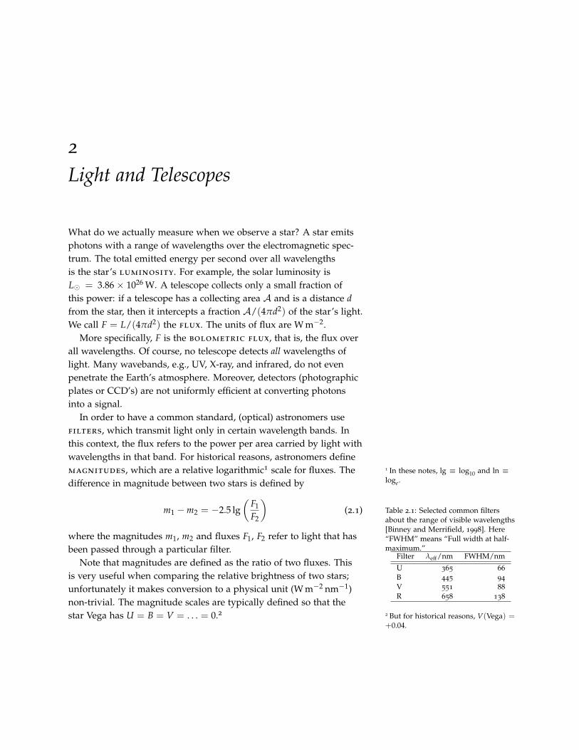
What do we actually measure when we observe a star? A star emitsphotons with a range of wavelengths over the electromagnetic spec-trum. The total emitted energy per second over all wavelengthsis the star’s luminosity. For example, the solar luminosity isL = 3.86 × 1026 W. A telescope collects only a small fraction ofthis power: if a telescope has a collecting area A and is a distance dfrom the star, then it intercepts a fraction A/(4πd2) of the star’s light.We call F = L/(4πd2) the flux. The units of flux are W m−2.
More specifically, F is the bolometric flux, that is, the flux overall wavelengths. Of course, no telescope detects all wavelengths oflight. Many wavebands, e.g., UV, X-ray, and infrared, do not evenpenetrate the Earth’s atmosphere. Moreover, detectors (photographicplates or CCD’s) are not uniformly efficient at converting photonsinto a signal.
In order to have a common standard, (optical) astronomers usefilters, which transmit light only in certain wavelength bands. Inthis context, the flux refers to the power per area carried by light withwavelengths in that band. For historical reasons, astronomers definemagnitudes, which are a relative logarithmic1 scale for fluxes. The 1 In these notes, lg ≡ log10 and ln ≡
loge.difference in magnitude between two stars is defined by
m1 −m2 = −2.5 lg(
F1
F2
)(2.1)
where the magnitudes m1, m2 and fluxes F1, F2 refer to light that hasbeen passed through a particular filter.
Table 2.1: Selected common filtersabout the range of visible wavelengths[Binney and Merrifield, 1998]. Here“FWHM” means “Full width at half-maximum.”
Filter λeff/nm FWHM/nm
U 365 66
B 445 94
V 551 88
R 658 138
Note that magnitudes are defined as the ratio of two fluxes. Thisis very useful when comparing the relative brightness of two stars;unfortunately it makes conversion to a physical unit (W m−2 nm−1)non-trivial. The magnitude scales are typically defined so that thestar Vega has U = B = V = . . . = 0.2 2 But for historical reasons, V(Vega) =
+0.04.
10 planets and telescopes
E X E R C I S E 2 . 1 —
1. Suppose we have two identical stars, A and B. Star A is twice as far awayas star B. What is mA −mB?
2. Suppose a star’s luminosity changes by a tiny amount δ. What is thecorresponding change in that stars’ magnitude?
If we take a ratio of two magnitudes using different fil-ters from a single star, then we have a rough measure of thestar’s color. This ratio is called a color index. For example,
B−V ≡ mB −mV = −2.5 lgFBFV
gives a measure for how blue the star’s spectrum appears.
E X E R C I S E 2 . 2 — Which has the larger B−V index: a red star, likeBetelgeuse, or a blue-white star, like Rigel?
Two stars with the same apparent brightness may have verydifferent intrinsic brightnesses: one may be very dim and nearby, theother very luminous and faraway. To compare intrinsic brightness,we need to correct for the distance to the star3. We define the dis-3 This assumes we know the distance,
which can be difficult!tance modulus as the difference in magnitude between a given starand the magnitude it would have if it were at a distance of 10 pc:
DM ≡ m−m(10 pc) = −2.5 lg[
L4πd2
4π(10 pc)2
L
]= −2.5 lg
(10 pc
d
)2
= 5 lg(
dpc
)− 5.
The magnitude that the star would have if it were at 10 pc distance iscalled its absolute magnitude, M ≡ m−DM.
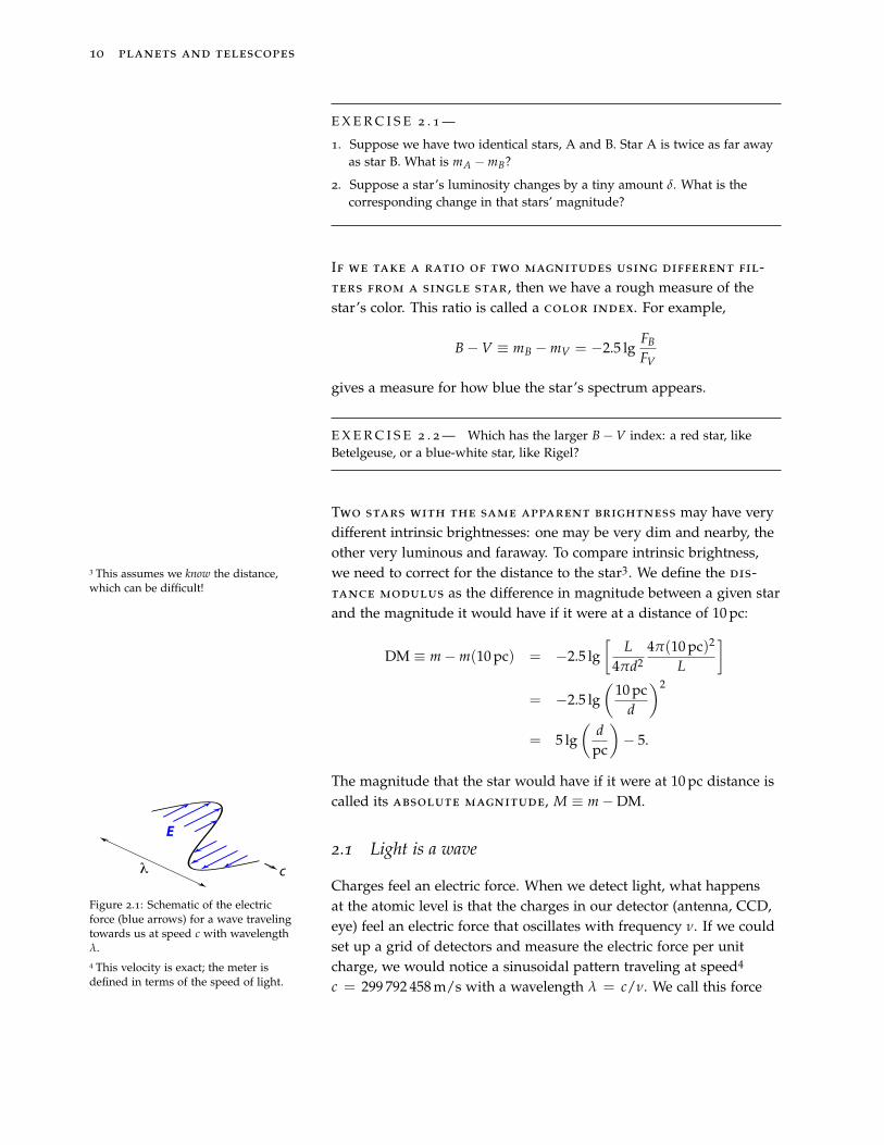
2.1 Light is a wavecλ
E
Figure 2.1: Schematic of the electricforce (blue arrows) for a wave travelingtowards us at speed c with wavelengthλ.
Charges feel an electric force. When we detect light, what happensat the atomic level is that the charges in our detector (antenna, CCD,eye) feel an electric force that oscillates with frequency ν. If we couldset up a grid of detectors and measure the electric force per unitcharge, we would notice a sinusoidal pattern traveling at speed44 This velocity is exact; the meter is
defined in terms of the speed of light. c = 299 792 458 m/s with a wavelength λ = c/ν. We call this force
light and telescopes 11
per charge the electric field E(x, t). The intensity of the light at ourdetector is proportional to |E|2.
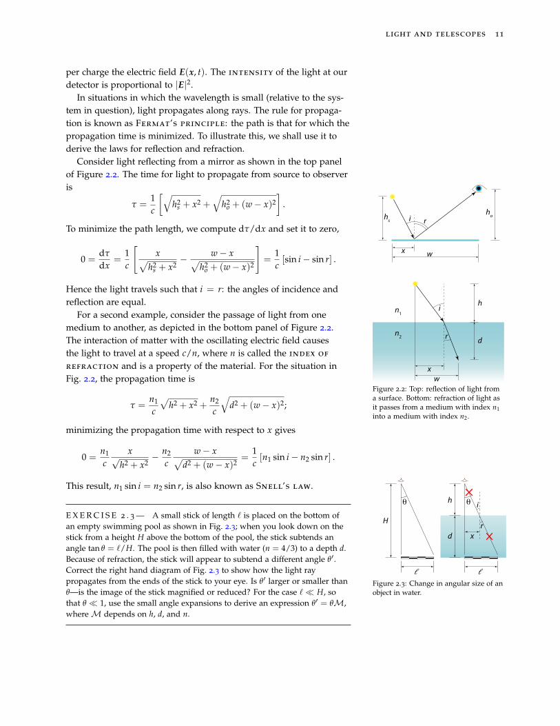
In situations in which the wavelength is small (relative to the sys-tem in question), light propagates along rays. The rule for propaga-tion is known as Fermat’s principle: the path is that for which thepropagation time is minimized. To illustrate this, we shall use it toderive the laws for reflection and refraction.
Consider light reflecting from a mirror as shown in the top panelof Figure 2.2. The time for light to propagate from source to observeris
τ =1c
[√h2
s + x2 +√
h2o + (w− x)2
].
To minimize the path length, we compute dτ/dx and set it to zero,
0 =dτ
dx=
1c
[x√
h2s + x2
− w− x√h2
o + (w− x)2
]=
1c[sin i− sin r] .
Hence the light travels such that i = r: the angles of incidence andreflection are equal.
ri
w
hs
in1
n2 r
ho
x
d
h
wx
Figure 2.2: Top: reflection of light froma surface. Bottom: refraction of light asit passes from a medium with index n1into a medium with index n2.
For a second example, consider the passage of light from onemedium to another, as depicted in the bottom panel of Figure 2.2.The interaction of matter with the oscillating electric field causesthe light to travel at a speed c/n, where n is called the index of
refraction and is a property of the material. For the situation inFig. 2.2, the propagation time is
τ =n1
c
√h2 + x2 +
n2
c
√d2 + (w− x)2;
minimizing the propagation time with respect to x gives
0 =n1
cx√
h2 + x2− n2
cw− x√
d2 + (w− x)2=
1c[n1 sin i− n2 sin r] .
This result, n1 sin i = n2 sin r, is also known as Snell’s law.
θ
H
θ
x
h
d
i
r
Figure 2.3: Change in angular size of anobject in water.
E X E R C I S E 2 . 3 — A small stick of length ` is placed on the bottom ofan empty swimming pool as shown in Fig. 2.3; when you look down on thestick from a height H above the bottom of the pool, the stick subtends anangle tan θ = `/H. The pool is then filled with water (n = 4/3) to a depth d.Because of refraction, the stick will appear to subtend a different angle θ′.Correct the right hand diagram of Fig. 2.3 to show how the light raypropagates from the ends of the stick to your eye. Is θ′ larger or smaller thanθ—is the image of the stick magnified or reduced? For the case ` H, sothat θ 1, use the small angle expansions to derive an expression θ′ = θM,whereM depends on h, d, and n.
12 planets and telescopes
2.2 Diffraction
A telescope makes an image by focusing the incoming rays of lightonto a detector. Suppose we are at a fixed point and the wave ispropagating past us. In general we would observe an electric fieldamplitude of the form
E(t) = A0 cos (2πνt) + B0 sin (2πνt)
where ν = c/λ is the frequency. Let’s check this: in going from t = 0to t = T = 1/ν, the period of the wave, the argument of the cosineand sine goes from 0 to 2π, which is one oscillation. To find the netintensity I from a number of waves, we sum the amplitudes to getthe net electric field E and then take the square |E|2.
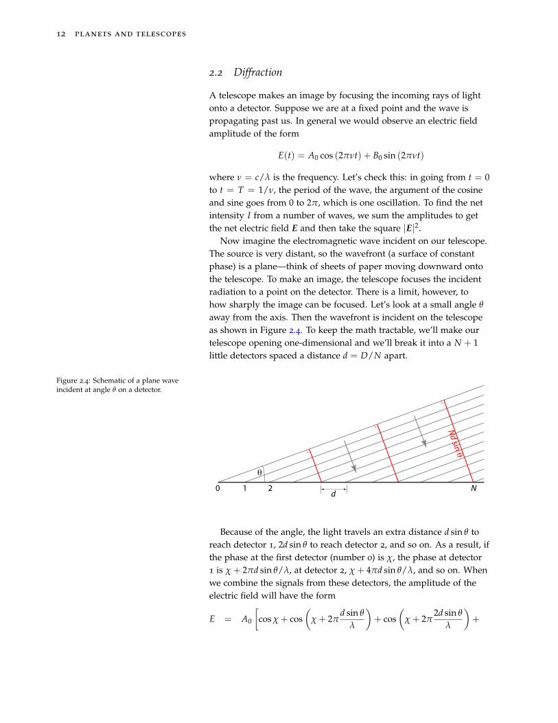
Now imagine the electromagnetic wave incident on our telescope.The source is very distant, so the wavefront (a surface of constantphase) is a plane—think of sheets of paper moving downward ontothe telescope. To make an image, the telescope focuses the incidentradiation to a point on the detector. There is a limit, however, tohow sharply the image can be focused. Let’s look at a small angle θ
away from the axis. Then the wavefront is incident on the telescopeas shown in Figure 2.4. To keep the math tractable, we’ll make ourtelescope opening one-dimensional and we’ll break it into a N + 1little detectors spaced a distance d = D/N apart.
Figure 2.4: Schematic of a plane waveincident at angle θ on a detector.
10 2 N
Nd sin θ
d
θ
Because of the angle, the light travels an extra distance d sin θ toreach detector 1, 2d sin θ to reach detector 2, and so on. As a result, ifthe phase at the first detector (number 0) is χ, the phase at detector1 is χ + 2πd sin θ/λ, at detector 2, χ + 4πd sin θ/λ, and so on. Whenwe combine the signals from these detectors, the amplitude of theelectric field will have the form
E = A0
[cos χ + cos
(χ + 2π
d sin θ
λ
)+ cos
(χ + 2π
2d sin θ
λ
)+
light and telescopes 13
+ cos(
χ + 2π3d sin θ
λ
)+ . . . + cos
(χ + 2π
Nd sin θ
λ
)]+B0
[sin χ + sin
(χ + 2π
d sin θ
λ
)+ . . . + sin
(χ + 2π
Nd sin θ
λ
)].
When θ → 0, the amplitude goes to E → (N + 1) [A0 cos χ + B0 sin χ],and so the brightness I(θ → 0) = |E|2 is a very large number. That’sgood: the light from the star is focused to a point. Now, how largedoes θ have to be before E goes to zero?
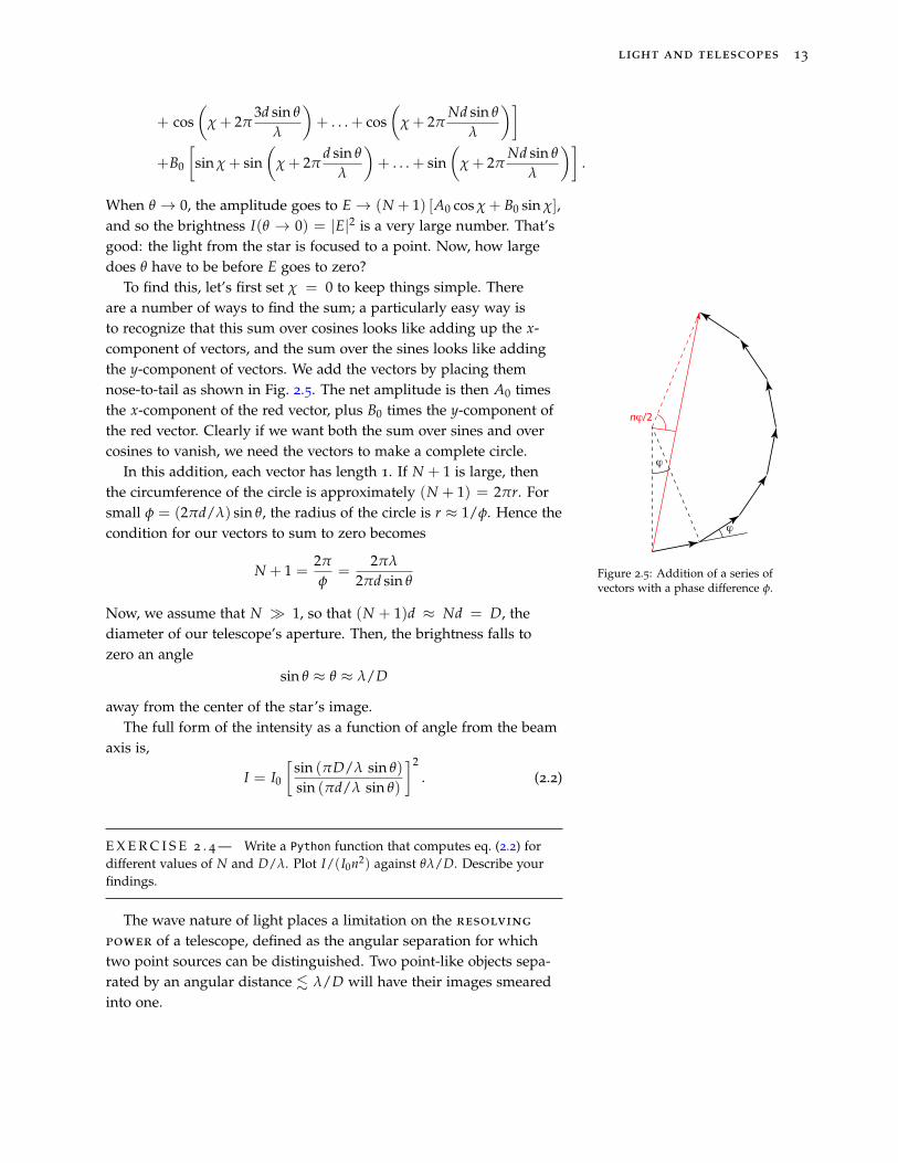
To find this, let’s first set χ = 0 to keep things simple. Thereare a number of ways to find the sum; a particularly easy way isto recognize that this sum over cosines looks like adding up the x-component of vectors, and the sum over the sines looks like addingthe y-component of vectors. We add the vectors by placing themnose-to-tail as shown in Fig. 2.5. The net amplitude is then A0 timesthe x-component of the red vector, plus B0 times the y-component ofthe red vector. Clearly if we want both the sum over sines and overcosines to vanish, we need the vectors to make a complete circle.
ϕ
ϕ
nϕ/2
Figure 2.5: Addition of a series ofvectors with a phase difference φ.
In this addition, each vector has length 1. If N + 1 is large, thenthe circumference of the circle is approximately (N + 1) = 2πr. Forsmall φ = (2πd/λ) sin θ, the radius of the circle is r ≈ 1/φ. Hence thecondition for our vectors to sum to zero becomes
N + 1 =2π
φ=
2πλ
2πd sin θ
Now, we assume that N 1, so that (N + 1)d ≈ Nd = D, thediameter of our telescope’s aperture. Then, the brightness falls tozero an angle
sin θ ≈ θ ≈ λ/D
away from the center of the star’s image.The full form of the intensity as a function of angle from the beam
axis is,
I = I0
[sin (πD/λ sin θ)
sin (πd/λ sin θ)
]2. (2.2)
E X E R C I S E 2 . 4 — Write a Python function that computes eq. (2.2) fordifferent values of N and D/λ. Plot I/(I0n2) against θλ/D. Describe yourfindings.
The wave nature of light places a limitation on the resolving
power of a telescope, defined as the angular separation for whichtwo point sources can be distinguished. Two point-like objects sepa-rated by an angular distance . λ/D will have their images smearedinto one.
14 planets and telescopes
E X E R C I S E 2 . 5 — What is the resolving power of the Hubble SpaceTelescope (D = 2.4 m) and the Keck telescope (D = 10 m) at a wavelengthλ = 570 nm? Estimate the angular resolution of the human eye at thatwavelength. What is the resolving power of the Arecibo radio telescope(D = 305 m) at a frequency of 3 GHz?
E X E R C I S E 2 . 6 — It is often claimed that some agencies have thetechnological capability to read license plates from satellites. Evaluate thisclaim: for a telescope in low-Earth orbit, how large an aperture would berequired to resolve the lettering on a license plate? Could Hubble (2.4 maperture) do this? Use your best guess the orbital altitude and letter size, butjustify your reasoning.
For ground-based telescopes, an even more severe limitation is therefraction of light by the atmosphere. The atmosphere is turbulent,and the swirling eddies contain variations in density that change therefractive index and distort the wavefront. This distortion smears theimage over an angular scale that is typically larger than 1′′.
E X E R C I S E 2 . 7 — What is the angular size of a solar-sized star(R = 6.96× 10⁵ km) at a distance of 1 pc? What is the angular size of Mars(R = 3 390 km) at a distance of 0.5 au? How would the difference in angularsize affect the appearance of these two objects?
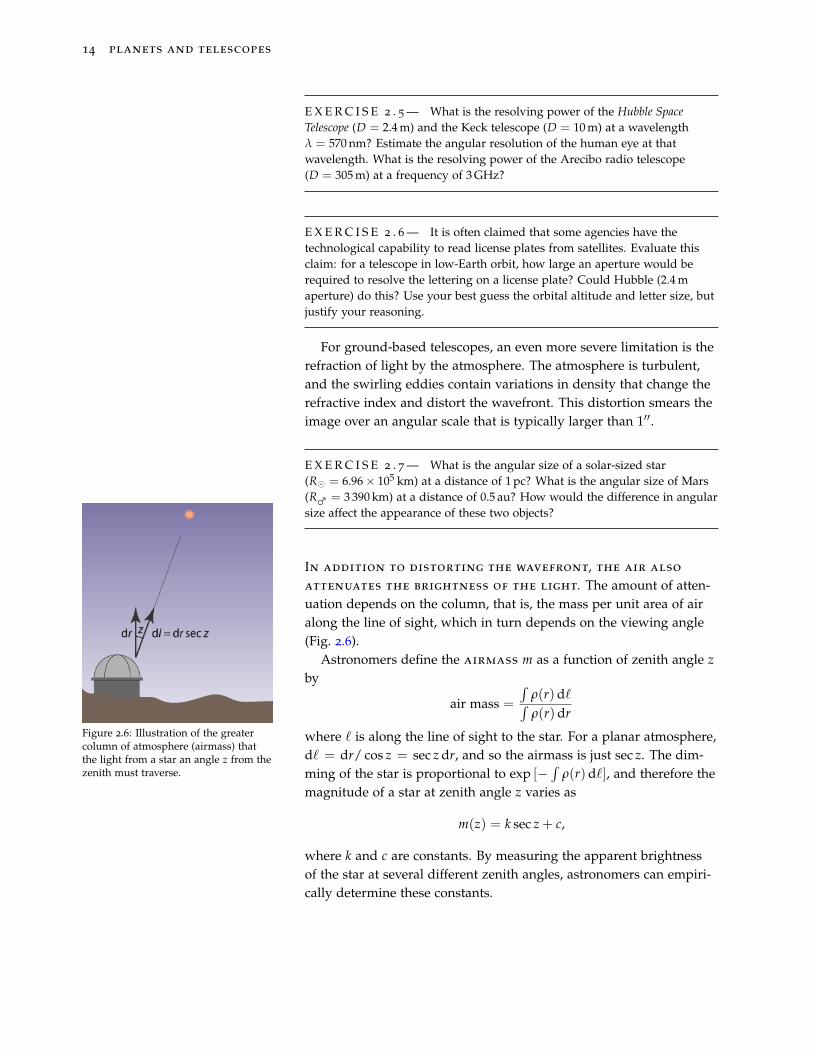
In addition to distorting the wavefront, the air also
attenuates the brightness of the light. The amount of atten-uation depends on the column, that is, the mass per unit area of airalong the line of sight, which in turn depends on the viewing angle(Fig. 2.6).
Figure 2.6: Illustration of the greatercolumn of atmosphere (airmass) thatthe light from a star an angle z from thezenith must traverse.
Astronomers define the airmass m as a function of zenith angle zby
air mass =
∫ρ(r)d`∫ρ(r)dr
where ` is along the line of sight to the star. For a planar atmosphere,d` = dr/ cos z = sec z dr, and so the airmass is just sec z. The dim-ming of the star is proportional to exp [−
∫ρ(r)d`], and therefore the
magnitude of a star at zenith angle z varies as
m(z) = k sec z + c,
where k and c are constants. By measuring the apparent brightnessof the star at several different zenith angles, astronomers can empiri-cally determine these constants.
3Spectroscopy
3.1 Electromagnetic radiation is quantized
Electromagnetic radiation—light—is carried by massless particlesknown as photons. Being massless, they travel at a speed c in allframes. The energy of a photon depends on its frequency ν: Eν = hν.Since ν = λ/c, we can also express the energy of a photon as Eλ =
hc/λ. When matter absorbs or emits radiant energy, it does so byabsorbing or emitting photons.
E X E R C I S E 3 . 1 — On a very dark night, the eye can make out starsdown to visual magnitude V ≈ 6. Given that the sun has V = −26.71 andthat the flux from the sun in V-band is approximately 103 W/m2, estimatethe radiant flux from this V = 6 star. If the V band photons have an averageλ = 550 nm, how many photons from this barely visible star enter your pupiland strike your retina each second?
Suppose we shine a monochromatic (i.e., comprising a singlewavelength) beam of light at a tinted piece of glass (sunglasses,for example). The light that emerges on the other side is the samecolor—meaning it has the same wavelength—but is dimmer. Whatare we to make of this? For the exiting light to be dimmer, some ofthe photons must have been absorbed. But if the photons are indis-tinguishable, why are only some absorbed? Once we have quantiza-tion, we are forced to adopt a probabilistic viewpoint: each photonhas a certain probability of being absorbed.
3.2 The hydrogen atom
The electrons bound to an atom or molecule can only occupy stateshaving a discrete set of energies. For example, the electron in a hy-
16 planets and telescopes
drogen atom only has energies
En = −13.6 eV× 1n2 , (3.1)
where n > 0 is an integer known as the principal quantum number.These energies are negative, relative to a free electron. For example, ittakes 13.6 eV to remove an electron in its ground state from the atom.
Because the electrons in an atom can only have certain energies,the atom can only absorb or emit light at specific wavelengths, suchthat the energy of the photon matches the difference in energy be-tween two levels. For example, a hydrogen atom can absorb a photonof energy
E1→2 = −13.6 eV(
122 −
112
)= 10.2 eV
corresponding to the energy required to move the electron fromn = 1 to n = 2.
The wavelengths that can be emitted or absorbed by a hydro-gen atom at rest can be found by substituting E = hc/λ into equa-tion (3.1):
λm→n = λ0
(1n2 −
1m2
)−1, (3.2)
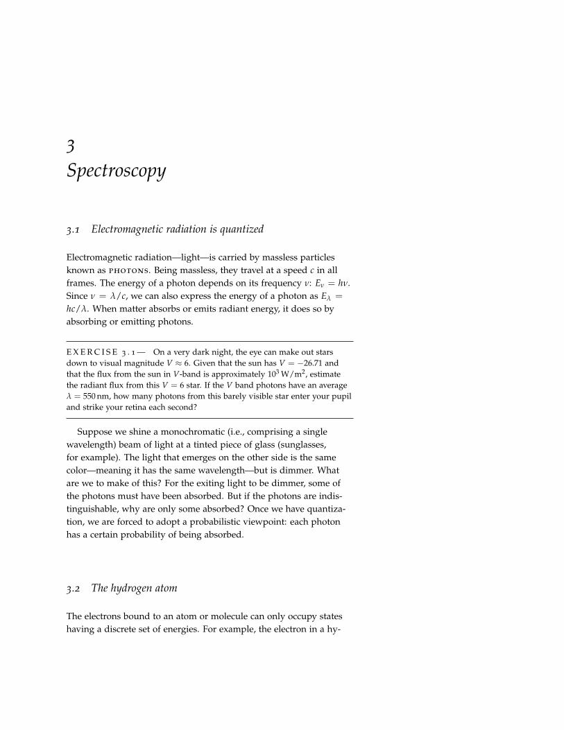
where λ0 = 91.2 nm. The transitions to the lowest levels are namedafter their discoverers: Lyman for m → 1, Balmer for m → 2, Paschenfor m → 3. A greek letter is used to denote the higher state: for ex-ample Lyman α (abbr. Lyα) means 2 → 1, with λLyα = 121.6 nm. Thefirst line transition in the Balmer series is 3 → 2, and is designatedHα: λHα = 656.3 nm. The first 50 lines for the Lyman (m→ 1), Balmer(m → 2), and Paschen (m → 3) are shown in Fig. 3.1; note the 4 → 3transition is outside the plot range.
Figure 3.1: Spectral lines of neutralhydrogen.
200 400 600 800 1000 1200 1400
(nm)
Lym
an (
)
Balm
er
()
Pasc
hen (
)
spectroscopy 17
3.3 Diffraction Gratings
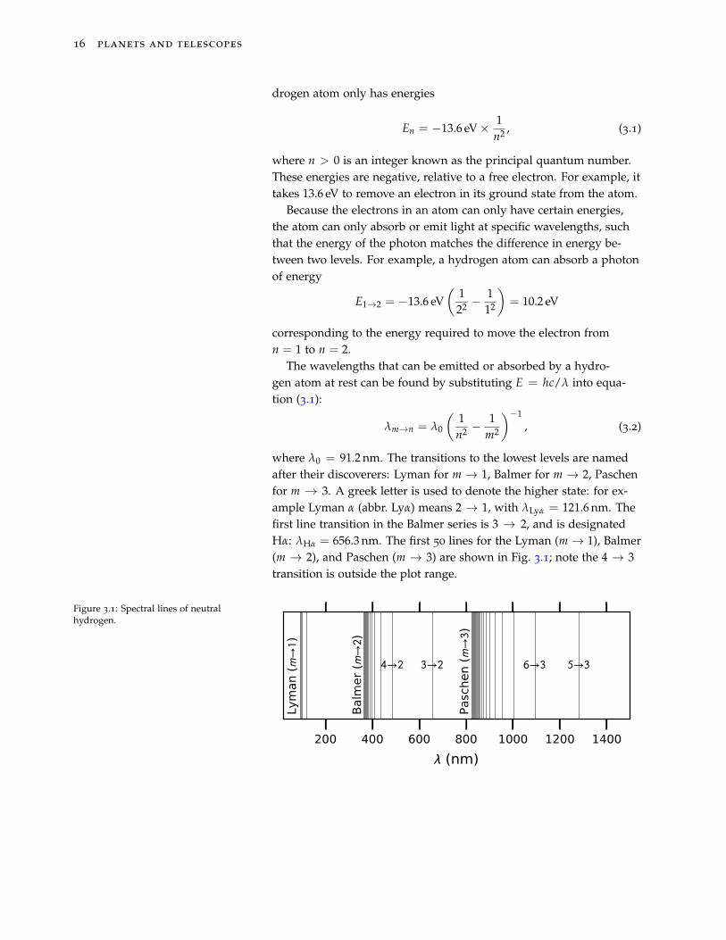
To look at the different wavelengths in the light from a source, weuse a diffraction grating, which is a series of fine, closely spaced linesetched on a surface. When light is projected onto the grating, it isreflected from the lines in all directions. Along a given direction, thelight from two adjacent lines will travel a slightly different distance:if the spacing between lines is d, the extra distance traveled from aneighboring line is d sin θ, where θ is the angle between the incidentand reflected rays. Because of this different path length, a distant de-tector will in general receive waves of many different phases. Whenthe waves are added together, the peaks and troughs cancel, and theresult is that the summed wave is greatly reduced in amplitude.
There are, however, certain directions along which the intensity ismaximized. If the extra path length is a multiple of the wavelengththen all the rays reach the distant detector with the same phase, sothe intensity is bright. That is, at angles satisfying
d sin θ = mλ, (3.3)
bright spots are produced.This situation is depicted in Fig. 3.2 form = 1. For each line, the path length differs by one wavelength fromits neighbors; as a result, the rays along a direction θ (at the right ofthe figure) are in phase. Since different wavelengths produce theirbright spots at different angles, the light is dispersed in wavelength,producing a spectrum. A good home example of a grating is a com-pact disk: the tracks on the disk act as the grating.
θ
d
d sinθ
Figure 3.2: A diffraction grating.
18 planets and telescopes
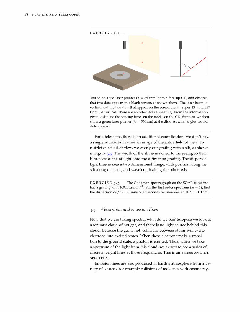
E X E R C I S E 3 . 2 —
θ
You shine a red laser pointer (λ = 650 nm) onto a face-up CD, and observethat two dots appear on a blank screen, as shown above. The laser beam isvertical and the two dots that appear on the screen are at angles 23 and 52
from the vertical. There are no other dots appearing. From the informationgiven, calculate the spacing between the tracks on the CD. Suppose we thenshine a green laser pointer (λ = 530 nm) at the disk. At what angles woulddots appear?
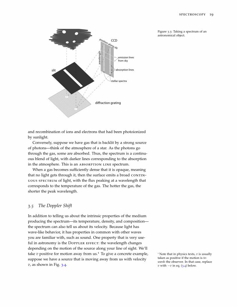
For a telescope, there is an additional complication: we don’t havea single source, but rather an image of the entire field of view. Torestrict our field of view, we overly our grating with a slit, as shownin Figure 3.3. The width of the slit is matched to the seeing so thatif projects a line of light onto the diffraction grating. The dispersedlight thus makes a two dimensional image, with position along theslit along one axis, and wavelength along the other axis.
E X E R C I S E 3 . 3 — The Goodman spectrograph on the SOAR telescopehas a grating with 400 lines mm−1. For the first order spectrum (m = 1), findthe dispersion dθ/dλ, in units of arcseconds per nanometer, at λ = 500 nm.
3.4 Absorption and emission lines
Now that we are taking spectra, what do we see? Suppose we look ata tenuous cloud of hot gas, and there is no light source behind thiscloud. Because the gas is hot, collisions between atoms will exciteelectrons into excited states. When these electrons make a transi-tion to the ground state, a photon is emitted. Thus, when we takea spectrum of the light from this cloud, we expect to see a series ofdiscrete, bright lines at those frequencies. This is an emission line
spectrum.Emission lines are also produced in Earth’s atmosphere from a va-
riety of sources: for example collisions of molecues with cosmic rays
spectroscopy 19
diraction grating
CCD
slit
stellar spectra
absorption lines
emission linesfrom sky
position along slit
wav
elen
gth
Figure 3.3: Taking a spectrum of anastronomical object.
and recombination of ions and electrons that had been photoionizedby sunlight.
Conversely, suppose we have gas that is backlit by a strong sourceof photons—think of the atmosphere of a star. As the photons gothrough the gas, some are absorbed. Thus, the spectrum is a continu-ous blend of light, with darker lines corresponding to the absorptionin the atmosphere. This is an absorption line spectrum.
When a gas becomes sufficiently dense that it is opaque, meaningthat no light gets through it, then the surface emits a broad contin-uous spectrum of light, with the flux peaking at a wavelength thatcorresponds to the temperature of the gas. The hotter the gas, theshorter the peak wavelength.
3.5 The Doppler Shift
In addition to telling us about the intrinsic properties of the mediumproducing the spectrum—its temperature, density, and composition—the spectrum can also tell us about its velocity. Because light haswave-like behavior, it has properties in common with other wavesyou are familiar with, such as sound. One property that is very use-ful in astronomy is the Doppler effect: the wavelength changesdepending on the motion of the source along your line of sight. We’lltake v positive for motion away from us.1 To give a concrete example, 1 Note that in physics texts, v is usually
taken as positive if the motion is to-wards the observer. In that case, replacev with −v in eq. (3.4) below.
suppose we have a source that is moving away from us with velocityv, as shown in Fig. 3.4.
20 planets and telescopes
vT
λ+vT
λ
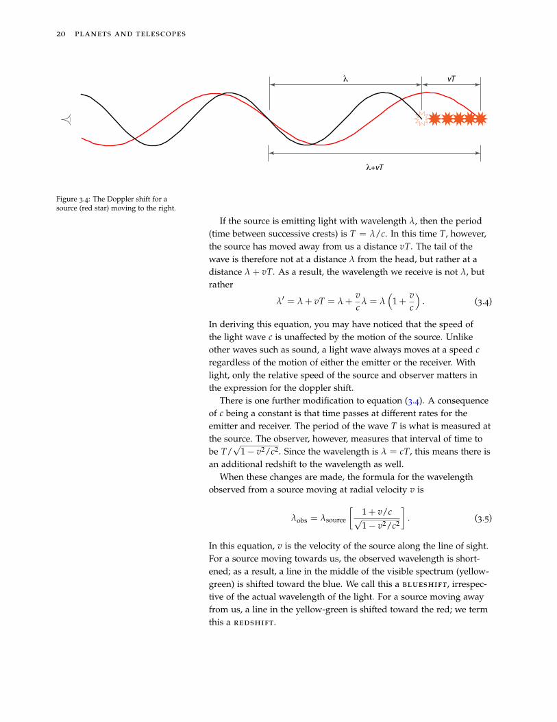
Figure 3.4: The Doppler shift for asource (red star) moving to the right.
If the source is emitting light with wavelength λ, then the period(time between successive crests) is T = λ/c. In this time T, however,the source has moved away from us a distance vT. The tail of thewave is therefore not at a distance λ from the head, but rather at adistance λ + vT. As a result, the wavelength we receive is not λ, butrather
λ′ = λ + vT = λ +vc
λ = λ(
1 +vc
). (3.4)
In deriving this equation, you may have noticed that the speed ofthe light wave c is unaffected by the motion of the source. Unlikeother waves such as sound, a light wave always moves at a speed cregardless of the motion of either the emitter or the receiver. Withlight, only the relative speed of the source and observer matters inthe expression for the doppler shift.
There is one further modification to equation (3.4). A consequenceof c being a constant is that time passes at different rates for theemitter and receiver. The period of the wave T is what is measured atthe source. The observer, however, measures that interval of time tobe T/
√1− v2/c2. Since the wavelength is λ = cT, this means there is
an additional redshift to the wavelength as well.When these changes are made, the formula for the wavelength
observed from a source moving at radial velocity v is
λobs = λsource
[1 + v/c√1− v2/c2
]. (3.5)
In this equation, v is the velocity of the source along the line of sight.For a source moving towards us, the observed wavelength is short-ened; as a result, a line in the middle of the visible spectrum (yellow-green) is shifted toward the blue. We call this a blueshift, irrespec-tive of the actual wavelength of the light. For a source moving awayfrom us, a line in the yellow-green is shifted toward the red; we termthis a redshift.
spectroscopy 21
E X E R C I S E 3 . 4 — A radar detector used by law enforcement measuresspeed by emitting a radar beam with frequency 22 GHz and measuring thefrequency of the reflected signal.
1. What is the wavelength λ of the radar beam?
2. If a motorist is going 40 m/s (about 89 miles/hour) away from the officer,what is ∆λ = λmotorist − λofficer? What is ∆λ/λ?

4Detection of Exoplanets
4.1 The Difficulty with Direct Detection
Suppose we want to observe exoplanets directly. Let’s first estimatehow far we have to look.
E X E R C I S E 4 . 1 — The density of stars in the solar neighborhood is0.14 pc−3. Suppose 50% of the stars have planets, and we want a sample ofabout 20 planetary systems. What would be the radius (in parsec) of thevolume containing this many systems? Given this radius, what is the averagedistance to a star in this sample?
Next let’s estimate the difference in brightness between a planetand its host star. We shall use our solar system as an example.
E X E R C I S E 4 . 2 — The Sun, which is at a distance of 1 au, has anapparent V-band magnitude V = −26.74. At its closest approach ofapproximately 4 au, Jupiter has an apparent magnitude VX = −2.94.Compute the ratio of fluxes in V-band, i.e., FX/F, if both Jupiter and theSun were at the same distance.
Finally, we know that there is a limit to the angular resolution of atelescope. This limit is imposed by both the atmospheric seeing andthe telescope optics. Let’s estimate how the angular separation ofplanet and star compares with a fiducial angular resolution.
E X E R C I S E 4 . 3 — Jupiter’s mean distance from the Sun is 5.2 au.Suppose we were to view the Sun-Jupiter system from the average distancederived in exercise 4.1; what would be the angular separation betweenJupiter and the Sun? How does this compare with the atmospheric seeingunder good conditions?
As these exercises illustrate, imaging a planet directly is a daunt-ing task. Astronomers have therefore resorted to indirect means, in
24 planets and telescopes
which the host star is observed to vary due to the influence of theplanet’s gravitational force. This motivates a review of Kepler’s prob-lem.
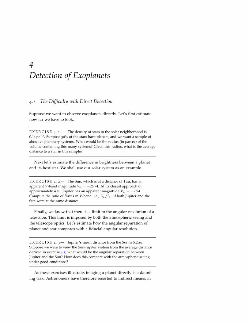
4.2 Planetary Orbits: Kepler
Suppose we have a exoplanet system with a planet p and a star s.The vector from the star to the planet is rsp = rp − rs, and the forcethat the star exerts on the planet is
Fsp = −GMp Ms
|rsp|3rsp. (4.1)
The planet exerts a force on the star Fps = −Fsp.To make this problem more tractable, we shall put the origin of
our coordinate system at the center of mass, as shown in Fig. 4.1,
O
mp
ms
rprs
rsp = rp-rs
O
R
mp
ms
xp
xs
Figure 4.1: Center of mass in a star-planet system.
R =Msrs + Mprp
Ms + Mp;
in this frame the star and planet have positions
xs = rs − R = −Mp
Mp + Msrsp (4.2)
xp = rp − R =Ms
Mp + Msrsp (4.3)
and hence accelerations
d2xs
dt2 = −Mp
Mp + Ms
d2rsp
dt2
d2xp
dt2 =Ms
Mp + Ms
d2rsp
dt2 .
If we substitute this acceleration into the equation of motion forthe planet,
Mpd2xp
dt2 = Fsp,
and use eq. (4.1) for Fsp, we get the reduced equation of motion
d2rsp
dt2 = −GMs + Mp
|rsp|3rsp. (4.4)
We recover this same equation if we substitute the accelerations intothe equation of motion for the star. Hence for a two body problem,we only need to solve equation (4.4) for rsp(t) and then use equa-tions (4.2) and (4.3) to compute the positions xs(t), xp(t) of the starand planet.
detection of exoplanets 25
E X E R C I S E 4 . 4 — Locate the center of mass for the Sun-Jupiter system:
MMX
= 1047; rX = 5.2 au.
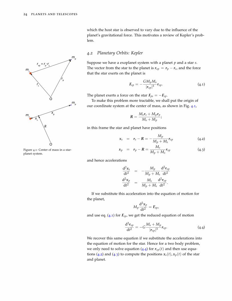
The solution to equation (4.4) is an elliptical orbit (Fig. 4.2) withthe center-of-force at one focus of the ellipse. The period T dependson the semi-major axis a of the ellipse,
T2 =4π2
G(Ms + Mp)a3. (4.5)
Suppose the orbit is circular, so that |rsp| = a is constant. Then bycombining equations (4.5) and (4.2) we can find the orbital speed ofthe star,
vs =Mp
Ms + Mp× 2πa
T=
[GMp
aMp
Ms + Mp
]1/2. (4.6)
This speed is detectable via doppler shift of the stellar absorptionlines.
f
a ea
Figure 4.2: Orbital elements for a bodymoving in a gravitational potentialabout a fixed center of force, indicatedby the yellow star.
E X E R C I S E 4 . 5 — Compute the orbital speed of the Sun for thetwo-body Sun-Jupiter system;
MMX
= 1047; rX = 5.2 au.
E X E R C I S E 4 . 6 — What is the wavelength shift induced by the motionof the Sun, computed in exercise 4.5, for an absorption line with restwavelength 600 nm?
4.3 Transits
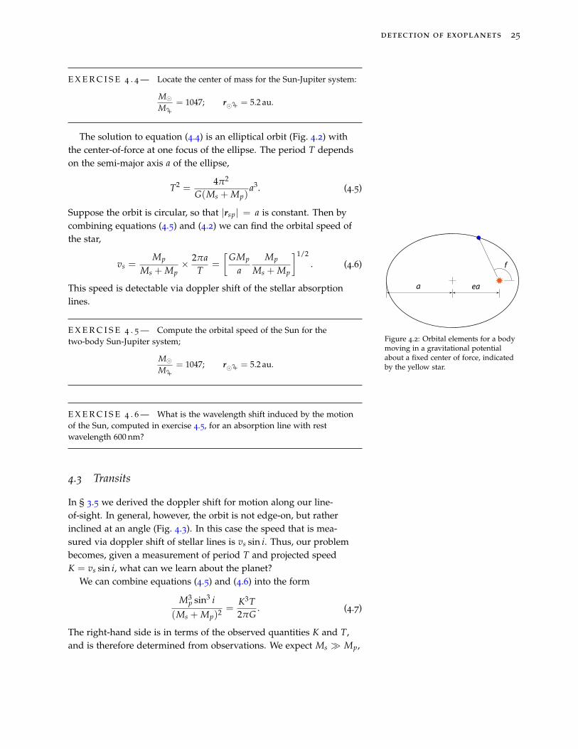
In § 3.5 we derived the doppler shift for motion along our line-of-sight. In general, however, the orbit is not edge-on, but ratherinclined at an angle (Fig. 4.3). In this case the speed that is mea-sured via doppler shift of stellar lines is vs sin i. Thus, our problembecomes, given a measurement of period T and projected speedK = vs sin i, what can we learn about the planet?
We can combine equations (4.5) and (4.6) into the form
M3p sin3 i
(Ms + Mp)2 =K3T2πG
. (4.7)
The right-hand side is in terms of the observed quantities K and T,and is therefore determined from observations. We expect Ms Mp,
26 planets and telescopes
Figure 4.3: Schematic of the inclinationof a planetary orbit to our line of sight.
i
and can usually estimate Ms from spectroscopy of the star. Even withthis information, we can only determine Mp sin i.
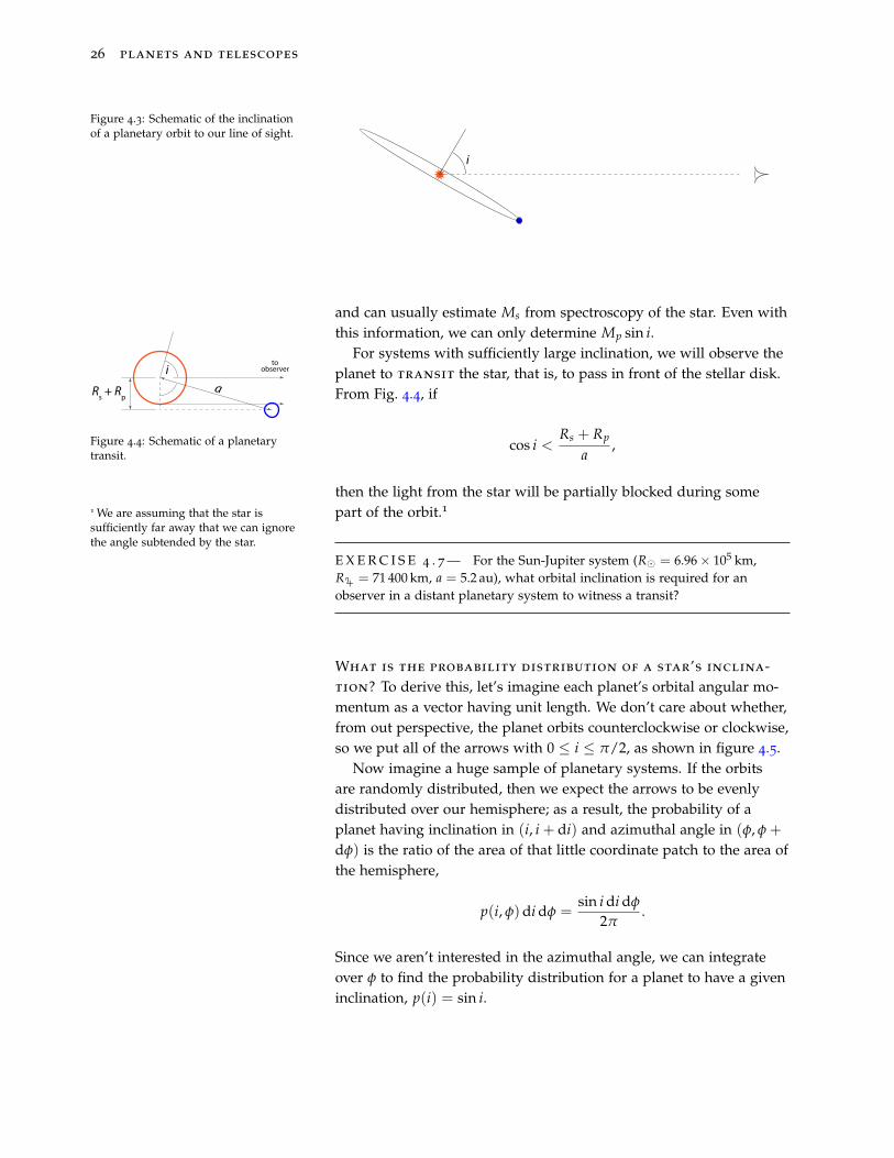
For systems with sufficiently large inclination, we will observe theplanet to transit the star, that is, to pass in front of the stellar disk.From Fig. 4.4, ifaRs + Rp
ito
observer
Figure 4.4: Schematic of a planetarytransit.
cos i <Rs + Rp
a,
then the light from the star will be partially blocked during somepart of the orbit.11 We are assuming that the star is
sufficiently far away that we can ignorethe angle subtended by the star.
E X E R C I S E 4 . 7 — For the Sun-Jupiter system (R = 6.96× 10⁵ km,RX = 71 400 km, a = 5.2 au), what orbital inclination is required for anobserver in a distant planetary system to witness a transit?
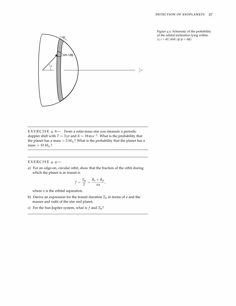
What is the probability distribution of a star’s inclina-tion? To derive this, let’s imagine each planet’s orbital angular mo-mentum as a vector having unit length. We don’t care about whether,from out perspective, the planet orbits counterclockwise or clockwise,so we put all of the arrows with 0 ≤ i ≤ π/2, as shown in figure 4.5.
Now imagine a huge sample of planetary systems. If the orbitsare randomly distributed, then we expect the arrows to be evenlydistributed over our hemisphere; as a result, the probability of aplanet having inclination in (i, i + di) and azimuthal angle in (φ, φ +
dφ) is the ratio of the area of that little coordinate patch to the area ofthe hemisphere,
p(i, φ)di dφ =sin i di dφ
2π.
Since we aren’t interested in the azimuthal angle, we can integrateover φ to find the probability distribution for a planet to have a giveninclination, p(i) = sin i.
detection of exoplanets 27
i
di
sin i dφ
Figure 4.5: Schematic of the probabilityof the orbital inclination lying within(i, i + di) and (φ, φ + dφ).
E X E R C I S E 4 . 8 — From a solar-mass star you measure a periodicdoppler shift with T = 3 yr and K = 18 m s−1. What is the probability thatthe planet has a mass > 2 MX? What is the probability that the planet has amass > 10 MX?
E X E R C I S E 4 . 9 —
a) For an edge-on, circular orbit, show that the fraction of the orbit duringwhich the planet is in transit is
f =Ttr
T=
Rs + Rp
πa,
where a is the orbital separation.
b) Derive an expression for the transit duration Ttr in terms of a and themasses and radii of the star and planet.
c) For the Sun-Jupiter system, what is f and Ttr?

5Beyond Kepler’s Laws
When we studied the two-body problem, we treated the masses assimple points. In reality, they are complex extended objects. In thischapter, we’ll explore some of the effects that arise when we go be-yond the simple problem of two massive point particles orbiting oneanother.
5.1 Tidal forces
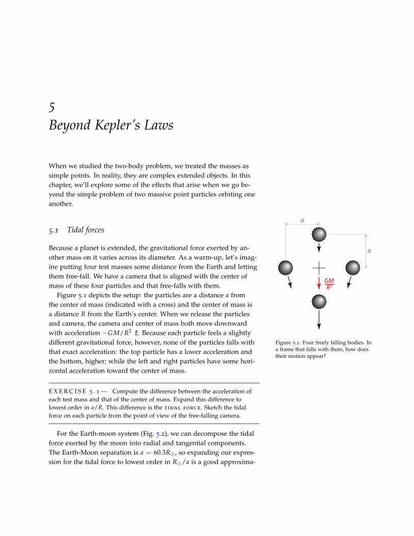
Because a planet is extended, the gravitational force exerted by an-other mass on it varies across its diameter. As a warm-up, let’s imag-ine putting four test masses some distance from the Earth and lettingthem free-fall. We have a camera that is aligned with the center ofmass of these four particles and that free-falls with them.
a
a
GMR2
Figure 5.1: Four freely falling bodies. Ina frame that falls with them, how doestheir motion appear?
Figure 5.1 depicts the setup: the particles are a distance a fromthe center of mass (indicated with a cross) and the center of mass isa distance R from the Earth’s center. When we release the particlesand camera, the camera and center of mass both move downwardwith acceleration −GM/R2 z. Because each particle feels a slightlydifferent gravitational force, however, none of the particles falls withthat exact acceleration: the top particle has a lower acceleration andthe bottom, higher; while the left and right particles have some hori-zontal acceleration toward the center of mass.
E X E R C I S E 5 . 1 — Compute the difference between the acceleration ofeach test mass and that of the center of mass. Expand this difference tolowest order in a/R. This difference is the tidal force. Sketch the tidalforce on each particle from the point of view of the free-falling camera.
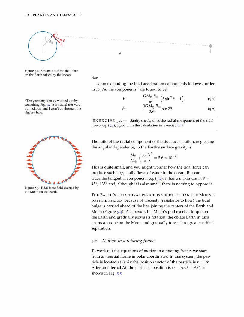
For the Earth-moon system (Fig. 5.2), we can decompose the tidalforce exerted by the moon into radial and tangential components.The Earth-Moon separation is a = 60.3R⊕, so expanding our expres-sion for the tidal force to lowest order in R⊕/a is a good approxima-
30 planets and telescopes
θ F
Fr
Fθ
R⊕
a
Figure 5.2: Schematic of the tidal forceon the Earth raised by the Moon.
tion.Upon expanding the tidal acceleration components to lowest order
in R⊕/a, the components1 are found to be
1 The geometry can be worked out byconsulting Fig. 5.2; it is straightforward,but tedious, and I won’t go through thealgebra here.
r :GM$R⊕
a3
(3 sin2 θ − 1
)(5.1)
θ :3GM$R⊕
2a3 sin 2θ. (5.2)
E X E R C I S E 5 . 2 — Sanity check: does the radial component of the tidalforce, eq. (5.1), agree with the calculation in Exercise 5.1?
Figure 5.3: Tidal force field exerted bythe Moon on the Earth.
The ratio of the radial component of the tidal acceleration, neglectingthe angular dependence, to the Earth’s surface gravity is
M$M⊕
(R⊕a
)3= 5.6× 10⁻⁸.
This is quite small, and you might wonder how the tidal force canproduce such large daily flows of water in the ocean. But con-sider the tangential component, eq. (5.2): it has a maximum at θ =
45, 135 and, although it is also small, there is nothing to oppose it.
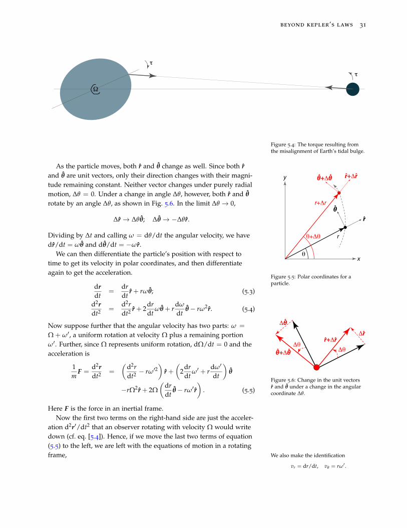
The Earth’s rotational period is shorter than the Moon’sorbital period. Because of viscosity (resistance to flow) the tidalbulge is carried ahead of the line joining the centers of the Earth andMoon (Figure 5.4). As a result, the Moon’s pull exerts a torque onthe Earth and gradually slows its rotation; the oblate Earth in turnexerts a torque on the Moon and gradually forces it to greater orbitalseparation.
5.2 Motion in a rotating frame
To work out the equations of motion in a rotating frame, we startfrom an inertial frame in polar coordinates. In this system, the par-ticle is located at (r, θ); the position vector of the particle is r = rr.After an internal ∆t, the particle’s position is (r + ∆r, θ + ∆θ), asshown in Fig. 5.5.
beyond kepler’s laws 31
τ
Ω
τ
Figure 5.4: The torque resulting fromthe misalignment of Earth’s tidal bulge.
y
xθ
θ+Δθ
θ+Δθ
θ
r+Δr
r
r
r+Δr
Figure 5.5: Polar coordinates for aparticle.
As the particle moves, both r and θ change as well. Since both rand θ are unit vectors, only their direction changes with their magni-tude remaining constant. Neither vector changes under purely radialmotion, ∆θ = 0. Under a change in angle ∆θ, however, both r and θ
rotate by an angle ∆θ, as shown in Fig. 5.6. In the limit ∆θ → 0,
∆r → ∆θθ; ∆θ→ −∆θr.
Dividing by ∆t and calling ω = dθ/dt the angular velocity, we havedr/dt = ωθ and dθ/dt = −ωr.
ΔθΔθ
ΔθΔr
θ+Δθ
r+Δr
Figure 5.6: Change in the unit vectorsr and θ under a change in the angularcoordinate ∆θ.
We can then differentiate the particle’s position with respect totime to get its velocity in polar coordinates, and then differentiateagain to get the acceleration.
drdt
=drdt
r + rωθ; (5.3)
d2rdt2 =
d2rdt2 r + 2
drdt
ωθ+ rdω
dtθ− rω2r. (5.4)
Now suppose further that the angular velocity has two parts: ω =
Ω + ω′, a uniform rotation at velocity Ω plus a remaining portionω′. Further, since Ω represents uniform rotation, dΩ/dt = 0 and theacceleration is
1m
F =d2rdt2 =
(d2rdt2 − rω′2
)r +
(2
drdt
ω′ + rdω′
dt
)θ
−rΩ2r + 2Ω(
drdt
θ− rω′ r)
. (5.5)
Here F is the force in an inertial frame.Now the first two terms on the right-hand side are just the acceler-
ation d2r′/dt2 that an observer rotating with velocity Ω would writedown (cf. eq. [5.4]). Hence, if we move the last two terms of equation(5.5) to the left, we are left with the equations of motion in a rotatingframe, We also make the identification
vr = dr/dt, vθ = rω′.
32 planets and telescopes
d2r′
dt2 =1m
Frot =1m
F + rΩ2r︸ ︷︷ ︸centrifugal
+ 2Ω(vθ r− vrθ
)︸ ︷︷ ︸Coriolis
. (5.6)
The centrifugal force is outwards (along r); the Coriolis forcedepends on velocity and deflects the motion of a particle at rightangles to its velocity2. If you’ve ever tried to walk in a straight line on2 That is, if you are moving in the r
direction, the Coriolis force is in the θdirection, and vice versa.
a spinning merry-go-round, then you’ve met the Coriolis force.
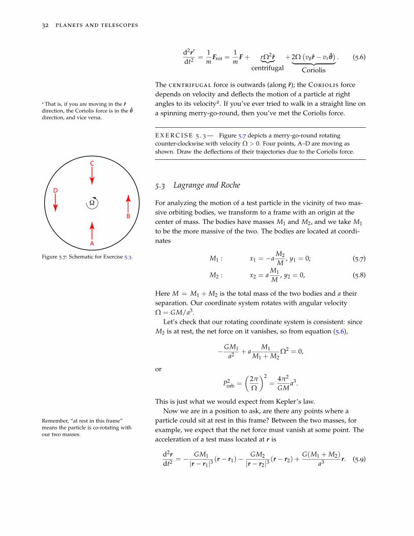
E X E R C I S E 5 . 3 — Figure 5.7 depicts a merry-go-round rotatingcounter-clockwise with velocity Ω > 0. Four points, A–D are moving asshown. Draw the deflections of their trajectories due to the Coriolis force.
Ω
A
B
C
D
Figure 5.7: Schematic for Exercise 5.3.
5.3 Lagrange and Roche
For analyzing the motion of a test particle in the vicinity of two mas-sive orbiting bodies, we transform to a frame with an origin at thecenter of mass. The bodies have masses M1 and M2, and we take M1
to be the more massive of the two. The bodies are located at coordi-nates
M1 : x1 = −aM2
M, y1 = 0; (5.7)
M2 : x2 = aM1
M, y2 = 0, (5.8)
Here M = M1 + M2 is the total mass of the two bodies and a theirseparation. Our coordinate system rotates with angular velocityΩ = GM/a3.
Let’s check that our rotating coordinate system is consistent: sinceM2 is at rest, the net force on it vanishes, so from equation (5.6),
−GM1
a2 + aM1
M1 + M2Ω2 = 0,
or
P2orb =
(2π
Ω
)2=
4π2
GMa3.
This is just what we would expect from Kepler’s law.Now we are in a position to ask, are there any points where a
particle could sit at rest in this frame? Between the two masses, forRemember, “at rest in this frame”means the particle is co-rotating withour two masses.
example, we expect that the net force must vanish at some point. Theacceleration of a test mass located at r is
d2rdt2 = − GM1
|r− r1|3(r− r1)−
GM2
|r− r2|3(r− r2) +
G(M1 + M2)
a3 r. (5.9)
beyond kepler’s laws 33
Along the x-axis, points where a particle would feel no accelerationare given by the roots of the equations
x < x1 :GM1
(x1 − x)2 +GM2
(x2 − x)2 +G(M1 + M2)
a3 x = 0;
x1 < x < x2 : − GM1
(x− x1)2 +GM2
(x2 − x)2 +G(M1 + M2)
a3 x = 0;
x2 < x :GM1
(x− x1)2 +GM2
(x− x2)2 +G(M1 + M2)
a3 x = 0.
This is a nasty quintic equation; if, however, we take the limit M2 M1 then after some inspired algebra we find that there are threeroots, which are the first three Lagrange points:
L1 xL1 ≈ a
M1
M1 + M2−[
M2
3(M1 + M2)
]1/3
;
L2 xL2 ≈ a
M1
M1 + M2+
[M2
3(M1 + M2)
]1/3
;
L3 xL3 ≈ a−M1 + 2M2
M1 + M2+
7M2
12M1
.
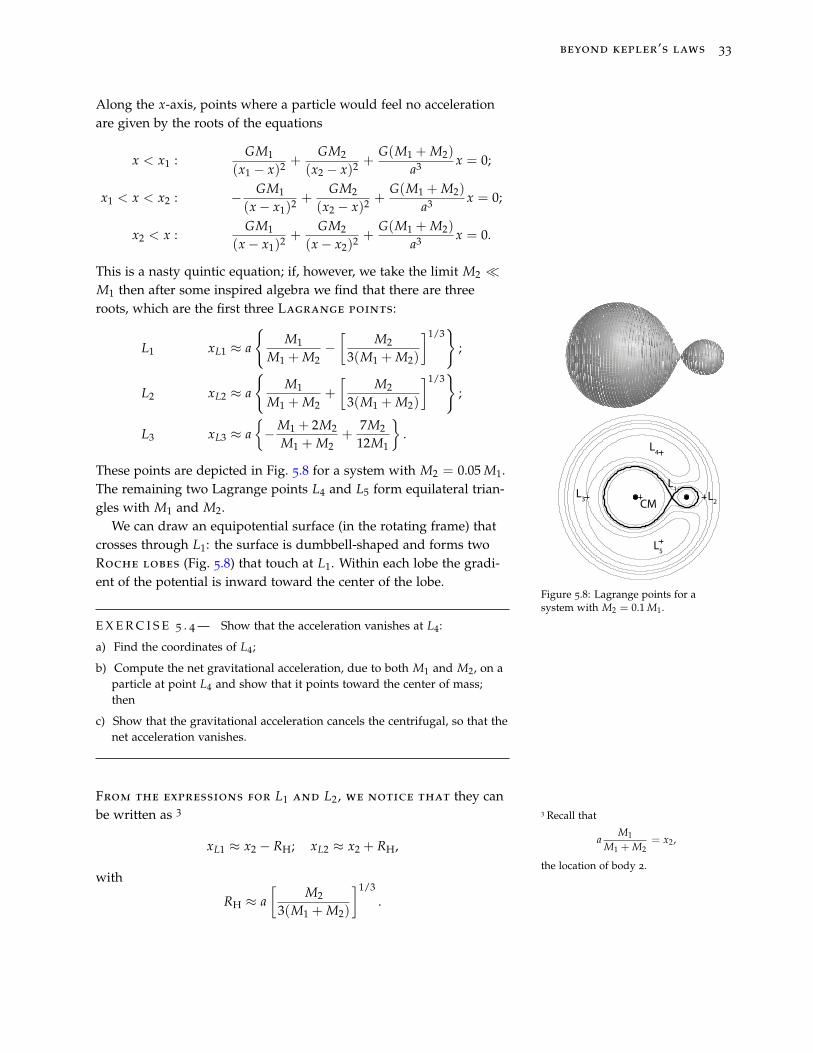
These points are depicted in Fig. 5.8 for a system with M2 = 0.05 M1.The remaining two Lagrange points L4 and L5 form equilateral trian-gles with M1 and M2. CM
L4
L5
L2L3L1
Figure 5.8: Lagrange points for asystem with M2 = 0.1 M1.
We can draw an equipotential surface (in the rotating frame) thatcrosses through L1: the surface is dumbbell-shaped and forms twoRoche lobes (Fig. 5.8) that touch at L1. Within each lobe the gradi-ent of the potential is inward toward the center of the lobe.
E X E R C I S E 5 . 4 — Show that the acceleration vanishes at L4:
a) Find the coordinates of L4;
b) Compute the net gravitational acceleration, due to both M1 and M2, on aparticle at point L4 and show that it points toward the center of mass;then
c) Show that the gravitational acceleration cancels the centrifugal, so that thenet acceleration vanishes.
From the expressions for L1 and L2 , we notice that they canbe written as 3 3 Recall that
aM1
M1 + M2= x2,
the location of body 2.
xL1 ≈ x2 − RH; xL2 ≈ x2 + RH,
with
RH ≈ a[
M2
3(M1 + M2)
]1/3.
34 planets and telescopes
Particles within a sphere of radius RH are dominated by the gravita-tional attraction of M2; RH is called the Hill radius.
E X E R C I S E 5 . 5 — Compute the Hill radius for the Sun-Jupiter system.
E X E R C I S E 5 . 6 — Speculate on what would happen if M2 had anatmosphere that extended outside its Roche lobe.
5.4 Angular Momentum
There is another way of looking at the spin-orbit interaction of theEarth and Moon. What is the spin angular momentum of the Earth?What is the orbital angular momentum of the Moon and Earth? Howdo they compare?
The angular momentum of a particle of mass m is
L = r×mv. (5.10)
For a particle in a circular orbit, v = rΩθ; using Kepler’s law, wehave
L = mr2Ω = m (GMr)1/2 ,
where r is the distance from the center of mass. The direction of Lis perpendicular to the plane of the orbit. For two bodies orbiting acommon center of mass, the problem is equivalent to a single particleof mass
µ =M1M2
M1 + M2
orbiting a fixed mass M1 + M2 at a distance a, where a is the separa-tion of the two bodies. Hence the orbital angular momentum of thetwo-body system is
L = µa2Ω =M1M2
M1 + M2[G (M1 + M2) a]1/2 . (5.11)
The orbital angular momentum increases with separation a.Now for the spin angular momentum. Let’s take a simple case,
that of a sphere of uniform density ρ = 3M/(4πR3). The sphere ro-tates uniformly with angular velocity Ω. In this case, the spin angularmomentum (see Box 5.1) is
L =25
MR2Ω. (5.12)
If the density is not uniform, but is higher toward the center, then theangular momentum is reduced. For example, the Earth’s moment ofinertia is4 I⊕ = 0.331M⊕R2
⊕.4 Jack J. Lissauer and Imke de Pater.Fundamental Planetary Science: Physics,Chemistry and Habitability. CambridgeUniversity Press, 2013
beyond kepler’s laws 35
E X E R C I S E 5 . 7 — Compute the orbital angular momentum of theEarth-Moon system. Compute the spin angular momentum of the Earth.Compare the two.
E X E R C I S E 5 . 8 — Explain why having a higher density toward thecenter of a planet would reduce its moment of inertia.
Box 5.1 Angular momentum of a uniform sphere
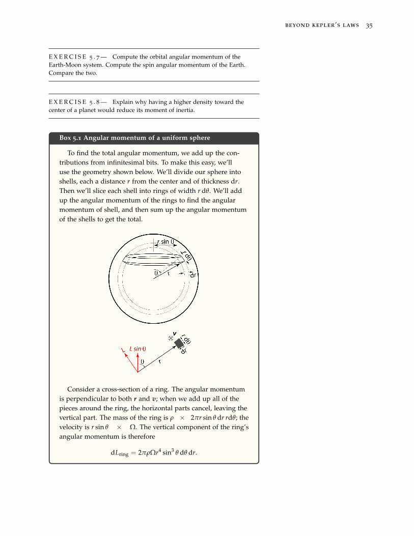
To find the total angular momentum, we add up the con-tributions from infinitesimal bits. To make this easy, we’lluse the geometry shown below. We’ll divide our sphere intoshells, each a distance r from the center and of thickness dr.Then we’ll slice each shell into rings of width r dθ. We’ll addup the angular momentum of the rings to find the angularmomentum of shell, and then sum up the angular momentumof the shells to get the total.
Consider a cross-section of a ring. The angular momentumis perpendicular to both r and v; when we add up all of thepieces around the ring, the horizontal parts cancel, leaving thevertical part. The mass of the ring is ρ × 2πr sin θ dr rdθ; thevelocity is r sin θ × Ω. The vertical component of the ring’sangular momentum is therefore
dLring = 2πρΩr4 sin3 θ dθ dr.
36 planets and telescopes
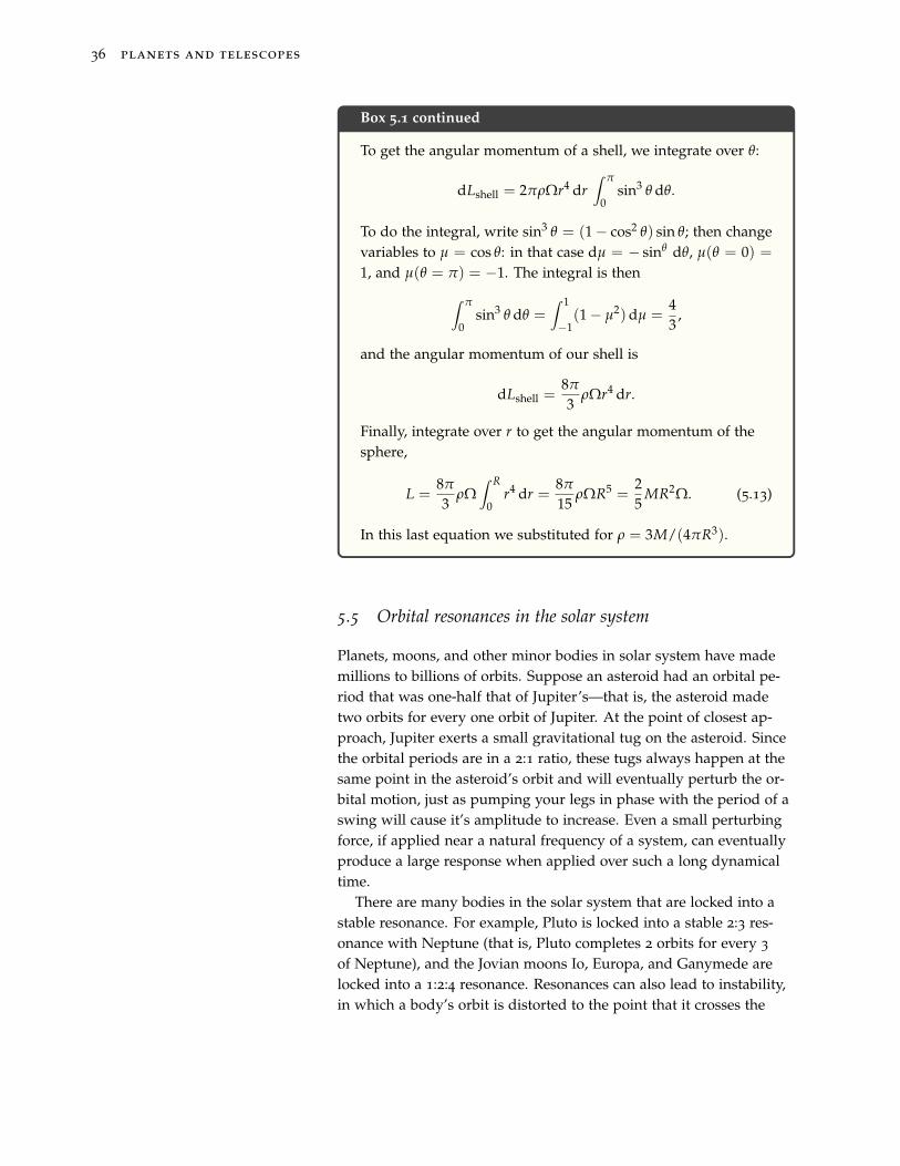
Box 5.1 continued
To get the angular momentum of a shell, we integrate over θ:
dLshell = 2πρΩr4 dr∫ π
0sin3 θ dθ.
To do the integral, write sin3 θ = (1− cos2 θ) sin θ; then changevariables to µ = cos θ: in that case dµ = − sinθ dθ, µ(θ = 0) =1, and µ(θ = π) = −1. The integral is then∫ π
0sin3 θ dθ =
∫ 1
−1(1− µ2)dµ =
43
,
and the angular momentum of our shell is
dLshell =8π
3ρΩr4 dr.
Finally, integrate over r to get the angular momentum of thesphere,
L =8π
3ρΩ
∫ R
0r4 dr =
8π
15ρΩR5 =
25
MR2Ω. (5.13)
In this last equation we substituted for ρ = 3M/(4πR3).
5.5 Orbital resonances in the solar system
Planets, moons, and other minor bodies in solar system have mademillions to billions of orbits. Suppose an asteroid had an orbital pe-riod that was one-half that of Jupiter’s—that is, the asteroid madetwo orbits for every one orbit of Jupiter. At the point of closest ap-proach, Jupiter exerts a small gravitational tug on the asteroid. Sincethe orbital periods are in a 2:1 ratio, these tugs always happen at thesame point in the asteroid’s orbit and will eventually perturb the or-bital motion, just as pumping your legs in phase with the period of aswing will cause it’s amplitude to increase. Even a small perturbingforce, if applied near a natural frequency of a system, can eventuallyproduce a large response when applied over such a long dynamicaltime.
There are many bodies in the solar system that are locked into astable resonance. For example, Pluto is locked into a stable 2:3 res-onance with Neptune (that is, Pluto completes 2 orbits for every 3
of Neptune), and the Jovian moons Io, Europa, and Ganymede arelocked into a 1:2:4 resonance. Resonances can also lead to instability,in which a body’s orbit is distorted to the point that it crosses the
beyond kepler’s laws 37
orbit of another planet, at which point that body either collides withthe other planet or is scattered out of the solar system. For example,the Kirkwood gap in the asteroid belt is located at the 3:1 resonancewith Jupiter (see Fig. 2.10 of Lissauer and de Pater5). Numerical cal- 5 Jack J. Lissauer and Imke de Pater.
Fundamental Planetary Science: Physics,Chemistry and Habitability. CambridgeUniversity Press, 2013
culations find that the precession of Mercury’s perihelion is cominginto resonance with that of Jupiter, leading to a 1% chance over thenext 5 Gyr of Mercury colliding with the Sun or Venus, and a smallerpossibility of the entire inner solar system becoming unstable6 over 6 J. Laskar and M. Gastineau. Existence
of collisional trajectories of Mercury,Mars and Venus with the Earth. Na-ture, 459:817–819, June 2009. doi:10.1038/nature08096
that time.
Torques exerted on a planet’s equatorial bulge by othersolar system bodies can cause that planet’s obliquity to vary. Saturn’slarge (relative to Jupiter) axial tilt is thought to be caused by a spin-orbit resonance between the precession of Saturn’s axis the precessionof Neptune’s orbital plane7. Mars’s axial tilt wanders considerably 7 W. R. Ward and D. P. Hamilton. Tilting
Saturn. I. Analytic Model. Astron.Journ., 128:2501–2509, November 2004.doi: 10.1086/424533
over a few Myr timescale and has reached tilts as large as 60 in thepast. The large moment of inertia of the Earth-Moon system keepsEarth’s axial tilt from wandering to such extreme values; neverthe-less, the Earth’s inclination does oscillate by < 1 on a 40 000 yrtimescale. This wandering of the inclination, along with variations inthe orbital eccentricity, are thought to explain the quasi-periodic iceages on Earth over the last few million years8. 8 J. Zachos, M. Pagani, L. Sloan,
E. Thomas, and K. Billups. Trends,Rhythms, and Aberrations in GlobalClimate 65 Ma to Present. Science, 292:686–693, April 2001. doi: 10.1126/sci-ence.1059412

6Planetary Atmospheres
It’s more important to know whether there will be weather than whatthe weather will be. —Norton Juster, The Phantom Tollbooth
6.1 Hydrostatic equilibrium
Let’s consider a fluid at rest in a gravitational field. By at rest, wesimply mean that the fluid velocity is sufficiently small that we canneglect the inertia of the moving fluid in our equation for force bal-ance. By a fluid, we mean that the pressure is isotropic1 and directed 1 Meaning the pressure is the same in
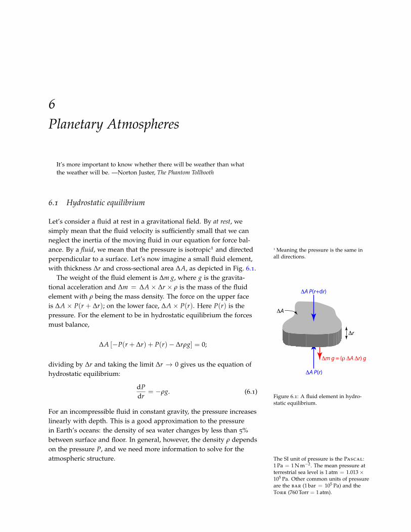
all directions.perpendicular to a surface. Let’s now imagine a small fluid element,with thickness ∆r and cross-sectional area ∆A, as depicted in Fig. 6.1.
ΔA
Δr
ΔA P(r+dr)
ΔA P(r)
Δm g = (ρ ΔA Δr) g
Figure 6.1: A fluid element in hydro-static equilibrium.
The weight of the fluid element is ∆m g, where g is the gravita-tional acceleration and ∆m = ∆A × ∆r × ρ is the mass of the fluidelement with ρ being the mass density. The force on the upper faceis ∆A × P(r + ∆r); on the lower face, ∆A × P(r). Here P(r) is thepressure. For the element to be in hydrostatic equilibrium the forcesmust balance,
∆A [−P(r + ∆r) + P(r)− ∆rρg] = 0;
dividing by ∆r and taking the limit ∆r → 0 gives us the equation ofhydrostatic equilibrium:
dPdr
= −ρg. (6.1)
For an incompressible fluid in constant gravity, the pressure increaseslinearly with depth. This is a good approximation to the pressurein Earth’s oceans: the density of sea water changes by less than 5%between surface and floor. In general, however, the density ρ dependson the pressure P, and we need more information to solve for theatmospheric structure. The SI unit of pressure is the Pascal:
1 Pa = 1 N m−2. The mean pressure atterrestrial sea level is 1 atm = 1.013×10⁵ Pa. Other common units of pressureare the bar (1 bar = 105 Pa) and theTorr (760 Torr = 1 atm).
40 planets and telescopes
E X E R C I S E 6 . 1 — Water is nearly incompressible and has a density of103 kg m−3. How deep would you need to dive for the pressure to increaseby 1 atm = 1.013× 10⁵ Pa? The gravitational acceleration at Earth’s surface is9.8 m s−2.
Let’s look at this in a bit more detail. Suppose we take our fluidlayer to be thin, so that g is approximately constant. Then we canwrite equation (6.1) as ∫ P(z)
P0
dP = −g∫ z
0ρ dz.
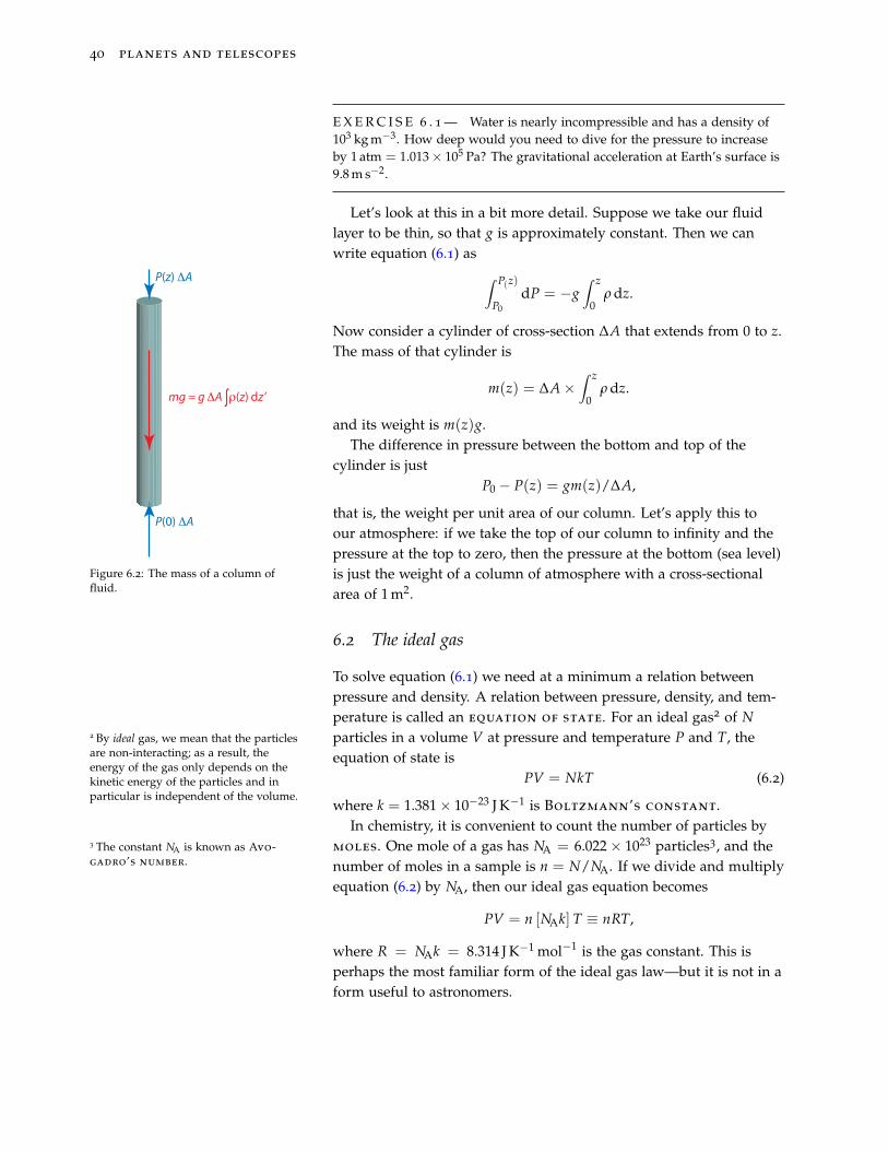
Now consider a cylinder of cross-section ∆A that extends from 0 to z.The mass of that cylinder is
m(z) = ∆A×∫ z
0ρ dz.
and its weight is m(z)g.
P(z) ΔA
P(0) ΔA
mg = g ΔA ∫ρ(z) dz’
Figure 6.2: The mass of a column offluid.
The difference in pressure between the bottom and top of thecylinder is just
P0 − P(z) = gm(z)/∆A,
that is, the weight per unit area of our column. Let’s apply this toour atmosphere: if we take the top of our column to infinity and thepressure at the top to zero, then the pressure at the bottom (sea level)is just the weight of a column of atmosphere with a cross-sectionalarea of 1 m2.
6.2 The ideal gas
To solve equation (6.1) we need at a minimum a relation betweenpressure and density. A relation between pressure, density, and tem-perature is called an equation of state. For an ideal gas2 of N
2 By ideal gas, we mean that the particlesare non-interacting; as a result, theenergy of the gas only depends on thekinetic energy of the particles and inparticular is independent of the volume.
particles in a volume V at pressure and temperature P and T, theequation of state is
PV = NkT (6.2)
where k = 1.381× 10⁻²³ J K−1 is Boltzmann’s constant.In chemistry, it is convenient to count the number of particles by
moles. One mole of a gas has NA = 6.022× 10²³ particles3, and the3 The constant NA is known as Avo-gadro’s number. number of moles in a sample is n = N/NA. If we divide and multiply
equation (6.2) by NA, then our ideal gas equation becomes
PV = n [NAk] T ≡ nRT,
where R = NAk = 8.314 J K−1 mol−1 is the gas constant. This isperhaps the most familiar form of the ideal gas law—but it is not in aform useful to astronomers.
planetary atmospheres 41
We astronomers don’t care about little beakers of fluid—we havewhole worlds to model! Let’s take our ideal gas law and introducethe molar weight m as the mass of one mole of our gas. Then theideal gas law can be written
P =
(mN/NA
V
)kNA
mT ≡ ρ
kNA
mT. (6.3)
The quantity in parenthesis is the mass per volume, or density ρ,of our fluid. This is the same mass density that appears in equa-tion (6.1). Equation (6.3) is the form most convenient for fluid dy-namics, because it is in terms of intrinsic fluid properties rather thanin terms of a laboratory quantity like volume.
6.3 The scale height
Let’s take a first stab at modeling Earth’s atmosphere with equa-tion (6.1). We’ll take Earth’s atmosphere to be an ideal gas and forsimplicity we’ll assume the temperature doesn’t change with al-titude4. The molar weight of dry5 air is 0.02897 kg mol−1. Using
4 This isn’t true, of course, but let’s keepthings simple and see how we do.
5 The water vapor content of air variesconsiderably depending on ambientconditions.
equation (6.3) to eliminate ρ in equation (6.1), we obtain
1P
dPdz
= − mgNAkT
, ordPP
= − mgNAkT
dz.
Integrating from z = 0, where P(z = 0) = P0, to a height z gives us anequation for the pressure as a function of height,
P(z) = P0 exp[− mgz
NAkT
]. (6.4)
Since the argument of the exponential is dimensionless, we see thatwe can write P(z) = P0e−z/HP , where
HP =NAkT
mg
is the pressure scale height—the height over which the pressuredecreases by a factor 1/e.
E X E R C I S E 6 . 2 — Evaluate HP for dry air at a temperature of 288 K(15 C). Check that your answer is reasonable based on your experience. Infact, this value of HP is overly large because the temperature in thetroposphere does, in fact, decrease with height at an average lapse rate of
dTdz
= −6.5 C km−1.
42 planets and telescopes
6.4 The adiabatic thermal gradient
Hot air rises. This simple phenomenon sets the lapse rate, dT/dz, inthe troposphere. Sunlight is absorbed by the land and water, whichwarms the overlying atmosphere. This warm surface then rises, whilecolder air sinks. This movement is sufficiently rapid that there is littleexchange of heat between the warm, rising air and the cool, sinkingair. As a result, the fluid motions are adiabatic. To understandwhat this means, recall the first law of thermodynamics6, which6 Enrico Fermi. Thermodynamics. Dover,
1956 relates the change in internal energy dU and in volume dV to theheat transferred dQ:
dQ = dU + PdV, (6.5)
where P is the pressure. During an adiabatic process, dQ = 0, andone can show that
PVγ = const.,
where γ = CP/CV is the ratio of specific heats (Table 6.1). Hence, if
Table 6.1: Specific heats for ideal gases. gas Cρ CP = Cρ + kNA/m γ = CP/Cρ
monatomic (3/2)kNA/m (5/2)kNA/m 5/3diatomic (5/2)kNA/m (7/2)kNA/m 7/5
the pressure and volume (of some specified mass of air) at the bottomof the atmosphere are P0 and V0, then the pressure and volume ofthat mass at elevation is given by
PVγ = const = P0Vγ.0
Now, let’s use the ideal gas law (eq. 6.2) to express V = NkT/P; for afixed N, this gives
P1−γTγ = P1−γ0 Tγ
0 ,
or
T = T0
(PP0
)(γ−1)/γ
. (6.6)
Equation (6.6) tells us how the temperature changes with pressurealong an adiabat for an ideal gas.
E X E R C I S E 6 . 3 — Use equations (6.6) and (6.1) to compute the lapserate dT/dz at sea level. Dry air is composed of mostly diatomic gases with amolar weight 0.02897 kg mol−1. You should find an answer around−10 C/km, which is almost twice as large as the value quoted earlier. Canyou guess why the value you calculated might be off? (Hint: there is a processwe haven’t yet accounted for. If you want a hint, go outside and look up.)
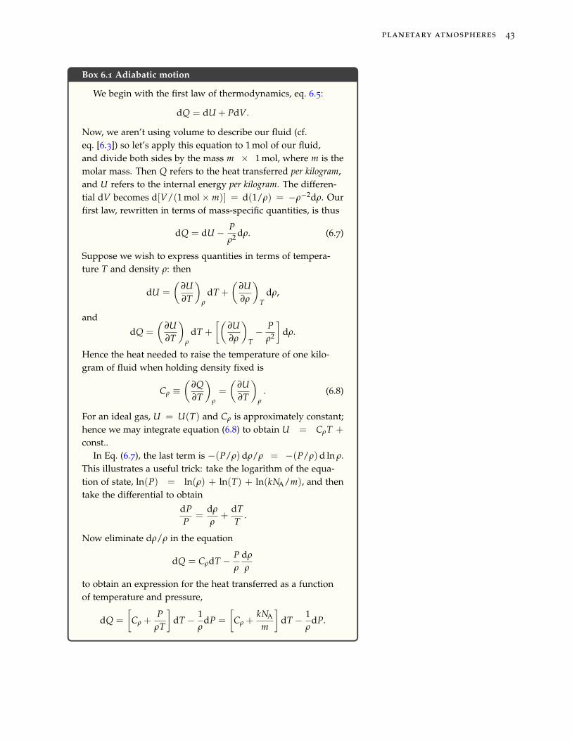
planetary atmospheres 43
Box 6.1 Adiabatic motion
We begin with the first law of thermodynamics, eq. 6.5:
dQ = dU + PdV.
Now, we aren’t using volume to describe our fluid (cf.eq. [6.3]) so let’s apply this equation to 1 mol of our fluid,and divide both sides by the mass m × 1 mol, where m is themolar mass. Then Q refers to the heat transferred per kilogram,and U refers to the internal energy per kilogram. The differen-tial dV becomes d[V/(1 mol × m)] = d(1/ρ) = −ρ−2dρ. Ourfirst law, rewritten in terms of mass-specific quantities, is thus
dQ = dU − Pρ2 dρ. (6.7)
Suppose we wish to express quantities in terms of tempera-ture T and density ρ: then
dU =
(∂U∂T
)ρ
dT +
(∂U∂ρ
)T
dρ,
and
dQ =
(∂U∂T
)ρ
dT +
[(∂U∂ρ
)T− P
ρ2
]dρ.
Hence the heat needed to raise the temperature of one kilo-gram of fluid when holding density fixed is
Cρ ≡(
∂Q∂T
)ρ
=
(∂U∂T
)ρ
. (6.8)
For an ideal gas, U = U(T) and Cρ is approximately constant;hence we may integrate equation (6.8) to obtain U = CρT +
const..In Eq. (6.7), the last term is −(P/ρ)dρ/ρ = −(P/ρ)d ln ρ.
This illustrates a useful trick: take the logarithm of the equa-tion of state, ln(P) = ln(ρ) + ln(T) + ln(kNA/m), and thentake the differential to obtain
dPP
=dρ
ρ+
dTT
.
Now eliminate dρ/ρ in the equation
dQ = CρdT − Pρ
dρ
ρ
to obtain an expression for the heat transferred as a functionof temperature and pressure,
dQ =
[Cρ +
PρT
]dT − 1
ρdP =
[Cρ +
kNA
m
]dT − 1
ρdP.
44 planets and telescopes
Box 6.1 continued
From this we see that the heat needed to raise the temperatureof one mole when holding pressure fixed is
CP ≡(
∂Q∂T
)P= CV +
kNA
m. (6.9)
The specific heat of one mole of various ideal gases is given inTable 6.1. It is important to remember that these relations forthe specific heats are for an ideal gas and are not universallytrue.
During convection, hot air rises and cool air de-scends, and both move adiabatically. By adiabatically,we mean that there is no heat exchange:
0 = dQ = CPdT − 1ρ
dP.
Using the ideal gas equation of state we can eliminate1ρ = (kNA/m)T/P and write
dTT
=kNA
mCP
dPP
=CP − CV
CP
dPP
=γ− 1
γ
dPP
.
Integrating both sides of the equation gives
ln T =γ− 1
γln P + const.,
which is equivalent to eq. (6.6).
6.5 Atmospheric circulation on a rotating Earth
The Sun heats the Earth unevenly; this in turn creates pressure gra-dients that drive a circulation of the atmosphere and a transfer forheat from the equator polewards. The Coriolis force deflects the hor-izontal motion of the air, and this sets up large-scale features in theatmosphere.
Because of the Earth’s rotation, in the frame of a particular locationon Earth there is both a Coriolis and a centrifugal acceleration:
Coriolis aCor = −2Ω× v (6.10)
centrifugal acen = −Ω× (Ω× R) (6.11)
where R is the location of our particle and Ω is the rotation vector ofthe Earth.
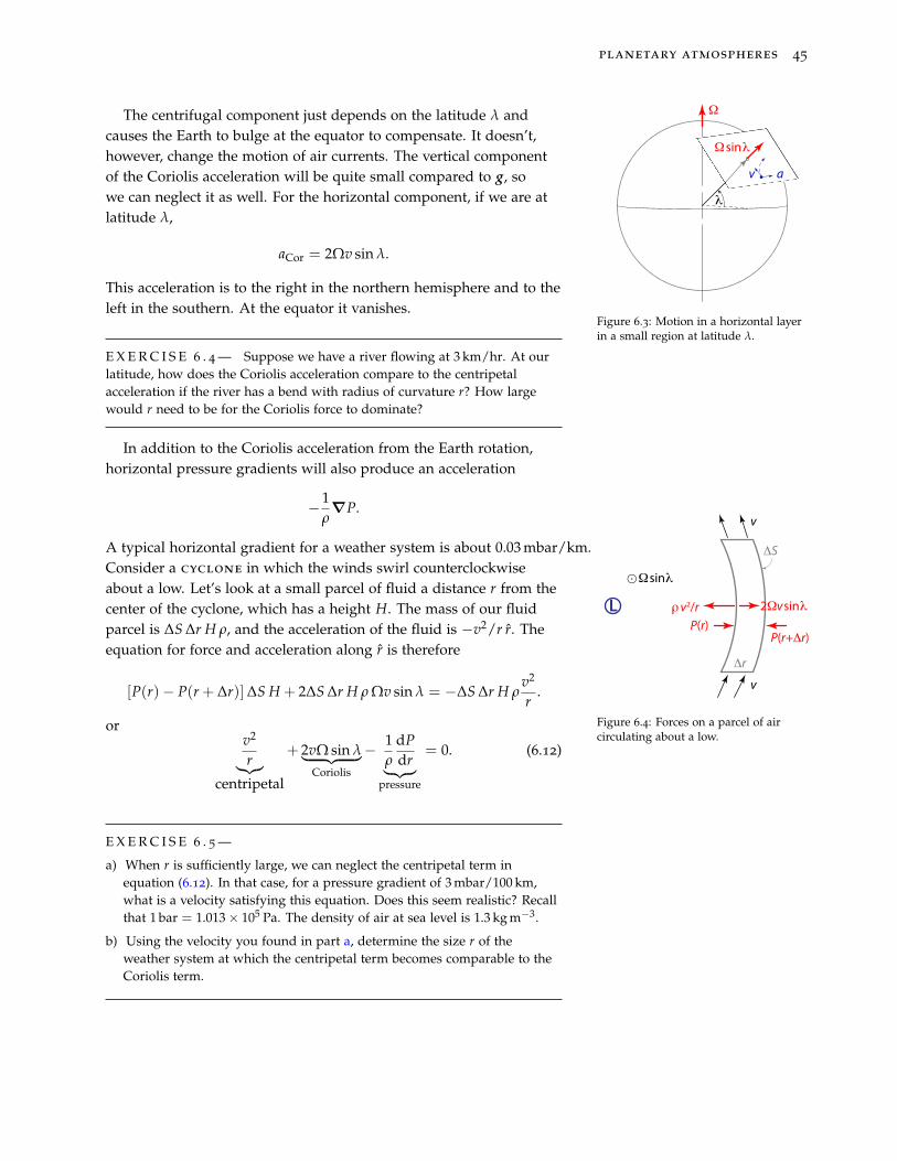
planetary atmospheres 45
The centrifugal component just depends on the latitude λ andcauses the Earth to bulge at the equator to compensate. It doesn’t,however, change the motion of air currents. The vertical componentof the Coriolis acceleration will be quite small compared to g, sowe can neglect it as well. For the horizontal component, if we are atlatitude λ,
λ
Ω
Ωsinλ
v a
Figure 6.3: Motion in a horizontal layerin a small region at latitude λ.
aCor = 2Ωv sin λ.
This acceleration is to the right in the northern hemisphere and to theleft in the southern. At the equator it vanishes.
E X E R C I S E 6 . 4 — Suppose we have a river flowing at 3 km/hr. At ourlatitude, how does the Coriolis acceleration compare to the centripetalacceleration if the river has a bend with radius of curvature r? How largewould r need to be for the Coriolis force to dominate?
In addition to the Coriolis acceleration from the Earth rotation,horizontal pressure gradients will also produce an acceleration
−1ρ∇P.
A typical horizontal gradient for a weather system is about 0.03 mbar/km.Consider a cyclone in which the winds swirl counterclockwiseabout a low. Let’s look at a small parcel of fluid a distance r from thecenter of the cyclone, which has a height H. The mass of our fluidparcel is ∆S ∆r H ρ, and the acceleration of the fluid is −v2/r r. Theequation for force and acceleration along r is therefore
L
P(r+Δr)
ρv2/rP(r)
v
v
Δr
ΔS
Ωsinλ
2Ωvsinλ
Figure 6.4: Forces on a parcel of aircirculating about a low.
[P(r)− P(r + ∆r)]∆S H + 2∆S ∆r H ρ Ωv sin λ = −∆S ∆r H ρv2
r.
orv2
r︸︷︷︸centripetal
+ 2vΩ sin λ︸ ︷︷ ︸Coriolis
− 1ρ
dPdr︸ ︷︷ ︸
pressure
= 0. (6.12)
E X E R C I S E 6 . 5 —
a) When r is sufficiently large, we can neglect the centripetal term inequation (6.12). In that case, for a pressure gradient of 3 mbar/100 km,what is a velocity satisfying this equation. Does this seem realistic? Recallthat 1 bar = 1.013× 10⁵ Pa. The density of air at sea level is 1.3 kg m−3.
b) Using the velocity you found in part a, determine the size r of theweather system at which the centripetal term becomes comparable to theCoriolis term.
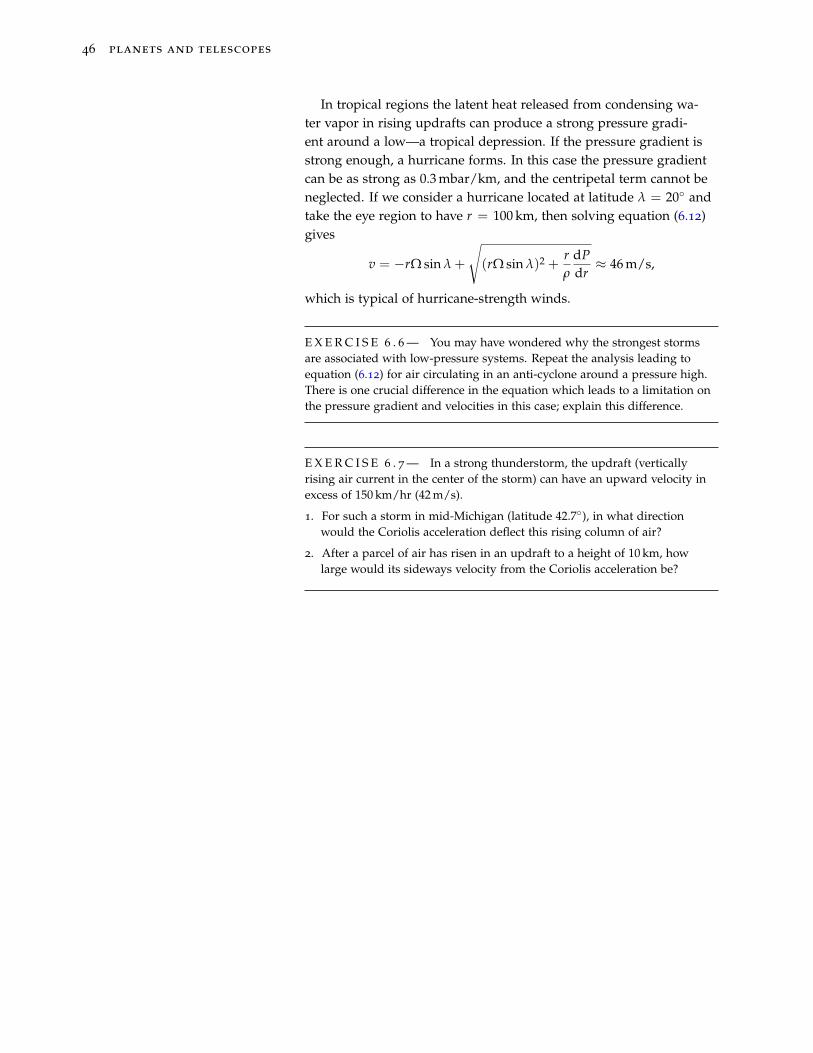
46 planets and telescopes
In tropical regions the latent heat released from condensing wa-ter vapor in rising updrafts can produce a strong pressure gradi-ent around a low—a tropical depression. If the pressure gradient isstrong enough, a hurricane forms. In this case the pressure gradientcan be as strong as 0.3 mbar/km, and the centripetal term cannot beneglected. If we consider a hurricane located at latitude λ = 20 andtake the eye region to have r = 100 km, then solving equation (6.12)gives
v = −rΩ sin λ +
√(rΩ sin λ)2 +
rρ
dPdr≈ 46 m/s,
which is typical of hurricane-strength winds.
E X E R C I S E 6 . 6 — You may have wondered why the strongest stormsare associated with low-pressure systems. Repeat the analysis leading toequation (6.12) for air circulating in an anti-cyclone around a pressure high.There is one crucial difference in the equation which leads to a limitation onthe pressure gradient and velocities in this case; explain this difference.
E X E R C I S E 6 . 7 — In a strong thunderstorm, the updraft (verticallyrising air current in the center of the storm) can have an upward velocity inexcess of 150 km/hr (42 m/s).
1. For such a storm in mid-Michigan (latitude 42.7), in what directionwould the Coriolis acceleration deflect this rising column of air?
2. After a parcel of air has risen in an updraft to a height of 10 km, howlarge would its sideways velocity from the Coriolis acceleration be?
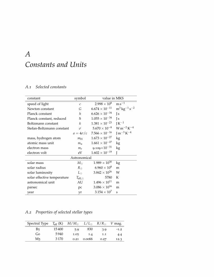
AConstants and Units
A.1 Selected constants
constant symbol value in MKS
speed of light c 2.998× 10⁸ m s−1
Newton constant G 6.674× 10⁻¹¹ m3 kg−1 s−2
Planck constant h 6.626× 10⁻³⁴ J sPlanck constant, reduced h 1.055× 10⁻³⁴ J sBoltzmann constant k 1.381× 10⁻²³ J K−1
Stefan-Boltzmann constant σ 5.670× 10⁻⁸ W m−2 K−4
a = 4σ/c 7.566× 10⁻¹⁶ J m−3 K−4
mass, hydrogen atom mH 1.673× 10⁻²⁷ kgatomic mass unit mu 1.661× 10⁻²⁷ kgelectron mass me 9.109×10⁻³¹ kgelectron volt eV 1.602× 10⁻¹⁹ J
Astronomicalsolar mass M 1.989× 1030 kgsolar radius R 6.960× 10⁸ msolar luminosity L 3.842× 1026 Wsolar effective temperature Teff, 5780 Kastronomical unit AU 1.496× 10¹¹ mparsec pc 3.086× 10¹⁶ myear yr 3.154× 10⁷ s
A.2 Properties of selected stellar types
Spectral Type Teff (K) M/M L/L R/R V mag.
B5 15 400 5.9 830 3.9 -1.2G0 5 940 1.05 1.4 1.1 4.4M5 3 170 0.21 0.0066 0.27 12.3
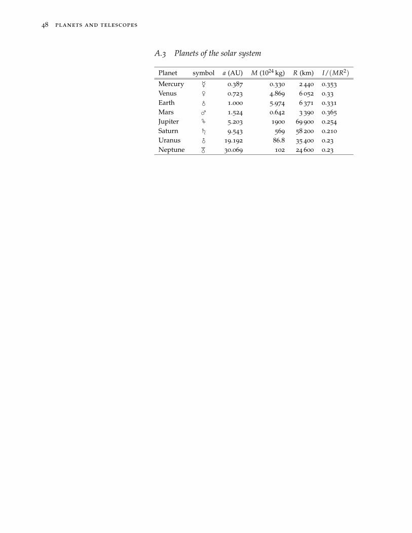
48 planets and telescopes
A.3 Planets of the solar system
Planet symbol a (AU) M (1024 kg) R (km) I/(MR2)
Mercury ' 0.387 0.330 2 440 0.353
Venus 0.723 4.869 6 052 0.33
Earth 1.000 5.974 6 371 0.331
Mars 1.524 0.642 3 390 0.365
Jupiter X 5.203 1900 69 900 0.254
Saturn Y 9.543 569 58 200 0.210
Uranus Z 19.192 86.8 35 400 0.23
Neptune [ 30.069 102 24 600 0.23
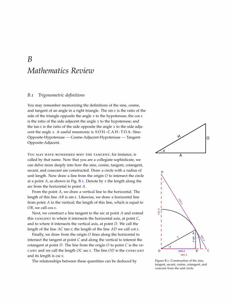
BMathematics Review
B.1 Trigonometric definitions
You may remember memorizing the definitions of the sine, cosine,and tangent of an angle in a right triangle. The sin x is the ratio of theside of the triangle opposite the angle x to the hypotenuse; the cos xis the ratio of the side adjacent the angle x to the hypotenuse; andthe tan x is the ratio of the side opposite the angle x to the side adja-cent the angle x. A useful mnemonic is S O H - C A H - T O A: Sine-Opposite-Hypotenuse — Cosine-Adjacent-Hypotenuse — Tangent-Opposite-Adjacent.
x
O
A
H
You may have wondered why the tangent, for instance, iscalled by that name. Now that you are a collegiate sophisticate, wecan delve more deeply into how the sine, cosine, tangent, cotangent,secant, and cosecant are constructed. Draw a circle with a radius ofunit length. Now draw a line from the origin O to intersect the circleat a point A, as shown in Fig. B.1. Denote by x the length along thearc from the horizontal to point A.
From the point A, we draw a vertical line to the horizontal. Thelength of this line AB is sin x. Likewise, we draw a horizontal linefrom point A to the vertical; the length of this line, which is equal toOB, we call cos x.
Next, we construct a line tangent to the arc at point A and extendthis tangent to where it intersects the horizontal axis, at point C,and to where it intersects the vertical axis, at point D. We call thelength of the line AC tan x; the length of the line AD we call cot x.
1
D
Ox
B C
A
cos x
cot x
tan x
csc x
sec x
sin x
Figure B.1: Construction of the sine,tangent, secant, cosine, cotangent, andcosecant from the unit circle.
Finally, we draw from the origin O lines along the horizontal tointersect the tangent at point C and along the vertical to interest thecotangent at point D. The line from the origin O to point C is the se-cant and we call the length OC sec x. The line OD is the cosecant
and its length is csc x.The relationships between these quantities can be deduced by
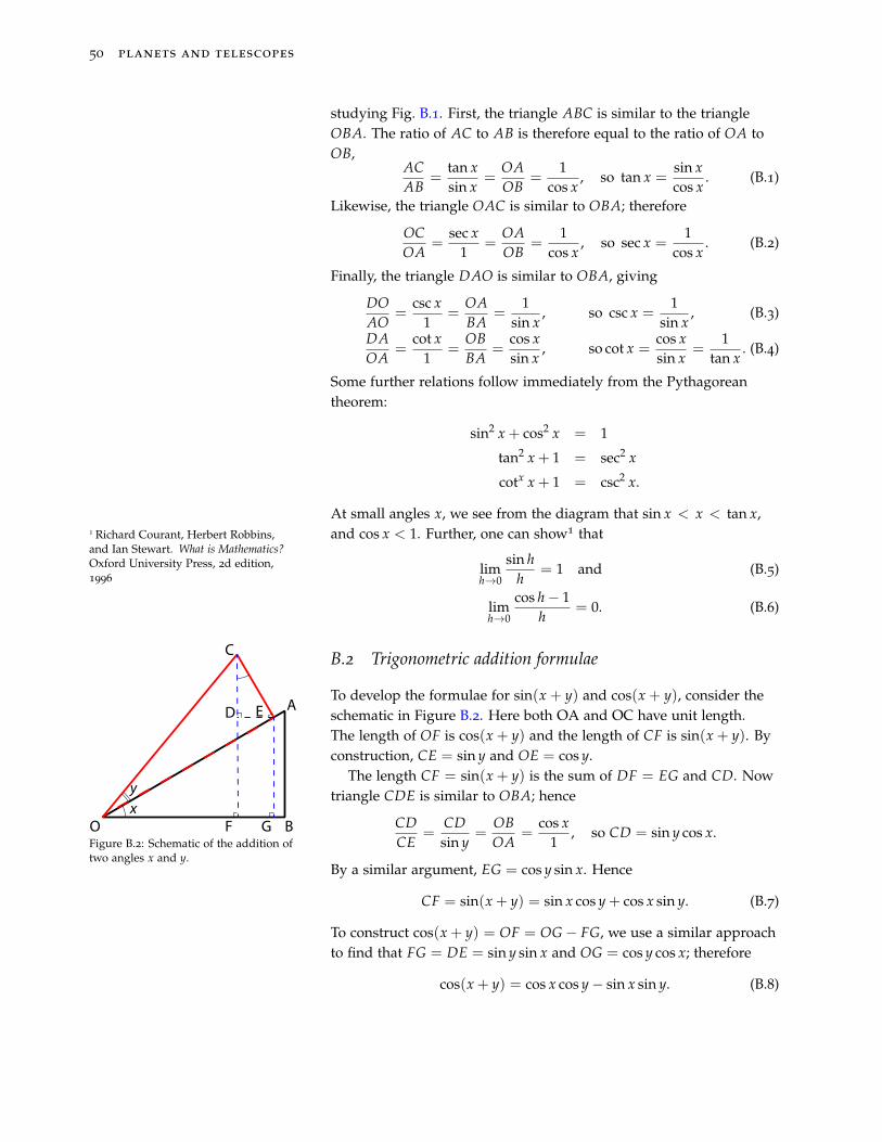
50 planets and telescopes
studying Fig. B.1. First, the triangle ABC is similar to the triangleOBA. The ratio of AC to AB is therefore equal to the ratio of OA toOB,
ACAB
=tan xsin x
=OAOB
=1
cos x, so tan x =
sin xcos x
. (B.1)
Likewise, the triangle OAC is similar to OBA; therefore
OCOA
=sec x
1=
OAOB
=1
cos x, so sec x =
1cos x
. (B.2)
Finally, the triangle DAO is similar to OBA, giving
DOAO
=csc x
1=
OABA
=1
sin x, so csc x =
1sin x
, (B.3)
DAOA
=cot x
1=
OBBA
=cos xsin x
, so cot x =cos xsin x
=1
tan x. (B.4)
Some further relations follow immediately from the Pythagoreantheorem:
sin2 x + cos2 x = 1
tan2 x + 1 = sec2 x
cotx x + 1 = csc2 x.
At small angles x, we see from the diagram that sin x < x < tan x,and cos x < 1. Further, one can show1 that1 Richard Courant, Herbert Robbins,
and Ian Stewart. What is Mathematics?Oxford University Press, 2d edition,1996
limh→0
sin hh
= 1 and (B.5)
limh→0
cos h− 1h
= 0. (B.6)
B.2 Trigonometric addition formulae
To develop the formulae for sin(x + y) and cos(x + y), consider theschematic in Figure B.2. Here both OA and OC have unit length.The length of OF is cos(x + y) and the length of CF is sin(x + y). Byconstruction, CE = sin y and OE = cos y.
xy
O
A
C
D E
F G BFigure B.2: Schematic of the addition oftwo angles x and y.
The length CF = sin(x + y) is the sum of DF = EG and CD. Nowtriangle CDE is similar to OBA; hence
CDCE
=CDsin y
=OBOA
=cos x
1, so CD = sin y cos x.
By a similar argument, EG = cos y sin x. Hence
CF = sin(x + y) = sin x cos y + cos x sin y. (B.7)
To construct cos(x + y) = OF = OG− FG, we use a similar approachto find that FG = DE = sin y sin x and OG = cos y cos x; therefore
cos(x + y) = cos x cos y− sin x sin y. (B.8)
mathematics review 51
B.3 Trigonometric derivatives
We can now use equations (B.5), (B.6), (B.7), and (B.8) to establishformulae for the derivatives of the sine and cosine. For the sine,using limh→0 sin h/h = 1 and limh→0(cos h− 1)/h = 0,
d sin xdx
= limh→0
sin(x + h)− sin xh
= limh→0
sin x cos h + cos x sin h− sin xh
= limh→0
(cos x
sin hh
+ sin xcos h− 1
h
)= cos x. (B.9)
Likewise,
d cos xdx
= limh→0
cos(x + h)− cos xh
= limh→0
cos x cos h− sin x sin h− cos xh
= − sin x. (B.10)
The formulae for the derivatives of the tangent, cotangent, secant,and cosecant can be derived by using the chain rule on equations (B.1)–(B.4).
B.4 The Taylor Expansion
Suppose we wish to approximate a function f (x) in the neighbor-hood of some point x0 by a power series. That it, we wish to write forsome h 1,
f (x = x0 + h) = c0 + c1h + c2h2 + c3h3 + c4h4 + . . .
We assume that f (x) is differentiable, and all those derivativesexist—no discontinuities or places where the derivative blows up.To find the constants c0, c1, c2, c3, . . ., we first set h = 0 and obtain
f (x0) = c0,
which fixes the first constant. Next, we take the derivative and seth = 0, x = x0
d f (x)dx
∣∣∣∣x=x0
=[c1 + 2c2h + 3c3h2 + 4c4h3 . . .
]h=0
= c1.
For the next term, we take another derivative,
d2 f (x)dx2
∣∣∣∣x=x0
=[2c2 + 3 · 2c3h + 4 · 3c4h2 . . .
]h=0
= 2c2.
52 planets and telescopes
Thus our expansion out to the term in h2 is
f (x0 + h) = f (x0) +d f (x)
dx
∣∣∣∣x=x0
h +12
d2 f (x)dx2
∣∣∣∣x=x0
h2 +O(h3).
Here the expressions O(h3) means that the remaining terms are ofthe same size as h3.
Applying this expansion to sin x and cos x about the point x0 = 0,we have to order h2,
sin h = sin(0) + cos(0)h− 12
sin(0)h2 + . . . ≈ h, (B.11)
cos h = cos(0)− sin(0)h− 12
cos(0)h2 + . . . ≈ 1− h2
2(B.12)
since sin(0) = 0, cos(0) = 1.
CProbability and Statistics
The true logic of this world is in the calculus of probabilities. —JamesClerk Maxwell
Astronomical observations produce data—sets of numbersfrom measurements. To advance our understanding of astronomy,we must compare this data to an underlying hypothesis or model. Tomake this comparison, we compute some statistic s from the dataD and assess the likelihood of the value of s given our hypothesis.
As a naive example, we might sum over the differences betweenthe predictions P = pi of a model and the observations Di:
s = ∑i(pi − Di)
2 .
The data Di could be the transit times for an exoplanet, and pi wouldbe our predicted transit times given a model of the orbit. In this case,s = 0 would signify perfect agreement. Nothing is ever perfect,however; what would we make of s being small but non-zero? Weneed a figure-of-merit1: given some small value of s, is it likely that 1 And of course, we want to find the
best choice of statistic s for assessinghow well the model fits the data.
the model is consistent with the data? If we judge the value of s to beimplausible, we say that the model, or hypothesis, is not supportedby the data.
The converse case of s having a value with a high probabilitydoes not, however, “rule in” the hypothesis—at best, the hypothesisis consistent with observations, but other hypotheses may also beconsistent. The goal is to amass an ever larger body of evidencesupporting the hypothesis, but one can never prove it conclusively.
C.1 Basic Rules of Probability and Combinatorics
Having motivated the problem, we now step back and ask, what ismeant by probability? We are familiar with many examples from oureveryday experience. What is the probability of drawing an ace from
54 planets and telescopes
a deck of cards? What is the probability of rain tomorrow? What isthe probability that our candidate will win the election?
E X E R C I S E C . 1 — Think of some different situations in which youmight use the word “probability”. How does the definition of probabilitydiffer among these situations?
It is not immediately obvious that different usages of the term areconsistent. To give two examples:
1. A “fair” die is cast; we say that the probability of rolling a • isP(•) = 1/6. What does this mean? We may mean that if wewere to roll the die a very large number of times N, or roll a largenumber N of dice, then the number of those tries yielding a •tends toward22 This definition carries the prior as-
sumption that all sides are equallylikely and that 0 ≤ P ≤ 1. P(•) = lim
N→∞
N(•)N
=16
.
Note that this is an assertion: if we did this experiment and foundthat Pexp(•) 6= 1/6, we would claim the die is loaded!
2. The Newtonian constant of gravitation is
G = (6.67384± 80)× 10−11 m3 kg−1 s−2.
What does the “±80” mean? It signifies that the value of G hassome specified probability of lying in the interval 6.67304 ≤ G ×1011 ≤ 6.67464. This is a different sense of probability than that inthe first example: the value of G has a single, definite value, andhere the probability reflects the degree of certainty we attach to itsmeasured value.
To start making this more precise, let’s introduce some terms3:3 Richard Durrett. The Essentials ofProbability. Duxbury Press, Belmont,CA, 1994
For an experiment or observation there is a set of all possible out-comes, called the sample space. A subset of possible outcomes isan event. We describe our events as subsets of a sample space Ω,as shown in Figure C.1. We write, e.g., A ⊂ Ω. An impossible eventis ∅, the empty set. When we say “not A” we mean Ac, the comple-ment of A (shaded region in Fig. C.2). When we say “A or B” wemean “A or B or both” and denote this by A ∪ B (Fig. C.3). Finally,when we say “A and B” we write A ∩ B (Fig. C.4). If “A and B aremutually exclusive” then we write A ∩ B = ∅ and we say that thesets are disjoint, like A and B in Fig. C.1.
For example, if we roll two dice, there are 6× 6 = 36 possible out-comes. This is our sample space. Suppose we wish to have the sumof our two dice be seven; we’ll call this event A. There are six suchpossibilities for event A: (1, 6), (2, 5), (3, 4), (4, 3), (5, 2), (6, 1). Now
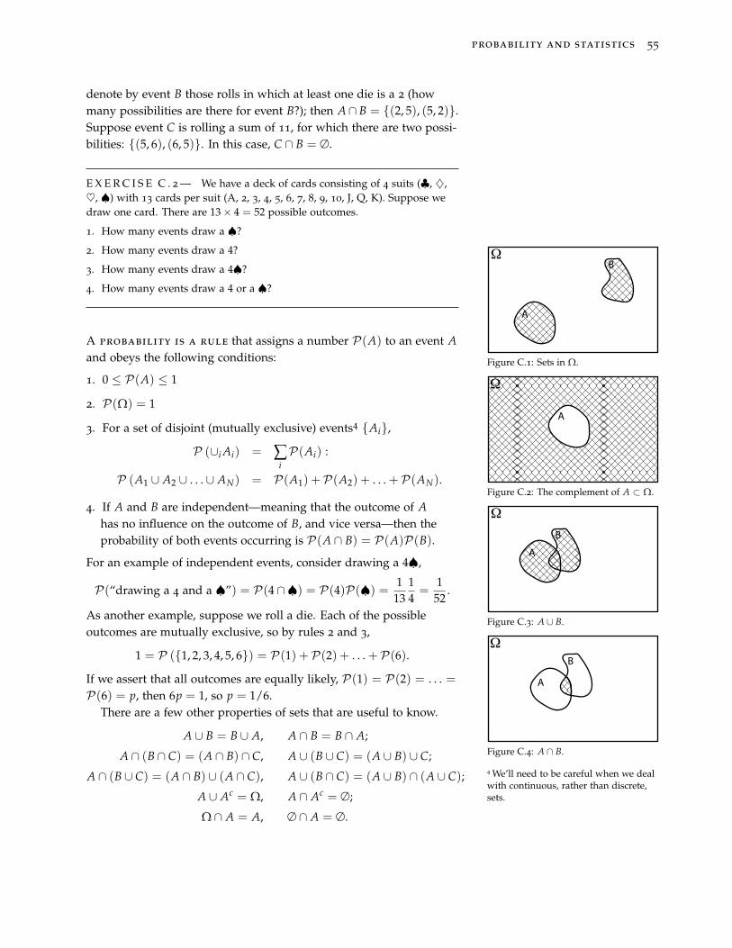
probability and statistics 55
denote by event B those rolls in which at least one die is a 2 (howmany possibilities are there for event B?); then A∩ B = (2, 5), (5, 2).Suppose event C is rolling a sum of 11, for which there are two possi-bilities: (5, 6), (6, 5). In this case, C ∩ B = ∅.
E X E R C I S E C . 2 — We have a deck of cards consisting of 4 suits (♣, ♦,♥, ♠) with 13 cards per suit (A, 2, 3, 4, 5, 6, 7, 8, 9, 10, J, Q, K). Suppose wedraw one card. There are 13× 4 = 52 possible outcomes.
1. How many events draw a ♠?
2. How many events draw a 4?
3. How many events draw a 4♠?
4. How many events draw a 4 or a ♠?
ΩB
A
Figure C.1: Sets in Ω.
Ω
A
Figure C.2: The complement of A ⊂ Ω.
Ω
B
A
Figure C.3: A ∪ B.
Ω
A
B
Figure C.4: A ∩ B.
A probability is a rule that assigns a number P(A) to an event Aand obeys the following conditions:
1. 0 ≤ P(A) ≤ 1
2. P(Ω) = 1
3. For a set of disjoint (mutually exclusive) events4 Ai,
4 We’ll need to be careful when we dealwith continuous, rather than discrete,sets.
P (∪i Ai) = ∑iP(Ai) :
P (A1 ∪ A2 ∪ . . . ∪ AN) = P(A1) + P(A2) + . . . + P(AN).
4. If A and B are independent—meaning that the outcome of Ahas no influence on the outcome of B, and vice versa—then theprobability of both events occurring is P(A ∩ B) = P(A)P(B).
For an example of independent events, consider drawing a 4♠,
P(“drawing a 4 and a ♠”) = P(4∩♠) = P(4)P(♠) = 113
14=
152
.
As another example, suppose we roll a die. Each of the possibleoutcomes are mutually exclusive, so by rules 2 and 3,
1 = P (1, 2, 3, 4, 5, 6) = P(1) + P(2) + . . . + P(6).
If we assert that all outcomes are equally likely, P(1) = P(2) = . . . =P(6) = p, then 6p = 1, so p = 1/6.
There are a few other properties of sets that are useful to know.
A ∪ B = B ∪ A, A ∩ B = B ∩ A;
A ∩ (B ∩ C) = (A ∩ B) ∩ C, A ∪ (B ∪ C) = (A ∪ B) ∪ C;
A ∩ (B ∪ C) = (A ∩ B) ∪ (A ∩ C), A ∪ (B ∩ C) = (A ∪ B) ∩ (A ∪ C);
A ∪ Ac = Ω, A ∩ Ac = ∅;
Ω ∩ A = A, ∅ ∩ A = ∅.
56 planets and telescopes
Using these properties and our rules for assigning probabilities,we can deduce a few more formulae. For example, P(Ac ∪ A) =
P(Ac) + P(A) = P(Ω) = 1; therefore, P(Ac) = 1−P(A). Likewise,we can show that P(∅) = 0. Finally, we can show that if A and B arenot mutually exclusive, but have some overlap, then
P(A ∪ B) = P(A) + P(B)−P(A ∩ B).
We encountered an instance of this last rule in exercise C.2: P(4 ∪♠) = P(4) + P(♠)−P(4∩♠).
E X E R C I S E C . 3 — Suppose we draw 1 card from each of 2 decks. Findthe probability that at least one card is an ace, using the following twoformulae:
P(“from deck 1 or from deck 2”) = P(“from deck 1”) + P(“from deck 2”)
−P(“from both deck 1 and deck 2”).
P(“at least one ace”) = 1−P(“drawing no ace”).
We next need to consider different arrangements of items
in a set. For example, suppose we want to put 5 people in a line.How many ways are there to do this? For the first spot there are 5
choices. After assigning this first spot, we move to the second forwhich there are now 4 choices. Proceeding along in this fashion, thenumber of possible arrangements is 5 · 4 · 3 · 2 · 1 ≡ 5!.The factorial fcn. is recursively defined
by m! = m · (m− 1)!, with 0! = 1, 1! = 1. Suppose we are not picking everything in our set; for example, in aclass of 32 we may wish to select just 3 people for different jobs. Thenumber of possibilities is
P(32, 3) = 32 · 31 · 30 =32 · 31 · 30 · 29 · . . . · 1
29 · . . . 1=
32!(32− 3)!
. (C.1)
Here P(n, k) means we are picking k items from a set of n items.Now suppose we aren’t picking individuals for distinct jobs,
but just 3 individuals. In this case, the order of how we pick isirrelevant—Autumn, Brook, and Collin is the same as Brook, Collin,and Autumn. To avoid over-counting different arrangements, wedivide P(32, 3) from equation (C.1) by 3!, giving
“32 choose 3” ≡(
323
)≡ C32
3 =32!
(32− 3)!3!. (C.2)
More formally, (nm) is the number of ways of choosing m objects from
a set of n, without regard to order.One example you may have seen often is the expansion of a bino-
mial. For example, suppose we wish to expand (a + b)5. There are a
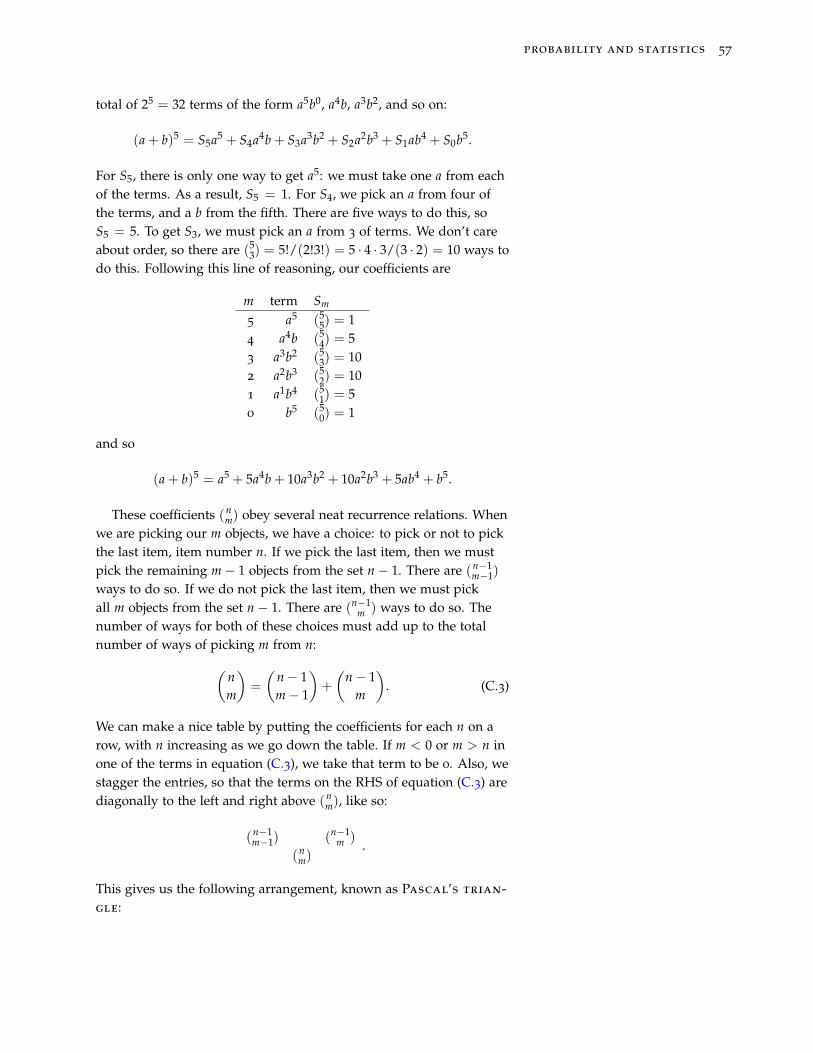
probability and statistics 57
total of 25 = 32 terms of the form a5b0, a4b, a3b2, and so on:
(a + b)5 = S5a5 + S4a4b + S3a3b2 + S2a2b3 + S1ab4 + S0b5.
For S5, there is only one way to get a5: we must take one a from eachof the terms. As a result, S5 = 1. For S4, we pick an a from four ofthe terms, and a b from the fifth. There are five ways to do this, soS5 = 5. To get S3, we must pick an a from 3 of terms. We don’t careabout order, so there are (5
3) = 5!/(2!3!) = 5 · 4 · 3/(3 · 2) = 10 ways todo this. Following this line of reasoning, our coefficients are
m term Sm
5 a5 (55) = 1
4 a4b (54) = 5
3 a3b2 (53) = 10
2 a2b3 (52) = 10
1 a1b4 (51) = 5
0 b5 (50) = 1
and so
(a + b)5 = a5 + 5a4b + 10a3b2 + 10a2b3 + 5ab4 + b5.
These coefficients (nm) obey several neat recurrence relations. When
we are picking our m objects, we have a choice: to pick or not to pickthe last item, item number n. If we pick the last item, then we mustpick the remaining m− 1 objects from the set n− 1. There are (n−1
m−1)
ways to do so. If we do not pick the last item, then we must pickall m objects from the set n − 1. There are (n−1
m ) ways to do so. Thenumber of ways for both of these choices must add up to the totalnumber of ways of picking m from n:(
nm
)=
(n− 1m− 1
)+
(n− 1
m
). (C.3)
We can make a nice table by putting the coefficients for each n on arow, with n increasing as we go down the table. If m < 0 or m > n inone of the terms in equation (C.3), we take that term to be 0. Also, westagger the entries, so that the terms on the RHS of equation (C.3) arediagonally to the left and right above (n
m), like so:
(n−1m−1) (n−1
m )
(nm)
.
This gives us the following arrangement, known as Pascal’s trian-gle:
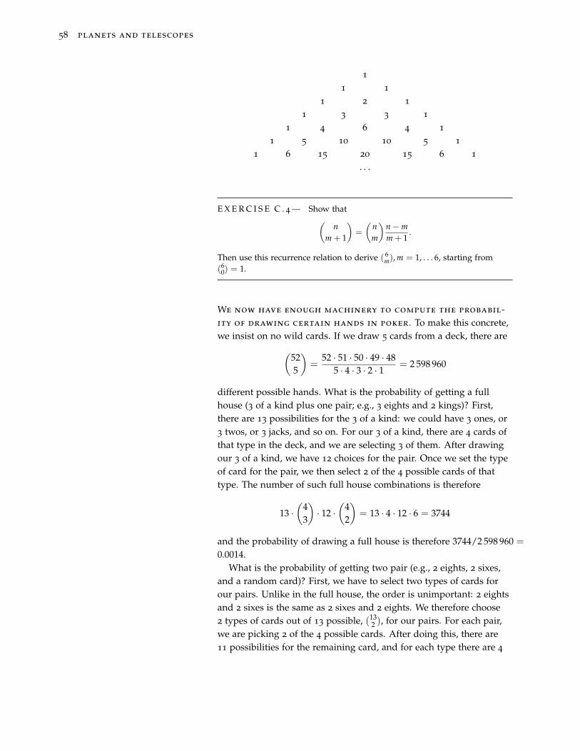
58 planets and telescopes
1
1 1
1 2 1
1 3 3 1
1 4 6 4 1
1 5 10 10 5 1
1 6 15 20 15 6 1
. . .
E X E R C I S E C . 4 — Show that(n
m + 1
)=
(nm
)n−mm + 1
.
Then use this recurrence relation to derive ( 6m), m = 1, . . . 6, starting from
(60) = 1.
We now have enough machinery to compute the probabil-ity of drawing certain hands in poker. To make this concrete,we insist on no wild cards. If we draw 5 cards from a deck, there are(
525
)=
52 · 51 · 50 · 49 · 485 · 4 · 3 · 2 · 1 = 2 598 960
different possible hands. What is the probability of getting a fullhouse (3 of a kind plus one pair; e.g., 3 eights and 2 kings)? First,there are 13 possibilities for the 3 of a kind: we could have 3 ones, or3 twos, or 3 jacks, and so on. For our 3 of a kind, there are 4 cards ofthat type in the deck, and we are selecting 3 of them. After drawingour 3 of a kind, we have 12 choices for the pair. Once we set the typeof card for the pair, we then select 2 of the 4 possible cards of thattype. The number of such full house combinations is therefore
13 ·(
43
)· 12 ·
(42
)= 13 · 4 · 12 · 6 = 3744
and the probability of drawing a full house is therefore 3744/2 598 960 =
0.0014.What is the probability of getting two pair (e.g., 2 eights, 2 sixes,
and a random card)? First, we have to select two types of cards forour pairs. Unlike in the full house, the order is unimportant: 2 eightsand 2 sixes is the same as 2 sixes and 2 eights. We therefore choose2 types of cards out of 13 possible, (13
2 ), for our pairs. For each pair,we are picking 2 of the 4 possible cards. After doing this, there are11 possibilities for the remaining card, and for each type there are 4
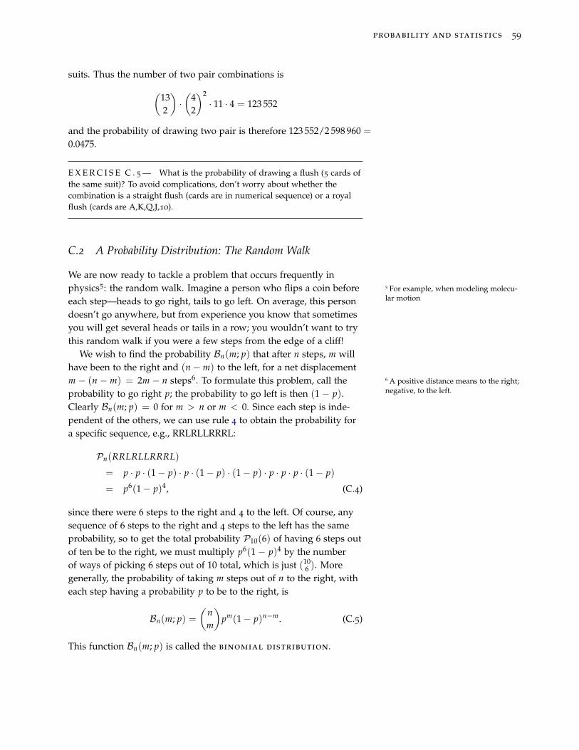
probability and statistics 59
suits. Thus the number of two pair combinations is(132
)·(
42
)2· 11 · 4 = 123 552
and the probability of drawing two pair is therefore 123 552/2 598 960 =
0.0475.
E X E R C I S E C . 5 — What is the probability of drawing a flush (5 cards ofthe same suit)? To avoid complications, don’t worry about whether thecombination is a straight flush (cards are in numerical sequence) or a royalflush (cards are A,K,Q,J,10).
C.2 A Probability Distribution: The Random Walk
We are now ready to tackle a problem that occurs frequently inphysics5: the random walk. Imagine a person who flips a coin before 5 For example, when modeling molecu-
lar motioneach step—heads to go right, tails to go left. On average, this persondoesn’t go anywhere, but from experience you know that sometimesyou will get several heads or tails in a row; you wouldn’t want to trythis random walk if you were a few steps from the edge of a cliff!
We wish to find the probability Bn(m; p) that after n steps, m willhave been to the right and (n−m) to the left, for a net displacementm − (n − m) = 2m − n steps6. To formulate this problem, call the 6 A positive distance means to the right;
negative, to the left.probability to go right p; the probability to go left is then (1 − p).Clearly Bn(m; p) = 0 for m > n or m < 0. Since each step is inde-pendent of the others, we can use rule 4 to obtain the probability fora specific sequence, e.g., RRLRLLRRRL:
Pn(RRLRLLRRRL)
= p · p · (1− p) · p · (1− p) · (1− p) · p · p · p · (1− p)
= p6(1− p)4, (C.4)
since there were 6 steps to the right and 4 to the left. Of course, anysequence of 6 steps to the right and 4 steps to the left has the sameprobability, so to get the total probability P10(6) of having 6 steps outof ten be to the right, we must multiply p6(1− p)4 by the numberof ways of picking 6 steps out of 10 total, which is just (10
6 ). Moregenerally, the probability of taking m steps out of n to the right, witheach step having a probability p to be to the right, is
Bn(m; p) =(
nm
)pm(1− p)n−m. (C.5)
This function Bn(m; p) is called the binomial distribution.
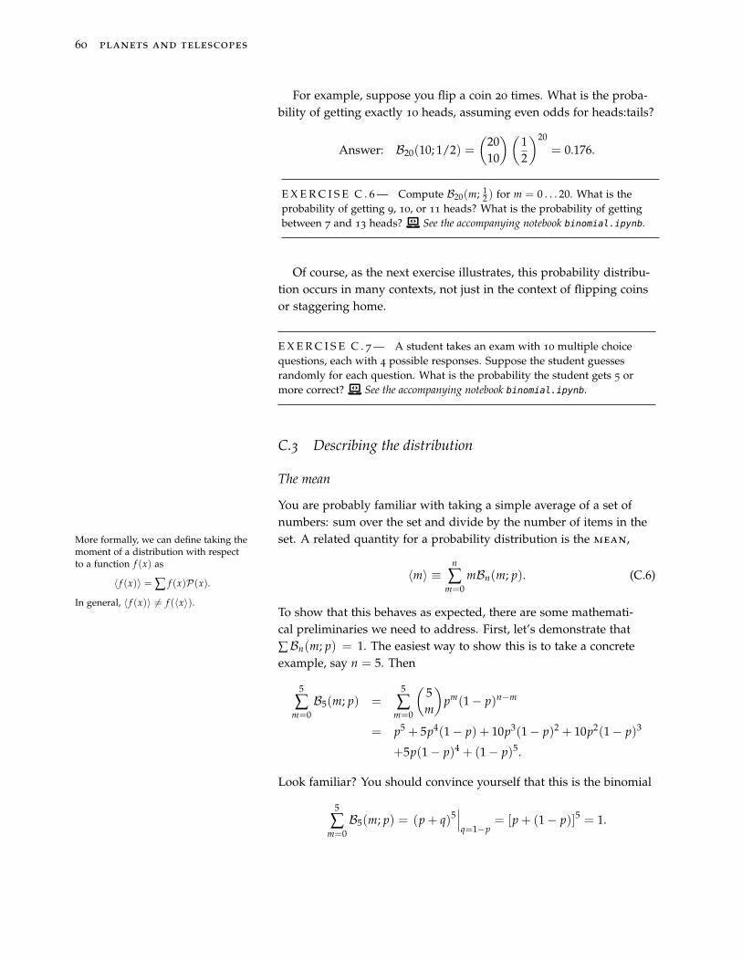
60 planets and telescopes
For example, suppose you flip a coin 20 times. What is the proba-bility of getting exactly 10 heads, assuming even odds for heads:tails?
Answer: B20(10; 1/2) =(
2010
)(12
)20= 0.176.
E X E R C I S E C . 6 — Compute B20(m; 12 ) for m = 0 . . . 20. What is the
probability of getting 9, 10, or 11 heads? What is the probability of gettingbetween 7 and 13 heads? ñ See the accompanying notebook binomial.ipynb.
Of course, as the next exercise illustrates, this probability distribu-tion occurs in many contexts, not just in the context of flipping coinsor staggering home.
E X E R C I S E C . 7 — A student takes an exam with 10 multiple choicequestions, each with 4 possible responses. Suppose the student guessesrandomly for each question. What is the probability the student gets 5 ormore correct? ñ See the accompanying notebook binomial.ipynb.
C.3 Describing the distribution
The mean
You are probably familiar with taking a simple average of a set ofnumbers: sum over the set and divide by the number of items in theset. A related quantity for a probability distribution is the mean,More formally, we can define taking the
moment of a distribution with respectto a function f (x) as
〈 f (x)〉 = ∑ f (x)P(x).
In general, 〈 f (x)〉 6= f (〈x〉).
〈m〉 ≡n
∑m=0
mBn(m; p). (C.6)
To show that this behaves as expected, there are some mathemati-cal preliminaries we need to address. First, let’s demonstrate that∑Bn(m; p) = 1. The easiest way to show this is to take a concreteexample, say n = 5. Then
5
∑m=0B5(m; p) =
5
∑m=0
(5m
)pm(1− p)n−m
= p5 + 5p4(1− p) + 10p3(1− p)2 + 10p2(1− p)3
+5p(1− p)4 + (1− p)5.
Look familiar? You should convince yourself that this is the binomial
5
∑m=0B5(m; p) = (p + q)5
∣∣∣q=1−p
= [p + (1− p)]5 = 1.
probability and statistics 61
We can use this identity, ∑Bn(m; p) = ∑ (nm)pmqn−m = (p + q)n with
q = 1− p, to help us evaluate various sums over the distribution.To evaluate the mean, we first notice that each term in the sum
of equation (C.6) can be written mBn(m; p) = (nm)mpmqn−m. Now
q = 1− p; but if we temporarily let q and p vary independently, wecan write By ∂ f /∂x, we mean, “the derivative
of f with respect to x, holding othervariables fixed.” For example, if f =f (x, y) = x2yey, then ∂ f /∂x = 2xyey
and ∂ f /∂y = x2(1 + y)ey. Sometimeswe write (∂ f /∂x)y just to make it clearwe are holding y fixed.
mBn(m; p) =(
nm
)p(
∂
∂p
)q
pmqn−m = p(
∂
∂p
)q
[(nm
)pmqn−m
].
Hence, the mean is
〈m〉 =n
∑m=0
mBn(m; p)
=
[p(
∂
∂p
)q
n
∑m=0
(nm
)pmqn−m
]q=1−p
=
[p(
∂
∂p
)q(p + q)n
]q=1−p
=[
pn (p + q)n−1]
q=1−p= np. (C.7)
This makes sense: if we flip a fair coin n times, we expect the averagenumber of heads to be n/2. Notice also that for this distribution themean is the value for which the probability is highest.
The standard deviation
Although the mean 〈m〉 = np gives the most likely value, you knowfrom exercise C.6 that there is a substantial probability of getting val-ues other than 〈m〉. What we want to develop is a measure for howtightly the distribution is clustered about the mean. We might wantsomething like 〈m− 〈m〉〉—that is, what is the average differencefrom the mean—but this won’t do: from the definition of the mean,
〈m− 〈m〉〉 = 〈m〉 − 〈m〉 = 0.
We could choose something like 〈|m− 〈m〉|〉, which gives a positive- From the definition of the mean,
〈a + bx〉 = ∑ [(a + bx)P(x)]
= a ∑P(x) + b ∑ xP(x)
= a + b 〈x〉 ,
since ∑P(x) = 1.
definite measure of the width; a more convenient measurement,however, is the root-mean-square (rms) width
√〈(m− 〈m〉)2〉. To
calculate this, let’s first expand the square:⟨(m− 〈m〉)2
⟩=⟨
m2 − 2m 〈m〉+ 〈m〉2⟩=⟨
m2⟩− 〈m〉2 .
To calculate⟨m2⟩ for the binomial distribution, we use a similar trick
from the calculation of 〈m〉:
m2Bn(m; p) = p(
∂
∂p
)q
p(
∂
∂p
)q
[(nm
)pmqn−m
].
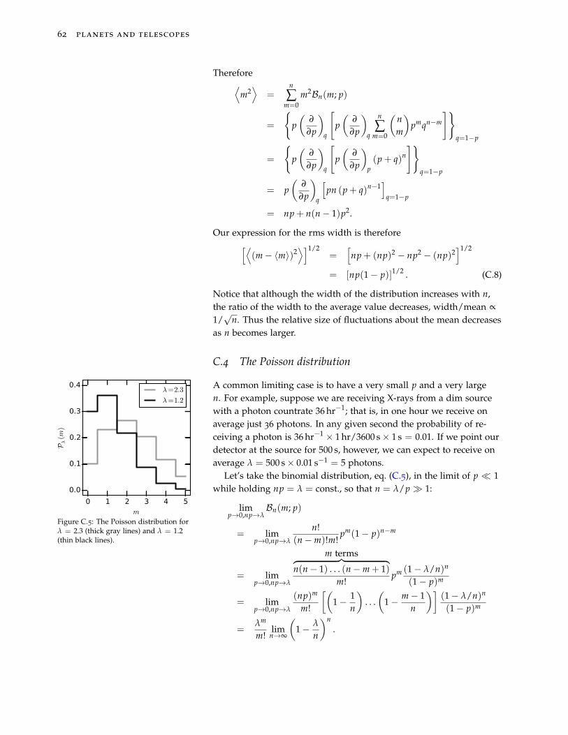
62 planets and telescopes
Therefore⟨m2⟩
=n
∑m=0
m2Bn(m; p)
=
p(
∂
∂p
)q
[p(
∂
∂p
)q
n
∑m=0
(nm
)pmqn−m
]q=1−p
=
p(
∂
∂p
)q
[p(
∂
∂p
)p(p + q)n
]q=1−p
= p(
∂
∂p
)q
[pn (p + q)n−1
]q=1−p
= np + n(n− 1)p2.
Our expression for the rms width is therefore[⟨(m− 〈m〉)2
⟩]1/2=
[np + (np)2 − np2 − (np)2
]1/2
= [np(1− p)]1/2 . (C.8)
Notice that although the width of the distribution increases with n,the ratio of the width to the average value decreases, width/mean ∝1/√
n. Thus the relative size of fluctuations about the mean decreasesas n becomes larger.
C.4 The Poisson distribution
A common limiting case is to have a very small p and a very largen. For example, suppose we are receiving X-rays from a dim sourcewith a photon countrate 36 hr−1; that is, in one hour we receive onaverage just 36 photons. In any given second the probability of re-ceiving a photon is 36 hr−1 × 1 hr/3600 s× 1 s = 0.01. If we point ourdetector at the source for 500 s, however, we can expect to receive onaverage λ = 500 s× 0.01 s−1 = 5 photons.
0 1 2 3 4 5m
0.0
0.1
0.2
0.3
0.4
P λ(m
)
λ=2.3
λ=1.2
Figure C.5: The Poisson distribution forλ = 2.3 (thick gray lines) and λ = 1.2(thin black lines).
Let’s take the binomial distribution, eq. (C.5), in the limit of p 1while holding np = λ = const., so that n = λ/p 1:
limp→0,np→λ
Bn(m; p)
= limp→0,np→λ
n!(n−m)!m!
pm(1− p)n−m
= limp→0,np→λ
m terms︷ ︸︸ ︷n(n− 1) . . . (n−m + 1)
m!pm (1− λ/n)n
(1− p)m
= limp→0,np→λ
(np)m
m!
[(1− 1
n
). . .(
1− m− 1n
)](1− λ/n)n
(1− p)m
=λm
m!lim
n→∞
(1− λ
n
)n.
probability and statistics 63
Recognizing that the last term is just e−λ, we obtain the Poisson
distribution:
P(m, λ) =λm
m!e−λ. (C.9)
Thus in our example, if we have an average photon countrate of36 hr−1 = 0.01 s−1 and we stare at our source for 500 s, then λ = 5 isour expected number of photons, and P(3, λ) would be the probabil-ity of receiving 3 photons in that time.
Not surprisingly, the mean number of events 〈m〉 is
〈m〉 =∞
∑m=0
mλm
m!e−λ
= e−λλd
dλ
∞
∑m=0
λm
m!
= λ.
The standard deviation is
Recall the expansion
eλ =∞
∑m=0
λm
m!.
σ =
√⟨(m− 〈m〉)2
⟩=
√〈m2〉 − 〈m〉2 =
[e−λ
(λ
ddλ
)2 ∞
∑m=0
λm
m!− λ2
]1/2
=
[e−λλ
ddλ
(λeλ)− λ2
]1/2
=√
λ
As with the normal distribution, the ratio of width to mean, σ/ 〈m〉 =1/√
λ, decreases as the mean number of events increases.
E X E R C I S E C . 8 — A high school graduating class has 400 students.What is the probability that 2 people in that class have a birthday on January1? What about 3 students?
E X E R C I S E C . 9 — ñ For a photon countrate of 0.01 s−1, how manyseconds of observation are required so that the mean number of photonsreceived is more than 3σ greater than 0? The notebooksignal-to-noise.ipynb explores the extraction of a weak signal from a noisybackground in more detail.
A historical example of a Poisson distribution is from WWII, whenLondon was targeted by V-1 flying bombs. A total of 537 V-1 bombshit London. To look at where the bombs hit, Clarke7 divided London 7 R. D. Clarke. An application of the
poisson distribution. Journal of theInstitute of Actuaries, 72(3):481, 001 1946.doi: 10.1017/S0020268100035435
into 576 districts, each of 0.25 km2 area. The distribution of bombstrikes went as follows.
no. bombs 0 1 2 3 4 > 5no. districts 229 211 93 35 7 1
64 planets and telescopes
That is, 229 districts were unscathed, 211 districts were hit once, andso on, with one unfortunate district being hit by 7 bombs. Question:were certain districts of London deliberately targeted? Suppose in-stead that the bombs were just launched in the general direction ofLondon and fell randomly over the area. In that case, the probabilityof a district being hit by any one bomb is small—1/576 to be exact.The average number of bombs per district is λ = 537/576 = 0.9323,so we would expect a Poisson distribution if the bombs were dis-tributed randomly, with the expected number of districts hit by mbombs as follows.
N (m) = 576×Pλ(m) = 576× λm
m!e−λ,
m 0 1 2 3 4 5
Pλ(m) 0.3937 0.3670 0.1711 0.0532 0.0124 0.0023
N (m) 227 211 99 31 7 1
This matches the observed distribution well, and the pattern of hitsis therefore consistent with the bombs being scattered randomly overthe London area.88 This was probably small consolation to
the residents of the districts hit multipletimes.
Box C.1 An alternate derivation of the Poisson distribution
The Poisson distribution is frequently encountered whenobserving in X- or γ-rays: the probability of receiving a singlephoton in any given second is small, but over a long periodof time (several thousands of seconds, e.g.) there will be asizable number of photons collected. What is the probabilityof receiving N photons in a given time interval? In this case,we can derive the Poisson distribution independently from thebinomial distribution.
To do so, assume that our time intervals dt are sufficientlyshort that the chance of receiving more than one photon indt is negligible. Then in dt we either receive one photon withprobability µdt 1 or we receive no photons with probability(1− µ)dt. Let us take µ to be a constant, and assume that non-overlapping intervals of time are statistically independent—that is, the chance of receiving a photon in a given intervaldoesn’t depend on what happened in the previous interval.Then there are two ways to receive m photons in a time t + dt:we can receive m photons in a time t and no photons in theinterval (t, t + dt); or we can receive m − 1 photons in a timet and one photon in the interval (t, t + dt). The probability ofreceiving m photons in a time t + dt is the sum of the proba-
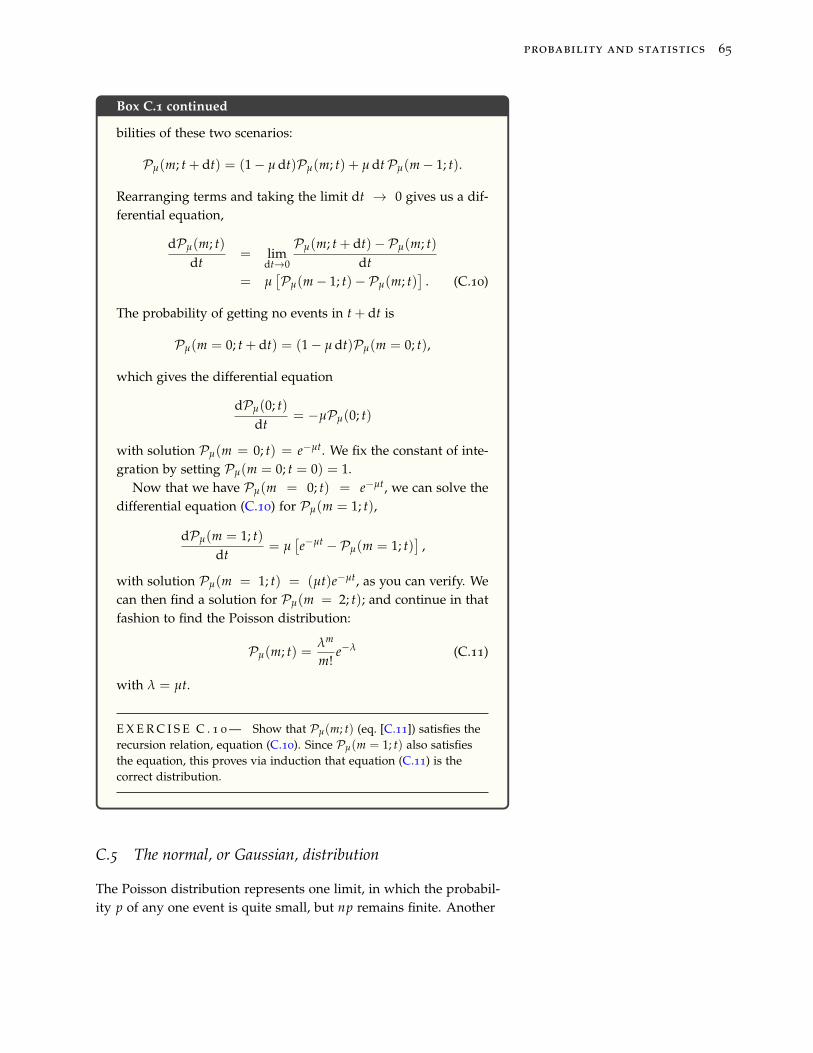
probability and statistics 65
Box C.1 continued
bilities of these two scenarios:
Pµ(m; t + dt) = (1− µ dt)Pµ(m; t) + µ dtPµ(m− 1; t).
Rearranging terms and taking the limit dt → 0 gives us a dif-ferential equation,
dPµ(m; t)dt
= limdt→0
Pµ(m; t + dt)−Pµ(m; t)dt
= µ[Pµ(m− 1; t)−Pµ(m; t)
]. (C.10)
The probability of getting no events in t + dt is
Pµ(m = 0; t + dt) = (1− µ dt)Pµ(m = 0; t),
which gives the differential equation
dPµ(0; t)dt
= −µPµ(0; t)
with solution Pµ(m = 0; t) = e−µt. We fix the constant of inte-gration by setting Pµ(m = 0; t = 0) = 1.
Now that we have Pµ(m = 0; t) = e−µt, we can solve thedifferential equation (C.10) for Pµ(m = 1; t),
dPµ(m = 1; t)dt
= µ[e−µt −Pµ(m = 1; t)
],
with solution Pµ(m = 1; t) = (µt)e−µt, as you can verify. Wecan then find a solution for Pµ(m = 2; t); and continue in thatfashion to find the Poisson distribution:
Pµ(m; t) =λm
m!e−λ (C.11)
with λ = µt.
E X E R C I S E C . 1 0 — Show that Pµ(m; t) (eq. [C.11]) satisfies therecursion relation, equation (C.10). Since Pµ(m = 1; t) also satisfiesthe equation, this proves via induction that equation (C.11) is thecorrect distribution.
C.5 The normal, or Gaussian, distribution
The Poisson distribution represents one limit, in which the probabil-ity p of any one event is quite small, but np remains finite. Another
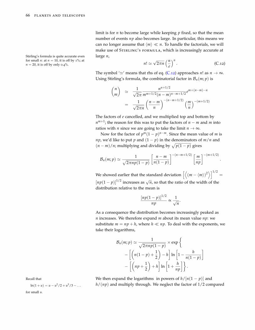
66 planets and telescopes
limit is for n to become large while keeping p fixed, so that the meannumber of events np also becomes large. In particular, this means wecan no longer assume that 〈m〉 n. To handle the factorials, we willmake use of Stirling’s formula, which is increasingly accurate atlarge n,Stirling’s formula is quite accurate even
for small n: at n = 10, it is off by 1%; atn = 20, it is off by only 0.4%. n! '
√2πn
(ne
)n. (C.12)
The symbol ‘'‘ means that rhs of eq. (C.12) approaches n! as n → ∞.Using Stirling’s formula, the combinatorial factor in Bn(m; p) is(
nm
)' 1√
2π
nn+1/2
mm+1/2(n−m)n−m+1/2 em+(n−m)−n
=1√2πn
(n−m
n
)−(n−m+1/2) (mn
)−(m+1/2)
The factors of e cancelled, and we multiplied top and bottom bynm+1; the reason for this was to put the factors of n− m and m intoratios with n since we are going to take the limit n→ ∞.
Now for the factor of pm(1− p)n−m. Since the mean value of m isnp, we’d like to put p and (1− p) in the denominators of m/n and(n−m)/n; multiplying and dividing by
√p(1− p) gives
Bn(m; p) ' 1√2πnp(1− p)
[n−m
n(1− p)
]−(n−m+1/2) [ mnp
]−(m+1/2).
We showed earlier that the standard deviation[⟨
(m− 〈m〉)2⟩]1/2
=
[np(1− p)]1/2 increases as√
n, so that the ratio of the width of thedistribution relative to the mean is
[np(1− p)]1/2
np∝
1√n
.
As a consequence the distribution becomes increasingly peaked asn increases. We therefore expand m about its mean value np: wesubstitute m = np + h, where h np. To deal with the exponents, wetake their logarithms,
Bn(m; p) ' 1√2πnp(1− p)
× exp
−[(
n(1− p) +12
)− h]
ln[
1− hn(1− p)
]−[(
np +12
)+ h]
ln[
1 +h
np
].
We then expand the logarithms in powers of h/[n(1 − p)] andRecall that
ln(1 + u) = u− u2/2 + u3/3− . . .
for small u.
h/(np) and multiply through. We neglect the factor of 1/2 compared
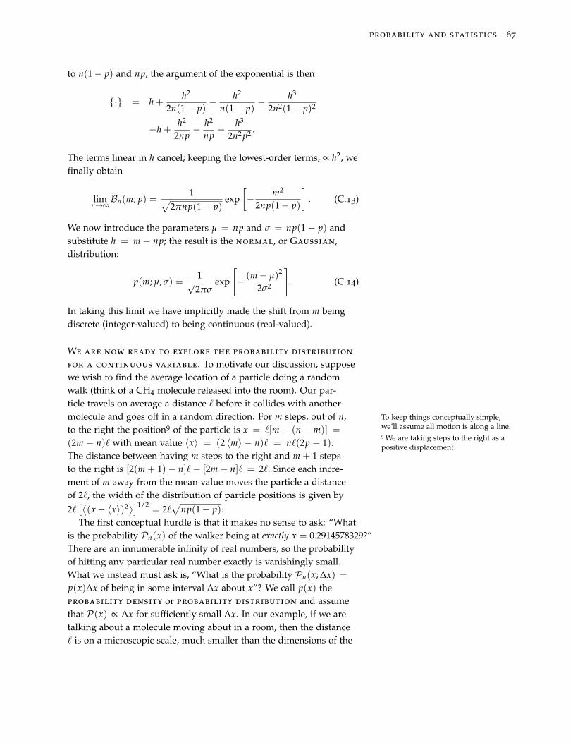
probability and statistics 67
to n(1− p) and np; the argument of the exponential is then
· = h +h2
2n(1− p)− h2
n(1− p)− h3
2n2(1− p)2
−h +h2
2np− h2
np+
h3
2n2 p2 .
The terms linear in h cancel; keeping the lowest-order terms, ∝ h2, wefinally obtain
limn→∞
Bn(m; p) =1√
2πnp(1− p)exp
[− m2
2np(1− p)
]. (C.13)
We now introduce the parameters µ = np and σ = np(1− p) andsubstitute h = m − np; the result is the normal, or Gaussian,distribution:
p(m; µ, σ) =1√2πσ
exp
[− (m− µ)2
2σ2
]. (C.14)
In taking this limit we have implicitly made the shift from m beingdiscrete (integer-valued) to being continuous (real-valued).
We are now ready to explore the probability distribution
for a continuous variable. To motivate our discussion, supposewe wish to find the average location of a particle doing a randomwalk (think of a CH4 molecule released into the room). Our par-ticle travels on average a distance ` before it collides with anothermolecule and goes off in a random direction. For m steps, out of n, To keep things conceptually simple,
we’ll assume all motion is along a line.to the right the position9 of the particle is x = `[m − (n − m)] =9 We are taking steps to the right as apositive displacement.(2m − n)` with mean value 〈x〉 = (2 〈m〉 − n)` = n`(2p − 1).
The distance between having m steps to the right and m + 1 stepsto the right is [2(m + 1) − n]` − [2m − n]` = 2`. Since each incre-ment of m away from the mean value moves the particle a distanceof 2`, the width of the distribution of particle positions is given by2`[⟨(x− 〈x〉)2⟩]1/2
= 2`√
np(1− p).The first conceptual hurdle is that it makes no sense to ask: “What
is the probability Pn(x) of the walker being at exactly x = 0.2914578329?”There are an innumerable infinity of real numbers, so the probabilityof hitting any particular real number exactly is vanishingly small.What we instead must ask is, “What is the probability Pn(x; ∆x) =
p(x)∆x of being in some interval ∆x about x”? We call p(x) theprobability density or probability distribution and assumethat P(x) ∝ ∆x for sufficiently small ∆x. In our example, if we aretalking about a molecule moving about in a room, then the distance` is on a microscopic scale, much smaller than the dimensions of the
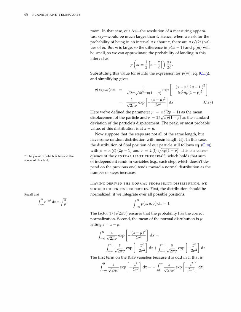
68 planets and telescopes
room. In that case, our ∆x—the resolution of a measuring appara-tus, say—would be much larger than `. Hence, when we ask for theprobability of being in an interval ∆x about x, there are ∆x/(2`) val-ues of m. But m is large, so the difference in p(m + 1) and p(m) willbe small, so we can approximate the probability of landing in thisinterval as
p(
m =12
[n +
x`
]) ∆x2`
.
Substituting this value for m into the expression for p(m), eq. (C.13),and simplifying gives
p(x; µ, σ)dx =1√
2π√
4`2np(1− p)exp
[− (x− n`[2p− 1])2
8`2np(1− p)2
]
=1√2πσ
exp[− (x− µ)2
2σ2
]dx. (C.15)
Here we’ve defined the parameter µ = n`(2p − 1) as the meandisplacement of the particle and σ = 2`
√np(1− p) as the standard
deviation of the particle’s displacement. The peak, or most probablevalue, of this distribution is at x = µ.
Now suppose that the steps are not all of the same length, buthave some random distribution with mean length 〈`〉. In this case,the distribution of final position of our particle still follows eq. (C.15)with µ = n 〈`〉 (2p − 1) and σ = 2 〈l〉
√np(1− p). This is a conse-
quence of the central limit theorem10, which holds that sum10 The proof of which is beyond the
scope of this text, of independent random variables (e.g., each step, which doesn’t de-pend on the previous one) tends toward a normal distribution as thenumber of steps increases.
Having derived the normal probability distribution, we
should check its properties. First, the distribution should benormalized: if we integrate over all possible positions,Recall that∫ ∞
−∞e−βx2
dx =
√π
β.
∫ ∞
−∞p(x; µ, σ)dx = 1.
The factor 1/(√
2πσ) ensures that the probability has the correctnormalization. Second, the mean of the normal distribution is µ:letting z = x− µ,∫ ∞
−∞
x√2πσ
exp
[− (x− µ)2
2σ2
]dx =
∫ ∞
−∞
z√2πσ
exp[− z2
2σ2
]dz +
∫ ∞
−∞
µ√2πσ
exp[− z2
2σ2
]dz
The first term on the RHS vanishes because it is odd in z; that is,∫ 0
−∞
z√2πσ
exp[− z2
2σ2
]dz = −
∫ ∞
0
z√2πσ
exp[− z2
2σ2
]dz.
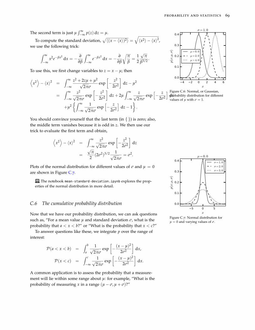
probability and statistics 69
The second term is just µ∫ ∞−∞ p(z)dz = µ.
4 2 0 2 4 6
x
0.0
0.1
0.2
0.3
0.4
p(x
;µ,σ
)
σ= 1. 0
µ= 0. 0
µ= 2. 0
µ= 4. 0
Figure C.6: Normal, or Gaussian,probability distribution for differentvalues of µ with σ = 1.
To compute the standard deviation,√〈(x− 〈x〉)2〉 =
√〈x2〉 − 〈x〉2,
we use the following trick:
∫ ∞
−∞x2e−βx2
dx = − ∂
∂β
∫ ∞
−∞e−βx2
dx = − ∂
∂β
√π
β=
12
√π
β3/2 .
To use this, we first change variables to z = x− µ; then
⟨x2⟩− 〈x〉2 =
∫ ∞
−∞
z2 + 2zµ + µ2√
2πσexp
[− z2
2σ2
]dz− µ2
=∫ ∞
−∞
z2√
2πσexp
[− z2
2σ2
]dz + 2µ
∫ ∞
−∞
z√2πσ
exp[− z
2σ2
]dz
+µ2∫ ∞
−∞
1√2πσ
exp[− z
2σ2
]dz− 1
.
You should convince yourself that the last term (in ) is zero; also,the middle term vanishes because it is odd in z. We then use ourtrick to evaluate the first term and obtain,⟨
x2⟩− 〈x〉2 =
∫ ∞
−∞
z2√
2πσexp
[− z2
2σ2
]dz
=
√π
2(2σ2)3/2 1√
2πσ= σ2.
Plots of the normal distribution for different values of σ and µ = 0are shown in Figure C.7.
ñ The notebook mean-standard-deviation.ipynb explores the prop-erties of the normal distribution in more detail.
5 0 5
x
0.0
0.1
0.2
0.3
0.4
p(x
;µ,σ
)
µ= 0. 0
σ= 1. 0
σ= 2. 0
σ= 3. 0
Figure C.7: Normal distribution forµ = 0 and varying values of σ.
C.6 The cumulative probability distribution
Now that we have our probability distribution, we can ask questionssuch as, “For a mean value µ and standard deviation σ, what is theprobability that a < x < b?” or “What is the probability that x < c?”
To answer questions like these, we integrate p over the range ofinterest:
P(a < x < b) =∫ b
a
1√2πσ
exp[− (x− µ)2
2σ2
]dx,
P(x < c) =∫ c
−∞
1√2πσ
exp[− (x− µ)2
2σ2
]dx.
A common application is to assess the probability that a measure-ment will lie within some range about µ: for example, “What is theprobability of measuring x in a range (µ− σ, µ + σ)?”
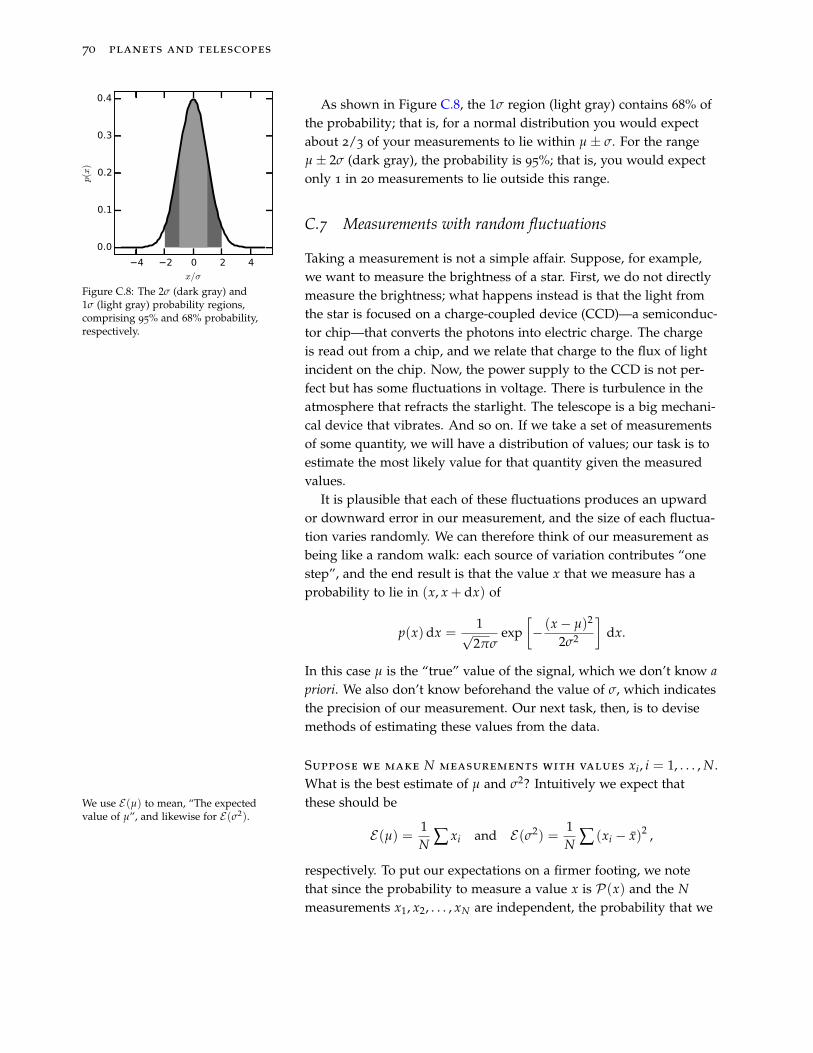
70 planets and telescopes
As shown in Figure C.8, the 1σ region (light gray) contains 68% ofthe probability; that is, for a normal distribution you would expectabout 2/3 of your measurements to lie within µ ± σ. For the rangeµ± 2σ (dark gray), the probability is 95%; that is, you would expectonly 1 in 20 measurements to lie outside this range.
4 2 0 2 4
x/σ
0.0
0.1
0.2
0.3
0.4p(x
)
Figure C.8: The 2σ (dark gray) and1σ (light gray) probability regions,comprising 95% and 68% probability,respectively.
C.7 Measurements with random fluctuations
Taking a measurement is not a simple affair. Suppose, for example,we want to measure the brightness of a star. First, we do not directlymeasure the brightness; what happens instead is that the light fromthe star is focused on a charge-coupled device (CCD)—a semiconduc-tor chip—that converts the photons into electric charge. The chargeis read out from a chip, and we relate that charge to the flux of lightincident on the chip. Now, the power supply to the CCD is not per-fect but has some fluctuations in voltage. There is turbulence in theatmosphere that refracts the starlight. The telescope is a big mechani-cal device that vibrates. And so on. If we take a set of measurementsof some quantity, we will have a distribution of values; our task is toestimate the most likely value for that quantity given the measuredvalues.
It is plausible that each of these fluctuations produces an upwardor downward error in our measurement, and the size of each fluctua-tion varies randomly. We can therefore think of our measurement asbeing like a random walk: each source of variation contributes “onestep”, and the end result is that the value x that we measure has aprobability to lie in (x, x + dx) of
p(x)dx =1√2πσ
exp[− (x− µ)2
2σ2
]dx.
In this case µ is the “true” value of the signal, which we don’t know apriori. We also don’t know beforehand the value of σ, which indicatesthe precision of our measurement. Our next task, then, is to devisemethods of estimating these values from the data.
Suppose we make N measurements with values xi, i = 1, . . . , N.What is the best estimate of µ and σ2? Intuitively we expect thatthese should beWe use E(µ) to mean, “The expected
value of µ”, and likewise for E(σ2).
E(µ) = 1N ∑ xi and E(σ2) =
1N ∑ (xi − x)2 ,
respectively. To put our expectations on a firmer footing, we notethat since the probability to measure a value x is P(x) and the Nmeasurements x1, x2, . . . , xN are independent, the probability that we
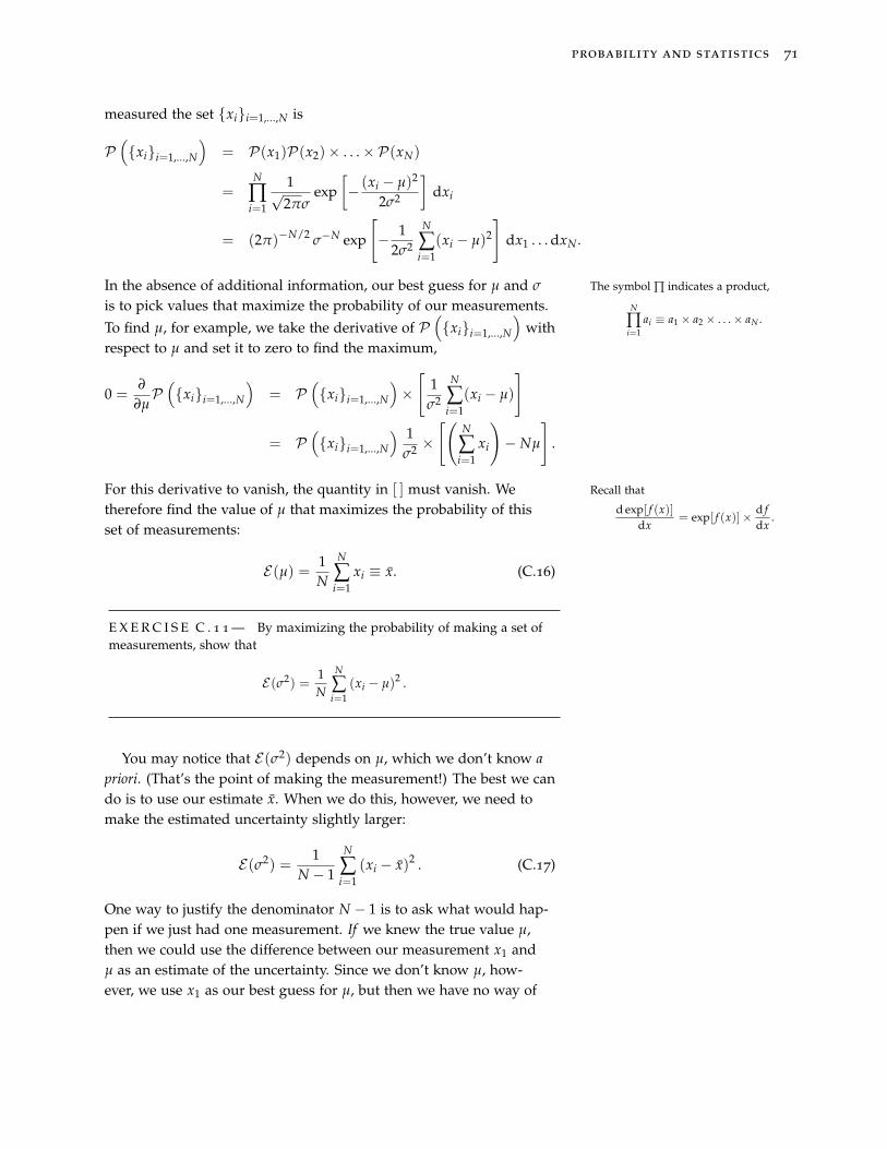
probability and statistics 71
measured the set xii=1,...,N is
P(xii=1,...,N
)= P(x1)P(x2)× . . .×P(xN)
=N
∏i=1
1√2πσ
exp[− (xi − µ)2
2σ2
]dxi
= (2π)−N/2 σ−N exp
[− 1
2σ2
N
∑i=1
(xi − µ)2
]dx1 . . . dxN .
In the absence of additional information, our best guess for µ and σ The symbol ∏ indicates a product,
N
∏i=1
ai ≡ a1 × a2 × . . .× aN .is to pick values that maximize the probability of our measurements.
To find µ, for example, we take the derivative of P(xii=1,...,N
)with
respect to µ and set it to zero to find the maximum,
0 =∂
∂µP(xii=1,...,N
)= P
(xii=1,...,N
)×[
1σ2
N
∑i=1
(xi − µ)
]
= P(xii=1,...,N
) 1σ2 ×
[(N
∑i=1
xi
)− Nµ
].
For this derivative to vanish, the quantity in [ ] must vanish. We Recall that
d exp[ f (x)]dx
= exp[ f (x)]× d fdx
.therefore find the value of µ that maximizes the probability of thisset of measurements:
E(µ) = 1N
N
∑i=1
xi ≡ x. (C.16)
E X E R C I S E C . 1 1 — By maximizing the probability of making a set ofmeasurements, show that
E(σ2) =1N
N
∑i=1
(xi − µ)2 .
You may notice that E(σ2) depends on µ, which we don’t know apriori. (That’s the point of making the measurement!) The best we cando is to use our estimate x. When we do this, however, we need tomake the estimated uncertainty slightly larger:
E(σ2) =1
N − 1
N
∑i=1
(xi − x)2 . (C.17)
One way to justify the denominator N − 1 is to ask what would hap-pen if we just had one measurement. If we knew the true value µ,then we could use the difference between our measurement x1 andµ as an estimate of the uncertainty. Since we don’t know µ, how-ever, we use x1 as our best guess for µ, but then we have no way of
72 planets and telescopes
independently assessing the uncertainty. The fact that eq. (C.17) re-quires N ≥ 2 reflects this constraint. See Box C.2 for a derivation ofeq. (C.17).
In practice, the difference in the denominator between N andN − 1 is not usually important11.11 To quote Press et al. [2007], “if the
difference between N and N − 1 [in theformula for E(σ2)] ever matters to you,then you are probably up to no good.”
ñ The notebook distribution.ipynb explores further how one as-sesses the quality of these estimates of the mean and standard deviationfrom a set of measurements. This is followed by fitting-data.ipynb,which looks at how one tests how well a set of measurements conformsto a hypothesis.
Box C.2 A derivation of E(σ2)
To understand why the denominator of eq. (C.17) is N − 1instead of N, let’s imagine that there is an infinitude of copiesof our universe, and in each copy, our set of measurementsis performed. The mean (averaged over all universes) of x isthen
〈x〉 =⟨
1N
N
∑i=1
xi
⟩=
1N
N
∑i=1〈xi〉 = 〈x〉 = µ.
(Since each variable is drawn from the same distribution,∑N
i=1 〈xi〉 = N 〈x〉.) This is what we expect, and further justi-fies our using x as an estimate for µ. It doesn’t mean, however,that x = µ for our universe.
Now, let’s do the same thought experiment for ∑Ni=1(xi −
x)2. Expanding the square,⟨N
∑i=1
(xi − x)2
⟩=
⟨N
∑i=1
(x2
i − 2xi x + x2)⟩
=
⟨N
∑i=1
x2i − Nx2
⟩.
(C.18)Here
N
∑i=1
2xi x = 2xN
∑i=1
xi = 2Nx2
andN
∑i=1
x2 = Nx2.
Next, we expand x2. There are N2 terms:
x2 =1N(x1 + x2 + . . . + xN)×
1N(x1 + x2 + . . . + xN)
=1
N2
N terms︷ ︸︸ ︷(
x21 + x2
2 + . . . + x2N
)
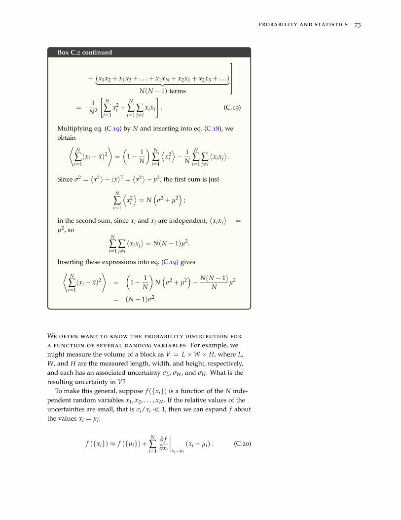
probability and statistics 73
Box C.2 continued
+ (x1x2 + x1x3 + . . . + x1xN + x2x1 + x2x3 + . . .)︸ ︷︷ ︸N(N − 1) terms
=
1N2
[N
∑i=1
x2i +
N
∑i=1
∑j 6=i
xixj
]. (C.19)
Multiplying eq. (C.19) by N and inserting into eq. (C.18), weobtain⟨
N
∑i=1
(xi − x)2
⟩=
(1− 1
N
) N
∑i=1
⟨x2
i
⟩− 1
N
N
∑i=1
∑j 6=i
⟨xixj
⟩.
Since σ2 =⟨
x2⟩− 〈x〉2 =⟨
x2⟩− µ2, the first sum is just
N
∑i=1
⟨x2
i
⟩= N
(σ2 + µ2
);
in the second sum, since xi and xj are independent,⟨
xixj⟩
=
µ2, soN
∑i=1
∑j 6=i
⟨xixj
⟩= N(N − 1)µ2.
Inserting these expressions into eq. (C.19) gives⟨N
∑i=1
(xi − x)2
⟩=
(1− 1
N
)N(
σ2 + µ2)− N(N − 1)
Nµ2
= (N − 1)σ2.
We often want to know the probability distribution for
a function of several random variables. For example, wemight measure the volume of a block as V = L ×W × H, where L,W, and H are the measured length, width, and height, respectively,and each has an associated uncertainty σL, σW , and σH . What is theresulting uncertainty in V?
To make this general, suppose f (xi) is a function of the N inde-pendent random variables x1, x2, . . . , xN . If the relative values of theuncertainties are small, that is σi/xi 1, then we can expand f aboutthe values xi = µi:
f (xi) ≈ f (µi) +N
∑i=1
∂ f∂xi
∣∣∣∣xi=µi
(xi − µi) . (C.20)
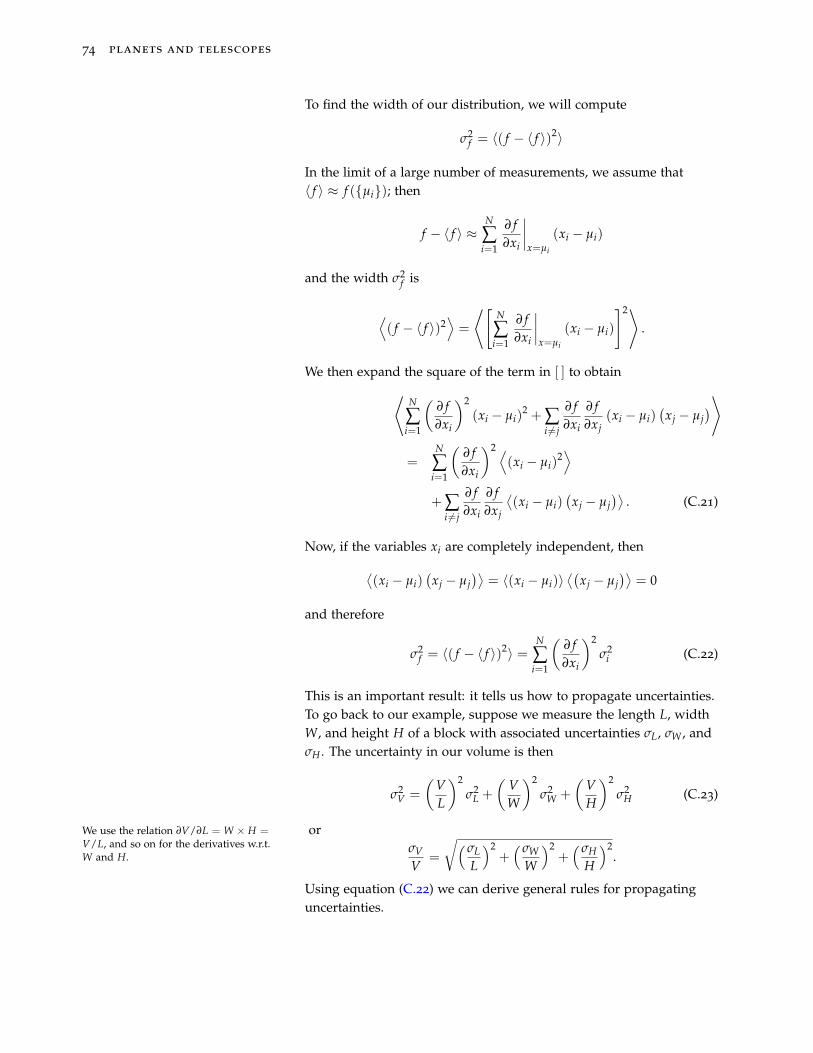
74 planets and telescopes
To find the width of our distribution, we will compute
σ2f = 〈( f − 〈 f 〉)2〉
In the limit of a large number of measurements, we assume that〈 f 〉 ≈ f (µi); then
f − 〈 f 〉 ≈N
∑i=1
∂ f∂xi
∣∣∣∣x=µi
(xi − µi)
and the width σ2f is
⟨( f − 〈 f 〉)2
⟩=
⟨[N
∑i=1
∂ f∂xi
∣∣∣∣x=µi
(xi − µi)
]2⟩.
We then expand the square of the term in [ ] to obtain⟨N
∑i=1
(∂ f∂xi
)2
(xi − µi)2 + ∑
i 6=j
∂ f∂xi
∂ f∂xj
(xi − µi)(xj − µj
)⟩
=N
∑i=1
(∂ f∂xi
)2 ⟨(xi − µi)
2⟩
+∑i 6=j
∂ f∂xi
∂ f∂xj
⟨(xi − µi)
(xj − µj
)⟩. (C.21)
Now, if the variables xi are completely independent, then⟨(xi − µi)
(xj − µj
)⟩= 〈(xi − µi)〉
⟨(xj − µj
)⟩= 0
and therefore
σ2f = 〈( f − 〈 f 〉)2〉 =
N
∑i=1
(∂ f∂xi
)2σ2
i (C.22)
This is an important result: it tells us how to propagate uncertainties.To go back to our example, suppose we measure the length L, widthW, and height H of a block with associated uncertainties σL, σW , andσH . The uncertainty in our volume is then
σ2V =
(VL
)2σ2
L +
(VW
)2σ2
W +
(VH
)2σ2
H (C.23)
orWe use the relation ∂V/∂L = W × H =V/L, and so on for the derivatives w.r.t.W and H.
σVV
=
√(σLL
)2+(σW
W
)2+(σH
H
)2.
Using equation (C.22) we can derive general rules for propagatinguncertainties.
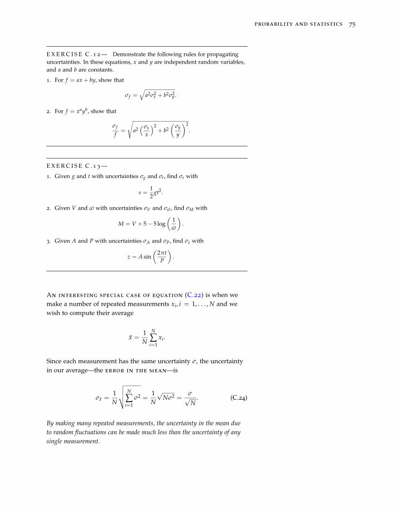
probability and statistics 75
E X E R C I S E C . 1 2 — Demonstrate the following rules for propagatinguncertainties. In these equations, x and y are independent random variables,and a and b are constants.
1. For f = ax + by, show that
σf =√
a2σ2x + b2σ2
y .
2. For f = xayb, show that
σf
f=
√a2(σx
x
)2+ b2
(σy
y
)2.
E X E R C I S E C . 1 3 —
1. Given g and t with uncertainties σg and σt, find σs with
s =12
gt2.
2. Given V and v with uncertainties σV and σv , find σM with
M = V + 5− 5 log(
1v
).
3. Given A and P with uncertainties σA and σP, find σz with
z = A sin(
2πtP
).
An interesting special case of equation (C.22) is when wemake a number of repeated measurements xi, i = 1, . . . , N and wewish to compute their average
x =1N
N
∑i=1
xi.
Since each measurement has the same uncertainty σ, the uncertaintyin our average—the error in the mean—is
σx =1N
√√√√ N
∑i=1
σ2 =1N
√Nσ2 =
σ√N
. (C.24)
By making many repeated measurements, the uncertainty in the mean dueto random fluctuations can be made much less than the uncertainty of anysingle measurement.
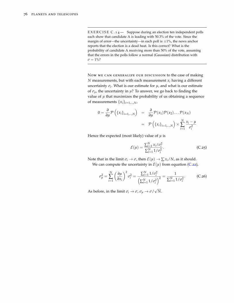
76 planets and telescopes
E X E R C I S E C . 1 4 — Suppose during an election ten independent pollseach show that candidate A is leading with 50.3% of the vote. Since themargin of error—the uncertainty—in each poll is ±1%, the news anchorreports that the election is a dead heat. Is this correct? What is theprobability of candidate A receiving more than 50% of the vote, assumingthat the errors in the polls follow a normal (Gaussian) distribution withσ = 1%?
Now we can generalize our discussion to the case of makingN measurements, but with each measurement xi having a differentuncertainty σi. What is our estimate for µ, and what is our estimateof σµ, the uncertainty in µ? To answer, we go back to finding thevalue of µ that maximizes the probability of us obtaining a sequenceof measurements xii=1,...,N ,
0 =∂
∂µP(xii=1,...,N
)=
∂
∂µP(x1)P(x2) . . .P(xN)
= P(xii=1,...,N
)×
N
∑i=1
xi − µ
σ2i
Hence the expected (most likely) value of µ is
E(µ) = ∑Ni=1 xi/σ2
i
∑Ni=1 1/σ2
i. (C.25)
Note that in the limit σi → σ, then E(µ)→ ∑ xi/N, as it should.We can compute the uncertainty in E(µ) from equation (C.22),
σ2µ =
N
∑i=1
(∂µ
∂xi
)2σ2
i =∑N
i=1 1/σ2i(
∑Ni=1 1/σ2
i
)2 =1
∑Ni=1 1/σ2
i. (C.26)
As before, in the limit σi → σ, σµ → σ/√
N.
Bibliography
Jeffrey O. Bennett, Megan O. Donahue, Nicholas Schneider, and MarkVoit. The Cosmic Perspective. Addison-Wesley, 7th edition, 2013.
James Binney and Michael Merrifield. Galactic Astronomy. PrincetonUniversity Press, 1998.
Edward F. Brown, Laura Chomiuk, Laura Shishkovsky, and AndrewBundas. Development of a sophomore level astronomy courseon planets and telescopes. White paper detailing revisions toAST 208, MSU, 2015. URL https://www.authorea.com/19544/
7GTRKXg6i69rNPihL7S99g.
R. D. Clarke. An application of the poisson distribution. Jour-nal of the Institute of Actuaries, 72(3):481, 001 1946. doi:10.1017/S0020268100035435.
Richard Courant, Herbert Robbins, and Ian Stewart. What is Mathe-matics? Oxford University Press, 2d edition, 1996.
Richard Durrett. The Essentials of Probability. Duxbury Press, Belmont,CA, 1994.
Enrico Fermi. Thermodynamics. Dover, 1956.
J. Laskar and M. Gastineau. Existence of collisional trajectories ofMercury, Mars and Venus with the Earth. Nature, 459:817–819, June2009. doi: 10.1038/nature08096.
Jack J. Lissauer and Imke de Pater. Fundamental Planetary Science:Physics, Chemistry and Habitability. Cambridge University Press,2013.
William H. Press, Saul E. Teukolsky, William T. Vetterling, andBrian P. Flannery. Numerical Recipes. Cambridge University Press,3d edition, 2007.
Barbara Ryden and Bradley M. Peterson. Foundations of Astrophysics.Addison-Wesley, 2010.
78 planets and telescopes
John R. Taylor. An Introduction to Error Analysis. University ScienceBooks, Sausalito, CA, 2nd edition, 1997.
W. R. Ward and D. P. Hamilton. Tilting Saturn. I. Analytic Model. As-tron. Journ., 128:2501–2509, November 2004. doi: 10.1086/424533.
J. Zachos, M. Pagani, L. Sloan, E. Thomas, and K. Billups. Trends,Rhythms, and Aberrations in Global Climate 65 Ma to Present.Science, 292:686–693, April 2001. doi: 10.1126/science.1059412.