Plasma Physics and Controlled Fusion

PAPER

Interpretation of machine-learning-baseddisruption models for plasma controlTo cite this article: Matthew S Parsons 2017 Plasma Phys. Control. Fusion 59 085001

 

View the article online for updates and enhancements.

Related contentAdaptive high learning rate probabilisticdisruption predictors from scratch for thenext generation of tokamaksJ. Vega, A. Murari, S. Dormido-Canto et al.

-

An advanced disruption predictor for JETtested in a simulated real-timeenvironmentG.A. Rattá, J. Vega, A. Murari et al.

-

Development of an efficient real-timedisruption predictor from scratch on JETand implications for ITERS. Dormido-Canto, J. Vega, J.M. Ramírezet al.

-

This content was downloaded from IP address 128.174.163.157 on 13/06/2018 at 19:47

Interpretation of machine-learning-baseddisruption models for plasma control

Matthew S Parsons

Department of Nuclear, Plasma, and Radiological Engineering, University of Illinois at Urbana-Champaign, Urbana, IL, United States of America

E-mail: parsons6@illinois.edu

Received 2 February 2017, revised 30 March 2017Accepted for publication 11 May 2017Published 5 June 2017

AbstractWhile machine learning techniques have been applied within the context of fusion for predictingplasma disruptions in tokamaks, they are typically interpreted with a simple ‘yes/no’ predictionor perhaps a probability forecast. These techniques take input signals, which could be real-timesignals from machine diagnostics, to make a prediction of whether a transient event will occur. Amajor criticism of these methods is that, due to the nature of machine learning, there is no clearcorrelation between the input signals and the output prediction result. Here is proposed a simplemethod that could be applied to any existing prediction model to determine how sensitive thestate of a plasma is at any given time with respect to the input signals. This is accomplished bycomputing the gradient of the decision function, which effectively identifies the quickest pathaway from a disruption as a function of the input signals and therefore could be used in a plasmacontrol setting to avoid them. A numerical example is provided for illustration based on asupport vector machine model, and the application to real data is left as an open opportunity.

Keywords: plasma disruptions, disruption prediction, disruption avoidance, plasma control,machine learning

(Some figures may appear in colour only in the online journal)

1. Introduction

In a tokamak, it is possible for the plasma to suddenly escapeits confinement in an event known as a disruption [1, 2]. Thissudden loss of confinement results in thermal and magneticloads on the walls, and potentially the formation of electroncurrents with relativistic energies, which can seriouslydamage the machine. In order for the tokamak to be a viabledesign for a fusion power plant, it must be possible to avoid,or at least reliably mitigate, the effects of disruptions. Evenbefore a power plant, the need for minimizing disruptions inITER is severe [3]. Since avoidance and mitigation techniquesare inherently more effective when more warning time isgiven for them to be enacted, a great deal of attention hasbeen given to the prediction of disruptions.

There are a large variety of phenomena which lead up todisruptions, which makes their prediction a significant chal-lenge. However, there is a wealth of experimental data thathas been accumulated on disruptions from experimentsaround the world, and this data provides a place to search for

answers. To help make sense of this wealth of disruption data,one can employ the tools of machine learning to search forpatterns and construct models to predict the occurrence ofdisruptions.

A lot of promising work has been done in applyingmachine learning techniques to the problem of disruptionprediction. This work is based on the idea that disruptivedischarges must exhibit some characteristics, just before thedisruption occurs, which distinguish them from non-dis-ruptive discharges. Using diagnostic measurements takenfrom both disruptive and non-disruptive plasmas, a machinelearning algorithm constructs a model which separates thedisruptive and non-disruptive plasma conditions as clearly aspossible. The model will then give a prediction, either interms of a probability or a simple yes/no response, of whethera disruption will occur for a given set of input variables. Inthis decade, this has been demonstrated using LogisticRegression on AUG [4], Multilayer Perceptron Neural Net-works on AUG [5, 6] and separately on J-TEXT [7], SupportVector Machines on JET [8–11], and Adaptive Venn

Plasma Physics and Controlled Fusion

Plasma Phys. Control. Fusion 59 (2017) 085001 (5pp) https://doi.org/10.1088/1361-6587/aa72a3

0741-3335/17/085001+05$33.00 © 2017 IOP Publishing Ltd Printed in the UK1

Predictors on JET [12]. In testing these machine-learning-based disruption models on other archived and even real-timedata, prediction success rates have been demonstrated near90%, with just a few percent of false alarms.

A major criticism of these approaches is that they fail tomake a clear correlation between their inputs and outputs, asis inherently the nature of machine learning models. Thiscriticism has continued to dissuade a more serious pursuit todevelop these techniques, which are often viewed as beingout-of-place in the plasma physics community. While precisescaling-law-type relationships are likely not to be recoverablefrom these models, it still is possible to extract some infor-mation about how the input parameters affect the output. Hereis described a new way to interpret machine-learning-baseddisruption prediction models, and some implications of thisinterpretation for plasma control applications. While the focuswill be on disruptions, it is worth noting that this type ofanalysis could be applied to any situation where differentplasma states are tracked, such as ELM regime classifica-tion [13].

2. Classification model interpretation

To begin, suppose that a disruption prediction model existswhich can identify whether a plasma will disrupt or not basedon the input of n features describing the state of the plasma.These features, which may include quantities like the plasmacurrent and density, combine to form a so-called featurevector Î Ì Rx n. For any feature vector x in the domain, a decision function ( )f x can determine where x is withrespect to the boundary between the two classes.

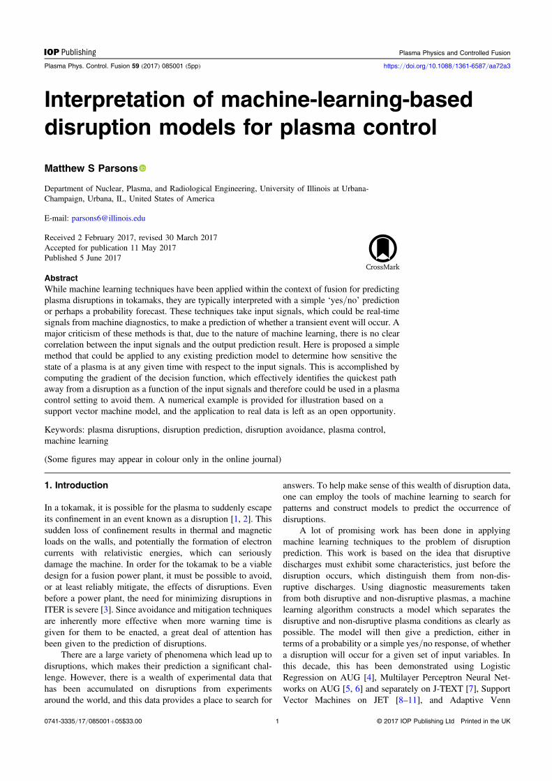
As a simple toy model, consider a system of two classesA and B (or disruptive and non-disruptive) represented bytwo features Î [ ]x 0, 11 and Î [ ]x 0, 12 . The number ofdimensions used in disruption prediction work is typicallysomething like 14, though two will provide a more tangibleillustration. Here, a decision function is produced with asupport vector machine algorithm [14], which takes a set of‘training’ points and pulls out the ones which best separatethe two classes. The set of points forming the boundarybetween the two classes are called support vectors, and theseare used by the decision function to determine the class of anynew point. A set of Support Vectors separating classes A andB can be seen in figure 1.

During a plasma discharge, the state of the plasma willevolve through the feature space. Since the features arealways normalized to represent their individual statisticalranges, the trajectory will be reasonably smooth with respectto the entire domain. To simulate this motion through thefeature space, consider moving in the 2D plane with anattractive x1 2 force at the origin. By ‘launching’ differenttrajectories through the feature space, one can examine dif-ferent scenarios of approaching the boundary. The decisionfunction can then be exploited to better understand what ishappening along the trajectory and how one might use thatinformation to make control decisions.

As a first example, consider Trajectory 1 as depicted infigure 2, which collides with the boundary after triggering twowarning alarms. Alarm 1 is the maximal distance of anysupport vector from the boundary, and Alarm 2 is twice thisvalue. There is a significant uncertainty in the ability of the

Figure 1. A set of 10 000 training points is randomly generated on a2D grid spanning 0 to 1, and the points are assigned to one of twoclasses, A (red) or B (blue), based on their location. An SVM modelwith a gaussian kernel is trained on this data, and the points chosenas support vectors (purple) mark the noisy boundary between the twoclasses. In practice, the noisiness of the boundary depends entirelyon the particular features chosen, and ideally the boundary could bedrawn as a distinct line.

Figure 2. Trajectory 1 through feature space results in a collisionwith the boundary after several warning alarms.

2

Plasma Phys. Control. Fusion 59 (2017) 085001 M S Parsons

decision function to correctly classify points inside the marginof support vectors, so Alarm 1 marks the edge of a greyregion for prediction. If a collision with the boundary is to beavoided, this would be the last opportunity to take an action.

Everywhere along this trajectory, the decision functionoutputs a measurement of how far a given point is from theboundary. Whether this distance is positive or negativeidentifies which side of the boundary it is on, and hencewhich class it belongs to. Disruption prediction researchtypically only utilizes the class information, but there is muchto be gained by considering the distance measurement itself. Itis important to note that this distance is not a distance in thefeature space, but is a measure of how far away the decisionfunction perceives the boundary to be. In practice, the preciselocation of the boundary would not be known or a statisticalmodel would not be needed in the first place, so it is notambiguous to continue to refer to this simply as the distancefrom the boundary.

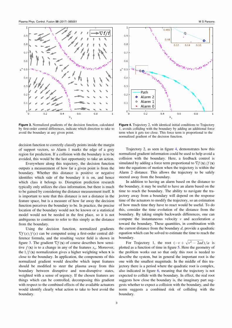
Using the decision function, normalized gradients ( ) ( )f x f x can be computed using a first-order central dif-ference formula, and the resulting vector field is shown infigure 3. The gradient ( )f x of course describes how sensi-tive ( )f x is to a change in any of the features xn. Moreover,the ( )f x1 normalization gives a higher weighting when x isclose to the boundary. In application, the components of thisnormalized gradient would describe which input featuresshould be modified to steer the plasma away from thisboundary between disruptive and non-disruptive states,weighted with a sense of urgency. If the chosen features arethings which can be controlled, decomposing this gradientwith respect to the combined effects of the available actuatorswould identify clearly what action to take to best avoid theboundary.

Trajectory 2, as seen in figure 4, demonstrates how thisnormalized gradient information could be used to help avoid acollision with the boundary. Here, a feedback control issimulated by adding a force term proportional to ( ) ( )f fx xinto the equations of motion when the trajectory is within theAlarm 2 distance. This allows the trajectory to be safelysteered away from the boundary.

In addition to having an alarm based on the distance tothe boundary, it may be useful to have an alarm based on thetime to reach the boundary. The ability to navigate the tra-jectory away from a boundary will depend on the responsetime of the actuators to modify the trajectory, so an estimationof how much time they have to react would be useful. To dothis, consider the time evolution of the distance from theboundary. By taking simple backwards differences, one cancompute the instantaneous velocity v and acceleration atoward the boundary. These quantities, in combination withthe current distance from the boundary d, provide a quadraticequation which can be solved to estimate the time to reach theboundary.

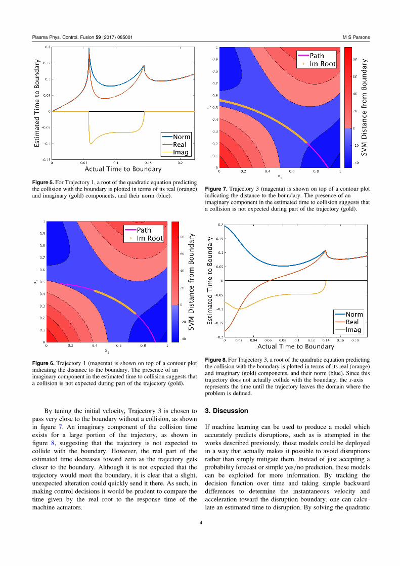
For Trajectory 1, the root - + -( )v v ad a22 isplotted as a function of time in figure 5. Here the geometry ofthe problem works out so that only this root is needed todescribe the system, but in general the important root is theone with the smallest magnitude. In the middle of this tra-jectory there is a period where the quadratic root is complex,also indicated in figure 6, meaning that the trajectory is notexpected to collide with the boundary. In effect, the real rootsuggests how close the boundary is, the imaginary part sug-gests whether to expect a collision with the boundary, and thenorm suggests a combined risk of colliding with theboundary.

Figure 3. Normalized gradients of the decision function, calculatedby first-order central differences, indicate which direction to take toavoid the boundary at any given point.

Figure 4. Trajectory 2, with identical initial conditions to Trajectory1, avoids colliding with the boundary by adding an additional forceterm when it gets too close. This force term is proportional to thenormalized gradient of the decision function.

3

Plasma Phys. Control. Fusion 59 (2017) 085001 M S Parsons

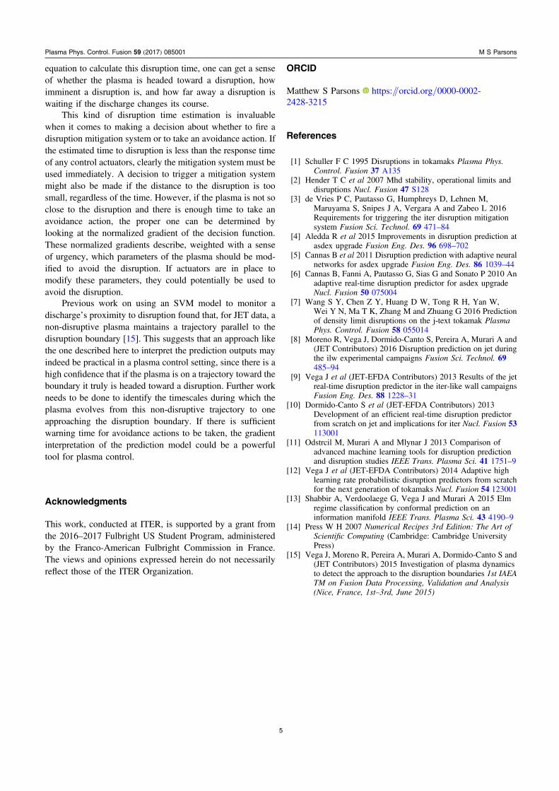
By tuning the initial velocity, Trajectory 3 is chosen topass very close to the boundary without a collision, as shownin figure 7. An imaginary component of the collision timeexists for a large portion of the trajectory, as shown infigure 8, suggesting that the trajectory is not expected tocollide with the boundary. However, the real part of theestimated time decreases toward zero as the trajectory getscloser to the boundary. Although it is not expected that thetrajectory would meet the boundary, it is clear that a slight,unexpected alteration could quickly send it there. As such, inmaking control decisions it would be prudent to compare thetime given by the real root to the response time of themachine actuators.

3. Discussion

If machine learning can be used to produce a model whichaccurately predicts disruptions, such as is attempted in theworks described previously, those models could be deployedin a way that actually makes it possible to avoid disruptionsrather than simply mitigate them. Instead of just accepting aprobability forecast or simple yes/no prediction, these modelscan be exploited for more information. By tracking thedecision function over time and taking simple backwarddifferences to determine the instantaneous velocity andacceleration toward the disruption boundary, one can calcu-late an estimated time to disruption. By solving the quadratic

Figure 5. For Trajectory 1, a root of the quadratic equation predictingthe collision with the boundary is plotted in terms of its real (orange)and imaginary (gold) components, and their norm (blue).

Figure 6. Trajectory 1 (magenta) is shown on top of a contour plotindicating the distance to the boundary. The presence of animaginary component in the estimated time to collision suggests thata collision is not expected during part of the trajectory (gold).

Figure 7. Trajectory 3 (magenta) is shown on top of a contour plotindicating the distance to the boundary. The presence of animaginary component in the estimated time to collision suggests thata collision is not expected during part of the trajectory (gold).

Figure 8. For Trajectory 3, a root of the quadratic equation predictingthe collision with the boundary is plotted in terms of its real (orange)and imaginary (gold) components, and their norm (blue). Since thistrajectory does not actually collide with the boundary, the x-axisrepresents the time until the trajectory leaves the domain where theproblem is defined.

4

Plasma Phys. Control. Fusion 59 (2017) 085001 M S Parsons

equation to calculate this disruption time, one can get a senseof whether the plasma is headed toward a disruption, howimminent a disruption is, and how far away a disruption iswaiting if the discharge changes its course.

This kind of disruption time estimation is invaluablewhen it comes to making a decision about whether to fire adisruption mitigation system or to take an avoidance action. Ifthe estimated time to disruption is less than the response timeof any control actuators, clearly the mitigation system must beused immediately. A decision to trigger a mitigation systemmight also be made if the distance to the disruption is toosmall, regardless of the time. However, if the plasma is not soclose to the disruption and there is enough time to take anavoidance action, the proper one can be determined bylooking at the normalized gradient of the decision function.These normalized gradients describe, weighted with a senseof urgency, which parameters of the plasma should be mod-ified to avoid the disruption. If actuators are in place tomodify these parameters, they could potentially be used toavoid the disruption.

Previous work on using an SVM model to monitor adischarge’s proximity to disruption found that, for JET data, anon-disruptive plasma maintains a trajectory parallel to thedisruption boundary [15]. This suggests that an approach likethe one described here to interpret the prediction outputs mayindeed be practical in a plasma control setting, since there is ahigh confidence that if the plasma is on a trajectory toward theboundary it truly is headed toward a disruption. Further workneeds to be done to identify the timescales during which theplasma evolves from this non-disruptive trajectory to oneapproaching the disruption boundary. If there is sufficientwarning time for avoidance actions to be taken, the gradientinterpretation of the prediction model could be a powerfultool for plasma control.

Acknowledgments

This work, conducted at ITER, is supported by a grant fromthe 2016–2017 Fulbright US Student Program, administeredby the Franco-American Fulbright Commission in France.The views and opinions expressed herein do not necessarilyreflect those of the ITER Organization.

ORCID

Matthew S Parsons https://orcid.org/0000-0002-2428-3215

References

[1] Schuller F C 1995 Disruptions in tokamaks Plasma Phys.Control. Fusion 37 A135

[2] Hender T C et al 2007 Mhd stability, operational limits anddisruptions Nucl. Fusion 47 S128

[3] de Vries P C, Pautasso G, Humphreys D, Lehnen M,Maruyama S, Snipes J A, Vergara A and Zabeo L 2016Requirements for triggering the iter disruption mitigationsystem Fusion Sci. Technol. 69 471–84

[4] Aledda R et al 2015 Improvements in disruption prediction atasdex upgrade Fusion Eng. Des. 96 698–702

[5] Cannas B et al 2011 Disruption prediction with adaptive neuralnetworks for asdex upgrade Fusion Eng. Des. 86 1039–44

[6] Cannas B, Fanni A, Pautasso G, Sias G and Sonato P 2010 Anadaptive real-time disruption predictor for asdex upgradeNucl. Fusion 50 075004

[7] Wang S Y, Chen Z Y, Huang D W, Tong R H, Yan W,Wei Y N, Ma T K, Zhang M and Zhuang G 2016 Predictionof density limit disruptions on the j-text tokamak PlasmaPhys. Control. Fusion 58 055014

[8] Moreno R, Vega J, Dormido-Canto S, Pereira A, Murari A and(JET Contributors) 2016 Disruption prediction on jet duringthe ilw experimental campaigns Fusion Sci. Technol. 69485–94

[9] Vega J et al (JET-EFDA Contributors) 2013 Results of the jetreal-time disruption predictor in the iter-like wall campaignsFusion Eng. Des. 88 1228–31

[10] Dormido-Canto S et al (JET-EFDA Contributors) 2013Development of an efficient real-time disruption predictorfrom scratch on jet and implications for iter Nucl. Fusion 53113001

[11] Odstrcil M, Murari A and Mlynar J 2013 Comparison ofadvanced machine learning tools for disruption predictionand disruption studies IEEE Trans. Plasma Sci. 41 1751–9

[12] Vega J et al (JET-EFDA Contributors) 2014 Adaptive highlearning rate probabilistic disruption predictors from scratchfor the next generation of tokamaks Nucl. Fusion 54 123001

[13] Shabbir A, Verdoolaege G, Vega J and Murari A 2015 Elmregime classification by conformal prediction on aninformation manifold IEEE Trans. Plasma Sci. 43 4190–9

[14] Press W H 2007 Numerical Recipes 3rd Edition: The Art ofScientific Computing (Cambridge: Cambridge UniversityPress)

[15] Vega J, Moreno R, Pereira A, Murari A, Dormido-Canto S and(JET Contributors) 2015 Investigation of plasma dynamicsto detect the approach to the disruption boundaries 1st IAEATM on Fusion Data Processing, Validation and Analysis(Nice, France, 1st–3rd, June 2015)

5

Plasma Phys. Control. Fusion 59 (2017) 085001 M S Parsons