polaris.s.kanazawa-u.ac.jppolaris.s.kanazawa-u.ac.jp/~npozar/doc/Pozar-2013-Hele-Shaw... · HOMOGENIZATION OF THE HELE-SHAW PROBLEM IN PERIODIC SPATIOTEMPORAL MEDIA NORBERT POZ AR

HOMOGENIZATION OF THE HELE-SHAW PROBLEM IN

PERIODIC SPATIOTEMPORAL MEDIA

NORBERT POZAR

Abstract. We consider the homogenization of the Hele-Shaw problem in

periodic media that are inhomogeneous both in space and time. After extendingthe theory of viscosity solutions into this context, we show that the solutions

of the inhomogeneous problem converge in the homogenization limit to the

solution of a homogeneous Hele-Shaw-type problem with a general, possiblynonlinear dependence of the free boundary velocity on the gradient. Moreover,

the free boundaries converge locally uniformly in Hausdorff distance.

Contents

1. Introduction 12. Viscosity solutions 83. Identification of the limit problem 184. Convergence in the homogenization limit 47Appendix A. Hele-Shaw problem 53Appendix B. Nonuniform perturbation 57Appendix C. Technical results 62References 64

1. Introduction

Let n ≥ 2 be the dimension and let Ω ( Rn be a domain (open, connected)with a non-empty compact Lipschitz boundary (∂Ω ∈ C0,1). For given ε > 0,we shall consider the following Hele-Shaw-type problem on a parabolic cylinderQ := Ω× (0, T ] for some T > 0: find uε : Q→ [0,∞) that formally satisfies

(1.1)

−∆u(x, t) = 0 in u > 0,Vν(x, t) = g

(xε ,

tε

)|Du+(x, t)| on ∂u > 0,

with some boundary data to be specified later (Theorem 1.1), where D = Dx and∆ = ∆x are respectively the gradient and the Laplace operator in the x variable,and Vν is the normal velocity of the free boundary ∂u > 0. Assuming that the

2010 Mathematics Subject Classification. 35B27, 35R35, 35J65, 35D40.Key words and phrases. periodic homogenization, viscosity solutions, Hele-Shaw problem, flow

in porous media.The final publication is available at Springer via http://dx.doi.org/10.1007/

s00205-014-0831-0

1

http://dx.doi.org/10.1007/s00205-014-0831-0

http://dx.doi.org/10.1007/s00205-014-0831-0

2 N. POZAR

ΩcΩ0

u(·, t)> 0

∂Ω

Vν

∂Ω0∂u(·, t) > 0

Ω

u(·, t)= 0

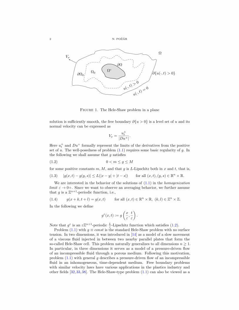
Figure 1. The Hele-Shaw problem in a plane

solution is sufficiently smooth, the free boundary ∂u > 0 is a level set of u and itsnormal velocity can be expressed as

Vν =u+t

|Du+|.

Here u+t and Du+ formally represent the limits of the derivatives from the positive

set of u. The well-posedness of problem (1.1) requires some basic regularity of g. Inthe following we shall assume that g satisfies

0 < m ≤ g ≤M(1.2)

for some positive constants m,M , and that g is L-Lipschitz both in x and t, that is,

|g(x, t)− g(y, s)| ≤ L(|x− y|+ |t− s|) for all (x, t), (y, s) ∈ Rn × R.(1.3)

We are interested in the behavior of the solutions of (1.1) in the homogenizationlimit ε→ 0+. Since we want to observe an averaging behavior, we further assumethat g is a Zn+1-periodic function, i.e.,

g(x+ k, t+ l) = g(x, t) for all (x, t) ∈ Rn × R, (k, l) ∈ Zn × Z.(1.4)

In the following we define

gε(x, t) := g

(x

ε,t

ε

).

Note that gε is an εZn+1-periodic Lε -Lipschitz function which satisfies (1.2).

Problem (1.1) with g ≡ const is the standard Hele-Shaw problem with no surfacetension. In two dimensions, it was introduced in [14] as a model of a slow movementof a viscous fluid injected in between two nearby parallel plates that form theso-called Hele-Shaw cell. This problem naturally generalizes to all dimensions n ≥ 1.In particular, in three dimensions it serves as a model of a pressure-driven flowof an incompressible fluid through a porous medium. Following this motivation,problem (1.1) with general g describes a pressure-driven flow of an incompressiblefluid in an inhomogeneous, time-dependent medium. Free boundary problemswith similar velocity laws have various applications in the plastics industry andother fields [32,33,38]. The Hele-Shaw-type problem (1.1) can also be viewed as a

HOMOGENIZATION OF THE HELE-SHAW PROBLEM 3

quasi-stationary limit of the one-phase Stefan problem with a latent heat of phasetransition depending on position and time [1, 28,31,35].

Homogenization overview. There is a large amount of literature on homogeniza-tion which is beyond the scope of this discussion and thus we refer the reader to[17,39] and the references therein.

In the context of viscosity solutions for fully nonlinear problems of the first andsecond order, the now standard approach to homogenization using correctors thatare the solutions of an appropriate cell problem was pioneered by Lions, Papanicolau& Varadhan [27] for first order equations, and later by Evans [13] for second orderequations. Unfortunately, this approach does not apply to problems like (1.1)because the zero level of solutions has a special significance and the perturbation ofa test function by a global periodic solution of some cell problem, i.e., the corrector,does not seem feasible.

The idea of using obstacle problems to recover the homogenized operator withoutthe need for a cell problem was developed by Caffarelli, Souganidis & Wang [8]for the stochastic homogenization of fully-nonlinear second order elliptic equations.It was then applied to the homogenization of the Hele-Shaw problem with spatialperiodic inhomogeneity by Kim [20], using purely the methods of the theory ofviscosity solutions. This approach was later extended to a model of contact angledynamics [21], and an algebraic rate of the convergence of free boundaries wasobtained [22].

Kim & Mellet [23, 24] later succeeded at applying a combination of viscosity andvariational approaches and obtained a homogenization result in the setting of spatialstationary ergodic random media. A related question of long-time asymptotics ofthe spatially inhomogeneous Hele-Shaw problem was addressed by the author [30].This technique relies on the special structure of problem (1.1) with time-independentg which allows us to rewrite the problem as a variational inequality of a certainobstacle problem. We refer the reader to [34] and the references therein for anexposition of obstacle problems and their homogenization.

The homogenization results for spatial media do not necessarily translate directlyto the spatiotemporal homogenization. In the context of Hamilton-Jacobi equations,for instance, a lack of uniform estimates in the spatiotemporal case was encounteredby Schwab [36] who proved the homogenization in spatiotemporal stationary ergodicrandom media, which was before established by Souganidis [37] for spatial randommedia. The situation seems to be more extreme in the case of the Hele-Shaw problemsince the homogenization in spatiotemporal media is qualitatively different even inthe periodic case.

This difference can be already observed in the homogenization of a single ordinarydifferential equation of the type x′ε(t) = f(xε(t)/ε, t/ε, xε(t)). In fact, the Hele-Shawproblem (1.1) reduces to this type of ODE in one dimension; see Section 3.1 forfurther discussion. It is known that, under some assumptions on f , xε ⇒ x locallyuniformly, where x is the solution of a homogenized ODE [15, 29]. However, theform of the homogenized problem depends on f . If, for illustration, f(y, s, x) = f(y)is a Z-periodic Lipschitz function, then the homogenized problem has the formx′(t) = f where f is the constant

(1.5) f =

(∫ 1

0

(f(y))−1 dy

)−1

.

4 N. POZAR

On the other hand, if f(y, s, x) = f(y, s) has a nontrivial dependence on both yand s, then no such explicit formula exists and, in fact, the right-hand side of thehomogenized problem, while still a constant, can possibly attain any value in therange [min f,max f ].

Another explanation of the qualitative difference, slightly more intuitive, is theinterpretation of the Hele-Shaw problem (1.1) as the quasi-stationary limit of theStefan problem. Then the quantity (g(x/ε, t/ε))−1 can be interpreted as the latentheat of phase transition, that is, the “energy” necessary to change a unit volume ofthe dry region into the wet region and advance the free boundary [30]. The “energyflux” is proportional to the gradient of the pressure. If g does not depend on time,the homogenized latent heat is simply the average, i.e.,

∫[0,1]n

(g(x))−1 dx, giving

the homogenized velocity recovered in [23] (of the form (1.5)).This formula was rigorously justified in [23] using the variational formulation via

an obstacle problem, which allows one to solve for the shape of the wet region at agiven time without the need to solve the problem at previous times. The variationalformulation was introduced in [12] using a transformation due to [3]. In a sense,for the evolution overall, the free boundary feels the same influence of the mediumno matter how it passes through it. Or, in other words, the amount of the energyrequired to fill a given region is always the same.

This drastically changes when the latent heat depends on both space and time.In this case, the energy required to advance the boundary depends on the specifichistory of the motion of the free boundary through the space-time. The varia-tional formulation does not apply anymore. What is more, it is no longer obviousthat the problem should homogenize. As the one-dimensional situation indicates—Section 3.1—the homogenized velocity might have a complicated dependence on thegradient, with velocity pinning and directional dependence. Some of these featuresappear in the spatial homogenization of non-monotone problems [21,22].

Our approach can be characterized as geometric, relying on maximum principlearguments. A similar approach to homogenization, albeit of (local) geometricmotions, was recently pursued by Caffarelli & Monneau [6]. The geometric approachto the Hele-Shaw problem is complicated by the nonlocal nature of the problem.Indeed, (1.1) can be interpreted as a geometric motion of the free boundary withthe velocity given by a nonlocal operator based on the Dirichlet-to-Neumann map.Thus the domain is of crucial importance.

Main results. We present new well-posedness and homogenization results for theHele-Shaw-type problem (1.1).

The well-posedness result is a generalization and an improvement of the previousresults in [18,20]. In full generality, we consider the Hele-Shaw type problem

−∆u(x, t) = 0 in u > 0 ∩Q,u+t (x, t) = f(x, t,Du) |Du+(x, t)|2 on ∂u > 0 ∩Q.

(1.6)

Let us introduce a number of assumptions on the function f(x, t, p) : Q× Rn → R.In the following, we use the semi-continuous envelopes f∗ and f∗ of f on Q×Rn (see(2.1) for definition). Let us point out that we do not require continuity of f(x, t, p)in p. We shall need this generality to handle the homogenized problem.

(A1) (non-degeneracy) There exist constants m and M such that 0 < m ≤f(x, t, p) ≤M for all (x, t, p) ∈ Q× Rn.


(A2) (Lipschitz continuity) There exists a constant L > 0 such that f is L-Lipschitzin x and t for all p.

(A3) (monotonicity) f∗(x, t, a1p) |a1p| ≤ f∗(x, t, a2p) |a2p| for any (x, t, p) ∈ Q×Rnand 0 < a1 < a2.

The assumption (A3) implies that the free boundary velocity is monotone withrespect to the gradient, while allowing for certain jumps.

We have the following well-posedness theorem for viscosity solutions that areintroduced in Section 2.

Theorem 1.1 (Well-posedness). Let Q := Ω × (0, T ] where Ω is a domain thatsatisfies the assumptions above and T > 0. Assume that either f(x, t, p) = f(x, t)or f(x, t, p) = f(p) and that f satisfies (A1)–(A3). Then for any positive functionψ ∈ C(∂Ω × [0, T ]) strictly increasing in time, and for any open set Ω0 ⊂ Rnwith smooth boundary, ∂Ω0 ∈ C1,1, such that Ωc ⊂ Ω0 and Ω0 ∩ Ω is bounded(see Figure 1), there exists a unique bounded viscosity solution u : Q → [0,∞) ofthe Hele-Shaw-type problem (1.6) such that u∗ = u∗ = u on ∂PQ := Q \ Q withboundary data u(x, t) = ψ(x, t) on ∂Ω× [0, T ] and initial data u(·, 0) > 0 in Ω ∩ Ω0

and u(·, 0) = 0 in Ω \ Ω0. The solution is unique in the sense that u∗ = v∗ andu∗ = v∗ for any two viscosity solutions u, v with the given boundary data.

In the context of a flow in porous media, Ωc represents the source of a liquidwith the prescribed pressure ψ on its boundary, and Ω0 is the initial wet region.The situation is depicted in Figure 1.

However, the main result of this paper concerns the homogenization of (1.1).Note that because the solution of the homogenized problem might be discontinuous,we cannot expect uniform convergence of solutions in general. Furthermore, we donot know if the homogenized velocity (r in Theorem 1.2 below) is continuous.

Theorem 1.2 (Homogenization). Suppose that g ∈ C(Rn×R) satisfies (1.2)–(1.4).Then there exists a function r : Rn → R such that

f(x, t, p) :=r(p)

|p|satisfies (A1)–(A3), and, for any Q and initial and boundary data Ω0, ψ that satisfythe assumptions in Theorem 1.1 the following results hold:

(a) the unique solutions uε of (1.1) with data Ω0, ψ converge in the sense ofhalf-relaxed limits as ε→ 0 (Definition 4.2) to the unique solution u of (1.6)with f(x, t, p) = r(p)/ |p| and the same data Ω0, ψ;

(b) if u is also continuous on a compact set K ⊂ Q then uε ⇒ u convergeuniformly on K;

(c) the free boundaries ∂(uε)∗ > 0 converge uniformly to the free boundary∂u∗ > 0 with respect to the Hausdorff distance (Definition 4.3).

Sketch of the proof. Let us give an overview of the main ideas in the paper.Since the variational formulation via an obstacle problem, discussed above, is notavailable, we have to rely solely on the technically heavy tools of the viscosity theory.The time-dependence of g poses significant new challenges which require a rathernontrivial extension of the previous results.

The first step is the identification of the homogenized problem. Since the solutionsof (1.1) are harmonic in space in their positive sets on any scale ε, their limit as ε→ 0

6 N. POZAR

should also be harmonic in space. The free boundary velocity of the homogenizedproblem is, however, unknown. Following the ideas from [8, 20], we identify thecorrect homogenized free boundary velocity by solving an obstacle problem andstudy its behavior as ε→ 0. To motivate our approach, suppose that the solutionsuε in the limit ε→ 0 converge to a solution u of the homogenized Hele-Shaw problemwith the free boundary law given as

Vν = r(Du) on ∂u > 0,

where a 7→ r(aq) is an increasing function on R+ for any q ∈ Rn. The crucialobservation is that this problem has traveling wave solutions; these are the planarsolutions of the form Pq,r(x, t) = (|q| rt+x · q)+, with the particular choice r = r(q).Here (·)+ stands for the positive part, i.e., s+ := max(s, 0). If r > r(q) then Pq,r is asupersolution of the homogenized problem, and if r < r(q) it is a subsolution. Thisobservation allows us to identify the correct velocity r(q) by solving the ε-problem(1.1) for each ε > 0 and comparing the solution with the planar solution Pq,r forgiven r and q. Loosely speaking, if r is too large for a given q, the solutions uε

should evolve slower than Pq,r for small ε and, similarly, if r is too small then uε

should evolve faster than Pq,r for small ε.To make this idea rigorous, we solve the following obstacle problems for each

fixed ε: given a fixed domain Q, r and q, find the largest subsolution uε;q,r ofthe ε-problem that stays under Pq,r in Q and the smallest supersolution uε;q,r ofthe ε-problem that stays above Pq,r in Q. Following this reasoning, we find twocandidates for the correct homogenized velocity r(q) by “properly measuring” howmuch contact there is as ε→ 0 between the obstacle Pq,r and the largest subsolutionuε;q,r, yielding r(q), and the smallest supersolution uε;q,r, yielding r(q). Since thefree boundary velocity law is nonlocal, given by a Dirichlet-to-Neumann map, agood choice of the domain Q for this procedure is important.

For homogenization to occur, it is necessary that both candidates r(q) and r(q)yield the same limit problem (1.6). We need to give a proper meaning to the intuitiveidea of evolving slower or faster than the obstacle Pq,r. The selection of a quantitythat not only “properly measures” the amount of contact between the obstacle Pq,rand the solutions of the obstacle problem in the homogenization limit ε → 0 butis also convenient to work with is far from obvious. In particular, we want to takeadvantage of the natural monotonicity (Birkhoff property) of the solutions of theobstacle problem, which is a consequence of the periodicity of the medium.

In [8] as well as in [20–22], the authors consider the coincidence set of the solutionsof the obstacle problem and the obstacle Pq,r as their quantity of choice. This choiceis motivated by the fact that if there is a contact on a sufficiently large set, thenthe solution must be close to the obstacle everywhere. This kind of estimate canbe established using the Alexandroff-Bakelman-Pucci estimate in the case of fullynonlinear elliptic problems in [8]. Since ABP-type estimates are not available for theHele-Shaw problem, the closeness to the obstacle must be derived by other means[20].

The disadvantage of this approach in the context of free boundary problems,in particular for the homogenization of (1.1), stems from the restriction that itimposes on the directions in which one can translate the solutions of the obstacleproblem to take advantage of their natural monotonicity property, and to recoverthe monotonicity of the contact set. This creates technical difficulties and requires aseparate treatment of rational and irrational directions. It seems that, to overcome


these difficulties, it is necessary to scale the solutions in time for the arguments towork. However, a scaling in time is not available in the time-dependent medium.

The main new idea in this paper is the introduction of flatness and its critical valueεβ (Section 3.4). More specifically, to recover the correct homogenized boundaryvelocity for a given gradient q we test if, for some fixed β ∈ (0, 1), the free boundaryof the solution of the obstacle problem stays εβ-close to the obstacle for a unit timeon an arbitrary small scale ε. This choice is motivated by the new cone flatnessproperty (Proposition 3.20): the boundary of the solution of the obstacle problem

stays between two cones that are ∼ ε |ln ε|1/2 apart. Therefore if, for ε 1, the

boundary is farther than εβ ε |ln ε|1/2, it will be detached from the obstacle on alarge set. This is formulated in the detachment lemma (Lemma 3.23). Moreover, theimprovement of the local comparison principle (Theorem 3.16) for εβ-flat solutionsto allow for β ∈ (4/5, 1) is a necessary ingredient to close the argument. Thisapproach allows us to prove that the candidates r(q) and r(q) almost coincide, i.e.,r = r∗, and that f(x, t, p) = r(p)/ |p| satisfies the assumptions (A1)–(A3). Moreover,if the medium is time-independent, that is, g(x, t) = g(x), we are able to show thatr = r are continuous and one-homogeneous (Section 3.10), essentially recovering theresult of [20].

Once the homogenized velocity has been identified, we can prove that the half-relaxed limits satisfy the homogenized problem (Section 4). The perturbed testfunction method cannot be applied to free boundary problems and a different, moregeometric argument based on a comparison of the solutions of the ε-problem withrescaled translations of the solutions of the obstacle problems must be engaged. Thedetachment lemma (Lemma 3.23) plays a key role in this argument. Finally, sincethe comparison with barriers guarantees that the limits have the correct boundarydata, the comparison principle for the limit problem establishes that the upperand lower half-relaxed limits coincide with the unique solution of the homogenizedproblem.

Open problems. Let us conclude the introduction by mentioning some of theopen problems. We have been only able to show that the homogenized velocity r issemi-continuous. However, it seems quite reasonable to expect continuity, or evenHolder continuity. As the one-dimensional case suggests in Section 3.1, this is thehighest regularity one may hope for in a general situation. Another open problem isthe question of a convergence rate of free boundaries in the homogenization limit.An algebraic rate was obtained in the periodic spatial homogenization case [22].These issues will be addressed in future work.

A related open problem is the homogenization in random media when the freeboundary problem does not have a variational structure, unlike [23,24]. This problemhas not yet been solved since there is no obvious subadditive quantity to which thesubadditive ergodic theorem can be applied to overcome the lack of compactness ofa general probability space.

Finally, in the current paper, we use the monotone propagation property of thefree boundary—that is, that the wet region cannot recede—to obtain some of theimportant estimates. The presented method, however, seems robust enough tohandle non-monotone problems such as the model of contact angle dynamics as in[21,22]. This will also be a subject of future work.

8 N. POZAR

Outline. The exposition of the proof of the homogenization result was split in anumber of steps. First we give the necessary definitions of solutions in Section 2,together with some preliminary results including the comparison principle and awell-posedness result. These are used in Section 3, where we identify a candidatefor the limit velocity. Finally, Section 4 is devoted to showing that the solutionsconverge in the homogenization limit. In addition, the appendices contain someauxiliary results used throughout the text.

2. Viscosity solutions

In this section, we briefly revisit the theory of viscosity solutions of the Hele-Shawproblem (1.1). We generalize the definitions introduced in [18, 20], and outlinethe proof of the comparison principle in our settings, Section 2.1, with an aim atestablishing Theorem 1.1 in Section 2.2. Let us mention that viscosity solutionsseem to be the natural class of solutions of (1.1) since the problem has a maximumprinciple structure. Moreover, due to the possible topological changes and mergingof free boundaries, the solutions might be discontinuous [18]. The standard notionof solutions due to [12] does not apply when g in (1.1) depends on time.

Since viscosity solutions are the only weak notion of solutions used throughoutthe paper, we will often refer to them simply as solutions.

Before we give the definitions of viscosity solutions, we need to introduce somenotation. For given radius ρ > 0 and center (x, t) ∈ Rn × R, we define the openballs

Bρ(x, t) :=

(y, s) ∈ Rn × R : |y − x|2 + |s− t|2 < ρ2,

Bρ(x) := y ∈ Rn : |y − x| < ρ.

Let E ⊂ Rd for some d ≥ 1. Then USC(E) and LSC(E) are respectively the sets ofall upper semi-continuous and lower semi-continuous functions on E. For a locallybounded function u on E we define the semi-continuous envelopes u∗,E ∈ USC(Rd)and u∗,E ∈ LSC(Rd) as

u∗,E := infv ∈ USC(Rd) : v ≥ u on E

,

u∗,E := supv ∈ LSC(Rd) : v ≤ u on E

.

(2.1)

Note that u∗,E : Rd → [−∞,∞) and u∗,E : Rd → (−∞,∞] are finite on E. Wesimply write u∗ and u∗ if the set E is understood from the context. The envelopescan be also expressed as

u∗,E(x) = limδ→0

sup u(y) : y ∈ E, |y − x| < δ for x ∈ E, u∗,E = −(−u)∗,E .

It will be also useful to use a shorthand notation for the set of positive values ofa given function u : E → [0,∞), defined on a set E ⊂ Rn × R,

Ω(u;E) := (x, t) ∈ E : u(x, t) > 0, Ωc(u;E) := (x, t) ∈ E : u(x, t) = 0,

and the closure Ω(u;E) := Ω(u;E). For t ∈ R, the time-slices Ωt(u;E), Ωt(u;E)and Ωct(u;E) are defined in the obvious way, i.e.,

Ωt(u;E) =x : (x, t) ∈ Ω(u;E)

, etc.


We shall call the boundary of the positive set in E the free boundary of u and denoteit Γ(u;E), i.e.,

Γ(u;E) = (∂Ω(u;E)) ∩ E.

If the set E is understood from the context, we shall simply write Ω(u), etc.For given constant τ ∈ R we will often abbreviate

t ≤ τ := (x, t) ∈ Rn × R : t ≤ τ, etc.

It will be convenient to define viscosity solutions on general parabolic neighbor-hoods; we refer the reader to [40] for a more general definition.

Definition 2.1 (Parabolic neighborhood and boundary).A nonempty set E ⊂ Rn ×R is called a parabolic neighborhood if E = U ∩ t ≤ τfor some open set U ⊂ Rn × R and some τ ∈ R. We say that E is a parabolicneighborhood of (x, t) ∈ Rn × R if (x, t) ∈ E. Let us define ∂PE := E \ E, theparabolic boundary of E.

Remark 2.2. Since intE = U ∩ t < τ, one can observe that ∂PE = ∂E \ (U ∩ t = τ).If E = U then ∂PE = ∂E. Note that we do not require that E 6= U , which is usuallyassumed, simply because it is unnecessary in this paper. Adding this requirement does notchange any of the results presented.

Following [18, 20], we define the viscosity solutions for (1.6). In the followingdefinitions, Q ⊂ Rn × R is an arbitrary parabolic neighborhood in the sense ofDefinition 2.1 and f(x, t, p) : Q×Rn → R satisfies assumptions (A1)–(A3) (Section 1).We do not assume that f is continuous in p.

Definition 2.3. We say that a locally bounded, non-negative function u : Q→ [0,∞)is a viscosity subsolution of (1.6) on Q if

(i) (continuous expansion)

Ω(u;Q) ∩Q ∩ t ≤ τ ⊂ Ω(u;Q) ∩ t < τ for every τ > 0,

(ii) (maximum principle)for any φ ∈ C2,1 such that u∗ − φ has a local maximum at (x0, t0) ∈Q ∩ Ω(u;Q) in Ω(u;Q) ∩ t ≤ t0, we have(ii-1) if u∗(x0, t0) > 0 then −∆φ(x0, t0) ≤ 0,(ii-2) if u∗(x0, t0) = 0 then either −∆φ(x0, t0) ≤ 0 or Dφ(x0, t0) = 0

or [φt − f∗(x0, t0, Dφ(x0, t0)) |Dφ|2](x0, t0) ≤ 0.

Remark 2.4. The condition (i) in Definition 2.3 is necessary to prevent a scenario wherea ‘bubble’ closes instantly; more precisely, a subsolution cannot become instantly positiveon an open set surrounded by a positive phase, or cannot fill the whole space instantly.

The definition of a viscosity supersolution is similar.

Definition 2.5. We say that a locally bounded, non-negative function u : Q→ [0,∞)is a viscosity supersolution of (1.6) on Q if

(i) (monotonicity of support)if (ξ, τ) ∈ Ω(u∗;Q) then (ξ, t) ∈ Ω(u∗;Q) for all (ξ, t) ∈ Q, t ≥ τ .

(ii) (maximum principle)for any φ ∈ C2,1 such that u∗ − φ has a local minimum at (x0, t0) ∈ Q int ≤ t0, we have(ii-1) if u∗(x0, t0) > 0 then −∆φ(x0, t0) ≥ 0,

10 N. POZAR

(ii-2) if u∗(x0, t0) = 0 then either −∆φ(x0, t0) ≥ 0 or Dφ(x0, t0) = 0

or [φt − f∗(x0, t0, Dφ(x0, t0)) |Dφ|2](x0, t0) ≥ 0.

Remark 2.6. The condition (i) in Definition 2.5 states that the support of a supersolutionis nondecreasing. It is a purely technical assumption which simplifies the proof of thecomparison theorem by preventing an instantaneous disappearance of a component of apositive phase. Indeed, it can be shown that all solutions of the Hele-Shaw problem havenondecreasing support. This assumption can be removed by using the tools developed in[26].

Finally, we define a viscosity solution by combining the two previous definitions.

Definition 2.7. A function u : Q→ [0,∞) is a viscosity solution of (1.6) on Q ifu is both a viscosity subsolution and a viscosity supersolution on Q.

It will be useful to state an equivalent definition of viscosity solutions via a com-parison with barriers, which in our case are strict classical sub- and supersolutions.This definition seems more natural, as it follows a more common pattern appearingin the treatment of free boundary problems; see [2, 4, 7, 9, 25,26].

Definition 2.8. For a given closed set K ∈ Rn × R, we say that φ ∈ C2,1x,t (K) if

there exists open set U ⊃ K and ψ ∈ C2,1x,t (U), i.e., a function twice continuously

differentiable in space and once in time, such that φ = ψ on K.

Definition 2.9. Given a nonempty open set U ⊂ Rn × R, a function φ ∈ C(U) ∩C2,1x,t (Ω(φ;U)) is called a subbarrier of (1.6) in U if there exists a positive constant

c such that

(i) −∆φ < −c on Ω(φ;U), and

(ii) |Dφ+| > c and φ+t − f∗(·, ·, Dφ+) |Dφ+|2 < −c on Γ(φ;U).

Here Dφ+ and φ+t denote the limits of Dφ and φt, respectively, on Γ(φ;U) from

Ω(φ;U).

Definition 2.10. Given a nonempty open set U ⊂ Rn ×R, a function φ ∈ C(U) ∩C2,1x,t (Ω(φ;U)) is called a superbarrier of (1.6) in U if there exists a positive constant

c such that

(i) −∆φ > c on Ω(φ;U), and

(ii) |Dφ+| > c and φ+t − f∗(·, ·, Dφ+) |Dφ+|2 > c on Γ(φ;U).

A notion of strict separation is a crucial concept in the theory and will be usedmultiple times (our definition differs slightly from the one introduced in [18]).

Definition 2.11 (Strict separation). Let E ⊂ Rn × R be a parabolic neighborhood,and u, v : E → R be bounded non-negative functions on E, and let K ⊂ E. We saythat u and v are strictly separated on K with respect to E, and we write u ≺ v inK w.r.t. E, if

u∗,E < v∗,E in K ∩ Ω(u;E).

A definition of viscosity solutions using barriers follows.

Definition 2.12. We say that a locally bounded, non-negative function u : Q →[0,∞) is a viscosity subsolution of (1.6) on Q if for every bounded parabolicneighborhood E = U ∩ t ≤ τ, E ⊂ Q, and every superbarrier φ on U such thatu ≺ φ on ∂PE w.r.t. E, we also have u ≺ φ on E w.r.t. E.


Similarly, a locally bounded, non-negative function u : Q→ [0,∞) is a viscositysupersolution if Definition 2.5(i) holds and for any subbarrier φ on U such thatφ ≺ u on ∂PE w.r.t. E, we also have φ ≺ u on E w.r.t. E.

Finally, u is a viscosity solution if it is both a viscosity subsolution and a viscositysupersolution.

We finish this section by stating the equivalence of the two definitions of viscositysolutions.

Proposition 2.13. The definitions of viscosity subsolutions (resp. supersolutions)in Definition 2.3 (resp. 2.5) and in Definition 2.12 are equivalent.

Before proceeding with the proof, let us state a useful property of a strictseparation on time dependent sets.

Lemma 2.14. Suppose that E is a bounded parabolic neighborhood and u, v arenon-negative locally bounded functions on E. The set

Θu,v;E :=τ : u ≺ v in E ∩ t ≤ τ w.r.t. E

(2.2)

is open and Θu,v;E = (−∞, T ) for some T ∈ (−∞,∞].

Proof. By replacing u by u∗,E and v by v∗,E , we may assume that u is uppersemi-continuous and v is lower semi-continuous. Let us choose τ ∈ Θu,v;E . Clearlys ∈ Θu,v;E for all s ≤ τ . Therefore, we only need to show that there exists s > τ such

that s ∈ Θu,v;E . We can assume that t ≤ τ ∩E 6= ∅, otherwise the claim is trivial

since E is compact. Suppose that u 6≺ v on E∩t ≤ s w.r.t. E for all s > τ . Hencethere is a sequence (xk, tk) ∈ Ω(u;E) such that tk τ and u(xk, tk) ≥ v(xk, tk).By compactness of E, we can assume that (xk, tk) → (ξ, τ), and we see that(ξ, τ) ∈ Ω(u;E) ∩ t ≤ τ. By semi-continuity we have u(ξ, τ) − v(ξ, τ) ≥ 0, acontradiction with u ≺ v in E ∩ t ≤ τ.

Proof of Proposition 2.13. Let us prove the statement for subsolutions. Supposethat u is a subsolution on some parabolic neighborhood Q in the sense of Defini-tion 2.3. By taking the semi-continuous envelope, we can assume that u ∈ USC(Q).

Let E = U ∩ t ≤ τ ⊂ Q be a bounded parabolic neighborhood and let φ bea superbarrier on U such that u ≺ φ on ∂PE w.r.t. E. Consider the set Θu,φ,E ,

introduced in (2.2). Let us define t = sup Θu,φ,E . Since E is bounded, we have

t > −∞. To show that u is a subsolution in the sense of Definition 2.12, it is enoughto show that u ≺ φ in E, which is equivalent to t = +∞.

Hence suppose that t < +∞. Lemma 2.14 implies that(a) u 6≺ φ in E ∩

t ≤ t

w.r.t. E,

(b) u ≺ φ in E ∩ t ≤ s for all s < t, and, finally,(c) Ω(u;E) ∩

t ≤ t

⊂ Ω(φ;E) due to (b) and the continuous expansion in Defini-

tion 2.3(i).By semi-continuity and compactness, u− φ has a local maximum at some point

(ξ, σ) in Ω(u;E)∩t ≤ t

. Then (a) implies that u(ξ, σ)−φ(ξ, σ) ≥ 0. Consequently,

since (b) holds, we must have σ = t, and u ≺ φ on ∂PE implies (ξ, t) ∈ E. Finally,using (c) we conclude that (ξ, t) ∈ E ∩ Ω(u;E) ∩ Ω(φ;E). Therefore either:

• u(ξ, t) > 0, and that is a contradiction with Definition 2.3(ii-1); or• u(ξ, t) = 0, but then φ(ξ, t) = 0 and consequently (ξ, t) ∈ Γ(φ;E), which

yields a contradiction with Definition 2.3(ii-2).

12 N. POZAR

The proof for supersolutions is analogous, but more straightforward since thesupport of u∗ cannot decrease due to Definition 2.5(i).

The direction from Definition 2.12 to Definitions 2.3 and 2.5 is quite standard.In particular, Definition 2.3(i) can be shown by a comparison with barriers asin the proof of Corollary A.6. Furthermore, any test function φ such that u − φhas a local maximum at (x, t) and violates either of Definition 2.3(ii) can beused for a construction of a superbarrier in a parabolic neighborhood of (x, t) by

considering φ(x, t) = (φ(x, t) + |x− x|4 + |t− t|2 − φ(x, t))+. Once again, the prooffor supersolutions is similar.

Definition 2.15. For a given function f and a nonempty parabolic neighborhoodQ ⊂ Rn × R, we define the following classes of functions:

• S(f,Q), the set of all viscosity supersolutions of the Hele-Shaw problem (1.6)on Q;• S(f,Q), the set of all viscosity subsolutions of (1.6) on Q;• S(f,Q) = S(f,Q) ∩ S(f,Q), the set of all viscosity solutions of (1.6) on Q.

We have the following obvious inclusions:

Lemma 2.16. Let Q ⊂ Rn×R be a nonempty parabolic neighborhood. If f ≤ g forgiven functions f, g : Q× Rn → (0,∞) then

S(f,Q) ⊃ S(g,Q) and S(f,Q) ⊂ S(g,Q).

Finally, we observe that subsolutions and supersolutions can be “stitched” to-gether.

Lemma 2.17. Let Q1, Q2 ⊂ Rn × R be two parabolic neighborhoods such thatQ1 ⊂ Q2 and let ui ∈ S(f,Qi), i = 1, 2, for some f(x, t, p) : Q2×Rn → (0,∞). Wedefine

u =

max(u1, u2) in Q1,

u2 in Q2 \Q1.

If u∗,Q1

1 ≤ u∗,Q2

2 on (∂PQ1) ∩Q2 and

(2.3) Ω(u1;Q1) ∩ ∂PQ1 ⊂ Ω(u2;Q2)

then u ∈ S(f,Q2).Let now vi ∈ S(f,Qi), i = 1, 2, and we define

v =

min(v1, v2) in Q1,

v2 in Q2 \Q1.

If (v1)∗,Q1≥ (v2)∗,Q2

on (∂PQ1) ∩Q2, then v ∈ S(f,Q1).

Proof. Let us show the proof for subsolutions. We use Definition 2.3. ClearlyΩ(u;Q2) = Ω(u1;Q1) ∪ Ω(u2;Q2) and therefore, by (2.3), we have

Ω(u;Q2) = Ω(u1;Q1) ∪ Ω(u2;Q2)

= (Ω(u1;Q1) ∩Q1) ∪ (Ω(u1;Q1) ∩ ∂PQ1) ∪ Ω(u2;Q2)

= (Ω(u1;Q1) ∩Q1) ∪ Ω(u2;Q2).


Thus Definition 2.3(i) is clear. To prove (ii), suppose that u∗ − φ has a localmaximum at (x, t) ∈ Ω(u;Q2) in Ω(u;Q2)∩

t ≤ t

. We observe that, by hypothesis,

u∗ = max(u∗,Q1

1 , u∗,Q2

2 ) on Q1 and u∗ = u∗,Q2

2 on Q2 \ Q1. Consequently, if(x, t) ∈ Q1 then u∗1 − φ and/or u∗2 − φ have a local maximum in the appropriate set,and if (x, t) ∈ Q2 \Q1 then u∗2 − φ has a local maximum. Definition 2.3(ii) followsfrom this observation.

The proof for supersolutions is straightforward since there is no restriction ontheir supports.

2.1. Comparison principle. A crucial result for a successful theory of viscositysolutions is a comparison principle. In this section we establish the comparisonprinciple between strictly separated viscosity solutions on an arbitrary parabolicneighborhood. We only give an outline of the proof and point out the differencesfrom previous results in [18,20,26].

Theorem 2.18. Let Q be a bounded parabolic neighborhood. Suppose that f :Q × Rn → R is a given function that satisfies the assumptions (A1)–(A3) andis of the form either f(x, t, p) = g(x, t) or f(x, t, p) = f(p). If u ∈ S(f,Q) andv ∈ S(f,Q) such that u ≺ v on ∂PQ w.r.t. Q, then u ≺ v in Q w.r.t. Q.

Proof. Step 1. We can assume that u ∈ USC(Q) and v ∈ LSC(Q). Similarly to theproof of Proposition 2.13, we consider the set Θu,v;Q, defined in (2.2), and introduce

t0 := sup Θu,v;Q > −∞. Then u ≺ v on Q w.r.t. Q is equivalent to t0 = +∞.

Therefore suppose that t0 < +∞. Let us introduce the sup- and inf-convolutions

Z(x, t) =

(1 +

3Lr

m

)sup

Ξr(x,t)

u,

W (x, t) =

(1− 3Lr

m

)inf

Ξr−δt(x,t)v(x, t),

with 0 < r m3L and δ = r

2T where T := inf τ : Q ⊂ t ≤ τ. The open setΞr(x, t) is defined as

Ξr(x, t) =

(y, s) : (|y − x| − r)2+ + |s− t|2 < r2

.

We refer the reader to [18,26] for a detailed discussion of the properties of Z and W .In particular, Z and W are well-defined on the closure of the parabolic neighborhoodQr,

Qr :=

(x, t) : Ξr(x, t) ⊂ Q,

and Z ∈ USC(Qr) and W ∈ LSC(Qr).Moreover, Z ∈ S(f,Qr) and W ∈ S(f,Qr). This is straightforward if f(x, t, p) =

f(p). However, if f depends on (x, t) as in f(x, t, p) = g(x, t) we have to useProposition B.1 with factors a = (1± 3Lr/m), yielding the same conclusion.

Finally, and this is the main motivation for the choice of the convolutions, bothZ and W have an important interior/exterior ball property of their level sets bothin space for each time and in space-time; see [26].

Step 2. Since u ≺ v on ∂PQ w.r.t. Q, we claim that if r is chosen small enoughwe have Z ≺W on ∂PQr w.r.t. Qr. Suppose that this is not true for any r > 0. Letrk → 0 as k →∞. There exists a sequence of (xk, tk) ∈ ∂PQrk ∩ Ω(Zrk ;Qrk) suchthat Zrk(xk, tk) ≥Wrk(xk, tk). By definition of Z and W and semi-continuity, there

14 N. POZAR

exist (ξk, σk), (ζk, τk) ∈ Ξrk(xk, tk) such that (ξk, σk) ∈ Ω(u;Q) and u(ξk, σk) ≥v(ζk, τk). By compactness of Ω(u;Q), for a subsequence, still denoted by k, (ξk, σk)converges to a point (ξ, σ), which must lie in ∂PQ ∩ Ω(u;Q). A simple observation(ζk, τk) ∈ Ξ2rk(ξk, σk) then implies that (ζk, τk) → (ξ, σ). This is a contradictionwith the semi-continuity of u and v and the fact that u(ξ, σ) < v(ξ, σ).

Step 3. We claim that W is a supersolution of (1.6) on Qr with the free boundary

velocity increased by δ, that is, with fδ(x, t, p) = f(x, t, p) + δ |p|−1. As we already

know that W ∈ S(f,Qr), we only need to verify Definition 2.5(ii-2). Thus supposethat φ is a C2,1-function and W −φ has a strict local minimum 0 at (ξ, σ) in t ≤ σ,and W (ξ, σ) = 0, −∆φ(ξ, σ) < 0 and |Dφ(ξ, σ)| > 0. By semi-continuity thereexists (y, s) ∈ Ξr−δσ(0, 0) with(

1− 3Lr

m

)v(ξ + y, σ + s) = W (ξ, σ).

Moreover, the definition of φ and W implies that

φ(x, t) ≤W (x, t) ≤(

1− 3Lr

m

)v(x+ y + z, t+ s),(2.4)

for any (y + z, s) ∈ Ξr−δt(0, 0) and (x, t) in a neighborhood of (ξ, σ), t ≤ σ. Sincethe set Ξr−δt(0, 0) is decreasing in t, we can take any z ∈ Bδ(σ−t)(0). Let us define

ν = − Dφ|Dφ| (ξ, σ), the unit outer normal to Ωσ(φ) at ξ. With the particular choice

z = −δ(σ − t)ν, we can rewrite (2.4) after a change of variables as

ψ(x, t) :=

(1− 3Lr

m

)−1

φ(x− y + δ(σ + s− t)ν, t− s) ≤ v(x, t),

for (x, t) close to (ζ, µ) := (ξ + y, σ + s), t ≤ σ + s. Additionally, the equalityholds at (ζ, µ) by the choice of (y, s). Thus ψ is a test function for v at (ζ, µ) forDefinition 2.5(ii-2), and we have

[φt − δ |Dφ|](ξ, σ) =

(1− 3Lr

m

)ψt(ζ, µ)

≥(

1− 3Lr

m

)f∗ (ζ, µ,Dψ(ζ, µ)) |Dψ(ζ, µ)|2

=

(1− 3Lr

m

)−1

f∗

(ζ, µ,

(1− 3Lr

m

)−1

Dφ(ξ, σ)

)|Dφ(ξ, σ)|2 .

If f(x, t, p) = g(x, t), then we use the assumptions (A1)–(A2) that imply g(ζ, µ) ≥(1− 3Lr

m

)g(ξ, σ), and if f(x, t, p) = f(p) we use the assumption (A3) to conclude

that

[φt − δ |Dφ|](ξ, σ) ≥ f∗(ξ, σ,Dφ(ξ, σ)) |Dφ(ξ, σ)|2 .

Therefore W ∈ S(fδ, Qr).

Step 4. We proceed with the proof of the comparison theorem. Let us set

t = sup ΘZ,W ;Qr

and observe that t ≤ t0.

As in the proof of Proposition 2.13, we have Ω(Z) ∩t ≤ t

⊂ Ω(W ) ∩

t < t

,

and there exists (ξ, t) ∈ Qr ∩ Ω(Z) ∩ Ω(W ) such that (ξ, t) is a point of maximum


of Z − W in Ω(Z) ∩t ≤ t

, and Z(ξ, t) − W (ξ, t) ≥ 0. Since the set Ωc

t(W )

has the interior ball property of radius r/2, we can show by a barrier argumentthat in fact Z = 0 on Ωc(W ) ∩

t ≤ t

, see [18, 26] for details. Most of the

arguments are analogous since Z ∈ S(M,Qr), W ∈ S(m,Qr). This together withthe assumption that Ω(W ) cannot decrease in time due to Definition 2.5(i) yieldsΩ(Z) ∩

t ≤ t

⊂ Ω(W ).

Suppose that Z(ξ, t) > 0. Let us denote by U the connected component ofΩt(W ) that contains (ξ, t). Since Z(·, t) is subharmonic in the (open) set U , Z(·, t)cannot be identically zero on ∂U . But the conclusion of the previous paragraphimplies that Z ≡ 0 on (∂U ×

t

) ∩ Qr. Hence (∂U ×t

) ∩ ∂PQr 6= ∅. Wehave 0 < Z < W at the points of ∂PQr where Z > 0 by the assumption of strictseparation. Consequently, a straightforward argument of adding a small harmonicfunction to Z, using the comparison principle for subharmonic and superharmonicfunctions, yields Z(ξ, t) < W (ξ, t), a contradiction with the previous paragraph.

Therefore Z(ξ, t) = W (ξ, t) = 0 and Z ≤ W ont ≤ t

. We arrive at the last

step of the comparison theorem, where we need to find some weak ordering ofgradients and the corresponding velocities, as in [26].

Step 5. Hopf’s lemma implies that the “gradients” of Z and W are strictlyordered. Indeed, let ν be the unique unit outer normal of Ωt(Z) and Ωt(W ) atξ. Since Z(·, t) is subharmonic in U and W is superharmonic in U , and there isan interior ball of Ωt(Z) at ξ, and W (·, t) 6≡ Z(·, t) in U , we can apply the Hopf’slemma in U at ξ ∈ ∂U and conclude that

α := lim suph→0

Z(ξ − hν, t)h

< lim infh→0

W (ξ − hν, t)h

=: β.(2.5)

The assumption on f implies

f∗(ξ, t,−αν

)|−αν| ≤ f∗

(ξ, t,−βν

)|−βν| .(2.6)

It can be showed as in [18] (see also [25, 26]) that the sets Ω(Z) and Ωc(W ) haveinterior space-time balls at (ξ, t) with space-time slopes that represent the velocitiesof the free boundaries at (ξ, t) which we denote as mZ and mW . A barrier argumentyields 0 < δ ≤ mW ≤ mZ <∞, using the result of Step 3.

Step 6. Now we proceed as in [26]: There are points (ξu, tu) and (ξv, tv) onthe free boundaries of u and v, respectively, such that (ξu, tu), (ξv, tv) ∈ ∂Ξr(ξ, t).Since Z ≤ W for t ≤ t and Z > 0 on Ξr(ξu, tu), we can deduce that v > 0 on⋃

Ξr−δt(x, t), where the union is over all points (x, t) ∈ Ξr(ξu, tu), t ≤ t. Thereforeas in [26, Lemma 3.23], given arbitrary η > 0 small we can put a radial test functionunder v in a neighborhood of (ξv, tv) that touches v from below at (ξv, tv) with free

boundary velocity mZ − δ + η and gradient −(1− 3Lr

m

)−1(β − η)ν at (ξv, tv). The

definition of supersolution then implies

mZ − δ + η ≥ f∗

(ξv, tv,−

(1− 3Lr

m

)−1

(β − η)ν

)(1− 3Lr

m

)−1

(β − η),

which can be estimated using (A1)–(A2) or (A3), depending on the form of f as inStep 3, as

≥ f∗(ξ, t,−(β − η)ν)(β − η).

16 N. POZAR

Sending η → 0, the lower semi-continuity of f∗ implies

mZ − δ ≥ f∗(ξ, t,−βν)β.

A similar, but more direct proof using the fact that Z = 0 on Ξr(ξ, t) establishes

mZ ≤ f∗(ξ, t,−αν)α.

When we combine these two inequalities through (2.6), we arrive at

mZ ≤ f∗(ξ, t,−αν

)α ≤ f∗

(ξ, t,−βν

)β ≤ mZ − δ,

a contradiction. Therefore Z and W cannot cross, which in turn implies that u andv cannot cross and hence u ≺ v in Q w.r.t. Q.

2.2. Well-posedness. We will use the comparison principle, Theorem 2.18, toestablish the well-posedness of the Hele-Shaw-type problem (1.6), Theorem 1.1.Since Theorem 2.18 requires strictly separated boundary data, it does not provideuniqueness of solutions for general boundary data. However, it is possible to proveuniqueness when the boundary data features some special structure; see [18,20]. Weshow the well-posedness theorem for boundary data strictly increasing in time.

Proof of Theorem 1.1. In this proof we return to the parabolic cylinder Q = Ω×(0, T ] introduced in Section 1.

Bounded support. First observe that exactly one of Ω and Ω0 is bounded and thatboth ∂Ω and ∂Ω0 are bounded.

Let u be a bounded viscosity solution on Q with the correct boundary data. Wewill show that Ω(u;Q) ⊂ BR(0)× [0, T ] for some large R. If Ω is bounded, this isobvious. Therefore assume that Ω is unbounded and therefore Ω0 is bounded. Letd = diam Ω0 > 0, set K := supQ u <∞ (by assumption) and recall that M is the

upper bound on f . We define µ := 2√

2nKMT and R := d + µ. The claim nowfollows from Corollary A.6 applied with E = Ω0

c. We set Σ := BR(0) ∩ Ω, which is

clearly bounded. Note that ∂Ω0 ⊂ BR(0).

Barriers. Before proceeding with the proof of existence, let us first construct barriersfor the Perron’s method. We write Ωρ

0 := Ω0 + Bρ(0), Ω00 := Ω0. Since ∂Ω0 is

C1,1 and compact, it is a set of a positive reach and there exists ρ0 > 0 such that∂Ωρ0 ∈ C1,1 and ∂Ωρ0 ⊂ BR(0) for ρ ∈ [0, ρ0].

For ρ ∈ [0, ρ0], t ∈ [0, T ], let us define uρt ∈ C(Ω), such that ∆uρt = 0 in Ωρ0 ∩ Ω

with boundary data uρt (x) = ψ(x, t) on ∂Ω, uρt = 0 in Ω \ Ωρ0.Since ∂Ω ⊂ BR(0) and ∂Ω ∈ C0,1, we can extend ψ to C(Rn×[0, T ]) as ∆ψ = 0 in

(BR(0)\∂Ω)× [0, T ] and ψ = 0 in BcR(0)× [0, T ]. Observe that ψ ∈ S(M,Σ× [0, T ]).Now we introduce the barriers at the initial time t = 0. By the Hopf’s lemma

and comparison for harmonic functions, and the fact that ψ is bounded fromabove and from zero on ∂Ω × [0, T ], there exists a constant c > 0 such that0 < c−1 ≤ |D(uρt )

+| ≤ c on ∂Ωρ0 for all ρ ∈ [0, ρ0/2], t ∈ [0, T ]. Therefore

we can find ω > 0 large enough so that U(x, t) := uω−1tt (x) is a subsolution

U ∈ S(m/2,Ω× (0, δ]), and V (x, t) := uωtt (x) is a supersolution V ∈ S(M,Ω× (0, δ])for some δ ∈ (0, ρ0/ω). Moreover, U, V ∈ C(Ω× [0, δ]). Let us extend U and V by

defining U(x, t) = uω−1δt (x) and V (x, t) = ψ(x, t) for t ∈ (δ, T ] (recall the extension

of ψ above). It is straightforward to show that U ∈ S(m/2, Q), V ∈ S(M,Q) andthat U and V satisfy the boundary condition on ∂PQ in the correct sense. That is,U∗ = U∗ = V ∗ = V∗ = ψ on ∂Ω× [0, T ] and U∗ = U∗ = V ∗ = V∗ = u0

0.


Uniqueness. Let u and v be two solutions with the correct boundary data.We first check the value of u and v at t = 0. In general, for any solution u, we

have u∗(·, t) is subharmonic in Ω and u∗(·, t) is superharmonic in Ωt(u∗;Q) (see [26]for a detailed proof). Thus a simple argument, using the facts that a support of asubsolution must expand continuously, and that a support of a supersolution cannotdecrease, shows that u∗(·, 0) = u∗(·, 0) = v∗(·, 0) = v∗(·, 0) = u0

0 on Ω.Now we observe that the support of a supersolution u is strictly increasing at

t = 0, i.e., Ω0(u∗;Q) = Ω ∩ Ω0 ⊂ Ωt(u∗;Q) for any t > 0. This follows from thecomparison with a perturbation of U . Specifically, fix a point ζ ∈ BR(0) \ Ω and

define Uκ(x, t) = (U(x, t) + κ |x− ζ|2 − 4κR2)+. Clearly Uκ ⇒ U uniformly on Qas κ→ 0 and Uκ is a subbarrier on Ω× (0, δ] for κ > 0 small enough (recall thatU ∈ S(m/2, Q) with m/2 < m). Moreover, the support of U strictly increases inthe above sense. Since Uκ ≺ u on ∂PQ for any κ > 0, we conclude that the supportof u∗ must strictly increase by sending κ→ 0.

Because the comparison principle requires strictly separated boundary data, wehave to perturb the solutions and create this separation. We use a perturbationin time. Such perturbation is more involved because of the time-dependence off(x, t, p), and in that case we will use the nonlinear perturbation from Appendix B.Thus let

• θη(t) = t− η if f(x, t, p) = f(p), or let• θη(t) be the function constructed in Section B.1 with τ = −η and ρ = 0 iff(x, t, p) = f(x, t).

Observe that, in either case, θη is well-defined on [0,∞), θ′η ∈ (0, 1] and therefore itis invertible, θη(0) = −η and θη(t)→ t as η → 0, locally uniformly in t.

We define w(x, t) = u(x, θη(t)). As we showed above, the support of v∗ isstrictly increasing at t = 0. Furthermore, the boundary data ψ on ∂Ω0 is strictlyincreasing in time and θη(t) < t for all t ≥ 0. Since θ−1

η (0) > 0, let us define

Qη := Σ × (θ−1η (0), T ], where Σ was introduced above, and we have for all small

η > 0

w ≺ v on ∂PQη.

The comparison theorem 2.18 then implies w ≺ v on Qη, and thus u∗(x, θη(t)) ≤v∗(x, t). By sending η → 0, we conclude u∗ ≤ (u∗)∗ ≤ v∗ on Q. Futhermore, clearly

u∗(x, t) ≤ v∗(x, θ−1η (t)) on Q× [0, θ−1

η (T )],

which yields u∗ ≤ (v∗)∗ ≤ v∗ on Q after sending η → 0. The argument repeated

with u and v swapped implies that the solution is unique.

Existence. We use the classical Perron-Ishii method [16]; see also [11,18]. Let

u = sup w ∈ S(f,Q) : w ≤ V , v = infw ∈ S(f,Q) : w ≥ U

.

Clearly u ≥ U and v ≤ V . Since (V ∗)∗ = V and (U∗)∗ = U , a standard argument

yields that u, u∗, v, v∗ ∈ S(f,Q). Moreover, because of the continuity of U andV at ∂PQ we conclude that all these solutions have the correct boundary data.Therefore, by uniqueness, if w ∈ S(f,Q) with the correct boundary data, we havew∗ = u∗ = v∗ = (u∗)∗ and w∗ = u∗ = v∗ = (v∗)

∗, and thus

(w∗)∗ = w∗, (w∗)∗ = w∗,

which completes the proof.

18 N. POZAR

The last step of the previous proof provides the following regularity.

Corollary 2.19. Let u be the unique solution of the problem (1.6) with datasatisfying the assumptions of Theorem 1.1. Then

(2.7) (u∗)∗ = u∗ and (u∗)∗ = u∗.

and

(2.8) Ω(u∗;Q) = Ω(u;Q) = Ω(u∗;Q).

Proof. As was indicated above, (2.7) was shown in the last step of the proof ofTheorem 1.1.

Let us point out that Ω(u) = Ω(u∗) is always true. It is enough to provethat Ω(u∗) ⊂ Ω(u∗) since the other direction is obvious. Suppose that (ξ, σ) ∈Ω(u∗) \Ω(u∗). Then there exists δ > 0 such that Bδ(ξ, σ)∩Ω(u∗) = ∅ and thereforeu∗ = 0 on Bδ(ξ, σ). However, (2.7) implies that u∗ = (u∗)

∗ = 0 on Bδ(ξ, σ), acontradiction with the choice of (ξ, σ).

3. Identification of the limit problem

This section is devoted to the key step in the proof of Theorem 1.2, the identifica-tion of a viable candidate for the homogenized velocity r(Du). The results are quitetechnical, an unfortunate consequence of the employed arguments, and therefore wefirst give a brief overview of the content of this section. We motivate the approachby considering the one-dimensional case in Section 3.1. The numerical results theresuggest that the form of the homogenized velocity r(Du) is qualitatively differentfrom the time-independent case. In particular, it indicates that a simple closedexpression for r(Du) is not available.

Therefore we proceed with the identification of r(Du) by other means. Wefollow the idea from [8,20] of using a class of certain obstacle problems. They areintroduced in Section 3.2, where for each scale ε > 0, gradient q and candidate r ofthe free boundary velocity we set up a domain, an obstacle and define a subsolutionand a supersolution of an obstacle problem. The main feature of the solutions of theobstacle problems is their natural monotonicity with respect to a family of scalingsand translations, Section 3.3. To quantify the viability of the homogenizationvelocity candidate, we introduce a new quantity, called flatness, in Section 3.4, andderive its basic properties. It measures how far the obstacle problem solutionsdetach from the obstacle, that is, how “flat” they are.

The following three sections then cover three important results that build onthe definitions above. First, the local comparison principle, Section 3.5, improveson the theorem of the same name from [21], and allows us to locally compare thesubsolutions of the obstacle problems with the supersolutions, away from the domainboundary, even after the boundary values are no longer ordered, provided that theflatness of those solutions is bounded with a certain rate. Section 3.6 then presentsthe new cone flatness property, which is a consequence of our particular choice of thedomain for the obstacle problems, and which guarantees that the free boundary of agiven obstacle problem solution lies in between two nearby cones whose distance canbe estimated. Finally, the detachment lemma of Section 3.7, a direct consequence ofthe cone flatness property, guarantees that if the flatness of a given obstacle problemsolution exceeds a certain value, the solution is separated from a significant portionof the obstacle.


These three results motivate the introduction of the two candidates for thehomogenized velocity in Section 3.8. We then deduce the semi-continuity of thecandidates and their coincidence up to the points of discontinuity, as explained inSection 3.9. The main tools are the natural monotonicity of the obstacle problem,the local comparison principle and the detachment lemma. In Section 3.10 we makea brief detour to show that if the scaling in time is available, as is the case in thetime-independent medium, we can prove that the homogenized velocity is in factcontinuous and positively one-homogeneous, which recovers the results of [21] viaour methods.

3.1. Homogenization in one dimension. Let us first explore the homogenizationof (1.1) in one dimension. For simplicity, we take Ω = (0,∞) and Ω0 = (−∞, x0) forsome x0 > 0. Furthermore, let g(x, t) : R× R→ [m,M ] be a positive, L-Lipschitz,Z2-periodic function. Finally, we assume that the boundary data on ∂Ω = 0 aregiven by a function ψ(0, t) = ψ(t) > 0, ψ ∈ C([0,∞)).

Let u be the unique solution of (1.1) with the above data. We observe that,in this simple setting, Ω(u; Ω) = (0, x(t)), where x(t) is the position of the freeboundary ∂Ω(u) at time t, i.e., ∂Ω(u) = (x(t), t) : t ≥ 0. Therefore the normalvelocity is simply Vν = x′. Moreover, the harmonic function u(·, t) must be linear on(0, x(t)) with the slope |Du(x(t), t)| = ψ(t)/x(t). Therefore, for every fixed ε > 0,the free boundary condition in (1.1) is equivalent to a simple ODE of the form

x′ε(t) = g(xε(t)ε , tε

)ψ(t)xε(t)

,

xε(0) = x0.(3.1)

Due to the ODE homogenization result of [15] (see also [29]), xε → x locallyuniformly, where x(t) is the solution of

x′(t) = f(x(t), t),

x(0) = x0.

The arguments in this paper then imply that f is of the form

f(x(t), t) = r(ψ(t)/x(t)).

The function r(q) can be found numerically by scaling (3.1) and thus solvingx′(t) = qg (x(t), t) ,

x(0) = x0,(3.2)

in some t ∈ [0, T ] for T large. Then r(q) can be approximated by x(T )/T . The

limit limT→∞x(T )T is independent of x0 since we can squeeze any solution for x0 6= 0

between x(t) and x(t) + 1 using the comparison principle, and use the periodicity ofg.

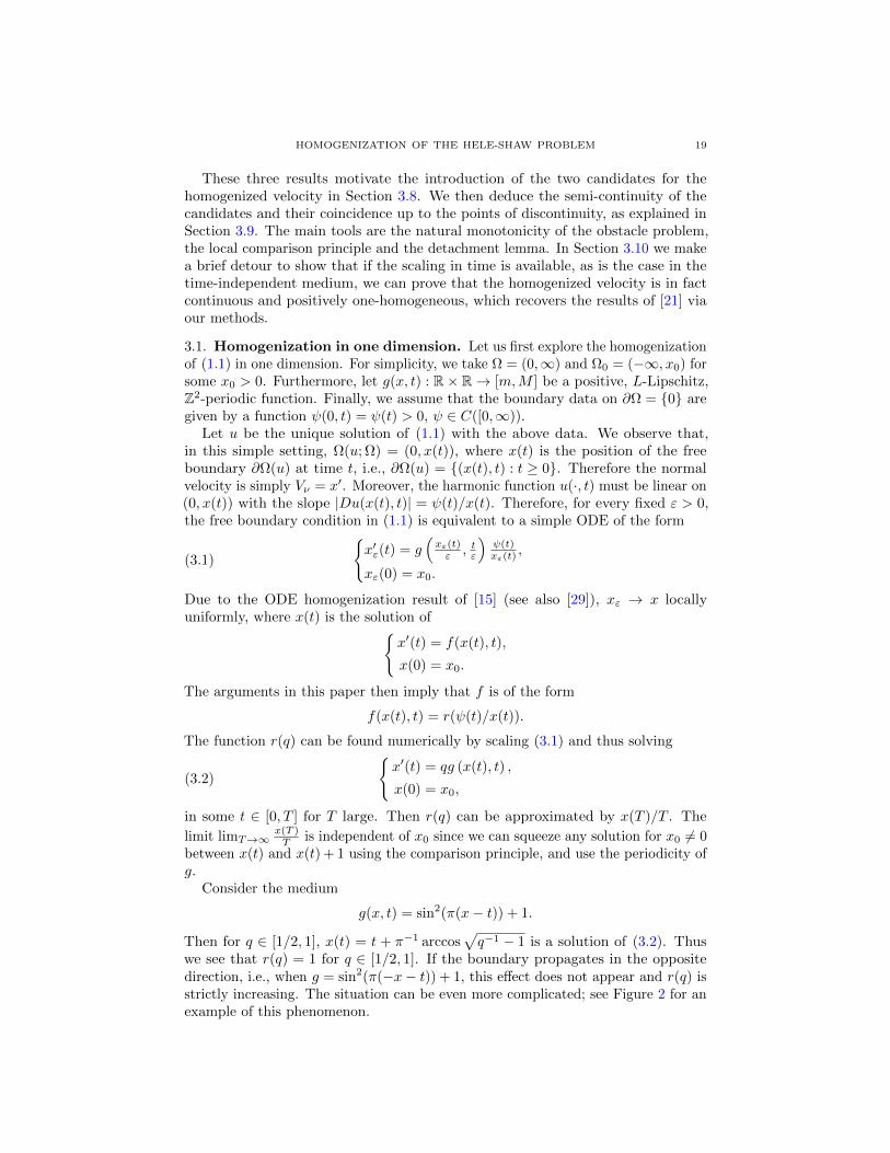
Consider the medium

g(x, t) = sin2(π(x− t)) + 1.

Then for q ∈ [1/2, 1], x(t) = t + π−1 arccos√q−1 − 1 is a solution of (3.2). Thus

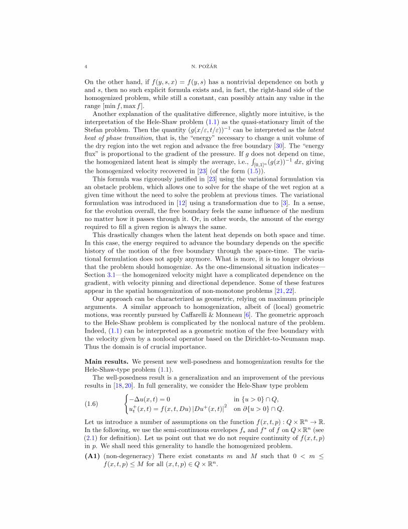
we see that r(q) = 1 for q ∈ [1/2, 1]. If the boundary propagates in the oppositedirection, i.e., when g = sin2(π(−x− t)) + 1, this effect does not appear and r(q) isstrictly increasing. The situation can be even more complicated; see Figure 2 for anexample of this phenomenon.

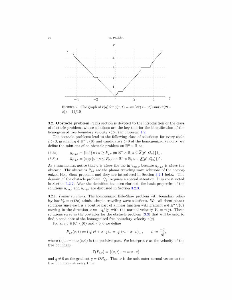
20 N. POZAR

−4 −2 2 4

1

2

3

4

r

−q

Figure 2. The graph of r(q) for g(x, t) = sin(2π(x−3t)) sin(2π(2t+x)) + 11/10

3.2. Obstacle problem. This section is devoted to the introduction of the classof obstacle problems whose solutions are the key tool for the identification of thehomogenized free boundary velocity r(Du) in Theorem 1.2.

The obstacle problems lead to the following class of solutions: for every scaleε > 0, gradient q ∈ Rn \ 0 and candidate r > 0 of the homogenized velocity, wedefine the solutions of an obstacle problem on Rn × R as

uε;q,r =(infu : u ≥ Pq,r on Rn × R, u ∈ S(gε, Qq)

)∗ ,(3.3a)

uε;q,r = (sup u : u ≤ Pq,r on Rn × R, u ∈ S(gε, Qq))∗ .(3.3b)

As a mnemonics, notice that u is above the bar in uε;q,r because uε;q,r is above theobstacle. The obstacles Pq,r are the planar traveling wave solutions of the homog-enized Hele-Shaw problem, and they are introduced in Section 3.2.1 below. Thedomain of the obstacle problem, Qq, requires a special attention. It is constructedin Section 3.2.2. After the definition has been clarified, the basic properties of thesolutions uε;q,r and uε;q,r are discussed in Section 3.2.3.

3.2.1. Planar solutions. The homogenized Hele-Shaw problem with boundary veloc-ity law Vν = r(Du) admits simple traveling wave solutions. We call them planarsolutions since each is a positive part of a linear function with gradient q ∈ Rn \ 0moving in the direction ν := −q/ |q| with the normal velocity Vν = r(q). Thesesolutions serve as the obstacles for the obstacle problem (3.3) that will be used tofind a candidate of the homogenized free boundary velocity r(q).

For any q ∈ Rn \ 0 and r > 0 we define

Pq,r(x, t) := (|q| rt+ x · q)+ = |q| (rt− x · ν)+ , ν :=−q|q|,

where (s)+ := max(s, 0) is the positive part. We interpret r as the velocity of thefree boundary

Γ(Pq,r) = (x, t) : rt = x · ν

and q 6= 0 as the gradient q = DPq,r. Thus ν is the unit outer normal vector to thefree boundary at every time.


The following observation is a trivial consequence of the nondegeneracy assump-tion (1.2).

Proposition 3.1. Pq,r ∈ S(gε) if

r ≤ m |q|

and Pq,r ∈ S(gε) if

r ≥M |q| .

Proof. Use (1.2).

In view of Proposition 3.1, we will often impose the following restriction on thevalues of r and q throughout the paper:

q 6= 0, m ≤ r

|q|≤M.(3.4)

Proposition 3.2. For given q 6= 0 and r > 0 we have

Pq,r(x− y, t− τ) ≤ Pq,r(x, t) for all x, t if and only if y · ν ≤ rτ,

and

Pq,r(x− y, t− τ) ≥ Pq,r(x, t) for all x, t if and only if y · ν ≥ rτ.

Proof. The statement is obvious from the identity

|q| (r(t− τ)− (x− y) · ν) = |q| (rt− x · ν) + |q| (y · ν − rτ),

and from the definition of Pq,r. To prove the only-if direction, consider x = 0 and tsufficiently large so that the first two terms above are positive.

3.2.2. Domain. In this section we construct a class of space-time cylinders Qq thatserve as the domains for the obstacle problem introduced in (3.3). The base ofthe cylinder is chosen to be a cone with a prescribed opening angle and an axis inthe direction that coincides with the normal of the free boundary of the obstacle.This particular choice of geometry will let us control how fast the solution of theobstacle problem detaches from the obstacle at the lateral boundary of the domainQq. It is achieved by a comparison with the class of planar subsolutions andsupersolutions R±ξ constructed below. In fact, this is the main motivation for thistechnical construction. With these barriers at our disposal, we can show that thefree boundaries of the solutions uε;q,r and uε;q,r must lie inside an intersection ofcertain cones; see Proposition 3.8. The ability to control the boundary behavior willbe necessary for the extension of the monotonicity property of the obstacle problembeyond the straightforward inclusion of domains. One of the main consequences ofthis extra monotonicity is the cone flatness property, Proposition 3.20.

Throughout the rest of this section, we fix q ∈ Rn \ 0 and r > 0 and let ν = −q|q| .

For simplicity, we shall denote

Γt = Γt(Pq,r).

Since the homogenization result is trivial when m = M , we may assume through-out the rest of the paper that 0 < m < M . We define angles θ, θ+ ∈ (0, π2 ), and

22 N. POZAR

Γt Iξ,t

V = −νθ

ν

η+

ξ

ϕ−

θ − ϕ−θ

η−

Ωq V −t

V +t

C−t

C+t

θ−

θ+

ξ−

ξ+

Figure 3. The cone Ωq and the support of the sub/supersolutionboundaries at a time t

θ− ∈ (θ, π2 ) as

θ = arccos

√m

M(3.5a)

θ+ =π

2− θ(3.5b)

θ− =π

2+ θ − ϕ−, where ϕ− := arccos

m

M.(3.5c)

Note that indeed θ− ∈ (θ, π2 ) since ϕ− ∈ (θ, π2 ) by cosϕ− = mM <

√mM = cos θ.

Let Conep,θ(x) be the open cone with axis in the direction of p ∈ Rn, openingangle 2θ and vertex x, that is,

Conep,θ(x) := y : (y − x) · p > |y − x| |p| cos θ.


Angles θ, θ+ and θ− then define cones Ωq, C+t and C−t for every t ≥ 0,

Ωq := Coneν,θ(V ),

C−t := Coneν,θ−(V −t ),

C+t := Cone−ν,θ+(V +

t ),

where V = −ν and the vertices V ±t are uniquely determined by the equality

Ωq ∩ Γt = C−t ∩ Γt = C+t ∩ Γt,(3.6)

see Figure 3. Finally, we define the space-time cylinder

Qq := Ωq × (0,∞).

Remark 3.3. Since the positions of the vertices V ±t of the cones C±t clearly dependlinearly on time, we can extend their definition to all t ∈ R as

V ±t = V ±0 + r±V tν t ∈ R,

where r±V are constants and we call them the velocities of V ±t . Note that V = V +−r−1 =

V −−r−1 = −ν due to (3.6) and the fact that V = −ν ∈ Γt(Pq,r) at t = − 1r. The velocities of

r±V can be found explicitly. Since the cones share a base, (3.6), we infer that (see Figure 3)

(r+V − r) tan θ+ = r tan θ = (r − r−V ) tan θ−.

Since θ+ = π2− θ, tan θ+ = 1

tan θholds and we have

r+V = r(1 + tan2 θ) =r

cos2 θ=M

mr > r.

We can similarly express the velocity r−V as

r−V =

(1− tan θ

tan θ−

)r = cM

mr ∈ (0, r).

The reason for this choice of domain Qq is the result in Lemma 3.7 below. But webegin with the following geometrical result. Let us introduce the set of all directionsof rays in ∂Ωq:

Ξ = ξ ∈ Rn : |ξ| = 1, ξ · ν = cos θ.(3.7)

Proposition 3.4. For any given x ∈ ∂Ωq, x 6= V , there exists unique ξ ∈ Ξ suchthat x ∈ Lξ ⊂ ∂Ωq, where Lξ is the ray

Lξ := σξ + V : σ ≥ 0.(3.8)

Furthermore, there exist unique ξ− and ξ+ such that |ξ±| = 1,

L±ξ,t :=σξ± + V ±t : σ ≥ 0

⊂ ∂C±t

and

L±ξ,t ∩ Lξ = Iξ,t for all t ≥ 0

for some point Iξ,t. Let η±ξ be the unit normal to ∂C±t on L±ξ,t with η± · ν > 0.

There exist unique constants µ±, r± and T± depending only on (q, r,m,M), andindependent of ξ, such that

Γt(R±ξ ) ∩ ∂C±t = L±ξ,t for all t ≥ 0,(3.9)

R±ξ = Pq,r on Lξ × [0,∞)(3.10)

24 N. POZAR

where

R±ξ (x, t) := P−µ±η±ξ ,r±(x, t− T±).(3.11)

Proof. The existence of ξ, ξ+, ξ− is straightforward.µ± and r± can be expressed using the following geometric considerations.By definition,

cos θ = ξ · ν.

We introduce ϕ± ∈ (0, π/2) via cosϕ± = ξ · η± and note that

θ+ =π

2+ ϕ+ − θ, θ− =

π

2+ θ − ϕ−.(3.12)

Observe that the point Iξ,t ∈ Lξ ∩ Γt moves in the direction ξ along Lξ with thevelocity rI given as

rI =r

cos θ.

Since R±ξ propagates in the direction η±, |η±| = 1, and

Iξ,t = L±ξ,t ∩ Lξ = Γt(R±ξ ) ∩ ∂C±t ∩ Lξ

by condition (3.9), we must have Iξ,t ∈ Γt(R±ξ ) for all t ≥ 0 and therefore

r± = rI(ξ · η±) = rI cosϕ± = rcosϕ±

cos θ.(3.13)

The slope µL of Pq,r on Lξ is

µL = |q| cos θ.

In (3.10) we require that this is also the slope of R±ξ on Lξ, i.e.,

µ± =µL

cosϕ±=|q| cos θ

cosϕ±.(3.14)

Finally, the constants T± are then fixed by requiring V ±T± = 0, and therefore, byRemark 3.3,

T± =1

r±V− 1

r.

It is straightforward to check that R±ξ defined with such unique choice of µ±, r±

and T± satisfy (3.9) and (3.10).

We complete the family of R±ξ defined in (3.11) by introducing two special planarfunctions:

R+0 (x, t) = Pq,max(M |q|,r)(x, t),

R−0 (x, t) = Pq,min(m|q|,r)(x, t).(3.15)

Corollary 3.5. We have

R−ξ ≤ Pq,r ≤ R+ξ on Qq for all ξ ∈ Ξ ∪ 0,

with equality

R±ξ = Pq,r on Lξ × [0,∞) ⊂ ∂Qq for ξ ∈ Ξ,

R±0 = Pq,r at t = 0,

where Lξ was introduced in (3.8).


Moreover,

supξ∈Ξ

R−ξ ≥ Pq,r ≥ infξ∈Ξ

R+ξ on Ωcq × [0,∞).(3.16)

Finally, ⋂ξ∈Ξ

Ωt(R+ξ ) = C+

t ,⋂ξ∈Ξ

Ωct(R−ξ ) = C−t for all t ≥ 0.(3.17)

Proof. Since the statement is obvious for ξ = 0 by the definition of R±0 in (3.15), wefix ξ ∈ Ξ. Let η be the unit normal vector to ∂Ωq on Lξ ⊂ ∂Ωq. Clearly η · ξ = 0.Define the half-space H := x : (x− V ) · η > 0 and observe that Ωq ⊂ H and∂Ωq ∩ ∂H = Lξ.

Let us first show that Pq,r = R±ξ on ∂H. We note that if x ∈ ∂H we can express

x− V = σξ + y, where σ ∈ R and y · ξ = y · η = 0. Since ν, η+, η− ⊂ span ξ, η,and Pq,r = R±ξ on Lξ by Proposition 3.4, linearity implies

Pq,r(x, t) = Pq,r(V + σξ + y, t) = Pq,r(V + σξ, t)

= R±ξ (V + σξ, t) = R±ξ (x, t) (x, t) ∈ ∂H × R.

Additionally, by linearity, since V ±t ∈ H for all t ≥ 0, and

V +t ∈ Ωt(R

+ξ ) \ Ωt(Pq,r), V −t ∈ Ωt(Pq,r) \ Ωt(R

−ξ ),

we must have

R−ξ ≤ Pq,r ≤ R+ξ on H × [0,∞) ⊃ Qq

and

R−ξ ≥ Pq,r ≥ R+ξ on Hc × [0,∞).

Since for every (x, t) ∈ Ωcq × [0,∞) there exists ξ ∈ Ξ such that x ∈ Hc, (3.16) is

also proved.To show one inclusion (⊃) of (3.17), we recall that by (3.9) and the choice

η± · ν > 0, we clearly have

C+t ⊂ Ωt(R

+ξ ), C−t ⊂ Ωct(R

−ξ ), t ≥ 0.

To show the other inclusion (⊂) of (3.17), we only need to show that for anyx ∈ Rn there exists ξ ∈ Ξ that generates ξ±, η± as in Proposition 3.4 and x can beexpressed as

x = α±ξ± + β±η± + V ±t ,(3.18)

and therefore clearly for such ξ we have

x /∈ C+t ⇔ β+ ≥ 0 ⇔ R+

ξ (x, t) = 0 ⇔ x /∈ Ωt(R+ξ ),

x /∈ C−t ⇔ β− < 0 ⇔ R−ξ (x, t) > 0 ⇔ x /∈ Ωct(R−ξ ).

To find such ξ for a given x ∈ Rn, first observe that there exists y ∈ ∂Ωq suchthat x = y + aν for some a ∈ Rn. Since y ∈ ∂Ωq, there exists ξ ∈ Ξ such thaty ∈ Lξ and therefore x = σξ + aν + V . Finally, we can write x as (3.18) sinceξ, ν, V ±t − V

⊂ span ξ±, η±. This concludes the proof.

The following geometrical observation, which shows a connection between thecones C±t and the planar functions R±ξ , will be useful later in deriving monotonicityproperties of the solutions of the obstacle problems.

26 N. POZAR

Proposition 3.6. For fixed a > 0, the following are equivalent (all with superscripteither + or −):

(a) ±aR±ξ (a−1x, a−1t) ≤ ±R±ξ (x− y, t− τ) for all ξ ∈ Ξ, (x, t) ∈ Rn × R;

(b) aC±a−1t ⊂ C±t−τ + y for some t ∈ R;

(c) y ∈ Cone±ν,θ±(r±V τν + (a− 1)V ±0 ) where r±V were introduced in Remark 3.3.

Proof. Clearly aR±ξ (a−1x, a−1t) is just a translation of R±ξ (x, t) by scaling invariance,

therefore we can compare the planar solutions in (a) by comparing their supports.In fact, we have

aV ±a−1t ∈ Γt(aR±ξ (a−1·, a−1·))

by construction and

Ωt(R±ξ (· − y, · − τ)) = Ωt−τ (R±ξ ) + y,

for all ξ ∈ Ξ. Therefore by Corollary 3.5 it is straightforward that (a) is equivalentto

aV ±a−1t ∈ C±t−τ + y for some t ∈ R.

This is clearly equivalent to (b) since aV ±a−1t is the vertex of aC±a−1t. And it is alsoequivalent to (c) if we take t = 0 and compute

aV ±0 ∈ C±−τ + y = Cone∓ν,θ±(V ±−τ + y).(3.19)

Since V ±−τ = V ±0 − r±V τν by Remark 3.3, we can rewrite (3.19) as (c).

The main motivation for such an involved choice of the domain for the obstacleproblem is the following observation on the properties of functions R±ξ .

Lemma 3.7. Suppose that q and r satisfy the condition (3.4). Then the choice ofthe angles θ, θ± in (3.5), depending only on m

M , guarantees that

R+ξ ∈ S(M) ⊂ S(gε) and R−ξ ∈ S(m) ⊂ S(gε) for all ξ ∈ Ξ ∪ 0,

where R±ξ were introduced in (3.11) and (3.15).

Proof. The statement is obvious for R±0 , by definition. For any ξ ∈ Ξ, by Propo-sition 3.1, we only need to verify r+ ≥Mµ+ and r− ≤ mµ−. Recall that q and rsatisfy (3.4).

We first observe that cosϕ+ = 1 by (3.12) and (3.5b). Then, in order, (3.13),(3.14), (3.5a), and finally (3.4) lead to

r+

µ+=

r

|q|cos2 ϕ+

cos2 θ=

r

|q|M

m≥M,

which verifies that R+ξ ∈ S(M).

Similarly, (3.13), (3.14), (3.5a), (3.5c) and (3.4) yield

r−

µ−=

r

|q|cos2 ϕ−

cos2 θ=

r

|q|m

M≤ m,

which verifies that R−ξ ∈ S(m).


3.2.3. Properties of the obstacle solutions. The basic properties of the solutionsuε;q,r and uε;q,r of the obstacle problem introduced in (3.3) are gathered in thefollowing proposition.

Proposition 3.8. For any q ∈ Rn \ 0, r > 0 satisfying (3.4) and any ε > 0, thefollowing statements apply.

(a) uε;q,r ∈ S(gε, Qq) and uε;q,r ∈ S(gε, Qq \ (Γ(uε;q,r) ∩ Γq,r));

(b) uε;q,r ∈ S(gε, Qq) and uε;q,r ∈ S(gε, Qq \ (Γ(uε;q,r) ∩ Γq,r));(c) (uε;q,r)

∗ ≥ uε;q,r ≥ Pq,r and (uε;q,r)∗ ≤ uε;q,r ≤ Pq,r in Rn×R, with equalityon (Rn × R) \Qq;

(d) Ωt(uε;q,r) ⊂ C+t ∪ Ωt(Pq,r) and Ωct(uε;q,r) ⊂ C−t ∪ Ωct(Pq,r);

(e) uε;q,r ∈ S(M,Rn × R) and uε;q,r ∈ S(m,Rn × R);

(f) uε;q,r ≤ infξ∈Ξ∪0R+ξ and uε;q,r ≥ supξ∈Ξ∪0R

−ξ on Qq.

Proof. (a) and (b) are standard; see [20, Lemma 4].To prove (c), we recall the definition of R±ξ in (3.11) and (3.15). Lemma 3.7 and

Corollary 3.5 yield that max(Pq,r, R+ξ ) ∈ S(gε, Qq) and min(Pq,r, R

−ξ ) ∈ S(gε, Qq)

and thus, by definition,

uε;q,r ≤ max(Pq,r, R+ξ ), uε;q,r ≥ min(Pq,r, R

−ξ ) for all ξ ∈ Ξ ∪ 0,(3.20)

which proves (f). Therefore Corollary 3.5 implies that

(uε;q,r)∗ = uε;q,r = (uε;q,r)∗ = uε;q,r = Pq,r on (Rn × R) \Qq,

and (c) is proved.The result of (d) follows from (3.20), using the support property of R±ξ in (3.17).

Since q and r satisfy (3.4), (e) follows from (a)–(b) and Proposition 3.1.

Remark 3.9. Fix T > 0 and a pair q, r that satisfies (3.4). We shall show that uε;q,rcoincides with the function defined on QT = Qq ∩ t < T,

v =(

infu ∈ S(gε, QT ) : u ≥ Pq,r on QT

)∗,QT

,

which is the solution of the obstacle problem considered in [20]. An analogous result holdsfor uε;q,r.

Indeed, v ≤ uε;q,r trivially, but also, since v ≤ R+ξ on Q

T, we can define for any s < T

the function

w(x, t) =

v(x, t) t ≤ s,R+

0 (x, t) t > s.

Clearly w ∈ S(gε, Qq) and hence, by definition, uε;q,r ≤ w = v for t ≤ s for any s < T .

3.3. Monotonicity of the obstacle problem. The solutions uε;q,r and uε;q,r ofthe obstacle problem introduced in (3.3) admit a natural monotonicity property withrespect to the hyperbolic scaling and a change of scale ε. Moreover, the periodicityof the medium also yields the monotonicity with respect to translations by multipliesof ε, both in space and time. Since we have a control on how fast the free boundariesof uε;q,r and uε;q,r detach from the obstacle at the parabolic boundary of the domainQq, we can extend the allowed range of translations. This is the main result of thissection. The second result is the monotonicity of uε;q,r and uε;q,r in time.

28 N. POZAR

Proposition 3.10 (Monotonicity). Let q and r satisfy (3.4), and let a > 0. Then

uε;q,r(x, t) ≤ a−1uaε;q,r(a(x− y), a(t− τ))

for all (x, t) ∈ Rn × R and for all (y, τ) ∈ εZn+1 such that

y · ν ≥ max(rτ,M |q| τ), and y ∈ Coneν,θ+(r+V τν + (a− 1)V +

0 ),(3.21)

where r±V , V ±0 and θ± were defined in Section 3.2.2.Similarly,

uε;q,r(x, t) ≥ a−1uaε;q,r(a(x− y), a(t− τ))

for all (x, t) ∈ Rn × R and for all (y, τ) ∈ εZn+1 such that

y · ν ≤ min(rτ,m |q| τ), and y ∈ Cone−ν,θ−(r−V τν + (a− 1)V −0 ).(3.22)

Proof. We shall show the ordering for uε;q,r, the proof for uε;q,r is analogous.Fix a > 0 and (y, τ) that satisfies the hypothesis (3.21) and define the cylinder

Σ = Qq ∩ (a−1Qq + (y, τ)).

Let us, for simplicity, denote

va(x, t) := a−1uaε;q,r(a(x− y), a(t− τ)).

Due to the εZn+1-periodicity of gε, we observe that va ∈ S(gε, a−1Qq + (y, τ)). Weimmediately have

Pq,r(x, t) ≥ Pq,r(x− y, t− τ) = a−1Pq,r(a(x− y), a(t− τ)) ≥ va(x, t)(3.23)

by (3.22), the scale invariance and Proposition 3.2.Our goal is to show that

uε;q,r ≥ va on Σc and Ω(va) ∩ Σc ⊂ Ω(uε;q,r)(3.24)

since then we can apply Lemma 2.17 with Q1 = Σ, Q2 = Qq, u1 = va and u2 = uε;q,rto conclude that u ∈ S(gε, Qq), where u is defined in Lemma 2.17. Because clearlyu ≤ Pq,r by (3.23), we have by definition of uε;q,r that uε;q,r ≥ u ≥ va on Σ andtherefore uε;q,r ≥ va on Rn × R.

Let us prove (3.24). We can write Σc = A1 ∪ A2 ∪ A3 where A1 := (Qq)c,

A2 := Qq ∩ ((a−1Ωq + y)c × [τ,∞)) and A3 := Qq ∩ t < τ. We therefore proveuε;q,r(x, t) ≥ va(x, t) for all (x, t) ∈ Σc by considering the following three cases:

• (x, t) ∈ A1: This case is very simple since Proposition 3.8(c) and (3.23),yield

uε;q,r(x, t) = Pq,r(x, t) ≥ va(x, t).

• (x, t) ∈ A2: Observe that (3.22) implies Proposition 3.6(c) and thereforeProposition 3.6(a) holds. We use Proposition 3.8(f), Proposition 3.6(a) and(3.16), all properly rescaled, and estimate

uε;q,r(x, t) ≥ supξ∈Ξ

R−ξ (x, t) ≥ supξ∈Ξ

a−1R−ξ (a(x− y), a(t− τ))

≥ a−1Pq,r(a(x− y), a(t− τ)) ≥ va(x, t).


• (x, t) ∈ A3: Since 0 ≤ t ≤ τ , Proposition 3.8(f) and (3.22) yield

uε;q,r(x, t) ≥ R−0 (x, t) = |q| (m |q| t− x · ν)+

≥ |q| (r(t− τ)− (x− y) · ν)+ = a−1Pq,r(a(x− y), a(t− τ))

≥ va(x, t).

Therefore we have shown the first part of (3.24), and the second part can beinferred from the above estimates as well. Consequently, the argument usingLemma 2.17 described above applies and we can conclude that uε;q,r ≥ va onRn × R.

The second important result of this section is the almost obvious fact that thesolutions of the obstacle problems are increasing in time. However, in contrast to[20], Proposition 3.10 only implies the monotonicity in time for multiplies of ε due tothe time-dependence of g. Here we present an argument using a nonlinear scaling ofthe solutions, which also provides a lower bound on the speed of the free boundary.

Lemma 3.11 (Monotonicity in time). Let r and q satisfy (3.4) and let ε > 0. Then

uε;q,r(x− y, t1) ≤ uε;q,r(x, t2),

uε;q,r(x− y, t1) ≤ uε;q,r(x, t2)

for any t1 < t2 and x ∈ Rn, and y ∈ Rn such that |y| ≤ ρ for some positive constantρ depending only on m,L, ε, t1, t2.

Proof. Let us fix r, q and ε. We first prove the result for u := uε;q,r. Since wehave to compare solutions that are not necessarily translated by a multiply of ε, wecannot use the monotonicity of Proposition 3.10 directly. Instead, we will compareu with its nonuniform perturbation using Proposition B.1.

First, assume that 0 < t1 < t2 < t1 + γ where γ := mL . We shall define

v(x, t) = infy∈Bρ(0)

uε;q,r(x− y, θ(t)),(3.25)

where ρ will be a positive constant and θ(t) := θ(t; λ) = λ + f(t; λ) for some λdetermined below. Function f(t;λ) is the function constructed in Section B.2 forgiven parameters γ (defined above), a = 1, and λ > 0. Because Dρ ≡ 0 we setα = a = 1.

With these parameters, the expression for θ(t;λ) is simply

θ(t;λ) = t− γW(−λγe−

λγ e

tγ

),

where W is the Lambert W function. Therefore θ(t;λ) is well-defined on t ∈ [0, tλ]and λ ∈ [0, γ], where tλ := log γ

λ+ λγ −1 (we set t0 = +∞). Observe that tλ is strictly

decreasing in λ and positive for λ ∈ (0, γ] with tλ = 0 at λ = γ and tλ → +∞ asλ→ 0+. Therefore for every t > 0 there exists a unique λ =: λt such that tλ = t.From the properties of W , we observe that θ(t; 0) = t and θ(t;λt) = t+ γ for anyt > 0. By continuity and the assumption t2 ∈ (t1, t1 + γ), there exists λ ∈ (0, λt1)such that θ(t1; λ) = t2. Since λ < λt1 we must have tλ > t1.

Let us thus take θ(t) = θ(t; λ) and consider uε;q,r(x−y, θ(t)) for some y ∈ Rn and(x, t) ∈ t ≤ tλ. It was shown in the proof of Proposition 3.10 that uε;q,r(x, t) ≤uε;q,r(x− y, t− τ) on (Qq ∩ (Qq + (y, τ))c for all (y, τ) satisfying (3.21). Let us set

τ = −λ. There exists ρ > 0 such that (y, τ) satisfies (3.21) for all y ∈ Bρ(0). Since

30 N. POZAR

t+λ ≤ θ(t) for all t ∈ [0, tλ], the same argument yields uε;q,r(x, t) ≤ uε;q,r(x−y, θ(t))on (Qq ∩ (Qq + (y, τ))c ∩ t ≤ tλ for (y, τ) ∈ Bρ(0)×

−λ

. Hence the argumentusing Lemma 2.17 as in the proof of Proposition 3.10 (with Remark 3.9 for extensionof v for t > tλ) yields that uε;q,r(x, t) ≤ uε;q,r(x− y, θ(t)) for (x, t) ∈ t < tλ. In

particular u(x, t1) ≤ u(x − y, θ(t1)) = u(x − y, t2) for all y ∈ Bρ(0), and that iswhat we wanted to prove.

The proof for general 0 < t1 < t2 can be done iteratively by splitting [t1, t2] intosubintervals of length smaller than γ.

We skip the proof for uε;q,r, which follows the same idea, but is simpler. Inparticular, it is unnecessary to restrict t2 < t1 + γ since f constructed in Section B.1can handle arbitrary tranlations.

For completeness, and as a consequence of the monotonicity in time in theprevious lemma, we also show that the solutions are harmonic in their positive sets.

Proposition 3.12. Let r and q satisfy (3.4) and let ε > 0. The functions uε;q,r(·, t)and (uε;q,r)∗ (·, t) are harmonic in Ωt(uε;q,r)∩Ωq and Ωt((uε;q,r)∗)∩Ωq, respectively,for every t.

Proof. Since the claim is trivially true for t ≤ 0, we fix τ > 0. We first show thatuε;q,r(·, τ) is harmonic in the open set E := Ωτ (uε;q,r) ∩ Ωq. For any w ∈ LSC(E),superharmonic in E, such that w ≥ uε;q,r(·, τ) on ∂E, we define a new function onQq ∩ t ≤ τ

v(x, t) =

min

(uε;q,r(x, t), w(x)

)x ∈ E,

uε;q,r(x, t) otherwise.

By definition of w, we observe that v ∈ LSC(Qq ∩ t ≤ τ) and v ∈ S(gε, Qq ∩t ≤ τ). Therefore uε;q,r(x, τ) ≤ v(x, τ) ≤ w(x) in E by definition of uε;q,r andRemark 3.9. We recall that uε;q,r(·, τ) is superharmonic in E, and therefore it isthe smallest superharmonic function, i.e., it must be harmonic.

Now we show that (uε;q,r)∗(·, τ) is harmonic in the open set E = Ωτ ((uε;q,r)∗)∩Ωq.

First we recall that (uε;q,r)∗(·, τ) is superharmonic since uε;q,r ∈ S(m,Rn × R) by

Proposition 3.8. Let w ∈ LSC(E) be a superharmonic function in E, such thatw ≥ (uε;q,r)∗(·, τ) on ∂E. By the monotonicity in time, Lemma 3.11, and inparticular the positive speed of expansion, we observe that uε;q,r(x, t) = 0 forx ∈ Γτ ((uε;q,r)∗) and t < τ . Since uε;q,r(·, t) is subharmonic in Ωq for all t, wemust have uε;q,r(x, t) ≤ w(x) for t < τ . Therefore, (uε;q,r)∗(x, τ) ≤ w(x). Again,(uε;q,r)∗(·, τ) is the smallest superharmonic function and thus harmonic.

3.4. Flatness. In this section we introduce flatness, the quantity that will be ameasure of how good our guess of the homogenized velocity r(q) is. More specifically,it measures how far, for given ε, q and r, the free boundaries of the obstacle problemsolutions uε;q,r and uε;q,r, introduced in (3.3), detach from the free boundary of theobstacle Pq,r up to the given time.

For η ∈ R, denote

P ηq,r(x, t) := Pq,r(x− ην, t).

Note that P ηq,r represents a translation of Pq,r in the direction ν by distance η.


Definition 3.13. For q 6= 0, r > 0 and ε > 0, we define the upper flatness Φε;q,r(τ),i.e., the flatness of uε;q,r up to time τ ∈ R as

Φε;q,r(τ) = infη : uε;q,r ≤ P ηq,r in t ≤ τ

.

Similarly, the lower flatness Φε;q,r(τ) is defined as the flatness of uε;q,r up to timeτ ∈ R,

Φε;q,r(τ) = infη : uε;q,r ≥ P−ηq,r in t ≤ τ

.

We say that uε;q,r (resp. uε;q,r) is η-flat up to time τ if Φε;q,r(τ) ≤ η (resp.

Φε;q,r(τ) ≤ η).

The flatness is Lipschitz and monotone:

Proposition 3.14. Let q ∈ Rn \ 0, r > 0 and ε > 0. Then for any t ∈ R, h > 0,

Φε;q,r(t) ≤ Φε;q,r(t+ h) ≤ Φε;q,r(t) + h(M |q| − r)+,

Φε;q,r(t) ≤ Φε;q,r(t+ h) ≤ Φε;q,r(t) + h(r −m |q|)+.

In particular, Φε;q,r and Φε;q,r are nondecreasing and Lipschitz continuous.

Proof. Φε;q,r and Φε;q,r are clearly nondecreasing from their definition.To show the upper bound for Φε;q,r(τ + h) for any τ ∈ R, h > 0, we may

assume that r < M |q|, otherwise uε;q,r = Pq,r and so Φε;q,r(τ + h) = Φε;q,r(τ) =

0. We only need to compare uε;q,r with an appropriate translation of R+0 =

Pq,M |q|, using the fact that uε;q,r(·, τ) ≤ P ηq,r(·, τ) and the identity Pq,M |q|(·, h) =

P(M |q|−r)hq,r (·, h). Similarly, the upper bound for Φε;q,r(τ+h) follows from comparison

with a translation of R−0 = Pq,m|q|.

Finally, we can always find a point on the free boundary of uε;q,r or uε;q,r whosespatial distance from the free boundary of the obstacle is exactly equal to the flatnessat the given time.

Lemma 3.15. Let q ∈ Rn \ 0, r > 0 and ε > 0. Let τ ∈ R. Then forany η ∈ (0,Φε;q,r(τ)] there exists (ζ, σ) ∈ Γ(uε;q,r) such that ζ · ν = rσ + η and

Φε;q,r(t) ≤ η for all t ≤ σ. Similarly, for any η ∈ (0,Φε;q,r(τ)] there exists

(ζ, σ) ∈ Γ(uε;q,r) such that ζ · ν = rσ − η and Φε;q,r(t) ≤ η for all t ≤ σ.

Proof. We will show the proof for uε;q,r, the proof for uε;q,r is similar.

Let us define T = supt ≤ τ : Φε;q,r(t) ≤ η

. Clearly T ∈ (0, τ ]. Moreover,

by continuity, Φε;q,r(T ) = η. We claim that we can find (ζ, σ) ∈ Ωc(P ηq,r) ∩Ω(uε;q,r) ∩ t ≤ T. If such point does not exist, we must have dist(Ωc(P ηq,r) ∩0 ≤ t ≤ T,Ω(uε;q,r)) > 0 and therefore there exists δ ∈ (0, η) such that Ωc(P η−δq,r )∩Ω(uε;q,r) ∩ t ≤ T = ∅. Since P η−δq,r is harmonic in its positive set, it follows that

uε;q,r ≤ P η−δq,r in t ≤ T. But that is a contradiction with Φε;q,r(T ) = η >η − δ. Therefore (ζ, σ) exists and we observe that (ζ, σ) ∈ Γ(uε;q,r) ∩ Γ(P ηq,r) ∩0 < t ≤ T.

32 N. POZAR

3.5. Local comparison principle. An important tool in the analysis of the behav-ior in the homogenization limit is the local comparison principle. In contrast to thestandard comparison principle, which requires ordering on the parabolic boundaryto guarantee ordering in the whole cylinder, the local comparison relies on the extrainformation about flatness of solutions in the sense of Definition 3.13, and thereforeallows for solutions to cross on the lateral boundary but still guarantees the orderingof free boundaries for a short time in a small region far from the boundary. This isa generalization of a result that appeared in [20,21] (with β = 1).

Theorem 3.16 (Local comparison principle). Let β ∈ ( 45 , 1), r1 > r2 > 0 and

q1, q2 ∈ Rn such that a3q1 = q2 for some a > 1.Then there exists ε0 = ε0(r1, r2, |q1| , |q2| ,m,M, n, β) such that

max(Φε;q1,r1(1),Φε;q2,r2(1)

)> εβ for ε < ε0.

In other words, uε;q1,r1 and uε;q2,r2 cannot be both εβ-flat up to time t = 1 for anyε < ε0.

Before proceeding with the proof of Theorem 3.16, we first present a simple resulton the nondegeneracy of uε;q,r. This is an improvement of Corollary A.5 when we

also know that uε;q,r is εβ-flat.

Lemma 3.17. For given q ∈ Rn \ 0, r > 0, there exists a positive constantc = c(r, |q| ,M, n) such that if Φε;q,r(T ) ≤ η, for some ε, η, T > 0, then

uε;q,r(x, t) ≥ cρ2

η

for every 0 < ρ ≤ η and (x, t) such that Bρ(x) ⊂ Ωt(uε;q,r) ∩ Ωq, t ≤ T .

Proof. Let cH = cH(n) be the constant from Harnack inequality such that if ψ ≥ 0,harmonic in B1(0) then infB1/2(0) ψ ≥ cH supB1/2(0) ψ.

Let us denote u = uε;q,r. Fix (ξ, τ) such that Bρ(ξ) ⊂ Ωτ (u)∩Ωq. Then we havetwo possible scenarios:

(a) ξ · ν ≤ rτ + ρ4 : We estimate

u(ξ − ρ

2ν, τ) ≥ Pq,r(ξ −

ρ

2ν, τ) ≥ |q| ρ

4≥ |q|

4

ρ2

η.

(b) ξ · ν > rτ + ρ4 : In this case necessarily r < M |q|, otherwise u = Pq,r, a

contradiction. We have u ∈ S(M,Rn × R) by Proposition 3.8 and u isnondecreasing in time by Lemma 3.11. Due to the flatness assumptionΦε;q,r(τ) ≤ η, u(·, t) = 0 on Bρ/4(ξ) for t ≤ τ − η

r . Consequently, Corol-lary A.5 implies

supBρ/4(ξ)

u(·, τ) ≥ ρ2

32nM ηr

=r

32nM

ρ2

η.

Since u(·, τ) is harmonic in Ωτ (u) ∩ Ωq ⊃ Bρ(ξ), the Harnack inequality, properlyrescaled, yields

u(ξ, τ) ≥ cH min

(|q|4,

r

32nM

)ρ2

η.

An important tool in the proof of the local comparison principle is the nonuniformperturbation in space, see Section B. We will construct a particular radius ρ(x) inthe following lemma.


Lemma 3.18. There exists R > 0 and a smooth, radially symmetric functionρ : B2R(0) \BR(0)→ [1, 6] such that ρ∆ρ ≥ (n− 1) |Dρ|2 in B2R(0) \BR(0), ρ = 1on ∂B2R(0) and ρ > 5 on BR+1(0) \BR(0).

Proof. Let ϕ be the radially symmetric smooth positive solution of∆ϕ2−n = 0, in B2 \B1

ϕ = 1 on ∂B2,

ϕ = 6 on ∂B1.

It was observed in [5, p. 148] that ϕ satisfies ϕ∆ϕ ≥ (n − 1) |Dϕ|2. Moreover,note that also the rescaled function aϕ(bx) satisfies the same inequality for any a, bpositive. By continuity, there exists δ > 0 such that ϕ > 5 on B1+δ \ B1. DefineR = 1/δ and ρ(x) = ϕ(δx) on B2R \ BR. It is straightforward to verify that ρsatisfies the properties asserted in the statement and the proof is finished.

The following technical lemma shows that the closure of a time-slice of Ω(uε;q,r)is the time-slice of the closure, a fact that will be used throughout the proof of thelocal comparison principle and that allows us to work with simple time-slices of asubsolution with nondecreasing support.

Lemma 3.19. Let u ∈ S(M,Q) be a bounded subsolution on Q for some M > 0and Q = E × (t1, t2), E ⊂ Rn open, and assume that Ωt(u

∗) ⊂ Ωs(u∗) for all t, s

such that t1 < t ≤ s < t2. Then for any (x, t) ∈ Q we have

x ∈ Ωt(u∗;Q) if and only if (x, t) ∈ Ω(u;Q),

or, equivalently,

Ωt(u∗;Q) = Ωt(u;Q).

Proof. Since Ω(u) = Ω(u∗), we can WLOG assume that u = u∗. Let (ξ, τ) ∈ Q. It

is clear that if ξ ∈ Ωτ (u) then (ξ, τ) ∈ Ω(u). Now suppose that (ξ, τ) ∈ Ω(u) ∩Q.

By Definition 2.3(i) and the monotonicity assumption, (ξ, τ) ∈ Ω(u) ∩ t < τ ⊂Ωτ (u)× t ≤ τ.

Proof of Theorem 3.16. The proof proceeds in a number of technical steps.Suppose that such ε0 does not exist and both uε;q1,r1 and uε;q2,r2 are εβ-flat up to

time t = 1 along some subsequence of ε that converges to 0. We will show that thisleads to a contradiction with the comparison principle for the Hele-Shaw problemfor ε sufficiently small.

(1) Setup. Let α := 45 , and observe that, since β ∈ (4/5, 1),

2− 2β ≤ 4− 4β < α < β.(3.26)

First, for fixed ε > 0, we introduce notation that will be used throughout theproof. Symbol c with a subscript will denote quantities independent of ε.

We shall use multiple perturbations of the subsolution uε,q1,r1 . Throughout the

proof, ν = −q1|q1| = −q2

|q2| . Let us denote Λ := 6 and define the constant

γ =1

Λmin

(m

L(a1/2 − 1),

1

2

)(3.27)

34 N. POZAR

and a translation

ξ0 ∈ arg minξ∈εZnξ·ν≤−ε

|ξ| .

Clearly |ξ0| ≤ nε. For λ ∈ [0,Λ], we define the perturbations

uλ(x, t) := supy∈Bλγε(x)

auε,q1,r1(y − ξ0, t),

where B0(x) := x for simplicity. The choice of γ and ξ0, and Proposition B.1 imply

that uλ ∈ S(gε, Q), where Q :=

(x, t) : B(n+1)ε(x)× t ⊂ Qq

. Furthermore,

since γ ≤ 12Λ we note that uλ ≤ Paq1,r1 for all λ ∈ [0,Λ].

Next, we introduce the time

T :=3εβ

r1 − r2= cT ε

β > 0.

If ε is small enough so that T ≤ 1 then uλ and v will be (εβ + nε)-flat and εβ-flat,respectively, up to time t = T , and if also εβ ≥ nε ≥ |ξ0 · ν| then the free boundaryof uλ must completely overtake the free boundary of v by time T .

Finally, we choose the constants σ1, σ2 as

σ1 :=3a |q1|+ 1

|q2| − a |q1|εβ = cσ1

εβ ,

σ2 := Tr1 = cσ2εβ .

Let us also denote σ := σ1 + σ2 and remark that σ = cσεβ . The motivation behind

this particular choice of σ1 is the fact that

v(x, t)− uλ(x, t) ≥ Pq2,r2(x, t)− Paq1,r1(x, t) ≥ εβ(3.28)

for x · ν ≤ −σ1, t ∈ [0, T ], λ ≤ Λ. Similarly, σ2 is motivated by

Ωt(Paq1,r1) ∪ Ωt(Pεβ

q2,r2) ⊂ x : x · ν ≤ σ2(3.29)

for t ∈ [0, T ], i.e. the free boundaries of uε;q1,r1 and uε;q2,r2 will be contained inx : 0 ≤ x · ν ≤ σ2 for t ∈ [0, T ].

(2) Fast-shrinking domain. For a point x ∈ Rn, we define x⊥ to be the componentof x orthogonal to ν,

x⊥ = x− (x · ν)ν = (I − ν ⊗ ν)x.

By symbol Cyl(ρ; η1, η2) we shall denote the open space cylinder of radius ρ withaxis parallel to ν, between the hyperplanes x : x · ν = η1 and x : x · ν = η2,

Cyl(ρ; η1, η2) =x :∣∣x⊥∣∣ < ρ, η1 < x · ν < η2

.

Let us define a “fast-shrinking” domain Σ, whose each time-slice Σt is the cylinder

Σt :=

Cyl(ρΣ(t);−σ1, σ2) t ≥ 0,

∅ t < 0.

with radius

ρΣ(t) =tan θ

2− ε−αt,

where θ is the opening of the cone Ωq defining Qq, introduced in (3.5a). In particular,the radius ρΣ(t) of the cylinder Σt shrinks with velocity ε−α. Furthermore, if ε is


small enough, we have Σ + (B(n+1)ε × 0) ⊂ Qq, which also implies uλ ∈ S(gε,Σ)for λ ∈ [0,Λ]. Additionally, Σt 6= ∅ for all t ∈ [0, T ] since, as α < β by (3.26),

ρΣ(T ) =tan θ

2− ε−αT =

tan θ

2− cT εβ−α > 0 for ε > 0 small.

Finally, we need to fix a small time step τ ,

τ :=γ2ε2

4naσ |q1|M= cτε

2−β .(3.30)

Let us explain how such choice of τ guarantees that, for λ ∈ [0,Λ], the support ofuλ cannot expand by more than γε from time t− τ to time t for any t ∈ [τ, T ] inthe sense

Ωs(uλ) ⊂ Ωt−τ (uλ) +Bγε s ∈ [t− τ, t].(3.31)

This follows from a straightforward application of Corollary A.6, on the paraboliccylinder

E =

(x, t) : −σ1 < x · ν, t > t− τ,

taking advantage of the bound

uλ(x, t) ≤ Paq1,r1(x, t) ≤ a |q1|σ =: cKεβ ,(3.32)

valid for x · ν ≥ −σ1 and t ∈ [0, T ] due to (3.29).

(3) Boundary crossing point. With these definitions at hand, we proceed withthe proof. As we observed above, since nε ≤ εβ if ε is small enough, uλ is (εβ + nε)-flat for any λ ∈ [0,Λ], and v is εβ-flat, the choice of ξ0 and T guarantees that thesupports of uλ and v are originally strictly ordered, but will cross each other beforethe time T in the domain Σ. So let t be the first time that the boundaries of u5

and v touch in Σ, i.e.,

t := sups : Ω(u5) ∩ Ωc(v) ∩ Σ ∩ t ≤ s = ∅

< T.

Observe that t ≥ τ since Ωt(u5) cannot advance more than γε in time τ by (3.31).

We claim that the set Ωt(u5) ∩ Ωc

t(v) ∩ Σt is nonempty. Indeed, if that were not

the case, dist(Ωt(u5),Ωc

t(v) ∩ Σt) > 0 because the first set is closed and the second

one is compact. Therefore, there exists δ > 0 such that the distance is positivefor t < t+ δ by Corollary A.6 and the monotonicity of Ωc

t(v) ∩ Σt, which yields acontradiction with the definition of t. Let us thus choose

x ∈ Ωt(u5) ∩ Ωc

t(v) ∩ Σt.

We will show that the existence of such point leads to a contradiction with thecomparison principle for the Hele-Shaw problem since u5 and v were strictly separatedon a much larger domain Σt−τ at time t = t− τ .

To make this idea rigorous, we introduce the cylinders

Si = Cyl(ρi;−σ1, σ2) for i = 1, 2,

(see Figure 4) with radii

ρ1 := ρΣ(t− τ)− 2γε, ρ2 := ρ1 −(cKcN

ε2β−2 + 2

)cσε

β ,

36 N. POZAR

S2 S1

Σt−τ

Σt

xϕ

x

ν

σ

x · ν > σ2

x · ν < −σ1

Aϕ

ρ>

5γε

ε−ατ

Figure 4. Arrangement of cylinders

where constant cN is specified below in (3.35). We point out that if ε is smallenough, we have

ρ2 > ρΣ(t) + 2Rσ,(3.33)

where R is the constant from Lemma 3.18, since

ρΣ(t− τ)− ρΣ(t) = τε−α = cτε2−α−β ρΣ(t− τ)− ρ2 + 2Rσ if ε 1

due to (3.26). In particular, we have

Σt−τ ⊃ S1 ⊃ S2 ⊃ Σt,

see Figure 4.Now we consider function u2. First, clearly Ωt(u

5) = Ωt(u2) + B3γε(0). The

definition of t yields Ωt(u5) ∩ Ωct(v) ∩ Σt = ∅ for t < t, and thus, in particular,(

Ωt−τ (u2) +B3γε(0))∩ Ωc

t−τ (v) ∩ Σt−τ = ∅.

As Ωct(v) cannot expand (due to the monotonicity, Lemma 3.11), and the positive setof u2 cannot expand by more than γε in time τ , in the sense of (3.31), we concludethat

(Ωt(u2) +B2γε(0)) ∩ Ωct(v) ∩ S1 = ∅ t ∈ [0, t].(3.34)

Let us define the closed sets

At :=(Ωt(u

2) +Bγε(0))∩ S1 t ∈ [0, t].

Due to the nondegeneracy of v (Lemma 3.17 applied with η = εβ and ρ = γε), weobserve that

v(x, t) ≥ c(r2, |q2| ,M, n)γ2ε2−β = cNε2−β x ∈ At, t ∈ [0, t],(3.35)

where c(r2, |q2| ,M, n) is the constant from Lemma 3.17. Consider the function

wt(x) = u2(x,t)−v(x,t)cNε2−β

defined on At. Function wt is subharmonic on At for all

t ∈ [0, t] since v(·, t) is superharmonic in intAt as At ⊂ Ωt(v) ∩ Ωq, and u2(·, t) isclearly subharmonic in intAt.

Our goal is to apply Lemma C.1 to function wt. Since ε is small, we haveεβ ≥ cNε2−β and thus wt ≤ −1 on ∂At ∩ x : x · ν = −σ1 by (3.28). Additionally,u2 = 0 on ∂At ∩ S1 by definition of At and therefore wt ≤ −1 on ∂At ∩ S1. Finally,by (3.32),

wt ≤ u2

cNε2−β ≤cKcN

ε2β−2 on At.


Therefore Lemma C.1 implies that wt < 0 on the set S1 ∩x :∣∣x⊥∣∣ ≤ ρ′1, where

ρ′1 is given by

ρ′1 = ρ1 − cT(cKcN

ε2β−2 + 2

)cσε

β ,

and ρ′ ≥ ρ2 by the choice of ρ1 and ρ2. We conclude that wt < 0 in S2 ∩At for allt ∈ [0, t], and therefore, with (3.34),

u2 ≺ v in S2 × [0, t].(3.36)

Let R and ρ(x) be from Lemma 3.18 and define

xϕ := x⊥ + (σ2 +Rσ)ν

and

ϕ(x) := γερ

(x− xϕσ

)on Aϕ := B2Rσ(xϕ) \BRσ(xϕ).

Let us set cρ = maxB2R(0)\BR(0) |Dρ| <∞. Clearly

maxAϕ

|Dϕ| = γε

σcρ =

cρcσγε1−β .

Hence for ε small enough we have

(1−maxAϕ

|Dϕ|)−2 ≤ a1/2.(3.37)

Moreover, σ2 < σ yields x ∈ B(R+1)σ(xϕ) \BRσ(xϕ) and hence, by the definition ofρ, we also have ϕ(x) > 5γε.

(4) Non-uniform perturbation. In the final step, we consider the nonuniformperturbation uϕ of uε;q,r,

uϕ(x, t) := supy∈Bϕ(x)(x)

auε;aq1,r1(y − ξ0, t) (x, t) ∈ Aϕ × (0, t].

This function is a subsolution uϕ ∈ S(gε, Qϕ) on Qϕ := Aϕ × (0, t] for all ε smallenough so that (3.37) holds, due to Proposition B.1 and the choice of γ in (3.27).

We want to show that uϕ ≺ v on the parabolic boundary ∂P (Aϕ × (0, t]) to beable to use the comparison theorem for the Hele-Shaw problem:

• uϕ ≺ v on Aϕ × 0 by the choice of ξ0, which implies uΛ ≺ v on Aϕ × 0,and uϕ ≤ uΛ.

• Ω(uϕ;Qϕ) ∩(∂BRσ(xϕ)× [0, t]

)= ∅ since BRσ(xϕ) ⊂ x : x · ν ≥ σ2, re-

calling (3.32) and (3.29).• To show uϕ ≺ v on ∂B2Rσ(xϕ)× [0, t] w.r.t. Qϕ, we split ∂B2Rσ(xϕ) into

three parts. By construction of S2 and (3.33), we have

∂B2Rσ(xϕ) ⊂ x : x · ν ≤ −σ1 ∪ S2 ∪ x : x · ν ≥ σ2.

But the strict separation uϕ ≺ v follows from uϕ = u1 on ∂B2Rσ(xϕ) × [0, t],and then (3.28) for the first part, (3.36) for the second part, and (3.32) with(3.29) for the third part.

38 N. POZAR

Therefore uϕ ≺ v on Aϕ × [0, t] by the comparison theorem, Theorem 2.18. This ishowever a contradiction with

x ∈ Ωt(uϕ) ∩ Ωc

t(v),

since uϕ(x, t) > 0 due to x ∈ Ωt(u5) and ϕ(x) > 5γε. This finishes the proof of the

local comparison principle.

3.6. Cone flatness. In this part we show that the positive and the zero sets of theobstacle solutions uε;q,r and uε;q,r cannot form long, thin fingers in the directionorthogonal to the obstacle, and, on the contrary, that their free boundaries are in

fact in between two cones that are ∼ ε |ln ε|1/2 apart. We refer to this property ascone flatness. It is a consequence of the monotonicity of the obstacle problem andour particular choice of the domain Qq for the obstacle problem that allows us tocontrol how fast the free boundaries of uε;q,r and uε;q,r detach from the obstacle atthe boundary of the domain Qq; see also the discussion in previous sections.

We have the following result:

Proposition 3.20 (Cone flatness). Let q and r satisfy (3.4) and let T > 0. Thereexist positive constants K and ε0, both depending only on (n,m,M, |q| , T ), suchthat for any (ζ, σ) ∈ Ωc(uε;q,r), σ ≤ T and ε < ε0

Coneν,θ+(ζ +Kε |ln ε|1/2 ν)× (−∞, σ] ⊂ Ωc(uε;q,r),

and similarly for any (ζ, σ) ∈ Ωc(uε;q,r) and ε < ε0

Coneν,θ−(ζ +Kε |ln ε|1/2 ν)× (−∞, σ] ⊂ Ωc(uε;q,r).

(Note the different opening angles θ+ and θ−, introduced in Section 3.2.2.)

Proof. Before proceeding with the detailed proof let us give its brief outline. Weuse u to denote either uε;q,r or (uε;q,r)∗.

Step 1. A supersolution u ∈ S(m,Qq), harmonic in its positive set, can be boundedfrom above using Proposition A.2.

Step 2. The monotonicity property, Proposition 3.10, implies that u is in fact smallin the whole cone.

Step 3. A barrier prevents u from becoming positive too far from the boundary ofthe cone.

Step 1. For the sake of brevity, let us denote u = uε;q,r. By Remark C.5 there

exists λ = λ(n, θ+) > 0 such that

Coneν,θ+(x) ⊂(Coneν,θ+(x)

)::ε+Bλε(0) for any x ∈ Rn, ε > 0,(3.38)

where the notation ::ε is introduced in Definition C.2.Pick (ζ, σ) ∈ Ωc(u) ∩ t ≤ T. Note that u is in S(m,Qq), nondecreasing in

time by Lemma 3.11 and harmonic in Ωt(u;Qq) by Proposition 3.12. ThereforeProposition A.2 yields

u(z, t) ≤ C

m

|z − ζ|2

σ − t≤ C

m

λ2ε2

σ − tfor all z ∈ Bλε(ζ), t < σ.(3.39)

Step 2. By the monotonicity result of Proposition 3.10, we have

u(z + y, t) ≤ u(z, t− ε)(3.40)


for all (z, t) ∈ Rn × R and

y ∈(Coneq,θ+(cεν)

)::ε,(3.41)

where c = max(M |q| , r+V ).

(3.38) implies Coneν,θ+(cεν + ζ) ⊂ ζ +(Coneν,θ+(cεν)

)::ε+Bλε(0) and therefore

for any x ∈ Coneν,θ+(cεν + ζ) there exist z ∈ Bλε(ζ) and y satisfying (3.41), and,combining (3.40) and (3.39), we obtain

u(x, t) = u(z + y, t) ≤ u(z, t− ε) ≤ Cλ2

m

ε2

ε+ σ − t.(3.42)

Step 3. Let us now choose µ satisfying

mµ2

2nMCλ2ε2= −2 ln ε,

i.e.,

µ = K |ln ε|1/2 ε.

Hence, provided that ε < ε0 = ε0(T ), we have

ε

(e

mµ2

2nMCλ2ε2 − 1

)= ε(ε−2 − 1) > T.(3.43)

We choose K such that for all ε < ε0

dist(

Coneν,θ+(K |ln ε|1/2 εν), ∂Coneν,θ+(cεν))> µ.

Consequently, whenever ξ ∈ Coneν,θ+(ζ + Kε |ln ε|1/2 ν) we also have Bµ(ξ) ⊂Coneν,θ+(ζ+ cεν) and therefore the bound (3.42) for u holds in Bµ(ξ)× [0, σ]. Since

σ ≤ T and (3.43) holds, we set A = Cλ2ε2

m and apply Corollary A.7 to conclude thatu(ξ, t) = 0 for t ∈ [0, σ]. This finishes the proof for uε;q,r.

The proof for u = uε;q,r is analogous since u ∈ S(m,Qq) due to Proposition 3.8(e),(uε;q,r)∗ is harmonic in the positive phase by Proposition 3.12, and the correctmonotonicity holds due to Proposition 3.10 with a cone Coneν,θ− .

Remark 3.21. The statement of Proposition 3.20 can be reversed in the following sense:For q, r, T , K and ε0 from Proposition 3.20 we have that if (ζ, σ) ∈ Ω(uε;q,r), σ ≤ T andε < ε0 then

Cone−ν,θ+(ζ −Kε |ln ε|12 ν)× [σ,+∞) ⊂ Ω(uε;q,r).(3.44)

The proof is very simple: suppose that the inclusion (3.44) is violated, i.e., we have(ζ, σ) ∈ Ω(uε;q,r) for which there exists (y, s) that belongs to the left-hand side of (3.44) but

belongs also to Ωc(uε;q,r). Since s ≥ σ, the monotonicity in time, Lemma 3.11, implies that

(y, σ) ∈ Ωc(uε;q,r) and we can apply Proposition 3.20 and conclude that (ξ, σ) ∈ Ωc(uε;q,r)

since ξ ∈ Coneν,θ+(y + Kε |ln ε|1/2 ν). But that is obviously a contradiction. A similarreflection argument applies for uε;q,r as well.

Since it is easier to work with a ball instead of a cone, we also formulate thefollowing consequence of Proposition 3.20.

Corollary 3.22. Let q and r satisfy (3.4) and let λ > 0 and β ∈ [0, 1). Thereexists ε0 = ε0(n,m,M, q, λ, β) such that for all ε < ε0 the following statements hold:

40 N. POZAR

x · ν= rt

x · ν= rt+

12εβ

ηε+Kε |ln ε|1/2

Bλε(ζ, σ)

(ζ, σ)Γ(Pq,

r)

t

x · ν

λεrλε

Figure 5. Construction of the outlying ball in Corollary 3.22

• if Φε;q,r(1) > 34εβ then there exists (ζ, σ) such that ζ · ν = rσ + 1

2εβ,

Φε;q,r(σ + λε) ≤ εβ and

Bλε(ζ, σ) ⊂ Ω(uε;q,r) ∩Qq ∩ C+ ∩ t ≤ 1;

• if Φε;q,r(1) > 34εβ then there exists (ζ, σ) such that ζ · ν = rσ − 1

2εβ,

Φε;q,r(σ + λε) ≤ εβ and

Bλε(ζ, σ) ⊂ Ωc(uε;q,r) ∩Qq ∩ C+ ∩ t ≤ 1.

Proof. Fix q and r. For T = 1 we have constants ε0 and K from Proposition 3.20.Let us define

η := infs : Bλ(sν) ⊂ Coneν,θ+(0)

=

λ

sin θ+.(3.45)

Because β < 1, we may assume, making ε0 smaller if necessary, that for all ε < ε0

maxrλε+ ηε+Kε |ln ε|

12 , 2λε(M −m) |q|

<

1

8εβ .(3.46)

Lemma 3.15 provides a point (ζ, σ) ∈ ∂Ω(uε;q,r) such that ζ = rσ + 58εβ and

Φε;q,r(σ) = 58εβ . We define

ζ = ζ + (rλε− 1

8εβ)ν, σ = σ + λε.

Clearly ζ · ν = rσ + 12εβ . Furthermore, due to (3.46), the definition of η in (3.45)

and Remark 3.21, we have

Bλε(ζ, σ) ∈ Cone−ν,θ+(ζ −Kε |ln ε|12 ν)× [σ,+∞) ⊂ Ω(uε;q,r),

see Figure 5. Since Bλε(ζ, σ) ⊂ Ωc(Pq,r), Proposition 3.8(d) implies Bλε(ζ, σ) ⊂Qq ∩ C+.

Finally, Proposition 3.14 and (3.46) imply that

Φε;q,r(σ + λε) = Φε;q,r(σ + 2λε) ≤ Φε;q,r(σ) + 2λε(M |q| − r)+

≤ 5

8εβ + 2λε(M −m) |q| < 3

4εβ .

In particular, Φε;q,r(σ+λε) ≤ εβ and σ+λε ≤ 1, that is, Bλε(ζ, σ) ⊂ t ≤ 1. Thisfinishes the proof for uε;q,r. The proof for uε;q,r is analogous.


3.7. Detachment lemma. The main consequence of the cone flatness property ofthe previous section (Proposition 3.20), combined with the monotonicity of solutionsacross scales (Proposition 3.10), is the detachment lemma, presented in this section.Heuristically speaking, we can conclude that if the solution of the obstacle problemis not εβ-flat on some scale, the boundary of the solution on a smaller scale iscompletely detached from the obstacle by a fraction of εβ on a substantial portionof Qq.

Lemma 3.23 (Detachment). For every q and r satisfying (3.4) and β ∈ (0, 1),there exist γ ∈ (0, 1) and ε0 > 0 such that for µ := 1

4√

1+r2:

• if Φε;q,r(1) > 34εβ for some ε < ε0 then

uγε;q,r = 0 in Bγµεβ (rν, 1);(3.47)

• if Φε;q,r(1) > 34εβ for some ε < ε0 then

uγε;q,r > 0 in Bγµεβ (rν, 1).(3.48)

Proof. We give the proof for uε;q,r. The proof for uε;q,r is analogous. The basic idea

of the proof is quite straightforward. If uε;q,r is not εβ-flat for sufficiently small ε,the cone flatness proposition implies that there must be a ball of sufficiently largeradius λε with a center still 1

2εβ away from the obstacle in the direction of ν, and

uε;q,r is positive on this ball. Then by looking at a smaller scale γε, γ < 1, and usingthe monotonicity property, we can cover the ball given in (3.48) by the translates ofthe rescaled ball of radius γλε and conclude that uγε;q,r must be positive in thatset. These translates cover the ball Bγµεβ (rν, 1).

For any γ ∈ (0, 1), let us define the sets

E :=

(x, t) : x · ν = rt+

1

2εβ∩Qq ∩ t ≤ 1,

H := (x, t) : x · ν ≤ rt, Sγ :=[(1− γ)C

+]∩ t ≥ 0.

Recall that if −(y, τ) ∈ H ∩ Sγ then (y, τ) satisfies (3.21) (with a = γ).

We set λ =√n+ 1 and note that the choice of λ guarantees Zn+1 +Bλ = Rn+1.

We set µ = 14√

1+r2and observe that

Bγµρ(rν, 1) ⊂ Bγµρ(rν, 1) +H ⊂ H +γρ

4(ν, 0)

for any ρ > 0.Take ε0 from Corollary 3.22. By making ε0 smaller if necessary, we can assume

that

λε ≤ µεβ for ε < ε0.

This guarantees, since −γE ⊂ H − γ2 εβ(ν, 1), that

Bγµεβ (rν, 1) +Bγλε(0, 0)− γE = Bγµεβ+γλε(rν, 1)− γE ⊂ H(3.49)

for all γ > 0, ε < ε0.We claim that we can find γ ∈ (0, 1) such that, for all ε ∈ (0, ε0),

Bγµεβ (rν, 1) +Bγλε(0, 0)− γE ⊂ Sγ .(3.50)

This is indeed possible by choosing γ small, because the set on the left-hand side isbounded, contained in a ball BγR(rν, 1) for some R > 0, independent of ε < 1, and

42 N. POZAR

(rν, 1) is in the interior of Sγ for all γ < 1. Such choice of γ and ε0 that provides(3.49) and (3.50) then assures by Lemma C.3 that

Bγµεβ (rν, 1) ⊂ (Sγ ∩H)::γε +Bγλε(0, 0) + γ(ζ, σ)(3.51)

for any ε < ε0 and (ζ, σ) ∈ E, where the notation ::γε is introduced in Definition C.2.By Corollary 3.22 we can find (ζ, σ) ∈ E such that

uε;q,r > 0 in Bλε(ζ, σ).(3.52)

Additionally, any (y, τ) ∈ −(Sγ ∩H)::γε satisfies the condition (3.21) with a = γand also (y, τ) ∈ γεZn+1. Hence, by the monotonicity proposition 3.10,

uγε;q,r(x, t) ≥ γuε;q,r(x+ y

γ,t+ τ

γ

)> 0

for all (x, t) such that γ−1 (x+ y, t+ τ) ∈ Bλε(ζ, σ); this can be rewritten as

(x, t) ∈ (Sγ ∩H)::γε +Bγλε(0, 0) + γ(ζ, σ).

Therefore uγε;q,r > 0 in Bγµεβ (rν, 1) by (3.51).

3.8. Homogenized velocity. By now we have laid enough groundwork to be ableto introduce reasonable candidates for the homogenized velocity r(Du). The twomain items in our toolbox, the local comparison principle (Theorem 3.16) and thedetachment lemma (Lemma 3.23), both work at the critical flatness rate εβ for β inthe interval ( 4

5 , 1).

We therefore fix an exponent β ∈ ( 45 , 1) in the rest of the paper and make the

educated guess that if r is a good candidate for the homogenized velocity at a givengradient q ∈ Rn \0, then the flatness of both uε;q,r and uε;q,r decreases faster than

εβ as ε→ 0+. This consideration leads us to the two candidates for the homogenizedvelocity: given q ∈ Rn \ 0, we define the lower and upper homogenized velocities

r(q) := sup

r > 0 : lim sup

ε→0ε−βΦε;q,r(1) < 1

,(3.53a)

r(q) := inf

r > 0 : lim sup

ε→0ε−βΦε;q,r(1) < 1

.(3.53b)

If q = 0 we set r(0) = r(0) = 0. Heuristically speaking, if r > r(q) then uε;q,r doesnot have εβ-flat free boundary up to time 1 for a subsequence of ε converging to 0.Similarly, if r < r(q) then uε;q,r does not have εβ-flat free boundary up to time 1for a subsequence of ε converging to 0.

In this and in the following subsection we show that the two candidates r and rgive rise to the same homogenized velocity r (in the sense of Proposition 3.27). Inthis section we show that they are well defined and satisfy some basic monotonicityproperties.

Proposition 3.24. For all q ∈ Rn, the homogenized velocities r(q) and r(q) intro-duced in (3.53) are well defined. Moreover,

r(q) ∈ [m |q| ,M |q|], r(q) ∈ [m |q| ,M |q|].

Proof. We will show the statement for r(q), the proof for r(q) is similar.First, we consider r ∈ (0,m |q|]. Due to Proposition 3.1, Pq,r ∈ S(gε, Qq) and

therefore uε;q,r = Pq,r, by definition. In particular, Φε;q,r ≡ 0 and we conclude thatr(q) ≥ m |q|.


On the other hand, if r > M |q|, we can find r2, q2 such that q2 = a3q for somea > 1 and M |q2| = r2 < r1. Since Pq2,r2 ∈ S(gε, Qq), we now have uε;q,r = Pq2,r2 ,

which is εβ-flat for all ε > 0. Therefore, by the local comparison, Theorem 3.16,there exists ε0 such that uε;q,r cannot be εβ-flat for any ε < ε0. We conclude thatr(q) ≤M |q|.

r and r also enjoy the following monotonicity property.

Proposition 3.25. For any a > 1 and q ∈ Rn we have

r(q) ≤ r(aq) r(q) ≤ r(aq).

Proof. The statement is trivial for q = 0. Hence we assume that q 6= 0 and a > 1.Suppose that r(q) > r(aq). By definition of r, there exists r with r(q) ≥ r > r(aq)and ε0 > 0 such that lim supε→0 ε

−βΦε;q,r(1) < θ < 1 for some θ. Observe that dueto Proposition B.1 we have auε;q,r ∈ S(gε, Qq), and clearly auε;q,r ≤ aPq,r = Paq,r.Therefore, by definition of uε;aq,r and flatness of uε;q,r,

P−εβθ

aq,r = aP−εβθ

q,r ≤ auε;q,r ≤ uε;aq,r in t ≤ 1, ε 1,

and we conclude that lim supε→0 ε−βΦε;aq,r(1) ≤ θ < 1 and therefore r ≤ r(aq), a

contradiction. The proof for r is analogous.

However, the local comparison principle, Theorem 3.16, also provides someordering between r and r.

Corollary 3.26. For any q ∈ Rn and a > 1 we have

r(q) ≤ r(aq).

Proof. Again, the ordering is obvious if q = 0. Therefore let us assume that q 6= 0and a > 1. Suppose that the ordering does not hold, i.e., r(aq) < r(q).

Set q1 = q and q2 = aq. By the definition of r and r, there are r1 and r2 with

r(aq) < r2 < r1 < r(q)

such that

lim supε→0

ε−β max(Φε;q1,r1(1),Φε;q2,r2(1)

)< 1.

But that is in contradiction with the conclusion of Theorem 3.16.

3.9. Semi-continuity. In this section we prove that r(q) ≤ r(q), and that in factr and r are semi-continuous.

Proposition 3.27. The functions r and r are semi-continuous on Rn and

r = r∗ ∈ USC(Rn), r = r∗ ∈ LSC(Rn).

Furthermore, a 7→ r(aq) and a 7→ r(aq) are nondecreasing on (0,∞) for any q ∈ Rn.(Recall that we set r(0) = r(0) = 0.)

To prove this proposition, we start with the following geometric result.

Lemma 3.28. For every q ∈ Rn, η > 0 there exists δ > 0 such that

r(p) ≤ r(q) + η, r(q) ≤ r(p) + η,

for all p ∈ Rn, |p− q| < δ.

44 N. POZAR

Proof. By the continuity of r and r at 0 (Proposition 3.24), we can assume thatq 6= 0.

We will prove the second inequality. The proof of the first one is analogous. Let usfurther assume that r(q)−η > 0. We set r = r(q)−η/2 and r = r(q)−η = r−η/2 < r.

Let λ :=√n+ 1. By the definition of r(q), there exists ε > 0 small enough

such that Corollary 3.22 applies and there exists (ζ, σ) such that Bλε(ζ, σ) ⊂Ω(uε;q,r) ∩ 0 ≤ t ≤ 1 and ζ · ν = rσ + εβ/2. Moreover, Φε;q,r(σ + λε) ≤ εβ .

Suppose that the conclusion does not hold and there exists a sequence qkk ⊂ Rnsuch that qk → q as k → ∞ and r(q) > r(qk) + η. By the definition of r, there

exists εk ∈ (0, ε), εk → 0 such that Φεk;qk,r ≥ 34εβk . We will show that this leads to

a contradiction with the comparison principle for k large enough.Recall that we set ν = −q/ |q| and νk = −qk/ |qk|. By Lemma 3.15, there exists

(ζk, σk) ∈ Γ(uεk;qk,r) such that ζk · νk = rσk − 12εβk and Φεk;qk,r(σk) = 1

2εβk .

We introduce the scaling factor γk := εk/ε. By the choice of λ we can find(ξk, τk) ∈ εZn+1 such that

(Xk, Tk) := (ξk, τk) + γ−1k (ζk, σk) ∈ Bλε(ζ, σ).

By compactness and taking a subsequence, we can assume that (Xk, Tk)→ (X,T ) ∈Bλε(ζ, σ). Let vk be the rescaled solution

vk(x, t) = γ−1k uεk;qk,r(γk(x− ξk), γk(t− τk)).

Observe that (Xk, Tk) ∈ Γ(vk) and(Xk, Tk) ∈ Bλε(ζ, σ) ⊂ Ω(uε;q,r). If we provethat uε;q,r ≤ vk in Bλε(ζ, σ) for large k, we get a contradiction.

To that end, we will use the monotonicity of the obstacle problem and the factthat uεk;qk,r is a solution away from the boundary of the obstacle. Let Σk :=

γ−1k Qqk + (ξk, τk). Furthermore, let us define the translated planar solutions

Pk(x, t) := Pqk,r(x− ξk, t− τk) P−ρkk := P−ρkqk,r(x− ξk, t− τk),

where ρk := 12γ−1k εβk = 1

2εβ−1k ε. Note that ρk →∞ since εk → 0 and β < 1.

We observe that vk ∈ S(gε,Σk \ Γ(Pk)). Therefore it is enough to show that(a) vk ≥ Pq,r in Qq ∩ t ≤ Tk,(b) Ω(uε;q,r) ∩ t ≤ Tk ∩ Γ(Pk) = ∅, and(c) uε;q,r ≤ (vk)∗ on ∂P (Qq ∩ Σk ∩ t ≤ Tk).

By the properties of the obstacle problem, Proposition 3.8, we have

uε;q,r = Pq,r on ∂Qq (vk)∗ = Pk on ∂Σk.

Moreover, the flatness assumptions provide the bounds

uε;q,r ≤ P εβ

q,r vk ≥ P−ρkk , both in t ≤ Tk.

Therefore, since ∂P (Qq ∩ Σk ∩ t ≤ Tk) ⊂ (∂Qq ∪ ∂Σk) ∩Qq, we only have toshow that, for large k,

Pk > P εβ

q,r in Qq ∩ t ≤ Tk ∩ Ω(P εβ

q,r)(3.54)

and

P−ρkk > Pq,r in Qq ∩ t ≤ Tk ∩ Ω(Pq,r),(3.55)

and (a)–(c) shall follow. A straightforward calculation yields

P−ρkk (x, t) = Pqk,r(x−Xk, t− Tk)→ Pq,r(x−X, t− T ), k →∞


where the convergence is locally uniform in Rn × R. A similar calculation yields

Pk(x, t) = P ρkqk,r(x−Xk, t− Tk)→∞, k →∞

locally uniformly, since ρk →∞. Finally, we realize that

Pq,r(x−X, t− T ) > Pq,r in Qq ∩ t ≤ σ + λε ∩ Ω(Pq,r),

due to r < r and X · ν ≥ rT + εβ/4, and we conclude that the orderings (3.54) and(3.55) hold for sufficiently large k. Therefore by the stitching lemma, Lemma 2.17,and the obstacle monotonicity we have that uε;q,r ≤ vk in Bλε(ζ, σ) for largek but that is a contradiction with the facts that uε;q,r > 0 on Bλε(ζ, σ) and(Xk, Tk) ∈ Bλε(ζ, σ) ∩ Γ(vk). The proof of the lemma is finished.

We can now proceed with the proof of semi-continuity.

Proof of Proposition 3.27. Let us fix q ∈ R and η > 0, and let δ > 0 be fromLemma 3.28. We will show that r is USC at q. First, we observe that wheneverp ∈ Rn and |p− q| < δ, there exists a > 1 such that |ap− q| < δ. Therefore, forsuch p and a, Corollary 3.26 and Lemma 3.28 yield

r(p)− η ≤ r(ap)− η ≤ r(q).Since δ > 0 exists for arbitrary η > 0, we conclude that r is USC at q for all q ∈ Rn,and thus r ∈ USC(Rn). We can similarly show that r ∈ LSC(Rn).

Furthermore, we have r ≤ r on Rn by Lemma 3.28 which together with thesemi-continuity implies

r ≤ r∗, r∗ ≤ r.On the other hand, Corollary 3.26 yields r(a−1q) ≤ r(q) ≤ r(q) ≤ r(aq) for anya > 1 and therefore

r∗(q) ≤ lim infa→1+

r(a−1q) ≤ r(q) ≤ r(q) ≤ lim supa→1+

r(aq) ≤ r∗(q) q ∈ Rn.

Finally, the monotonicity of r(aq) and r(aq) in a is a simple consequence of

r(a1q) ≤ r(a1q) ≤ r(a2q) ≤ r(a2q) 0 < a1 < a2, q ∈ Rn.

This finishes the proof.

3.10. Time-independent medium. In this section, we show that in a time-independent medium, i.e., when g(x, t) = g(x), we can in fact prove that r and r arecontinuous and therefore coincide, and that they are positively one-homogeneous.We thus obtain the same results as in [20]. We are able to achieve this because ofthe key feature of a time-independent medium, that is, the availability of scaling intime independently of space. Indeed, it is trivial to check that if u ∈ S(gε) thenalso [(x, t) 7→ au(x, at)] ∈ S(gε) for any ε > 0 and a > 0.

The main result of this section is the following proposition.

Proposition 3.29. Suppose that g(x, t) = g(x). Then

r = r ∈ C(Rn).(3.56)

and

r(q) = r(q) = |q| r(q

|q|

)for all q ∈ Rn \ 0.

Let us first show the continuity. We will need the following scaling result.

46 N. POZAR

Lemma 3.30. Suppose that g(x, t) = g(x). Then for any q ∈ Rn and ε, r > 0 wehave

Φε;aq,ar(t) ≤ aΦa−1ε;q,r(t) for all a > 1 and t ∈ R.(3.57)

Proof. Since the statement is trivial for q = 0, we assume q 6= 0. Fix a > 1 anddefine

v(x, t) = a2ua−1ε;q,r(a−1x, t).

Since ua−1ε;q,r ∈ S(ga−1ε, Qq), the scaling of the problem and the independence of

g on time yield that v ∈ S(gε, aQq). Moreover,

v(x, t) ≥ a2Pq,r(a−1x, t) = Paq,ar(x, t).

Therefore, by the definition of uε;aq,ar and Qq ⊂ aQq, we get

uε;aq,ar ≤ v in Rn × R.

By the definition of flatness, we have for any τ ∈ R and t ≤ τuε;aq,ar(x, t) ≤ v(x, t) ≤ a2Pq,r(a

−1x− Φa−1ε;q,r(τ)ν, t)

= Paq,ar(x− aΦa−1ε;q,r(τ)ν, t).

Thus (3.57) follows.

Proof of Proposition 3.29, continuity. Fix q ∈ Rn. Since r(0) = r(0) by definition,we shall assume that q 6= 0. By Lemma 3.28 and Corollary 3.26 we infer

r(q) ≤ r(q) ≤ r(aq) for all a > 1.

Now fix δ > 0. By definition of r(q), there exists r ∈ [r(q), r(q) + δ/2) such thatlim supε→0 ε

−βΦε;q,r(1) = θ < 1. Now Lemma 3.30 for any a ∈ (1, θ1/(β−1)) yields

lim supε→0

ε−βΦε;aq,ar(1) ≤ lim supε→0

a1−β(a−1ε)−βΦa−1ε;q,r(1) = a1−βθ < 1.

Therefore if also a < 1 + δ/2r, the definition of r(aq) implies

r(aq) ≤ ar ≤ r + δ/2 ≤ r(q) + δ.

Since δ > 0 was arbitrary, we have r(q) = r(q). The semi-continuity result ofProposition 3.27 implies r = r ∈ C(Rn).

For the proof of the one-homogeneity, we will use the following scaling result.

Lemma 3.31. Suppose that g(x, t) = g(t). Then for any q ∈ Rn and ε, r > 0 wehave

Φε;q,r(t) = Φε;aq,ar(a−1t) for all a > 0, t ∈ R.(3.58)

The same holds for Φ.

Proof. Let us first observe that a simple calculation yields

aP ηq,r(x, at) = P ηaq,ar(x, t) for all q ∈ Rn, a, r > 0.(3.59)

Fix a > 0 and consider v(x, t) = auε;q,r(x, at). Since g is time-independent, we have

v ∈ S(gε, Qq) and (3.59) yields v ≥ Paq,ar. Therefore, by definition of uε;aq,ar, weobtain

uε;aq,ar(x, t) ≤ v(x, t) = auε;q,r(x, at).(3.60)


Similarly, we set w(x, t) = a−1uε;aq,ar(x, a−1t) and observe that w ∈ S(gε, Qq) and

w ≥ Pq,r. Therefore

uε;q,r(x, t) ≤ w(x, t) = a−1uε;aq,ar(x, a−1t).(3.61)

Since a > 0 was arbitrary, (3.60) and (3.61) yield together

uε;q,r(x, t) = a−1uε;aq,ar(x, a−1t).

The scaling of the planar solutions in (3.59) and the definition of flatness thus yield(3.58).

The same statement for Φ can be obtained analogously.

We can now finish the proof of the main result of this section.

Proof of Proposition 3.29, homogeneity. Let us fix q ∈ Rn\0 and a ∈ (0, 1). ThenProposition 3.14 and Lemma 3.31 yield

Φε;aq,ar(1) ≤ Φε;aq,ar(a−1) ≤ Φε;q,r(1).

Thus the definition of r implies

r(aq) ≥ ar(q),

and an analogous argument with Φ yields

r(aq) ≤ ar(q).

Since r = r by (3.56), we can conclude that

r(aq) = r(aq) = ar(q) = ar(q) for all a ∈ (0, 1).(3.62)

Since q ∈ Rn \ 0 was arbitrary, we can define q′ = aq and show that

a−1r(q′) = a−1r(q′) = r(a−1q′) = r(a−1q′) for all a ∈ (0, 1).

Therefore (3.62) holds for all q ∈ Rn and a > 0. In particular, if q 6= 0, for a = 1/ |q|which concludes the proof.

4. Convergence in the homogenization limit

In the view of Proposition 3.27, we define the homogenized Hele-Shaw problem−∆u = 0, in u > 0 ∩Q,V = r(Du), on ∂u > 0 ∩Q,

(4.1)

with the appropriate domain Q := Ω × (0, T ] and the initial and boundary dataΩ0, ψ as in Theorem 1.1. The viscosity solutions of this problem were introduced inSection 2.

We show that the solutions of the inhomogeneous Hele-Shaw problem (1.1)converge as ε→ 0 to the unique solution of the homogenized problem (4.1) with thesame initial and boundary data, in the sense of half-relaxed limits (denoted ?-liminfand ?-limsup here, Definition 4.2 below). Since the solution of the homogenizedproblem might be discontinuous, a half-relaxed limit is the standard mode ofconvergence in such setting. In particular, we prove the following homogenizationresult.

48 N. POZAR

Theorem 4.1 (Homogenization). Suppose that the domain Q := Ω× (0, T ] and theinitial and boundary data satisfy the assumptions of Theorem 1.1. Let uε ∈ S(gε, Q)be the unique solution of problem (1.1) for ε > 0 and let u ∈ S(r(p)/ |p| , Q) be theunique solution of (4.1).

Then u∗ = ?-liminfε→0 uε and u∗ = ?-limsupε→0 u

ε. Moreover, ∂Ω((uε)∗;Q)converge to ∂Ω(u∗;Q) uniformly in Hausdorff distance.

Before proceeding with the proof of Theorem 4.1, we recall the notion of half-relaxed limits and the notion of convergence in Hausdorff distance.

Definition 4.2. Suppose that vεε>0 is a family of functions vε : E → R on some

set E ⊂ Rn × R. For (x, t) ∈ E we define the upper and lower half-relaxed limits

?-limsupε→0

vε(x, t) := limη→0

sup vε(y, s) : (y, s) ∈ E, |y − x|+ |s− t|+ ε ≤ η

?-liminfε→0

vε(x, t) := limη→0

inf vε(y, s) : (y, s) ∈ E, |y − x|+ |s− t|+ ε ≤ η.

Let us recall that vε ⇒ v uniformly as ε → 0 on a compact set K ⊂ E, wherev ∈ C(K), if ?-limsupε→0 vε = ?-liminfε→0 vε = v on K.

Definition 4.3. Let Eε, E ⊂ Rn × R for ε > 0 be compact sets. We say that Eεconverges to E uniformly in Hausdorff distance as ε → 0 if for every δ > 0 thereexists ε0 > 0 such that

E ⊂ Eε +Bδ(0, 0), Eε ⊂ E +Bδ(0, 0) for ε < ε0.

The following characterization is well known [10].

Proposition 4.4. Compact sets Eε ⊂ Rn×R converge to a compact set E ⊂ Rn×Runiformly in Hausdorff distance if and only if the following two statements are true:

(i) if (xε, tε) ∈ Eε for all ε > 0, then every limit point of (xε, tε)ε>0 lies in E;(ii) for every (x, t) ∈ E there exists (xε, tε) ∈ Eε such that (xε, tε) → (x, t) as

ε→ 0.

To prove Theorem 4.1, we first address the convergence of the supports, whichis important for the stability of subsolutions of one-phase problems such as (1.6).Nondecreasing-in-time subsolutions in fact satisfy Ω(u) = lim supε→0 Ω(uε), see[21, Lemma 4.1], but we will only need the following simpler statement (we give theproof here for completeness).

Lemma 4.5. Let vε ∈ S(M,Q) be a locally uniformly bounded sequence of subsolu-tions on the space-time cylinder Q = Ω× (0, T ] for open domain Ω and T > 0, andlet v = ?-limsupε→0 v

ε. Moreover, suppose that (vε)∗ are nondecreasing in time andΩ0(vε;Q) ⊂ Ω0(v;Q) for all ε > 0.

If εk → 0 as k → ∞, (xk, tk) ∈ Ω(vεk ;Q) for all k and (xk, tk) → (x, t) then(x, t) ∈ Ω(v;Q) ∪ ∂PQ.

Proof. Suppose that εk → 0 as k →∞ and (xk, tk) ∈ Ω(vεk) such that (xk, tk)→(x, t) ∈ Q.

We argue by contradiction and assume that (x, t) /∈ Ω(v) ∪ ∂PQ. Let us denoteHρ(ξ, σ) = Bρ(ξ, σ)∩t ≤ T in the following. In particular, there exists δ > 0 such

that H2δ(x, t) ⊂ Q \ Ω(v). Since (vε)∗ is nondecreasing in time, so is v and thus

Bδ(xk) ∩ Ω0(vε) ⊂ B2δ(x) ∩ Ω0(v) = ∅


for k large so that Bδ(xk) ⊂ B2δ(x). Hence the nondegeneracy property of subsolu-tions, Corollary A.5, applies and, used with the monotonicity in time, yields theestimate

supH2δ(x,t)

vεk ≥ supHδ(xk,tk)

vεk ≥δ2

2nMtk→ δ2

2nMt> 0 as k →∞.

But this is a contradiction with the property of ?-limsup, namely that vεk convergesto 0 uniformly on H2δ(x, t) as k →∞. The proof is complete.

Corollary 4.6. Let vε be a sequence of subsolutions as in Lemma 4.5. Thenv = ?-limsupε→0 vε satisfies Definition 2.3(i).

Proof. Suppose that v does not satisfy Definition 2.3(i) and there exists

(ξ, τ) ∈ (Ω(v) ∩Q) \ Ω(v) ∩ t < τ.Then for some δ > 0 we have

B2δ(ξ, τ) ∩ t ≤ T ⊂ Q \ Ω(v) ∩ t < τ.(4.2)

Let K = supΩ×[0,τ ] vε <∞ and find h ∈ (0, δ) such that√

2nKMh < δ.

By the definition of ?-limsup there exists sequences εk → 0 and (ξk, τk)→ (ξ, τ) ask →∞ such that (ξk, τk) ∈ Ω(vεk). Therefore by Corollary A.6 we conclude thatthere exist (xk, tk) ∈ Ω(vεk) ∩B2δ(ξ, τ) ∩ t ≤ τ − h. By compactness, (xk, tk)→(x, t) ⊂ B2δ(ξ, τ) ∩ t ≤ τ − h as k → ∞ up to a subsequence, and Lemma 4.5implies that (x, t) ∈ Ω(v). But that is a contradiction with (4.2).

In the following proposition we show that the half-relaxed limits of the solutionsof the inhomogeneous Hele-Shaw problem (1.1) are solutions of the homogeneousproblem (4.1).

Proposition 4.7. Let vε be a locally uniformly bounded sequence of subsolutionsof (1.1) on the space-time cylinder Q = Ω× (0, T ] satisfying also the hypothesis ofLemma 4.5. Then the upper half-relaxed limit

v = ?-limsupε→0

vε

is a viscosity subsolution of the homogenized problem (4.1) on Q.Similarly, if vε is a locally uniformly bounded sequence of supersolutions of (1.1)

on Q then the lower half-relaxed limit

v = ?-liminfε→0

vε

is a supersolution of (4.1) on Q.

Proof. We will prove that v is a subsolution of (4.1). A parallel, simpler argumentyields that v is a supersolution; in this case there is no need to study the convergenceof supports.

We shall use Definition 2.3. Its part (i) follows from Corollary 4.6. To provethat v satisfies Definition 2.3(ii) we shall argue by contradiction: if v fails to bea subsolution at some point P of its free boundary, it is possible to compare vεwith a rescaled translation of the subsolution of the obstacle problem uε;q,r for somesmall ε, ε and appropriate q, r, in the neighborhood of P and it can be shown that

50 N. POZAR

this subsolution must be detached enough from its obstacle to prevent the freeboundary from reaching P in the limit ε→ 0. We accomplish this by translatingthe rescaled vε into wε in (4.9) in such a way that the point P is moved into theneighborhood of point (rν, 1) where the function uε;q,r is 0 due to the detachmentlemma (Lemma 3.23).

First, we can assume that vε are USC since that does not change ?-limsup. Letus therefore suppose that v − φ has a local maximum at (x, t) in Ω(v) ∩

t ≤ t

for some φ ∈ C2,1

x,t . If v(x, t) > 0 then a standard stability argument yields that

−∆φ(x, t) ≤ 0 and thus v satisfies Definition 2.3(ii-1).Hence suppose that v does not satisfy Definition 2.3(ii-2) and v(x, t) = 0,

−∆φ(x, t) > 0, q := Dφ(x, t) 6= 0 and φt > r(Dφ) |Dφ| at (x, t). In this casewe can find r ∈ R such that

φt|Dφ|

> r > r(q) = r(Dφ) at (x, t).

Let us first observe that we can assume that φ ∈ C∞. In fact, let us take

ψ(x, t) = |q| r(t− t) + q · (x− x) +1

2A(x− x) · (x− x),

where A = D2φ(x, t) + ηI, with η > 0 chosen small so that −∆ψ = − trA =−∆φ(x, t) − nη > 0. By the Taylor’s theorem, there exists δ > 0 such thatφ(x, t)− φ(x, t) ≤ ψ(x, t) for |x− x| ≤ δ, t− δ ≤ t ≤ t, and the equality holds onlyat (x, t). Therefore v−ψ has a strict maximum 0 at (x, t) in Ω(v)∩

t ≤ t

∩Bδ(x, t).

Consequently, along a subsequence of ε→ 0, using Lemma 4.5, there exist (xε, tε)such that (xε, tε)→ (x, t) as ε→ 0 and vε − ψ has a local maximum at (xε, tε) inΩ(vε) ∩ t ≤ tε ∩Bδ(x, t). To simplify the notation in the rest of the proof, ε onlytakes on the values from this subsequence. Since −∆ψ(xε, tε) > 0, we must havevε(xε, tε) = 0 and therefore

vε(x, t) ≤ [ψ(x, t)− ψ(xε, tε)]+ on Bδ(x, t) ∩ t ≤ tε.(4.3)

By the definition of r(q) and the choice of r > r(q), there exists arbitrarilysmall ε′ such that Φε′;q,r(1) > 3

4ε′β . Hence Lemma 3.23 implies that there exists

arbitrarily small ε = γε′ such that uε;q,r = 0 in Bcεβ (rν, 1), where c is a positiveconstant independent of ε. Let us fix one such ε small enough so that

cεβ−1 > r + 2√n+ 1,(4.4)

and set h := ε/ε.Denoting qε = Dψ(xε, tε), we can estimate

ψ(x, t)− ψ(xε, tε) = ψt(xε, tε)(t− tε) +Dψ(xε, tε) · (x− xε)

+1

2D2ψ(xε, tε)(x− xε) · (x− xε)

≤ |q| r(t− tε) + q · (x− xε)

+ |qε − q| |x− xε|+ ‖A‖ |x− xε|2 .

(4.5)

We introduce E := Qq ∩ C+ ∩ t ≤ 2 and its diameter d := diamE, and set(recall that ν := −q/ |q|)

yε = xε − hrν + ‖A‖h2d2 |q|−1ν + |qε − q|hd |q|−1

ν + (r +√n)εν,

τε = tε − h.(4.6)


Then we choose (yε, τε) ∈ εZn+1 such that

(yε, τε) ∈ arg min(x,t)∈εZn+1

[|x− yε|+ |t− τε|] .

Clearly

|yε − yε| ≤√nε, |τε − τε| ≤ ε(4.7)

and therefore, recalling (4.4) and h = ε/ε, we have for all ε sufficiently small

dist((yε + hrν, τε + h), (xε, tε)) ≤ (r + 2√n+ 1)ε

+ |qε − q|hd |q|−1+ ‖A‖h2d2 |q|−1

≤ cεβ−1ε = chεβ .

since qε → q as ε→ 0. In particular,

(xε, tε) ∈ Bchεβ (yε + hrν, τε + h) ⊂ hE + (yε, τε)(4.8)

for sufficiently small ε. From this and the definition of d = diamE, we infer thatdist((x, t), (xε, tε)) ≤ hd for all (x, t) ∈ hE + (yε, τε). Thus we estimate, using (4.5),(4.6) and (4.7),

|q| (r(t− τε)− (x− yε) · ν) = |q| r (t− tε + tε − τε + τε − τε)+ q · (x− xε + xε − yε + yε − yε)

≥ ψ(x, t)− ψ(xε, tε)− ‖A‖ |x− xε|2 − |qε − q| |x− xε|+ |q| r(−h) + hr |q|+ ‖A‖h2d2 + |qε − q|hd+

(r +√n)ε |q|

− (|q| r + |q|√n)ε

≥ ψ(x, t)− ψ(xε, tε) for all (x, t) ∈ hE + (yε, τe).

And therefore (4.3) yields

vε(x, t) ≤ [ψ(x, t)− ψ(xε, tε)]+ ≤ Pq,r(x− yε, t− τε) on (hE + (yε, τε)) ∩ t ≤ tε.

Let us define

wε(x, t) =

h−1vε (hx+ yε, ht+ τε)) (x, t) ∈ Qq ∩ C+,

0 (x, t) ∈ Qq \ C+.(4.9)

We observe that wε ∈ S(gε/h, Qq) and wε ≤ Pq,r on Qq ∩t ≤ 1 + h−1(τε − τε)

.

Therefore, by definition, wε ≤ uε/h;q,r = uε;q,r in Qq ∩t ≤ 1 + h−1(τε − τε)

. But

by the choice of ε we have that uε;q,r = 0 in Bcεβ (rν, 1), and by scaling back, wehave

vε = 0 in Bchεβ (yε + hrν, τε + h) ∩ t ≤ tε.

When we apply Definition 2.3(i) and (4.8), we obtain (xε, tε) /∈ Ω(vε) and that is acontradiction with the choice of (xε, tε).

In particular, if the solution of the homogenized problem (4.1) is unique, thenthe limit is the unique solution.

Now we have enough information to finish the proof of the main homogenizationresult.

52 N. POZAR

Proof of Theorem 4.1. We shall denote u = ?-limsupε→0 uε and u = ?-liminfε→0 u

ε.Let U ∈ S(m/2, Q) and V ∈ S(M,Q) be the boundary barriers constructed in

the proof of Theorem 1.1. From that proof we know that U∗ ≤ uε ≤ V ∗ for allε > 0 and hence U∗ ≤ u ≤ u ≤ V ∗ on Q. This implies that u and u have thecorrect boundary data in the sense of Theorem 1.1. Since u ∈ S(r(p)/ |p| , Q) andu ∈ S(r(p)/ |p| , Q) by Proposition 4.7, the proof of uniqueness in Theorem 1.1 yieldsu∗ ≤ u ≤ u ≤ u∗, which implies u = u∗, u = u∗ using Corollary 2.19.

Let us proceed with the proof of the convergence of free boundaries. DenoteEε = ∂Ω((uε)∗;Q) and E = ∂Ω(u∗;Q). Clearly E,Eε are compact subsets of Q(see also the proof of Theorem 1.1). We point out that due to the choice of initialand boundary data, we have that

E = Γ(u∗;Q) ∪ (∂Ω× [0, T ]) ∪ ((Ω ∩ Ω0)× 0) ⊂ Γ(u∗;Q) ∪ ∂PQ,(4.10)

and similarly for Eε (see the proof of Theorem 1.1). Let us also recall that Ω(u∗) =Ω(u) by Corollary 2.19. Therefore ∂Ω(u∗) = Ω(u) \ Ω(u∗). The same is true for uε.

We shall establish the uniform convergence Eε → E in Hausdorff distance usingthe characterization in Proposition 4.4. Let us denote

Hρ(ξ, σ) := Bρ(ξ, σ) ∩ t ≤ T, (ξ, σ) ∈ Rn × R, ρ > 0,

in the following.(i) Suppose that εk → 0 as k →∞ and (xk, tk) ∈ Eεk such that (xk, tk)→ (x, t).

Clearly t ≤ T . Lemma 4.5 yields that (x, t) ∈ Ω(u). Furthermore, due to thebehavior of uε at the parabolic boundary of ∂PQ, we have x ∈ Ω, and (x, t) ∈ E ifalso t = 0. Let us therefore assume that t > 0 and (x, t) ∈ Ω(u∗). There exists δ > 0such that Hδ(x, t) ⊂ Ω(u∗). Semi-continuity yields η = minHδ(x,t) u∗ > 0. The

property of ?-liminf then implies that minHδ(x,t)(uεk)∗ > η/2 > 0 for k sufficiently

large. But this is a contradiction with (xk, tk) ∈ Hδ(x, t) ∩ ∂Ω((uε)∗) for large k.(ii) Now suppose that there exist (x, t) ∈ E and δ > 0 such that for some εk → 0

as k →∞ we have Eεk ∩Hδ(x, t) = ∅ for all k. Again, since uε and u satisfy thesame boundary conditions, we must have (x, t) ∈ Q by (4.10). Thus we can assumethat Hδ(x, t) ⊂ Q.

Suppose that Hδ(x, t) ∩ Ω(uεk) = ∅ for infinitely many k. In this case u = 0 inHδ(x, t) and we get a contradiction with the choice of (x, t) ∈ ∂Ω(u∗).

Hence we must have Hδ(x, t) ⊂ Ω((uεk)∗) for all but finitely many k. We canassume for simplicity that this inclusion holds for all k. We recall that the comparisonwith the barrier U in the proof of Theorem 1.1 yields that the support of u strictlyexpands at t = 0. Consequently, x /∈ Ω0(u;Q). By taking δ smaller if necessary, wecan assume that Bδ(x) ∩ Ω0(u;Q) = ∅. Therefore Bδ(x) ∩ Ω0(uε;Q) = ∅ and uε isnondegenerate in the sense of Corollary A.5. Since (uε)∗ = ((uε)∗)∗ is nondecreasingin time and (x, t− δ/2) ∈ Ω((uεk)∗) = Ω(uεk), we have

supx∈Bδ/2(x)

(uεk)∗(x, t) ≥ 2nMδ2

t− δ/2for t ∈ I := [t− δ/2, t+ δ/2] ∩ (0, T ].

Furthermore, we observe that B√3δ/2(x) ∈ Ωt((uεk)∗) for t ∈ I and, since (uε)∗ is

harmonic in Ωt((uε)∗) due the same argument as in the proof of Proposition 3.12,

the Harnack inequality yields infx∈Bδ/2(x)(uεk)∗(x, t) ≥ η > 0 for t ∈ I, in particular

infHδ/2(x,t) uεk ≥ η with η independent of k. Therefore, by regularity, Corollary 2.19,


we have

u∗ = (u∗)∗ =

(?-limsup

ε→0uε)∗≥ η > 0 in Hδ/2(x, t).

But that is a contradiction with the choice of (x, t) ∈ ∂Ω(u∗). The proof of uniformconvergence in Hausdorff distance is finished.

Appendix A. Hele-Shaw problem

In this section we derive bounds on solutions of the Hele-Shaw problem thatcan be obtained by a comparison with radially symmetric barriers. Some of theseestimates appeared previously in various forms in [18,20,23]. But the estimate inProposition A.2, for example, appears to be new.

We first construct radially symmetric barriers.

Lemma A.1. Given constants m > 0, K > 0, A ∈ (0, 1) there exists a self-similar (w.r.t. the parabolic scaling), radially symmetric, exterior solution ϕ ∈S(m,Rn \ 0 × (0,∞)) of the form ϕ(x, t) = ψ(x/ρ(t)) such that ϕ(x, t) > 0 for0 < |x| < ρ(t) and ϕ(x, t) = 0 for ρ(t) ≤ |x|, and ϕ(x, t) = K for |x| = Aρ(t),

limt→0+ ρ(t) = 0 and ρ(t) =√αKmt where α = α(n,A).

Proof. The solution ϕ has the form ϕ(x, t) = ψ(x/ρ(t)), where (formulas written incolumns for n ≥ 3 and n = 2)

n ≥ 3 n = 2

ψ(x) = K

(|x|2−n − 1

)+

A2−n − 1ψ(x) = K

(ln 1|x|

)+

ln 1A

,

ρ(t) =

√2(n− 2)

A2−n − 1Kmt ρ(t) =

√2

− lnAKmt.

One can easily verify that ϕ ∈ S(m,Rn \ 0 × (0,∞)), checking the free boundary

condition dρdt = Vν = m |Dϕ+|||x|=ρ.

The solutions constructed in Lemma A.1 allow us to obtain an upper bound onsupersolutions that are harmonic in their positive sets.

Proposition A.2. There exists a dimensional constant C = C(n) such that forany space-time cylinder Q = E × (t1, t2), where E ⊂ Rn is an open set and t1 < t2,and any supersolution u ∈ S(m,Q) for some m > 0 such that u ∈ LSC(Q), u isnondecreasing in time and harmonic in Ωt(u;Q) for all t ∈ (t1, t2), we have

u(x, t) ≤ inf

C

m

|x− ζ|2

σ − t: (ζ, σ) ∈ Q, u(ζ, σ) = 0, t < σ, |ζ − x| < dist(x, ∂E)

for all (x, t) ∈ Q.

Proof. The idea of the proof is straightforward: if u(x, t) violates the bound forsome (x, t), (ζ, σ) ∈ Q, it is possible to put a barrier under u that will becomepositive at (ζ, σ), yielding a contradiction.

Set C = 1cHα

, where α = α(n,A) is the constant from Lemma A.1 with A = 1/4,

and cH = cH(n) > 0 is the constant from the standard Harnack inequality: for any

54 N. POZAR

positive harmonic function ψ on B1

(A.1) infB1/2

ψ ≥ cH supB1/2

ψ.

Suppose that there exist (ζ, σ), (ξ, τ) ∈ Q and K > 0 such that u(ζ, σ) = 0,τ < σ, |ζ − x| < dist(x, ∂E) and

u(ξ, τ) >K

cH>C

m

|ξ − ζ|2

σ − τ.(A.2)

We can in fact assume, by translation invariance, that (ξ, τ) = (0, 0).Let ϕ ∈ S(m, (Rn \ 0) × (0,∞)) and ρ : [0,∞) → [0,∞) be the self-similar,

radially symmetric solution and radius of its free boundary, respectively, fromLemma A.1 with parameters m, K and A = 1/4. Since ρ(t) =

√αKmt, it follows

from the second inequality in (A.2) that ρ(σ) > |ζ|, and, consequently, ϕ(ζ, σ) > 0.We want to show that u(ζ, σ) > ϕ(ζ, σ) to get a contradiction. Because u ∈ LSC

and u is nondecreasing in time, there exists λ > 0 such that u > KcH

in B2λ(0)×[0, t2].

Clearly λ < |ζ|. Let us find σ0 > 0 such that ρ(σ0) < λ and let k ∈ N be the

smallest number such that ρ((

94

)kσ0

)≥ |ζ|. Set σj =

(94

)jσ0 for 1 ≤ j < k and

find σk so that ρ(σk) = |ζ|. We chose σj in this way because now we have

Aρ(t) =1

4ρ(t) ≤ 3

8ρ(σj−1) <

1

2ρ(σj−1) t ∈ [σj−1, σj ], j = 1, . . . , k.(A.3)

Therefore, if 1 ≤ j ≤ k and u(x, σj−1) > 0 for all x such that |x| ≤ ρ(σj−1), then,by the monotonicity in time and Harnack inequality (A.1),

u(x, t) ≥ u(x, σj−1) ≥ inf|y|< 1

2ρ(σj−1)u(y, σj−1) ≥ cH sup

|y|< 12ρ(σj−1)

u(y, σj−1) > K

(A.4)

for |x| ≤ Aρ(t) < 12ρ(σj−1) and t ∈ [σj−1, σ].

Define Qj = (x, t) ∈ Q : |x| > Aρ(t), t ∈ (σj−1, σj ]. By construction, ϕ ≤ K

on Qj . Our goal is to show inductively that

ϕ ≺ u on Qk w.r.t. Qk,(A.5)

which implies u(ζ, σ) ≥ u(ζ, σk) > ϕ(ζ, σk) > 0, yielding a contradiction.We will show the inductive step: if 2 ≤ j ≤ k and ϕ ≺ u on Qi w.r.t. Qi for all

i = 1, . . . , j − 1 then ϕ ≺ u on Qj w.r.t. Qj .The goal is to apply the comparison theorem, and therefore we need to show

ϕ ≺ u on ∂PQj w.r.t. Qj . First, observe that (for any j = 1, . . . , k) we have∂PQj = C1

j ∪ C2j ∪ C3

j , where Cij are the closed sets

C1j := ∂E × [σj−1, σj ], outer boudary

C2j :=

(x, σj−1) ∈ Q : |x| ≥ Aρ(σj−1)

, initial boudary

C3j := (x, t) : |x| = Aρ(t), t ∈ [σj−1, σj ]. inner boudary

(1) It is simple to see that ϕ ≺ u on C1j w.r.t. Qj for 1 ≤ j ≤ k because ρ(t) ≤

ρ(σk) = |ζ| < dist(0, ∂E) for t ∈ [σj−1, σj ] and therefore Ω(ϕ;Qj) ∩ C1j = ∅.

(2) Since the support of ϕ expands continuously,

Ω(ϕ;Qi) ∩ C2i = (x, σi−1) : Aρ(σi−1) ≤ |x| ≤ ρ(σi−1) i = 1, . . . , k,(A.6)


and

Ω(ϕ;Qi−1) ∩ C2i = Ω(ϕ;Qi) ∩ C2

i i = 2, . . . , k.

In particular, ϕ ≺ u in Qj−1 w.r.t. Qj−1 implies ϕ ≺ u in C2j w.r.t. Qj since

C2j ⊂ Qj−1.

(3) The induction hypothesis and (2) implies ϕ ≺ C2i w.r.t. Qi for i = 1, . . . , j, and

thus (A.6) and the monotonicity of u yield

u(x, t) ≥ u(x, σi−1) > 0 t ∈ [σi−1, t2], Aρ(σi−1) ≤ |x| ≤ ρ(σi−1).

Since Aρ(σi) < ρ(σi−1) for i = 1, . . . , k and ρ(σ0) < λ, we conclude thatu(x, t) > 0 for |x| ≤ ρ(σj−1) and t ∈ [σj−1, t2]. Therefore by (A.4) we haveu > K ≥ ϕ on C3

j .

We have showed in (1)–(3) that ϕ ≺ u on ∂PQj w.r.t. Qj and therefore the

comparison principle, Theorem 2.18, yields ϕ ≺ u on Qj w.r.t. Qj , finishing theproof of the inductive step.

Finally, to close the induction argument, we need to show the base case, i.e.,that ϕ ≺ u on Q1 w.r.t. Q1. Part (1) still applies for j = 1 as well, and ϕ ≺ uon C2

1 ∪ C31 w.r.t. Q1 follows from the choice Aρ(σ1) < ρ(σ0) < λ. Therefore the

comparison theorem applies on Q1. Induction yields (A.5), finishing the proof ofthe theorem.

Now we turn our attention to obtaining bounds for subsolutions. The first stepis a construction of barriers.

Lemma A.3. Let M and µ be positive constants and let χ ∈ C((−∞, 0)), χ(t) > 0.

Define K(t) =∫ t

0χ(s) ds and

t0 = inf

t < 0 : K(t) > − µ2

2nM

∈ [−∞, 0).

There exists a classical, radially symmetric solution ϕ ∈ S(M,Q) on a space-timecylinder Q = Bµ × (t0, 0), with boundary data ϕ(x, t) = χ(t) for |x| = µ, such thatϕ(x, t) > 0 for ρ(t) < |x| ≤ µ, and ϕ(x, t) = 0 for |x| ≤ ρ(t), where ρ(t) is theradius of free boundary of ϕ. Moreover, ρ is strictly decreasing and ρ(t) ∈ (0, µ) forall t ∈ (t0, 0). Finally, limt→0− ρ(t) = 0.

Proof. The solution ϕ is given by the formulas (separately for n ≥ 3 and n = 2)

n ≥ 3 n = 2

ϕ(x, t) = χ(t)

(ρ(t)2−n − |x|2−n

)+

ρ(t)2−n − µ2−n , ϕ(x, t) = χ(t)

(ln |x|ρ(t)

)+

ln µρ(t)

,(A.7)

and ρ(t) is the unique solution of

µ2

2− n

(ρ(t)2

2µ2− ρ(t)n

nµ2

)= MK(t),

ρ(t)2

2

(lnρ(t)

µ− 1

2

)= MK(t).(A.8)

The equations for ρ(t) are derived by integrating Vν = −dρdt = |Dϕ+||r=ρ, using the

condition ρ(0) = 0 and the expressions∣∣Dϕ+∣∣∣∣|x|=ρ = χ

(n− 2)ρ1−n

ρ2−n − µ2−n ,∣∣Dϕ+

∣∣∣∣|x|=ρ = χ

1

ρ ln µρ

,(A.9)

56 N. POZAR

The left-hand side of the equation (A.8) is strictly increasing for ρ ∈ (0, µ), with

limit values −µ2

2n as ρ→ µ and 0 as ρ→ 0, and therefore the equation has a unique

solution in the set ρ ∈ (0, µ) as long as MK(t) ∈ (−µ2

2n , 0), which holds for t ∈ (t0, 0)by the definition of t0. It is straightforward to check that ϕ ∈ S(M,Q).

Now we will use the radially symmetric barriers of Lemma A.3 to obtain variousestimates on subsolutions.

Proposition A.4. Let M,µ be positive constants and let χ ∈ C([t1, t2]) for some

t1 < t2, with χ > 0. Suppose that∫ t2t1χ(s) ds < µ2

2nM .

If u ∈ S(M,Q), where Q is the cylinder Q = Bµ(ζ)× (t1, t2) for some ζ ∈ Rn,

such that Ωt1(u;Q) = ∅ and u∗,Q(x, t) ≤ χ(t) for (x, t) ∈ ∂Bµ(ζ)× [t1, t2], then

(ζ, t) /∈ Ω(u;Q) for all t ∈ [t1, t2].

Proof. Let us extend χ to R by defining χ(t) = χ(t2) for t > t2 and χ(t) = χ(t1)for t < t1. By continuity, we can find δ > 0 small enough such that∫ t2+δ

t1

χ(s) + δ ds <µ2

2n(M + δ).

Let ϕ ∈ S(M+δ,Bµ(0)×(t0, 0)) be the contracting solution provided by Lemma A.3

with χ(t) = χ(t+ t2 + δ) + δ and M = M + δ, where t0 < t1 − t2 − δ, and let ρ(t)be the radius of its free boundary. Define

ψ(x, t) = ϕ(x− ζ, t− t2 − δ)− κ(|x− ζ|2 − ρ2(t− t2 − δ))+,

where κ ∈ (0, δ/µ2) is chosen small enough so that ψ is a superbarrier on Q andψ > M on (∂Bµ(ζ)) × [t1, t2]. Observe that u ≺ ψ on ∂PQ w.r.t. Q. and hence

Definition 2.12 implies that u ≺ ψ on Q w.r.t. Q and the result follows since(ζ, t) /∈ Ω(ψ;Q) for all t ∈ [t1, t2] because ρ(t− t2 − δ) ≥ ρ(−δ) > 0.

Proposition A.4 has the following consequence for the bound of a supersolutionon a cylinder.

Corollary A.5 (Nondegeneracy). Let u ∈ S(M,Q), where Q is the cylinder Q :=Bµ(ζ)× (t1, t2) for some ζ ∈ Rn, µ > 0 and t1 < t2, such that (ζ, t2) ∈ Ω(u;Q) and

Ωt1(u;Q) = ∅. Then

supQu ≥ µ2

2nM(t2 − t1).

Proof. If K := supQ u < µ2

2nM(t2−t1) , we can apply Proposition A.4 on Q with

χ(t) = K, yielding (ζ, t2) /∈ Ω(u;Q), a contradiction.

The support of subsolutions expands with a speed that can be controlled withthe help of Proposition A.4.

Corollary A.6. If u ∈ S(M,Q), where Q = E× (t1, t2) for some open set E ⊂ Rnand t1 < t2, and u ≤ K on Q for some K > 0, then

Ωt(u;Q) ⊂ Ωt1(u;Q) ∪ Ec +Bρ(t) for all t ∈ [t1, t2],

where

ρ(t) =√

2nKM(t− t1).


Proof. The statement will be proved if we show that (ζ, σ) /∈ Ω(u;Q) for any(ζ, σ) ∈ Q such that

Bρ(σ)(ζ) ⊂ E and Bρ(σ)(ζ) ∩ Ωt1(u;Q) = ∅.(A.10)

Fix one such (ζ, σ). By compactness of Bρ(σ)(ζ) there exists µ > ρ(σ) such that(A.10) holds with µ instead of ρ(σ). Set χ(t) = K, and note that∫ σ

t1

K ds = (σ − t1)K =ρ(σ)2

2nM<

µ2

2nM.

Therefore Proposition A.4 yields (ζ, σ) /∈ Ω(u;Q).

Corollary A.7. Suppose that positive constants M , µ, σ, A and ε satisfy

σ < ε

(e

µ2

2nMA − 1

).(A.11)

If u ∈ S(M,Q), where Q = Bµ(ζ)× (0, σ), Ω0(u;Q) = ∅ and

u(x, t) ≤ A

ε+ σ − tin Q,(A.12)

then (ζ, t) /∈ Ω(u;Q) for t ∈ (0, σ].

Proof. Set χ(t) = Aε+σ−t and t1 = 0, t2 = σ. An easy computation yields, using the

bound (A.11) in the last step,∫ t2

t1

χ(s) ds =

∫ σ

0

A

ε+ σ − sds = −A ln

ε

ε+ σ

= A ln(

1 +σ

ε

)<

µ2

2nM.

The conclusion follows from Proposition A.4.

Appendix B. Nonuniform perturbation

When the free boundary velocity law in the Hele-Shaw problem (1.1) depends ontime, the solutions cannot be easily scaled in time. In particular, a linear scaling intime preserves subsolutions or supersolutions only for short time intervals of lengthmεL , where m and L are constants from (1.2) and (1.3). In this section we devise

a nonlinear scaling in time that can provide perturbed solutions on arbitrary longintervals.

Proposition B.1. Suppose that ρ ∈ C2(E) and θ ∈ C1(I) on some open setsE ⊂ Rn and I ⊂ R, and ρ, θ satisfy, for all x ∈ E, t ∈ I,

(i) θ′ > 0, and either ρ > 0 or ρ ≡ 0,(ii) |Dρ| ≤ 1/2,

(iii) ρ∆ρ ≥ (n− 1) |Dρ|2,(iv) for some positive constants a, L,m,

a ≥ θ′(t)(1− |Dρ(x)|)−2

[1 +

L

m(|t− θ(t)|+ ρ(x))

].

58 N. POZAR

Then if u ∈ S(g,Q), a subsolution of the Hele-Shaw problem with Vν = g(x, t) |Du|on an open set Q ⊂ E × I, where g is L-Lipschitz and g ≥ m > 0, then

v(x, t) := supy∈Bρ(x)(x)

a u(y, θ(t)).

is a subsolution of the same problem on the set

Q =

(x, t) : t ∈ θ(I), Bρ(x)(x)×θ−1(t)

⊂ Q

,

i.e., v ∈ S(g, Q).Similarly, if we replace condition (iv) with

(iv’) for some positive constants a, L, m,

a ≤ θ′(t)(1 + |Dρ(x)|)−2

[1− L

m(|t− θ(t)|+ ρ(x))

],

we have that if u ∈ S(g,Q) then

w(x, t) := infy∈Bρ(x)(x)

a u(y, θ(t)).

is a supersolution, w ∈ S(g, Q).

The proof of a similar statement for time independent Hele-Shaw problem waspreviously given in, for instance, [19, Lemma 3.40] with the help of [5, Lemma 9](see also [20, proof of Lemma 12]). Here we present a slightly more explicit, compactproof for reader’s convenience, including the new nonlinear deformation in time,and without the assumption that u is harmonic or continuous in its positive phase.

Proof. First, we prove the statement for subsolutions. We can assume that u is USC,observing that the sup-convolution commutes with taking the upper semi-continuousenvelope, and therefore we assume that v is USC. Suppose that φ ∈ C2,1 and thatv−φ has a local maximum at (y, s) in v > 0. Then, by definition of v, there exists

(x, t) ∈ u > 0 such that |x− y| ≤ ρ(y), and v(y, s) = au(x, t) for s = θ−1(t). Wepoint out here that θ is invertible by assumption (i).

Let us set h := y − x for convenience. We observe that au(x, θ(t)) ≤ v(y, t) aslong as

ρ(y) ≥ |y − x| .(B.1)

With this fact in mind, we shall find a smooth function y(x) so that y(x) = y and(B.1) holds in a neighborhood of x, and therefore u(x, t)− a−1φ(y(x), θ−1(t)) has a

local max at (x, t) in u > 0.If |h| < ρ(y), then y(x) = x+ h is sufficient due to the continuity of ρ. A more

delicate situation arises when |h| = ρ(y). We define y(x) in such a way that thegradients of both sides in (B.1) are equal, while the Hessians are strictly ordered.The differentiation of ρ(y(x)) yields

∂

∂xiρ(y(x)) =

∑k

Dkρ∂yk∂xi

,∂2

∂xi∂xjρ(y(x)) =

∑k,l

Dklρ∂yk∂xi

∂yl∂xj

+∑k

Dkρ∂2yk∂xi∂xj

.

(B.2)

Let us choose a coordinate system (e1, . . . , en) so that en = h/ |h| and Dρ(y) =αe1 + βen, and set γ2 = (1− β)2 + α2. Let us recall that |Dρ| ≤ 1/2 and therefore


γ ≥ 1/2. We define y(x) in the form

y(x) = y +A(x− x) + en

[1

2B(x− x) · (x− x)

],(B.3)

where B is a symmetric matrix with trB ≥ 0 to be specified later and A is therotation and scaling matrix

A =1− βγ2

e1 ⊗ e1 +1− βγ2

en ⊗ en +α

γ2en ⊗ e1 −

α

γ2e1 ⊗ en +

1

γ

n−1∑k=2

ek ⊗ ek.

Using the formulas (B.2) and (B.3), we can express the derivatives at x = x as

D(ρ(y(x)))|x=x = At[Dρ(y)], D2(ρ(y(x)))∣∣x=x

= At[D2ρ(y)]A+ βB,(B.4)

and similarly

D(|y(x)− x|)|x=x = (A− I)ten,

D2(|y(x)− x|)∣∣x=x

=1

|h|(A− I)t(I − en ⊗ en)(A− I) +B.

A quick computation shows that the choice of A guarantees that At[Dρ(y)] =(A − I)ten, with the equality of gradients in (B.1) as a consequence. To get thestrict ordering of Hessians D2(ρ(y(x)))

∣∣x=x

> D2(|y(x)− x|)∣∣x=x

, we need to finda symmetric matrix B with trB ≥ 0 such that

M := At[D2ρ(y)]A− 1

|h|(A− I)t(I − en ⊗ en)(A− I) > (1− β)B.

Since |β| < 1, this will be possible if and only if the trace of the left-hand side Mis strictly greater than 0. We observe that AAt = γ−2I and (A − I)(A − I)t =(γ−2 + 1)I −A−At, which is a diagonal matrix, and therefore we can evaluate

trM = γ−2∆ρ(y)− 1

|h|[(n− 1)(γ−2 + 1)− 2(n− 2)γ−1 − 2γ−2(1− β)

]= γ−2

[∆ρ(y)− 1

|h|[(n− 2)(1− γ)2 + α2 + β2

]].

Recall that |h| = ρ(y), and we can also estimate (n − 2)(1 − γ)2 + α2 + β2 ≤(n − 2)β2 + α2 + β2 ≤ (n − 1) |Dρ(y)|2. This implies that trM > 0 due to theassumption (iii) on ρ.

The above computation proves that u− φ has a local max at (x, t) in u > 0,where φ(x, t) := a−1φ(y(x), θ−1(t)). As always, two cases must be addressed:

(a) u(x, t) > 0: We first observe that Dφ(y, s) · en ≤ 0. Indeed, since |Dρ| < 1,we see that v(y, s) = au(x, t) ≤ v(y − σen, s) for all σ ≥ 0 small. Since uis a subsolution of the Hele-Shaw problem, (B.2) and trB ≥ 0 yield theinequality

0 ≥ −∆φ(x, t) = − trAt[D2φ(y, s)

]A− [Dφ(y, s) · en] trB ≥ −γ−2∆φ(y, s).

(b) u(x, t) = 0: First, we set ξ := a−1γ−2θ′(s) ≤ a−1θ′(s) (1− |Dρ(y)|)−2and,

using the assumption (iv) and the assumptions on g, we estimate

ξg(x, t) ≤ ξg(y, s)

(1 +

L

m(|s− θ(s)|+ |h|)

)≤ g(y, s),(B.5)

60 N. POZAR

recalling that |h| ≤ ρ(y). Additionally, differentiation of φ in time yields

φt(x, t) =∂

∂tφ(y(x), θ−1(t)) = φt(y(x), θ−1(t))

1

θ′(θ−1(t)).

The formula (B.4) for the gradient, recalling that A is a rotation and scalingby a factor γ−1, as well as the estimate (B.5) allow us to transform theviscosity inequality and obtain

0 ≥ φt(x, t)− g(x, t)∣∣∣Dφ(x, t)

∣∣∣2= a−1[θ′(s)]−1φt(y, s)− a−2γ−2g(x, t) |Dφ(y, s)|2

= a−1[θ′(s)]−1[φt(y, s)− ξg(x, t) |Dφ(y, s)|2

]≥ a−1[θ′(s)]−1

[φt(y, s)− g(y, s) |Dφ(y, s)|2

].

Hence v is a viscosity subsolution of the HS problem and the proof is finished.

The proof for supersolutions follows same idea, but, in contrast to the prooffor subsolutions, we consider a strict local minimum of w − φ at (y, s). It is alsonecessary to make the obvious changes in the directions of the inequality signs.Finally, the estimate (B.5) is replaced by

ξg(x, t) ≥ ξg(y, s)

(1− L

m(|s− θ(s)|+ |h|)

)≥ g(y, s),

which applies due to the assumption (iv’), since now we estimate γ−2 ≥ (1 +|Dρ(y)|)−2. The rest is analogous.

B.1. Subsolutions. In this section, we will give an expression for a particularchoice of θ so that Proposition B.1 applies for subsolutions, given a,m,L and ρ. Thenotation throughout this section is consistent with the statement of Proposition B.1.

Let us assume that ρ and Dρ are bounded, and define

α := aminE

(1− |Dρ|)2, γ :=m

L, λ := |τ |+ max

Eρ.

We will look for θ of the form θ(t) = f(t;α, γ, λ) + τ , for some constant τ 6= 0 andf ∈ C1([0,∞)), with f(0) = 0 and 0 < f ′ < 1.

The upper bound on the derivative yields f(t) ≤ t for all t ≥ 0, hence theestimate |t− θ(t)| ≤ t− f(t) + |τ | holds. The condition (iv) in Proposition B.1 canbe rewritten, after multiplication by γ, as

αγ ≥ f ′(t)(γ + λ+ t− f(t)) ≥ θ′(t)(γ + ρ+ |t− θ(t)|).(B.6)

Let us now assume that αγ < γ + λ. In fact, if this condition is violated, we can setf(t) = t and the condition (iv) is satisfied.

To find f satisfying (B.6), we substitute h(t) = t− f(t) + γ+λ, and after a shortcalculation, using f ′ = 1− h′, h must satisfy

h

h− αγh′ ≥ 1.(B.7)


With the initial data h(0) = γ + λ, the solution of the equality can be expressed interms of the principal branch of the Lambert W function,

h(t) = αγ

(1 +W

(ξ

αγet+ξαγ

)),

where ξ = γ + λ− αγ, positive by assumption.Thus the function f can be expressed in terms of h as

f(t;α, γ, λ) = t+ ξ − αγW(ξ

αγet+ξαγ

), ξ = γ + λ− αγ.

Lemma B.2. The function f(t;α, γ, λ), for α, γ, λ positive such that γ+λ−αγ > 0,has the following properties:

(a) f(0) = 0,(b) f(t)→ t locally uniformly on [0,∞) as (α, λ)→ (1, 0),(c) f ′ = αγ

h , f ′′ < 0, f ′(0) = αγγ+λ .

Proof. For (a), use the formula W (xex) = x. To show (b), note that f(t)→ t locallyuniformly on [0,∞) as (α, λ)→ (1, 0) is equivalent to the locally uniform convergenceh(t) → γ. Since W (0) = 0 and W is continuous at 0, the result follows from thefact that the argument of W goes to 0 locally uniformly in t as (α, λ)→ (1, 0). (c)is a simple consequence of the properties of Lambert W function.

B.2. Supersolutions. We follow the idea from §B.1 to construct a function θ(t) =f(t) + τ such that condition (iv’) in Proposition B.1 holds.

We define α = amax(1 + |Dρ|)2 now with γ, λ as before, and look for f ∈C1([0, T ]), for T > 0, f(0) = 0 and f ′ > 1. The condition on the derivative yieldsf(t) ≥ t for t ≥ 0 and thus |t− θ(t)| ≥ f(t) − t − |τ |. The condition (iv’) can berewritten as in (B.6),

αγ ≤ f ′(t)(γ − λ+ t− f(t)) ≤ f ′(t)(γ − ρ− |t− θ(t)|).Here it is necessary to assume γ > λ. Furthermore, we assume that αγ > γ − λ,otherwise f(t) = t satisfies the inequality and we are done.

After a substitution h(t) = γ − λ + t − f(t), we discover that h satisfies (B.7).This time, however, h is decreasing, and will become zero in finite time. Thereforethe inequality does not have a global solution. With initial data h(0) = γ − λ, thesolution can be written as

h(t) = αγ

(1 +W

(η

αγet+ηαγ

)),

where η = γ − λ− αγ, negative by assumption. The singularity occurs when theargument of W becomes − 1

e .The function f has now the form

f(t;α, γ, λ) = t+ η − αγW(η

αγet+ηαγ

), η = γ − λ− αγ.

Lemma B.3. For every T > 0, there exists αT > 1 and λT ∈ (0, γ) such that thefunction f is well defined on [0, T ] for α ∈ (0, αT ) and λ ∈ (0, λT ) with γ−λ−αγ < 0,and has the following properties:

(a) f(0) = 0,(b) f(t)→ t uniformly on [0, T ] as α→ 1+ and λ→ 0+,(c) f ′ = αγ

h , f ′′ > 0, f ′(0) = αγγ−λ .

62 N. POZAR

Proof. The existence of αT and λT follows after realizing that, as (α, λ)→ (1, 0),ηαγ e

ηαγ → 0 while e

tαγ stays uniformly bounded on t ∈ [0, T ]. Consequently, it is

possible to choose αT > 1 and λT ∈ (0, γ) that guarantee that the argument of W islarger than − 1

e for t ∈ [0, T ]. As in Lemma B.2, the above observation also implies(b).

Appendix C. Technical results

C.1. Harmonic function on a thin cylinder. The idea of the following lemmais motivated by the observation that the values of a harmonic function on a thincylinder of a larger radius are not strongly influenced by its values on the side ofthe cylinder.

Lemma C.1 (Subharmonic function on a thin cylinder). There is a dimensionalconstant c = c(n) > 0 such that whenever u is a subharmonic function on Ω, Ω ⊂ Copen, where

C = x = (x′, xn) : |x′| < R, 0 < xn < δ

for some R > 0 and δ > 0, and furthermore for some K > 0

u ≤ K on C,

u ≤ −1 on ∂Ω ∩ |x′| < R,

then

u ≤ −1

2on x ∈ Ω : |x′| ≤ R′, 0 < xn < δ,

where

R′ = R− c(K + 2)δ.

Proof. We shall compare the function u on Ω with a translate of the superharmonicfunction

ϕ(x) =

√1 +|x′|2

n· cosxn −

3

2.

Indeed, writing |x′| = r, a straightforward computation yields

∆ϕ =

(∂xnxn + ∂rr +

n− 2

r∂r

)ϕ = −

(n+ 2r2 + nr2 + r4

)cosxn

n2(n+r2

n

)3/2 .

This quantity is negative if |xn| < π/2.Define ϕ(x) = ϕ( π3δx). Observe that for 0 ≤ xn ≤ δ(a) −∆ϕ > 0,(b) ϕ ≥ −1,

(c) ϕ ≥ K for |x′| ≥ 6√nπ (K + 2)δ. This follows from estimating

√1 + |x′|2

n ≥|x′|√n

and cosxn ≥ cos π3δ δ = cos π3 = 1

2 .


So if we set c := 6√nπ , we can compare a translate ϕ(· − x0), x0 = (x′0, 0) with u

on C whenever |x′0| ≤ R− c(K + 2)δ and the maximum principle lets us concludethat u ≤ ϕ(· − x0) on C. That shows that

u ≤ −1

2on x : |x′| ≤ R− c(K + 2)δ, 0 ≤ xn ≤ δ.

C.2. Integer approximation. In this section we consider the approximation of aset A ⊂ Rd by the set A ∩ Zd. First, we introduce some useful notation.

Definition C.2. For a set A ⊂ Rd, d ≥ 1, we shall denote

A:: = A ∩ Zd, A::ε = A ∩ εZd.

The following two lemmas provide sufficient conditions for approximation of Aby A::.

Lemma C.3. Suppose that A,E ⊂ Rd and λ > 12

√d. If ε > 0 and

E +Bλε(0) ⊂ A(C.1)

then

E ⊂ A::ε +Bλε(0).

Proof. Let ξ ∈ E. Then, by (C.1), ξ + Bλε(0) = Bλε(ξ) ⊂ A. The choice of λguarantees that there exists ζ ∈ Bλε(ξ)∩εZd 6= ∅. Clearly ξ ∈ Bλε(ζ) ⊂ A::ε+Bλε(0)and the proof is finished.

Lemma C.4. Let E ⊂ Rd, ε > 0 and λ > 12

√d. Define K := x ∈ E : Bλε(x) ⊂ E.

If µ := dist(E,K) <∞ then

(E + x) ⊂ (E + x)::ε +Bλε+µ(0) for any x ∈ Rd.

Proof. Choose δ > 0 so that λ− δ > 12

√d. Since K + x+ B(λ−δ)ε(0) ⊂ E + x by

definition of K, we have by definition of µ and Lemma C.3

E + x ⊂ K + x+Bµ+δε(0) ⊂ (E + x)::ε +B(λ−δ)ε(0) +Bµ+δε(0)

= (E + x):: +Bλε+µ(0),

and that is exactly what we wanted to prove.

Remark C.5. Note that if E = Coneν,θ(0) for some ν ∈ Rn \ 0 and θ ∈ (0, π2

) then

µ = λsin θ

ε in Lemma C.4.

Acknowledgments. I want to thank Inwon Kim for many helpful discussions. Ialso want to thank the anonymous reviewers for careful reading of the manuscriptand their valuable comments. Much of the work was done while the author wasa project researcher of the University of Tokyo during 2011–2013, supported by agrant (Kiban S, No.21224001) from the Japan Society for the Promotion of Science.

64 N. POZAR

References

[1] S. N. Antontsev, C. R. Goncalves, and A. M. Meirmanov, Local existence of classical solutionsto the well-posed Hele-Shaw problem, Port. Math. (N.S.) 59 (2002), no. 4, 435–452. MR1942849

(2004j:35301)

[2] I. Athanasopoulos, L. Caffarelli, and S. Salsa, Regularity of the free boundary in parabolicphase-transition problems, Acta Math. 176 (1996), no. 2, 245–282, DOI 10.1007/BF02551583.

MR1397563 (97e:35202)

[3] C. Baiocchi, Su un problema di frontiera libera connesso a questioni di idraulica, Ann. Mat.Pura Appl. (4) 92 (1972), 107–127. MR0408443 (53 #12207)

[4] G. Barles and P. E. Souganidis, A new approach to front propagation problems: theory and ap-plications, Arch. Rational Mech. Anal. 141 (1998), no. 3, 237–296, DOI 10.1007/s002050050077.MR1617291 (99c:35106)

[5] L. A. Caffarelli, A Harnack inequality approach to the regularity of free boundaries. I. Lipschitzfree boundaries are C1,α, Rev. Mat. Iberoamericana 3 (1987), no. 2, 139–162. MR990856(90d:35306)

[6] L. A. Caffarelli and R. Monneau, Counter-example in three dimension and homogenization ofgeometric motions in two dimension, Arch. Ration. Mech. Anal. 212 (2014), no. 2, 503–574,

DOI 10.1007/s00205-013-0712-y. MR3176351

[7] L. Caffarelli and S. Salsa, A geometric approach to free boundary problems, Graduate Studiesin Mathematics, vol. 68, American Mathematical Society, Providence, RI, 2005. MR2145284

(2006k:35310)[8] L. A. Caffarelli, P. E. Souganidis, and L. Wang, Homogenization of fully nonlinear, uniformly

elliptic and parabolic partial differential equations in stationary ergodic media, Comm. Pure

Appl. Math. 58 (2005), no. 3, 319–361, DOI 10.1002/cpa.20069. MR2116617 (2006b:35016)[9] L. Caffarelli and J. L. Vazquez, Viscosity solutions for the porous medium equation, Differential

equations: La Pietra 1996 (Florence), Proc. Sympos. Pure Math., vol. 65, Amer. Math. Soc.,

Providence, RI, 1999, pp. 13–26. MR1662747 (99m:35029)[10] V. Caselles and A. Chambolle, Anisotropic curvature-driven flow of convex sets, Nonlinear

Anal. 65 (2006), no. 8, 1547–1577, DOI 10.1016/j.na.2005.10.029. MR2248685 (2007d:35143)

[11] M. G. Crandall, H. Ishii, and P.-L. Lions, User’s guide to viscosity solutions of second orderpartial differential equations, Bull. Amer. Math. Soc. (N.S.) 27 (1992), no. 1, 1–67, DOI

10.1090/S0273-0979-1992-00266-5. MR1118699 (92j:35050)

[12] C. M. Elliott and V. Janovsky, A variational inequality approach to Hele-Shaw flow witha moving boundary, Proc. Roy. Soc. Edinburgh Sect. A 88 (1981), no. 1-2, 93–107, DOI

10.1017/S0308210500017315. MR611303 (82d:76031)[13] L. C. Evans, Periodic homogenisation of certain fully nonlinear partial differential

equations, Proc. Roy. Soc. Edinburgh Sect. A 120 (1992), no. 3-4, 245–265, DOI

10.1017/S0308210500032121. MR1159184 (93a:35016)[14] H. S. Hele-Shaw, The flow of water, Nature 58 (1898), 34–36.

[15] H. Ibrahim and R. Monneau, On the rate of convergence in periodic homogenization of scalar

first-order ordinary differential equations, SIAM J. Math. Anal. 42 (2010), no. 5, 2155–2176,DOI 10.1137/080738830. MR2729435 (2012c:34169)

[16] H. Ishii, Perron’s method for Hamilton-Jacobi equations, Duke Math. J. 55 (1987), no. 2,

369–384, DOI 10.1215/S0012-7094-87-05521-9. MR894587 (89a:35053)[17] V. V. Jikov, S. M. Kozlov, and O. A. Oleınik, Homogenization of differential operators and

integral functionals, Springer-Verlag, Berlin, 1994. Translated from the Russian by G. A.Yosifian [G. A. Iosif′yan]. MR1329546 (96h:35003b)

[18] I. C. Kim, Uniqueness and existence results on the Hele-Shaw and the Stefan problems, Arch.

Ration. Mech. Anal. 168 (2003), no. 4, 299–328, DOI 10.1007/s00205-003-0251-z. MR1994745(2004k:35422)

[19] , Regularity of the free boundary for the one phase Hele-Shaw problem, J. Differ-

ential Equations 223 (2006), no. 1, 161–184, DOI 10.1016/j.jde.2005.07.003. MR2210142(2006j:35248)

[20] , Homogenization of the free boundary velocity, Arch. Ration. Mech. Anal. 185 (2007),

no. 1, 69–103, DOI 10.1007/s00205-006-0035-3. MR2308859 (2008f:35019)

http://www.ams.org/mathscinet-getitem?mr=1942849






































[21] , Homogenization of a model problem on contact angle dynamics, Comm. PartialDifferential Equations 33 (2008), no. 7–9, 1235–1271, DOI 10.1080/03605300701518273.

MR2450158 (2010e:35031)[22] , Error estimates on homogenization of free boundary velocities in periodic me-

dia, Ann. Inst. H. Poincare Anal. Non Lineaire 26 (2009), no. 3, 999–1019, DOI

10.1016/j.anihpc.2008.10.004. MR2526413 (2010f:35020)[23] I. C. Kim and A. Mellet, Homogenization of a Hele-Shaw problem in periodic and random

media, Arch. Ration. Mech. Anal. 194 (2009), no. 2, 507–530, DOI 10.1007/s00205-008-0161-1.

MR2563637 (2011a:35035)[24] , Homogenization of one-phase Stefan-type problems in periodic and random media,

Trans. Amer. Math. Soc. 362 (2010), no. 8, 4161–4190, DOI 10.1090/S0002-9947-10-04945-7.MR2608400 (2011d:35037)

[25] I. C. Kim and N. Pozar, Viscosity solutions for the two-phase Stefan problem, Comm.Partial Differential Equations 36 (2011), no. 1, 42–66, DOI 10.1080/03605302.2010.526980.MR2763347 (2012b:35376)

[26] , Nonlinear elliptic-parabolic problems, Arch. Ration. Mech. Anal. 210 (2013), no. 3,975–1020, DOI 10.1007/s00205-013-0663-3. MR3116010

[27] P. L. Lions, G. Papanicolaou, and S. R. S. Varadhan, Homogenization of Hamilton-Jacobiequations, unpublished.

[28] B. Louro and J.-F. Rodrigues, Remarks on the quasisteady one phase Stefan problem, Proc.Roy. Soc. Edinburgh Sect. A 102 (1986), no. 3-4, 263–275, DOI 10.1017/S0308210500026354.MR852360 (88e:35186)

[29] L. C. Piccinini, Homogeneization problems for ordinary differential equations, Rend. Circ. Mat.Palermo (2) 27 (1978), no. 1, 95–112, DOI 10.1007/BF02843869. MR542236 (81a:34015a)

[30] N. Pozar, Long-time behavior of a Hele-Shaw type problem in random media, Interfaces FreeBound. 13 (2011), no. 3, 373–395. MR2846016

[31] M. Primicerio, Stefan-like problems with space-dependent latent heat, Meccanica 5 (1970),

187–190. MR0372424 (51 #8633)[32] M. Primicerio and J.-F. Rodrigues, The Hele-Shaw problem with nonlocal injection condition,

Nonlinear mathematical problems in industry, II (Iwaki, 1992), GAKUTO Internat. Ser. Math.

Sci. Appl., vol. 2, Gakkotosho, Tokyo, 1993, pp. 375–390. MR1370478 (96j:35278)[33] S. Richardson, Hele Shaw flows with a free boundary produced by the injection of fluid into a

narrow channel, J. Fluid Mech. 56 (1972), no. 4, 609–618.

[34] J.-F. Rodrigues, Obstacle problems in mathematical physics, North-Holland MathematicsStudies, vol. 134, North-Holland Publishing Co., Amsterdam, 1987. Notas de Matematica[Mathematical Notes], 114. MR880369 (88d:35006)

[35] T. Roubıcek, The Stefan problem in heterogeneous media, Ann. Inst. H. Poincare Anal. Non

Lineaire 6 (1989), no. 6, 481–501. MR1035339 (91c:35167)

[36] R. W. Schwab, Stochastic homogenization of Hamilton-Jacobi equations in stationaryergodic spatio-temporal media, Indiana Univ. Math. J. 58 (2009), no. 2, 537–581, DOI

10.1512/iumj.2009.58.3455. MR2514380 (2010m:35028)

[37] P. E. Souganidis, Stochastic homogenization of Hamilton-Jacobi equations and some applica-tions, Asymptot. Anal. 20 (1999), no. 1, 1–11. MR1697831 (2000k:49038)

[38] J. Steinbach, A variational inequality approach to free boundary problems with applications

in mould filling, International Series of Numerical Mathematics, vol. 136, Birkhauser Verlag,Basel, 2002. MR1891393 (2003a:35002)

[39] L. Tartar, The general theory of homogenization: A personalized introduction, Lecture

Notes of the Unione Matematica Italiana, vol. 7, Springer-Verlag, Berlin, 2009. MR2582099(2011c:35007)

[40] L. Wang, On the regularity theory of fully nonlinear parabolic equations. I, Comm. Pure Appl.Math. 45 (1992), no. 1, 27–76, DOI 10.1002/cpa.3160450103. MR1135923 (92m:35126)

University of Tokyo, Graduate School of Mathematical Sciences; Current address:

Kanazawa University, Faculty of Mathematics and Physics, Institute of Science and

Engineering, 920-1192 Ishikawa, Kanazawa city, Kakuma townE-mail address: [email protected]



































Documents

polaris.s.kanazawa-u.ac.jppolaris.s.kanazawa-u.ac.jp/~npozar/doc/Pozar-2013-Hele-Shaw... · HOMOGENIZATION OF THE HELE-SHAW PROBLEM IN PERIODIC SPATIOTEMPORAL MEDIA NORBERT POZ AR