Political Interference on Firms: Effect of Elections on Bank Lending in India1

Nitish Kumar

University of Chicago, Booth School of Business

October 20, 2014

Abstract

Using data from staggered state elections in India, this paper provides evidence that

politicians directly interfere with firm activity. In states with forthcoming elections,

politicians influence banks to increase lending to farmers at the cost of manufacturing

firms. This effect is greater in competitive elections and in locations with higher

proportion of voters engaged in agriculture. Comparing firms in states that have an

election in a given year against firms in states that do not, I find that unavailability of

bank credit affects real decisions of firms. Lack of funding forces firms to reduce

production, cut investments and lay off workers. Additionally, new firms are less likely to

start production during an election year. These findings suggest that political interference

has real costs to firms.

1 I thank my committee members Gregor Matvos, Raghuram Rajan, Amit Seru and Amir Sufi for their continuous guidance, support and comments. I thank Reserve Bank of India for providing data on bank lending. I am grateful to Abhiman Das and V. C. Augustine at the Reserve Bank of India for providing extensive support in accessing and understanding the data. I would also like to thank Efraim Benmelech, Jacopo Ponticelli, Chad Syverson and seminar participants at the University of Chicago for their helpful comments. All remaining errors are my own.

1

1. Introduction

Democratically elected governments have a mandate to ensure economic well-being of their

citizens. Political considerations, however, can influence government’s decision making. The idea that

politics can influence economic outcomes has inspired debate in both academia and the public sphere.

Most of the attention, however, is geared towards macroeconomic and fiscal policies, especially around

elections. Economic costs of such policy manipulations are often not clear. An important question that

arises is do politicians directly interfere with firm activity? More importantly, does this interference have

real economic costs?

This paper provides evidence that politicians, with an eye on electoral success, directly influence

availability of bank credit to manufacturing firms. Concentrating on state elections in India, I show that

politicians influence banks to increase lending to farmers before elections at the cost of manufacturing

firms2. This political interference does have real effects on firms3 and the economy. My analysis shows

that lack of bank funding forces firms to cut investments, lay off workers and reduce production.

Elections also have an adverse effect on firm entry. All of this suggests that politics has considerable

economic costs.

Studying manufacturing firms is important in the context of a developing country like India.

Analyzing economic development across the world, Kuznets (1971) documents a strong correlation

between manufacturing sector’s contribution to GDP and economic growth. This is partly borne out of the

fact that manufacturing sector produces more per capita than agriculture. Moreover, Caselli (2005), Hall

and Jones (1999) and others have argued that huge differences in output per worker between developed

and developing countries can be largely attributed to differences in efficiency with which factors of

production are used (total factor productivity). Resource misallocation, including differential access to

bank loans, can play an important role in explaining these differences in efficiency (see, for example,

Hsieh and Klenow (2009)). In this paper, I show that systematic variation in availability of bank loan

along an election cycle adversely affects factor utilization within firms.

The primary challenge in demonstrating political interference on firms is to overcome the

problem of omitted variables - both firm activity and political decisions might be driven by the same

underlying economic variables. For example, there can be a genuine need for government intervention in

the economy when economic conditions are deteriorating, and one could erroneously interpret this as

political interference that directly harms economic activity.

2 That politicians tactically target agriculture loans to garner votes in India has been documented by Cole (2009). 3 Throughout this paper, firms refer to manufacturing firms.

2

Studying political interference during pre-scheduled elections helps solve this problem. If the

election schedule is pre-determined and fixed, then by construction omitted variables do not drive the

election cycle. On the other hand, politicians have a higher incentive to interfere before elections to

influence voters. Starting with Nordhaus (1975), a number of formal theoretical studies have focused on

the idea that incumbents may manipulate macroeconomic and fiscal instruments to enhance their chances

of being re-elected to power (e.g., Lindbeck (1976), Rogoff and Sibert (1988), Rogoff (1990)). The cycle,

thus, provides natural variation in the intensity of political interference that is not driven by the omitted

variables that could directly affect firm activity.

Furthermore, studying state elections instead of national elections provides additional

advantages4. First of all, it allows us to control for macro-economic changes that directly affect all firms.

In our context, it helps us rule out changes in monetary policy or banking regulations as driving our

results. Although these also constitute political intervention, the economic costs of such broad monetary

and regulatory decisions are seldom clear and unambiguous. My aim is to establish a more direct channel

whose economic costs are more transparent.

Lastly, using state elections allows me to work with a much larger sample of elections. During

my sample period of 1999-2008, there were 60 state elections as against only 2 national elections in India.

Using this setup, I first establish that banks increase lending to agriculture during election years.

Average agricultural sector lending during election was 9.4% higher than during non-election years. This

increased lending comes at the expense of manufacturing sector. Lending to manufacturing firms during

the same period was 2.7% lower compared to non-election years. Since aggregate manufacturing sector

lending was almost four times aggregate lending to agriculture during the period, the two nearly offset

each other. As additional robustness check, I find that the effects are much stronger in constituencies

where elections are tightly contested and at branches located in areas where significant proportion of

voters rely on agriculture for their livelihood.

I then investigate how this squeeze in bank lending affects firms. To begin with, I show that both

firm leverage and cash holdings fall by 2% during elections5. The evidence on cash holdings highlights

the precautionary savings role of cash: firms smoothen out the effect of credit squeeze by drawing down

their cash reserves.

4 Section 2 describes state elections in India in detail. There are 30 states, with each state following its own five-year election cycle. There are at least three state elections each year during our period of analysis. 5 In addition to industry-year fixed effects, I also include region-year fixed effects in my panel to allow different parts of the country to have different time trends. The Reserve Bank of India divides the country into six geographical regions, with a median of five states in a region. All the results are robust to alternative specifications where I exclude industry-year fixed effects, region-year fixed effects, or state economic conditions.

3

This funding squeeze affects real decisions of firms. Firms cut investments by 3.6% and lay off

3.3% of their temporary employees. This translates to 52,000 manufacturing jobs lost during elections. I

do not find any impact on employment of permanent workers. This is not surprising since the effect of

election is temporary, with things expected to return to normalcy post- election.

Unavailability of bank loan forces firms to reduce their scale of operations. Production during the

year of election is 2.9% below that two years prior to election. Since adjustment to capital stock is costly

and slow, lower production adversely affects utilization of fixed assets. Capital utilization falls by 3.1%

during the election year. Had firms maintained their peak utilization level during the year of election,

India’s GDP would have been 0.84% higher.

Finally, elections have an adverse effect on new firm creation, with firm entry falling by 13.7%

during election. My analysis shows that the drop in firm entry in the election year is not completely made

up for in the year immediately following the election, suggesting that some entrepreneurial opportunity is

lost due to elections.

My identification strategy allows me to make causal statement about effect of election on bank

lending and on firm activities. The empirical setup, however, does not directly establish that adverse

effects on firms are caused by unavailability of bank loans during elections. For example, the results

could be driven by local economic factors that covary with (or are rather driven by) the election cycle.

Alternatively, the results could be driven by election induced uncertainty. I provide an array of results that

rule out these other explanations for my findings.

One alternative explanation could be that elections affect the local economy such that demand for

firm’s output falls. Lower demand leads to lower production and potentially lower leverage. My analysis,

however, finds that there is no perceptible fall in sales during election years. Firms, rather, build up

inventory of semi-finished and finished products during non-election years and use this up during the

election year to make up for the shortfall in production. If the results were driven by demand side factors,

fall in production should have been driven by a fall in sales. Additionally, I find that product prices go up

during election, contrary to what a fall in demand would warrant.

Political uncertainty can also affect firm’s decision making. The possibility of a policy change

post-election makes it worthwhile for firms to delay actions whose effect on firm value depends on the

choice of government policy. Studying national elections around the world, Julio and Yook (2012) show

that firms reduce investment expenditure in election years. Although I too find a significant reduction in

investment expenditure during election, I also find an accompanied fall in cash holdings (Jool and Yook

4

(2012) find that firms increase their cash on the balance sheet, and attribute their result to precautionary

holdings).

Cross-sectional analysis further supports my proposed explanation. Manufacturing firms in rural

areas, where the majority of voters are employed in agriculture, experience a bigger decline in leverage

than firms in urban locations. Results of additional heterogeneity tests are also consistent with political

interference on bank lending.

This paper is obviously not the first to study political interference on firms. My work is closely

related to two other papers. Carvalho (2014) shows that firms eligible for government bank lending

expand employment in politically attractive regions near elections in Brazil. This expansion happens at

the expense of employment at other plant locations of the same firm. There is no persistent expansion in

firm’s total employment. Asher and Novosad (2013) study state elections in India to examine if having a

local politician who is aligned to the government in power at the state government improves local

economic outcomes. They find an increase in private sector employment, but no effect on government

employment or supply of public infrastructure. Additionally, stock prices show 12-15% positive

cumulative abnormal returns when an aligned candidate wins the constituency where a firm is

headquartered. They attribute their result to political control on enforcement of regulations.

The paper that comes closest is Cole (2009). Studying bank lending around state elections in

India, the paper finds that government-owned banks increase agricultural lending in an election year.

Targeting is tactical, with large increases in districts with close election. The author does not find a

measurable increase in agricultural output or investment during election years, suggesting that additional

borrowing is not productive.

This paper, in contrast, directly focuses on the cost of this lending distortion. I establish that

political interference forces banks to cut lending to manufacturing firms. I then analyze how firms react to

this reallocation of bank funds away from manufacturing sector. I thus provide novel evidence that

political interference has real and significant costs on firms. Taken together with the findings of Cole

(2009) that agricultural output and investments do not increase during election years, this suggests that

political interference imposes significant costs on the economy.

This paper contributes to a growing literature on the political economy of firms. In particular, I

provide evidence of direct political interference on firms. Interference is pervasive and affects real

decisions of firms. Previous literature in this field has looked at the political connections of firms. Khwaja

and Mian (2005) provide evidence that politically connected firms borrow 45% more and have 50%

5

higher default rates. Literature in this field has also looked at state ownership of firms to argue that state-

run firms are less efficient due to political considerations. Boycko, Schelifer and Vishny (1996) gives

theoretical support for this argument while Vining and Boardman (1992) and Boardman et al (2009)

provide empirical evidence. Instead of focusing just on state owned firms, this paper studies how political

interference affects the cross-section of firms and documents significant economic costs.

My work is also related to government ownership and its influence over the banking system.

Starting with La Porta et al (2002), work in this area provides support that government’s influence over

banks is pervasive. Sapienza (2004) studies Italian banks, Clarke and Cull (2002) studies Argentina while

Dinc (2005) studies emerging markets. Even in the United States, Kane (1996) and Kroszner and Strahan

(1996) document government’s indirect influence through regulations. I provide evidence that incumbents

influence banks to lend to politically attractive segments at the cost of others. The focus of my paper,

however, is how this interference impacts firms.

This paper also adds to the literature on political business cycle. My work establishes a clear

cycle in bank lending, with some sections of the economy experiencing a growth in credit at the expense

of others. The theory on political business cycle predicts that incumbents manipulate fiscal and monetary

policies to induce greater economic activity before election. Dinc (2005) shows that government-owned

banks increase their lending in election years relative to private banks. Drazen (2000) provide an excellent

review of the political business cycle literature. The consensus view is that developing economies and

recent democracies are more susceptible to such manipulations. Although the immediate effect of such

expansionary policies is favorable for firms, the long-term costs are not so evident. In this paper, I

demonstrate a direct cost of political manipulation during elections.

The rest of the paper is organized as follows. Section 2 gives a brief background on banking

sector and elections in India. Section 3 describes the data and present summary statistics. Section 4

analyzes bank lending to agricultural and manufacturing sector. Section 5 presents results on

manufacturing firms. Finally, Section 6 concludes.

2. Background on Banking and Elections in India

2.1. Banking

The banking system in India is dominated by government majority-owned public sector banks.

Public sector banks came into existence via several phases of nationalization. The federal government

6

first entered the banking business in 1955 when it nationalized Imperial Bank of India and renamed it

State Bank of India. In 1960, seven other banks were nationalized and converted as subsidiaries of the

State Bank of India. Then in 1969, the 14 largest private banks in India were nationalized, bringing 84%

of all bank branches under government control. Another 6 private banks (with deposits over Rs 2 billion)

were nationalized in 1980, bringing the total number of public banks to 28. Public banks are majority

owned by federal government. Most of them are publicly listed in India6.

Reserve Bank of India regulates all banks in India, which are held to the same standards. Apart

from the fact that the central government appoints senior management and the majority of the board

members, the organizational structure of public and private banks are very similar. This is partly borne

out of the fact that public banks were created by nationalizing healthy private banks. These banks

continued to function as corporate entities and retained majority of the workforce and organizational

structure post nationalization. Table 1 breaks down total bank lending to various sectors by bank groups.

Except for the fact that public banks lend a little more to manufacturing sector and private banks generate

a fraction more personal loans, the credit outlay by the two groups are very similar.

Two features of the Indian banking system made them especially attractive for political capture.

Banks in India are required to spend at least a specified fraction of credit to agriculture and to micro and

small enterprises (priority sector lending)7. Additionally, they were required to open two branches in

unbanked locations for every new branch opened in a banked location. These policies had a tremendous

impact in extending credit to underserved areas. Between 1972 and 1990, total number of bank branches

in India more than quadrupled from 14,650 branches to over 60,000 branches8. Burgess and Pande (2005)

argue that this led to a substantial decline in poverty in rural areas. At the same time, penetration of banks

into deep pockets of the country made them very attractive for political capture, especially because the

sector was overwhelmingly under government control.

2.2. State Elections

India has a federal structure with elections held at both national and state levels. The constitution

requires elections for state assembly to be held every five years. Elections are staggered, with each state

following its own five year cycle. The party or coalition with a simple majority is invited to form the state

6 The private banking sector, consisting of both domestic and foreign players, contributed around 10% of total bank credit during the 1999-2008 period. 7 Banks are required to direct at least 40% of their total credit outlay to priority sector. Other categories that come under priority lending are education, housing, export credit and some other weaker sections. 8 Source: Bank Statistics, Reserve Bank of India

7

government. Elections can be called early if the assembly is dissolved (either because ruling government

loses majority or wants an early election, or by directions from federal government under special

circumstances).

Table 2 tabulates state elections by year for our sample period. There were at least 3 state

elections every year. All states in a given year may or may not have election at the same time. There is no

fixed date or month in a given year when elections have to be conducted (unlike in the US where

elections happen on the Tuesday after the first Monday in November). Since elections can be called early,

this could create bias in my results if the decision to call an early election is systematically related with

prevailing state economic conditions. However, during the period of analysis, only 2 small states had

early elections. I exclude those elections from the analysis. Including these observations does not change

any of my results.

Voters cast their ballots to elect their local representative (called Member of Legislative

Assembly (MLA)) at the assembly constituency level. There are 137 assembly constituencies per state on

an average. Election at constituency follows a first-past-the-post system, with the candidate with

maximum valid votes winning the election. The party or coalition with a simple majority of MLAs is

invited to form the government at the state level. Voters, thus, do not directly choose the head of the state

government, but rather their local representative. As a result, competitiveness of election is defined at the

assembly constituency level, and not at the state level.

2.3. Political Influence on Banks

The federal government owns a majority stake in each public sector bank in India. By virtue of its

majority ownership, the federal government appoints senior management and the majority of board

members of public sector banks. Although state governments and other locally elected representatives do

not enjoy any control on these banks via ownership, regulatory provisions provide them with significant

influence over bank’s lending decisions.

The Lead Bank Scheme, instituted in 1969, designates a bank with significant presence in a

district to be its “Lead”. Districts are local administrative units that form the tier immediately below the

states. As per census data of 2001, there were 593 districts in India, with an average of around 20 districts

per state. The median district contains nine electoral constituencies. The Lead Bank Scheme aims to

provide collective action by banks and other financial institutions in the implementation of banking

schemes for improvement in the district economy. To help achieve this loosely defined goal, the RBI set

8

up District Level Consultative Committees (DLCCs) with the Lead Bank as its convener and the District

Collector9 as the chairman. All commercial banks, financial institutions and various state government

departments are members of the committee. A major task of the committee is to expand the reach of

banking facilities to unbanked areas and to ensure proper implementation of priority sector lending. In

particular, the committee plays an active role in identifying areas within district where banking facilities

in general and priority sector lending in particular (including agriculture and small scale industries) need

special attention.

To ensure proper co-ordination across districts for initiatives that crossed district boundaries and

to ensure periodical review of Lead Bank scheme at state level, State Level Banker’s Committees

(SLBCs) were set up in 1976. The committee is chaired by a high ranking state government official and

has representatives from various state government departments among its members. The scope of the

SLBC includes resolving regional imbalances in availability of banking facilities, resolving regional

imbalances in deployment of credit, review of district credit plans and review of credit flow to small

borrowers in the priority sectors.

Through these schemes, the state government and other elected representatives from the state

wield substantial influence over bank’s lending decisions. State politicians have no qualms in using this

influence to garner popular votes during elections. For example, Cole (2009) quotes the following from

Financial Express10:

“Two main contenders in the Rajasthan assembly elections...are talking about economic well-

being in order to muster votes. No wonder then that easier bank loans for farmers, remunerative earnings

from agriculture on a bumper crop as well as uninterrupted power supply appear foremost in the

manifestoes of both the parties”

More recently, FirstPost11 reports the following regarding farm loans during state elections in

2014:

“Indian state-run banks are set to bear the burden of yet another politically sponsored loan waiver

program. The newborn twin states … are set to implement the poll bonanza promised by their political

heads to their voters during recent elections. While Andhra Pradesh cabinet had officially approved the Rs

9 The District Collector is the senior-most bureaucrat at the district. The state government controls their deputation and transfers. 10 Financial Express, November 30, 2003 11 FirstPost, July 29, 2014

9

43,000 crore loan waiver, Telangana is busy cutting out the final structure of the waiver that could run

into several thousand crores.”

Why is agricultural credit particularly attractive to politicians? AS per 2001 census, 56.6% of

total workforce in India was engaged in agriculture, although its share in GDP stood at just 19.43%.

While the share of total bank lending that went to agriculture stood at just 9.6% (amount of loan), it

constituted 37.9% of loans (number of loans) made by banks. With the majority of voters dependent on

agriculture, wooing farmers with cheap loans seems attractive. It is especially difficult for opposition

politicians to criticize such initiatives by the government.

Furthermore, farm lobbies are among the most influential interest groups in India (Karnik and

Lalvani (1996)). There is extensive literature documenting the influence of farm lobbies in government

policies (Bardhan (1984), Haque and Verma (1988)). For example, agricultural income is tax-exempt in

India. Federal and state governments provide large scale input subsidies to the sector (Pursell and Gulati

(1993)). Starting with Becker (1983), the literature on political interest group argues that such groups play

a role in formulating government policies. Coate and Morris (1995) show that inefficient transfers to

special interest groups like farmers can happen when voters have imperfect information about the effects

of policy. Bardhan and Mookherjee (2000) provide a model where special interest groups receive targeted

benefits in exchange for campaign support to mobilize the majority of votes needed for re-election. The

evidence provided in this paper is consistent with such arguments.

3. Data Description

3.1. Bank Data

Information on bank loan comes from loan books of one of India’s largest bank. The database

contains information about each loan outstanding at the end of fiscal year (March 31) at each branch of

this government majority-owned bank. This data is collected by the Reserve Bank of India and is publicly

available in aggregated form (all loans by all banks aggregated by district). All banks are mandated to

provide this information to Reserve Bank of India in specified format. I obtain disaggregated loan level

data for the bank directly from the Reserve Bank of India. Apart from amount outstanding, the dataset has

information on interest rate, type of loan, borrower’s industry and loan performance among other things.

The data is available for the period 1999-2007. The dataset contains 1,365,425 loan observations from

2,800 branches of the bank.

10

Table 3 Panel A shows summary statistics on bank data. The unit of observation for lending data

is branch-year. There are a total of 23,252 branch-year observations from 2,800 branches over the ten

year period. Not all bank branches lend to both agricultural and manufacturing sectors, as is evident from

the table.

3.2. Firm Data

Firm level panel data comes from the Annual Survey of Industries (ASI), conducted by the

Ministry of Statistics and Program Implementation (MoSPI) in India. The ASI is the primary source of

official industrial statistics in India. The survey is conducted annually under the provisions of the

Collection of Statistics Act. The survey covers all factories registered under the Factories Act, 1948

which includes all establishments using power and employing 10 or more workers and those not using

power and employing 20 or more workers. The scope of the survey extends to the entire country except

for the states of Arunachal Pradesh, Mizoram, Sikkim and the union territory of Lakshadweep. Table 3

Panel B provides summary statistics for key firm variables.

4. Election Cycle in Bank Loan

4.1. Branch Lending to Agricultural and Manufacturing Sectors

Does election affect bank lending? Figure 1 gives preliminary evidence on bank lending cycle.

Using data on total bank lending in each district of 20 large states in India, I assign each district-year

observation to one of the five bins – two years before election, one year before election, election year, one

year past election or two years past election. For each bin, I then calculate share of total credit given to

agricultural and to manufacturing sector. Clearly, the share of agricultural credit increases as election

approaches whereas the share for manufacturing sector falls. Agricultural sector received 10.4% of total

bank credit two years before elections. The share increased to 12.1% during the year of election. At the

same time, manufacturing sector’s credit fell from 42.5% to 40.5%. Notice that decrease in manufacturing

share almost offsets the increase in agricultural share.

One cannot, however, draw inferences from these graphs. Even if politicians influence banks to

increase farm loans, the decrease in manufacturing sector’s share could be purely mechanical - higher

farm loan will lead to a higher share of farm loan and hence a lower share for other sectors.

Manufacturing sector will be adversely affected only if the amount of credit extended to the sector

11

decreases – not the share of total credit. Furthermore, the results can also be driven by secular time trends.

Although elections are staggered, with at least three states going into election every year, the distribution

of elections is not uniform over the entire 1999-2008 period. The distribution is bottom-heavy, with more

elections in 2007 and 2008 than in 2005 and 2006 and similarly more elections in 2002 and 2003 than in

2000 and 2001. For the bank branch lending data, the correlation between election dummy and year

variable is 0.12. Hence, if demand for agriculture loan was particularly high in certain years - for

example, if the country had below normal rainfall in these years - and if a disproportionately large number

of states had elections in those years, then we might incorrectly interpret increased agricultural lending to

be driven by elections. A similar argument can involve macro-economic conditions and manufacturing

sector loans.

To econometrically test for the existence of political cycle, I use a specification similar to Cole

(2009). I compare amount of agricultural or manufacturing credit extended by a bank branch in an

election year to the amount extended during non-election years. To control for macro-economic

fluctuations, I use region-year fixed effects12. The regression specification can be written as:

𝑦𝑦𝑖𝑖𝑖𝑖𝑖𝑖 = 𝛼𝛼𝑖𝑖 + 𝛾𝛾𝑟𝑟𝑖𝑖 + 𝛽𝛽𝛽𝛽𝑖𝑖𝑖𝑖 + 𝛿𝛿𝛿𝛿𝑖𝑖𝑖𝑖 + 𝜀𝜀𝑖𝑖𝑖𝑖𝑖𝑖 (1)

The dependent variable is log total credit extended by bank branch i in state s to either

agricultural or manufacturing sector in year t. 𝛽𝛽𝑖𝑖𝑖𝑖 is a dummy that takes the value of 1 if state s had an

election in year t or year t-1. Hence, the dummy takes the value of 1 in two of the five years in an election

cycle. αi denotes bank branch fixed effects whereas γrt denotes region-year fixed effects. 𝛿𝛿𝑖𝑖𝑖𝑖 controls for

time-varying state specific characteristics – amount of rainfall for agriculture and state gdp growth rate

for manufacturing. Standard errors are clustered at the state level.

Although the constitution mandates state elections every five years, the incumbent government

can call elections early. This can bias the results if the decision to call an early election is driven by

economic conditions. Fortunately, during our period of analysis, there are only 2 early elections out of the

60 elections. These two elections constitute just 1.73% of our bank loan data.13 To ensure that results are

12 The Reserve bank of India divides the country into six geographical regions. A region contains five states on an average. Using region-year fixed effects as against year fixed effects allows different geographical regions to have different time trends. 13 The two states – Goa and Manipur – are among the smallest Indian states and the manufacturing database does not cover Manipur. The two elections together constitute less than 1% of firm data.

12

not biased by early elections, I drop these two elections from my analysis. All results hold when we

include data from these two elections14.

Column 1 of Table 4 shows results from regression specification (1). Since the dependent

variable is in log and the explanatory variable of interest is binary, we can directly interpret our point

estimate as percentage change due to election. Bank credit to agriculture increases by 9.4% during

election. The point estimate is statistically significant at 1% level. On the other hand, credit to

manufacturing firms falls by 2.7% (statistically significant at 5% level). Since manufacturing sector

outlay is a little less than four times the outlay to agriculture, the two effects almost offset each other15.

4.2. Heterogeneity

If temporal variation in bank credit is driven by political considerations, then the size of credit

cycle should be larger where such a manipulation can influence electoral outcome. For example, it hardly

makes sense for politicians to exert effort in influencing banks to divert manufacturing credit towards

agriculture if a very small proportion of voters rely on agriculture in a constituency. Similarly, it would

not pay off to increase agricultural lending in a constituency where the election contest is not expected to

be tight.

To test for such political motivations, I modify our basic regression specification to include an

interaction term Iit that proxies for whether the political effect of credit manipulation in a constituency

would be high or low :

𝑦𝑦𝑖𝑖𝑖𝑖𝑖𝑖 = 𝛼𝛼𝑖𝑖 + 𝛾𝛾𝑟𝑟𝑖𝑖 + 𝛽𝛽1𝛽𝛽𝑖𝑖𝑖𝑖 + 𝛽𝛽2𝛽𝛽𝑖𝑖𝑖𝑖𝐼𝐼𝑖𝑖𝑖𝑖 + 𝛽𝛽3𝐼𝐼𝑖𝑖𝑖𝑖 + 𝛿𝛿𝛿𝛿𝑖𝑖𝑖𝑖 + 𝜀𝜀𝑖𝑖𝑖𝑖𝑖𝑖

Consistent with the notion that increased agricultural lending is the result of political influence on

banks to win votes, I find that lending cycle is larger in constituencies that witness a close election. Each

constituency is assigned a dummy that equals 1 for the entire election cycle (three years before election to

one year after election) if the incumbent local representative belongs to the ruling party, the ruling party’s

candidate either wins or comes second in the subsequent election and the victory margin in the subsequent

14 Alternatively, following Khemani (2005), I use as an instrument for election year a dummy, 𝛽𝛽𝑖𝑖𝑖𝑖𝐼𝐼𝐼𝐼, that takes a value of 1 if four or five years have passed since last election. Hence, the first stage is:

𝛽𝛽𝑖𝑖𝑖𝑖𝐼𝐼𝐼𝐼 = 𝛼𝛼𝑖𝑖 + 𝛾𝛾𝑟𝑟𝑖𝑖 + 𝛽𝛽𝛽𝛽𝑖𝑖𝑖𝑖 + 𝛿𝛿𝛿𝛿𝑖𝑖𝑖𝑖 + 𝜀𝜀𝑖𝑖𝑖𝑖𝑖𝑖 In this first-stage regression, the estimated coefficient is 0.99 with a standard error of 0.01. The first stage explains 97% of the variation in election years, since early elections are rare in our sample. The results from OLS, reduced form and IV regressions (reported in Internet Appendix Table A1) are all similar in magnitude, statistically significant at 5% level and they all point to electoral cycle in credit. 15 A regression with total branch lending as dependent variable suggests a statistically insignificant 0.73% increase in aggregate lending during elections.

13

election is less than 5% of total votes polled16. Column 2 of Table 5 shows that bank branches in

constituencies with close electoral competition increase their agricultural lending by 5 percentage points

more than branches in other constituencies. Similarly, constituencies with close election reduce their

lending to manufacturing sector by 5 additional percentage points compared to constituencies that did not

have a fiercely fought election. Thus, not only do we find temporal fluctuations in bank credit that

perfectly align with election cycles, the fluctuations are much more pronounced when incentives to

manipulate voters via bank loans are greater.

As another robustness check, I examine if the effect of elections on bank lending is equally strong

everywhere. As per data from 2001 census, 73.3% of rural and just 7.9% of urban workforce was engaged

in agriculture17. If the results are driven by politicians trying to win farmers’ votes, we should find

stronger results in rural locations. As can be seen from columns 3 and 6, jump in credit to agriculture is

14.2 percentage points more in rural locations while the drop in manufacturing credit is 2.4 percentage

points more in such locations as compared to urban locations. Hence, politicians judiciously use their

leverage on banks to strategically direct more agricultural loans in locations where such a move would

endear a larger proportion of voters. Notice that the results are not mechanical – a branch that grants more

agricultural loan increases its agricultural lending by a greater percentage point than a branch that grants

less agricultural loans.

4.3. Past Performance and Credit Cycle

Are all bank branches equally likely to exhibit election cycle in lending? Evidence provided in

Table 5 suggests that a branch that has performed well in the previous year has more freedom to expand

agricultural lending in election year while a bad performer has to bear the brunt of manufacturing credit

rationing during election. Each year, I group bank branches as either good or bad performer based on the

fraction of total amount lent that was late in the previous year. Not only do we find that a branch lends

more agricultural loan in the subsequent year if its performance (in terms of agricultural share late) was

good than if it was bad, but that the difference is even higher in an election year. While a branch is likely

to have lent 6% more had its performance been good the previous year, this difference jumps by another

5.2 percentage points in election year. Similarly, a branch is likely to originate 11.8% less manufacturing

16 I map each bank branch to the election constituency using the branch address and GIS software. Political data and the mapping are not comprehensive, leading to a lower sample size for this analysis. 17 The census uses a combination of population, population density and proportion of male working population engaged in agriculture to determine whether a location is urban or rural.

14

loans had its performance (in terms of manufacturing share late) been bad the previous year, and this

difference jumps by another 2.9 percentage points in election year.

Although I do not observe the actual decision making within the banking organization, the

evidence presented here is consistent with banks strategically deciding branch lending quotas conditional

on political interference. There exists a partial credit smoothening across branches such that each

individual branch need not completely balance its increased agricultural lending by reducing lending to

other sectors.

To summarize, the set of evidence provided in this section clearly establishes the causal

relationship between state elections and increase in agricultural loan as well as a reduction in

manufacturing sector loan. The evidence on variation in size of credit cycle with closeness of election and

with voters’ dependence on agriculture suggests that the cycle is politically motivated.

5. Firm Activity

A temporary fall in the availability of bank loan to manufacturing firms would hardly be of any

concern if firms could ride it out with ease. The primary goal of this paper is to demonstrate direct real

costs of political interference. Hence, it is important that we analyze how firms adjust to temporal

variation in availability of bank funds. Are these adjustments costless, or do they impose significant real

costs on the firms? Moreover, although the results on bank branch lending are suggestive of political

interference, we have not yet ruled out other explanations that could lead to reduction in bank lending

during elections. A closer scrutiny of how firms adjust their operations around elections and what

decisions they make can shed more light on this.

In this section, I use detailed firm level data available from the Annual Survey of Industries to

analyze firm activity around elections. Since we believe that the primary effect of elections on firms is

shortage of bank loans, I begin with univariate analysis of variation in firm leverage with elections. I then

perform a multivariate regression that controls for variables that could directly influence our dependent

variable. After confirming that the variation in firm leverage over the election cycle is consistent with the

bank lending cycle that we found in the previous section, I move on to examine how firms adjust to this

election induced credit squeeze. With an array of results at our disposal, I conclude this section by ruling

out alternative explanations for our results.

15

5.1. Firm Leverage around Elections

To begin with, Figure 2 plots trends in firm leverage. As before, each firm-year observation is

assigned to one of the five buckets indicating time relative to election year. Mean firm leverage in

election year is 3.3% lower than mean leverage two years after election.

To control for time varying macro and local economic conditions, I use a regression specification

similar to equation (1). In addition to region-year fixed effects, I also include two-digit industry-year

fixed effect, µ𝑘𝑘𝑖𝑖. This allows different industries to have their own time trend18. In order to account for

local economic conditions, I use state gdp growth as an additional control variable (𝛿𝛿𝑖𝑖𝑖𝑖). The regression

specification can be written as:

𝑦𝑦𝑖𝑖𝑖𝑖𝑖𝑖 = 𝛼𝛼𝑖𝑖 + 𝛾𝛾𝑟𝑟𝑖𝑖 + µ𝑘𝑘𝑖𝑖 + 𝛽𝛽𝛽𝛽𝑖𝑖𝑖𝑖 + 𝛿𝛿𝛿𝛿𝑖𝑖𝑖𝑖 + 𝜀𝜀𝑖𝑖𝑖𝑖𝑖𝑖 (2)

where i denotes firm, s denotes state, t denotes time and k denotes two-digit industry code. The

dependent variable is in log. As before, the coefficient on election dummy can be interpreted as

percentage change in dependent variable if the dummy equals one.

Table 6 shows results from this analysis. In column 1, I examine if firm leverage gets affected by

elections. Leverage is defined as total outstanding debt scaled by beginning of year book value of total

assets. Firms tend to have a lower leverage in election year, with leverage being 2% lower during

election. This is comparable to the 2.7% drop in bank lending to manufacturing sector that we found in

the previous section. To analyze variation in leverage over the election cycle in detail, column 2 uses

indicator variables to denote years to next election. The election year is the omitted category. Hence, the

coefficients represent percentage increase in leverage compared to the year of election. Leverage seems to

peak three years before election and is lowest the year before election. The peak-to-trough variation in

leverage is 2.7%.

5.2. How do Firms Respond?

How do firms respond to this squeeze in bank credit? The first line of defense naturally comes

from cash on the balance sheet. If firms are refused access to bank loans, they will have to fund their day-

to-day operations with their cash holdings. Column 3 examines how a firm’s cash holdings vary along an

18 The downside of using industry-year fixed effects is that it absorbs a lot of variation that is actually driven by elections. If industries have a strong geographical concentration, then each industry’s trend will coincide with the election cycle in the state where it is concentrated.

16

election cycle. Firms seem to build up their cash reserves during good times and run them down during

the lending draught. As can be seen from the table, firms hold 2% less cash during elections.

5.2.1. Real Effects

What are the real effects of this credit squeeze? If election schedule is pre-determined and firms

are able to plan ahead, it is possible that the real effects are negligible. On the other hand, if adjustments

are costly, there might be significant real effects of this election induced credit cycle.

The two obvious places to look for the real effects of lending cut are investment and employment.

Table 7 presents results from this analysis. In column 1, I analyze how firm’s investment moves along an

election cycle. Investment during elections is 3.6% less than that in non-election years. Although it is

difficult to predict if firms are actually forgoing investment opportunities, it is safe to claim that at the

minimum they are forced to delay investment.

Firms also seem to cut employment to save on wage bills. Employment of workers on temporary

contracts falls by 3.3% while employees with permanent jobs do not see any drop in employment

(columns 2 and 3). The overall effect is an economically and statistically significant 1.2% drop in

employment. The fact that firms fire temporary workers makes sense. Election cycle is pre-determined

and its effects are anticipated. Firms understand that this temporary credit squeeze will soon be followed

by a restoration of normal credit flow. Temporary workers provide firms the flexibility to adjust their

payroll and labor workforce dynamically. Moreover, these workers are more likely to have been hired for

jobs that require less firm-specific knowledge and training. Hence, the overall cost of hiring and firing

such workers is less.

One might argue that election increases demand for workers outside manufacturing (presumably

for election campaign and support). As a result, contract workers leave their jobs rather than being laid-

off. I do not believe our results are driven by this phenomenon. First, it is unlikely that election related

activity would lead to such large scale exodus of workers. Second, the demand for such workers for

election related activities should not last over such a long time (remember that our election indicator takes

the value of one both during the year of election and the year before election). Third, I directly examine

employee wages to see if the drop in payroll count also leads to an increase in wages earned by

employees. In column 5, I examine how contract employee wages vary along an election cycle. Wages

are calculated as total compensation scaled by total number of man-days for the respective category of

workers (contract workers, permanent workers and all workers). We hardly see any movement in wages

17

earned by either category of workers. Hence, firms do not seem to be making any effort towards retaining

these contract workers.

How many workers get affected by this lay-off? During the 1999-2008 time-frame, firms in the

dataset employed a total of 1,578,198 contract workers per year on an average. If firms fire 3.3% of their

contract employees during election, it translates to around 52,000 jobs lost during elections. We cannot

directly measure economic costs of this reduction in employment. Since we do not track workers, we do

not know if these contract workers remain unemployed or under-employed during elections or if they do

find work outside manufacturing sector. However, to the extent that firing and then rehiring workers is a

costly exercise, temporal variation in employment induced by election imposes cost on manufacturing

firms.

5.2.2. Production and Factor Utilization

Firms need financing to support production and investment. When hard pressed for external

sources of finance, firms are left with two options – (i) substitute external finance with internally

generated cash; and (ii) cut down production and investment. We have already found evidence that firms

run down their cash reserves. We have also seen that firms reduce their investments. If unavailability of

bank loan leads to a shortage of working capital, then firm’s production could be affected.

To examine how firm’s production varies over an election cycle, I use a modified version of

regression specification (2). In particular, I trace out the co-movement by replacing the election indicator

by a set of dummies, each representing the number of years to next scheduled election. I use the following

regression:

𝑦𝑦𝑖𝑖𝑖𝑖𝑖𝑖 = 𝛼𝛼𝑖𝑖 + 𝛾𝛾𝑟𝑟𝑖𝑖 + µ𝑘𝑘𝑖𝑖 + 𝛽𝛽−𝑗𝑗𝛽𝛽𝑖𝑖𝑖𝑖−𝑗𝑗 + 𝛿𝛿𝛿𝛿𝑖𝑖𝑖𝑖 + 𝜀𝜀𝑖𝑖𝑖𝑖𝑖𝑖

where 𝛽𝛽𝑖𝑖𝑖𝑖−𝑗𝑗 equals 1 if the next scheduled election is in j years for state s at time t. Election year is

the omitted category, implying that the coefficients 𝛽𝛽−𝑗𝑗 should be interpreted as percentage change from

election year.

Table 8 represents results from this regression. In column 1, I examine how production scale

varies over an election cycle. Compared to the election year, production in terms of value added is 2.9%

higher two years before election. This suggests that firms are forced to cut down production during

elections. The cycle in production seems to lag the cycle in leverage. There are two reasons why this

could be possible. First, there could be a natural lag between when a firm is denied external funding and

18

when the effect hits production as firms first try to utilize alternate sources of financing. Second, there is

the issue of how accounts are reported in financial statements – balance sheet items, including leverage

are reported end of period whereas income statement items, including production are reported as flow

during the period. For example, if a state conducts election in February 2001, then the fiscal year ending

March 31, 2001 will be denoted as election year and fiscal year ending March 31, 2000 will be the year

before election (election flag will equal 1 for these two years and will equal 0 for the other three years of

the election cycle). However, we do not expect to see much effect of election on firm’s operations during

the fiscal year 2000 (April 1999 – March 2000). On the other hand, firm activity will only return to

normalcy once bank funds are again available after election, probably sometime during fiscal year ending

March 31, 2002. Hence, it is natural for production to fall during election year and the year after.

What is interesting to notice is that there is no perceived cycle in actual sales (column 2). The

cycle in sales is not only economically very small, but also statistically insignificant. That firms are able

to keep up with their sales even when forced to cut down production suggests that they use their stock of

finished and semi-finished goods during elections. In internet appendix table A2, I analyze how inventory

of raw materials, semi-finished and finished goods vary along an election cycle to confirm this notion19.

Does the fall in production brought about by elections lead to any real costs when firms are able

to smoothen out sales? I rely here on the extensive literature on adjustment costs in factor demand to

argue that this indeed imposes real costs. Businesses change their demand for inputs more slowly than the

shocks to input demand warrant (Hamermesh and Pfann (1996)). The incentive to tone down adjustments

to factor inputs is even higher for a temporary shock, since inputs have to be brought back to their original

levels subsequently. To the extent that firms cut down their production without adjusting factor inputs

accordingly, factor utilization will fall.

As a first step, I analyze how value added as a fraction of capital stock and value added as a

fraction of labor input varies along the election cycle. In column 3, I use log value added as a fraction of

capital stock as the dependent variable. The trend is quite similar to the trend in production. Two years

before election, firms produce 3.1% more as a fraction of their capital stock than what they produce in the

election year. The behavior seems quite natural. First, fixed assets are indivisible – it is not always

possible to adjust capital stock in a piecemeal manner. Second, the temporary nature of the shock makes it

less worthwhile to sell assets during elections even when piecemeal adjustment to stock is possible, since

capital stock will have to be replenished post-elections. In column 4, I analyze value added as a fraction

19 Data on inventory is much more sporadic, reducing our sample size and making our panel highly unbalanced. More importantly, information on value of inventory is much more volatile, presumably because inventory is mis-measured. To overcome these issues, I create a new panel at district level by aggregating all firms within a district.

19

of labor compensation. The size of the cycle is smaller than in column 3, consistent with the notion that

adjusting capital is more difficult than adjusting labor.

How does one interpret these value added ratios? To get some insights, I assume a Cobb-Douglas

production function of the form:

𝑌𝑌𝑖𝑖𝑖𝑖 = 𝐴𝐴𝑖𝑖𝑖𝑖𝐾𝐾𝑖𝑖𝑖𝑖α𝑠𝑠𝐿𝐿𝑖𝑖𝑖𝑖

𝛽𝛽𝑠𝑠

where Ysi is output (value added) of firm i in industry s, Ksi is the amount of accumulated capital, Lsi is

amount of labor and Asi denotes total factor productivity (tfp). αs denotes elasticity of output with respect

to capital while 𝛽𝛽𝑖𝑖 denotes elasticity of output with respect to labor. I assume that these elasticities are

constant within an industry. Note that our analysis of production along an election cycle has nothing to

say about firm’s production technology (total factor productivity), which should be slow moving and

should not react sharply to election induced credit squeeze20.

From this production function, we can calculate marginal revenue product of capital (mrpk) and

marginal revenue product of labor (mrpl) for each firm each year as follows:

𝑚𝑚𝑚𝑚𝑚𝑚𝑚𝑚𝑖𝑖𝑖𝑖 ∝ α𝑖𝑖𝑃𝑃𝑖𝑖𝑖𝑖𝑌𝑌𝑖𝑖𝑖𝑖𝐾𝐾𝑖𝑖𝑖𝑖

𝑚𝑚𝑚𝑚𝑚𝑚𝑚𝑚𝑖𝑖𝑖𝑖 ∝ 𝛽𝛽𝑖𝑖𝑃𝑃𝑖𝑖𝑖𝑖𝑌𝑌𝑖𝑖𝑖𝑖𝐿𝐿𝑖𝑖𝑖𝑖

To the extent that α𝑖𝑖 and 𝛽𝛽𝑖𝑖 are constant within an industry, we can interpret the dependent

variables in column 3 and 4 as marginal revenue product of labor and capital respectively. Thus, one real

cost of election induced lending distortion is a fall in factor utilization, since firms are producing less for

the given level of capital and labor. The fact that mrpl also falls indicates that firms are not able to cut

their labor force to the full extent, probably due to labor regulations.

As a robustness check, I replace capital stock by a measure of capital services flow. The

productivity literature has long focused on the role of procyclical capacity utilization rates for inference

regarding cyclical movements in labor productivity. Burnside, Eichenbaum and Rebelo (1995) use

industrial electrical consumption to measure capital services. Following their lead, I replace capital stock

by energy consumption. Column 5 reports results from this regression. Reassuringly, the cyclical

variation in marginal revenue product of capital vanishes, confirming the notion that variation in mrpk is

20 There will of course be some general equilibrium effect of election induced inefficiencies on firm’s decision making that could affect the level of tfp.

20

driven by cyclical capacity utilization levels. Conditional on the amount of energy consumed, firms

produce as much in election years as they do in non-election years.

How large is the effect of lower factor utilization in the manufacturing sector on the aggregate

economy? As a back of envelope calculation, I assume that firms could have used their stock of fixed

capital as efficiently during the election year as they did two years before election. Hence, using the same

amount of fixed capital, firms could have produced 3.3% more during election had there been no funding

constraint. Using data from Planning Commission of India, I find that manufacturing sector’s average

contribution to GDP during the 1999-2008 period was 27%. Hence, India’s GDP would have been 0.84%

higher during the year of election (or 0.17% higher each year since different states have elections in

different years) in the absence of political interference.

The set of evidence in this sub-section suggests that squeeze in availability of bank credit forces

firms to reduce their scale of production. To support working capital, firms run down their cash reserves

and cut investments. In line with lower production, firms trim their workforce; adjustment costs and

temporary nature of shock does not allow firms to cut workforce to a level suggested by marginal

productivity measures. Adjustment costs are much greater for fixed capital. Hence, firms produce much

less than what they could have produced for the given level of labor and capital, had there been no

constraints on working capital.

5.3. Firm Entry

Unavailability of bank credit can also affect firm entry and entrepreneurship. Black and Strahan

(2002), Cetorelli and Strahan (2006) and others have examined how bank competition affects supply of

credit to new firms, thereby affecting firm creation and entry. The effect of credit squeeze could be

especially severe on new firm entry. When forced to cut aggregate lending to firms, bank managers would

be more willing to refuse loan to a new firm than to an existing customer with good credit relationship.

To test the effect of credit constraint during elections on firm entry, I run an OLS regression

where the dependent variable is an indicator that equals 1 for a new firm and 0 otherwise. To determine

firm entry, I use information on year of initial production. A firm-year observation belongs to a new firm

if the current year is firm’s year of initial production. I control for region-year and industry-year fixed

effects in the regression. I also control for state fixed effects. The variable of interest is an indicator

variable that takes the value of 1 during the election year and the year before. If bank credit is less readily

21

available during elections, then the coefficient on the election indicator should be negative, suggesting

that new firms are less likely to start production during elections.

Column 1 of Table 9 reports results from this analysis. Firm entry is 13.7% less during elections

(the coefficient on election dummy is -0.00027, average fraction of new firms in the sample during non-

election years is 0.20%). The coefficient is statistically significant at 5% level. Hence, elections do have

an adverse effect on new firm creation.

An important question to ask is whether the cyclical variation in firm entry represents just a shift

in timing of entry, or does it also affect aggregate firm creation? In other words, is loss in new firm entry

during elections made up in non-election years, or do entrepreneurs permanently loose the opportunity to

create new firms? To answer this question, I assume that the average firm entry rate during the non-

election years represents the normal rate of firm entry. I then define two new dummy variables:

Election_Year that takes the value of 1 only during the year of election; and Post_Election_Year that

takes the value of 1 only during the year immediately following the election. Both these variables take a

value of 0 during the other three years of an election cycle.

Column 2 reports results from this analysis. Firm entry in the year of election is 13.4% less

compared to entry during the non-election years (the coefficient on Election_Year dummy is -0.000408,

average fraction of new firms in the sample during non-election years is 0.00305). Firm entry in the year

immediately following election is no different from entry during non-election years. Hence, it does not

seem that the fall in firm entry is being made up for immediately following elections. I statistically test of

the sum of the coefficients on Election_Year dummy and the Post_Election_Year dummy equals 0. The

sum is statistically less than 0 at the 10% confidence level. Hence, entrepreneurs seem to permanently

loose the opportunity to create new firms due to elections.

5.4. Alternative Explanations for Election Cycle

Our regression specification allows us to make causal inference about the impact of election on

firms. In addition, staggered state elections help us rule out explanations based on macro-economic

factors that might be driven by elections. Still, there are alternative explanations for our results. In this

subsection, I discuss these explanations and provide results that help us rule them out.

5.4.1. Fall in Demand

22

Elections are known to affect economy, either via direct policy interventions by the ruling

incumbent or indirectly due to uncertainties and delays in bureaucratic decision making. A fall in demand

for manufacturing goods brought about by a sluggish local economy can explain fall in production and

availability of bank funding. However, this line of reasoning has two important predictions. First, a fall in

production driven by sluggish demand requires that we also observe a fall in sales. As argued earlier, the

cycle in sales is not only economically very small, but also statistically insignificant. It is not clear why

we would not find an election cycle in sales when we find one in production if the results are truly driven

by fall in demand.

Since one does not directly observe demand, the other important variable to examine is product

prices. In column 6 if Table 8, I examine how prices vary over an election cycle. The unit of measurement

is firm-product-year. The dependent variable is product price and I allow for secular time trends in prices

of 5-digit product codes across firms. Hence, our identification comes from analyzing how price of a

firm’s product changes along an election cycle after controlling for aggregate time trend in the price of

that product category. Instead of a fall in prices as predicted by an explanation involving sluggish

demand, we find an increase in prices during election. Prices are around 4% higher in the election year.

Since firms are forced to operate at a suboptimal scale, they face higher average costs and seem to be

passing on some of this to their customers21. Both the fall in production and increase in prices are more

consistent with our preferred credit squeeze explanation.

5.4.2. Labor Supply

Bank credit is just one input needed by firms to operate. While funds are needed to buy raw

materials, pay wages and keep factories running, frictions in other factors of production can also result in

drop in production. Although capital stock moves slowly and any shock to capital formation is delayed

due to latency between investment and capital formation, any friction in the labor market can have

immediate effect on production. We have earlier seen that firms reduce their workforce, more

specifically, those on temporary contracts. Could it rather be the case that there is a shortage of temporary

contract workers during election time? A drop in labor would directly reduce production, especially since

firms cannot substitute to more fixed capital in the short-run.

However, two sets of evidence helps us rule out this explanation. First, when labor is short in

supply and the primary driver of fall in production, then the marginal product of labor should rise during

election. To the contrary, we find that marginal revenue product of labor falls during election. This is

21 Firms are assumed to have a fixed cost component.

23

consistent with our story where credit shortage forces firms to scale down production and fire workers. In

the presence of any costs to hiring, training and firing workers, firms would find it optimal to cut their

labor force by a smaller fraction than warranted by a permanent reduction in production scale.

The second evidence comes from analyzing wages. A labor shortage should cause wages to go up

during elections. I do not find evidence of any rise in wages during election. As column 5 of Table 7

shows, there does not seem to be any measurable variation in wages of contract workers around election.

Analyzing wages of permanent employees presents a similar picture.

Additionally, as argued earlier, it is unlikely that election related activities would lead to such

large scale exodus of workers. Furthermore, the demand for such workers for election related activities

should not last over such a long time (remember that our election indicator takes the value of one both

during the year of election and the year before election). Hence, I do not believe that our results are driven

by frictions to labor supply during elections.

5.4.3. Political Uncertainty

Political uncertainty can also affect firm’s decision making. The possibility of a policy change

post-election makes it worthwhile for firms to delay actions whose effect on firm value depends on the

choice of government policy. Studying national elections around the world, Julio and Yook (2012) show

that firms reduce investment expenditure in election years. Although we too find a significant reduction in

investment expenditure during election, we also find an accompanied fall in leverage and cash holdings.

Jool and Yook (2012) instead find that firms increase their cash on the balance sheet, and attribute their

result to precautionary holdings. If our results were entirely driven by uncertainty, there is no reason for

firms to exhaust their cash reserves.

Additionally, our main findings regarding firing of temporary workers and reduction in

production are also more consistent with a funding squeeze brought about by unavailability of bank loans.

For uncertainty to affect employment and production, there should be a direct link between today’s

production and employment decision and future business environment (about which there exists political

uncertainty). One plausible way to connect political uncertainty with production decisions is to assume

that firm’s output is used as input by its customers to produce goods in the future. However, this line of

reasoning requires a fall in demand for firm’s goods – a channel we have already ruled out.

Similarly, employment decisions can be affected by political uncertainty if it is not costless to

retract hiring decisions in the future when uncertainty clears out. However, such an argument should

24

predict that firms delay hiring of employees on long-term contracts (permanent employees) and should fill

any gaps by hiring temporary employees. Instead, we find significant reduction in employees on

temporary contracts but no change in employment of permanent workers.

Cross-sectional analysis further supports our proposed explanation. Table 10 provides results on

heterogeneity tests of the effect of election on firm leverage. In column 1, we test if the effect of election

is different for firms located in rural versus urban locations. We only find a fall in leverage in rural

locations. As per 2001 census, 52% of rural and 5.7% of urban workforce work in agricultural sector.

Hence, politicians have a much higher incentive to influence bank branches in rural areas to increase

agriculture lending at the expense of manufacturing firms. Additionally, large, well-connected firms’

fortunes should be more tightly connected with choice of government policy. On the other hand, small

firms should be more reliant on the local bank branch for their funding needs. I find that the results are

stronger for small (versus large) and private (versus listed) firms.

Overall, our evidence on leverage, production, employment and productivity is more consistent with a

politically influenced bank lending channel. Any other explanation would find it difficult to rationalize all

our findings.

6. Conclusion

Governments all over the world directly or indirectly control important economic resources that are

essential for business. Although democratically elected governments are expected to take decisions that

improve socio-economic welfare of citizens, political considerations often influence their decision

making. Establishing this fact empirically has been a challenge, since costs of such politically motivated

decisions are seldom clear and unambiguous. More often than not, the benefits accrue immediately while

the costs are spread in the future.

In this paper, I study one such political manipulation – diverting bank lending from manufacturing

firms to farmers in order to win elections – that directly affects firms in the manufacturing sector. I find

that lack of bank funding forces firms to scale down production and lay off temporary workers. New

firms find it more difficult to start business. Although this paper does not study the agricultural sector and

hence cannot measure the economic benefits of additional bank credit during elections, evidence from

other studies including Cole(2009) suggests that there is no measurable change in agricultural output or

production during elections. Taken together, the findings suggest that electoral manipulations have

significant economic costs.

25

References

Asher, S., and P. Novosad, 2014, “Politics and Local Economic Growth: Evidence from India”, working paper: http://www.dartmouth.edu/~novosad/pols_rd.pdf

Bardhan, P., 1984, “The Political Economy of Development in India”, Oxford: Blackwell, pp. 118

Bardhan, P., and D. Mookherjee, 2000, “Capture and Governance at Local and National Levels”, American Economic Review 90, 135-139

Becker, G., 1983, “A theory of competition among pressure groups for political influence”, Quarterly Journal of Economics 98, 371-400

Black, S., and P. Strahan, 2002, “Entrepreneurship and Bank Credit Availability”, Journal of Finance 57, 2807-2833

Boardman, A.E., C. Laurin, M.A. Moore and A.R. Vining, 2009, “A Cost-Benefit Analysis of the Privatization of Canadian National Railway”, Canadian Public Policy, 35 (1), 59-83

Boycko, M., A. Shleifer and R. Vishny, 1996, “A Theory of Privatization” Economic Journal 106, no. 435: 309-319.

Burgess, R., and R. Pande, 2005. “Do Rural Banks Matter? Evidence from the Indian Social Banking Experiment”, American Economic Review, 95(3): 780–95.

Burnside, C., M. Eichenbaum, and S. Rebelo, 1995, “Capital Utilization and Returns to Scale”, NBER Macroeconomics Annual 10, pp. 67–110

Carvalho, D., 2014, “The Real Effects of Government-Owned Banks: Evidence from an Emerging Market”, Journal of Finance 69, 577-608

Caselli, F., 2005, “Accounting for Income Differences across Countries,” in Handbook of Economic Growth, Vol. 1A, Aghion, P. and S. Durlauf, eds. (Amsterdam: Elsevier, 2005, Chap. 9)

Cetorelli, N., and P. Strahan, 2006, “Finance as a Barrier to Entry: Bank Competition and Industry Structure in Local U.S. Markets”, Journal of Finance 61, 437-461

Clarke, G., and R. Cull, 2002, “Political and Economic Determinants of the Likelihood of Privatizing Argentine Public Banks”, Journal of Law and Economics 45, 165-197

Coate, S., and S. Morris, 1995, “On the Form of Transfers to Special Interests”, Journal of Political Economy 103, 1210-1236.

Cole, S., 2009, “Fixing market failures or fixing elections? Elections, banks, and agricultural lending in India”, American Economic Journal: Applied Economics 1, 219–250.

Dinc, S., 2005, “Politicians and Banks: Political Influences in Government-Owned Banks in Emerging Countries”, Journal of Financial Economics 77, 453-470

26

Drazen, A., 2000, “The political business cycle after 25 years”, NBER Macroeconomics Annual 15, 75–117.

Hall, R., and C. Jones, 1999, “Why Do Some Countries Produce So Much More Output per Worker Than Others?”, Quarterly Journal of Economics, 114, 83–116.

Hamermesh, D., and G. Pfann, 1996, “Adjustment Costs in Factor Demand”, Journal of Economic Literature 34, 1264-1292

Haque, T., and S. Verma, 1988, “Regional and Class Disparities in the Flow of Institutional Agricultural Credit in India”, Indian Journal of Agricultural Economics

Howitt, P., 2000, “Endogenous Growth and Cross-Country Income Differences,” American Economic Review 90, 829–846

Hsieh, C. and P. Klenow, 2009, “Misallocation and Manufacturing TFP in China and India”, Quarterly Journal of Economics 124, 1403-1448.

Julio, B., and Y. Yook, 2010, “Political Uncertainty and Corporate Investment Cycles”, Journal of Finance 67, 45-83

Karnik, A., and M. Lalvani, 1996, “Interest Groups, Subsidies and Public Goods: Farm Lobby in Indian Agriculture”, Economic and Political Weekly 31, 818-820

Keynes, J., 1934, “The General Theory of Employment”, In: Interest and Money. Harcourt Brace, London

Khwaja, A., and A. Mian, 2006, “Do lenders favor politically connected firms? Rent provision in an emerging financial market”, Quarterly Journal of Economics 120, 1371–1411

Klenow, P., and Andr´es Rodr´ıguez-Clare, 2005, “Externalities and Economic Growth,” in handbook of Economic Growth, Vol. 1 A, P. Aghion and S. Durlauf, eds. (Amsterdam: Elsevier, 2005, Chap. 11).

Kuznets, S., 1971, “Economic Growth of Nations: Total Output and Production Structure”, Harvard University Press

La Porta, R., F. Lopez-de-Silanes, and A. Shleifer, 2002, “Government Ownership of Banks”, Journal of Finance 62, 265-302

Lindbeck, A., 1976, “Stabilization policy in open economies with endogenous politicians”, American Economic Review Papers and Proceedings 66, 1-19.

Nordhaus, W., 1975, “The Political Business Cycle”, Review of Economic Studies 42, 169-190.

Opler, T., L. Pinkowitz, R. Stulz, and R. Williamson, 1999, “The Determinants and Implications of Corporate Cash Holdings”, Journal of Financial Economics 52, 3-46

Pursell, G., and A. Gulati, 1993, “Liberalizing Indian Agriculture: An Agenda for Reform”, Policy research working paper, The World Bank WPS 1172

Rogoff, K., 1990, “Equilibrium Political Budget Cycles”, The American Economic Review, 80[1], 21-36.

27

Rogoff, K., and A. Sibert, 1988, “Elections and macroeconomic policy cycles”, Review of Economic Studies 55, 1-16.

Sapienza, P., 2004, “The Effects of Government Ownership on Bank Lending”, Journal of Financial Economics, 357-384.

Vining, A.R. and A.E. Boardman, 1992, “Ownership Versus Competition: The Causes of Government Enterprise Inefficiency”, Public Choice 73(2), 205-239.

28

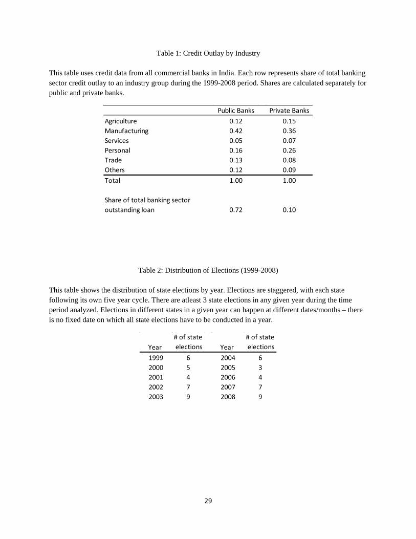
Table 1: Credit Outlay by Industry

This table uses credit data from all commercial banks in India. Each row represents share of total banking sector credit outlay to an industry group during the 1999-2008 period. Shares are calculated separately for public and private banks.

Table 2: Distribution of Elections (1999-2008)

This table shows the distribution of state elections by year. Elections are staggered, with each state following its own five year cycle. There are atleast 3 state elections in any given year during the time period analyzed. Elections in different states in a given year can happen at different dates/months – there is no fixed date on which all state elections have to be conducted in a year.

Public Banks Private BanksAgriculture 0.12 0.15Manufacturing 0.42 0.36Services 0.05 0.07Personal 0.16 0.26Trade 0.13 0.08Others 0.12 0.09Total 1.00 1.00

Share of total banking sector outstanding loan 0.72 0.10

Year # of state elections Year

# of state elections

1999 6 2004 62000 5 2005 32001 4 2006 42002 7 2007 72003 9 2008 9

29

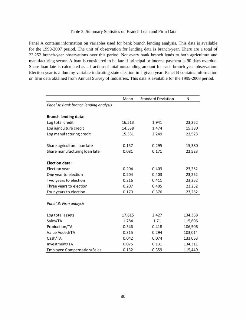
Table 3: Summary Statistics on Branch Loan and Firm Data

Panel A contains information on variables used for bank branch lending analysis. This data is available for the 1999-2007 period. The unit of observation for lending data is branch-year. There are a total of 23,252 branch-year observations over this period. Not every bank branch lends to both agriculture and manufacturing sector. A loan is considered to be late if principal or interest payment is 90 days overdue. Share loan late is calculated as a fraction of total outstanding amount for each branch-year observation. Election year is a dummy variable indicating state election in a given year. Panel B contains information on firm data obtained from Annual Survey of Industries. This data is available for the 1999-2008 period.

Mean Standard Deviation NPanel A: Bank branch lending analysis

Branch lending data:Log total credit 16.513 1.941 23,252 Log agriculture credit 14.538 1.474 15,380 Log manufacturing credit 15.531 2.249 22,523

Share agriculture loan late 0.157 0.295 15,380 Share manufacturing loan late 0.081 0.171 22,523

Election data:Election year 0.204 0.403 23,252 One year to election 0.204 0.403 23,252 Two years to election 0.216 0.411 23,252 Three years to election 0.207 0.405 23,252 Four years to election 0.170 0.376 23,252

Panel B: Firm analysis

Log total assets 17.815 2.427 134,368 Sales/TA 1.784 1.71 115,606 Production/TA 0.346 0.418 106,506 Value Added/TA 0.315 0.294 103,014 Cash/TA 0.042 0.074 133,063 Investment/TA 0.075 0.131 134,311 Employee Compensation/Sales 0.132 0.359 115,449

30

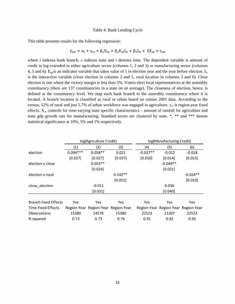
Table 4: Bank Lending Cycle

This table presents results for the following regression:

yist = αi + γrt + β1Est + β2EstIit + β3Iit + δXst + εist

where i indexes bank branch, s indexes state and t denotes time. The dependent variable is amount of credit in log extended to either agriculture sector (columns 1, 2 and 3) or manufacturing sector (columns 4, 5 and 6). Estis an indicator variable that takes value of 1 in election year and the year before election. Iit is the interaction variable (close election in columns 2 and 5, rural location in columns 3 and 6). Close election is one where the victory margin is less than 5%. Voters elect local representatives at the assembly constituency (there are 137 constituencies in a state on an average). The closeness of election, hence, is defined at the constituency level. We map each bank branch to the assembly constituency where it is located. A branch location is classified as rural or urban based on census 2001 data. According to the census, 52% of rural and just 5.7% of urban workforce was engaged in agriculture. γrt is region-year fixed effects. Xst controls for time-varying state specific characteristics – amount of rainfall for agriculture and state gdp growth rate for manufacturing. Standard errors are clustered by state. *, ** and *** denote statistical significance at 10%, 5% and 1% respectively.

(1) (2) (3) (4) (5) (6)election 0.094*** 0.058** 0.021 -0.027** -0.012 -0.018

[0.027] [0.027] [0.037] [0.010] [0.014] [0.013]election x close 0.053** -0.049**

[0.024] [0.021] election x rural 0.142** -0.024**

[0.051] [0.010]close_election -0.011 0.036

[0.031] [0.040]

Branch Fixed Effects Yes Yes Yes Yes Yes YesTime Fixed Effects Region-Year Region-Year Region-Year Region-Year Region-Year Region-YearObservations 15380 14578 15380 22523 21207 22523R-squared 0.73 0.73 0.74 0.91 0.92 0.92

log(Agriculture Credit) log(Manufacturing Credit)

31

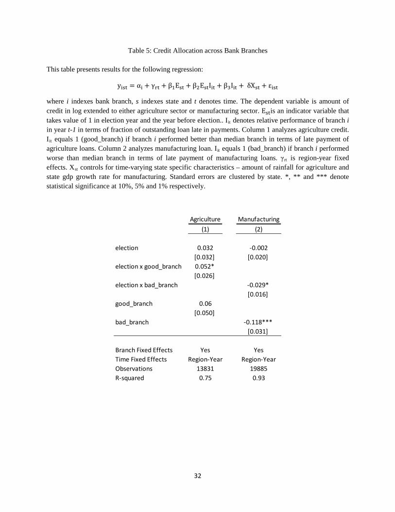
Table 5: Credit Allocation across Bank Branches

This table presents results for the following regression:

yist = αi + γrt + β1Est + β2EstIit + β3Iit + δXst + εist

where i indexes bank branch, s indexes state and t denotes time. The dependent variable is amount of credit in log extended to either agriculture sector or manufacturing sector. Estis an indicator variable that takes value of 1 in election year and the year before election.. Iit denotes relative performance of branch i in year t-1 in terms of fraction of outstanding loan late in payments. Column 1 analyzes agriculture credit. Iit equals 1 (good_branch) if branch i performed better than median branch in terms of late payment of agriculture loans. Column 2 analyzes manufacturing loan. Iit equals 1 (bad_branch) if branch i performed worse than median branch in terms of late payment of manufacturing loans. γrt is region-year fixed effects. Xst controls for time-varying state specific characteristics – amount of rainfall for agriculture and state gdp growth rate for manufacturing. Standard errors are clustered by state. *, ** and *** denote statistical significance at 10%, 5% and 1% respectively.

Agriculture Manufacturing(1) (2)

election 0.032 -0.002[0.032] [0.020]

election x good_branch 0.052* [0.026]

election x bad_branch -0.029* [0.016]

good_branch 0.06[0.050]

bad_branch -0.118*** [0.031]

Branch Fixed Effects Yes YesTime Fixed Effects Region-Year Region-YearObservations 13831 19885R-squared 0.75 0.93

32

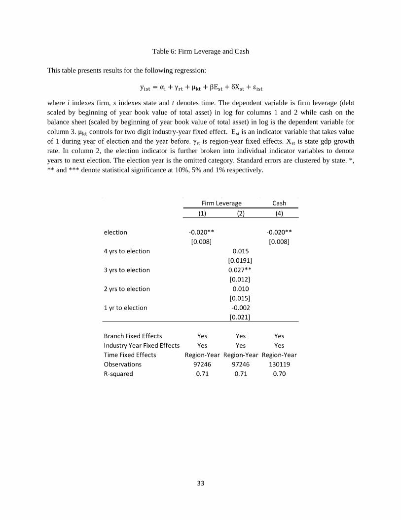
Table 6: Firm Leverage and Cash

This table presents results for the following regression:

yist = αi + γrt + µkt + βEst + δXst + εist

where i indexes firm, s indexes state and t denotes time. The dependent variable is firm leverage (debt scaled by beginning of year book value of total asset) in log for columns 1 and 2 while cash on the balance sheet (scaled by beginning of year book value of total asset) in log is the dependent variable for column 3. µkt controls for two digit industry-year fixed effect. Est is an indicator variable that takes value of 1 during year of election and the year before. γrt is region-year fixed effects. Xst is state gdp growth rate. In column 2, the election indicator is further broken into individual indicator variables to denote years to next election. The election year is the omitted category. Standard errors are clustered by state. *, ** and *** denote statistical significance at 10%, 5% and 1% respectively.

Cash(1) (2) (4)

election -0.020** -0.020**[0.008] [0.008]

4 yrs to election 0.015[0.0191]

3 yrs to election 0.027** [0.012]

2 yrs to election 0.010[0.015]

1 yr to election -0.002[0.021]

Branch Fixed Effects Yes Yes YesIndustry Year Fixed Effects Yes Yes YesTime Fixed Effects Region-Year Region-Year Region-YearObservations 97246 97246 130119R-squared 0.71 0.71 0.70

Firm Leverage

33

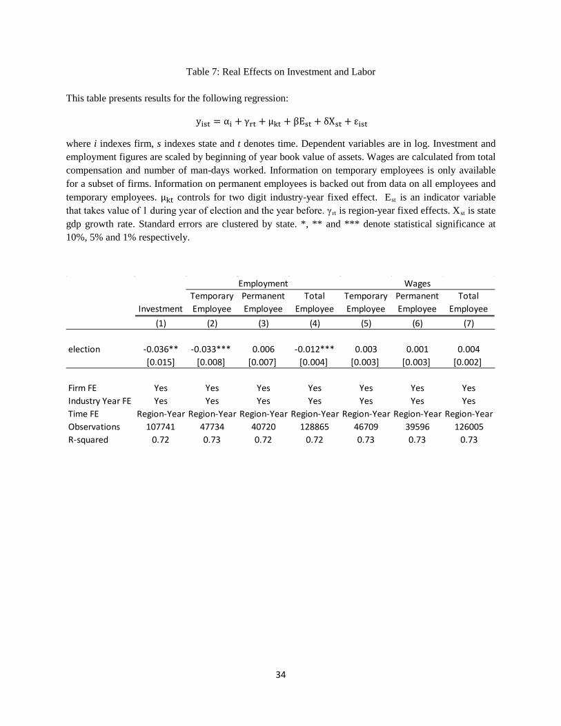
Table 7: Real Effects on Investment and Labor

This table presents results for the following regression:

yist = αi + γrt + µkt + βEst + δXst + εist

where i indexes firm, s indexes state and t denotes time. Dependent variables are in log. Investment and employment figures are scaled by beginning of year book value of assets. Wages are calculated from total compensation and number of man-days worked. Information on temporary employees is only available for a subset of firms. Information on permanent employees is backed out from data on all employees and temporary employees. µkt controls for two digit industry-year fixed effect. Est is an indicator variable that takes value of 1 during year of election and the year before. γrt is region-year fixed effects. Xst is state gdp growth rate. Standard errors are clustered by state. *, ** and *** denote statistical significance at 10%, 5% and 1% respectively.

InvestmentTemporary Employee

Permanent Employee

Total Employee

Temporary Employee

Permanent Employee

Total Employee

(1) (2) (3) (4) (5) (6) (7)

election -0.036** -0.033*** 0.006 -0.012*** 0.003 0.001 0.004[0.015] [0.008] [0.007] [0.004] [0.003] [0.003] [0.002]

Firm FE Yes Yes Yes Yes Yes Yes YesIndustry Year FE Yes Yes Yes Yes Yes Yes YesTime FE Region-Year Region-Year Region-Year Region-Year Region-Year Region-Year Region-YearObservations 107741 47734 40720 128865 46709 39596 126005R-squared 0.72 0.73 0.72 0.72 0.73 0.73 0.73

Employment Wages

34

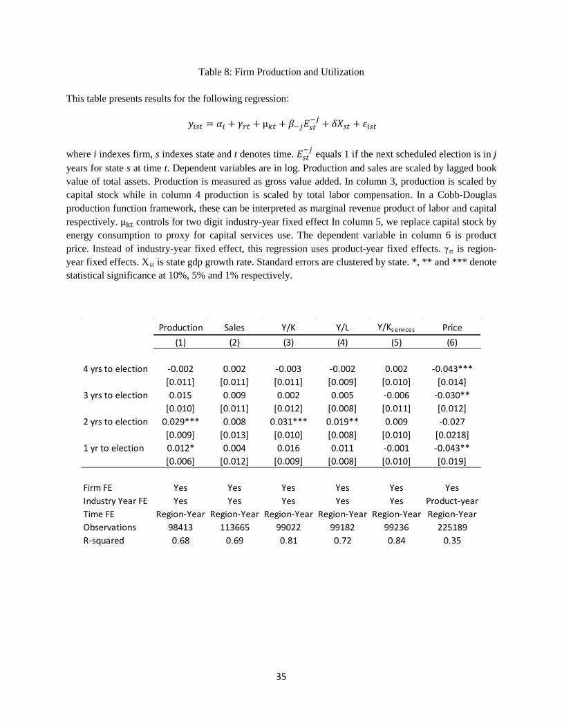
Table 8: Firm Production and Utilization

This table presents results for the following regression:

𝑦𝑦𝑖𝑖𝑖𝑖𝑖𝑖 = 𝛼𝛼𝑖𝑖 + 𝛾𝛾𝑟𝑟𝑖𝑖 + µ𝑘𝑘𝑖𝑖 + 𝛽𝛽−𝑗𝑗𝛽𝛽𝑖𝑖𝑖𝑖−𝑗𝑗 + 𝛿𝛿𝛿𝛿𝑖𝑖𝑖𝑖 + 𝜀𝜀𝑖𝑖𝑖𝑖𝑖𝑖

where i indexes firm, s indexes state and t denotes time. 𝛽𝛽𝑖𝑖𝑖𝑖−𝑗𝑗 equals 1 if the next scheduled election is in j

years for state s at time t. Dependent variables are in log. Production and sales are scaled by lagged book value of total assets. Production is measured as gross value added. In column 3, production is scaled by capital stock while in column 4 production is scaled by total labor compensation. In a Cobb-Douglas production function framework, these can be interpreted as marginal revenue product of labor and capital respectively. µkt controls for two digit industry-year fixed effect In column 5, we replace capital stock by energy consumption to proxy for capital services use. The dependent variable in column 6 is product price. Instead of industry-year fixed effect, this regression uses product-year fixed effects. γrt is region-year fixed effects. Xst is state gdp growth rate. Standard errors are clustered by state. *, ** and *** denote statistical significance at 10%, 5% and 1% respectively.

Production Sales Y/K Y/L Y/Kservices Price(1) (2) (3) (4) (5) (6)

4 yrs to election -0.002 0.002 -0.003 -0.002 0.002 -0.043***[0.011] [0.011] [0.011] [0.009] [0.010] [0.014]

3 yrs to election 0.015 0.009 0.002 0.005 -0.006 -0.030**[0.010] [0.011] [0.012] [0.008] [0.011] [0.012]

2 yrs to election 0.029*** 0.008 0.031*** 0.019** 0.009 -0.027[0.009] [0.013] [0.010] [0.008] [0.010] [0.0218]

1 yr to election 0.012* 0.004 0.016 0.011 -0.001 -0.043**[0.006] [0.012] [0.009] [0.008] [0.010] [0.019]

Firm FE Yes Yes Yes Yes Yes YesIndustry Year FE Yes Yes Yes Yes Yes Product-yearTime FE Region-Year Region-Year Region-Year Region-Year Region-Year Region-YearObservations 98413 113665 99022 99182 99236 225189R-squared 0.68 0.69 0.81 0.72 0.84 0.35

35

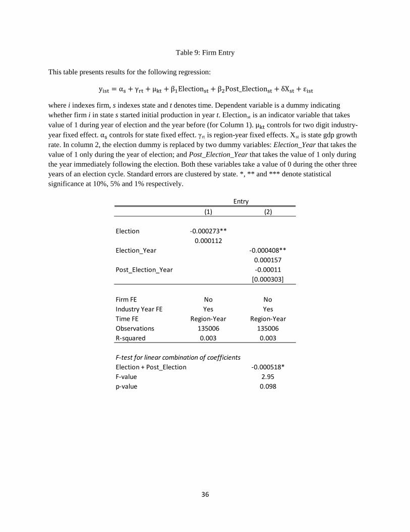
Table 9: Firm Entry

This table presents results for the following regression:

yist = αs + γrt + µkt + β1Electionst + β2Post_Electionst + δXst + εist

where i indexes firm, s indexes state and t denotes time. Dependent variable is a dummy indicating whether firm i in state s started initial production in year t. Electionst is an indicator variable that takes value of 1 during year of election and the year before (for Column 1). µkt controls for two digit industry-year fixed effect. αs controls for state fixed effect. γrt is region-year fixed effects. Xst is state gdp growth rate. In column 2, the election dummy is replaced by two dummy variables: Election_Year that takes the value of 1 only during the year of election; and Post_Election_Year that takes the value of 1 only during the year immediately following the election. Both these variables take a value of 0 during the other three years of an election cycle. Standard errors are clustered by state. *, ** and *** denote statistical significance at 10%, 5% and 1% respectively.

(1) (2)

Election -0.000273**0.000112

Election_Year -0.000408**0.000157

Post_Election_Year -0.00011[0.000303]

Firm FE No NoIndustry Year FE Yes YesTime FE Region-Year Region-YearObservations 135006 135006R-squared 0.003 0.003

F-test for linear combination of coefficientsElection + Post_Election -0.000518*F-value 2.95p-value 0.098

Entry

36

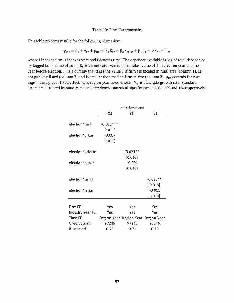
Table 10: Firm Heterogeneity

This table presents results for the following regression:

yist = αi + γrt + µkt + β1Est + β2EstIit + β3Iit + δXst + εist

where i indexes firm, s indexes state and t denotes time. The dependent variable is log of total debt scaled by lagged book value of asset. Estis an indicator variable that takes value of 1 in election year and the year before election. Iit is a dummy that takes the value 1 if firm i is located in rural area (column 1), is not publicly listed (column 2) and is smaller than median firm in size (column 3). µkt controls for two digit industry-year fixed effect. γrt is region-year fixed effects. Xst is state gdp growth rate. Standard errors are clustered by state. *, ** and *** denote statistical significance at 10%, 5% and 1% respectively.

(1) (2) (3)

election*rural -0.031*** [0.011]

election*urban -0.007[0.011]

election*private -0.023** [0.010]

election*public -0.004[0.010]

election*small -0.030** [0.013]

election*large -0.011[0.010]

Firm FE Yes Yes YesIndustry Year FE Yes Yes YesTime FE Region-Year Region-Year Region-YearObservations 97246 97246 97246R-squared 0.71 0.71 0.72

Firm Leverage

37

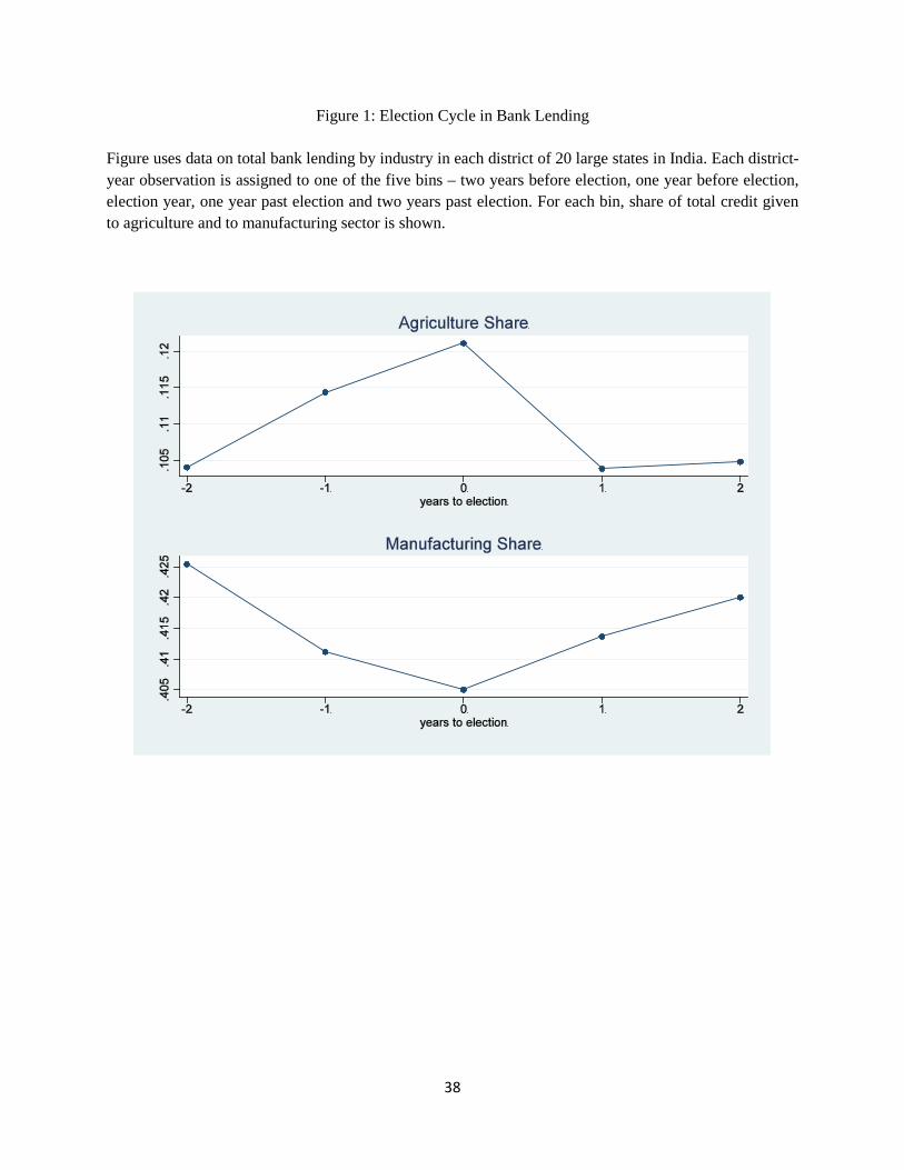
Figure 1: Election Cycle in Bank Lending

Figure uses data on total bank lending by industry in each district of 20 large states in India. Each district-year observation is assigned to one of the five bins – two years before election, one year before election, election year, one year past election and two years past election. For each bin, share of total credit given to agriculture and to manufacturing sector is shown.

38

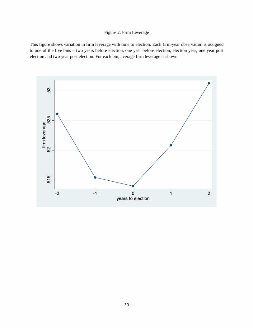
Figure 2: Firm Leverage

This figure shows variation in firm leverage with time to election. Each firm-year observation is assigned to one of the five bins – two years before election, one year before election, election year, one year post election and two year post election. For each bin, average firm leverage is shown.

39

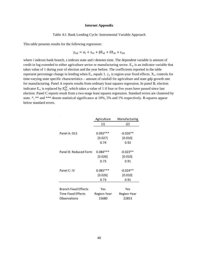
Internet Appendix

Table A1: Bank Lending Cycle: Instrumental Variable Approach

This table presents results for the following regression:

yist = αi + γrt + βEst + δXst + εist

where i indexes bank branch, s indexes state and t denotes time. The dependent variable is amount of credit in log extended to either agriculture sector or manufacturing sector. Est is an indicator variable that takes value of 1 during year of election and the year before. The coefficients reported in the table represent percentage change in lending when Est equals 1. γrt is region-year fixed effects. Xst controls for time-varying state specific characteristics – amount of rainfall for agriculture and state gdp growth rate for manufacturing. Panel A reports results from ordinary least squares regression. In panel B, election indicator Est is replaced by EstIV, which takes a value of 1 if four or five years have passed since last election. Panel C reports result from a two-stage least squares regression. Standard errors are clustered by state. *, ** and *** denote statistical significance at 10%, 5% and 1% respectively. R-squares appear below standard errors.

Agriculture Manufacturing(1) (2)

Panel A: OLS 0.092*** -0.026** [0.027] [0.010]

0.74 0.92

Panel B: Reduced Form 0.084*** -0.023** [0.026] [0.010]

0.73 0.91

Panel C: IV 0.085*** -0.024** [0.026] [0.010]

0.73 0.91

Branch Fixed Effects Yes YesTime Fixed Effects Region-Year Region-YearObservations 15680 22853

40

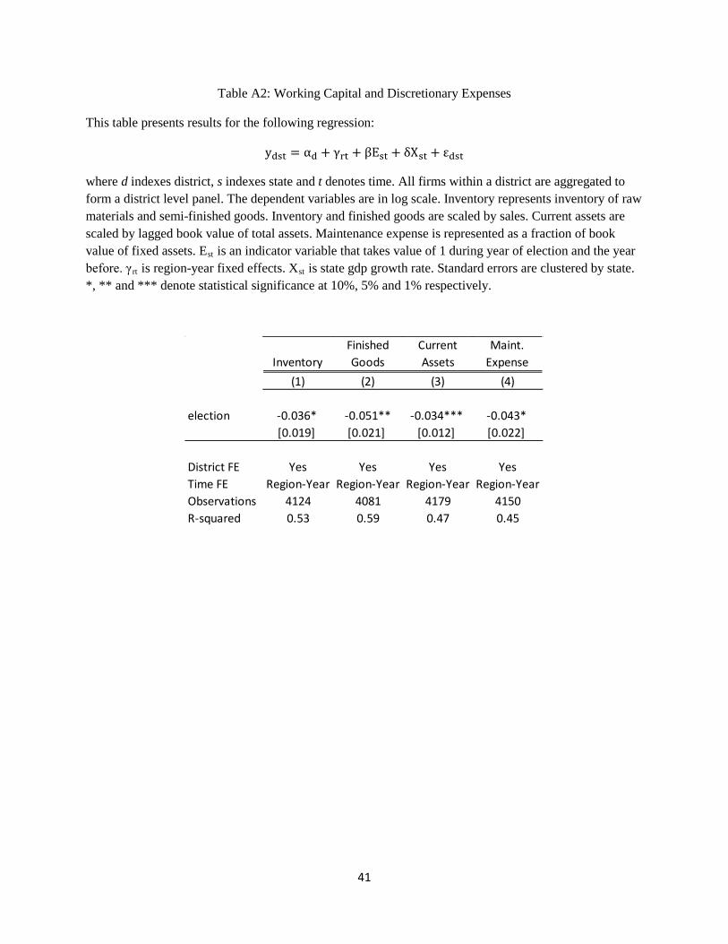
Table A2: Working Capital and Discretionary Expenses

This table presents results for the following regression:

ydst = αd + γrt + βEst + δXst + εdst

where d indexes district, s indexes state and t denotes time. All firms within a district are aggregated to form a district level panel. The dependent variables are in log scale. Inventory represents inventory of raw materials and semi-finished goods. Inventory and finished goods are scaled by sales. Current assets are scaled by lagged book value of total assets. Maintenance expense is represented as a fraction of book value of fixed assets. Est is an indicator variable that takes value of 1 during year of election and the year before. γrt is region-year fixed effects. Xst is state gdp growth rate. Standard errors are clustered by state. *, ** and *** denote statistical significance at 10%, 5% and 1% respectively.

InventoryFinished Goods

Current Assets

Maint. Expense

(1) (2) (3) (4)

election -0.036* -0.051** -0.034*** -0.043* [0.019] [0.021] [0.012] [0.022]

District FE Yes Yes Yes YesTime FE Region-Year Region-Year Region-Year Region-YearObservations 4124 4081 4179 4150R-squared 0.53 0.59 0.47 0.45

41