Content Page

NO PARTICULARS PAGE

1 Top Glove to boost nitrile gloves output 2-11

2 Honda: Car prices to fall post- GST 12-20

3 A $15- hour minimum wage could harm America’s poorest workers

21-28

4 Corn yields up, prices down 29-38

5 Hadrian the robot bricklayer can build a whole house in two days

39-45

6 Fast food chain’s explosive offering to suit local taste buds 46-53

7 FAO urges sustainability over immediate profits to safeguard water supplies

54-60

8 Appendix and References 61

1

2

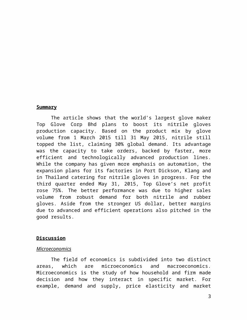
Summary

The article shows that the world’s largest glove maker Top Glove Corp Bhd plans to boost its nitrile gloves production capacity. Based on the product mix by glove volume from 1 March 2015 till 31 May 2015, nitrile still topped the list, claiming 30% global demand. Its advantage was the capacity to take orders, backed by faster, more efficient and technologically advanced production lines. While the company has given more emphasis on automation, the expansion plans for its factories in Port Dickson, Klang and in Thailand catering for nitrile gloves in progress. For the third quarter ended May 31, 2015, Top Glove’s net profit rose 75%. The better performance was due to higher sales volume from robust demand for both nitrile and rubber gloves. Aside from the stronger US dollar, better margins due to advanced and efficient operations also pitched in the good results.

Discussion

Microeconomics

The field of economics is subdivided into two distinct areas, which are microeconomics and macroeconomics. Microeconomics is the study of how household and firm made decision and how they interact in specific market. For example, demand and supply, price elasticity and market structure. However, macroeconomics is the study of economy –wide phenomena, including inflation, unemployment and economic growth.

Market Structure

The model of monopolistic competition defines a common market structure in which firms have many competitors, but each firm sells a slightly different product. Top Glove is categorized as monopolistic competition firm. Monopolistic competition markets reveal the following characteristics:

1. Large Number of Small Firms

Monopolistic competition market contains a large number of small firms, each firm which is relatively small compared to the overall size of the market. This ensures that all firms are relatively competitive with very little market control over price or quantity. In particular, each firm consists of hundreds or even thousands competitors. The size of capital of these firms are small.

2. Relatively to Enter or Exit the Market

Most firms involved in monopolistic competition market have low capital requirements, firms can easily enter or exit the market. However, the amount of investment is generally larger than for perfect competition market, since there is

3

an expense to developing or introducing their differentiated products and for doing many advertisement. With easy entry and exit, firms will enter a market when the present firms are earning an economic profit and will exit the market when the firms are making an economic loss. Therefore, this market allows the remaining market earning a zero economic profit in the long run.

3. Differentiated Product

Monopolistic competition market cannot exist unless there is a slightly difference among the product that is produced by each firm, which results from differences in product quality, location, service, and advertising. The products produced are not similar and identical products. Product quality can differ in function, design, inputs, and workmanship.

4. Price Maker

Firms are price makers and are faced with a downward sloping demand curve. This is because each firm makes a differentiated product, therefore it can charge a higher or lower price than its competitors. The firm can set its own price and does not have to take the price from the market. This also means that the demand curve will downwards sloping.

5. Brand Names and Do Advertisement

Brand names will serve to distinguish identical or nearly identical products and to increase the value of advertising in that the brand name serves as an object to which desirable characteristics can be attached. Advertising is used to build brand awareness or loyalty to a particular consumer.

6. In the Short Run

A monopolistic competition firm maximizes economic profit or minimizes economies losses by producing the quantity that corresponds to when marginal revenue (MR) equals marginal cost (MC). If average total cost (ATC) is below the market price, then the firm will earn an economic profit. However, if the average total cost (ATC) is above the market price, then the firm will experience an economic loss.

7. In the Long Run

If the monopolistic competition firms in a market are earning an economic profit, then it will attract other firms enter the same market, which will reduce the profits of the other firms. More firms will continue to enter the market until the firms are earning on a zero economic profit. However, if there are too many firms in the market, then firms will start to make a loss, which will cause them to exit the market. Consequently, the remaining firms will return to normal profitability.

4

Hence, the long-run equilibrium for monopolistic competition market will compare the market price to the average total cost, where marginal revenue equals marginal cost.

Cost of Production

Top Glove has manufactured various types of glove in the market. The firm is large and needs to employ thousands of workers. Besides, the firm has thousands of stockholders who share in the firms’ profits. Each firm’s objective is to maximize their profits as large as possible. Firms incur costs when they buy inputs to produce the goods and services that they plan to sell. We can derive several related measures of cost, which will turn out to be useful when we analyze the production of outputs.

Total Fixed Costs

Total fixed costs (TFC) are constant as output increases, the curve is a horizontal line on the cost graph. Fixed costs are those costs over which a firm has no control. They are usually tied to fixed inputs or resources. The fixed costs must be paid, otherwise the firm may have to shut down. For example, Top Glove’s fixed costs include any rent for warehouse and others. Similarly, Top Glove needs to hire many full-time employees to produce the gloves.

Total Variable Costs

The total variable cost(TVC) curve slopes up at an accelerating rate, reflecting the law of diminishing marginal returns. Variable costs are those costs which a firm can change at will. They relate to inputs or resources which are not fixed.For instance, Top Glove has hire more workers to make more gloves. Top Glove has to pay them wages. The wages paid for them are variable costs.

Total Costs

The total cost (TC) curve is found by adding total fixed costs and total variable costs. The total cost curve is represented an upwards sloping curve graphically: costs increase as output increases. The curve is generally S shaped, reflecting the increasing efficiency starting from a low level of production, and then a decreasing efficiency as the volume of production goes beyond the point of diminishing returns.

Average Fixed Costs

Average fixed costs (AFC) are found by dividing total fixed costs by output. As fixed cost is divided by an increasing output, average fixed costs will continue to fall.

Average Variable Costs

5

Average variable cost (AVC) is calculated by dividing total variable cost by quantity produced. It will reflect an increasing then decreasing efficiency in production as output changes.

Average Total Cost

Average total cost (ATC) is calculated by dividing total cost by the quantity produced. It can also be obtained by adding up average fixed cost and average variable cost at each level of production. The average total cost curve is represented a steep decreasing portion and a slightly increasing portion. These are attributable to the fixed and variable cost arrangements.

Marginal Cost

Marginal cost (MC) is calculated by dividing the change in total cost by the change in quantity. The marginal cost curve reflectsan increasing then decreasing efficiency as output increases. For example, the marginal, or additional, cost per unit changes more than the average total cost for each unit. The cost of one additional meal start to increase before average total cost does.

6

Analysis

Market Structure

Top Glove is considered as monopolistic competition market because when consumers can find that there are many brands of gloves available in the shop. Besides, there are many sellers competing for the same group of consumers. Top Glove produces the glove that is at least slightly different from the other firms. The sellers in this market are price makers rather than price takers, therefore Top Glove faces a downward sloping demand curve.Furthermore, the demand curve is downward sloping because glove is considered as a necessity product, so it is elastic and has many close substitutes products in the market.

Moreover, the firms can enter or exit the market easily without restriction. Thus, the number of firms in the market can be adjustfrom an economic profit to a zero economic profit or from an economic loss to a zero economic profit in the long run. A monopolistically competitive market departs from the perfectly competitive ideal because each of the sellers offers a slightly different product.

The monopolistically competitive firm follows a monopolist’s rule for profit maximization: It chooses the profit-maximizing output at which marginal revenue equals marginal cost and then uses the demand curve to find the market price reliable with the quantity.

In the short-run, Top Glove will maximize profit by producing the quantity at which marginal revenue equals marginal costs. Top Glove in Figure 1.1 makes an economic profit because, at this quantity, price is above average total cost. However, when there is a short-run economic profit, it will attract new firms to enter the market. This will increase the number of glove products supplied or offered by the other firms. Top Glove will face a decreasing demand of glove in the market. Therefore, incumbent firms’ demand curves will shift to the left. As the demand of glove products decrease, thus Top Glove and the other firms’ profit will be declined.

7

Quantityof Glove

D=AR=PMR

ATC

MC

ECONOMIC PROFIT

Priceof Glove

P

ATC

Profit-maximizing Quantity

0

MC

ECONOMIC LOSS

MR

ATCATC

D=AR=P

P

Quantityof Glove

Priceof Glove

Loss-minimizing Quantity0

Figure 1.1: Top Glove Makes Economics Profit in Short Run

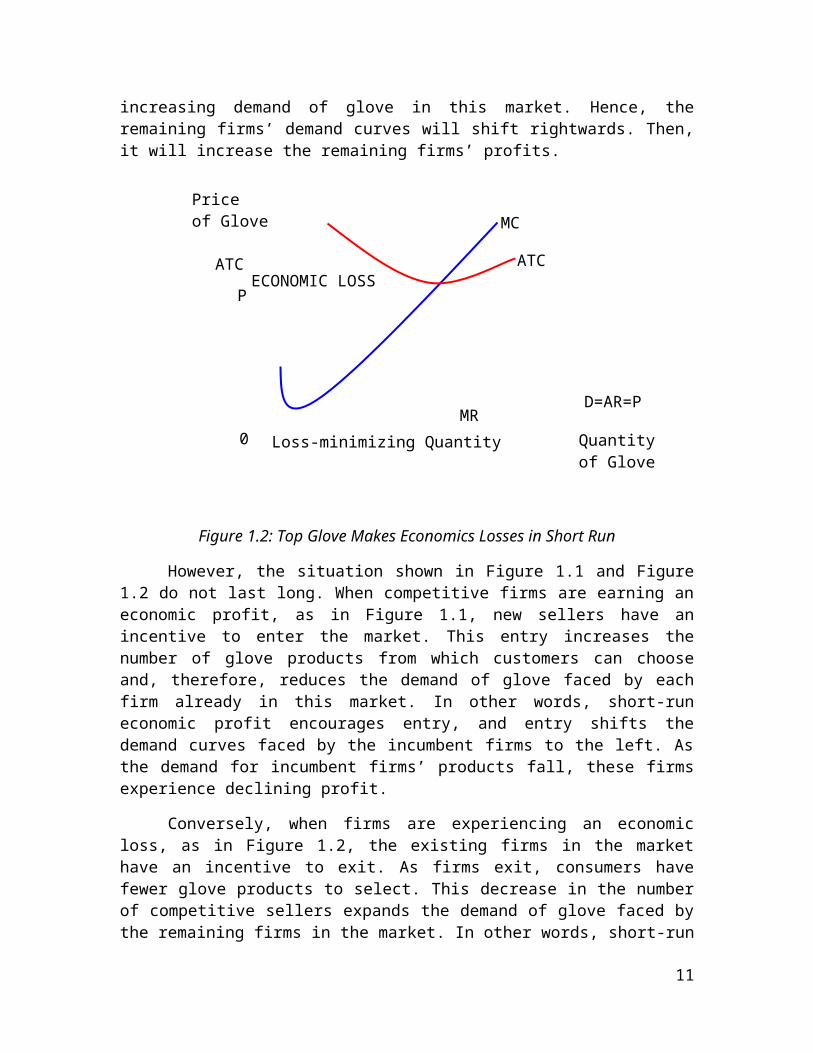
Furthermore, in the short-run Top Glove in Figure 1.2 makes an economic loss because, at this quantityat which marginal revenue equals marginal costs, price is less than average total cost. Thus, short-run economic losses encourage the existing firms to leave the market. It will reduce the number of output of glove products supplied or offered by the firms. The remaining firms will face an increasing demand of glove in this market. Hence, the remaining firms’ demand curves will shift rightwards. Then, it will increase the remaining firms’ profits.

Figure 1.2: Top Glove Makes Economics Losses in Short Run

8

Profit-maximizingQuantity

D=AR=P

MC

ATC

P=ATC

MR

0 Quantityof Glove

Priceof Glove

However, the situation shown in Figure 1.1 and Figure 1.2 do not last long. When competitive firms are earning an economic profit, as in Figure 1.1, new sellers have an incentive to enter the market. This entry increases the number of glove products from which customers can choose and, therefore, reduces the demand of glove faced by each firm already in this market. In other words, short-run economic profit encourages entry, and entry shifts the demand curves faced by the incumbent firms to the left. As the demand for incumbent firms’ products fall, these firms experience declining profit.

Conversely, when firms are experiencing an economic loss, as in Figure 1.2, the existing firms in the market have an incentive to exit. As firms exit, consumers have fewer glove products to select. This decrease in the number of competitive sellers expands the demand of glove faced by the remaining firms in the market. In other words, short-run economic losses encourage exit, and exit shifts the demand curves of the remaining firms to the right. As the demand for the remaining firms’ glove products rises, these firms experience rising profit or declining losses.

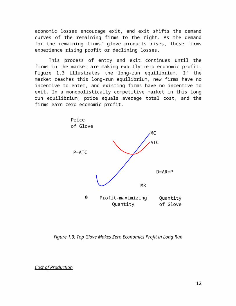
This process of entry and exit continues until the firms in the market are making exactly zero economic profit. Figure 1.3 illustrates the long-run equilibrium. If the market reaches this long-run equilibrium, new firms have no incentive to enter, and existing firms have no incentive to exit. In a monopolistically competitive market in this long run equilibrium, price equals average total cost, and the firms earn zero economic profit.

Figure 1.3: Top Glove Makes Zero Economics Profit in Long Run

9

Cost of Production

Economy is made up of thousands of firms that produce goods and services for consumer enjoy every day. For example, Top Glove produces various types of gloves. Top Glove needs to employ thousands of workers to produce these types of gloves. Besides, according to the law of supply, most firms are willing to produce and sell a larger quantity of a good when the price is higher, and this response leads to a supply curve that upwards sloping.

Using technology to produce goods can make tasks more efficiency. Therefore, Top Glove has started to use the technology to produce gloves, and it makes the production lines more efficient, faster, easier and at a low cost. This advancement on technology has a great impact on short-run curves by when technology improves then production of gloves will increase. As the production of gloves increase which causes the average variable cost decrease. Besides, when the production of gloves increase, the fixed cost is spread over more output, causing the average fixed cost to decrease. For instance, the fixed costs which isincluded rental payments, salaries for full-time employees, monthly equipment fees and structured loan payments. Top Glove has given more emphasis on the automation in production line causes the average of variable cost decreases. The variable costs involved the wages for workers, utility fees, and costs of raw materials. Because of the automation in production line which is used by Top Glove, the labour in Top Glove will be replaced by the technology. By improvingthe technology, Top Glove will only hire fewer workers or employeesand will increase more production of glove on average. Therefore, the amount of wages paid and time required for producing gloves decrease, which will decrease the average variable cost.

Moreover, Top Glove will finally reach the point where there is the advancement of technology can be produced. Therefore, productivity of Top Glove will rise to a maximum possible output. Furthermore, human will try to improve or introduce new technology for producing the glove in the future. Human would come up with latest technology and change the technology become more efficient, faster and save costs. Figure 1.3 shown that the technology came to the singularity. The singularity is meant technological change so rapid and so profound that it represents a rupture in the fabric of human history. Hence, Top Glove will face the singularity problem in the future in the production line for producing gloves.

10

Time

Singularity

TechnologicalProgress

Figure 1.4: Technology Advancement for Top Glove in the Future

Conclusion

In conclusion, Top Glove is a monopolistic competition firm because there are many sellers and they can enter or exit the market easily. Furthermore, the advancement of the technology makes the production easier, faster by using a low cost and increase the quantity of outputs.

11

12

Summary

Honda Malaysia SdnBhd expects its vehicles prices to be reduced between 1% and 2% on average, after the implementation of Goods and Services Tax (GST) in April this year. This is due to the proposed GST rate of 6% is lower than the current 10% of Sales and Service Tax (SST). CEO Yoichiro Ueno is targeting 85,000 sales units this year and said that the drop of the car prices is expected for almost of its models, depending on each model as the SST is different for each car. Last year, the group has exceeded its 76, 000 units sales target, where it achieved 77, 485 units, translated to an increase in market share to 11.6% against 2014 TIV of 667, 000 units.

Discussion

Price Elasticity of Demand and Its Determinants

The law of demand states that a fall in the price of a good, and it will affect the quantity demanded to rise. The price elasticity of demand measures how much the quantity demanded responds to a change in price. If the quantity demanded responds substantially to changes in the price, demand for a good is elastic.Whereas the demands is inelastic, when the quantity responds only slightly to changes in price.

The determinant of price elasticity of demand is availability of close substitutes. Good with close substitutes tend to have more elastic demand. Whereas good with no close substitutes or few substitutes tend to have less elastic demand. Beside, we can determine the price elasticity of demand based on the time horizon. In long run, the price elasticity of demand is inelastic. This is because consumers can take time to adjust their arrangement toward the articular goods if the price of goods decrease or increase. However, in short run, the price elasticity of demand is inelastic because the consumers have not enough time to do their adjustment. Furthermore, price elasticity of demand can be determined based on the necessities versus luxuries. Necessities tend to have inelastic demand. For example, if the price of rice increases, consumers still will go and buy as usual because this is necessary goods for them. Whereas luxury goods tend to have elastic demand and consumers will have highly responsive if the price of luxury goods increase or decrease.

The Costs of Taxation

Taxes are imposed by government to raise revenue, and that revenue must come out of someone’s pocket. Both buyers and sellers are worse off when a good is taxed: A tax raises the price buyer paid and lower the price seller received.

Deadweight loss is a loss of economic efficiency caused by an inefficient allocation of resources. It does not matter whether a tax on a good is levied on buyer of seller of the good. When a tax is levied on buyer, the demand curve will shift downward by the size of the tax. Besides,when it is levied on seller, the supply curve will shift upward by the amount. In case, when the tax is imposed, the price paid by buyer raises, and the price received by seller falls. In the end, buyer and seller share the burden of tax, regardless of how it is levied.

13

Market Structure (Oligopoly)

There are four types of market structures which are included perfect competition, monopoly, monopolistic competition and oligopoly. An oligopoly market has a few characteristic which included:

1. Mutual Interdependence

Mutual interdependence exists when the actions of one firm has a major impact on the other firms in the industry. Mutual interdependence exists within an oligopoly industry because each of the oligopolists has a sizable part of the market. As a consequence, when it changes its sales, its prices, or its marketing strategies, this oligopoly firm will likely affect the sales of other firms within the industry.

2. Many Barriers of Market Entry and Exit

Barriers to entry are the key characteristic that separates oligopoly from monopolistic competition on the continuum of market structures. This is because with substantial entry barriers found in oligopoly, firms cannot enter the industry as easily. The most noted entry barriers are exclusive resource ownership, patents and copyrights, other government restrictions, and high start-up cost.

3. Products

Oligopolistic industries general come in two varieties which are identical product oligopoly and differentiated product oligopoly. Identical product oligopoly tends to process raw materials or produce intermediate goods that are used as inputs such as petroleum. While different product oligopoly focuses on the goods that are mainly foe personal consumption because different people have difference wants and needs. The example of differentiated product oligopoly included computer and automobile.

14

Price of Honda

P1

P0

Q1Q0 QuantityOf Honda

DD

Analysis

Price Elasticity of Demand

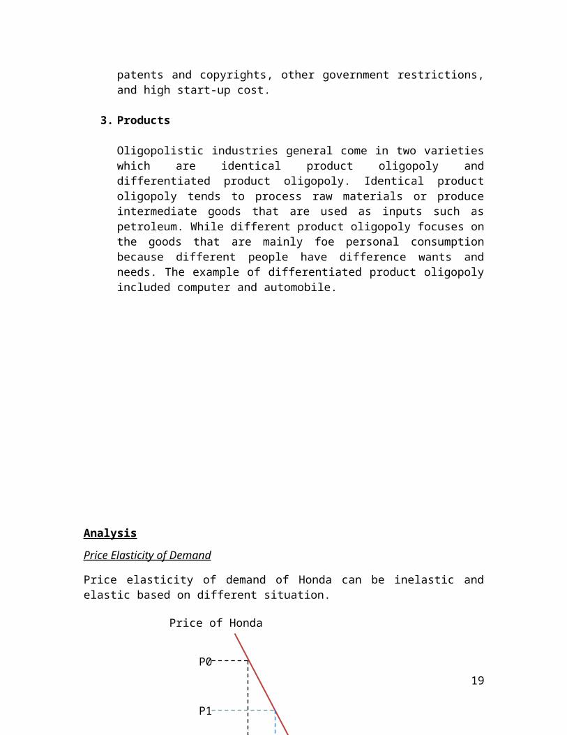
Price elasticity of demand of Honda can be inelastic and elastic based on different situation.

Figure 2.1: Price Inelastic for Honda

An inelastic graph is a situation when demand for an item changes proportionately less than the price changes, then the item is price inelastic. From the article, we can conclude that the price of Honda has decrease at least 4% from its original price due to the changing of Sales and Service Tax which is 10% change to Goods and Services Tax, GST which is 6%. The price elasticity of demand would be different based on different consumer. For example, the consumers who are working and has a stable income, the price elasticity of demand for this type of consumer is inelastic. Therefore, according to the Figure 2.1, when the price of Honda decreases from P0 to P1, the quantity demanded of Honda has slightly increases from Q0 to Q1. This can be proved that this type of consumers is less sensitive towards a decrease price of Honda. This is because consumers who are working, have a higher purchasing power. Hence, decrease in price of Honda will not give high effect to these consumers.

Another factor for Honda to be inelastic is because the availability of close substitutes. Honda is the product that has few close substitute and a less competitive market. Therefore, consumer would not easily switch from buying Honda cars to buying from other car manufacturers.

Moreover, Honda will be considered as price inelastic because Honda is mutually interdependence. Firms that are interdependent cannot act independently of each other. A firm that operates in a market with just a few competitors must take the potential reaction of its closest rivals into account when making its own decisions. For example, if Honda

15

Quantityof HondaQ3 Q4

P3

P4

Price of Honda

DD

wishes to increase its market share by reducing price, it must take into account the possibility that close rivals, such as Toyota and Kia, may reduce their price in relation. Therefore other automobile company will also reduce their price when Honda reduces their price. Since Honda is under non price competition, consumer will not consider much on the price because the prices of automobiles that have the similar specializations from different firms are almost same. From Figure 2.1, this clearly shows that under mutually interdependence, Honda is inelastic as people are not sensitive to the price and the change in price of Honda (decreases from P0 to P1) is greater than the change in demand for Honda (increases from Q0 to Q1

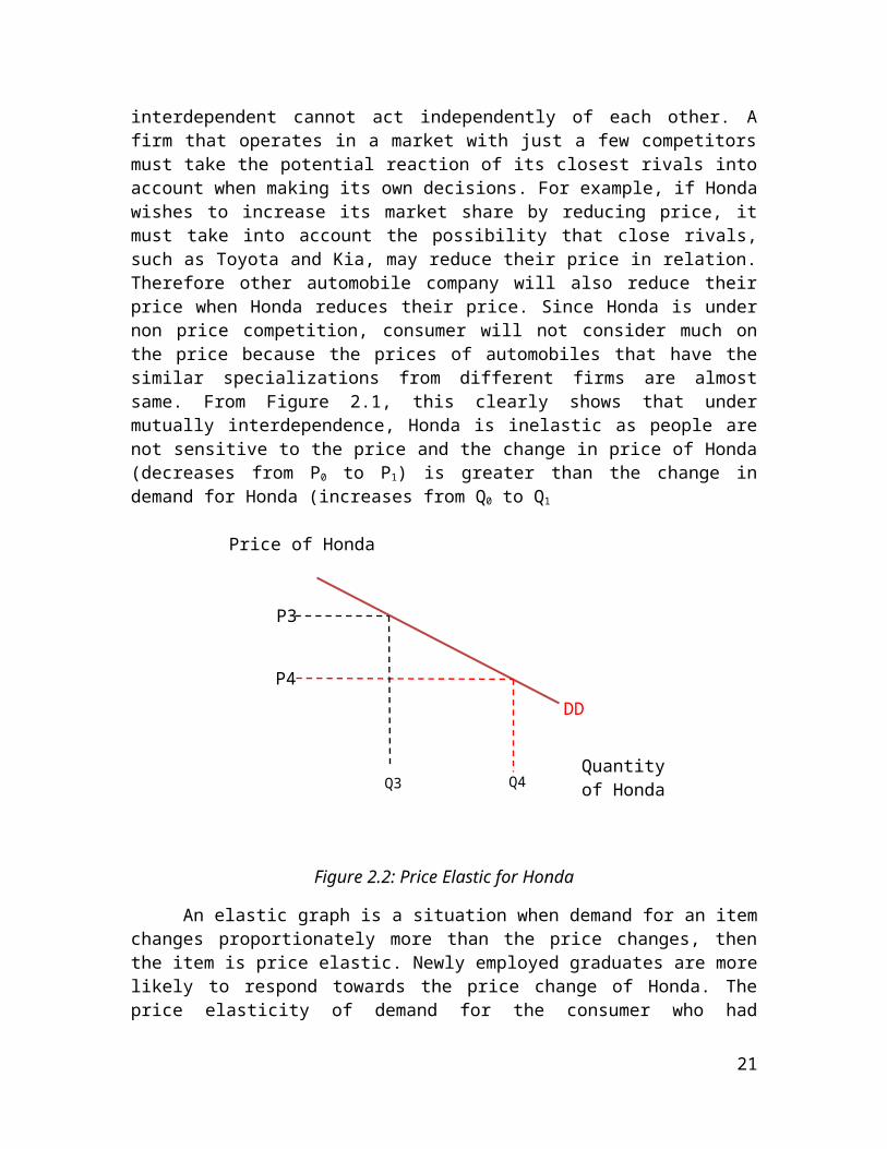
Figure 2.2: Price Elastic for Honda

An elastic graph is a situation when demand for an item changes proportionately more than the price changes, then the item is price elastic. Newly employed graduates are more likely to respond towards the price change of Honda. The price elasticity of demand for the consumer who had graduated and just started workingis elastic. According to Figure 2.2, we can see that the demand curve is flatter as it shows that the elastic demand. This is because the flatter demand that passes through a given point, the greater the price elasticity of demand. Therefore, from the Figure 2.2, when the price of Honda decreases from P3 to P4, the quantity demanded of Honda has increases gradually from Q3 to Q4. The increase of quantity demanded of Honda in elastic demand (Figure2.2) is more than the quantity demanded of Honda in inelastic demand (Figure 2.1).This proves that this type of consumers is highly sensitive towards a slight decrease in price of Honda. This is because newly employed graduates have lower purchasing power. Hence, the decrease in price of Honda will give higher effect to this group of consumers.Besides, Honda is considered as a luxury good for a newly employed graduated. Therefore, when the price of Honda decreases, newly employed graduated will tend to buy Honda since the quality of Honda is recognized. Therefore, it has slightly increased the sales of Honda in order to achieve the sales target that had stated on the article.

Moreover, when the government has just imposed the GST of 6%, the price of Honda will not change because in short term consumer would not have enough time to

16

PS

P

PB

B

A

SS

DD

Price of Honda

Quantity of Honda

adjust to the price change or they have not acknowledge the price change in Honda cars. While in long term they would have the time to choose and compare the price of Honda cars with other automobile firms. Although when the price of Honda cars decreases, other firm would also decrease the price due to the GST implemented but those who are “Honda fans” would opt for Honda cars because consumer goes for a car with better quality, design and functions. Logically thinking fresh graduates buy car to use for long term, they would not want to change car every year. Therefore, they will go for a car which is high in quality and another plus point will be now they would be able to afford for a Honda car.

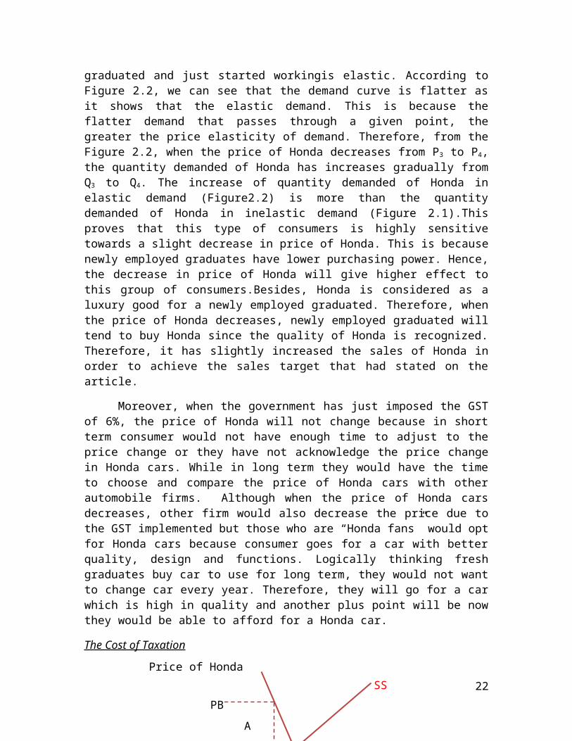
The Cost of Taxation

Figure 2.3: Inelastic Demand and Elastic Supply

Besides, for both buyers and sellers of Honda, they need to bear different amount burden of tax. For example, according to Figure 2.3, buyers will bear higher amount burden of tax. However, the burdens of tax depend on the elasticity of demand and supply. For the consumers who are still working and have a stable income, it has inelastic demand and elastic supply. This also means that the sellers of Honda are very responsive to the changes in the price of Honda, whereas the buyers of Honda are not responsive to the price of Honda. When a GST of 6% is imposed by the government on Honda with these elasticities, the price received by sellers does not fall much, so sellers of Honda will only bear a small amount burden of tax where is the area of B in the Figure 2.3. By contrast, the price paid by the buyers who purchase Honda rises substantially. This mean that buyers who purchase Honda bear most of the burden of the tax where is the area of A in the Figure 2.3.

17

PS

PBC

D

SS

P

Price of Honda

Quantity of Honda

DD

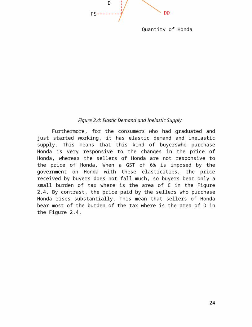
Figure 2.4: Elastic Demand and Inelastic Supply

Furthermore, for the consumers who had graduated and just started working, it has elastic demand and inelastic supply. This means that this kind of buyerswho purchase Honda is very responsive to the changes in the price of Honda, whereas the sellers of Honda are not responsive to the price of Honda. When a GST of 6% is imposed by the government on Honda with these elasticities, the price received by buyers does not fall much, so buyers bear only a small burden of tax where is the area of C in the Figure 2.4. By contrast, the price paid by the sellers who purchase Honda rises substantially. This mean that sellers of Honda bear most of the burden of the tax where is the area of D in the Figure 2.4.

18

Market Structure

Honda car’s market structure is categorized under oligopoly market. One of the characteristics of oligopoly is many market barriers of market entry and exit. Due to government restrictions, Honda Company has its own copyright given by the government and Honda has their own patent issues. Besides, Honda is now become a mature and has successfully reached economies of scale. Before Honda becomes one of the automobile industries in Malaysia, Honda had already gone through brand name recognition by the government. Honda is capable to reach the start-up cost to start up their company. If a new firm tries to enter the automobile market they would have to go through what Honda had went through if they fail to do so, they will fail to enter the market.

Moreover, Honda is a differentiated product oligopoly. Honda’s products seem different from other companies but the engines or functions of their products can be same. The technology that uses to produce a car compare to other industries is different. Firms have designed many patterns for the car, the main purpose is to attract customers to buy their products. In addition, the patents and ways to produce have to be different from other industry. Besides, they have their own copyrights and name recognition. This is why Honda which is in oligopoly market is homogenous and can be differentiated at the same time.

Furthermore, Honda had been characterized by a small number of competitors and usually non-price competition because it just has few suppliers. Honda which is oligopolistic firm keeps a close eye on the activities of other firms such as Toyota, Kia, and Mitsubishi in the industry. Decisions made by Honda invariably affect others and are invariably affected by others where each Honda seller is aware of the others actions, and where these actions effect the decisions of the other sellers. When Honda’s price decreases, the other competitors will also decrease their price and will not have conflict in the price competition.

19

Q1 Quantity of Honda

MR2

P1

MC2

MC1D1

D2

MR1

Price of Honda

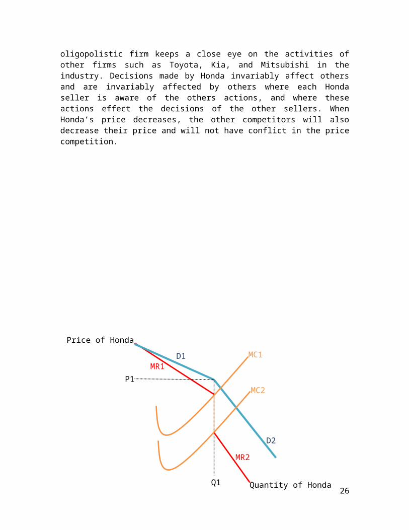
Figure 2.5: Oligopoly Market for Honda

Figure 2.5 showsthat the oligopoly market for Honda. P1 is the price of Honda and the Q1 is the quantity of Honda. From the Figure 2.5, we can conclude that if Honda raises its price (D1), others manufactured cars do not follow the increase, then revenue will decline in spite of the price increase. If Honda lowers its price (D2), then the other firm will match the decrease to avoid losing market share. This is because there is a gap in the marginal revenue curve (MR1- MR2). Since Honda maximizes profit by producing that quantity where marginal cost equals marginal revenue, Honda will not change the price of their product as long as the marginal cost is between MC1 and MC2.

Conclusion

In conclusion, the price elasticity demand of Honda can be elastic and inelastic. It depends on the purchasing power of consumer and other determinants. Besides, when government imposes the GST of 6%, the tax that bears by seller and buyer are different. This depends on the price elasticity of demand and supply. Furthermore, Honda is considered as an oligopoly firm. This is because Honda has few seller and produce differentiated products in the market. Honda also has barrier to enter and exit and mutually interdependent.

20

21

22

Summary

This article talk about the increase in American’s minimum wages to $15 will harm American’s poorest workers. In 2013, the federal minimum wage would rise to $9 an hour from $7.25 an hour according to the Obama Administration proposed. However, in 2014 they increased the proposal to $10 an hour. Lately, however, in some cities such as Seattle, San Francisco and Los Angeles, the minimum wages have risen too high to $15 an hour. New York also raised its minimum wage to $15 for its fast-food workers. Many economists worry that the increase in minimum wage would lead to the reduction of employment, thus hurting young and less-educated workers the most. This will result in an increase in unemployment but also drops in formal labor force activity and perhaps some growth in undocumented work among immigrants.

Discussion

The Supply for Labor

The labor supply is the total hours that workers or employees are willing and able to supply at a given wage rate. The labor supply curve for any industry or occupation will be upward sloping. This is because, as wages rise, other workers enter this industry as they are attracted by the incentive of higher rewards. They may have moved from other industries or they may not have previously held a job, such as housewives or the unemployed.

Factors affecting labor-supply curve to shift

1. Change in Attitude toward Work: Higher wages raises the prospect of increased factor rewards and the number of people willing and able to work.  Opportunities to boost earnings come through overtime payments, productivity-related pay schemes, and share option schemes.If companies do not pay overtime, employee would not want to work overtime. When employee is paid for overtime, they tend to change their attitude toward work. The result is an increase in the supply of work.

2. Change in Alternative Opportunities: The real wage rate on offer in competing jobs affects the wage and earnings differential that exists between two or more occupations. For example an increase in the earnings available to trained plumbers and electricians may cause some people to switch their jobs.

3. Immigration:Movement of workers from region to region, or country to country, is an obvious and often important source of shifts in labor supply. When immigrants come to U.S, for instance, the supply of labor in U.S increases and the supply of labor in the immigrants’ home country contracts.

23

Wages Affect Labor Supply

When buyers in a goods and services market are making decisions, we can model their decision-making behavior through a combination of their indifference curves and their budget constraints to analyze how a person decides to allocate income between work and leisure.The indifference curves between leisure and all other goods would be similar to those in the goods and services market. We can combine a worker's budget constraint with his indifference curves to see how the worker would optimize the labor-leisure choice.However, there are 2 factors affecting the labor-supply curve to slope either upward or downward which is substitute effect and income effect.

1. Income effect: When the wage increases, the income effect makes workers feel wealthier and therefore makes them want more of leisure and less of consumption. So when incomes are expected to rise, people tend to travel more as their incomes rise.

2. Substitute effect: The substitution effect makes leisure relatively expensive since the worker would have to give up more wages to have free time, so workers will want more consumption and less leisure.

Because labor is inversely related to leisure, this means that an increase in wages will cause labor to both increase (substitution effect) and decrease (income effect). Therefore, when wages increase, the combined effect of the substitution and income effect is that workers will choose more consumption; the effect on the level of labor and leisure is uncertain.

Price Floors

A price floor is the lowest legal price a commodity can be sold at. Price floors are used by the government to prevent prices from being too low. The most common price floor is the minimum wage which is the minimum price that can be paid for labor. Price floors are also used often in agriculture to try to protect farmers. For a price floor to be effective, it must be set above the equilibrium price. If it’s not above equilibrium, then the market won’t sell below equilibrium and the price floor will be irrelevant. Price floor sets a minimum price in order to protect suppliers. A price floor creates a surplus.

24

$15

S2

S1

D1

Wages of Labor (Dollar)

Quantity of Labor

$10

100 1500

Analysis

The Supply for Labor

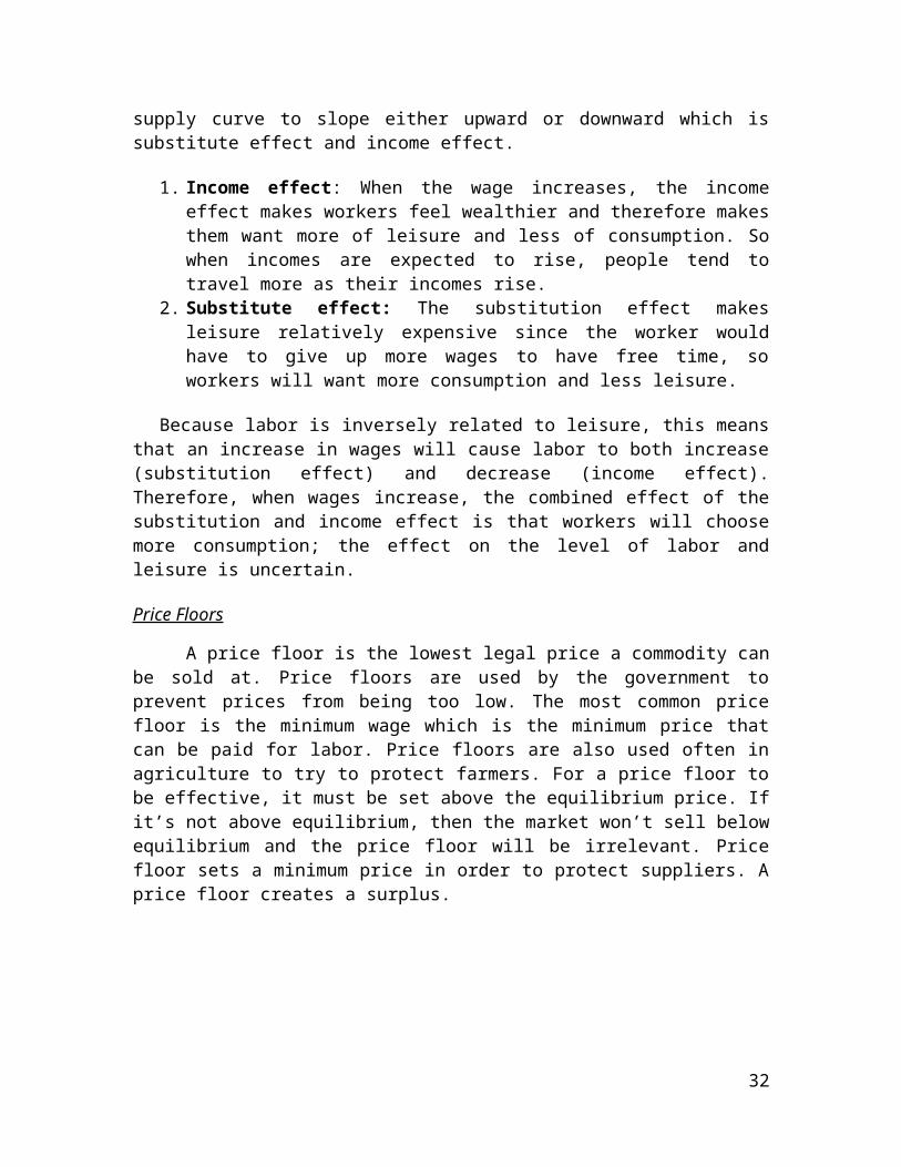
Figure 3.1: A Shift in Labor Supply

Based on the Figure 3.1, it shows that the minimum wages of Americans have risen too high to $15 an hour in some cities such as Seattle, San Francisco and Los Angeles. The minimum wages has increase from $10 to $15, thus affecting the supply of labor to decrease. This tends to reduce the employment rate, thus hurting young and less-educated workers the most. Therefore, when labor supply decrease from S1 to S2, the equilibrium wage rises from $10 to $15. At this higher wage, companies hire less labor, so employment falls from 150 laborsto 100 labors.As a result of a minimum wage,companiesgenerally experience dramatic increases in the wage expenses as they rely to a large extent on unskilled labor, since a minimum wage eliminates the ability ofcompanies to haggle wages for their lowest-level employees. The article states that according to the U.S. Department of Labor, the minimum wage increased about fifty percent between 2009 and 2014, going from $10 to $15 per hour. With this dramatic increase in minimum wages, it will affect the local employment for companies’ feel that the minimum wage is a large expense for an unskilled worker, which can cause them to imposestricter decision criteria for hiring or reduce on hiring altogether.For cities like Seattle, with a relatively more educated workforce and dynamic labor market, it is worth taking the risk while for cities such as L.A and Washington D.C, with their large populations of less-educated workers, including unskilled immigrants, such increase is extremely risky.

25

I1

I2

Consumption

Hours of Leisure

I3

$1500

$900

060 100

Wages Affect Labor Supply

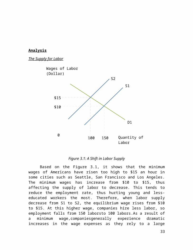
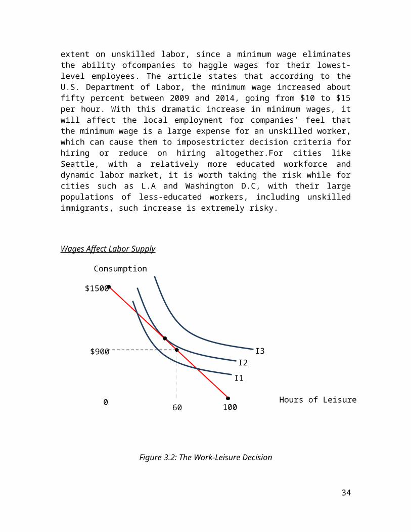
Figure 3.2: The Work-Leisure Decision

Workers try and maximize their utility based on their preferences between having free time and having money, and on their budget constraint.A worker's budget constraint can pivot with a change in the wage. According to the Figure 3.2, if the wage increases, the curve pivots outwards (I3). If the wage drops, then the curve pivots inwards (I1). Therefore, assuming worker are awake for 100 hours per week with the minimum wage of $15, for every hour a worker works, he earns $15, which he spend on consumption goods. Thus, his wage $15 reflects the trade-off the worker faces between leisure and consumption. For every hours of leisure he gives up, he works one more hour and gets $15 of consumption. This graph shows a worker’s budget constraint.If he spends all 100 hours enjoying leisure, he has no consumption butif he spends all 100 hours working, he earns a weekly consumption of $1,500 but no time for leisure. If he works a normal 40 hours week, he enjoys 60 hours of leisure and has weekly consumption of $900.

26

I1I2

Consumption

Hours of Leisure0 60 10070

$15

Labor Supply

Wages of Labor (Dollar)

Hours of LeisureSupplied

$10

100 1500

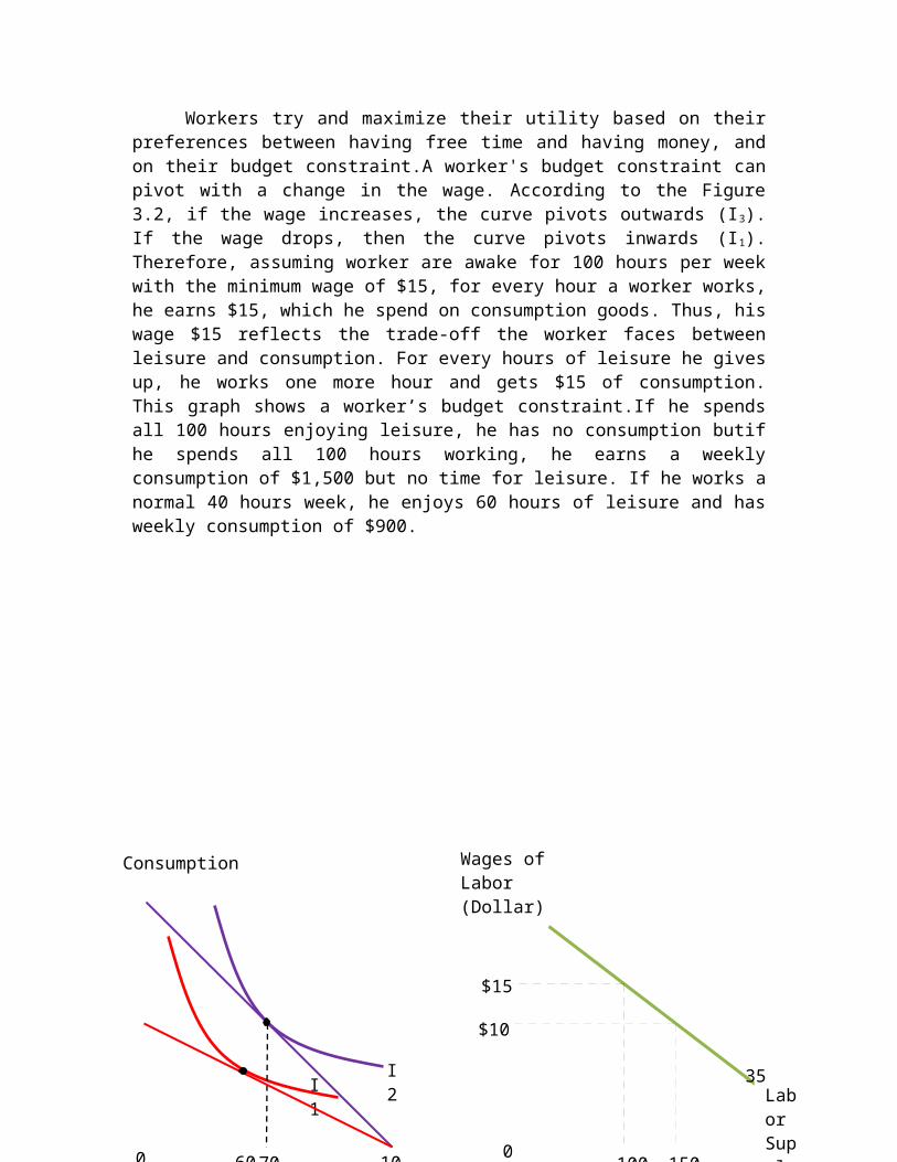
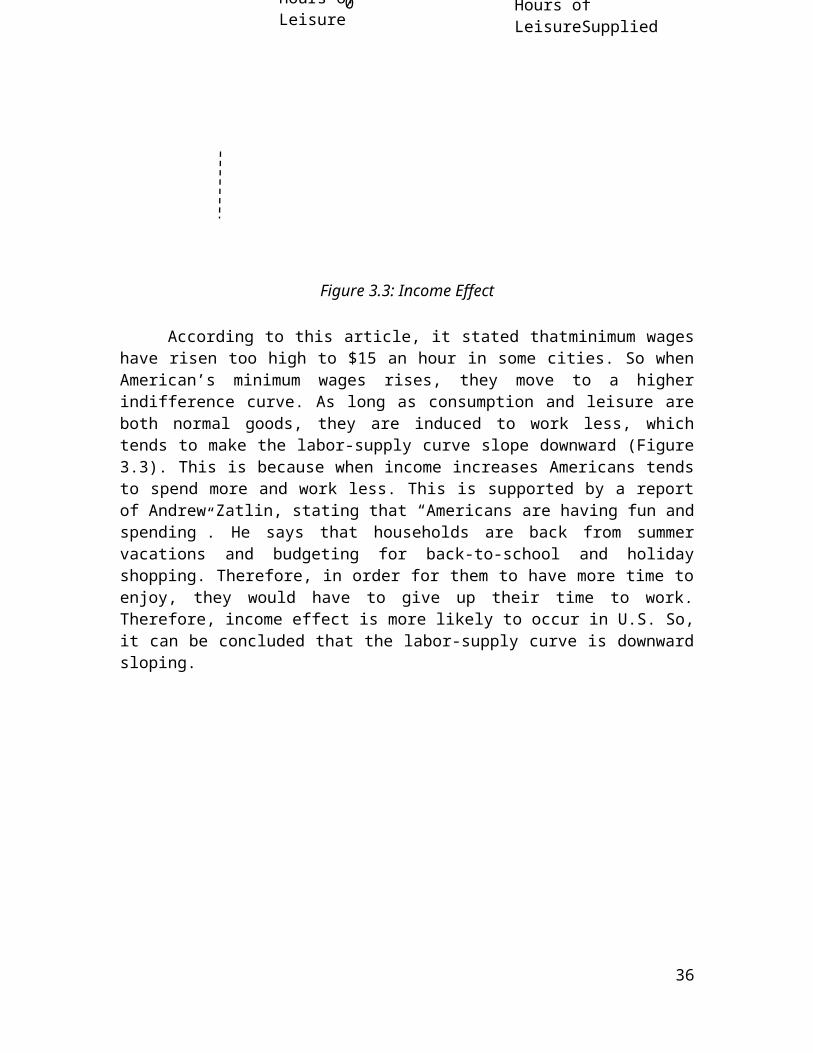
Figure 3.3: Income Effect

According to this article, it stated thatminimum wages have risen too high to $15 an hour in some cities. So when American’s minimum wages rises, they move to a higher indifference curve. As long as consumption and leisure are both normal goods, they are induced to work less, which tends to make the labor-supply curve slope downward (Figure 3.3). This is because when income increases Americans tends to spend more and work less. This is supported by a report of Andrew Zatlin, stating that “Americans are having fun and spending”. He says that households are back from summer vacations and budgeting for back-to-school and holiday shopping. Therefore, in order for them to have more time to enjoy, they would have to give up their time to work. Therefore, income effect is more likely to occur in U.S. So, it can be concluded that the labor-supply curve is downward sloping.

27

Minimum Wages

Wages Rate

Quantity of Labor

Labor Supply

Labor Demand

$10

150

$15

100 200

Unemployment

0

Equilibrium

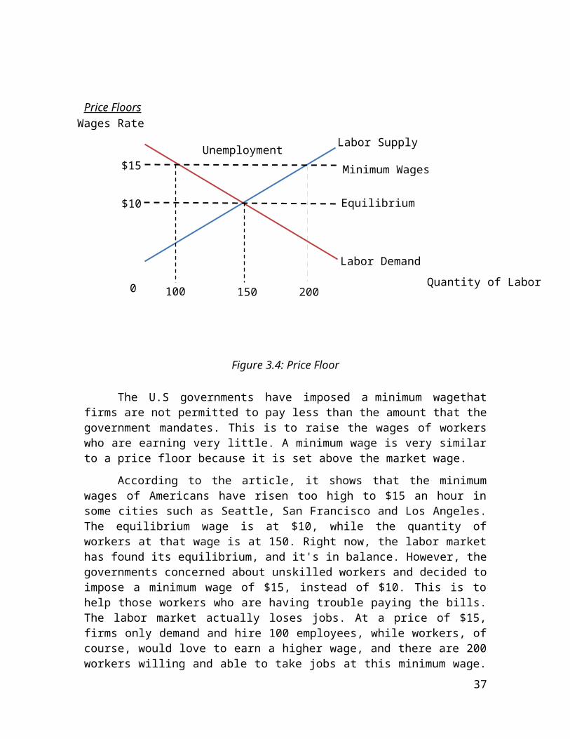
Price Floors

Figure 3.4: Price Floor

The U.S governments have imposed a minimum wagethat firms are not permitted to pay less than the amount that the government mandates. This is to raise the wages of workers who are earning very little. A minimum wage is very similar to a price floor because it is set above the market wage.

According to the article, it shows that the minimum wages of Americans have risen too high to $15 an hour in some cities such as Seattle, San Francisco and Los Angeles. The equilibrium wage is at $10, while the quantity of workers at that wage is at 150. Right now, the labor market has found its equilibrium, and it's in balance. However, the governments concerned about unskilled workers and decided to impose a minimum wage of $15, instead of $10. This is to help those workers who are having trouble paying the bills. The labor market actually loses jobs. At a price of $15, firms only demand and hire 100 employees, while workers, of course, would love to earn a higher wage, and there are 200 workers willing and able to take jobs at this minimum wage. So, the quantity of labor demanded falls, while the quantity of labor supplied rises. Since, there are 200 workers looking for jobs, but the firms only hire 100, that mean there is a surplus of 100 workers. The surplus is unemployment. A minimum wage set above the market wage will increase unemployment by 100 workers.

Conclusion

In conclusion, when minimum wages of Americans increase, the supply of labor will decrease.Besides, the increase in minimum wagescauses labor to decrease (income effect). Moreover, increase in minimum wages will cause unemployment because the quantity of labor demanded decrease, while the quantity of labor supplied increase.

28

29

Summary

Central Illinois farmer, Rodney Weinzier knew that it is in reality a mere matter of supply and demand that the corn costs have fallen as yields have increased. In the last ten years, with the exception of a drought year in 2012, advances in seed technology, plant food, equipment and planting methods have contributed to historic corn yields. On the surface, an increase in production would typically be seen as a positive, but the lack of a market for corn has led to corn being sold at dollars off the profit margin per bushel. Thus, low prices of the corn per bushel have created more stress for the average farmer. Although there has been a recent rise in prices to $4.20 per bushel, that price still isn't enough as there is a study by the University of Illinois shows that $4.30 is the break-even price for a farmer.

Discussion

Demand and Supply

Supply and demand are perhaps one of the most fundamental concepts of economics and they are the backbone of a market economy. Demand refers to how much (quantity) of a product or service is desired by buyers. The quantity demanded is the amount of a product people are willing and able to buy at a certain price; the relationship between price and quantity demanded is known as the demand relationship. Supply represents how much the market can offer. The quantity supplied refers to the amount of a certain good producers are willing and able to supply when receiving a certain price. The correlation between price and how much of a good or service is supplied to the market is known as the supply relationship. Price, therefore, is a reflection of supply and demand.

The relationship between demand and supply underlie the forces behind the allocation of resources. In market economy theories, demand and supply theory will allocate resources in the most efficient way possible.

The Law of Demand

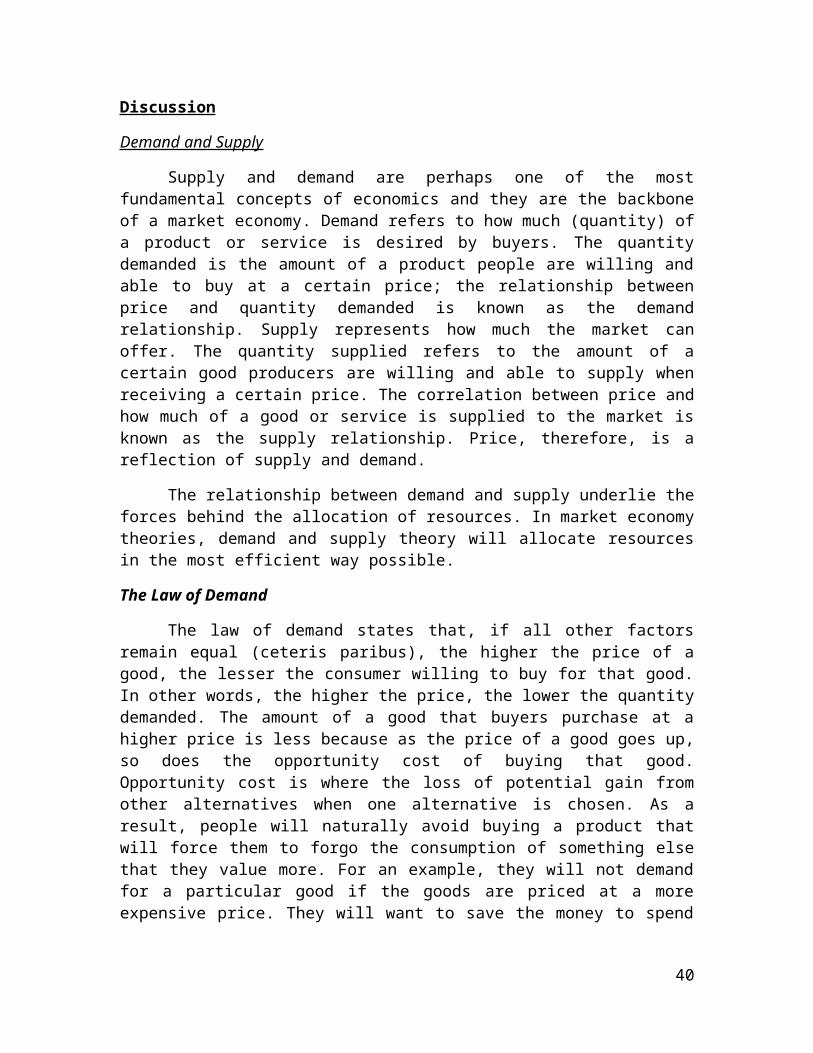
The law of demand states that, if all other factors remain equal (ceteris paribus), the higher the price of a good, the lesser the consumer willing to buy for that good. In other words, the higher the price, the lower the quantity demanded. The amount of a good that buyers purchase at a higher price is less because as the price of a good goes up, so does the opportunity cost of buying that good. Opportunity cost is where the loss of potential gain from other alternatives when one alternative is chosen. As a result, people will naturally avoid buying a product that will force them to forgo the consumption of something else that they value more. For an example, they will not demand for a particular good if the goods are priced at a more expensive price. They will want to save the money to spend on other goods and services. The graph below shows that the curve is a downward slope.

30

Q0DD

Q

P

Q10

P0

P1

A

B

P1

P0

SSP

Q0 Q0 Q1

C

D

AandB are points on the demand curve. Each point on the curve reflects a direct correlation between quantity (Q) and price (P). The demand relationship curve illustrates the negative relationship between price and quantity. The higher the price of a good, the lower the quantity demanded and the lower the price, the higher the quantity demanded.

The Law of Supply

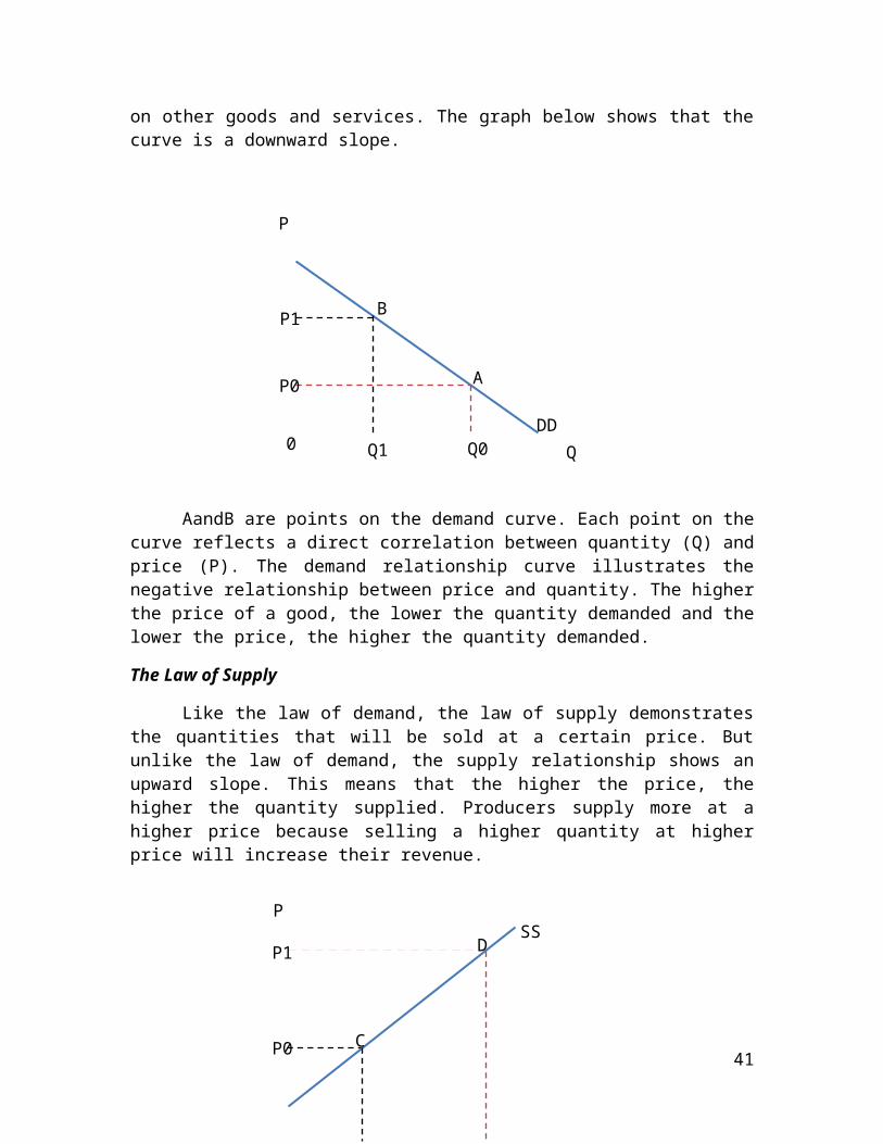
Like the law of demand, the law of supply demonstrates the quantities that will be sold at a certain price. But unlike the law of demand, the supply relationship shows an upward slope. This means that the higher the price, the higher the quantity supplied. Producers supply more at a higher price because selling a higher quantity at higher price will increase their revenue.

C and D are points on the supply curve. Each point on the curve reflects a direct correlation between quantity (Q) and price (P). The supply relationship curve illustrates the positive relationship between price and quantity. The higher the price of a good, the higher the quantity supplied and the lower the price, the lower the quantity supplied.

31

P

Q

SS

DD

Pe

Qe

Equilibrium

0

P

Q

SS

DD

Pe

Qe

P1

Qd Qs

SurplusQs >Qd

0

Equilibrium

When supply and demand is equal which is when the supply function and demand curve intersect, the economy is said to be at equilibrium. At this point, the allocation of goods is at its most efficient because the amount of goods being supplied is exactly the same as the amount of goods being demanded. Thus, the buyer and seller are satisfied with the current economic condition. At the given price, suppliers are selling all the goods that they have produced and consumers are getting all the goods that they are demanding.

Based on the graph above shown that equilibrium occurs at the intersection of the demand and supply curve, which indicates no allocative inefficiency. At this point, the price of the goods will be Pe and the quantity will be Qe. These figures are referred to as equilibrium price and equilibrium quantity. However, in the real market place equilibrium can only ever be reached in theory, so the prices of goods and services are constantly changing in relation to fluctuations in demand and supply.

Disequilibrium

Disequilibrium occurs whenever the price or quantity is not equal to the equilibrium price and equilibrium quantity.

1. Excess Supply (Surplus)

32

P

Q

SS

DD

Pe

Qe

P2

Qd Qs

Shortage

Qd> Qs

0

At the beginning, the equilibrium price is Pe and equilibrium quantity is Qe. When the price of that good increase, the suppliers are trying to produce more goods, which they hope to sell to increase profits, but those consuming the goods will find the product less attractive and purchase less because the price is too high.This has increased the price from Pe to P1, which has led the quantity demanded less than the quantity supplied. This has caused the disequilibrium of market economy, surplus. Therefore, if the price is set too high, excess supply will be created within the economy and there will be allocative inefficiency.

2. Excess Demand (Shortage)

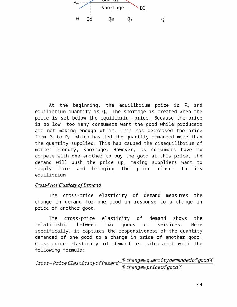
At the beginning, the equilibrium price is Pe and equilibrium quantity is Qe. The shortage is created when the price is set below the equilibrium price. Because the price is so low, too many consumers want the good while producers are not making enough of it. This has decreased the price from Pe to P2, which has led the quantity demanded more than the quantity supplied. This has caused the disequilibrium of market economy, shortage. However, as consumers have to compete with one another to buy the good at this price, the demand will push the price up, making suppliers want to supply more and bringing the price closer to its equilibrium.

Cross-Price Elasticity of Demand

The cross-price elasticity of demand measures the change in demand for one good in response to a change in price of another good.

The cross-price elasticity of demand shows the relationship between two goods or services. More specifically, it captures the responsiveness of the quantity demanded of one good to a change in price of another good. Cross-price elasticity of demand is calculated with the following formula:

Cross−Price Elasticity of Demand=%change∈quantity demanded of good X%change∈price of good Y

The cross-price elasticity may be a positive or negative value, depending on whether the goods are complements or substitutes. If two products are complements, an increase in demand for one is accompanied by an increase in the quantity demanded of

33

A

Quantity of Good B

Quantity of Good A

0

B

C

D

the other. For example, an increase in demand for cars will lead to an increase in demand for fuel. If the price of the complement falls, the quantity demanded of the other good will increase. The value of the cross-price elasticity for complementary goods will thus be negative.

A positive cross-price elasticity value indicates that the two goods are substitutes. For substitute goods, as the price of one good rises, the demand for the substitute good increases. For example, if the price of coffee increases, consumers may purchase less coffee and buy more tea. Conversely, the demand for a substitute good falls when the price of another good is decreased. In the case of perfect substitutes, the cross elasticity of demand will be equal to positive.

Production Possibilities Frontier (PPF)

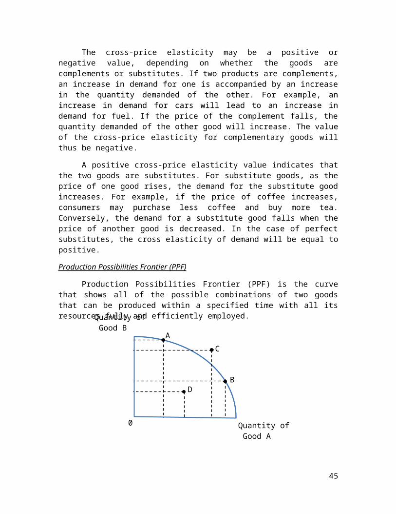
Production Possibilities Frontier (PPF) is the curve that shows all of the possible combinations of two goods that can be produced within a specified time with all its resources fully and efficiently employed.

The economy can produce at any combination on or inside the curve (A, B, D). Point C outside the curve is not attainable.

There are four assumptions on PPF, which are full employment and productive efficiency, producing two goods, fixed resources and fixed technology. It is said that points A and B are attainable and efficient because all resources are fully and efficiently employed. Points inside the curve (D) is attainable and inefficient because resources are not fully and efficiently employed. Point outside the curve (C) is unattainable because of limited resources.

Shifts in the Economy’s Production Possibilities Frontier

34

A

Capital Goods

Consumer Goods

A’

F0

This is when there is an increase in available resources or technological advance that benefits consumer goods.

Analysis

35

Q0 Q1

$4.30

$4.20

Quantity of Corn

Price of Corn S1

S2

0

$4.30$4.20

Q1 Q2

Price of Corn

DD

Quantity of Corn Cereal0

Demand and Supply

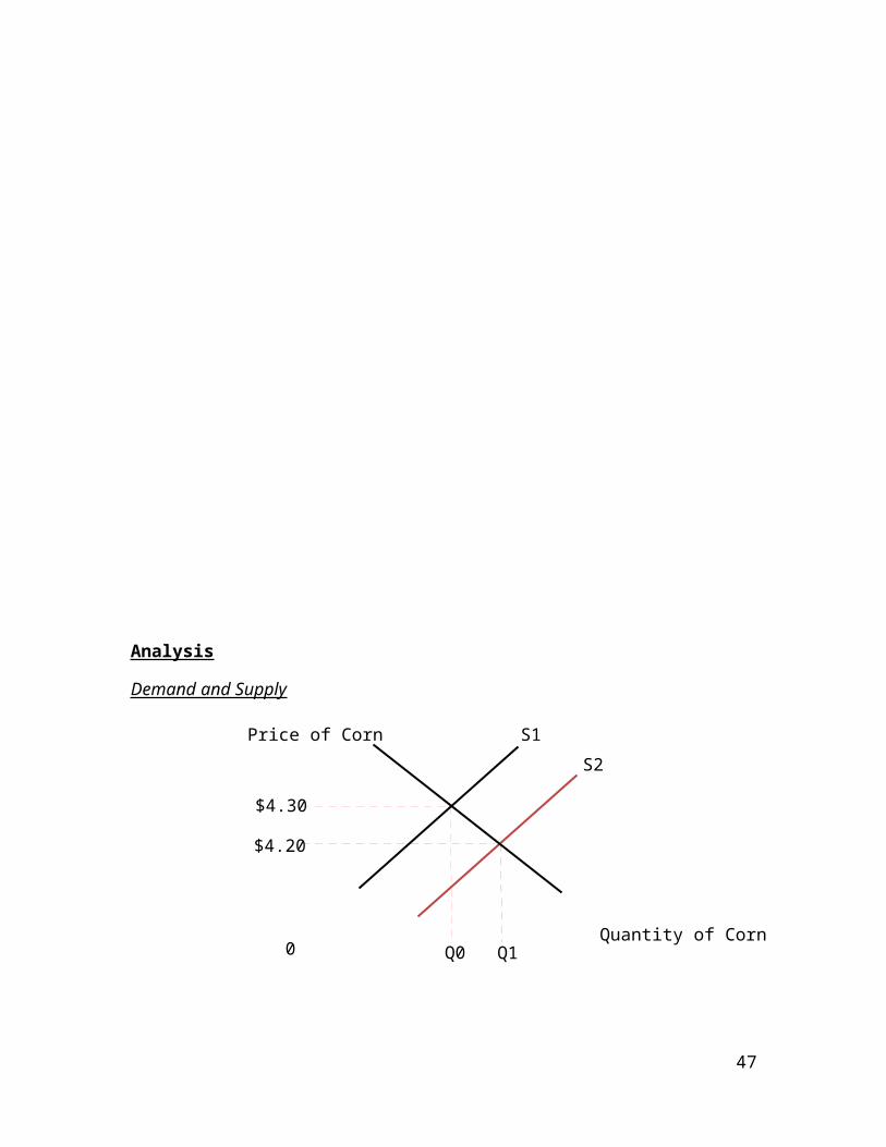
Figure 4.1: Shift in the Supply Curve of Corn

Based on the Figure 4.1, the price equilibrium is $4.30 and the quantity equilibrium is Qo. The advancement in seed technology, fertilizer, equipment and planting methods for corn has increase the production of corn. Thus, it will shift in the supply curve of corn from S1 to S2 due to the improvement of technology. This has decrease the price of corn to $4.20, and increase the quantity supplied to Q1, which is more than the equilibrium quantity, Q0. Disequilibrium of market condition has occurred, which is surplus. The market condition where the suppliers produce more goods than what the consumer need that the quantity supplied (Q1) is more than the quantity demanded (Q0). This is because when the price of corn has reduced, the consumers are now more willing and able to purchase more corn as according to the law of demand.

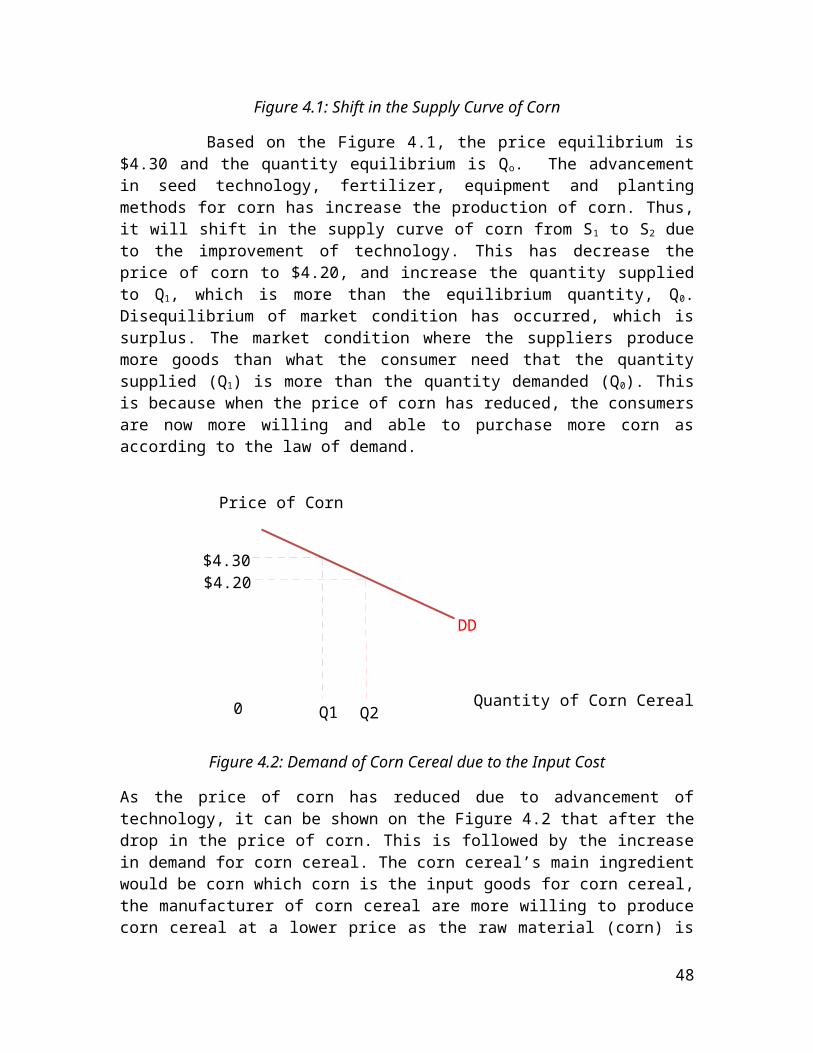
Figure 4.2: Demand of Corn Cereal due to the Input Cost

As the price of corn has reduced due to advancement of technology, it can be shown on the Figure 4.2 that after the drop in the price of corn. This is followed by the increase in demand for corn cereal. The corn cereal’s main ingredient would be corn which corn is

36

A

Quantity of Corn

Quantity of Wheat0

B

C

D

the input goods for corn cereal, the manufacturer of corn cereal are more willing to produce corn cereal at a lower price as the raw material (corn) is now cheaper. Thus, the demand for corn cereal will therefore largely increase. In this situation, it can only be good news for the manufacturer of corn cereal as the cost of production has largely reduced. They are able to produce vast amount of corn cereal with a much lower cost.

Cross-Price Elasticity of Demand

The cross-price elasticity of demand is a positive or negative number depends on whether the two goods are substitutes or complements. We assume that corn and wheat are substitute goods. Substitutes are goods that typically used in place of one another. A decreases in corn price will induces the producer to manufacture products by using corn. The producer will switch the input goods from wheat to corn due to the drop in corn price. Thus, the price of corn and the quantity of wheat demanded move in the same direction, the cross-price elasticity is positive.

Besides, the corn and farm equipment are complement goods, which means goods that are typically used together. The advancement of technology has decrease in the price of corn. Therefore, farmers will plant and harvest more of this commodity and will need more farm equipment to harvest the crops.  In this case, the cross-price elasticity is negative, indicating that the drop in price of corn will increase the quantity of farm equipment demanded.

Production Possibilities Frontier (PPF)

This is a production possibilities frontier graph that makes the assumption that the economy only produces two goods, wheat and corn. It has also assumed that it has already in a condition where it has full employment and productive efficiency, the technology is fixed and the resources available are also fixed.

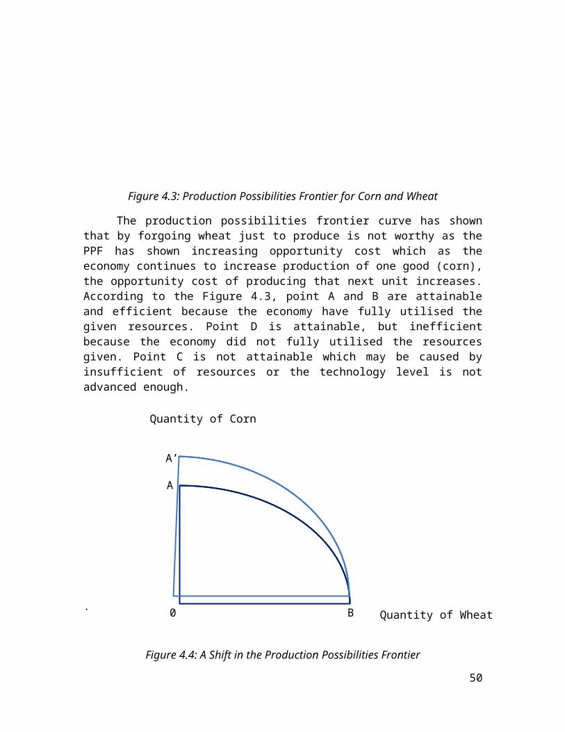
Figure 4.3: Production Possibilities Frontier for Corn and Wheat

The production possibilities frontier curve has shown that by forgoing wheat just to produce is not worthy as the PPF has shown increasing opportunity cost which as the economy continues to increase production of one good (corn), the opportunity cost of

37

A

Quantity of Wheat

Quantity of Corn

A’

B0

producing that next unit increases. According to the Figure 4.3, point A and B are attainable and efficient because the economy have fully utilised the given resources. Point D is attainable, but inefficient because the economy did not fully utilised the resources given. Point C is not attainable which may be caused by insufficient of resources or the technology level is not advanced enough.

.

Figure 4.4: A Shift in the Production Possibilities Frontier

As the article mentioned, advances in seed technology, fertilizer, equipment and planting methods have led to historic corn yields. This is a good example of demonstrating how advance in seed technology can further increase the production of crops. Based on the Figure 4.4, with the advancement in seed technology, the economy can now move the PPF curve outward from A to A’ by making the choice of producing corn only.

Conclusion

To conclude that when the supply of corn has increased due to the advance in technology, the price of corn has decreased. The relationship between corn and corn cereal is complements, which means that when the price of corn decreases, the quantity demanded for corn cereal will subsequently increase. The cross-price elasticity of demand for corn and wheat is positive, because they are substitute goods and the quantity demanded for wheat decrease when a decrease in corn price. Moreover, farm equipment and corn are complement goods, therefore the cross-price elasticity is negative and the quantity of farm equipment demanded increases as the price of corn decreases. Furthermore, with the advances in seed technology, fertilizer, equipment and planting methods, farmers should use it to fully produce corn instead of wheat.

38

39

Summary

The creator, Mark Pivac who is an Australian engineer has built a robot that can build houses in two days, and could work every day to build houses for people. The robot

40

is called as Hadrian, it was a solution to the lack of available workers for bricklaying as the average age of the industry is getting much higher, and the robot might be able to fill some of that gap. However, there is also some people are arguing that it will take the jobs of human bricklayers and this causes unemployment in bricklaying field in Australia. This is because human house-builders have to work for four to six weeks to put a house together, and have to take weekends and holidays. The robot can work much more quickly and doesn’t need to take breaks. In fact, Hadrian works by laying 1000 bricks an hour, letting it put up 150 houses a year. Also, Mark Pivac will now work to commercialise the robot, first in West Australia but eventually globally.

Discussion

Demand for Labor

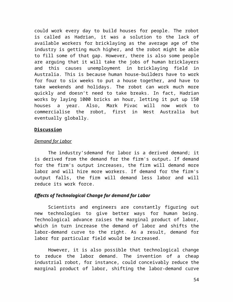
The industry’sdemand for labor is a derived demand; it is derived from the demand for the firm's output. If demand for the firm's output increases, the firm will demand more labor and will hire more workers. If demand for the firm's output falls, the firm will demand less labor and will reduce its work force.

Effects of Technological Change for demand for Labor

Scientists and engineers are constantly figuring out new technologies to give better ways for human being. Technological advance raises the marginal product of labor, which in turn increase the demand of labor and shifts the labor-demand curve to the right. As a result, demand for labor for particular field would be increased.

However, it is also possible that technological change to reduce the labor demand. The invention of a cheap industrial robot, for instance, could conceivably reduce the marginal product of labor, shifting the labor-demand curve to the left, reducing the demand for labor. Economists call this labor-saving technological change. This is because the invention of the robot has become the substitute for human labor, the industry would prefer robot rather than human as it is more effective.

History suggests, however, that most technological progress is instead labor- augmenting. Think about secretaries that used to type letters on typewriters long time ago. It may be now replace typewriter with modern computers that can easily duplicate and edit documents, one secretary now can do the same amount of work as four secretaries could in the days of typewriters. That means the labour of the secretary has been augmented by the advance of technology, one secretary is now worth four secretaries in the past. When a technology is improving then it means the population and labour force grows, and actually grow the number of ‘effective workers’ faster than the population grows.

Diminishing marginal product

41

Quantity of Output

300280240

180

100

Quantity of Output worker 1 2 3 4 50

MP, Value of MP

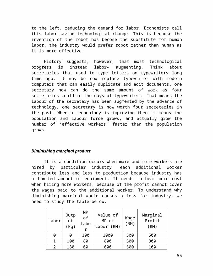
It is a condition occurs when more and more workers are hired by particular industry, each additional worker contribute less and less to production because industry has a limited amount of equipment. It needs to bear more cost when hiring more workers, because of the profit cannot cover the wages paid to the additional worker. To understand why diminishing marginal would causes a loss for industry, we need to study the table below.

LaborOutput

(kg)MP of Labor

Value of MP of Labor (RM)

Wage (RM)

Marginal Profit (RM)

0 0 100 1000 500 5001 100 80 800 500 3002 180 60 600 500 1003 240 40 400 500 -1004 280 20 200 500 -3005 300

Based on the table above, when number of worker increases, the quantity of output will increase. At the same time, diminishing marginal product occurs, when the number of labor increases, the marginal product (MP) declines.

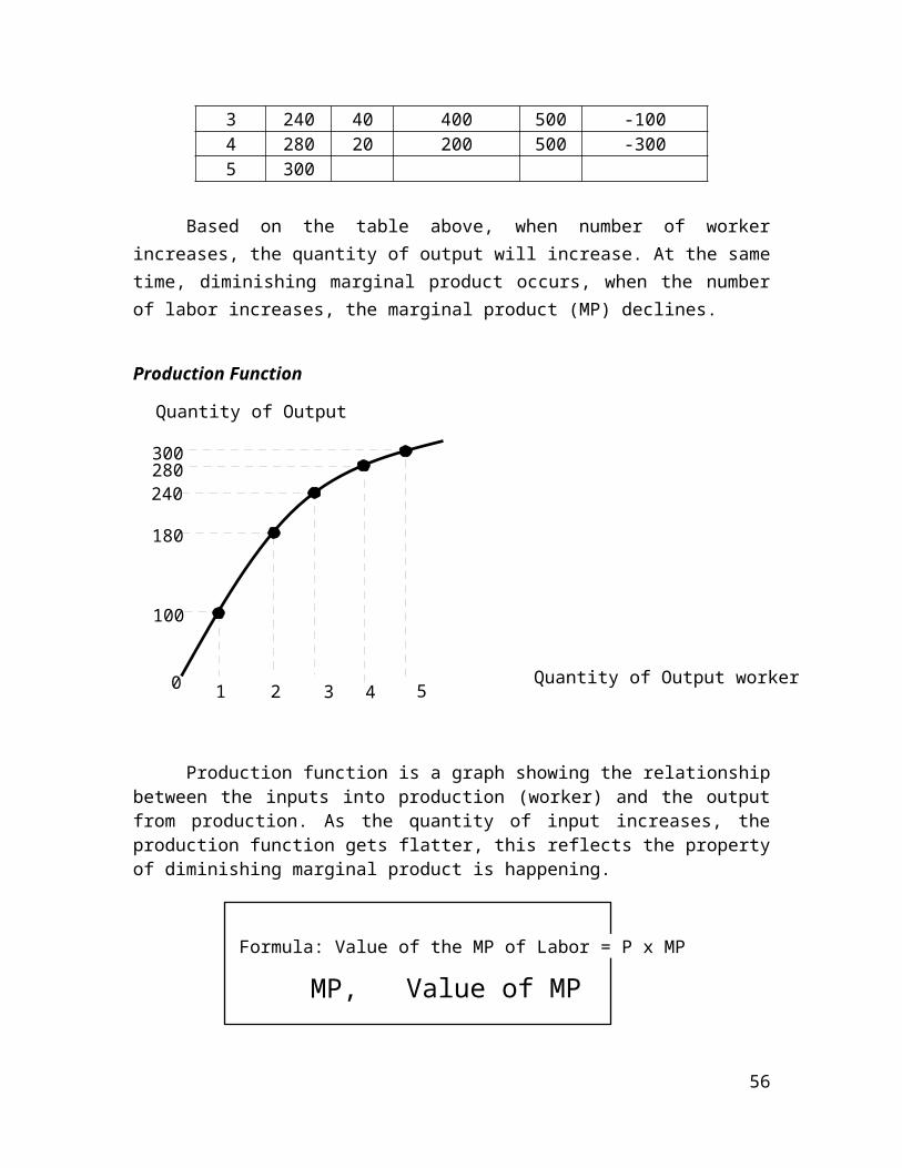
Production Function

Production function is a graph showing the relationship between the inputs into production (worker) and the output from production. As the quantity of input increases, the production function gets flatter, this reflects the property of diminishing marginal product is happening.

42

Formula: Value of the MP of Labor = P x MP

A decrease in marginal product of labor (MPL) will cause a reduction for value of the MP. To calculate the marginal profit, we need to minus worker’s contribution to the value of MP from the wages that pay to worker. Let’s assume that a kilogram of the output is RM10, if an additional worker produces 80 kg of output, the worker has produced RM800 of revenue, so the first worker has helped the firm to earn a profit of RM 500, because the value of MP is more than wage. However, the third worker causes the firm to have a loss of -RM100 because value of MP is less than wage. Since the primary goal of an industry is to maximize the profit, it force to stop hiring additional worker in this field.

Analysis

Demand for Labor

In general, when there is high demand of the output, the demand for labor will increase, this is because demand of labor is derived demand. In this case, the demand for

43

brick house in Australia is high, and the demand of labor is supposed to increase. According to Master Builders Association of NSW executive director Brian Seidler, the labor drought came amid increased demand for bricklayers not just in the new home market but from thousands of renovators. “Nearly 65 per cent of existing housing stock is 25-35 years old. They all need renovations. The problem is we’ve got to get people interested in the industry,” MrSeidler said. However, in this case, the demand for labor has decreased, this is due to the invention of Hadrian, a robot which become the substitute to the available bricklayer. The shortage of bricklayer has been solved, and demand for bricklayer is no longer higher.

Figure 5.1: Demand for Labor

The invention of robot, Hadrian has assisted Australia to solve the shortage of available labor. However, this technology has led to labor-saving technological change also. The demand of labor is decreasing in Australia, thus shifting the demand for labor curve from D0 to D1 that has shown in Figure 5.1. This is because Hadrian has become the substitute to the labor. The invention of Hadrian allows more brick houses to be built in short period, whereas labor need a long period to build more brick houses. Human house builders have to work for four to six weeks to put a house together, and have to take weekends and holidays. The robot can work much more quickly and does not need to take breaks. Although Hadrian has benefits the demand market for brick house, there is also some disadvantages. Since the demand labor has reduced, the wages of the labor will be affected. Wages will be reduced, industry has more options regarding the type of inputs to build the brick houses, either Hadrian or human labor. There is a high possibility that the unemployment rate will rise in Australia. Bricklayers will lose their job, and they have to look for other highly demanded job.

44

Value of the Marginal Product

Quantity of Bricklayer

Value of Marginal Product

Profit- maximizingquantity

MarketWages

0

Figure 5.2: The Value of the Marginal Product of Labor

There are few factors that affect industry would not hire more workers. The invention of Hadrian is one of the factors that results in industry has no interest in hiring more workers. Another factor is that the value of the marginal product of labor. According to the Figure 5.2, when the marginal product of labor is more than market wages, the industry will hire worker. Similarly, when the marginal product of labor is less than market wages, the industry will not hire additional workers. The reason is industry will make a loss, the revenue earned by the bricklayers is not adequate to cover the wages rate. All these are because of property of diminishing marginal product. If the industry hire more workers, each contribution by the workers will be reduced, because of limited equipment. The marginal product will decrease gradually, and this will also lead to a drop for the value of marginal product. The industry would not hire workers when the contribution made by the workers cannot cover the wages paid to workers. The industry will maximize the number of worker until the wages rate equal to marginal product of labor. The intersection of the marginal product of labor curve with the market wage determines the number of workers that the industry hires.

Conclusion

Initially, the high demand for brick houses in Australia and shortage of bricklayer have led to a rise in demand of bricklayer. However, Mark Pivac, the Australian Engineer had invent a robot, Hadrian to substitute the job for bricklayer. As a result, shortage of bricklayer has solved, the demand of bricklayer is decreasing and automatically the market wages rate will be reduced. There is a high possibility that the unemployment rate in Australia arise due to the low demand for bricklayer, they need to find other highly-demanded job. The decrease in demand labor not just because of the substitute of robot, Hadrian, but also because of property of diminishing marginal product. The industry will only maximize the number of worker until the marginal revenue product of labor meet the market wage ratein order to achieve its primarily goal which is to maximize profit.

45

46

Summary

This article talks about a new product that KFC introduced for its customers in conjunction with the festive season. The product is called the ‘KFC Ayam Kicap Meletup’. With the tagline “So Meletup Sure Must Share”, it features a combination of Malaysia’s favorite condiments and unique soy sauce that suits local taste buds. The KFC Ayam Kicap Meletup’s price ranges from RM 10.95 to RM 74.25 with various side dishes and free cutlery sets. It is available at all KFC restaurants nationwide.

Discussion

Utility

Utility is an abstract measure of the satisfaction or happiness that a consumer receives from a bundle of goods. According to economists, if a bundle of goods provides more utility than the other, it is to be preferred by consumers. By using an indifference curve, we are able to find out how consumers maximize utility with the choices they make. There are four properties of indifference curves:

1) Higher indifference curves are preferred to lower ones. People usually prefer to consume more goods rather than less.

2) Indifference curves are downward slopping. The slope reflects the rate at which the consumer is willing to substitute one good for the other. If one good is reduced, the quantity of the other good must increase for the consumer to be equally happy. This also assumes that the marginal rate of substitution is always positive.

3) Indifference curves do not cross. It is because at the point of intersection, the higher curve will give as much utility as of the two goods as is given by the lower indifference curve. This is absurd and impossible.

4) Indifferent curves are bowed inwards. The slope of an indifference curve is the marginal rate of substitution- the rate at which the consumer is willing to trade off one good for the other. It reflects the consumer’s greater willingness to give up one good that he already has in large quantity. People are more willing to trade away goods they have in abundance and less willing to trade away goods they have little, thus it is bowed inwards.

A budget constraint illustrates the limit on the consumption bundles that a consumer can afford. By combining the budget constraint with indifferent curve, we are able to see how consumers maximize their utility within their income. The point where the budget constraint touches the indifference curves is the optimum point. It represents the best combination of bundled goods available to the consumer. At the optimum, the slope of the indifference curve equals the slope of the budget constraint. Thus, the consumer chooses consumption of the two goods so that the marginal rate of substitution equals the relative price.

47

Market structure

Monopolistic competition is a market structure in which many firms sell products that are similar but not identical. It has the following attributes:

1) Many SellersThere are many firms competing for the same group of customers.

2) Product DifferentiationEach firm produces a product that is slightly different from those of other firms.

3) Price MakerThey can easily change the price strategy of the market. If one company changes their product price, it will also influence the other firms to change their prices.

4) Free Entry and ExitFirms can enter and exit the market without restriction. The number of firms in the market adjusts until economic profits are driven until zero.

Economies and Diseconomies of Scale

Economies of scale is the property whereby long-run average total cost falls as the quantity of output increases. Diseconomies of scale is the property whereby long-run average cost rises as the quantity of output increases. Constant returns to scale is the property whereby long-run average total cost stays the same as the quantity of output changes. Economies of scale often arise because higher production levels allow specialization among workers. Diseconomies of scale can arise because of coordination problems that are inherent in any large organization.

At low levels of production, the firm benefits from increased size because it can take advantage of greater specialization. By contrast, the benefits of specialization have been realized at high levels of production, and coordination problems become more severe as the firm grows larger. Thus, long-run average cost falls at low levels of production because of increasing specialization. It rises at high levels of production because of increasing coordination problems.

48

0

0

MU

Quantity of KFC

TU

Quantity of KFC

Point A

Analysis

Utility

Based on the article, KFC introduced a new product, which is the KFC AyamKicapMeletup. This is because they need to attract consumers and increase the marginal utility of customers. Assuming that the KFC Original Flavored Fried Chicken was KFC’s best-selling product before the new product is introduced. In the earlier stages of introducing KFC Original Flavored Fried Chicken, consumers tend to buy the KFC Original Flavored Fried Chicken and their total satisfaction increases accordingly. However, as the total satisfaction of customers increases day by day, the marginal utility towards KFC decreases with each additional unit of the same good consumed. Based on Figure 6.1, when the total utility of the consumer reaches the maximum point (Point A), the marginal utility of consumer will become zero. Therefore, the additional satisfaction of consumer toward KFC will decline and this makes the marginal curve downward-slopping. This downward-sloping marginal utility curve has a significant effect for consumer behavior regarding demand of KFC. Hence, KFC introduces a new product to increase the satisfaction of consumers.

Figure 6.1: Relationship between Total Utility and Marginal Utility

49

0

B0

A0

200

Indifference Curve

Quantity of KFC AyamKicapMeletup (Units)120000

100000

5000

Quantity of KFC Original Flavored Fried Chicken (Units)

Figure 6.2: Indifference Curve

Based on the article, the KFC AyamKicapMeletup is expected to shift the consumer’s preferences towards this new product. The indifference curve in Figure 6.2 shows the combinations of KFC Original Flavored Fried Chicken and KFC AyamKicapMeletup with which the consumer is equally satisfied. The points A and B are on the same curve. Thus, consumers are indifferent among both combinations.

With the new product, consumers will increase their consumption of the KFC AyamKicapMeletup. From the Figure 6.2, we can see that the quantity of the KFC Red Hot decrease from 1000 units to 500 units while the quantity of AyamKicapMeletup increase from 20 units to 1200 units. This is because KFC AyamKicapMeletup is the new product that is introduced by KFC and consumers are curious of it, thus consumers will buy more KFC AyamKicapMeletup. This in return increases the satisfaction level of consumer towards KFC product. When consumer buy each unit of KFC AyamKicapMeletup, they will give up more and more KFC Original Flavored Fried Chicken. The consumer’s preference shifts from point A to point B (Figure 6.2). This also explains why the indifferent curve is bowed inward.

50

0

Price of KFC

D1 S1

S1

S1

S1

S1

S1

S1

Quantity of KFC

0

Price of KFC

S1

S1

Quantity of KFC

Market Structure

KFC is a monopolistic competition firm. KFC sell products that are different from each other but there are no perfect substitutes for their products in terms of quality, branding and location. KFC also sell differentiate product such as KFC Red Hot Chicken and KFC Original Flavored. There are many firms in the market due to the unrestricted freedom for other firms to enter to industry. It mean that firms can easily entry and exit the market. When the market make a profit, many firm will entry into the market without any restriction whereas when the market make a loss, the firm will exit the market. Due to this condition, KFC will make zero economic profit in long run. We can analyze from the Figure 6.3.

Figure 6.3: KFC Makes AZero Economics Profit in the Long Run

Based on the Figure 6.3, we can assume that the demand of KFC increase and cause the price of KFC increase from P1 to P2. Hence, KFC are making profits and this situation have cause new firm to enter the market. The entry increases the number of sellers and numbers of KFC products. When the number of sellers increase, supply curve increase from S1 to S2, it causes the price of KFC decrease from P2 to P1. When the price decrease to the original price P1, KFC does not make any profit and KFC is in the market have an incentive to exit. Therefore, the remaining firm earn exactly zero economic profit in the long run.

Besides, KFC cannot limit their production as they have many competitors in the fast food chain such as MC Donald and Burger King. For the pricing strategies, KFC ignored the price of the competitors and set up their own price. This can explain why KFC is a price maker. As a monopolistic competition market, KFC set their own price based on the cost and there’s no perfect substitute for the tastiness of their meals. The price of the AyamKicapMeletup ranges from RM10.95 to RM74.25 with different quantities and side dishes.

51

01 Q21Q11

P21

P11

LRATC

Cost

Quantity of AyamKicapMeletup

Quantity of AyamKicapMeletup

Cost

P21

LRATC

Q2Q10

P11

Economies of Scale

Figure 6.4: Economies of Scale

Figure 6.4 above shown that the increase in quantity of AyamKicapMeletup produced causes the long run average total cost (LRATC) to decrease. By introducing the new AyamKicapMeletup, the increase of customers would lead to KFC increasing their output to fulfil the demand of customers. In the long run, KFC will face economies of scale as the increased production of the new product would lower the cost of production. From Figure 6.4, we can see that the increase in quantity from Q1 to Q2 has decreased the cost of production from P1 to P2. This is because workers are able to specialize and become better at his or her assigned task.

Diseconomies of Scale

Figure 6.5: Diseconomies of Scale

However, as the quantity produced increases continuously, it will eventually face diseconomies of scale due to coordination problems. As KFC produces more and more AyamKicapMeletup, the more stretched the management team becomes, and the less effective the managers become at become at keeping costs down. From Figure 6.5, we can see that the increase in quantity from Q1 to Q2 has caused the cost of production increase from P1 to P2.

52

Conclusion

In conclusion, introducing new flavour of KFC which is KFC AyamKicapMeletup has increase the satisfaction of consumers. Hence, consumers will buy more new flavour of KFC compare to the old one. Besides, KFC is considered a monopolistic competition market because KFC has many sellers. KFC is a market which has free barriers to enter. Therefore, it can enter and exit easily. KFC is a monopolistic competitive firm because KFC is a price maker.

53

54

55

Summary

FAO and the World Water Council have reported by 2050, water is most likely to be scarce as the increased competition, which has affected 2/3 of the world. The reason for water scarcity is also said to be caused by water pollution as a result of intensive agriculture, industrialization and fast growing cities and over consumption mainly for the production of food. As the pollution of water produced by humans, programs that can ameliorate the water storage facilities, wastewater capture and reuse and research to reduce water usage in farming.

Discussion

Scarcity

Scarcity is one of the most basic economic problems the economy face. Scarcity happens because the society has unlimited wants, but is simply provided with limited resources. Thus, decisions have to be made on what to take. Trade-offs are often pressed out as an opportunity cost, which is the most preferred possible alternatives. Resources have to be allocated efficiently and effectively due to resources are limited and insatiable demands.

Economists would then need to reach certain decisions made and what is the next best alternative that they had to give up. A commodity is considered scarce if it receives a non-zero cost to consume. In other words, it costs something. Nearly every good consume costs something and is scarce. By consuming one good, another good is foregone. Therefore, scarcity forces decisions and tradeoffs to be taken in.

Different kind of goods

1. Private Goods

They are both excludable and rival in consumption. Excludable means that it is possible to prevent someone from consuming the good, to consume, one must pay in order to consume the goods. Rival in consumption as in one particular good has been consumed by a person, it can’t be consumed by another person anymore. For example, Ali bought a pancake and he ate it. Bakar can no longer eat that particular pancake anymore, as that particular pancake is considered as a private good for Ali.

2. Public Goods

They are neither excludable nor rival in consumption. A person cannot be prevented from using a public good and one person’s use of the public good does not reduce another person’s ability to use it. For example, Clarisse walked through the alley at night with the help of streetlights. Clarisse cannot be prevented from using the streetlights and after using the streetlights. It will not stop Denise from using the streetlights too.

3. Common Resources

They are rival in consumption, but not excludable. For example, when Evan caught a fish from the ocean, there will be fewer fish to be caught by others. Due to the vast size

56

of the ocean, the fishes are not excludable goods as it is difficult to stop others from fishing fish out of the ocean.

Common resources are often overconsumed. The problem can be illustrated by the parable of the ‘Tragedy of the Commons’. This parable is a story with a general lesson: when one person uses a common resource, he or she diminishes other people’s enjoyment of it. Because of this, the imposition of regulations and taxes are executed by the government to reduce the use of common resources.

4. Natural monopoly goods

They are excludable but not rival in consumption. For example, consider an uncongested toll road such as the North South Highway in Peninsular Malaysia. It is an excludable good since one has to pay toll to use the road. Yet uncongested toll road are not rival in consumption and the use of the road by one person does not affect the amount of use of another person.

Externalities

An externality arises when a person enlists in an activity that acts upon the wellbeing of a bystander and yet neither pays nor receives any compensation for that effect comes by that activity. If the impact on the bystander is beneficial, it is called positive externalities. Nevertheless, if the impact is adverse to the bystander, it is called negative externality. In the presence of externalities, society’s interest in a market outcome extends beyond the well-being of buyers and sellers who participate indirectly. This is because buyers and sellers overlook the external effects of their natural processes when determining how much to demand and supply, the market equilibrium is not effective when there are externalities. That is, the equilibrium fails to maximize the entire benefit to society as a whole.

Externalities come in many forms, namely:

Positive externalities

A positive externality exists when an individual or firm preparing a decision does not have the entire benefit of the decision. The welfare to the individual or firm is less than the benefit to society. Thus, when a positive externality exists in an unregulated market, the marginal benefit curve (the demand curve) of the individual making the decision is less than the marginal benefit curve to society. With positive externalities, less is produced and consumed than the socially optimal level.

When a positive externality exists in an unregulated market, consumers pay a lower price and consume less quantity than the socially efficient outcome. There are many common examples of a positive externality. Immunization prevents an individual from getting a disease, but has the positive effect of the individual not being able to spread the disease to others. Keeping your yard well maintained helps your house's value and also helps the value of your neighbours’ homes. Beekeepers can collect honey from their hives, but the bees will also pollinate surrounding fields and thus aid farmers.

57

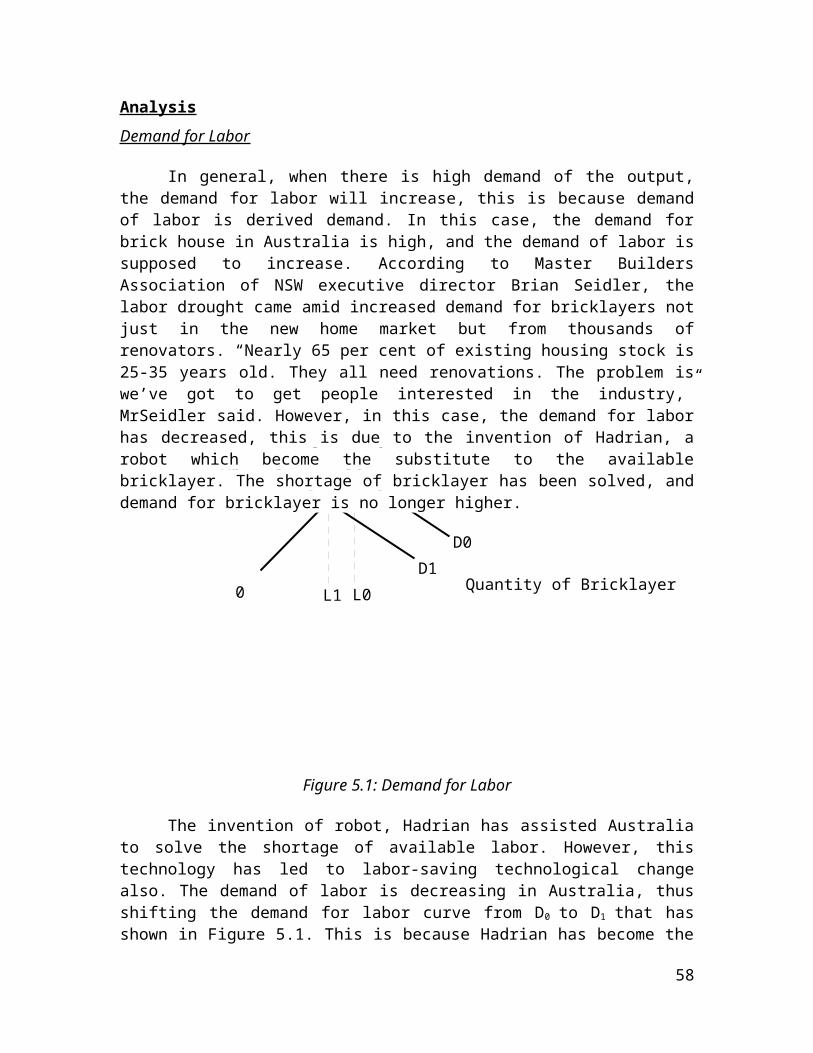
Once again the government can correct the market failure by inducing market participants to internalize the externality. The appropriate response in the case of positive externalities is exactly the opposite to the case of negative externalities. To move the market equilibrium closer to the social optimum, a positive externality requires a subsidy. Health and medication are heavily subsidized through public hospital.

Negative externality

A negative externality (also called "external cost" or "external diseconomy") is an economic activity that imposes a negative effect on an unrelated third party for which they are not compensated. In this case, the market has failed because no one pays for the cost resulting from negative externalities. It can arise either during the production or the consumption of a good or service. Externalities commonly occur in situations where property rights over the assets or resources have not been allocated, or are uncertain. For example, no one owns the oceans and they are not the private property of anyone, so ships may pollute the sea without fear of being taken to court.

Government can correct these market failures. A variety of approaches can be used to address the problem of negative externalities. For example, the government can impose a pollution compensation tax on an activity that creates negative externalities in order to bring the private cost in line with the social cost of the activity. Creating new property forms is another alternative. Here, instead of government directly regulating an activity to make sure that resources are allocated efficiently, resources may be privatized so that the individuals will have an incentive to exercise property rights to the resources efficiently. Or, the government may impose obligatory controls regarding certain activities. For example, most municipalities do not allow leavers to be burned or dogs to roam freely.

58

Supply (Private Cost)

0 QoptimumQmarket

Price of Water

Demand (Private Value)

Social Cost (Private Cost and External Cost)

Optimum

Equilibrium

Quantity of Water

Analysis

Scarcity

Water is the resource that is scarce in this article. The reason being overconsumption of water and water pollution. The natural resource of water is not enough to cover the high consumption of our society. Therefore in order to solve the problem, the authorities have urged public and private sectors to invest in programs that protects water supplies.

Different types of goods

Water, like public goods, is not excludable. The water consumption of one does not hinder the other person from using it. It is, however, rivalrous in consumption. When one consumes water, it precludes the consumption of water by another person. Therefore, water is a common resource. While public goods are free of charge to anyone that uses them, it is not the same for common resources. To prevent overuse of water, the government has imposed usage charges to mitigate the problem. As the market for water does not adequately protect the environment, the contamination caused by the markets are remedied with regulations, fee imposition or with corrective taxes on polluting activities. Therefore, water is a common resource.

Externalities

Figure 7.1: Pollution and Social Optimum

Due to externality, the cost to society of producing clean water is larger than the cost for the firm to manufacture it. For each unit of goods is to be developed, the social cost which includes the individual costs of the goods producers plus the cost to those bystanders affected adversely by the pollution of water. From the Figure 7.1 above depicts the societal price of producing commodities. The social-cost curve is above the

59

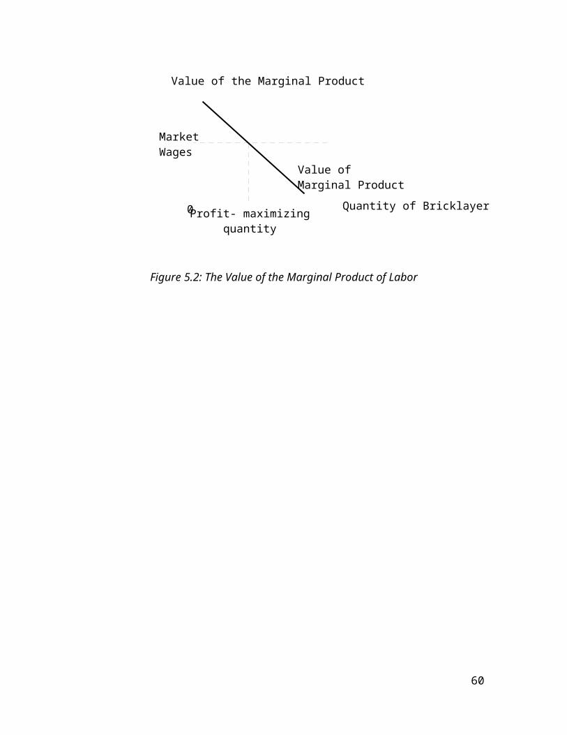
supply curve because it brings into account the external cost imposed on society by goods producers. The difference between these two curves reflects the cost of the pollution emitted.

To determine what quantity of clean water should be produced, a benevolent planner will require to maximize the total surplus derived from the market (the value to consumers of goods minus the price of making commodities). The planner will understand that the cost of producing clean water includes the extraneous costs of the pollution. Thus, it is rational to choose the level of resource produced at which the demand curve crosses the social-cost curve. This intersection determines the optimal quantity of clean water from the societal point of view.

It is observed that the balance amount of goods, Qmarket, is bigger than the socially optimal quantity, Qoptimum. The understanding of this inefficiency is that the market equilibrium reflects only the private cost of output. In the market equilibrium, the marginal consumer values goods less than the social cost of producing it. That is, at Qmarket, the demand curve lies below the social-cost curve. Therefore, reducing clean water production and consumption under the market equilibrium level raises total economic welfare.

To achieve the optimal outcome, taxes should be imposed on industries that pollute the water supply. The function of such a tax, called internalizing the externality will give buyers and sellers in the market an incentive to take account of the external effects of their actions. The industry will take account on the cost of pollution when deciding how much output is to be produced. As the market price would reflect the tax on producers, consumers will have the incentive to consume a smaller quantity of water.

Conclusion

In conclusion, water is a common resource. It is scarce due to overconsumption and water pollution. Negative externalities arise due to industrialization leading to pollutants being emitted into the water source. Thus, government should impose taxes in order to prevent overconsumption and water shortage in the future.

60

APA Reference

Griffin, A. (2015). Hadrian the robot bricklayer can build a whole house in two days. Retrieved from http://www.independent.co.uk/life-style/gadgets-and-tech/news/hadrian-the-robot-bricklayer-can-build-a-whole-house-in-two-days-10347229.html

Huffman, T. (2015). Corn yields up, prices down. Retrieved from http://www.effinghamdailynews.com/news/farm_fair_2015/corn-yields-up-prices-down/article_efe25caa-359b-11e5-bf24-6b856d5d6065.html

J.Holzer, H. (2015).A $15-hour minimum wage could harm America’s poorest workers. Retrieved from http://www.brookings.edu/research/opinions/2015/07/15-dollar-minimum-wage-harm-economy-holzer

Keene, N. (2015). Huge Demand for Brickies: Much moolah to be had for willing workers. Retrieved from http://www.dailytelegraph.com.au/news/nsw/huge-demand-for-brickies-much-moolah-to-be-had-for-willing-workers/story-fni0cx12-1227245387308

Scott, C. (2015). FAO urges sustainability over immediate profits to safeguard water supplies. Retrieved from http://www.foodnavigator.com/Policy/FAO-urges-sustainability-over-immediate-profits-to-safeguard-water-supplies

Wan IlaikaMohdZakaria. (2015). Honda: Car prices to fall post-GST. Retrieved from http://www.thesundaily.my/news/1303673

Zatlin, A. (2015). Americans Are Having Fun (And Spending). Retrieved from

http://www.benzinga.com/economics/15/08/5781095/americans-are-having-fun-and-spending

61

Marking Scheme

Marking Scheme Marks

Summary of the newspaper cutting

Discussion (Introduction, Theory, Concept etc)

Appropriate diagrams, explanation of the diagrams and application

Conclusion

References

English competency

Total

62