Embed Size (px)
Citation preview
Forschungsinstitut zur Zukunft der ArbeitInstitute for the Study of Labor
DI
SC
US
SI
ON
P
AP
ER
S
ER
IE
S
Poor Little Rich Kids? The Determinants of the Intergenerational Transmission of Wealth
IZA DP No. 9227
July 2015
Sandra E. BlackPaul J. DevereuxPetter LundborgKaveh Majlesi
Poor Little Rich Kids? The Determinants of the
Intergenerational Transmission of Wealth
Sandra E. Black University of Texas at Austin, NHH, IZA and NBER
Paul J. Devereux
University College Dublin, CEPR and IZA
Petter Lundborg
Lund University, IZA and CED Lund
Kaveh Majlesi Lund University, KWC
Discussion Paper No. 9227 July 2015
IZA
P.O. Box 7240 53072 Bonn
Germany
Phone: +49-228-3894-0 Fax: +49-228-3894-180
E-mail: [email protected]
Any opinions expressed here are those of the author(s) and not those of IZA. Research published in this series may include views on policy, but the institute itself takes no institutional policy positions. The IZA research network is committed to the IZA Guiding Principles of Research Integrity. The Institute for the Study of Labor (IZA) in Bonn is a local and virtual international research center and a place of communication between science, politics and business. IZA is an independent nonprofit organization supported by Deutsche Post Foundation. The center is associated with the University of Bonn and offers a stimulating research environment through its international network, workshops and conferences, data service, project support, research visits and doctoral program. IZA engages in (i) original and internationally competitive research in all fields of labor economics, (ii) development of policy concepts, and (iii) dissemination of research results and concepts to the interested public. IZA Discussion Papers often represent preliminary work and are circulated to encourage discussion. Citation of such a paper should account for its provisional character. A revised version may be available directly from the author.
IZA Discussion Paper No. 9227 July 2015
ABSTRACT
Poor Little Rich Kids? The Determinants of the Intergenerational Transmission of Wealth1
Wealth is highly correlated between parents and their children; however, little is known about the extent to which these relationships are genetic or determined by environmental factors. We use administrative data on the net wealth of a large sample of Swedish adoptees merged with similar information for their biological and adoptive parents. Comparing the relationship between the wealth of adopted and biological parents and that of the adopted child, we find that, even prior to any inheritance, there is a substantial role for environment and a much smaller role for genetics. We also examine the role played by bequests and find that, when they are taken into account, the role of adoptive parental wealth becomes much stronger. Our findings suggest that wealth transmission is not primarily because children from wealthier families are inherently more talented or more able but that, even in relatively egalitarian Sweden, wealth begets wealth. JEL Classification: G11, J01, J13, J62 Keywords: intergenerational mobility, nature versus nurture, portfolio allocation Corresponding author: Sandra E. Black Department of Economics University of Texas at Austin 1 University Station #C3100 Austin, TX 78712 USA E-mail: [email protected]
1 The data used in this paper come from the Swedish Interdisciplinary Panel (SIP) administered at the Centre for Economic Demography, Lund University, Sweden.
2
1. Introduction
Wealth inequality has increased dramatically in recent decades. Indeed, a
recent study found that, in the U.S., the median net worth of upper-income families
doubled in a 30-year period, but declined for lower-income families.2 This fact, in
conjunction with the release of Thomas Piketty’s Capital in the 21st Century that
highlights the intergenerational transmission of wealth as a key determinant of the
nature of society more generally, has brought renewed interest in understanding the
determinants of the intergenerational correlation in wealth (Piketty 2014).
Given this, it is surprising how little we know about the nature of
intergenerational correlations in wealth. While there are many studies about
intergenerational transmission of education and income, much less is known about
wealth, despite the fact that wealth is probably a better measure of economic success
than income or education and is more easily transferred across generations. 3
Importantly, wealth is also much less equally distributed than education and income.
There have been a number of recent papers that have generated estimates of the
intergenerational correlation of wealth. Charles and Hurst (2003) use U.S. data and
find elasticities of about 0.37 for net wealth.4 More recently, Boserup, Kopczuk, and
Kreiner (2014) and Adermon, Lindahl, and Waldenström (2015) have used register data
(from Denmark and Sweden, respectively) to estimate multi-generational models of
wealth transmission and found strong positive intergenerational rank correlations.5
But why is wealth correlated across generations? Is it nature or nurture? There
2 http://www.pewresearch.org/fact-tank/2014/12/17/wealth-gap-upper-middle-income/ 3 See Black and Devereux (2011) for a survey of the literature on intergenerational mobility. 4 See also Pfeffer and Killewald (2015) for a re-analysis using updated PSID data. 5 Also noteworthy, Clark and Cummins (2014) use rare surnames and estate records to show strong transmission of wealth in England over many generations.
3
is very little work examining the underlying causes of these correlations.6 One possible
pathway is through biology-- genetic inheritance of skills, attitudes, and preferences
that correlate with higher wealth in each generation.7 Another pathway is environment-
-wealthier parents may invest more in their children’s human capital, help their children
get better jobs, provide funding for business start-ups, or give financial gifts. In this
paper, we attempt to disentangle the role of nature versus nature in the intergenerational
transmission of wealth.
The nature/nurture distinction is important as it distinguishes between
fundamentally different reasons for positive intergenerational wealth correlations. The
nature or genetic channel suggests that these correlations can arise because children
from wealthy families are inherently more talented and would be wealthier than others
even without the advantage of growing up with wealthy parents. The nurture or
environmental channel instead suggests that parental wealth enables children to acquire
greater wealth either directly through inheritance or indirectly through human capital
investments or other environmental influences. The distinction is of great importance
for policy and for our perspective on the intergenerational correlation.8
To provide insight into this issue, we take advantage of a unique feature of the
Swedish adoption system whereby we observe both the biological and adoptive parents
of adopted children. We use administrative data on the net wealth of a large sample of
adopted children born between 1950 and 1970 merged with similar information for
6 A related literature has examined the genetic contribution to different components of wealth by comparing fraternal and identical twins. Using this strategy, Cronqvist and Siegel (2015) argue that genetic differences explain a substantial fraction of the variation in savings propensities and wealth at retirement. Barnea, Cronqvist, and Siegel (2010) find that one-third of the variation in the share in equities in financial portfolios is explained by a genetic effect. 7 Evidence on genetic effects in risk aversion and risk-taking behavior is found in Cesarini et al. (2010), Kuhnen and Chiao (2009), Dreber et al. (2009), and Black et al. (2015). 8 For example, a tax on parental wealth is likely to have less implication for intergenerational mobility if the intergenerational wealth correlation is predominantly due to nature rather than nurture.
4
their biological and adoptive parents--as well as corresponding data on own-birth
children. We disentangle the role of nature versus nurture in the intergenerational
transmission of wealth by looking at how the wealth of adoptive children is related to
that of both their biological and adoptive parents. Adoption allows us to examine the
effects of environmental factors in a situation where children have no genetic
relationship with their (adoptive) parents.
We find that, even before any inheritance has occurred, wealth of adopted
children is more closely related to the wealth of their adoptive parents than to that of
their biological parents. This suggests that wealth transmission is primarily due to
environmental factors rather than because children of wealthy parents are inherently
more talented. We also examine the role played by bequests and find that, when they
are taken into account, the role of adoptive parental wealth becomes much stronger.
The structure of the paper is as follows. In the next section, we discuss the
institutional background both in terms of financial markets and the adoption process. In
section 3, we outline the econometric methodology and, in section 4, we describe the
data. Section 5 provides our estimates for the intergenerational transmission of wealth.
In Section 6, we discuss a variety of robustness checks, including tests for non-random
assignment of adoptees, the effects of varying the age of measurement of wealth, and
different measures of net wealth. Section 7 then discusses our findings and concludes.
2. Institutional Background
A. Wealth in Sweden
Non-retirement wealth in Sweden is principally held in real assets--primarily
housing--and financial wealth, including cash, stocks, and bonds. While we do not have
information on pension wealth, non-retirement wealth accounts for almost 84 percent of
5
aggregate household financial wealth and a much higher proportion of total wealth.9
However, it is important to understand the nature of the pension system due to its
potential effect on savings.
Relative to countries such as the U.S., Sweden’s pension system would be
considered quite generous. Sweden has a mix of public and private pension schemes,
and individuals are allocated to different pension systems depending on the public or
private sector affiliation and year of birth of the individual. The longer one works, the
higher the pension one receives. The retirement age is flexible and individuals can
claim retirement benefits beginning at age 61.10
Because we study the individual wealth of children, it is important to understand
whether there are incentives to transfer wealth holdings from one spouse to another.
There do not appear to be any such incentives. In the event of a divorce, in the absence
of a prenuptial agreement, all assets are split equally among spouses. For wealth tax
purposes, the value of jointly owned assets was split evenly between the two tax filers.
Thus, there were no incentives for husbands and wives to strategically allocate assets
between themselves in order to reduce their wealth tax bill.
9 See Calvet, Campbell, and Sodini (2007). Also, stock market participation rates are higher in Sweden than in many other countries such as the United States (Guiso, Haliassos, and Jappelli, 2001). 10 In 1999, when we measure wealth of parents, the public pension system almost entirely consisted of a national pension plan financed on a pay-as-you-go basis (an individual account system known as the Premium Pension System (PPS) was introduced in 1999). In addition, most people receive an occupational pension from their employer. According to the Swedish Pensions Agency, about 90% of employees receive some pension benefits from their employer as a condition of employment. On average, around 4.5% of the employee's salary is put into employer provided schemes (Thörnqvist and Vardardottir, 2014). Swedish residents also have tax incentives to invest in private pension savings that are only accessible after retirement. However, as mentioned earlier, individuals still hold a substantial fraction of their wealth in non-retirement wealth. There is also a guaranteed pension for those who have had little or no income from work, and the size of this guaranteed pension is based on how long the person has lived in Sweden. In 2000, the maximum guaranteed pension, which applies to those who have lived in Sweden for at least 40 years, is 2394 SEK per month ($254) before taxes for those who are married, and 2928 SEK per month ($311) for a single person. A tax rate of 30 percent is then applied.

6
B. The Adoption System11
The adoptees we study were born between 1950 and 1970. During this period,
private adoptions were illegal, so all adoptions went through the state. The state
collected information on both the biological and adoptive parents; while it only required
information on the biological mother, in many cases, social workers were also able to
identify the biological fathers. While we do not observe how old the children were
when they were adopted, about 80% of children were adopted in their first year of
life.12
In order to adopt a child, a family had to satisfy certain requirements. The
adoptive parents had to be married and be at least 25 years old, have appropriate
housing, and be free of tuberculosis and sexually transmitted diseases. The adoptive
father was required to have a steady income and the adoptive mother was required to be
able to stay home with the child for a certain period of time.13 Overall, the adoption
criteria meant that the adoptive parents were positively selected relative to the general
population.
While matching of children to adoptive parents was at the discretion of the
caseworkers, the evidence from that period suggests that social authorities were not
able to systematically match babies to families based on family and child characteristics
(see Lindquist, Sol, and Van Praag 2015 for more details). However, we will examine
this issue in more detail later.
11 See Bjorklund, Lindahl, and Plug (2006) and Lindquist, Sol, and Van Praag (2015) for more details. 12 Upon turning 18, an adopted child has the legal right to obtain information from public authorities about the identity of his or her biological parents (Socialstyrelsen 2014). However, according to Swedish law, there is no legal requirement for parents to inform adopted children that they are adopted (SOU 2009). 13 Prior to 1974, there was no parental leave to care for adopted children. However, from 1955, mothers of biological children had a right to 3 months of paid leave (SOU 1954).
7
3. Empirical Strategy
A large body of literature in economics has used data on adoptees to disentangle
the relative contribution of genes and environment to economic behavior. These studies
have typically used information on foreign-born adoptees, where the characteristics of
the biological parents are unknown to the researcher. These studies have therefore not
been able to compare the relative influence of biological and adoptive parents.14
However, a recent literature has taken advantage of the unique Swedish register
data that identify both biological and adoptive parents. The first was the seminal study
by Björklund, Lindahl, and Plug (2006), who studied the relative roles of nature versus
nurture in the intergenerational transmission of educational attainment and earnings.
This was followed by papers using a similar strategy to study voting behavior (Cesarini,
Johannesson, and Oskarsson, 2014), crime (Hjalmarsson and Lindquist, 2013),
entrepreneurship (Lindquist, Sol, and Van Praag, 2015), health (Lindahl et al. 2015),
and risk-taking in financial markets (Black et al. 2015). In general, these studies have
found evidence that both characteristics of biological and adoptive parents are
predictive of child outcomes.
Our main variable of interest is net wealth, which is constructed by subtracting
total debts from total wealth. We transform the measure of net wealth in various ways
in our empirical analyses. As our primary variable of interest, we construct within-
cohort measures of parents’ and children’s rank within the wealth distribution. As
discussed in more detail later, we base this choice on the fact that the relationship
14 While working on this paper, we became aware of concurrent work by Fagereng, Mogstad, and Rønning (2015), who use Korean adoptees in Norway to determine the effect of environment on child wealth and asset allocation. The authors find a substantial role for environment. A key advantage of this work is that the assignment of children to families is arguably random. A key limitation, however, is that they do not observe characteristics of the biological family. We view this paper as a complement to our own work. More broadly, see Sacerdote (2010) for a survey of this literature.
8
between child’s rank and parent’s rank is approximately linear. However, we also test
the sensitivity of our conclusions to the choice of an inverse hyperbolic sine
transformation of net wealth, as well as the untransformed value of net wealth (in
levels).
Our main specification relates the rank of net wealth of an adoptee to the rank of
net wealth of both his/her biological and adoptive parents. We estimate the following
equation:
𝑊!" = 𝛽! + 𝛽!𝑊! + 𝛽!𝑊! + 𝑋𝛽! + 𝜖!" (1)
where W, our main variable of interest, is the rank of net wealth, i indexes the
biological family, j indexes the adoptive family, and X refers to the set of control
variables. These include year-of-birth dummies for both parents and children and a
dummy variable for the gender of the child. We measure child wealth at the individual
level but measure parental wealth as the average of the mother’s and father’s wealth.
For each child, we compute his/her rank in the distribution of child wealth for
individuals born in the same year and so measured at the same age. Within an age
cohort, ranks are normalized to lie between 0 and 100.15 We use the child’s rank in the
entire distribution (of their cohort) throughout the analysis even when we are studying
subgroups of children such as the sample of adoptees. We carry out the same exercise
for parental wealth basing the cohort on the average cohort of the two parents.
A key assumption of our empirical strategy is that adoptees are randomly
assigned to adoptive families at birth. If this assumption holds, the coefficients on the
wealth of biological parents provide an estimate of the effect of pre-birth factors and the
coefficient of adoptive parents provide an estimate of the effects of post-birth factors.
The assumption will be violated if adoptees are systematically matched to adoptive
15 Ranks are calculated as [(𝑖 − 0.5)/𝑁] ∗ 100 where i denotes individuals sorted by wealth, and i = 1,2, . . . , N.
9
parents that are similar to their biological parents. To test this assumption, we will
conduct a battery of robustness checks, where we provide evidence suggesting that any
violations of the assumption do not invalidate our estimates.
4. Data
We construct our database by merging a number of administrative registers. Our
starting point is an administrative dataset containing information on all Swedish
citizens born between 1932 and 1980. These data include information on educational
attainment, county of residence, and other basic demographic information.16 To this, we
merge data from the Swedish multigenerational register, where we are able to identify
Swedish-born adoptees by using information on both biological and adoptive parents of
children.17
Our data on wealth come from the Swedish Wealth Data
(Förmögenhetsregistret). These data were collected by the government’s statistical
agency, Statistics Sweden, for tax purposes between 1999 and 2007, at which point the
wealth tax was abolished.18 For the years 1999 to 2006, the data include all financial
16 We impute years of schooling based on the information on highest educational degree completed contained in the education register. We follow the coding of Holmlund, Lindahl, and Plug (2011) and impute years of schooling in the following way: 7 for (old) primary school, 9 for (new) compulsory schooling, 9.5 for (old) post-primary school (realskola), 11 for short high school, 12 for long high school, 14 for short university, 15.5 for long university, and 19 for a PhD university education. Since the education register does not distinguish between junior-secondary school (realskola) of different lengths (9 or 10 years), it is coded as 9.5 years. For similar reasons, long university is coded as 15.5 years of schooling. 17 We know the identity of biological fathers for only about 50% of adoptees. While we cannot directly examine the sensitivity of our estimates to this issue because our parental variable is measured at the family level, previous studies that examined mother characteristics and behavior have found no evidence of bias due to missing fathers. See Black et al. (2015) and Lindqvist et al. (2015). 18 During this time period, the wealth tax was paid on all the assets of the household, including real estate and financial securities, with the exception of private businesses and shares in small public businesses (Calvet, Campbell, and Sodini 2007). In 2000, the tax rate was 1.5 percent on net household wealth exceeding SEK 900,000. The Swedish krona traded at $0.106 at the end of 2000, so this threshold corresponds to $95,400. After 2000, the tax threshold was raised to SEK 1,500,000 for married couples and non-married cohabitating couples with common children and 1,000,000 for single taxpayers. In 2002 the threshold rose again, this time to SEK 2,000,000 for married couples and non-married cohabitating
10
assets held outside retirement accounts at the end of a tax year, December 31st, reported
by a variety of different sources, including the Swedish Tax Agency, welfare agencies,
and the private sector. Financial institutions provided information to the tax agency on
their customers’ security investments and dividends, interest paid or received, and
deposits, including nontaxable securities and securities owned by investors, even for
persons below the wealth tax threshold. Because the information is based on statements
from financial institutions, it is likely to have very little measurement error, and
because the entire population is observed, selection bias is not a problem.19
From the wealth register, we observe different categories of wealth. This
includes the aggregate value of bank accounts, mutual funds, stocks, options, bonds,
housing wealth, and capital endowment insurance as well as total financial assets and
total assets.20 The wealth register also contains data on total debt and net wealth.
Nonfinancial assets are collected from the property tax assessments and valuations are
based on market prices.21
We measure income for our sample by using data from the Swedish Income
Register. The register contains yearly income from 1968 onwards, and we use a
measure of income that includes earnings from employed labor as well as self-
employment income and taxable benefits.
couples and 1,500,000 for single taxpayers. In 2005 the threshold rose once more but this time only for married couples and cohabitating couples, this time to SEK 3,000,000. 19 In the case of foreign assets, individuals were required to report these themselves. Evidence suggests that unreported foreign assets likely represent a small fraction of total household assets. (Calvet, Campbell, and Sodini 2007) 20 Small bank accounts were not reported by banks to the Swedish Tax Agency unless there was more than 100 SEK (about $10) in interest during the year. However, Statistics Sweden estimates that 98% of the total money in bank accounts is included in the data. 21 Statistics Sweden adjusts tax-assessed property values using information on both tax assessments and actual sales prices of houses so the aggregate value of the housing stock in the data is consistent with sales prices (Adermon et al. 2014).
11
We limit our analyses to children born 1950-1970 with all applicable parents
alive in 1999 and for whom we have information on schooling, earnings, and wealth. In
our analyses, we measure net wealth of the children in 2006 and net wealth of the
parents in 1999. In order to avoid the issue of inheritances, we further restrict that at
least one parent is alive in 2006 (for adoptees, we require that at least one adoptive
parent be alive in 2006); however, we later test the sensitivity of our conclusions to this
choice. The logic for restricting our sample to children born by 1970 and measuring
their wealth in the latest possible year, 2006, is to avoid having very young people in
the sample who have not yet had much opportunity to accumulate wealth. The average
age of children in our sample is 44. This compares with an average age of 38 in Charles
and Hurst (2003), 47 for the third generation in Adermon et al. (2015), and 34 for the
second generation in Boserup et al. (2014). Later, we show that our estimates are not
sensitive to the exact ages of the children at wealth measurement.
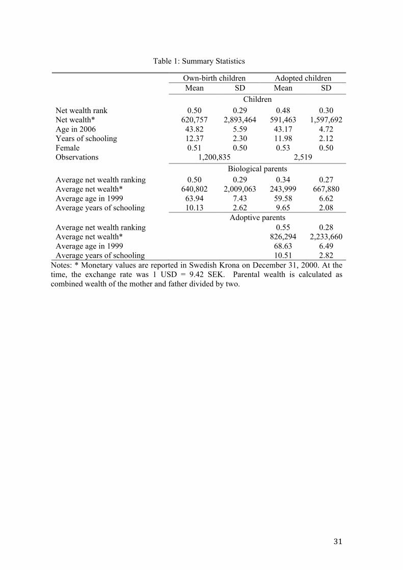
We have information on over 1.2 million children who are raised by their
biological parents and 2519 adopted children for whom we have data available for both
biological and adoptive mothers and fathers. Descriptive statistics for our sample are
shown in Table 1. In the top panel, we show means for children, both biological and
adoptive. In 2006, when their assets and education are measured, the average child age
is 44 for biological children and 43 for adoptive children. On average, biological
children have 0.4 of a year more education and hold slightly higher net wealth (621K
SEK vs. 591K SEK).
In the second panel, we show means for biological parents, both parents who
raised their own biological children and parents who gave their children up for
adoption. The two types of parents are quite different in their characteristics, with
biological parents of adoptees being much less wealthy and having fewer years of
12
schooling.
The bottom panel of Table 1 shows descriptive statistics for adoptive parents.
For adopted children, adoptive parents are, on average, older, wealthier, and better
educated than the child’s biological parents. Adoptive parents also appear positively
selected when we compare them to biological parents who raise their own children,
although the differences here are much smaller.22
5. Results
When considering the intergenerational correlation in wealth, the literature is
agnostic as to the appropriate functional form. Research in the area has used a variety
of transformations of net wealth, including levels, logs, the inverse hyperbolic sine
transformation, and within cohort ranks. When we examine the data, it is clear that the
within-cohort rank specification best fits the linear model; as a result, we use that as our
preferred specification. However, in later analyses, we will show that our conclusions
are robust to the choice of the measure of net wealth.
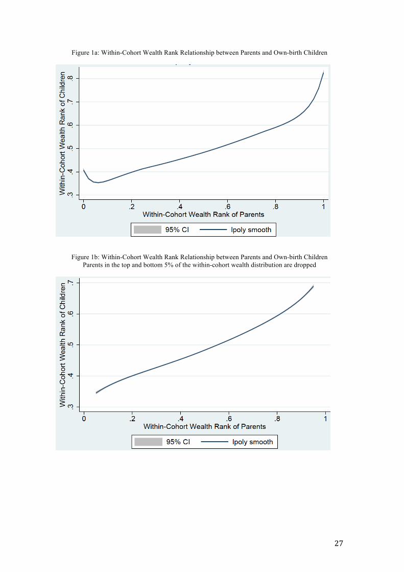
Figure 1a plots the relationship between the within-cohort rank of net wealth of
parents and children for the large own-birth sample using a local linear kernel
regression with an epanechnikov kernel and rule-of-thumb bandwidth.23 Importantly,
we see that this relationship is approximately linear from around the 5th percentile to the
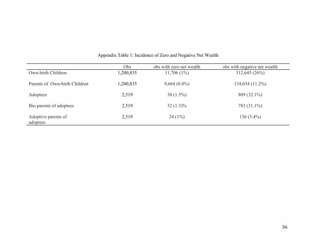
22 Appendix Table 1 provides a breakdown of the proportions of sample members who have positive, zero, and negative net wealth respectively. In the sample of own-birth children, almost 1% have zero net wealth, and 26% have negative wealth. For adoptive children, the percentages are 1% and 32%. As discussed by Boserup et al. (2015), standard life-cycle theory would predict negative wealth for young persons with increasing earnings profiles. Unsurprisingly, the proportions with zero and negative wealth are lower for parents, both because they are older and because we are averaging wealth across the father and the mother. Among parents of own-birth children, 11.1% have negative wealth and 1% have zero net wealth. The percentages with negative wealth are 5% for adoptive parents and 31% for biological parents of adoptees. This provides further evidence that biological parents of adoptees are negatively selected. 23 Adermon et al. (2015) also use this approach. An alternative, used by Boserup et al. (2014), is to plot average child rank against parental wealth percentile. The local linear kernel regression is more efficient and this is important given our sample of adoptees is not very large.
13
95th percentile. Consistent with the Swedish findings of Adermon et al. (2015), the
slope is negative at the very bottom of the distribution and more steeply positive at the
top. The declining slope at the bottom is driven by parents with large negative wealth.
The increase in slope at the top is consistent with general findings of greater persistence
in economic status at the very top of the distribution (Björklund et al. 2012). Figure 1b
shows the equivalent picture when we drop the parents in the top and bottom 5% of
their within-cohort distribution, and the linearity of the relationship becomes more
pronounced.24
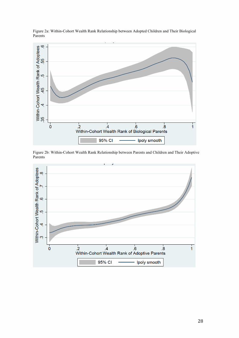
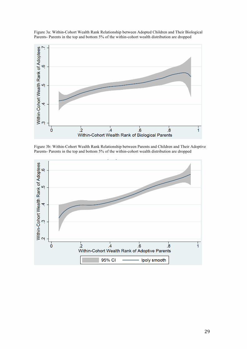
Among adopted children, Figures 2a and 2b plot the within-cohort rank
relationship between children and biological and adoptive parents respectively. Here,
we see similar patterns to the full sample. However, confidence intervals become much
wider at the tails, and this is more pronounced at the top of the distribution among
biological parents and at the bottom of the distribution among adoptive parents. This
highlights the fact that biological parents are primarily negatively selected in terms of
net wealth while adoptive parents are positively selected. When we trim the top and
bottom 5% of the data, the relationship again becomes much more linear. (Figures 3a
and 3b).
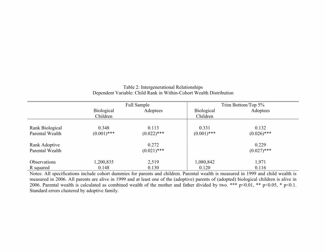
In Table 2, we report the regression results when we estimate equation (1) on
the sample of own-birth children (Columns 1 and 3) and adoptees (Columns 2 and 4).
As noted earlier, we include cohort dummies for parents and children in all
specifications.25
Columns 1 and 2 present the rank-rank coefficient for own-birth and adopted
24 In this case, we rank all individuals within a given cohort (for parents, we calculate the cohort as the rounded average of the father and mother) and trim the top and bottom 5%. As a result, adoptive parents, biological parents, and own-birth parents in the same cohort are all ranked within the same distribution. 25 Given wealth is measured in the same year for all parents and wealth is measured in the same year for all children, these also serve as age dummies. The estimates without these dummies are quite similar. This is what we would expect for the rank transformation as the ranks are computed by cohort.

14
children, respectively. In the case of adopted children we control for the within-cohort
rank of the net wealth of biological parents as well as that of adoptive parents. Among
own-birth children (Column 1), the rank-rank coefficient is approximately 0.35.
Among adoptees (Column 2), we find that child's wealth is predominantly associated
with that of adoptive parents and has a much weaker relationship with biological
parents’ wealth. The rank coefficient for biological parent wealth is 0.11 but that for
adoptive parent wealth is 0.27.
We saw in Figures 1 and 2 that the rank-rank relationship is approximately
linear except in the tails of the parental wealth distribution -- for ranks up to the 5th
percentile and in the very top of the distribution. Therefore, in Columns 3 and 4, we
drop cases with parental wealth in the top or bottom 5 percentiles of the within-cohort
parental wealth distribution. This is particularly important in the adoptive sample, as
biological parents are much poorer than adoptive parents. Not surprisingly, given the
figures earlier, these exclusions do affect our estimates, with an increase in the effect of
biological wealth and a decrease in the effect of adoptive wealth. Still, however, the
adoptive coefficient is substantially larger than the biological one. The relatively weak
relationship between biological parental wealth and child wealth is interesting as it
suggests that most of the reason for the intergenerational transmission of wealth is not
due to the fact that children from wealthier families are innately more talented. Instead,
it appears that, even in a relatively egalitarian society like Sweden, wealth begets
wealth.
We next consider whether these relationships are the same for sons and
daughters. We do not have a strong prior in terms of whether adoptive or biological
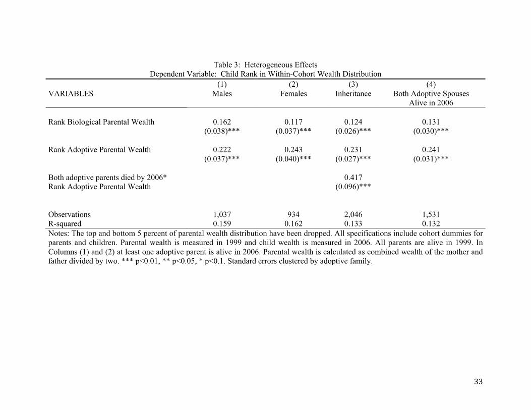
relationships should be stronger for boys or girls. In Table 3, we report the estimates
for our preferred specification where we exclude children whose biological or adoptive
15
parents have net wealth in the bottom or top 5% of the rank distribution. Columns 1 and
2 present the results by child gender. While the biological coefficient is larger for boys
than for girls, the difference is not statistically significant. The adoptive coefficient is
similar for both genders, suggesting there is not much evidence for gender differences
in the nature/nurture split.
Finally, we consider the potential role of inheritances when estimating
intergenerational correlations in wealth.26 In Sweden, as in the United States, when a
spouse dies their assets automatically transfer to the surviving spouse. Because we have
restricted the sample so that at least one parent in alive when child wealth is measured
in 2006, we are unlikely to have captured bequests. To test the potential role of
inheritances, we compare two extreme cases--in one, at least one parent was alive in
1999 but both parents are dead by 2006, suggesting that the child is likely to have
received inheritances in the interim, and in the other case, both parents are alive in both
periods, ruling out the possibility of inheritance. Column 3 of Table 3 presents the first
scenario; to estimate the potential effect of inheritances, we add a dummy variable for
whether both parents are deceased in 2006 plus an interaction of this dummy variable
with adoptive parental wealth.27 The estimates are in column (3) of Table 3. While we
have added only about 100 extra adoptive families to the sample, we still find a
statistically significant interaction effect of 0.42. This suggests that the rank correlation
with adoptive parent wealth increases from 0.23 to 0.65 once inheritances are included.
At the other extreme, we rule out the possibility that the child received an
inheritance by restricting the sample to cases with both adoptive parents alive in 2006.
26 Piketty and Zucman (2014, 2015) show that inheritance can have important effects on the distribution of wealth. Adermon et al. (2015) find that inheritance appears to be the most important component of the intergenerational wealth elasticity in Sweden. 27 We assume that biological parents of adoptive children will not have bequest motives for the children they gave up.
16
(Column 4) While this reduces the sample size considerably, the estimates are largely
unchanged from the baseline in Table 2 column 4. This is consistent with our
expectation that bequests to children occur after both parents die.
6. Robustness Checks
Random Assignment of Adoptees
As noted earlier, our identification strategy relies on the random assignment of
adoptees. However, even if adoptees are not randomly assigned to parents, we may be
able to test how this non-random assignment might be affecting our estimates. The
primary concern is that children may have been assigned to adoptive parents in such as
way that there are correlations between net wealth of adoptive (biological) parents and
unobserved characteristics of the biological (adoptive) parents that are correlated with
child wealth. While earlier work using similar identification strategies and data suggest
that this is unlikely to be a problem, we conduct a number of robustness checks to
verify this.
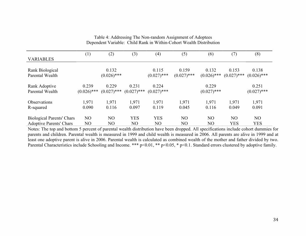
If there are correlations between the wealth of adoptive parents and unobserved
characteristics of the biological parents that are correlated with child wealth, the
coefficients on wealth of adoptive parents may be sensitive to whether or not the wealth
of biological parents is included in the regression. The results when we do this are
presented in Table 4.
Column 1 of Table 4 shows estimates with just the wealth of the adoptive
parents included.28 In column 2, we add wealth of the biological parents, which is the
specification previously reported in column 4 of Table 2. The coefficient on adoptive
parent wealth changes very little when we include biological parent wealth, suggesting
28 All specifications include cohort dummies for parents and children.
17
that the two variables are not highly correlated.
As another check for omitted variable bias, we next include a number of other
controls for characteristics of the biological parents; these include education and labor
income and are included separately for mothers and fathers.29 Column 3 of Table 4
includes wealth of adoptive parents and adds the further controls as proxies for general
unobserved characteristics of biological parents. Comparing the coefficients on
adoptive parent wealth in column 3 to column 1, again the difference is very small.
Finally, in column 4, we include both biological parents’ wealth as well as controls for
their schooling and income. The resulting estimates are almost identical to those in
column 3. Overall, it appears that our adoptive estimates are unlikely to be significantly
biased by non-random assignment.
Columns 5 to 8 of Table 4 carry out the analogous exercise for wealth of
biological parents. In column 5, we include only the wealth of biological parents and
then systematically add controls for characteristics of adoptive parents. Column 6
includes controls for the wealth of adoptive parents, Column 7 includes controls for
education and income (again entered separately for mothers and fathers), and Column 8
includes both sets of controls. While the coefficients on wealth of biological parents
decrease somewhat in columns 6-8 compared to column 5, the differences are not very
large. This suggests that non-random assignment of adoptees is unlikely to be a
problem and, if anything, will lead to an overstatement of the role of biological parents
relative to that of adoptive parents.
Ages at Measurement of Wealth
29 Our measure of biological parent earnings is calculated separately for mothers and fathers and is the log of average income between the years 1980 and 1999. In the very few cases where parental labor income is zero in all years, we set the log to zero
18
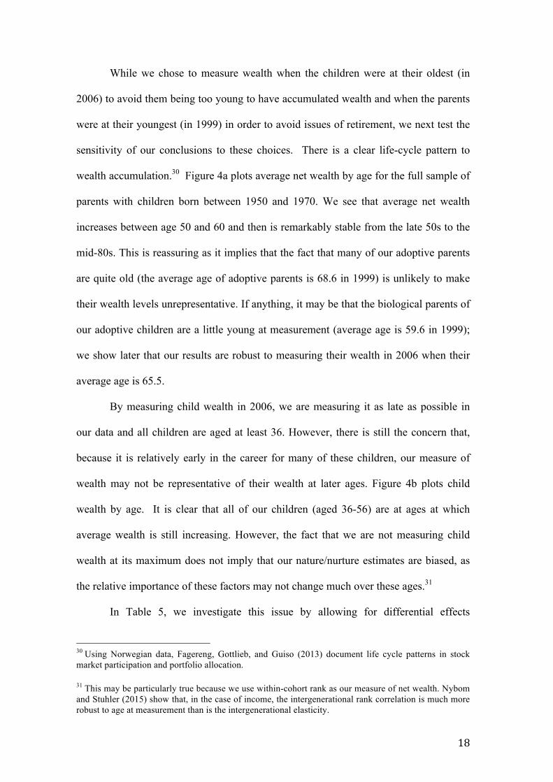
While we chose to measure wealth when the children were at their oldest (in
2006) to avoid them being too young to have accumulated wealth and when the parents
were at their youngest (in 1999) in order to avoid issues of retirement, we next test the
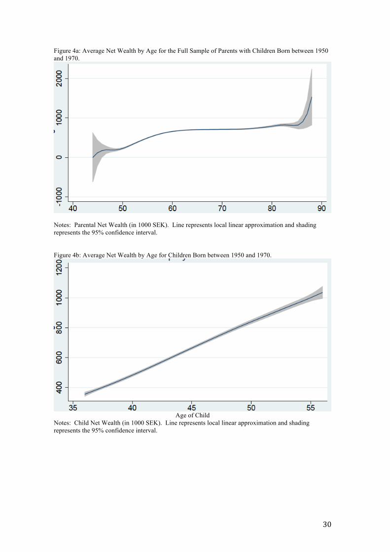
sensitivity of our conclusions to these choices. There is a clear life-cycle pattern to
wealth accumulation.30 Figure 4a plots average net wealth by age for the full sample of
parents with children born between 1950 and 1970. We see that average net wealth
increases between age 50 and 60 and then is remarkably stable from the late 50s to the
mid-80s. This is reassuring as it implies that the fact that many of our adoptive parents
are quite old (the average age of adoptive parents is 68.6 in 1999) is unlikely to make
their wealth levels unrepresentative. If anything, it may be that the biological parents of
our adoptive children are a little young at measurement (average age is 59.6 in 1999);
we show later that our results are robust to measuring their wealth in 2006 when their
average age is 65.5.
By measuring child wealth in 2006, we are measuring it as late as possible in
our data and all children are aged at least 36. However, there is still the concern that,
because it is relatively early in the career for many of these children, our measure of
wealth may not be representative of their wealth at later ages. Figure 4b plots child
wealth by age. It is clear that all of our children (aged 36-56) are at ages at which
average wealth is still increasing. However, the fact that we are not measuring child
wealth at its maximum does not imply that our nature/nurture estimates are biased, as
the relative importance of these factors may not change much over these ages.31
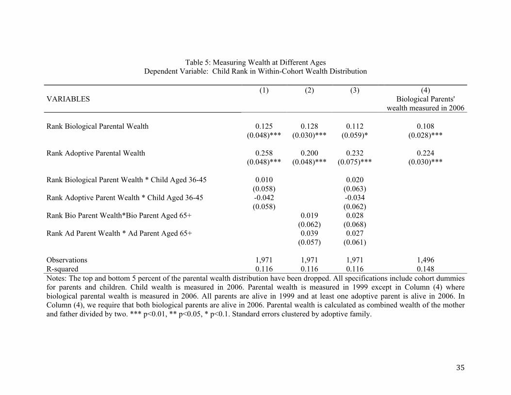
In Table 5, we investigate this issue by allowing for differential effects
30 Using Norwegian data, Fagereng, Gottlieb, and Guiso (2013) document life cycle patterns in stock market participation and portfolio allocation. 31 This may be particularly true because we use within-cohort rank as our measure of net wealth. Nybom and Stuhler (2015) show that, in the case of income, the intergenerational rank correlation is much more robust to age at measurement than is the intergenerational elasticity.
19
depending on the age at which wealth is measured. For children, we create a dummy
equal to 1 if they are born between 1961 and 1970 (and so aged between 36 and 45 at
wealth measurement and we interact this with wealth of both types of parents. We
include these interactions in Column 1; in this specification, the main effects can be
interpreted as the effects of parental wealth for children aged between 46 and 56 at
measurement. We see that the interaction effects are statistically insignificant and the
main effects are similar to those in Table 2 Column 4.32 This suggests that our
estimates are not sensitive to the age of child at wealth measurement.
In Column 2 of Table 5, we similarly test whether the coefficient estimates
depend on parental age at measurement. We define an older group of parents who are
aged 65 or older at measurement and we interact this with parental wealth. The main
effects can then be interpreted as the effects of parental wealth for the relatively young
parents. Once again the interaction terms are statistically insignificant and the main
effects are very similar to earlier estimates. In Column 3, we include interactions with
the age dummies for both parents and children and once again find insignificant
interaction terms. It appears that the relative contribution of nature and nurture is
largely invariant to the exact age at measurement of wealth of parents and children in
our sample.
Another potential issue is that biological parents are on average 9 years younger
than the adoptive parents in 1999 (average age of 59.6 versus 68.6). Given that there
are life-cycle patterns in wealth-holding, our conclusions may be sensitive to this
difference. To address this, we measure the wealth of adoptive parents in 1999 and
biological parents in 2006, thus largely eliminating the age gap at measurement.
Column 4 of Table 5 reports these estimates. Once again, we find that the estimates are 32 We have also tried interactions using a continuous child age variable and found the interactions to be small and statistically insignificant.
20
invariant to the age of measurement – the estimates in Column 4 are similar to our main
specification in Table 2 Column 4.
Different Transformations of Net Wealth
Thus far, we have used the within-cohort rank as our measure of net wealth—
from our own analysis, it is clear that this transformation fits the linear model the best.
However, we next test the sensitivity of our conclusions to this choice. In addition to
within-cohort rank, we consider the inverse hyperbolic sine transformation as well as
the level of net wealth.33
Charles and Hurst (2003) use a log transformation for both parent and child
wealth. However, this requires excluding all cases in which either parent or child has
zero or negative net wealth and many individuals have non-positive net wealth. To
avoid using a selected sample, we use the inverse hyperbolic sine transformation (IHS)
rather than logs.34 The IHS transformation of wealth, W, is 𝑤 = 𝑙𝑜𝑔 𝑊 + 𝑊! + 1
and behaves as log(𝑊) for positive values.35
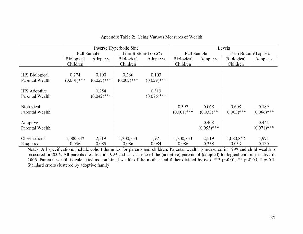
Appendix Table 2 presents the results when we estimate equation 1 using these
alternative measures of net wealth as our variables of interest. The IHS estimates for
own-birth children (Columns 1 and 3) suggest an intergenerational elasticity of about
0.28—the results are relatively constant whether the data are trimmed or not. Among
adoptees, we find similar patterns (Columns 2 and 4), with coefficients of .10 on
biological parents’ wealth and .25 on adoptive parents’ wealth, and these relative
33 Graphs of the relationship between parents and children’s net wealth using these alternative transformations do not, in fact, look linear; as a result, we chose to use the within-cohort rank as our preferred specification. These figures are available from the authors upon request. 34 The IHS is advocated by Pence (2006) as a superior alternative to using logs when studying wealth data. 35 We have verified in our data that the relationship between parent and child net wealth using the IHS is exactly the same as that using logs once all negative and zero values have been excluded.
21
patterns change little when we trim the data.
Columns 5-8 show the relationship between parental and child net wealth when
wealth is not transformed and is simply reported in levels. The levels estimate among
own-birth children is about 0.4 in the full sample but jumps to 0.6 when we exclude
wealth levels in the bottom and top 5% of the distribution of ranks (Columns 5 and 7).
This large change reflects the underlying non-linearities in the data. Finally, when we
consider adoptees, the adoptive parent coefficient is 0.41 and the biological coefficient
is 0.07 in the full sample; once we trim the data, the coefficient on biological parental
wealth almost triples to 0.19 compared with 0.44 for adoptive parental wealth. We
place little credence on the untrimmed estimates for the levels specification, however,
given the sensitivity to outliers. Overall, our conclusions of the relative importance of
adoptive parent’s wealth relative to that of biological parents are robust to the choice of
specification for net wealth.
Other Robustness Checks
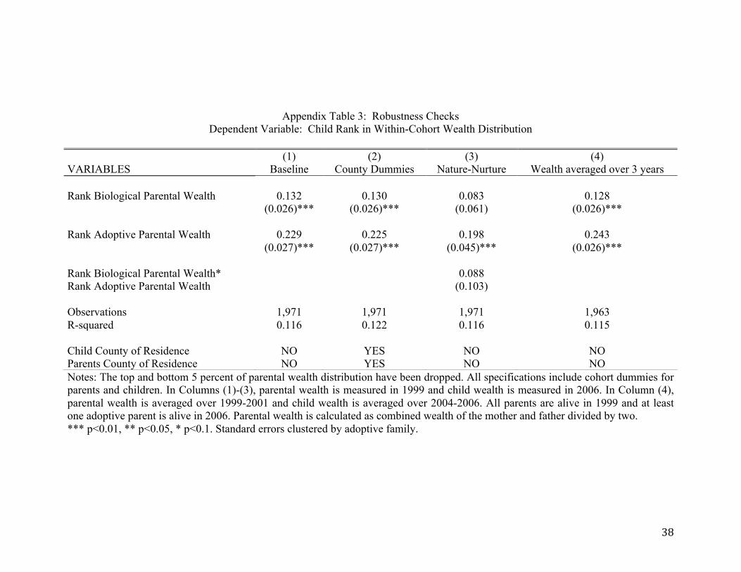
We report further robustness checks in Appendix Table 3. Column 1 presents
the baseline results from Table 2 Column 4 for comparison. In Column 2, we consider
whether our conclusions are sensitive to correlations between wealth and residence. It
may be that the wealth of parents and children are correlated because both live in an
area that has high wealth levels -- for example, they may both live in an area with high
property values. To examine this, in Column 2, we add controls for county of residence
of both parents and children in 2000.36 This has no effect on the estimates.
We have also thus far assumed that the effects of biological and adoptive
parents are independent of each other. However, this may be an oversimplification if 36 Sweden is divided into 20 regional county councils. Their main responsibilities are to provide and organize health care and public transportation.
22
there are nature/nurture interactions, one building on the other.37 We present the results
when we allow for an interaction between biological and adoptive parents in column (3)
of Appendix Table 3. The interaction term is positive but statistically insignificant and
so provides no evidence for a nature/nurture interaction.
Finally, while our wealth data are high quality and unlikely to suffer from
significant measurement error, there could be transitory shocks to wealth that lead our
estimates based on single years of wealth data to be misleading. Therefore, in column
(4) of Appendix Table 3, we measure child wealth as the average in 2004-06 and
parental wealth as the average over 1999-2001. We find that the averaging makes no
appreciable difference to the estimates.
7. Conclusions
There is an extensive body of research documenting a correlation in wealth
across generations, with little understanding of the underlying causes of this
relationship. Taking advantage of unique data from Sweden that link adopted children
to both their biological and adoptive parents, we are able to disentangle the role of
nature versus nurture in the intergenerational transmission of wealth.
We find a substantial role for environmental influences with a much smaller role
for biological factors, suggesting that wealth transmission is not primarily because
children from wealthier families are inherently more talented or more able. Instead, it
suggests that innate ability is only a small factor in this intergenerational relationship.
We also find that when bequests are taken into account the role of adoptive parental
wealth becomes much stronger. Importantly, our conclusions are robust to a variety of
37 There are mixed findings in the literature about these types of interactions – Bjorklund, Lindahl, and Plug (2006) finds evidence of these interactions for mothers' education and fathers' earnings but Lindquist, Sol, van Praag (2015) find no evidence for these interactions when studying entrepreneurship and Black et al. (2015) find no evidence for them when studying risky investment behavior.
23
specification and robustness checks.
While we have established the relative role of nature versus nurture, the exact
mechanisms of wealth transmission are more difficult to ascertain. Wealthier parents
tend to be better educated and earn higher incomes, and these factors could lead to the
increased wealth of their children, through, for example, teaching them about
investment opportunities or providing the right opportunities. However, when we
investigate this, we find little evidence that this is the case.38 It may also be that
wealthy parents invest more in their child’s education and career, which could then lead
to higher child wealth accumulation. When we examine whether this is the case,
however, we find little evidence for education or income as mechanisms.39 So, the
pathway through which parental wealth affects child wealth does not appear to be
primarily parental schooling and income or child human capital accumulation and
greater labor earnings. Taken together, our findings suggest potential roles for
intergenerational transmission of preferences (children of wealthier parents may choose
to save more or invest in assets that have higher returns) or for financial gifts from
parents to children. Unfortunately, we do not have information on savings behavior or
on financial gifts so this evidence is only suggestive.
It is clear from our results that innate childhood abilities do not drive the
intergenerational correlations in wealth we observe; however, more work is required to
determine the exact mechanisms through which wealthy parents create wealthy
children.
38 To investigate whether this can explain the patterns we observe, we have tried adding controls for adoptive parents’ education and income, including them separately for fathers and mothers. This had negligible effects on the coefficients on parental wealth, suggesting that adoptive parental wealth has a direct effect on child wealth that does not come through other parental characteristics. 39 We have examined the effects of parental wealth on child educational attainment and found the effect of adoptive parental wealth to be positive but small. Likewise, the effects of adoptive parental wealth on child labor earnings is modest and smaller than that of biological parents. Indeed, the effect of adoptive parental wealth on child wealth falls very little even when child education and labor earnings are introduced as additional controls.
24
References Adermon, A., Lindahl, M., & Waldenström, D. (2015). Intergenerational wealth mobility and the role of inheritance: Evidence from multiple generations. Unpublished manuscript. Barnea, A., Cronqvist, H., & Siegel, S. (2010). Nature or nurture: What determines investor behavior? Journal of Financial Economics, 98(3), 583-604. Björklund, A., Lindahl, M., & Plug, E. (2006). The origins of intergenerational associations: Lessons from Swedish adoption data. The Quarterly Journal of Economics, 999-1028. Björklund, A., Roine, J., and Waldenström, D. (2012). Intergenerational top income mobility in Sweden: Capitalist dynasties in the land of equal opportunity? Journal of Public Economics, 96: 474-484. Black, S. E., & Devereux, P. J. (2011). Recent developments in intergenerational mobility. Handbook of labor economics, eds. O. Ashenfelter and D. Card, 1487-1541. Amsterdam: Elsevier. Black S.E., Devereux, P.J., Lundberg P., and K. Majlesi (2015). On the Origins of Risk-Taking. NBER Working Paper #21332. Boserup, S. H., W. Kopczuk and C. Thustrup Kreiner (2014). Intergenerational Wealth Mobility: Evidence from Danish Wealth Records of Three Generations. Working Paper, University of Copenhagen. Calvet, L. E., Campbell, J. Y., & Sodini, P. (2007). Down or Out: Assessing the Welfare Costs of Household Investment Mistakes. Journal of Political Economy, 115(5), 707-747. Cesarini, D., Johannesson, M., Lichtenstein, P., Sandewall, Ö., & Wallace, B. (2010). Genetic Variation in Financial Decision-Making. The Journal of Finance, 65(5), 1725-1754. Cesarini, D., Johannesson, M., & Oskarsson, S. (2014). Pre-birth factors, post-birth factors, and voting: Evidence from Swedish adoption data. American Political Science Review, 108(01), 71-87. Charles, K. K., & Hurst, E. (2003). The Correlation of Wealth across Generations. Journal of Political Economy, 111(6). Clark, G. and N. Cummins (2014). Intergenerational Wealth Mobility in England, 1858–2012: Surnames and Social Mobility. Economic Journal 125(582): 61–85. Cronqvist, H., & Siegel, S. (2015). The Origins of Savings Behavior. Journal of Political Economy, 123(1), 123-169. Dreber, A., Apicella, C.L., Eisenberg, D.T.A., Garcia, J.R., Zamore, R.S., 2009. The 7R
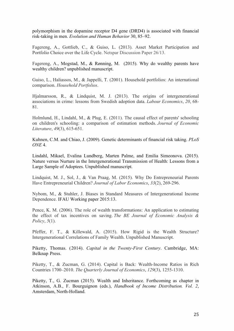
25
polymorphism in the dopamine receptor D4 gene (DRD4) is associated with financial risk-taking in men. Evolution and Human Behavior 30, 85–92. Fagereng, A., Gottlieb, C., & Guiso, L. (2013). Asset Market Participation and Portfolio Choice over the Life Cycle. Netspar Discussion Paper 26/13. Fagereng, A., Mogstad, M., & Rønning, M. (2015). Why do wealthy parents have wealthy children? unpublished manuscript. Guiso, L., Haliassos, M., & Jappelli, T. (2001). Household portfolios: An international comparison. Household Portfolios. Hjalmarsson, R., & Lindquist, M. J. (2013). The origins of intergenerational associations in crime: lessons from Swedish adoption data. Labour Economics, 20, 68-81. Holmlund, H., Lindahl, M., & Plug, E. (2011). The causal effect of parents' schooling on children's schooling: a comparison of estimation methods. Journal of Economic Literature, 49(3), 615-651. Kuhnen, C.M. and Chiao, J. (2009). Genetic determinants of financial risk taking. PLoS ONE 4. Lindahl, Mikael, Evalina Lundberg, Marten Palme, and Emilia Simeonova. (2015). Nature versus Nurture in the Intergenerational Transmission of Health: Lessons from a Large Sample of Adoptees. Unpublished manuscript. Lindquist, M. J., Sol, J., & Van Praag, M. (2015). Why Do Entrepreneurial Parents Have Entrepreneurial Children? Journal of Labor Economics, 33(2), 269-296. Nybom, M., & Stuhler, J. Biases in Standard Measures of Intergenerational Income Dependence. IFAU Working paper 2015:13. Pence, K. M. (2006). The role of wealth transformations: An application to estimating the effect of tax incentives on saving. The BE Journal of Economic Analysis & Policy, 5(1). Pfeffer, F. T., & Killewald, A. (2015). How Rigid is the Wealth Structure? Intergenerational Correlations of Family Wealth. Unpublished Manuscript. Piketty, Thomas. (2014). Capital in the Twenty-First Century. Cambridge, MA: Belknap Press. Piketty, T., & Zucman, G. (2014). Capital is Back: Wealth-Income Ratios in Rich Countries 1700–2010. The Quarterly Journal of Economics, 129(3), 1255-1310. Piketty, T., G. Zucman (2015). Wealth and Inheritance. Forthcoming as chapter in Atkinson, A.B., F. Bourguignon (eds.), Handbook of Income Distribution. Vol. 2, Amsterdam, North-Holland.
26
Sacerdote, B. (2010). Nature and nurture effects on children’s outcomes: What have we learned from studies of twins and adoptees. Handbook of social economics, 1, 1-30. Socialstyrelsen (2014). Adoption. Handbok för socialtjänstens handläggning av internationella och nationella adoptioner. Falun: 2014. SOU (1954). Moderskapsförsäkring mm. Socialförsäkringsutredningens betänkande II. Statens Offentliga Utredningar 1954:4. Stockholm: Socialdepartementet. SOU (2009). Modernare adoptionsregler. Betänkande av 2008 års adoptionsutredning. Statens Offentliga Utredningar 2009:61. Stockholm: Socialdepartementet. Thörnqvist, T., & Vardardottir, A. (2014). Bargaining over Risk: The Impact of Decision Power on Household Portfolios. Manuscript.
27
Figure 1a: Within-Cohort Wealth Rank Relationship between Parents and Own-birth Children
Figure 1b: Within-Cohort Wealth Rank Relationship between Parents and Own-birth Children Parents in the top and bottom 5% of the within-cohort wealth distribution are dropped
28
Figure 2a: Within-Cohort Wealth Rank Relationship between Adopted Children and Their Biological Parents
Figure 2b: Within-Cohort Wealth Rank Relationship between Parents and Children and Their Adoptive Parents
29
Figure 3a: Within-Cohort Wealth Rank Relationship between Adopted Children and Their Biological Parents- Parents in the top and bottom 5% of the within-cohort wealth distribution are dropped
Figure 3b: Within-Cohort Wealth Rank Relationship between Parents and Children and Their Adoptive Parents- Parents in the top and bottom 5% of the within-cohort wealth distribution are dropped
30
Figure 4a: Average Net Wealth by Age for the Full Sample of Parents with Children Born between 1950 and 1970.
Notes: Parental Net Wealth (in 1000 SEK). Line represents local linear approximation and shading represents the 95% confidence interval. Figure 4b: Average Net Wealth by Age for Children Born between 1950 and 1970.
Age of Child
Notes: Child Net Wealth (in 1000 SEK). Line represents local linear approximation and shading represents the 95% confidence interval.
31
Table 1: Summary Statistics
Own-birth children Adopted children Mean SD Mean SD
Children Net wealth rank 0.50 0.29 0.48 0.30 Net wealth* 620,757 2,893,464 591,463 1,597,692 Age in 2006 43.82 5.59 43.17 4.72 Years of schooling 12.37 2.30 11.98 2.12 Female 0.51 0.50 0.53 0.50 Observations 1,200,835 2,519 Biological parents Average net wealth ranking 0.50 0.29 0.34 0.27 Average net wealth* 640,802 2,009,063 243,999 667,880 Average age in 1999 63.94 7.43 59.58 6.62 Average years of schooling 10.13 2.62 9.65 2.08 Adoptive parents Average net wealth ranking 0.55 0.28 Average net wealth* 826,294 2,233,660 Average age in 1999 68.63 6.49 Average years of schooling 10.51 2.82
Notes: * Monetary values are reported in Swedish Krona on December 31, 2000. At the time, the exchange rate was 1 USD = 9.42 SEK. Parental wealth is calculated as combined wealth of the mother and father divided by two.
32
Table 2: Intergenerational Relationships Dependent Variable: Child Rank in Within-Cohort Wealth Distribution
Full Sample Trim Bottom/Top 5% Biological
Children Adoptees Biological
Children Adoptees
Rank Biological 0.348 0.113 0.331 0.132 Parental Wealth (0.001)*** (0.022)*** (0.001)*** (0.026)*** Rank Adoptive 0.272 0.229 Parental Wealth (0.021)*** (0.027)*** Observations 1,200,835 2,519 1,080,842 1,971 R squared 0.148 0.130 0.120 0.116 Notes: All specifications include cohort dummies for parents and children. Parental wealth is measured in 1999 and child wealth is measured in 2006. All parents are alive in 1999 and at least one of the (adoptive) parents of (adopted) biological children is alive in 2006. Parental wealth is calculated as combined wealth of the mother and father divided by two. *** p<0.01, ** p<0.05, * p<0.1. Standard errors clustered by adoptive family.
33
Table 3: Heterogeneous Effects Dependent Variable: Child Rank in Within-Cohort Wealth Distribution
Notes: The top and bottom 5 percent of parental wealth distribution have been dropped. All specifications include cohort dummies for parents and children. Parental wealth is measured in 1999 and child wealth is measured in 2006. All parents are alive in 1999. In Columns (1) and (2) at least one adoptive parent is alive in 2006. Parental wealth is calculated as combined wealth of the mother and father divided by two. *** p<0.01, ** p<0.05, * p<0.1. Standard errors clustered by adoptive family.
(1) (2) (3) (4) VARIABLES Males Females Inheritance Both Adoptive Spouses
Alive in 2006 Rank Biological Parental Wealth 0.162 0.117 0.124 0.131 (0.038)*** (0.037)*** (0.026)*** (0.030)*** Rank Adoptive Parental Wealth 0.222 0.243 0.231 0.241 (0.037)*** (0.040)*** (0.027)*** (0.031)*** Both adoptive parents died by 2006* Rank Adoptive Parental Wealth
0.417 (0.096)***
Observations 1,037 934 2,046 1,531 R-squared 0.159 0.162 0.133 0.132
34
Table 4: Addressing The Non-random Assignment of Adoptees Dependent Variable: Child Rank in Within-Cohort Wealth Distribution
Notes: The top and bottom 5 percent of parental wealth distribution have been dropped. All specifications include cohort dummies for parents and children. Parental wealth is measured in 1999 and child wealth is measured in 2006. All parents are alive in 1999 and at least one adoptive parent is alive in 2006. Parental wealth is calculated as combined wealth of the mother and father divided by two. Parental Characteristics include Schooling and Income. *** p<0.01, ** p<0.05, * p<0.1. Standard errors clustered by adoptive family.
(1) (2) (3) (4) (5) (6) (7) (8) VARIABLES Rank Biological 0.132 0.115 0.159 0.132 0.153 0.138 Parental Wealth
(0.026)*** (0.027)*** (0.027)*** (0.026)*** (0.027)*** (0.026)***
Rank Adoptive 0.239 0.229 0.231 0.224 0.229 0.251 Parental Wealth (0.026)*** (0.027)*** (0.027)*** (0.027)*** (0.027)*** (0.027)*** Observations 1,971 1,971 1,971 1,971 1,971 1,971 1,971 1,971 R-squared 0.090 0.116 0.097 0.119 0.045 0.116 0.049 0.091 Biological Parents' Chars NO NO YES YES NO NO NO NO Adoptive Parents' Chars NO NO NO NO NO NO YES YES
35
Table 5: Measuring Wealth at Different Ages Dependent Variable: Child Rank in Within-Cohort Wealth Distribution
Notes: The top and bottom 5 percent of the parental wealth distribution have been dropped. All specifications include cohort dummies for parents and children. Child wealth is measured in 2006. Parental wealth is measured in 1999 except in Column (4) where biological parental wealth is measured in 2006. All parents are alive in 1999 and at least one adoptive parent is alive in 2006. In Column (4), we require that both biological parents are alive in 2006. Parental wealth is calculated as combined wealth of the mother and father divided by two. *** p<0.01, ** p<0.05, * p<0.1. Standard errors clustered by adoptive family.
(1) (2) (3) (4) VARIABLES Biological Parents'
wealth measured in 2006 Rank Biological Parental Wealth 0.125 0.128 0.112 0.108 (0.048)*** (0.030)*** (0.059)* (0.028)*** Rank Adoptive Parental Wealth 0.258 0.200 0.232 0.224 (0.048)*** (0.048)*** (0.075)*** (0.030)*** Rank Biological Parent Wealth * Child Aged 36-45 0.010 0.020 (0.058) (0.063) Rank Adoptive Parent Wealth * Child Aged 36-45 -0.042 -0.034 (0.058) (0.062) Rank Bio Parent Wealth*Bio Parent Aged 65+ 0.019 0.028 (0.062) (0.068) Rank Ad Parent Wealth * Ad Parent Aged 65+ 0.039 0.027 (0.057) (0.061) Observations 1,971 1,971 1,971 1,496 R-squared 0.116 0.116 0.116 0.148
36
Appendix Table 1: Incidence of Zero and Negative Net Wealth
Obs obs with zero net wealth obs with negative net wealth Own-birth Children
1,200,835 11,706 (1%) 312,645 (26%)
Parents of Own-birth Children 1,200,835 9,664 (0.8%) 134,034 (11.2%) Adoptees
2,519
38 (1.5%)
809 (32.1%)
Bio parents of adoptees 2,519 32 (1.3)% 783 (31.1%) Adoptive parents of adoptees
2,519
24 (1%)
136 (5.4%)
37
Appendix Table 2: Using Various Measures of Wealth
Inverse Hyperbolic Sine Levels Full Sample Trim Bottom/Top 5% Full Sample Trim Bottom/Top 5% Biological
Children Adoptees Biological
Children Adoptees Biological
Children Adoptees Biological
Children Adoptees
IHS Biological 0.274 0.100 0.286 0.103 Parental Wealth (0.001)*** (0.022)*** (0.002)*** (0.029)*** IHS Adoptive 0.254 0.313 Parental Wealth (0.042)*** (0.076)*** Biological 0.397 0.068 0.608 0.189 Parental Wealth (0.001)*** (0.033)** (0.003)*** (0.066)*** Adoptive 0.408 0.441 Parental Wealth (0.053)*** (0.071)*** Observations 1,080,842 2,519 1,200,833 1,971 1,200,833 2,519 1,080,842 1,971 R squared 0.056 0.085 0.086 0.084 0.086 0.358 0.053 0.130
Notes: All specifications include cohort dummies for parents and children. Parental wealth is measured in 1999 and child wealth is measured in 2006. All parents are alive in 1999 and at least one of the (adoptive) parents of (adopted) biological children is alive in 2006. Parental wealth is calculated as combined wealth of the mother and father divided by two. *** p<0.01, ** p<0.05, * p<0.1. Standard errors clustered by adoptive family.
38
Appendix Table 3: Robustness Checks Dependent Variable: Child Rank in Within-Cohort Wealth Distribution
Notes: The top and bottom 5 percent of parental wealth distribution have been dropped. All specifications include cohort dummies for parents and children. In Columns (1)-(3), parental wealth is measured in 1999 and child wealth is measured in 2006. In Column (4), parental wealth is averaged over 1999-2001 and child wealth is averaged over 2004-2006. All parents are alive in 1999 and at least one adoptive parent is alive in 2006. Parental wealth is calculated as combined wealth of the mother and father divided by two. *** p<0.01, ** p<0.05, * p<0.1. Standard errors clustered by adoptive family.
(1) (2) (3) (4) VARIABLES Baseline County Dummies Nature-Nurture Wealth averaged over 3 years Rank Biological Parental Wealth 0.132 0.130 0.083 0.128 (0.026)*** (0.026)*** (0.061) (0.026)*** Rank Adoptive Parental Wealth 0.229 0.225 0.198 0.243 (0.027)*** (0.027)*** (0.045)*** (0.026)*** Rank Biological Parental Wealth* 0.088 Rank Adoptive Parental Wealth (0.103) Observations 1,971 1,971 1,971 1,963 R-squared 0.116 0.122 0.116 0.115 Child County of Residence NO YES NO NO Parents County of Residence NO YES NO NO