PoseNet: A Convolutional Network for Real-Time 6-DOF Camera Relocalization

Alex Kendall Matthew Grimes

University of Cambridge

agk34, mkg30, rc10001 @cam.ac.uk

Roberto Cipolla

King’s College Old Hospital Shop Facade St Mary’s Church

Figure 1: PoseNet: Convolutional neural network monocular camera relocalization. Relocalization results for an input

image (top), the predicted camera pose of a visual reconstruction (middle), shown again overlaid in red on the original image

(bottom). Our system relocalizes to within approximately 2m and 3◦ for large outdoor scenes spanning 50, 000m2. For an

online demonstration, please see our project webpage: mi.eng.cam.ac.uk/projects/relocalisation/

Abstract

We present a robust and real-time monocular six de-

gree of freedom relocalization system. Our system trains

a convolutional neural network to regress the 6-DOF cam-

era pose from a single RGB image in an end-to-end man-

ner with no need of additional engineering or graph op-

timisation. The algorithm can operate indoors and out-

doors in real time, taking 5ms per frame to compute. It

obtains approximately 2m and 3◦accuracy for large scale

outdoor scenes and 0.5m and 5◦accuracy indoors. This is

achieved using an efficient 23 layer deep convnet, demon-

strating that convnets can be used to solve complicated out

of image plane regression problems. This was made possi-

ble by leveraging transfer learning from large scale classi-

fication data. We show that the PoseNet localizes from high

level features and is robust to difficult lighting, motion blur

and different camera intrinsics where point based SIFT reg-

istration fails. Furthermore we show how the pose feature

that is produced generalizes to other scenes allowing us to

regress pose with only a few dozen training examples.

1. Introduction

Inferring where you are, or localization, is crucial for

mobile robotics, navigation and augmented reality. This pa-

per addresses the lost or kidnapped robot problem by intro-

ducing a novel relocalization algorithm. Our proposed sys-

tem, PoseNet, takes a single 224x224 RGB image and re-

gresses the camera’s 6-DoF pose relative to a scene. Fig. 1

demonstrates some examples. The algorithm is simple in

the fact that it consists of a convolutional neural network

(convnet) trained end-to-end to regress the camera’s orien-

tation and position. It operates in real time, taking 5ms to

run, and obtains approximately 2m and 3 degrees accuracy

for large scale outdoor scenes (covering a ground area of up

to 50, 000m2).

Our main contribution is the deep convolutional neural

network camera pose regressor. We introduce two novel

techniques to achieve this. We leverage transfer learn-

ing from recognition to relocalization with very large scale

classification datasets. Additionally we use structure from

motion to automatically generate training labels (camera

poses) from a video of the scene. This reduces the human

labor in creating labeled video datasets to just recording the

2938

video.

Our second main contribution is towards understanding

the representations that this convnet generates. We show

that the system learns to compute feature vectors which are

easily mapped to pose, and which also generalize to unseen

scenes with a few additional training samples.

Appearance-based relocalization has had success [4, 23]

in coarsely locating the camera among a limited, discretized

set of place labels, leaving the pose estimation to a separate

system. This paper presents a means of computing continu-

ous pose directly from appearance. The scene may include

multiple objects and need not be viewed under consistent

conditions. For example the scene may include dynamic

objects like people and cars or experience changing weather

conditions.

Simultaneous localization and mapping (SLAM) is a

traditional solution to this problem. We introduce a new

framework for localization which removes several issues

faced by typical SLAM pipelines, such as the need to

store densely spaced keyframes, the need to maintain sep-

arate mechanisms for appearance-based localization and

landmark-based pose estimation, and a need to establish

frame-to-frame feature correspondence. We do this by map-

ping monocular images to a high-dimensional representa-

tion that is robust to nuisance variables. We empirically

show that this representation is a smoothly varying injec-

tive (one-to-one) function of pose, allowing us to regress

pose directly from the image without need of tracking.

Training convolutional networks is usually dependent on

very large labeled image datasets, which are costly to as-

semble. Examples include the ImageNet [5] and Places [29]

datasets, with 14 million and 7 million hand-labeled images,

respectively. We employ two techniques to overcome this

limitation:

• an automated method of labeling data using structure

from motion to generate large regression datasets of

camera pose

• transfer learning which trains a pose regressor, pre-

trained as a classifier, on immense image recognition

datasets. This converges to a lower error in less time,

even with a very sparse training set, as compared to

training from scratch.

2. Related work

There are generally two approaches to localization: met-

ric and appearance-based. Metric SLAM localizes a mobile

robot by focusing on creating a sparse [13, 11] or dense

[16, 7] map of the environment. Metric SLAM estimates

the camera’s continuous pose, given a good initial pose es-

timate. Appearance-based localization provides this coarse

estimate by classifying the scene among a limited number

of discrete locations. Scalable appearance-based localiz-

ers have been proposed such as [4] which uses SIFT fea-

tures [15] in a bag of words approach to probabilistically

recognize previously viewed scenery. Convnets have also

been used to classify a scene into one of several location

labels [23]. Our approach combines the strengths of these

approaches: it does not need an initial pose estimate, and

produces a continuous pose. Note we do not build a map,

rather we train a neural network, whose size, unlike a map,

does not require memory linearly proportional to the size of

the scene (see fig. 13).

Our work most closely follows from the Scene Coordi-

nate Regression Forests for relocalization proposed in [20].

This algorithm uses depth images to create scene coordi-

nate labels which map each pixel from camera coordinates

to global scene coordinates. This was then used to train

a regression forest to regress these labels and localize the

camera. However, unlike our approach, this algorithm is

limited to RGB-D images to generate the scene coordinate

label, in practice constraining its use to indoor scenes.

Previous research such as [27, 14, 9, 3] has also used

SIFT-like point based features to match and localize from

landmarks. However these methods require a large database

of features and efficient retrieval methods. A method which

uses these point features is structure from motion (SfM) [28,

1, 22] which we use here as an offline tool to automatically

label video frames with camera pose. We use [8] to generate

a dense visualisation of our relocalization results.

Despite their ability in classifying spatio-temporal data,

convolutional neural networks are only just beginning to be

used for regression. They have advanced the state of the

art in object detection [24] and human pose regression [25].

However these have limited their regression targets to lie

in the 2-D image plane. Here we demonstrate regressing

the full 6-DOF camera pose transform including depth and

out-of-plane rotation. Furthermore, we show we are able to

learn regression as opposed to being a very fine resolution

classifier.

It has been shown that convnet representations trained on

classification problems generalize well to other tasks [18,

17, 2, 6]. We show that you can apply these representations

of classification to 6-DOF regression problems. Using these

pre-learned representations allows convnets to be used on

smaller datasets without overfitting.

3. Model for deep regression of camera pose

In this section we describe the convolutional neural net-

work (convnet) we train to estimate camera pose directly

from a monocular image, I . Our network outputs a pose

vector p, given by a 3D camera position x and orientation

represented by quaternion q:

p = [x,q] (1)

2939

Pose p is defined relative to an arbitrary global reference

frame. We chose quaternions as our orientation representa-

tion, because arbitrary 4-D values are easily mapped to le-

gitimate rotations by normalizing them to unit length. This

is a simpler process than the orthonormalization required of

rotation matrices.

3.1. Simultaneously learning location andorientation

To regress pose, we train the convnet on Euclidean loss

using stochastic gradient descent with the following objec-

tive loss function:

loss(I) = ‖x− x‖2+ β

∥

∥

∥

∥

q−q

‖q‖

∥

∥

∥

∥

2

(2)

Where β is a scale factor chosen to keep the expected value

of position and orientation errors to be approximately equal.

The set of rotations lives on the unit sphere in quaternion

space. However the Euclidean loss function makes no effort

to keep q on the unit sphere. We find, however, that during

training, q becomes close enough to q such that the dis-

tinction between spherical distance and Euclidean distance

becomes insignificant. For simplicity, and to avoid hamper-

ing the optimization with unnecessary constraints, we chose

to omit the spherical constraint.

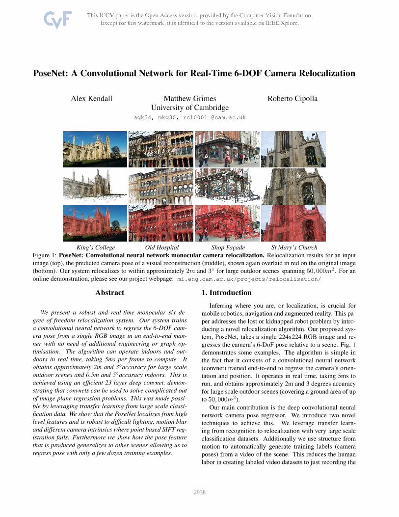
We found that training individual networks to regress

position and orientation separately performed poorly com-

pared to when they were trained with full 6-DOF pose la-

bels (fig. 2). With just position, or just orientation informa-

tion, the convnet was not as effectively able to determine the

function representing camera pose. We also experimented

with branching the network lower down into two separate

components to regress position and orientation. However,

we found that it too was less effective, for similar reasons:

separating into distinct position and orientation regressors

denies each the information necessary to factor out orienta-

tion from position, or vice versa.

In our loss function (2) a balance β must be struck be-

tween the orientation and translation penalties (fig. 2). They

are highly coupled as they are regressed from the same

model weights. We observed that the optimal β was given

by the ratio between expected error of position and orienta-

tion at the end of training, not the beginning. We found β

to be greater for outdoor scenes as position errors tended to

be relatively greater. Following this intuition we fine tuned

β using grid search. For the indoor scenes it was between

120 to 750 and outdoor scenes between 250 to 2000.

We found it was important to randomly initialize the fi-

nal position regressor layer so that the norm of the weights

corresponding to each position dimension was proportional

to that dimension’s spatial extent.

Classification problems have a training example for ev-

ery category. This is not possible for regression as the

Figure 2: Relative performance of position and orientation regres-

sion on a single convnet with a range of scale factors for an

indoor scene, Chess. This demonstrates that learning with the op-

timum scale factor leads to the convnet uncovering a more accurate

pose function.

output is continuous and infinite. Furthermore, other con-

vnets that have been used for regression operate off very

large datasets [25, 19]. For localization regression to work

off limited data we leverage the powerful representations

learned off these large classification datasets by pretraining

the weights on these datasets.

3.2. Architecture

For the experiments in this paper we use a state of

the art deep neural network architecture for classification,

GoogLeNet [24], as a basis for developing our pose regres-

sion network. GoogLeNet is a 22 layer convolutional net-

work with six ‘inception modules’ and two additional in-

termediate classifiers which are discarded at test time. Our

model is a slightly modified version of GoogLeNet with 23

layers (counting only the layers with trainable parameters).

We modified GoogLeNet as follows:

• Replace all three softmax classifiers with affine regres-

sors. The softmax layers were removed and each final

fully connected layer was modified to output a pose

vector of 7-dimensions representing position (3) and

orientation (4).

• Insert another fully connected layer before the final re-

gressor of feature size 2048. This was to form a local-

ization feature vector which may then be explored for

generalisation.

• At test time we also normalize the quaternion orienta-

tion vector to unit length.

We rescaled the input image so that the smallest dimension

was 256 pixels before cropping to the 224x224 pixel in-

put to the GoogLeNet convnet. The convnet was trained on

random crops (which do not affect the camera pose). At

test time we evaluate it with both a single center crop and

also densely with 128 uniformly spaced crops of the input

image, averaging the resulting pose vectors. With paral-

lel GPU processing, this results in a computational time in-

crease from 5ms to 95ms per image.

2940

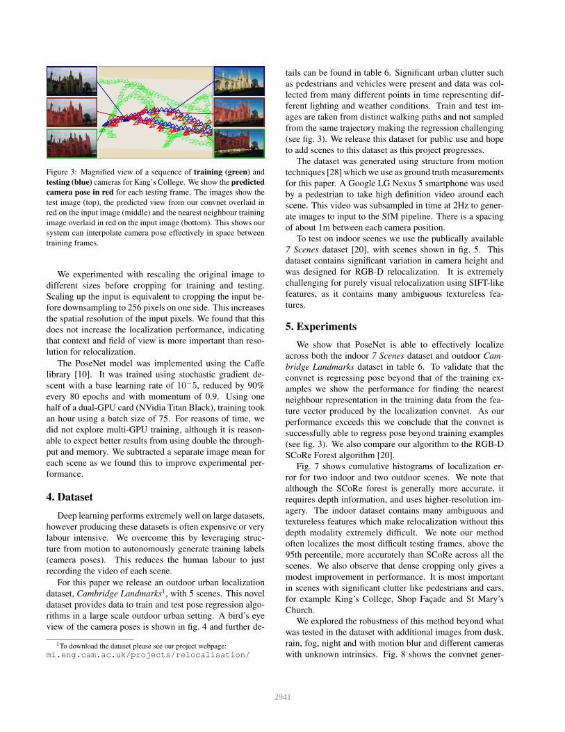
Figure 3: Magnified view of a sequence of training (green) and

testing (blue) cameras for King’s College. We show the predicted

camera pose in red for each testing frame. The images show the

test image (top), the predicted view from our convnet overlaid in

red on the input image (middle) and the nearest neighbour training

image overlaid in red on the input image (bottom). This shows our

system can interpolate camera pose effectively in space between

training frames.

We experimented with rescaling the original image to

different sizes before cropping for training and testing.

Scaling up the input is equivalent to cropping the input be-

fore downsampling to 256 pixels on one side. This increases

the spatial resolution of the input pixels. We found that this

does not increase the localization performance, indicating

that context and field of view is more important than reso-

lution for relocalization.

The PoseNet model was implemented using the Caffe

library [10]. It was trained using stochastic gradient de-

scent with a base learning rate of 10−5, reduced by 90%

every 80 epochs and with momentum of 0.9. Using one

half of a dual-GPU card (NVidia Titan Black), training took

an hour using a batch size of 75. For reasons of time, we

did not explore multi-GPU training, although it is reason-

able to expect better results from using double the through-

put and memory. We subtracted a separate image mean for

each scene as we found this to improve experimental per-

formance.

4. Dataset

Deep learning performs extremely well on large datasets,

however producing these datasets is often expensive or very

labour intensive. We overcome this by leveraging struc-

ture from motion to autonomously generate training labels

(camera poses). This reduces the human labour to just

recording the video of each scene.

For this paper we release an outdoor urban localization

dataset, Cambridge Landmarks1, with 5 scenes. This novel

dataset provides data to train and test pose regression algo-

rithms in a large scale outdoor urban setting. A bird’s eye

view of the camera poses is shown in fig. 4 and further de-

1To download the dataset please see our project webpage:

mi.eng.cam.ac.uk/projects/relocalisation/

tails can be found in table 6. Significant urban clutter such

as pedestrians and vehicles were present and data was col-

lected from many different points in time representing dif-

ferent lighting and weather conditions. Train and test im-

ages are taken from distinct walking paths and not sampled

from the same trajectory making the regression challenging

(see fig. 3). We release this dataset for public use and hope

to add scenes to this dataset as this project progresses.

The dataset was generated using structure from motion

techniques [28] which we use as ground truth measurements

for this paper. A Google LG Nexus 5 smartphone was used

by a pedestrian to take high definition video around each

scene. This video was subsampled in time at 2Hz to gener-

ate images to input to the SfM pipeline. There is a spacing

of about 1m between each camera position.

To test on indoor scenes we use the publically available

7 Scenes dataset [20], with scenes shown in fig. 5. This

dataset contains significant variation in camera height and

was designed for RGB-D relocalization. It is extremely

challenging for purely visual relocalization using SIFT-like

features, as it contains many ambiguous textureless fea-

tures.

5. Experiments

We show that PoseNet is able to effectively localize

across both the indoor 7 Scenes dataset and outdoor Cam-

bridge Landmarks dataset in table 6. To validate that the

convnet is regressing pose beyond that of the training ex-

amples we show the performance for finding the nearest

neighbour representation in the training data from the fea-

ture vector produced by the localization convnet. As our

performance exceeds this we conclude that the convnet is

successfully able to regress pose beyond training examples

(see fig. 3). We also compare our algorithm to the RGB-D

SCoRe Forest algorithm [20].

Fig. 7 shows cumulative histograms of localization er-

ror for two indoor and two outdoor scenes. We note that

although the SCoRe forest is generally more accurate, it

requires depth information, and uses higher-resolution im-

agery. The indoor dataset contains many ambiguous and

textureless features which make relocalization without this

depth modality extremely difficult. We note our method

often localizes the most difficult testing frames, above the

95th percentile, more accurately than SCoRe across all the

scenes. We also observe that dense cropping only gives a

modest improvement in performance. It is most important

in scenes with significant clutter like pedestrians and cars,

for example King’s College, Shop Facade and St Mary’s

Church.

We explored the robustness of this method beyond what

was tested in the dataset with additional images from dusk,

rain, fog, night and with motion blur and different cameras

with unknown intrinsics. Fig. 8 shows the convnet gener-

2941

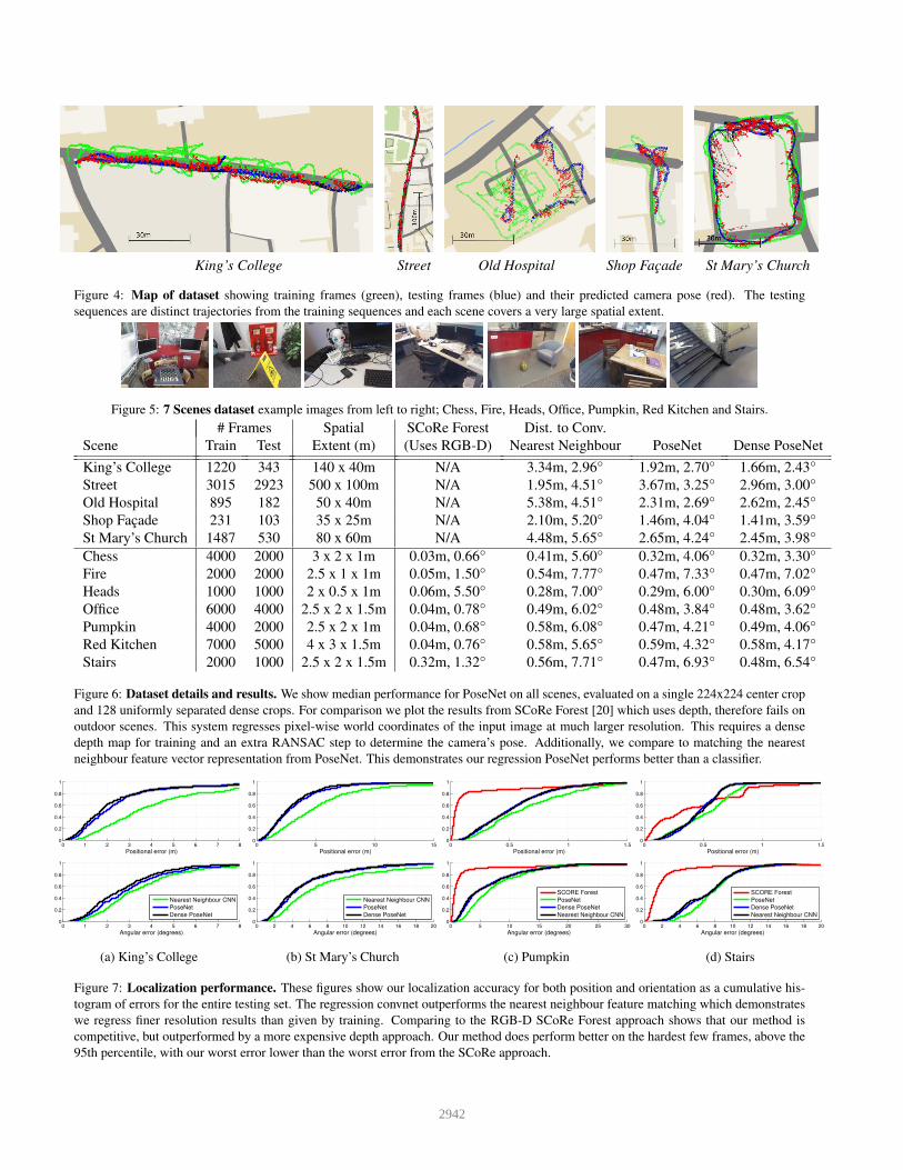
King’s College Street Old Hospital Shop Facade St Mary’s Church

Figure 4: Map of dataset showing training frames (green), testing frames (blue) and their predicted camera pose (red). The testing

sequences are distinct trajectories from the training sequences and each scene covers a very large spatial extent.

Figure 5: 7 Scenes dataset example images from left to right; Chess, Fire, Heads, Office, Pumpkin, Red Kitchen and Stairs.

# Frames Spatial SCoRe Forest Dist. to Conv.

Scene Train Test Extent (m) (Uses RGB-D) Nearest Neighbour PoseNet Dense PoseNet

King’s College 1220 343 140 x 40m N/A 3.34m, 2.96◦ 1.92m, 2.70◦ 1.66m, 2.43◦

Street 3015 2923 500 x 100m N/A 1.95m, 4.51◦ 3.67m, 3.25◦ 2.96m, 3.00◦

Old Hospital 895 182 50 x 40m N/A 5.38m, 4.51◦ 2.31m, 2.69◦ 2.62m, 2.45◦

Shop Facade 231 103 35 x 25m N/A 2.10m, 5.20◦ 1.46m, 4.04◦ 1.41m, 3.59◦

St Mary’s Church 1487 530 80 x 60m N/A 4.48m, 5.65◦ 2.65m, 4.24◦ 2.45m, 3.98◦

Chess 4000 2000 3 x 2 x 1m 0.03m, 0.66◦ 0.41m, 5.60◦ 0.32m, 4.06◦ 0.32m, 3.30◦

Fire 2000 2000 2.5 x 1 x 1m 0.05m, 1.50◦ 0.54m, 7.77◦ 0.47m, 7.33◦ 0.47m, 7.02◦

Heads 1000 1000 2 x 0.5 x 1m 0.06m, 5.50◦ 0.28m, 7.00◦ 0.29m, 6.00◦ 0.30m, 6.09◦

Office 6000 4000 2.5 x 2 x 1.5m 0.04m, 0.78◦ 0.49m, 6.02◦ 0.48m, 3.84◦ 0.48m, 3.62◦

Pumpkin 4000 2000 2.5 x 2 x 1m 0.04m, 0.68◦ 0.58m, 6.08◦ 0.47m, 4.21◦ 0.49m, 4.06◦

Red Kitchen 7000 5000 4 x 3 x 1.5m 0.04m, 0.76◦ 0.58m, 5.65◦ 0.59m, 4.32◦ 0.58m, 4.17◦

Stairs 2000 1000 2.5 x 2 x 1.5m 0.32m, 1.32◦ 0.56m, 7.71◦ 0.47m, 6.93◦ 0.48m, 6.54◦

Figure 6: Dataset details and results. We show median performance for PoseNet on all scenes, evaluated on a single 224x224 center crop

and 128 uniformly separated dense crops. For comparison we plot the results from SCoRe Forest [20] which uses depth, therefore fails on

outdoor scenes. This system regresses pixel-wise world coordinates of the input image at much larger resolution. This requires a dense

depth map for training and an extra RANSAC step to determine the camera’s pose. Additionally, we compare to matching the nearest

neighbour feature vector representation from PoseNet. This demonstrates our regression PoseNet performs better than a classifier.

0 1 2 3 4 5 6 7 80

0.2

0.4

0.6

0.8

1

Positional error (m)

0 1 2 3 4 5 6 7 80

0.2

0.4

0.6

0.8

1

Angular error (degrees)

Nearest Neighbour CNN

PoseNet

Dense PoseNet

(a) King’s College

0 5 10 150

0.2

0.4

0.6

0.8

1

Positional error (m)

0 2 4 6 8 10 12 14 16 18 200

0.2

0.4

0.6

0.8

1

Angular error (degrees)

Nearest Neighbour CNN

PoseNet

Dense PoseNet

(b) St Mary’s Church

0 0.5 1 1.50

0.2

0.4

0.6

0.8

1

Positional error (m)

0 5 10 15 20 25 300

0.2

0.4

0.6

0.8

1

Angular error (degrees)

SCORE Forest

PoseNet

Dense PoseNet

Nearest Neighbour CNN

(c) Pumpkin

0 0.5 1 1.50

0.2

0.4

0.6

0.8

1

Positional error (m)

0 2 4 6 8 10 12 14 16 18 200

0.2

0.4

0.6

0.8

1

Angular error (degrees)

SCORE Forest

PoseNet

Dense PoseNet

Nearest Neighbour CNN

(d) Stairs

Figure 7: Localization performance. These figures show our localization accuracy for both position and orientation as a cumulative his-

togram of errors for the entire testing set. The regression convnet outperforms the nearest neighbour feature matching which demonstrates

we regress finer resolution results than given by training. Comparing to the RGB-D SCoRe Forest approach shows that our method is

competitive, but outperformed by a more expensive depth approach. Our method does perform better on the hardest few frames, above the

95th percentile, with our worst error lower than the worst error from the SCoRe approach.

2942

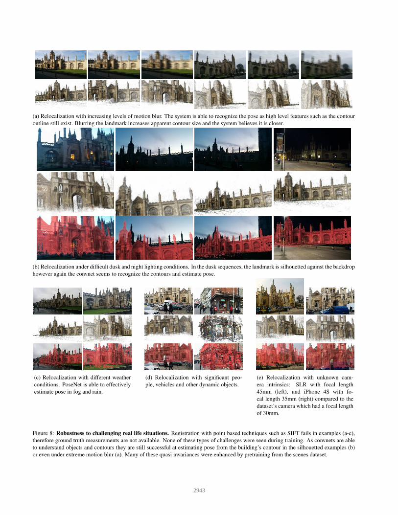
(a) Relocalization with increasing levels of motion blur. The system is able to recognize the pose as high level features such as the contour

outline still exist. Blurring the landmark increases apparent contour size and the system believes it is closer.

(b) Relocalization under difficult dusk and night lighting conditions. In the dusk sequences, the landmark is silhouetted against the backdrop

however again the convnet seems to recognize the contours and estimate pose.

(c) Relocalization with different weather

conditions. PoseNet is able to effectively

estimate pose in fog and rain.

(d) Relocalization with significant peo-

ple, vehicles and other dynamic objects.

(e) Relocalization with unknown cam-

era intrinsics: SLR with focal length

45mm (left), and iPhone 4S with fo-

cal length 35mm (right) compared to the

dataset’s camera which had a focal length

of 30mm.

Figure 8: Robustness to challenging real life situations. Registration with point based techniques such as SIFT fails in examples (a-c),

therefore ground truth measurements are not available. None of these types of challenges were seen during training. As convnets are able

to understand objects and contours they are still successful at estimating pose from the building’s contour in the silhouetted examples (b)

or even under extreme motion blur (a). Many of these quasi invariances were enhanced by pretraining from the scenes dataset.

2943

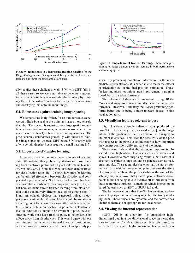
Figure 9: Robustness to a decreasing training baseline for the

King’s College scene. Our system exhibits graceful decline in per-

formance as fewer training samples are used.

ally handles these challenges well. SfM with SIFT fails in

all these cases so we were not able to generate a ground

truth camera pose, however we infer the accuracy by view-

ing the 3D reconstruction from the predicted camera pose,

and overlaying this onto the input image.

5.1. Robustness against training image spacing

We demonstrate in fig. 9 that, for an outdoor scale scene,

we gain little by spacing the training images more closely

than 4m. The system is robust to very large spatial separa-

tion between training images, achieving reasonable perfor-

mance even with only a few dozen training samples. The

pose accuracy deteriorates gracefully with increased train-

ing image spacing, whereas SIFT-based SfM sharply fails

after a certain threshold as it requires a small baseline [15].

5.2. Importance of transfer learning

In general convnets require large amounts of training

data. We sidestep this problem by starting our pose train-

ing from a network pretrained on giant datasets such as Im-

ageNet and Places. Similar to what has been demonstrated

for classification tasks, fig. 10 shows how transfer learning

can be utilised effectively between classification and com-

plicated regression tasks. Such ‘transfer learning’ has been

demonstrated elsewhere for training classifiers [18, 17, 2],

but here we demonstrate transfer learning from classifica-

tion to the qualitatively different task of pose regression. It

is not immediately obvious that a network trained to out-

put pose-invariant classification labels would be suitable as

a starting point for a pose regressor. We find, however, that

this is not a problem in practice. A possible explanation is

that, in order for its output to be invariant to pose, the clas-

sifier network must keep track of pose, to better factor its

effects away from identity cues. This would agree with our

own findings that a network trained to output position and

orientation outperforms a network trained to output only po-

0 20 40 60 80 100

Training epochs

Test err

or

AlexNet pretrained on PlacesGoogLeNet with random initialisationGoogLeNet pretrained on ImageNetGoogLeNet pretrained on PlacesGoogLeNet pretrained on Places, then another indoor landmark

Figure 10: Importance of transfer learning. Shows how pre-

training on large datasets gives an increase in both performance

and training speed.

sition. By preserving orientation information in the inter-

mediate representations, it is better able to factor the effects

of orientation out of the final position estimation. Trans-

fer learning gives not only a large improvement in training

speed, but also end performance.

The relevance of data is also important. In fig. 10 the

Places and ImageNet curves initially have the same per-

formance. However, ultimately the Places pretraining per-

forms better due to being a more relevant dataset to this

localization task.

5.3. Visualising features relevant to pose

Fig. 11 shows example saliency maps produced by

PoseNet. The saliency map, as used in [21], is the mag-

nitude of the gradient of the loss function with respect to

the pixel intensities. This uses the sensitivity of the pose

with respect to the pixels as an indicator of how important

the convnet considers different parts of the image.

These results show that the strongest response is ob-

served from higher-level features such as windows and

spires. However a more surprising result is that PoseNet is

also very sensitive to large textureless patches such as road,

grass and sky. These textureless patches may be more infor-

mative than the highest responding points because the effect

of a group of pixels on the pose variable is the sum of the

saliency map values over that group of pixels. This evidence

points to the net being able to localize off information from

these textureless surfaces, something which interest-point

based features such as SIFT or SURF fail to do.

The last observation is that PoseNet has an attenuated re-

sponse to people and other noisy objects, effectively mask-

ing them. These objects are dynamic, and the convnet has

identified them as not appropriate for localization.

5.4. Viewing the internal representation

t-SNE [26] is an algorithm for embedding high-

dimensional data in a low dimensional space, in a way that

tries to preserve Euclidean distances. It is often used, as

we do here, to visualize high-dimensional feature vectors in

2944

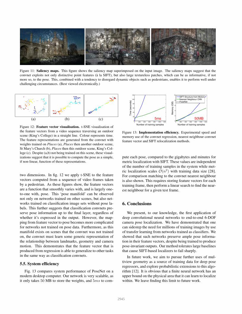
Figure 11: Saliency maps. This figure shows the saliency map superimposed on the input image. The saliency maps suggest that the

convnet exploits not only distinctive point features (a la SIFT), but also large textureless patches, which can be as informative, if not

more so, to the pose. This, combined with a tendency to disregard dynamic objects such as pedestrians, enables it to perform well under

challenging circumstances. (Best viewed electronically.)

(a) (b) (c)

Figure 12: Feature vector visualisation. t-SNE visualisation of

the feature vectors from a video sequence traversing an outdoor

scene (King’s College) in a straight line. Colour represents time.

The feature representations are generated from the convnet with

weights trained on Places (a), Places then another outdoor scene,

St Mary’s Church (b), Places then this outdoor scene, King’s Col-

lege (c). Despite (a,b) not being trained on this scene, these visual-

izations suggest that it is possible to compute the pose as a simple,

if non-linear, function of these representations.

two dimensions. In fig. 12 we apply t-SNE to the feature

vectors computed from a sequence of video frames taken

by a pedestrian. As these figures show, the feature vectors

are a function that smoothly varies with, and is largely one-

to-one with, pose. This ‘pose manifold’ can be observed

not only on networks trained on other scenes, but also net-

works trained on classification image sets without pose la-

bels. This further suggests that classification convnets pre-

serve pose information up to the final layer, regardless of

whether it’s expressed in the output. However, the map-

ping from feature vector to pose becomes more complicated

for networks not trained on pose data. Furthermore, as this

manifold exists on scenes that the convnet was not trained

on, the convnet must learn some generic representation of

the relationship between landmarks, geometry and camera

motion. This demonstrates that the feature vector that is

produced from regression is able to generalize to other tasks

in the same way as classification convnets.

5.5. System efficiency

Fig. 13 compares system performance of PoseNet on a

modern desktop computer. Our network is very scalable, as

it only takes 50 MB to store the weights, and 5ms to com-

0 200 400 600 800 1000 12000

20

40

60

80

100

120

Number of training samples

Tim

e (

seconds)

0 200 400 600 800 1000 12000

2

4

6

8

10

Number of training samples

Mem

ory

(G

B)

SIFT Structure from MotionNearest Neighbour CNNPoseNet

50MB5ms

Figure 13: Implementation efficiency. Experimental speed and

memory use of the convnet regression, nearest neighbour convnet

feature vector and SIFT relocalization methods.

pute each pose, compared to the gigabytes and minutes for

metric localization with SIFT. These values are independent

of the number of training samples in the system while met-

ric localization scales O(n2) with training data size [28].

For comparison matching to the convnet nearest neighbour

is also shown. This requires storing feature vectors for each

training frame, then perform a linear search to find the near-

est neighbour for a given test frame.

6. Conclusions

We present, to our knowledge, the first application of

deep convolutional neural networks to end-to-end 6-DOF

camera pose localization. We have demonstrated that one

can sidestep the need for millions of training images by use

of transfer learning from networks trained as classifiers. We

showed that such networks preserve ample pose informa-

tion in their feature vectors, despite being trained to produce

pose-invariant outputs. Our method tolerates large baselines

that cause SIFT-based localizers to fail sharply.

In future work, we aim to pursue further uses of mul-

tiview geometry as a source of training data for deep pose

regressors, and explore probabilistic extensions to this algo-

rithm [12]. It is obvious that a finite neural network has an

upper bound on the physical area that it can learn to localize

within. We leave finding this limit to future work.

2945

References

[1] S. Agarwal, Y. Furukawa, N. Snavely, I. Simon, B. Curless,

S. M. Seitz, and R. Szeliski. Building rome in a day. Com-

munications of the ACM, 54(10):105–112, 2011.

[2] Y. Bengio, A. Courville, and P. Vincent. Representa-

tion learning: A review and new perspectives. Pattern

Analysis and Machine Intelligence, IEEE Transactions on,

35(8):1798–1828, 2013.

[3] A. Bergamo, S. N. Sinha, and L. Torresani. Leveraging struc-

ture from motion to learn discriminative codebooks for scal-

able landmark classification. In Computer Vision and Pattern

Recognition (CVPR), 2013 IEEE Conference on, pages 763–

770. IEEE, 2013.

[4] M. Cummins and P. Newman. FAB-MAP: Probabilistic lo-

calization and mapping in the space of appearance. The

International Journal of Robotics Research, 27(6):647–665,

2008.

[5] J. Deng, W. Dong, R. Socher, L.-J. Li, K. Li, and L. Fei-

Fei. Imagenet: A large-scale hierarchical image database.

In Computer Vision and Pattern Recognition, 2009. CVPR

2009. IEEE Conference on, pages 248–255. IEEE, 2009.

[6] J. Donahue, Y. Jia, O. Vinyals, J. Hoffman, N. Zhang,

E. Tzeng, and T. Darrell. Decaf: A deep convolutional acti-

vation feature for generic visual recognition. arXiv preprint

arXiv:1310.1531, 2013.

[7] J. Engel, T. Schops, and D. Cremers. LSD-SLAM: Large-

scale direct monocular slam. In Computer Vision–ECCV

2014, pages 834–849. Springer, 2014.

[8] Y. Furukawa, B. Curless, S. M. Seitz, and R. Szeliski. To-

wards internet-scale multi-view stereo. In Computer Vision

and Pattern Recognition (CVPR), 2010 IEEE Conference on,

pages 1434–1441. IEEE, 2010.

[9] Q. Hao, R. Cai, Z. Li, L. Zhang, Y. Pang, and F. Wu. 3d

visual phrases for landmark recognition. In Computer Vision

and Pattern Recognition (CVPR), 2012 IEEE Conference on,

pages 3594–3601. IEEE, 2012.

[10] Y. Jia, E. Shelhamer, J. Donahue, S. Karayev, J. Long, R. Gir-

shick, S. Guadarrama, and T. Darrell. Caffe: Convolu-

tional architecture for fast feature embedding. arXiv preprint

arXiv:1408.5093, 2014.

[11] M. Kaess, H. Johannsson, R. Roberts, V. Ila, J. J. Leonard,

and F. Dellaert. iSAM2: Incremental smoothing and map-

ping using the bayes tree. The International Journal of

Robotics Research, page 0278364911430419, 2011.

[12] A. Kendall and R. Cipolla. Modelling uncertainty in

deep learning for camera relocalization. arXiv preprint

arXiv:1509.05909, 2015.

[13] G. Klein and D. Murray. Parallel tracking and mapping for

small ar workspaces. In Mixed and Augmented Reality, 2007.

ISMAR 2007. 6th IEEE and ACM International Symposium

on, pages 225–234. IEEE, 2007.

[14] Y. Li, N. Snavely, D. Huttenlocher, and P. Fua. Worldwide

pose estimation using 3d point clouds. In Computer Vision–

ECCV 2012, pages 15–29. Springer, 2012.

[15] D. G. Lowe. Distinctive image features from scale-

invariant keypoints. International journal of computer vi-

sion, 60(2):91–110, 2004.

[16] R. A. Newcombe, S. J. Lovegrove, and A. J. Davison.

DTAM: Dense tracking and mapping in real-time. In Com-

puter Vision (ICCV), 2011 IEEE International Conference

on, pages 2320–2327. IEEE, 2011.

[17] M. Oquab, L. Bottou, I. Laptev, and J. Sivic. Learning

and transferring mid-level image representations using con-

volutional neural networks. In Computer Vision and Pat-

tern Recognition (CVPR), 2014 IEEE Conference on, pages

1717–1724. IEEE, 2014.

[18] A. S. Razavian, H. Azizpour, J. Sullivan, and S. Carlsson.

Cnn features off-the-shelf: an astounding baseline for recog-

nition. In Computer Vision and Pattern Recognition Work-

shops (CVPRW), 2014 IEEE Conference on, pages 512–519.

IEEE, 2014.

[19] P. Sermanet, D. Eigen, X. Zhang, M. Mathieu, R. Fergus,

and Y. LeCun. Overfeat: Integrated recognition, localization

and detection using convolutional networks. arXiv preprint

arXiv:1312.6229, 2013.

[20] J. Shotton, B. Glocker, C. Zach, S. Izadi, A. Criminisi, and

A. Fitzgibbon. Scene coordinate regression forests for cam-

era relocalization in RGB-D images. In Computer Vision

and Pattern Recognition (CVPR), 2013 IEEE Conference on,

pages 2930–2937. IEEE, 2013.

[21] K. Simonyan, A. Vedaldi, and A. Zisserman. Deep inside

convolutional networks: Visualising image classification

models and saliency maps. arXiv preprint arXiv:1312.6034,

2013.

[22] N. Snavely, S. M. Seitz, and R. Szeliski. Photo tourism:

exploring photo collections in 3d. In ACM transactions on

graphics (TOG), volume 25, pages 835–846. ACM, 2006.

[23] N. Sunderhauf, F. Dayoub, S. Shirazi, B. Upcroft, and

M. Milford. On the performance of convnet features for

place recognition. arXiv preprint arXiv:1501.04158, 2015.

[24] C. Szegedy, W. Liu, Y. Jia, P. Sermanet, S. Reed,

D. Anguelov, D. Erhan, V. Vanhoucke, and A. Rabi-

novich. Going deeper with convolutions. arXiv preprint

arXiv:1409.4842, 2014.

[25] A. Toshev and C. Szegedy. Deeppose: Human pose estima-

tion via deep neural networks. In Computer Vision and Pat-

tern Recognition (CVPR), 2014 IEEE Conference on, pages

1653–1660. IEEE, 2014.

[26] L. Van der Maaten and G. Hinton. Visualizing data using

t-SNE. Journal of Machine Learning Research, 9(2579-

2605):85, 2008.

[27] J. Wang, H. Zha, and R. Cipolla. Coarse-to-fine vision-based

localization by indexing scale-invariant features. Systems,

Man, and Cybernetics, Part B: Cybernetics, IEEE Transac-

tions on, 36(2):413–422, 2006.

[28] C. Wu. Towards linear-time incremental structure from mo-

tion. In 3D Vision-3DV 2013, 2013 International Conference

on, pages 127–134. IEEE, 2013.

[29] B. Zhou, A. Lapedriza, J. Xiao, A. Torralba, and A. Oliva.

Learning deep features for scene recognition using places

database. In Advances in Neural Information Processing Sys-

tems, pages 487–495, 2014.

2946