arX

iv:a

stro

-ph/

9901

206v

1 1

5 Ja

n 19

99

Positron Escape from Type Ia Supernovae

P.A. Milne1 2

Naval Research Laboratory, Code 7650, Washington, DC 20375

L.-S. The, M.D. Leising

Department of Physics and Astronomy

Clemson,S.C., 29634-1911

Received ; accepted

1NAS/NRC Resident Research Associate.

2Much of this work was performed at Clemson University.

– 2 –

ABSTRACT

We generate bolometric light curves for a variety of type Ia supernova

models at late times, simulating gamma-ray and positron transport for various

assumptions about the magnetic field and ionization of the ejecta. These

calculated light curve shapes are compared with light curves of specific

supernovae for which there have been adequate late observations. From

these comparisons we draw two conclusions: whether a suggested model is

an acceptable approximation of a particular event, and, given that it is, the

magnetic field characteristics and degree of ionization that are most consistent

with the observed light curve shape. For the ten SNe included in this study,

five strongly suggest 56Co positron escape as would be permitted by a weak

or radially-combed magnetic field. Of the remaining five SNe, none clearly

show the upturned light curve expected for positron trapping in a strong,

tangled magnetic field. Chandrasekhar mass models can explain normally,

sub-, and super- luminous supernova light curves; sub-Chandrasekhar mass

models have difficulties with sub- (and potentially normally) luminous SNe. An

estimate of the galactic positron production rate from type Ia SNe is compared

with gamma-ray observations of Galactic 511 keV annihilation radiation.

Additionally, we emphasize the importance of correctly treating the positron

transport for calculations of spectra, or any properties, of type Ia SNe at late

epochs (≥ 200 d).

Subject headings: supernovae:general-gamma rays:observations,theory

– 3 –

1. INTRODUCTION

Many years of study of the light curves and spectra of type Ia supernovae have

revealed that a thermonuclear runaway induced by accretion on a white dwarf of ∼1 M⊙

(Hoyle & Fowler 1960) produces the energy to eject the entire star at ∼10,000 km s−1

and synthesizes ∼0.1-1.0 M⊙ of radioactive 56Ni. Prior to the maximum luminosity, the

ejecta are opaque and both the explosion energy and the energy from the 56Ni→56Co→56Fe

decays are deposited in and diffuse outward through the ejecta. After the bolometric light

curve reaches its peak, the luminosity approaches the instantaneous decay power (Arnett

1980; 1982) and the luminosity decline follows the decay of 56Co, with γ-ray scattering and

absorption dominating energy deposition. Later, due to expansion, γ-ray optical depth

decreases and the bolometric light curve decline becomes steeper than the 56Co decay.

Around t ≥ 200d, almost all γ-ray photons directly escape the ejecta and positrons from

the decay of 56Co provide the main source of energy deposition into the ejecta. At this

time, the light curve settles onto another, lower, 56Co decay curve. Beyond this time the

light curve evolution depends on the details of positron transport and energy loss. Here we

calculate energy deposition in type Ia supernovae (SNe Ia) for t ≥ 60d, when the photon

diffusion time is short and the bolometric luminosity is almost entirely due to gamma-ray

and positron energy loss processes.

There has been significant progress in understanding the physics of the early type

Ia light curves. Detailed radiation transport and expansion opacity computations have

reproduced observations of the bolometric and filter light curves (i.e., Pinto & Eastman

1998; Hoflich, Muller, & Khokhlov 1993; Woosley & Weaver 1986). It is clear that

the light curve’s rapid early evolution is due to the explosion of a low mass compact

object with a short radiative diffusion time (Arnett 1982; Pinto & Eastman 1998). The

secondary IR-maximum is the result of a photospheric radius that continues to expand

– 4 –

after visual maximum. The differences in pre-maximum rise-times among observed SNe

can be explained in model-dependent terms as due to the differences in a transition from

a deflagration flame to a detonation. The connections among peak luminosity, light curve

width, and post-maximum slope with the ejecta mass, 56Ni location, kinetic energy of

explosion, and opacity are explored in an elegant paper by Pinto & Eastman (1998).

Comparisons between early observed light curves and many various theoretical models have

been made extensively in recent years ( Hoflich, Wheeler, & Thielemann 1998; Hoflich et

al. 1996; Hoflich & Khokhlov 1996 (hereafter HK96)). We take the results of these works

as given and extend the comparison of the models and observations to later times.

For a few bright SNe Ia in the past half-century, good light curves beyond t ≥ 200d

have been obtained and studied. The first work that utilized the information from late

light curves was done by Colgate, Petschek, & Kriese (1980). They showed that the

late photographic and B band light curves of SN 1937C & SN 1972E can be explained

with positron kinetic energy deposition from 56Co decays, as suggested by Arnett (1969).

Recently Colgate (1991, 1997) analyzed late light curves with positron transport to infer

the ejecta mass. They found that ejecta somewhat transparent to positrons was required to

fit observed light curves. Cappellaro et al. (1997) (hereafter CAPP) studied the influence

of the mass of ejecta and the total mass of 56Ni on SN Ia light curves, and concluded that

the fraction of positron energy deposition varies among the five SNe Ia they analyzed, from

complete transparency to a complete trapping of the positrons. Ruiz-Lapuente & Spruit

(1998) (hereafter RLS) studied the effects of magnetic field geometry and magnitude in

exploding white dwarfs to explain observed SNe Ia bolometric light curves. They found

that the SN 1991bg magnetic field was weak (≤103G), while for SN 1972E a full trapping

of positrons by a tangled magnetic field in a Chandrasekhar mass model was required.

In addition to furthering our understanding of SNe Ia, we are motivated by the

– 5 –

possibility that the Galactic diffuse 511 keV emission might be due to the annihilation of

positrons that escape from SNe Ia, in addition to other possible sources such as core-collapse

SN radioactivity and compact objects. The long lifetime of energetic positrons in the ISM

(103-107 yrs) would mean that positrons from many SNe Ia would appear as a diffuse

component of the 511 keV line emission. Chan & Lingenfelter (1993) (hereafter CL)

calculated the number of surviving positrons from type Ia supernova models for different

magnetic field assumptions. Combining their positron yields with supernova rate estimates,

they suggested that type Ia SNe could provide from an insignificant to a dominant

contribution to the observed diffuse Galactic annihilation radiation flux – depending on the

magnetic field geometry. Average escape of a few per cent of 56Co positrons are necessary

to contribute to the Galactic emission, i.e., ≥50% of those emitted after one year would

have to escape. If the escapees take a significant fraction of their kinetic energy with them,

we might be able to see the power deficit in the measured light curves. Thus we hope to use

observed light curves to determine the SNe Ia contribution to Galactic positrons and obtain

information about the magnetic fields in SNe Ia.

Because of the variety of observed SN Ia properties and numerous physical details that

remain uncertain, there are many possible models allowed (for a review see Nomoto et al.

1996). We do not try to make judgements among them. We calculate the late bolometric

light curves of deflagration, delayed detonation, pulsed-delayed detonation, He detonation,

and accretion-induced collapse (AIC) models for comparison with observed light curves.

For each observed SN we consider the model(s) suggested by other authors to agree with

observations near maximum light. We begin by fitting each model to the observations

(to the inferred bolometric light curve when available) in the interval 100–200 days, when

gamma-ray energy deposition is still important. We then follow each model to later times

for various choices of magnetic field configuration and assumed ionization state of the

ejecta, and compare the calculated power deposited to the observed light curves.

– 6 –

In addition to the specific light curve consequences of positron transport we examine

some more generic features of the late light curves. We show that the light curve decline

rate between 60 and 200 days after the explosion can be used to clarify total ejecta mass

and expansion velocity of the supernova models. We find that the transition time between

the gamma-ray and positron dominated phases is a useful diagnostic to measure the ejecta

mass. In addition, the slope of the light curve at t ≥200 days is a good indicator of the

magnetic field configuration in the ejecta. As a baseline, we compare the calculated light

curves from positron transport with the light curve that results from the immediate, in-situ

kinetic energy deposition assumption, which has been typically assumed in early light curve

calculations.

The physics of energy deposition in type Ia SNe is discussed in section 2, followed by a

discussion of the strength and geometry of the magnetic field in the post-explosion ejecta.

Our bolometric light curves for both turbulent and radial field geometries are shown and

described in Section 3 for the various models used in our study. The issues confronting

fitting model generated light curves to actual observations are discussed in section 4. In

Section 5, we combine model predictions with SN data to fit a few of the best observed SNe.

We conclude with Section 6 in which we use positron yields from our models to estimate the

type Ia contribution to the observations of 511 keV annihilation radiation in the Galaxy.

2. Energy Deposition in SN Models

The 56Ni → 56Co (τ ∼ 8.8d) decay proceeds via electron capture (100%) and produces

photons and neutrinos. The line photons have energies between 0.16 and 1.56 MeV, with

a mean energy in photons of 1.75 MeV per decay. The 56Co → 56Fe (τ ∼ 111d) decay

proceeds 81% of the time via electron capture and 19% via positron emission (β+ decay).

The line photons have energies between 0.85 and 3.24 MeV, with mean energy in photons

– 7 –

per decay of 3.61 MeV. Segre (1977) derived the distribution of positron kinetic energy

(which is shown in figure 25). The mean positron kinetic energy is 0.63 MeV, so when

multiplied by the branching ratio 0.19, the mean positron energy per decay is 0.12 MeV.

The ratio of the mean photon energy to the mean positron kinetic energy is then ∼ 30. The

photon luminosity will dominate until the deposition fraction for positrons (fe+) is ∼ 30

times larger than the deposition fraction for photons (fγ). The energy deposition from both

gammas and positrons depend upon two factors; how much material must be traversed

enroute to the surface, and the interaction cross-sections. The transport of gamma rays and

positrons will be developed separately.

2.1. Gamma-Ray Transport

The gamma-line photons from the decays of 56Ni→56Co→56Fe are mostly Compton

scattered to lower energy during the early phases of the Type Ia event. These photons then

escape as X-ray continuum or are absorbed by material in the ejecta via the photo-electric

effect. Due to the supernova expansion, the gamma-line optical depth decreases, becoming

low enough at late-times that most gamma-line photons escape directly. In calculating

the energy deposition and the energy escape fraction of the photon energy created by the

radioactive decays, we simulate the scatter adopting the prescription of Podznyakov, Sobol,

& Sunyaev (1983). A detailed description of the Monte Carlo algorithm and its application

in calculating the spectra and bolometric light curves of SN1987A and type Ia supernovae

have been presented by The, Burrows, & Bussard (1990) and Burrows & The (1990).

Figure 1 shows the fraction of the total decay energy that escapes directly as

gamma-lines and emerges as X-ray continuum (fγ+X) as well as the fractions deposited

by scattering (fscat) and photoelectric absorption (fPE) as functions of time for model

W7 (Nomoto, Thielemann & Yokoi 1984), which we use for illustration here. The solid

– 8 –

curve labeled with fdep (= fscat + fPE) is the total gamma-ray energy deposition fraction.

Scattering dominates over photoelectric absorption at all times, the photoelectric absorption

becoming relatively less important as there become fewer multiply scattered photons at

late times. The overall photon deposition fractionscales roughly as t−2, reflecting the time

dependence of the column depth to the surface from any location in the ejecta.

2.2. Positron Transport

The cross sections for the various modes of positron annihilation are strongly

energy-dependent and favor low energies. Energetic positrons will move through the

ejecta until slowed to thermal velocities and then quickly annihilate.3 Five energy-loss

mechanisms were included: ionization and excitation of bound electrons, synchrotron

emission, bremsstrahlung emission, inverse Compton scattering, and plasma losses. The

first four are described in detail in CL. We include these processes in a calculation of model

W7, first assuming a uniformly 1% ionized medium (i.e., 0.01 free electrons per nucleus)

and then a uniformly triply ionized medium. The results, shown in figure 2, support CL’s

conclusion that for low ionization, the interactions with bound electrons dominate the

energy loss. For higher ionization, we find that plasma energy losses must be included.

Regardless of the ionization, processes other than ionization and excitation and plasma

losses can be ignored.

The ionization and excitation energy loss rate used is (Heitler 1954; Blumenthal &

Gould 1970; Gould 1972; Berger & Seltzer 1954),

3The lifetime of positrons once thermalized is small compared to the slowing time and to

the decay timescale, so for this study we set it equal to zero.

– 9 –

(

dE

dξ

)

ie

= −4πr2

omec2ZB

β2Amn

ln

√γ − 1γβ

Imec2

+1

2ln2

−β2

12

(

23

2+

7

γ + 1+

5

(γ + 1)2+

2

(γ + 1)3

)]

, (1)

where E is the positron’s kinetic energy, ro is the classical electron radius, and me and

mn are the electron and atomic mass unit masses respectively. ZB and A are the effective

nuclear charge and atomic mass of the ejecta. I is the effective ionization potential and is

approximated by Segre (1977) and by Roy & Reed(1968) as,

I = 9.1Z(

1 +1.9

Z2

3

)

eV. (2)

The plasma energy loss was described by Axelrod (1980). The formula is the same as

ionization and excitation, except hωp is inserted in the calculation of the maximum impact

parameter (bmax) rather than the mean ionization potential (I), and χe, the number of

free electrons per nucleus (hereafter ionization fraction) is used rather than ZB. Thus, (ZB

+ χe)·n = Z·n is the total electron density. Ignoring small differences in the relativistic

corrections, when the two energy losses are summed,

(

dE

dξ

)

Total

=

(

dE

dξ

)

ie

+

(

dE

dξ

)

P lasma

= −4πr2

omec2ZP (E)

β2Amn

[

Zln

(

√

γ − 1γβmec2

)

− ZBlnI − χeln(hωP )]

, (3)

where P(E) is the relativistic correction. There is an ionization fraction dependence due to

the inequality between lnI and ln(hωP ). An ionized medium is more efficient at slowing

positrons than is a neutral medium. The ionization fraction must be known as a function

– 10 –

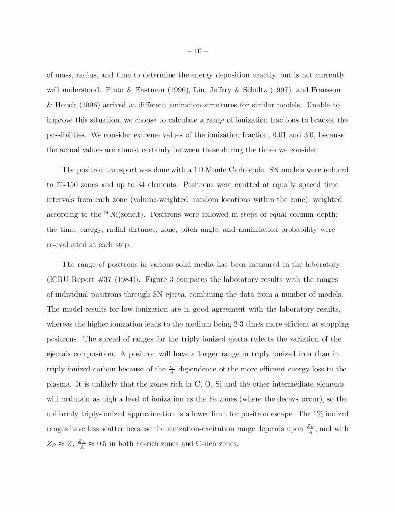
of mass, radius, and time to determine the energy deposition exactly, but is not currently

well understood. Pinto & Eastman (1996), Liu, Jeffery & Schultz (1997), and Fransson

& Houck (1996) arrived at different ionization structures for similar models. Unable to

improve this situation, we choose to calculate a range of ionization fractions to bracket the

possibilities. We consider extreme values of the ionization fraction, 0.01 and 3.0, because

the actual values are almost certainly between these during the times we consider.

The positron transport was done with a 1D Monte Carlo code. SN models were reduced

to 75-150 zones and up to 34 elements. Positrons were emitted at equally spaced time

intervals from each zone (volume-weighted, random locations within the zone), weighted

according to the 56Ni(zone,t). Positrons were followed in steps of equal column depth;

the time, energy, radial distance, zone, pitch angle, and annihilation probability were

re-evaluated at each step.

The range of positrons in various solid media has been measured in the laboratory

(ICRU Report #37 (1984)). Figure 3 compares the laboratory results with the ranges

of individual positrons through SN ejecta, combining the data from a number of models.

The model results for low ionization are in good agreement with the laboratory results,

whereas the higher ionization leads to the medium being 2-3 times more efficient at stopping

positrons. The spread of ranges for the triply ionized ejecta reflects the variation of the

ejecta’s composition. A positron will have a longer range in triply ionized iron than in

triply ionized carbon because of the χe

Adependence of the more efficient energy loss to the

plasma. It is unlikely that the zones rich in C, O, Si and the other intermediate elements

will maintain as high a level of ionization as the Fe zones (where the decays occur), so the

uniformly triply-ionized approximation is a lower limit for positron escape. The 1% ionized

ranges have less scatter because the ionization-excitation range depends upon ZB

A, and with

ZB ≈ Z, ZB

A≈ 0.5 in both Fe-rich zones and C-rich zones.

– 11 –

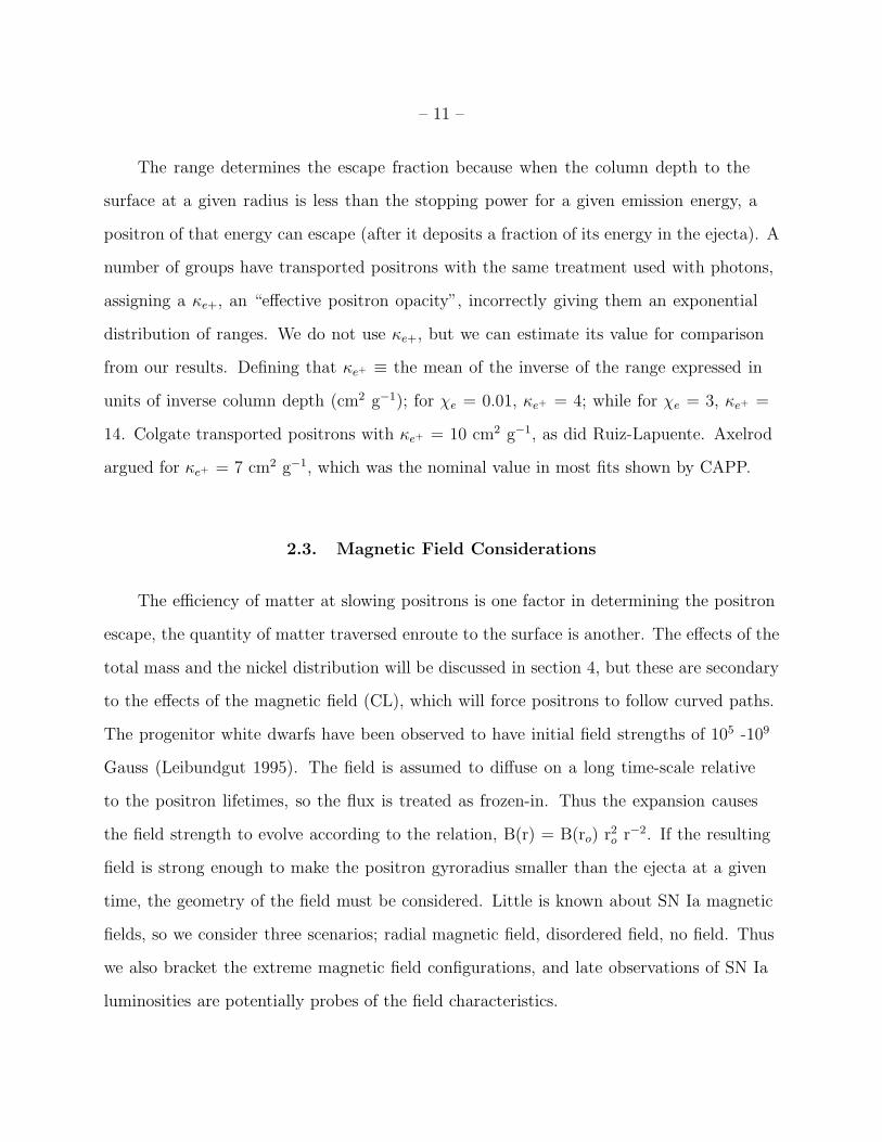
The range determines the escape fraction because when the column depth to the

surface at a given radius is less than the stopping power for a given emission energy, a

positron of that energy can escape (after it deposits a fraction of its energy in the ejecta). A

number of groups have transported positrons with the same treatment used with photons,

assigning a κe+, an “effective positron opacity”, incorrectly giving them an exponential

distribution of ranges. We do not use κe+, but we can estimate its value for comparison

from our results. Defining that κe+ ≡ the mean of the inverse of the range expressed in

units of inverse column depth (cm2 g−1); for χe = 0.01, κe+ = 4; while for χe = 3, κe+ =

14. Colgate transported positrons with κe+ = 10 cm2 g−1, as did Ruiz-Lapuente. Axelrod

argued for κe+ = 7 cm2 g−1, which was the nominal value in most fits shown by CAPP.

2.3. Magnetic Field Considerations

The efficiency of matter at slowing positrons is one factor in determining the positron

escape, the quantity of matter traversed enroute to the surface is another. The effects of the

total mass and the nickel distribution will be discussed in section 4, but these are secondary

to the effects of the magnetic field (CL), which will force positrons to follow curved paths.

The progenitor white dwarfs have been observed to have initial field strengths of 105 -109

Gauss (Leibundgut 1995). The field is assumed to diffuse on a long time-scale relative

to the positron lifetimes, so the flux is treated as frozen-in. Thus the expansion causes

the field strength to evolve according to the relation, B(r) = B(ro) r2o r−2. If the resulting

field is strong enough to make the positron gyroradius smaller than the ejecta at a given

time, the geometry of the field must be considered. Little is known about SN Ia magnetic

fields, so we consider three scenarios; radial magnetic field, disordered field, no field. Thus

we also bracket the extreme magnetic field configurations, and late observations of SN Ia

luminosities are potentially probes of the field characteristics.

– 12 –

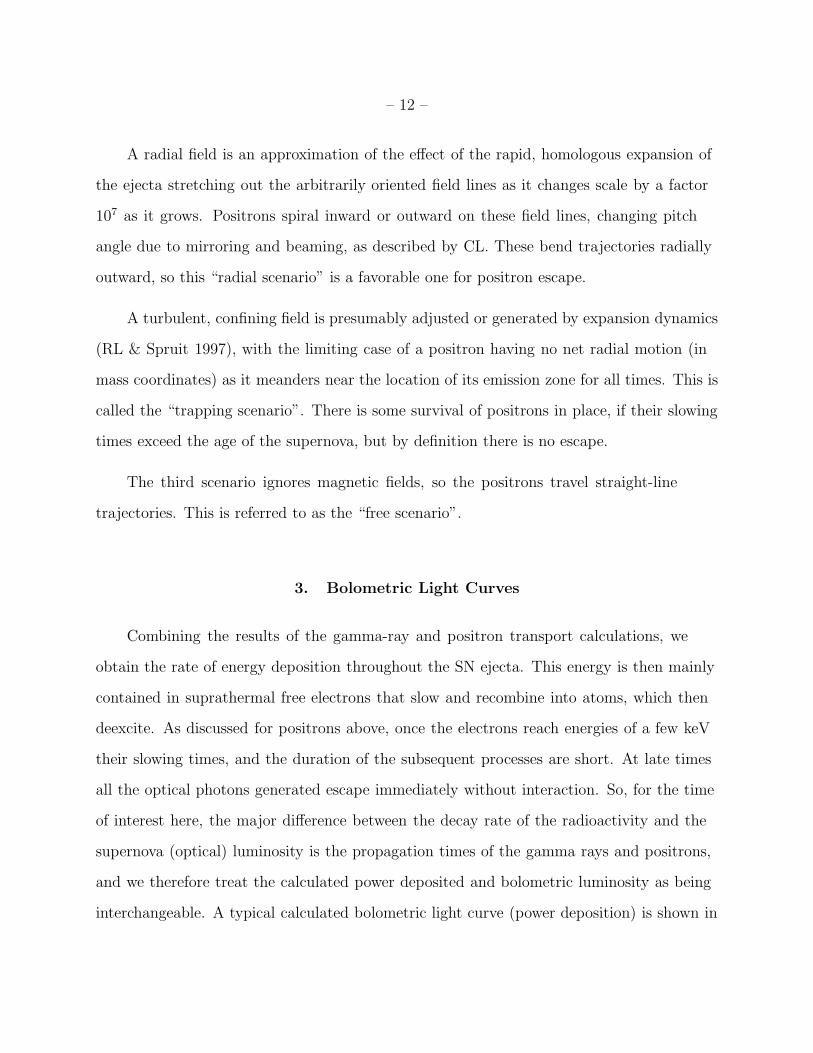
A radial field is an approximation of the effect of the rapid, homologous expansion of

the ejecta stretching out the arbitrarily oriented field lines as it changes scale by a factor

107 as it grows. Positrons spiral inward or outward on these field lines, changing pitch

angle due to mirroring and beaming, as described by CL. These bend trajectories radially

outward, so this “radial scenario” is a favorable one for positron escape.

A turbulent, confining field is presumably adjusted or generated by expansion dynamics

(RL & Spruit 1997), with the limiting case of a positron having no net radial motion (in

mass coordinates) as it meanders near the location of its emission zone for all times. This is

called the “trapping scenario”. There is some survival of positrons in place, if their slowing

times exceed the age of the supernova, but by definition there is no escape.

The third scenario ignores magnetic fields, so the positrons travel straight-line

trajectories. This is referred to as the “free scenario”.

3. Bolometric Light Curves

Combining the results of the gamma-ray and positron transport calculations, we

obtain the rate of energy deposition throughout the SN ejecta. This energy is then mainly

contained in suprathermal free electrons that slow and recombine into atoms, which then

deexcite. As discussed for positrons above, once the electrons reach energies of a few keV

their slowing times, and the duration of the subsequent processes are short. At late times

all the optical photons generated escape immediately without interaction. So, for the time

of interest here, the major difference between the decay rate of the radioactivity and the

supernova (optical) luminosity is the propagation times of the gamma rays and positrons,

and we therefore treat the calculated power deposited and bolometric luminosity as being

interchangeable. A typical calculated bolometric light curve (power deposition) is shown in

– 13 –

figure 4.

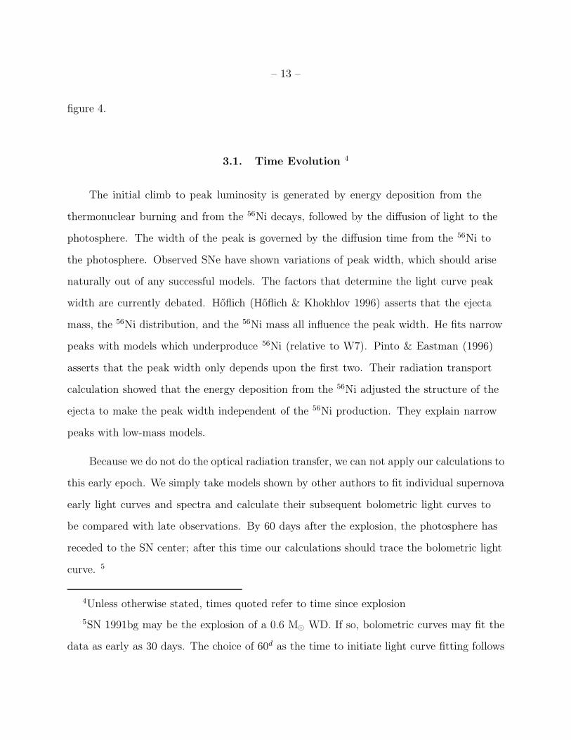
3.1. Time Evolution 4

The initial climb to peak luminosity is generated by energy deposition from the

thermonuclear burning and from the 56Ni decays, followed by the diffusion of light to the

photosphere. The width of the peak is governed by the diffusion time from the 56Ni to

the photosphere. Observed SNe have shown variations of peak width, which should arise

naturally out of any successful models. The factors that determine the light curve peak

width are currently debated. Hoflich (Hoflich & Khokhlov 1996) asserts that the ejecta

mass, the 56Ni distribution, and the 56Ni mass all influence the peak width. He fits narrow

peaks with models which underproduce 56Ni (relative to W7). Pinto & Eastman (1996)

asserts that the peak width only depends upon the first two. Their radiation transport

calculation showed that the energy deposition from the 56Ni adjusted the structure of the

ejecta to make the peak width independent of the 56Ni production. They explain narrow

peaks with low-mass models.

Because we do not do the optical radiation transfer, we can not apply our calculations to

this early epoch. We simply take models shown by other authors to fit individual supernova

early light curves and spectra and calculate their subsequent bolometric light curves to

be compared with late observations. By 60 days after the explosion, the photosphere has

receded to the SN center; after this time our calculations should trace the bolometric light

curve. 5

4Unless otherwise stated, times quoted refer to time since explosion

5SN 1991bg may be the explosion of a 0.6 M⊙ WD. If so, bolometric curves may fit the

data as early as 30 days. The choice of 60d as the time to initiate light curve fitting follows

– 14 –

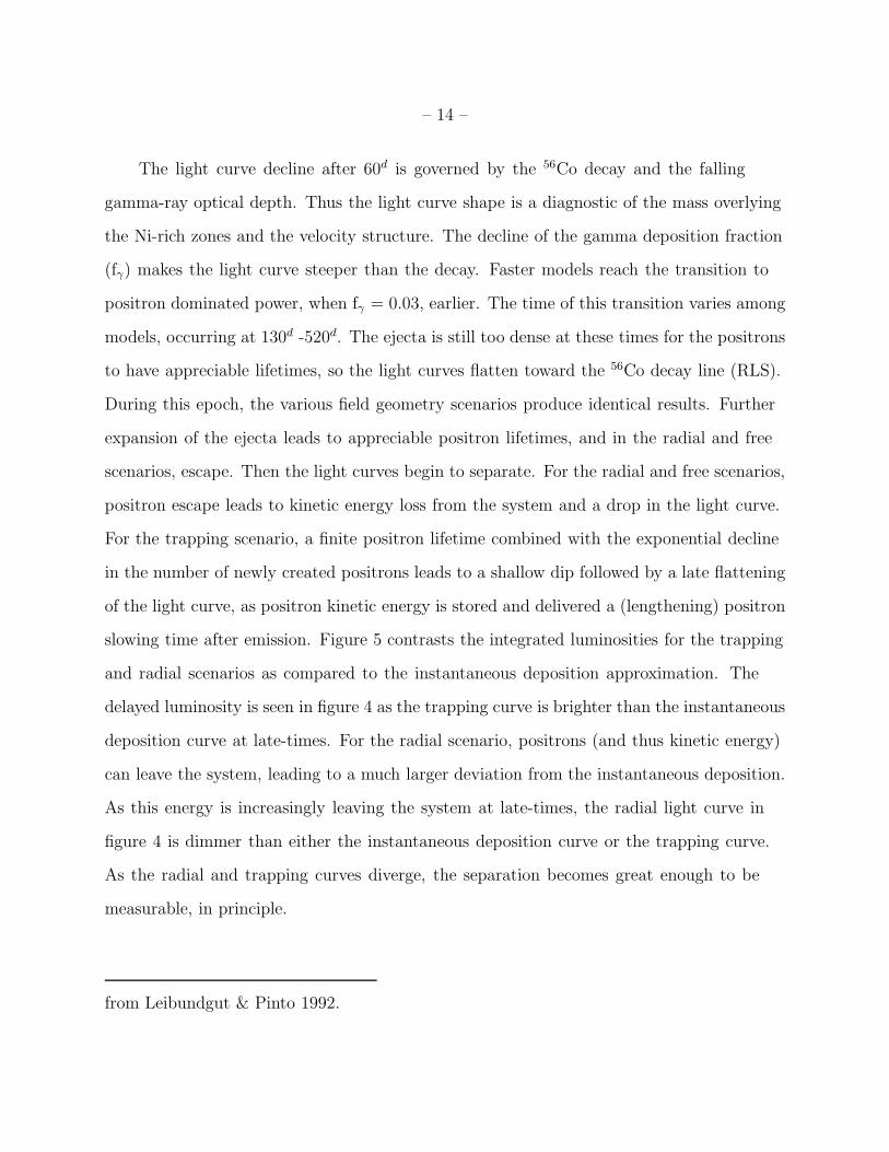
The light curve decline after 60d is governed by the 56Co decay and the falling

gamma-ray optical depth. Thus the light curve shape is a diagnostic of the mass overlying

the Ni-rich zones and the velocity structure. The decline of the gamma deposition fraction

(fγ) makes the light curve steeper than the decay. Faster models reach the transition to

positron dominated power, when fγ = 0.03, earlier. The time of this transition varies among

models, occurring at 130d -520d. The ejecta is still too dense at these times for the positrons

to have appreciable lifetimes, so the light curves flatten toward the 56Co decay line (RLS).

During this epoch, the various field geometry scenarios produce identical results. Further

expansion of the ejecta leads to appreciable positron lifetimes, and in the radial and free

scenarios, escape. Then the light curves begin to separate. For the radial and free scenarios,

positron escape leads to kinetic energy loss from the system and a drop in the light curve.

For the trapping scenario, a finite positron lifetime combined with the exponential decline

in the number of newly created positrons leads to a shallow dip followed by a late flattening

of the light curve, as positron kinetic energy is stored and delivered a (lengthening) positron

slowing time after emission. Figure 5 contrasts the integrated luminosities for the trapping

and radial scenarios as compared to the instantaneous deposition approximation. The

delayed luminosity is seen in figure 4 as the trapping curve is brighter than the instantaneous

deposition curve at late-times. For the radial scenario, positrons (and thus kinetic energy)

can leave the system, leading to a much larger deviation from the instantaneous deposition.

As this energy is increasingly leaving the system at late-times, the radial light curve in

figure 4 is dimmer than either the instantaneous deposition curve or the trapping curve.

As the radial and trapping curves diverge, the separation becomes great enough to be

measurable, in principle.

from Leibundgut & Pinto 1992.

– 15 –

3.2. Radial Magnetic Field vs No Field

It turns out that there is surprisingly little difference in the mean path traversed

to the surface for these two cases. Assuming isotropic emission of positrons, the mean

distance to the surface from a given point, for positrons not near the center of the ejecta,

is substantially larger than the radial distance to the surface because of the large solid

angle perpendicular to the radius. In the radial field case, mirroring and beaming turn

positron trajectories outward, but the extra path due to the spiral around the field adds

similar distance as in the no-field case. The net energy deposition and positron escape for

the models we consider are almost indistinguishable for these two cases. This result was

anticipated by Colgate (1996), and can be approximately demonstrated analytically. We

display radial field calculations, but remind the reader that for our spherically symmetric

models the conclusions apply equally to field-free scenarios. For a few of the models, there

were slight deviations at late-times (t ≥ 800d, the field-free curves remaining steeper than

the radial curves). We show field-free light curves only when the separation between these

these two cases is potentially detectable.

3.3. Energy Deposition at Very Late Times ( 1000d)

The effects of positron escape on the SN light curve are moderated somewhat by

gamma-ray energy deposition. Longer-lived radioactivities that were overwhelmed at earlier

epochs become important at late times. Two such radionuclei are 57Ni and 44Ti. The decay

of 57Ni proceeds with τNi57 = 52h and τCo57 = 392d, thus at 500d, 28% of the 57Co has yet

to decay. The 57Co decay energy is only 1/10 that of the 56Co. For W7 the energy available

from 57Co equals that available from 56Co at 1000d. Other models have similar 57Ni/56Ni

ratios. 44Ti is an even longer-liver radionucleus, with a mean-life recently estimated to be

85y± 1y (Ahmad et al. 1997). The 1.3 MeV decay energy is substantial, but the slow decay

– 16 –

rate delays the cross-over to 44Ti dominated deposition until 2500d, when no SN Ia has been

detected. Five models had the 57Co and 44Ti masses included. For the other models, MCo57

= 0.041 MCo56 and MT i44 = 1.5 x 10−5 MCo56, to match W7. Figure 6 shows the fraction

of the luminosity that is due to the deposition of positron KE. The positron deposition is

dominant from 300d -800d for the radial field geometry. The effects of including longer-lived

radioactivities is shown by the splitting of the curves at late times.

3.4. Additional Potential Sources and Effects

There are a number of other potential sources of luminosity, both intrinsic and

extrinsic. One extrinsic source is the “light echo”, bright peak light scattered by dust back

into the line of sight after light travel delays. SN 1991T was dominated by a light echo by

day 600 (Schmidt et al. 1994), as discussed in section 4. Another extrinsic source is the

interaction of the ejecta with the surrounding medium. This interaction will eventually be

important, but should be identified by distinctive spectral and temporal characteristics.

The SN model light curves presented in this work are based on the assumption that

the deposited power is instantly radiated in the UVOIR bands, during the time 1–2 years.

Furthermore, during this epoch, we usually have only the V and/or B band observations,

instead of the bolometric luminosity, with which to compare models. Fitting model light

curves to single or dual bands is susceptible to intrinsic spectral evolution effects. As

the secondary electrons’ lifetimes increase and the collisional de-excitation rates fall, a

delay develops between the positron energy deposition and emission of UVOIR light, an

effect called “freeze-out” by Fransson (1996). If the Fe I and II states form in abundance

without photoionization or charge exchange destruction, then [FeII]λ25.99µ, λ35.35µ, and

[FeI]λ24.05µ fine structure emission lines are produced. These lines are beyond the UBVRI

bands and are undetected. This effect is referred to as an infrared catastrophe (IRC) by

– 17 –

Axelrod (1980). Both freeze-out and IRC phenomena must be considered and are discussed

in section 5. It is clear that at very late times, many complicating effects, including new

sources of luminosity and sinks outside the normally observed bands can be important.

Therefore we confine our conclusions to the times when 56Co decay dominates the power

input and the B and V bands track well the bolometric luminosity.

3.5. SN Models

We considered twenty-one models, which span the range of ejecta mass, 56Ni mass, and

kinetic energy. One deflagration (W7) (Nomoto, Thielemann & Yokoi 1984), a normally

luminous helium detonation (HED8) (HK96), two subluminous helium detonations (WD065,

HED6) (Ruiz-Lapuente et al. 1993; HK96), two superluminous helium detonations (HECD,

HED9) (Kumagai 1997; HK96), one accretion-induced collapse (ONeMg) (Nomoto 1996),

eight delayed or late detonations (DD4, M36, M35, M39, DD2O2C, DD23c, W7DN, W7DT)

(Woosley 1991; Hoflich 1995; Hoflich, Wheeler & Thielemann 1998; Yamaoka 1992), three

pulsed, delayed detonations (PDD3, PDD54, PDD1b) (Hoflich, Khokhlov & Wheeler 1995),

and two mergers (DET2, DET2ENV6) were included. Their characteristics are shown in

Table 1.

In figure 7 we show the luminosity due only to the gamma deposition. As expected,

the total luminosity roughly traces the amount of 56Ni produced. The steepness of the

early decline measures the mass overlying the Ni. The models then flatten, with slopes

becoming nearly equal. In figure 8 we add the positron contribution to create bolometric

light curves for radial field geometries, assuming 1% ionization. The curves start at

and are normalized to 60d to show the evolution of their shape from 60d -400d. There

are often many observations during this epoch, so the different shapes provide a test of

whether the model (regardless of field characteristics) fits the light curve. One interesting

– 18 –

feature is the steepness of the Chandrasekhar mass models, in which the 56Ni is covered

by a large overlying mass. We interpret this steepness to be due to the delayed onset

of the positron-dominated epoch. The low mass models enter this epoch earlier, so they

flatten toward the decay line. Table 1 shows the day when gamma deposition falls to

equal the positron deposition. HED6, WD065, ONeMg, DET2 have relatively little mass

and transition before 180d; PDD1b and DET2ENV6 have much more overlying mass and

transition at 300d or later. PDD1b thins to gamma photons so slowly, that it remains as

bright as the low mass models due primarily to gamma deposition. Other than the extreme

model PDD1b, shallow declines after 60d suggest models with less mass overlying the 56Ni,

steep declines suggest more overlying mass. This trend is also evident in the light curves

calculated by RLS, who parametrize the slope at various epochs in their Table 3. The

separation of WD065 and ONeMg from HED6 after 200d is due to the earlier survival of

positrons in WD065 and ONeMg.

Figure 9 is an extension of figure 8 to 1000d, but including the curves from positron

trapping scenarios. This epoch emphasizes the differences in positron transport between the

field geometries. The most noticeable feature is that the radial models are approximately

equivalent and steep, whereas the trapping models flatten according to the percentage of

56Ni produced in the outer portions of the SN. RLS mention that the late light curves of

trapping field scenarios flatten relative to instantaneous deposition, but state that the effect

is small. Our results show the effect to be large. Thus, the 400d -800d, positron-dominated

epoch is a diagnostic of field characteristics, not of model types. Also apparent in this figure

is that the “massive” models show separation between the field scenarios much later and to

a lesser degree than the rest of the models. Massive in this sense refers to a large mass of

slow ejecta overlying the 56Ni-rich zones.

The variety of shapes at early epochs and then the dramatic separation between the

– 19 –

predictions of positron trapping in a turbulent field geometry and positron escape in a radial

or weak field show that 60d and later bolometric light curves yield a wealth of information

as to the structure and dynamics of the SN ejecta.

4. Comparison With Observed Light Curves

Ideally, to probe the SN structure using light curves, model-generated bolometric

light curves are compared with observed bolometric light curves. Observed bolometric

light curve reconstructions, to date, are at best based on measurements in the U,B,V,R,I

bands, with some information from the J,H and K bands. As the SN dims, the photometric

uncertainties increase and for many light curves, the number of bands observed decreases,

leading to less accurate bolometric reconstructions. We use the available bolometric light

curves: SN 1992A to day 420 (Suntzeff 1996), SN 1991bg to day 220 (Turratto et al. 1996),

SN 1972E to day 420 (Axelrod 1980) 6, SN 1989B to day 135, and SN 1991T to day 108

(Suntzeff 1996). The best epoch to observe positron transport effects is during the 500d

-900d range; only SN 92A and SN 72E extend close to that epoch. Nonetheless, the SN

91bg, SN 89B and SN 91T light curves are valuable in checking the fit of a specific model

during the gamma-dominated phase. For each model we consider for a particular event,

we simply fit the calculated light curve to the “observed” bolometric light curve. Thus we

avoid the uncertainties in distance, extinction, and bolometric correction. We then show

the later, positron-dominated light curves relative to this fit for comparison to the more

limited data in one or a few bands. RLS fit models to the bolometric luminosities of SN

1991bg and SN 1992A, Mazzali et al. (1996) fit SN 1991bg. In sections 5.1 5.2 and 5.4 we

6We do not use the 720 day data point because we consider the extrapolation of an entire

bolometric light curve from a 1200A wide spectrum to be too uncertain

– 20 –

will discuss our results in relation to theirs.

When there is insufficient data to reconstruct bolometric light curves we compare

model bolometric shapes to individual band photometry. This assumes that at late epochs

there is little color evolution. We must be able to rule out any increasing shift of the

luminosity into unobserved bands. Lira (1998) showed that the collective tendency is for

the color indices stop evolving after day 100-120d. In figure 10 we show the U, B, V, R,

and I band variations of six of the SNe used in this study. B-V peaks around t≃30-40d,

then decreases to approximately zero near day 100 (except SN 1991bg). At the (B-V)

peak, the V band contains most of the energy and then declines to B-V ≃ 0 with the B

band a potentially important contributor. The V band is the best single band to trace the

supernova bolometric light curve. The five bolometric light curves permit us to estimate the

error introduced by fitting with only the V band. As shown in figure 11, the inaccuracies in

using the V or B band data for the bolometric luminosity are ≤0.2m during the 60d-120d

epoch. The similar procedure in comparing model-generated bolometric light curves to

band photometry was also employed by CAPP who used V band data for every epoch.

Theoretical arguments about color evolution have been made by Axelrod and Colgate

(1996), who disagree as to whether collisional or radiative processes dominate the emission

from the recombination cascade. The competition between collisional and radiative

processes hinges upon three factors: level of ionization (temperature in the collisional

scenario), density, and atomic cross sections. Fransson & Houck (1996) addressed these

issues, calculating multi-band model light curves. The technique worked well for the type

II SN 1987A, but the type Ia light curves generated from the model DD4 showed a sharp

decrease in U,B,V,R,I around day 500 due to the infrared catastrophe (IRC), and were

inconsistent with SN 1972E. Why the IRC does not apparently occur in SN Ia is something

of a puzzle. The model DD3 contains more 56Ni (0.93 M⊙ versus 0.62 M⊙ for DD4) and

– 21 –

thus maintains a higher level of ionization. This delayed the onset of the IRC, but still

could not fit the observed light curves of SN 72E. It is important for our discussion that

any onset of the IRC is abrupt; this does not lead to a gentle decline of the light curve

as we find for positron escape. Fransson & Houck (1996) also considered clumping in the

ejecta. It might delay the onset of the IRC for the inter-clump regions, but it hastens its

onset in the clumps. It remains to be seen if spectra modeled with clumping will reproduce

the observed spectra.

The atomic cross sections provide a third explanation for the lack of color evolution.

If the radiative transition probabilities are underestimated, the radiative scenario might

dominate. Fransson & Houck increased the recombination rates by a factor of 3 to model

the spectra; perhaps additional adjustments are required. Few of the SNe observed at late

epochs show convincing color evolution. Two of the three SNe that continue to evolve after

120d, 1986G and 1994D, seem to settle into constant color indices later. All the evidence

suggests to us that the V (and probably B) band tracks the bolometric luminosity of SN Ia

at late times. We emphasize the SNe for which there are at least two measured bands for

most of the observed light curve.

5. Comparison of Models to Individual SNe

The amount, type, and quality of data varies among SNe. A summary of the

observations used in this study are listed in table 2. A wider range of model fits to SNe is

shown in Milne (1998). We primarily consider SN Ia models shown by others to describe

well the early light curves and/or spectra of particular well-observed events, calculating

their light curves to late times. Models are considered for a given event if they can

reproduce some combination of the following features: distance-dependent peak luminosity

estimates, rise-time to peak luminosity and peak width, early spectral features and light

– 22 –

curve shapes for multiple color bands. Generally the early data available do not uniquely

define the model parameters, or even the basic type of model. For some cases, the suggested

models are quite different. An example of this is SN 1991bg, which is fit with two low-mass

models (an 0.6 M⊙ AIC and a 0.65 M⊙ HeDET), a 1.4 M⊙ pulsed model and a 1.4 M⊙

deflagration model. Our first test is whether a model can fit the earlier nebular light curve,

which probes the transition from gamma to positron domination. We then examine whether

models that pass this first test can determine the magnetic field configuration and degree

of ionization. Thus, this study is able to add another constraint to the SN fitting puzzle, as

well as determining if positrons escape from SN ejecta.

5.1. SN 1992A in NGC 1380

SN 1992A occurred in the S0 galaxy NGC 1380 and was observed extensively. It is

often held up as an example of a normal SN Ia. Extinction appears to be minimal, making

SN 1992A an excellent candidate for photometric analysis. SN 1992A is one of three SNe

treated in both RLS and CAPP. We show the fits of three models to SN 1992A: DD23C,

M39 and HED8. DD23C was fit on the recommendation of Peter Hoflich (1998), and also

because Kirshner et al. (1992) fit the spectral data with a modified version of DD4, which

is similar to DD23C. RLS combined the distance estimates to NGC 1380 with Suntzeff’s

UVOIR bolometric estimation to suggest that the peak bolometric luminosity was between

42.65 and 43.00 dex. This suggests that a sub-luminous model might be required.7 M39

7A recent study by Suntzeff et al. 1998 suggests that NGC 1365 (treated to represent

the center of the Fornax cluster) may be a foreground galaxy in the cluster. If this is the

case, then SN 1992A may be only mildly sub-luminous, and at a distance in agreement with

Branch et al. 1997.

– 23 –

is a delayed detonation that has a peak bolometric luminosity of 43.06. We choose it as

a compromise between the delayed detonation scenario suggested by the spectra, and the

low luminosity suggested by distance estimates.8 CAPP listed the distance to NGC 1380 as

16.9 Mpc, with E(B-V) = 0.00m, and fit the data with a 1.0 M⊙ model which produced 0.4

M⊙ of 56Ni. We instead use the similar model HED8.

Figure 12 shows the fits of DD23C and HED8 to the bolometric light curves of SN

1992A. For this object the bolometric light curves are reconstructed to late enough times

that we can use them directly to study positron energy input. Assuming a 0.025 dex

uncertainty for each data point, DD23C provided the best fit, varying only the overall

amplitude, of the suggested models in the 55–420d epoch, fitting with 81% confidence for

the radial curve. The trapping version of that model was rejected at the 99.91% confidence

even when renormalized. The numerical results are shown in table 3 for 1% ionization,

triple ionization with a radial field geometry, and for 1% ionization with a trapping field.

The low mass model, HED8 did not fit above the 10−4 level for any scenario. RLS also fit a

0.96 M⊙ model to SN 1992A. Our results are consistent with theirs in that the models are

brighter than the data after 100 days. The CAPP fit for 7 ≤ κe+ ≤ 10 remained too bright

from 20d–320d, also in agreement with our results. The best fitting class of models were the

delayed detonation models; W7, DET2ENV6 and PDD54 were the only models other than

delayed detonation models to fit at better than the 20% confidence level.

We show the fits of two models to the V data, DD23C and M39, in figure 13. Both

models follow the falling luminosity better with positron escape than with trapping. Fitting

time-invariant ionization scenarios to the V data with the published uncertainties, none

of the models provided a fit better than χ2/DOF=18. The numerical fits to the V band

8We note that the B-V color of M39 is too red to fit 92A according to the model generated

light curves of Hoflich, even with zero extinction.

– 24 –

data (table 2) show that with the scatter in excess of the stated uncertainties, none of the

models provide statistically acceptable fits. In absolute terms, our goodness-of-fit statistics

are questionable, but the fits are better for radial scenarios for almost every model.9

The other delayed detonation models yielded fits similar to DD23C and M39 for the V

data, demonstrating that the observation of positron escape at late times is not strongly

model-dependent. The 928d point might herald the onset of another source of power.

Possibilities include other radioactivity, such as 22Na or 44Ti (but not 57Co, which is too

weak), recombination energy lagging earlier, higher ionization input (Clayton et al. 1992,

Fransson & Kozma 1993), and positrons encountering circumstellar material, as well as

others. In summary for SN 1992A: delayed detonations are the most promising model

types, all of which overproduce the late light V light curves without escape of positrons.

5.2. SN 1991bg in NGC 4374

SN 1991bg occurred in the galaxy NGC 4374 and is the best observed member of a class

of sub-luminous SNe that have a fast decline from peak luminosity. SN 1991bg appeared to

be very red at peak suggesting either significant extinction (∼ 0.7m), an intrinsically red

SN, or both. The fact that SN 1991bg and SN 1986G continued to show color evolution

after 120d suggests that they were intrinsically different than normal SN Ia. We fit SN

1991bg with three models that have been suggested to explain this SN; WD065, PDD54

and ONeMg, as well as a fourth model, W7. The models WD065 (a helium detonation) and

ONeMg (an accretion induced collapse) decline faster from peak luminosity relative to 1.4

M⊙ models because they have less overlying mass (but similar velocity structures) leading

9The model DET2ENV6 fits the late V band data well (but less so the bolometric data)

and may warrant further investigation.

– 25 –

to a lower optical thickness. Ruiz-Lapuente (1993) fit WD065 to the maximum and nebular

spectra, and later (RLS) to the bolometric light curve. PDD5 is a pulsed delayed-detonation

model that produces very little 56Ni, and maintains a lower level of ionization (relative

to W7 and normally luminous models) which decreases the free-free opacity and thus the

overall opacity. Hoflich (1996) fit PDD5 to B,V,R,and I band data out to 75d, suggesting

the distance to NGC 4374 to be 18 ± 5 Mpc with E(B-V)=0.25m. PDD5 is unavailable, so

we use the similar PDD54. W7 was included because it provides the best fit of all models,

it has not been suggested by other authors. The fits for the four models to the bolometric

data are shown in figure 14; fits to the V data is shown in figures 15 and 16. Present in the

B and V data is a disagreement after 140d between the data taken by Leibundgut et al.

(1993) and that taken by Turatto (1996), the Turatto data suggesting the SN was fainter.10

The bolometric light curve was calculated by Turatto et al. (1996) from the photometric

data, and strongly relied upon the B and V bands. No models were able to reproduce the

steep decline of the Turatto data. Placing 0.04 dex error bars on the bolometric data after

50d and ignoring the data after 140d, PDD54 provided the best overall fit at the 27% level.

WD065b fit below the 2% level, ONeMg below 10−5. Every model remains too bright to fit

the bolometric data out to 250d, with no model fitting above the 1% level.

The B and V band data shows the models WD065 and ONeMg to be bright from

140d–250d, too bright to fit either set of data. PDD54 and W7 were able to fit the

Leibundgut data within the uncertainties. RLS fit WD065 to the bolometric data, invoking

the weak-field scenario. For our calculated WD065 light curve, the weak-field scenario was

fainter than the radial scenario, but the light curve remained too bright to fit the data.

The dashed line shows the prediction for 100% transparency to positrons (zero deposition

10The third data set of Filippenko tends to confirm the measurements of Turatto, but do

not extend beyond 140d.

– 26 –

of positron kinetic energy). This line fits the data, but there is no physical justification for

this extreme scenario. Our results agree with the results of CAPP, who tried to fit a 0.7M⊙

model that produced 0.1M⊙ of 56Ni and determined that only zero positron deposition

(κe+=0 in their terminology) would approximate the data. For ONeMg, the slope of our

bolometric light curve agrees with Nomoto et al. (1996) from 60d–90d. It is the 120d–450d

epoch that excludes ONeMg as an acceptable model. Mazzali et al.(1996) tried to reproduce

the spectra of SN 1991bg with a 0.62 M⊙ version of W7, and as a by-product generated

a bolometric light curve out to 220d post-explosion. Their light curve assumed positron

trapping and was too bright to fit the data after 110d. They argued that this epoch is too

early to expect positron escape and suggested that there is unseen emission leading to an

erroneously low bolometric light curve. Our light curves for the low-mass models WD065b

and ONeMg have the same characteristics as theirs, and positron escape is insufficient to

explain the low luminosity in the 110d–220d epoch.

The inability to fit any model to the Turatto data tempted us to favor the trend

emerging from the Leibundgut data over the Turatto data. But, the light curve from SN

1992K forbids that action. SN 1992K has near peak spectral and photometric properties

similar to SN 1991bg, and the B and V data follows a SN 1991bg-like shape. The V data

extends out to ∼155d. The existence of a second example of this steep decline forces us

to conclude that there exists a sub-class of type Ia SNe for which we are unable to fit the

light curves with the models in our possession without invoking a larger extinction than

suggested. The flatness of low mass models during the positron-dominated phase suggests

that that class of models possess the opposite tendency from that required. The solution to

this problem remains unclear.

– 27 –

5.3. SN 1990N in NGC 4639

SN 1990N was unusual in that Co lines were detected earlier than existing models

predicted and the intermediate mass elements had higher velocities (Leibundgut 1991). The

near-maximum and post-maximum spectra were normal, suggesting normal models such as

W7 could explain them. The late detonation model, W7DN, was created to fit the early

spectra and transition to W7. This was accomplished by having a deflagration accelerate

into a detonation at Mr=1.20M⊙. Yamaoka (1992) discussed how the extra 56Ni modifies

the rise to peak light to fit SN 1990N. Hoflich (1996) fit DET2ENV2/4 and PDD3 to the

multi-band photometry of SN 1990N, for a distance to NGC 4639 of 20 ± 5 Mpc. The

multi-band coverage is very good, but a bolometric light curve has not been published.

There was an unfortunate gap in the light curve from 70d–200d, as the SN was too close to

the Sun for observations, hampering our ability to differentiate among model types.

Figure 17 shows the models W7DN and PDD3 fit to the B and V data. Both models

fit the 190d–300d data well and then show a steepening consistent with positron escape.

The normally luminous DD and PDD models provided similar fits, with all models giving

worse fits for positron trapping.

5.4. SN 1972E in NGC 5253

SN 1972E was not observed pre-maximum and thus the models are not well constrained.

We assume the explosion date to be JD2441420 (Axelrod 1980). The photometry out to

+169d is photoelectric, with later photometry derived from spectra (Kirshner & Oke 1975).

The bolometric light curve published by Axelrod was also generated by a model fit to the

Kirshner spectra. We fit three models to 72E: W7, M35 and HED8. RLS fit W7 to the

bolometric data, invoking a transition from turbulent confinement (with Bo=105Ga) to

– 28 –

weak-field trajectories around 500d Their W7 light curve fit well before 500d. The transition

was discussed conceptually by RLS, but not modelled. Hoflich (1996) fit the model M35 to

the multi-band photometry of 72E, suggesting the distance NGC 5253 to be 4.0 ± 0.6 Mpc.

The model HED8 is shown because of the agreement with the bolometric light curve. All

three models are consistent with the 56Ni mass suggested by the nebular spectra, 0.5–0.6M⊙

(Ruiz-Lapuente & Lucy 1992). Colgate (1996) suggests a 0.4 M⊙ model to explain 72E,

this possibility was not investigated due to the lack of a suitable model.

Figure 18 shows the fits of HED8, W7, and M35 to the B, V and bolometric data.

None of these models can be rejected, but all fit better with the radial field scenario and

significant positron escape. None of the models fit the 700+d data point, with all remaining

too bright.

5.5. SN 1991T in NGC 4527

SN 1991T was unusual in the width of the luminosity peak and in the absence of SiII

and CaII absorption lines (Filippenko et al. 1997). It is the prototype of superluminous

type Ia SNe. It was also an example of a SN whose late emission was overwhelmed by a

light echo, as shown by Schmidt et al. (1994). Suntzeff (1996) derived a bolometric light

curve to 87d post-B maximum against which we tested models. There was also a gap in

observations as the sun was too near the SN. We show the fits of two models to SN 1991T,

the late-detonation W7DT, and the superluminous helium detonation HECD. The model

W7DT was proposed by Yamaoka et al. (1992) to explain the lack of intermediate mass

elements in the pre-maximum spectra, followed by a normal spectrum post-maximum.

Nomoto et al. (1996) modelled the bolometric light curve for W7DT and scaled it to fit the

V data. Hoflich (1996) suggested PDD3 and DET2ENV2 based upon fits to multi-band

photometry, suggesting the distance to NGC 4527 to be 12 ± 2 Mpc. Liu et al. (1997)

– 29 –

argued that the superluminous 1.1 M⊙ helium detonation, SC1.1 (which produces 0.8 M⊙ of

56Ni), fit the nebular spectrum (301d) better than did the models W7, DD4 and SC0.9. To

fit SN 1991T, Liu et al. (1997) assumed a distance of 12–14 Mpc and E(B-V)=0.0m–0.1m.

We approximate SC1.1 with HECD, a 1.06 M⊙ helium detonation that produces 0.72 M⊙

of 56Ni. Pinto & Eastmann (1996) fit DD4 (with pop. II elements added) to the B and V

data for SN 1991T out to 60d, suggesting a distance of 14 Mpc for E(B-V)=0.1m.

RLF estimated the 56Ni production to be 0.7–0.8 M⊙ of 56Ni using nebular spectra;

Bowers’ (1997) 56Ni production (when adjusted as explained in section 4) is 0.7±0.2 M⊙.

W7DT and HECD are both consistent with this, while PDD3 slightly underproduces 56Ni.

Figure 19 shows the fits of W7DT and HECD to the V data. The late V data was

fit by adding a constant light echo component. Both models show that the radial field

scenario with positron escape provides better fits. The dashed lines show the radial light

curves without an echo, the dot-dashed lines show the trapping light curves without an

echo. The trapping curves remain too bright during the 200d–500d epoch even with no

contribution from a light echo, arguing strongly against trapping. The 1.1 M⊙ and 1.4 M⊙

models have similar late light curves, suggesting that they can not resolve the ambiguity

between Chandrasekhar and sub-Chandrasekhar mass models for superluminous SNe. The

fact that the radial curve explains the data with no echo contribution until 470d perhaps

suggests that the light echo that “turned on” after 450d, an effect that could be explained

by the SN light sweeping through a dust cloud. The asymmetry of the image of the SN

1991T light echo would be consistent with reflection off of discrete cloud(s) (Boffi et al.

1998). Unfortunately, the light echo interrupted the positron dominated epoch before the

optimal time to observe positron escape (∼600d). Whereas it may be possible to eventually

account for and subtract out the contributions from a light echo, we do not fit light curves

into the light echo phase other than to demonstrate the phenomenon.

– 30 –

5.6. SN 1993L in IC 5270

SN 1993L was observed by CAPP and fit by the same model used for SN 1992A.

The strength of the SN 1993L data is the continuous multi-band photometry extending

to beyond 500d. The data were published without uncertainties. There are no published

spectra, so the best model was selected entirely by the fit to the B and V data. An

additional complication is that the SN was discovered after maximum, which eliminated

that discriminant. CAPP assumed the explosion date to be JD 2449098, the distance to

be 20.1 Mpc and the extinction to be E(B-V)=0.75m. With these assumptions, SN 1993L

appears to be quite similar to SN 1992A. CAPP noted two differences between the two

SNe; SN 1993L had a slower nebular velocity and a higher degree of V band curvature from

100d–500d. We note the additional difference that the SN 1993L light curve was dimmer

from 25d–55d and again from 100d to the cross-over at 400d. Explaining these features is

difficult, but we note that some of the PDD and DD models studied by Hoflich & Khokhlov

show these features.

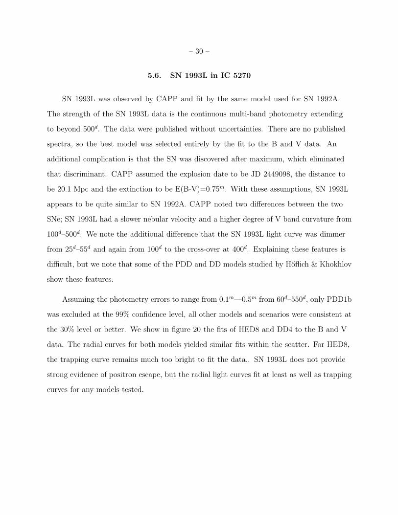
Assuming the photometry errors to range from 0.1m—0.5m from 60d–550d, only PDD1b

was excluded at the 99% confidence level, all other models and scenarios were consistent at

the 30% level or better. We show in figure 20 the fits of HED8 and DD4 to the B and V

data. The radial curves for both models yielded similar fits within the scatter. For HED8,

the trapping curve remains much too bright to fit the data.. SN 1993L does not provide

strong evidence of positron escape, but the radial light curves fit at least as well as trapping

curves for any models tested.

– 31 –

5.7. SN 1937C in IC 4182

SN 1937C reached a peak B magnitude of 8.71m and was detected on photographic

plates for over 600d. Branch, Romanishin & Baron (1996) have argued that that its spectral

features are those of normal SNe Ia, while Pierce & Jacoby (1995) argued that SN 1937C is

similar to SN 1991T and thus superluminous. Hoflich (HK96) suggests N32, W7 and DET2

as acceptable models, and a distance of 4.5 ± 1 Mpc. We use the data of Schaefer (1994),

which is a re-analysis of photographic plates from many observers, principally Baade (1938)

and Baade & Zwicky (1938). Pierce and Jacoby (1995) also re-analyzed photographic plates

of SN 1937C obtaining a higher value for Bmax=8.94m.

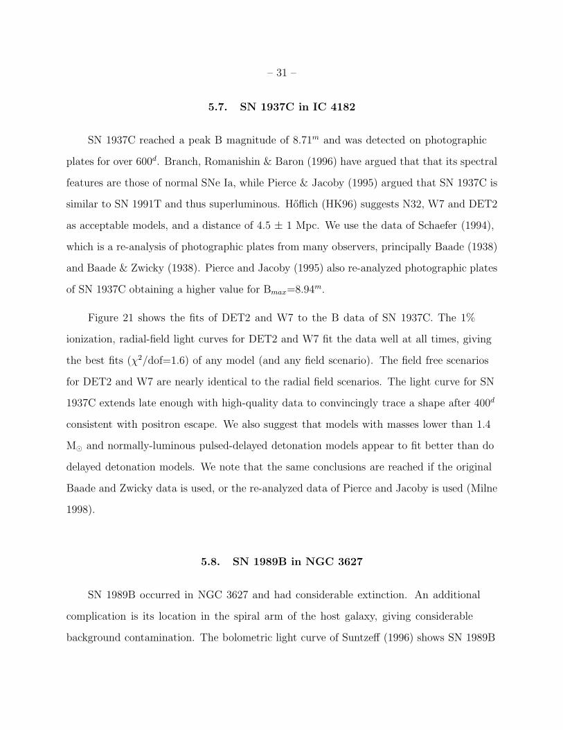
Figure 21 shows the fits of DET2 and W7 to the B data of SN 1937C. The 1%

ionization, radial-field light curves for DET2 and W7 fit the data well at all times, giving

the best fits (χ2/dof=1.6) of any model (and any field scenario). The field free scenarios

for DET2 and W7 are nearly identical to the radial field scenarios. The light curve for SN

1937C extends late enough with high-quality data to convincingly trace a shape after 400d

consistent with positron escape. We also suggest that models with masses lower than 1.4

M⊙ and normally-luminous pulsed-delayed detonation models appear to fit better than do

delayed detonation models. We note that the same conclusions are reached if the original

Baade and Zwicky data is used, or the re-analyzed data of Pierce and Jacoby is used (Milne

1998).

5.8. SN 1989B in NGC 3627

SN 1989B occurred in NGC 3627 and had considerable extinction. An additional

complication is its location in the spiral arm of the host galaxy, giving considerable

background contamination. The bolometric light curve of Suntzeff (1996) shows SN 1989B

– 32 –

to be similar to SN 1992A, but remaining brighter than SN 1992A from 90 days onward.

HK96 suggested the models M37 and M36 based upon fits to the multi-band photometry;

we fit M36 to B,V and bolometric data for SN 1989B. The distance suggested by HK96 is

8.7±3 Mpc.

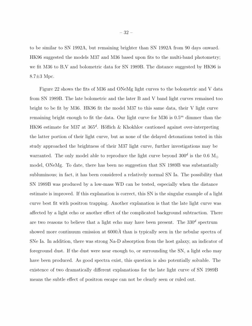
Figure 22 shows the fits of M36 and ONeMg light curves to the bolometric and V data

from SN 1989B. The late bolometric and the later B and V band light curves remained too

bright to be fit by M36. HK96 fit the model M37 to this same data, their V light curve

remaining bright enough to fit the data. Our light curve for M36 is 0.5m dimmer than the

HK96 estimate for M37 at 365d. Hoflich & Khokhlov cautioned against over-interpreting

the latter portion of their light curve, but as none of the delayed detonations tested in this

study approached the brightness of their M37 light curve, further investigations may be

warranted. The only model able to reproduce the light curve beyond 300d is the 0.6 M⊙

model, ONeMg. To date, there has been no suggestion that SN 1989B was substantially

subluminous; in fact, it has been considered a relatively normal SN Ia. The possibility that

SN 1989B was produced by a low-mass WD can be tested, especially when the distance

estimate is improved. If this explanation is correct, this SN is the singular example of a light

curve best fit with positron trapping. Another explanation is that the late light curve was

affected by a light echo or another effect of the complicated background subtraction. There

are two reasons to believe that a light echo may have been present. The 330d spectrum

showed more continuum emission at 6000A than is typically seen in the nebular spectra of

SNe Ia. In addition, there was strong Na-D absorption from the host galaxy, an indicator of

foreground dust. If the dust were near enough to, or surrounding the SN, a light echo may

have been produced. As good spectra exist, this question is also potentially solvable. The

existence of two dramatically different explanations for the late light curve of SN 1989B

means the subtle effect of positron escape can not be clearly seen or ruled out.

– 33 –

5.9. SN 1986G in NGC 5128

SN 1986G was well observed, but occurred in the dust lane of NGC 5128 and suffered

from considerable extinction. SN 1986G had a narrow peak and slow λ6355A Si lines,

suggesting that it was intermediate between normal SNe Ia and SN 1991bg. The B-V color

index continued to evolve 120d after the explosion, a feature also seen in SN 1991bg, but not

observed in normal SN Ia.11 We fit the models W7, M39 and HED6 to SN 1986G. HK96 fit

W7 to multi-band light curves to 80d post-explosion, suggesting the distance to NGC 5128

to be 4.2±1.2 Mpc. M39 was used because the 56Ni mass of M39 is in closer agreement with

the RLF estimate of 0.38±0.03M⊙. HED6 represents moderately sub-luminous, low-mass

models.

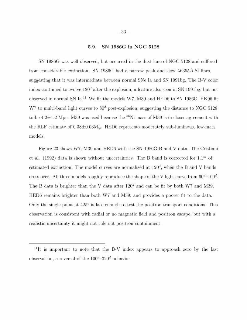
Figure 23 shows W7, M39 and HED6 with the SN 1986G B and V data. The Cristiani

et al. (1992) data is shown without uncertainties. The B band is corrected for 1.1m of

estimated extinction. The model curves are normalized at 120d, when the B and V bands

cross over. All three models roughly reproduce the shape of the V light curve from 60d–100d.

The B data is brighter than the V data after 120d and can be fit by both W7 and M39.

HED6 remains brighter than both W7 and M39, and provides a poorer fit to the data.

Only the single point at 425d is late enough to test the positron transport conditions. This

observation is consistent with radial or no magnetic field and positron escape, but with a

realistic uncertainty it might not rule out positron containment.

11It is important to note that the B-V index appears to approach zero by the last

observation, a reversal of the 100d–320d behavior.

– 34 –

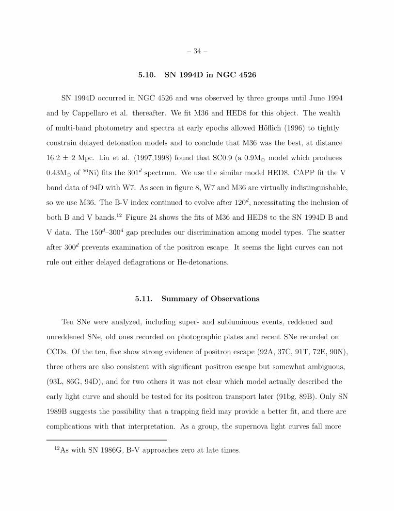
5.10. SN 1994D in NGC 4526

SN 1994D occurred in NGC 4526 and was observed by three groups until June 1994

and by Cappellaro et al. thereafter. We fit M36 and HED8 for this object. The wealth

of multi-band photometry and spectra at early epochs allowed Hoflich (1996) to tightly

constrain delayed detonation models and to conclude that M36 was the best, at distance

16.2 ± 2 Mpc. Liu et al. (1997,1998) found that SC0.9 (a 0.9M⊙ model which produces

0.43M⊙ of 56Ni) fits the 301d spectrum. We use the similar model HED8. CAPP fit the V

band data of 94D with W7. As seen in figure 8, W7 and M36 are virtually indistinguishable,

so we use M36. The B-V index continued to evolve after 120d, necessitating the inclusion of

both B and V bands.12 Figure 24 shows the fits of M36 and HED8 to the SN 1994D B and

V data. The 150d–300d gap precludes our discrimination among model types. The scatter

after 300d prevents examination of the positron escape. It seems the light curves can not

rule out either delayed deflagrations or He-detonations.

5.11. Summary of Observations

Ten SNe were analyzed, including super- and subluminous events, reddened and

unreddened SNe, old ones recorded on photographic plates and recent SNe recorded on

CCDs. Of the ten, five show strong evidence of positron escape (92A, 37C, 91T, 72E, 90N),

three others are also consistent with significant positron escape but somewhat ambiguous,

(93L, 86G, 94D), and for two others it was not clear which model actually described the

early light curve and should be tested for its positron transport later (91bg, 89B). Only SN

1989B suggests the possibility that a trapping field may provide a better fit, and there are

complications with that interpretation. As a group, the supernova light curves fall more

12As with SN 1986G, B-V approaches zero at late times.

– 35 –

quickly than models, which fit well at early times, extrapolated to later times with all the

positron kinetic energy deposited in and radiated by the ejecta. This is consistent with the

escape of a substantial fraction of the positrons emitted by 56Co after one year.

Regarding even earlier times, for sub-luminous SNe the Chandrasekhar mass models

fit the light curves better than low-mass models. For normally luminous SNe, there

are not enough observations from 60d–400d to choose between the model masses. The

superluminous SNe can apparently be fit equally well by high-mass He-detonation models

and nickel-rich Chandrasekhar mass models.

6. Type Ia SN Contributions to the Galactic 511 keV Emission

Table 3 shows the positron survival fraction of type Ia SNe at 2000d and the resulting

positron yields for all the models treated in this study. The range of values reflects the

extremes of ionization fractions. The lower values correspond to triple ionization, the

higher values are for 1% ionization. The yields vary between the two extremes by roughly

a factor of three. The observations suggest that 1% ionization typically fits better, so we

will quote 2/3 of that yield as a conservative estimate for each model. For radial fields, the

Chandrasehkar mass models have a lower survival fraction when compared with equally

luminous sub-Chandrasehkar mass models, but the larger nickel mass partially compensates

for that fact. As a result, for all but the “heavy ” models, the yields are not strongly

dependent upon model mass. The radial scenarios have greatly enhanced positron escape

yields compared to the trapping scenarios.

Positron escape is best observed best in light curves when its relative effect is large,

between 400d & 1000d, but the positron yield in absolute terms is determined earlier: 80%

of the escaping positrons do so between 178d -546d for W7 (94d -492d for HED8). It is

– 36 –

conceivable, but probably not common, that the trapping field could apply until, say, 500d,

when the field magnitude decreased to the point that the Larmor radius reached the ejecta

radius and the object would cross over to the field-free regime. The “release time” for a

positron of a given energy is proportional to the initial field strength, which might vary over

many orders of magnitude. For one object we might incorrectly infer the positron escape

for this reason, but not likely for many.

The positrons that escape retain a significant fraction of their emitted energy, as shown

by CL and in figure 25, which compares the emission spectrum (dashed line) to the escape

spectrum (solid line). With energies near 400 keV, the positrons have a considerable lifetime

in the ISM, giving diffuse galactic 511 keV emission. To estimate the rate of positron

injection into the ISM, we assume a 2:2:1 ratio of normal:subluminous:superluminous

SNe. Considering DD23C, PDD3, and HED8, a reasonable yield for normal SNe is 8 x

1052 positrons. For subluminous SNe, PDD54, DET2ENV6 suggest a yield of 4 x 1052

positrons. From W7DT, DD4, and HECD (suggested by 91T) we estimate a yield of 15 x

1052 positrons. Employing the above ratio then gives a mean yield of 8 x 1052 positrons per

SN Ia.

This gives a flux (4π D2)−1 · y · SNR · fe+γ, where D is the distance, y is the positron

yield per SN event, and SNR is the SN Ia rate, and fe+γ is the 511 keV photons emitted

per positron. Taking D=8 kpc, y=8 x 1052 e+ SN−1, SNR=0.0032 SN yr−113, and fPs=0.58

photons e+−1 (which corresponds to a positronium fraction of 0.95), the flux is 6.3 x

10−4 photons cm−2 s−1. An estimate of the uncertainty in this flux can be obtained by

inserting D=7.7 -8.5 kpc, y=3 -10 e+ SN−1, SNR=0.003 -0.06 SN yr−1, and fγe+−1=0.5

-0.65 (corresponding to a positronium fraction of 1.0 -0.9) into the formula. The flux then

13This value was obtained from Capellaro et al. (1997) and assumes Ho=65 km s−1 Mpc−1.

Hamuy & Pinto (1998) suggest a slightly larger value, 0.0042 SN yr−1.

– 37 –

ranges from (1.2 -8.6) x 10−4 photons cm−2 s−1. The flux is on the order of the Galactic

bulge component of the 511 keV flux as measured by OSSE. Purcell (1997) estimated the

bulge flux to be 3.5 x 10−4 photons cm−2 s−1 and the galactic plane flux to be 8.9 x 10−4

photons cm−2 s−1. SMM, with a 130◦ FOV, (Share et al. 1988) measured the total flux

from the general direction of the galactic center to be 2.4 x 10−3 photons cm−2 s−1; the type

Ia SN contribution could be one-fourth of that flux. A more exact treatment of the level of

agreement between the 511 keV flux as mapped by OSSE and the spatial distribution of Ia

SNe is the subject of a forthcoming paper (Milne 1999).

7. Summary

We calculate the γ-ray and the positron kinetic energy deposition to produce

“UBVOIR” bolometric light curves for the time when the photon diffusion time (t≥60d) is

short for various models of type Ia SNe. In calculating positron kinetic energy deposition

into the ejecta, we calculate it for particular extreme environments, they are: radial

magnetic field, turbulence magnetic field, and field free geometries in a 1% and triple

ionization medium throughout the evolution. The deposited energy rate is assumed to

instantaneously appear as “UBVOIR” bolometric luminosity and is compared with several

observed bolometric luminosity when they are available or with B and V bands observed

luminosity. In this work, we analyzed ten late time type Ia supernova light curves by

comparing the light curves with the calculated light curves. It can be shown clearly, that

all of the light curves except of SN 1991bg (explain below) require positron kinetic energy

deposition in order to give a reasonable agreement. Without the energy deposition, it is

quite obvious that the light curve is too dim to explain the observe light curve at t≥200d

(Colgate, Petschek, Kreise 1980; Capellaro et al. 1997; Ruiz-Lapuenta & Spruit 1997).

We show γ-ray energy deposition at t≥60d can hardly be used to distinguished light

– 38 –

curve shape between various models, except to differentiate between extreme models such as

between low (PDD1b) and high explosion energy models or between low sub-Chandrasekhar

mass (i.e. ONeMg) and Chandrasekhar mass (i.e. W7) models. A similar situation

also ensues in the epoch when positron kinetic energy deposition is dominant and for

the case of magnetic field in the ejecta being radially combed outward. In the case of

turbulence magnetic field, the usefulness of the late time light curve to differentiate models

is moderately improved due to the effectiveness of ejecta to slow down and to absorb the

kinetic energy of positrons.

The light curves of SN Ia are dominantly powered by the kinetic energy deposition

from β+ decay of positrons after the nebula becomes optically thin to gamma photons.

Before and at the onset of this “positron phase” the positrons have short lifetimes regardless

of the field geometry, but as the nebula becomes more tenuous positrons can survive

and possibly escape for favorable geometries. The longer the positrons stay as energetic

particles, the larger is the deficit of energy deposition relative to the full instantaneous

energy deposition. This effect is also observed when there are more positrons escape

from the ejecta. Comparing late time light curves of suggested models from early light

curve and spectra for particular observed supernovae, the deficit of luminosity relative

to instantaneous deposition can be seen in the B and/or the V band light curves of SNe

1992A, 1990N, 1937C, 1972E, 1991T. The phenomena give the evidence that positron take

its time in depositing its kinetic energy and possibly moves quite far from its origin and

even escapes from the ejecta.

Further detail comparisons of the calculated light curves of positron energy deposition

in radial and tangled magnetic field configurations of type Ia models with the observed

V and B band light curves show that the radial field configuration (or synonymously the

weak field configuration) produces a better agreement than does the tangled magnetic field

– 39 –

configuration, which produces light curves far too flat. The agreement that requires radial

field configuration is exhibited by the observed light curves of SN 1992A, SN 1937C, SN

1990N, SN 1972E, and SN 1991T. Models with tangled magnetic field configuration produce

a flatter and brighter light curves than the radial field configuration due to the more energy

deposition. There are a number of potential sources which can flatten the curves further,

but steepening the curves such as by IRC is difficult without color evolution, which to date

has not been observed in SN Ia light curve. These facts strengthen the argument that

positron escape occurs in SN Ia ejecta.

Fitting observed light curves of SN 1993L, SN 1994D, and SN 1986G give ambiguous

results that it is not clear which of the radial or the tangled magnetic configuration model

can give acceptable fit. The ambiguity is mostly due to the fluctuation in the observed B

and V band light curves. The strongest indication for the tangled magnetic configuration

seems to be shown by the SN 1989B observed light curve, however there is a possibility that

there is a contribution from a light echo at late times.

SN 1991bg is somewhat a special case that not all SN 1991bg observed light curves

agree with each other completely. Two light curves (Turatto et al. 1996; Filippenko et al.

1992) agree with each other, but no model that we have can give a reasonable fit to the

light curves unless we unphysically impose no positron kinetic energy deposition in the

ejecta. The light curve observed by Leibundgut et al. (1993) can be fit reasonably well with

model PDD54 and W7, but we cannot determine the magnetic field configuration in the

ejecta because of no observation done by Leibundgut et al. (1993) beyond day 200.

Based on the shape of SN 1937C, SN 1972E, and SN 1992A’s light curves, which all

follow the predictions of the radial field configuration model, we conclude that in these

supernovae the positrons escape with the most efficient transparency as if the positrons

moved in a straight line from their origins to the surface and deposit a minimum of their

– 40 –

kinetic energy as they escape. These supernovae show that type Ia SNe can be a dominant

source of the diffuse Galactic 511 keV line fluxes.

To better quantify the suggestion that type Ia supernova may be the main source of

positrons that produce the observed Galactic 511 keV line fluxes. We present the number

or fraction of positrons that escape from Ia models. The values are in agreement with the

values calculated by CL, who demonstrated that the radial magnetic field scenario can

easily provide the needed positrons to explain the Galactic annihilation line fluxes.

The Galactic 511 keV annihilation line flux distribution has a definite bulge component

(Purcell et al. 1997). SN Ia positrons from 56Co decays may contribute the majority of

the bulge flux and a sizable fraction of the entire galactic emission. As the number of SN

Ia observed in spiral galaxies increase, the spatial distribution of bulge and disk SNe will

be better known. As OSSE maps the galactic center region with increasing exposure and

spectral information, the level to which SN Ia positrons escape from SNe may soon be

known.

This work is from a dissertation which was submitted to the graduate school of

Clemson University by P.A.M. in partial fulfillment of the requirements for the PhD degree

in physics. P.A.M. would like to thank P. Ruiz-Lapuente for access to models and for

emphasizing the use of bolometric data when available. We thank P. Hoflich for access

to many models, giving assistance in locating data and for suggestions of models to test

against individual SNe. The isotopically complete models provided by K. Nomoto and S.

Kumagai were important for many additional applications. P.A.M. thanks D. Jeffery for

spectroscopic insight and assistance locating data. We thank P. Pinto for providing us

with model DD4 and for useful discussion on ionization fraction and plasma energy loss.

This work was supported by NASA grant DPR S-10987C, via sub-contract to Clemson

University.

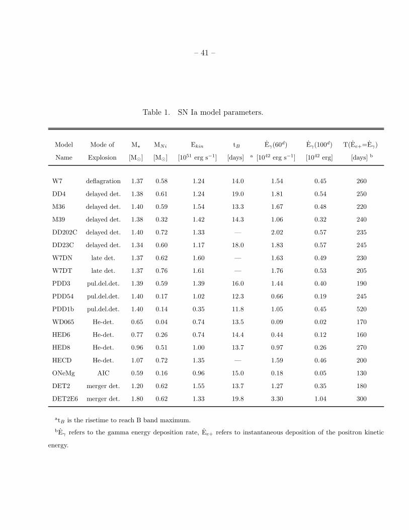
– 41 –

Table 1. SN Ia model parameters.

Model Mode of M⋆ MNi Ekin tB Eγ(60d) Eγ(100d) T(Ee+=Eγ)

Name Explosion [M⊙] [M⊙] [1051 erg s−1] [days] a [1042 erg s−1] [1042 erg] [days] b

W7 deflagration 1.37 0.58 1.24 14.0 1.54 0.45 260

DD4 delayed det. 1.38 0.61 1.24 19.0 1.81 0.54 250

M36 delayed det. 1.40 0.59 1.54 13.3 1.67 0.48 220

M39 delayed det. 1.38 0.32 1.42 14.3 1.06 0.32 240

DD202C delayed det. 1.40 0.72 1.33 — 2.02 0.57 235

DD23C delayed det. 1.34 0.60 1.17 18.0 1.83 0.57 245

W7DN late det. 1.37 0.62 1.60 — 1.63 0.49 230

W7DT late det. 1.37 0.76 1.61 — 1.76 0.53 205

PDD3 pul.del.det. 1.39 0.59 1.39 16.0 1.44 0.40 190

PDD54 pul.del.det. 1.40 0.17 1.02 12.3 0.66 0.19 245

PDD1b pul.del.det. 1.40 0.14 0.35 11.8 1.05 0.45 520

WD065 He-det. 0.65 0.04 0.74 13.5 0.09 0.02 170

HED6 He-det. 0.77 0.26 0.74 14.4 0.44 0.12 160

HED8 He-det. 0.96 0.51 1.00 13.7 0.97 0.26 270

HECD He-det. 1.07 0.72 1.35 — 1.59 0.46 200

ONeMg AIC 0.59 0.16 0.96 15.0 0.18 0.05 130

DET2 merger det. 1.20 0.62 1.55 13.7 1.27 0.35 180

DET2E6 merger det. 1.80 0.62 1.33 19.8 3.30 1.04 300

atB is the risetime to reach B band maximum.

bEγ refers to the gamma energy deposition rate, Ee+ refers to instantaneous deposition of the positron kinetic

energy.

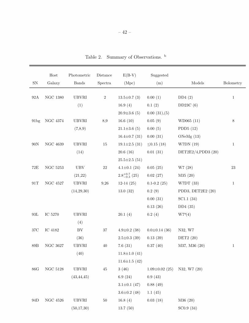
– 42 –

Table 2. Summary of Observations. b

Host Photometric Distance E(B-V) Suggested

SN Galaxy Bands Spectra (Mpc) (m) Models Bolometry

92A NGC 1380 UBVRI 2 13.5±0.7 (3) 0.00 (1) DD4 (2) 1

(1) 16.9 (4) 0.1 (2) DD23C (6)

20.9±3.6 (5) 0.00 (31),(5)

91bg NGC 4374 UBVRI 8,9 16.6 (10) 0.05 (9) WD065 (11) 8

(7,8,9) 21.1±3.6 (5) 0.00 (5) PDD5 (12)

16.4±0.7 (31) 0.00 (31) ONeMg (13)

90N NGC 4639 UBVRI 15 19.1±2.5 (31) ≤0.15 (18) W7DN (19) 1

(14) 20.6 (16) 0.01 (31) DET2E2/4,PDD3 (20)

25.5±2.5 (51)

72E NGC 5253 UBV 22 4.1±0.1 (24) 0.05 (25) W7 (28) 23

(21,22) 2.8+0.7−0.3 (25) 0.02 (27) M35 (20)

91T NGC 4527 UBVRI 9,26 12-14 (25) 0.1-0.2 (25) W7DT (33) 1

(14,29,30) 13.0 (32) 0.2 (9) PDD3, DET2E2 (20)

0.00 (31) SC1.1 (34)

0.13 (26) DD4 (35)

93L IC 5270 UBVRI 20.1 (4) 0.2 (4) W7a(4)

(4)

37C IC 4182 BV 37 4.9±0.2 (38) 0.0±0.14 (36) N32, W7

(36) 2.5±0.3 (39) 0.13 (39) DET2 (20)

89B NGC 3627 UBVRI 40 7.6 (31) 0.37 (40) M37, M36 (20) 1

(40) 11.8±1.0 (41)

11.6±1.5 (42)

86G NGC 5128 UBVRI 45 3 (46) 1.09±0.02 (25) N32, W7 (20)

(43,44,45) 6.9 (24) 0.9 (43)

3.1±0.1 (47) 0.88 (49)

3.6±0.2 (48) 1.1 (45)

94D NGC 4526 UBVRI 50 16.8 (4) 0.03 (18) M36 (20)

(50,17,30) 13.7 (50) SC0.9 (34)

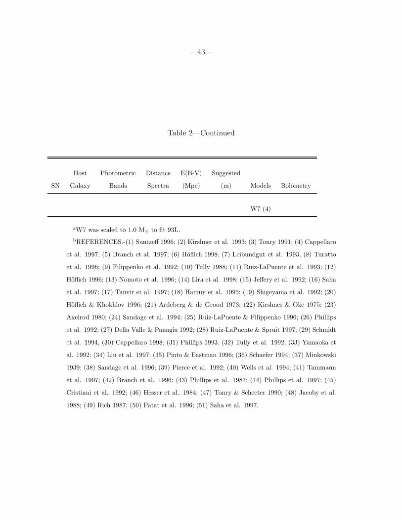
– 43 –

Table 2—Continued

Host Photometric Distance E(B-V) Suggested

SN Galaxy Bands Spectra (Mpc) (m) Models Bolometry

W7 (4)

aW7 was scaled to 1.0 M⊙ to fit 93L.

bREFERENCES.-(1) Suntzeff 1996; (2) Kirshner et al. 1993; (3) Tonry 1991; (4) Cappellaro

et al. 1997; (5) Branch et al. 1997; (6) Hoflich 1998; (7) Leibundgut et al. 1993; (8) Turatto

et al. 1996; (9) Filippenko et al. 1992; (10) Tully 1988; (11) Ruiz-LaPuente et al. 1993; (12)

Hoflich 1996; (13) Nomoto et al. 1996; (14) Lira et al. 1998; (15) Jeffery et al. 1992; (16) Saha

et al. 1997; (17) Tanvir et al. 1997; (18) Hamuy et al. 1995; (19) Shigeyama et al. 1992; (20)

Hoflich & Khokhlov 1996; (21) Ardeberg & de Grood 1973; (22) Kirshner & Oke 1975; (23)

Axelrod 1980; (24) Sandage et al. 1994; (25) Ruiz-LaPuente & Filippenko 1996; (26) Phillips

et al. 1992; (27) Della Valle & Panagia 1992; (28) Ruiz-LaPuente & Spruit 1997; (29) Schmidt

et al. 1994; (30) Cappellaro 1998; (31) Phillips 1993; (32) Tully et al. 1992; (33) Yamaoka et

al. 1992; (34) Liu et al. 1997; (35) Pinto & Eastman 1996; (36) Schaefer 1994; (37) Minkowski

1939; (38) Sandage et al. 1996; (39) Pierce et al. 1992; (40) Wells et al. 1994; (41) Tammann

et al. 1997; (42) Branch et al. 1996; (43) Phillips et al. 1987; (44) Phillips et al. 1997; (45)

Cristiani et al. 1992; (46) Hesser et al. 1984; (47) Tonry & Schecter 1990; (48) Jacoby et al.

1988; (49) Rich 1987; (50) Patat et al. 1996; (51) Saha et al. 1997.

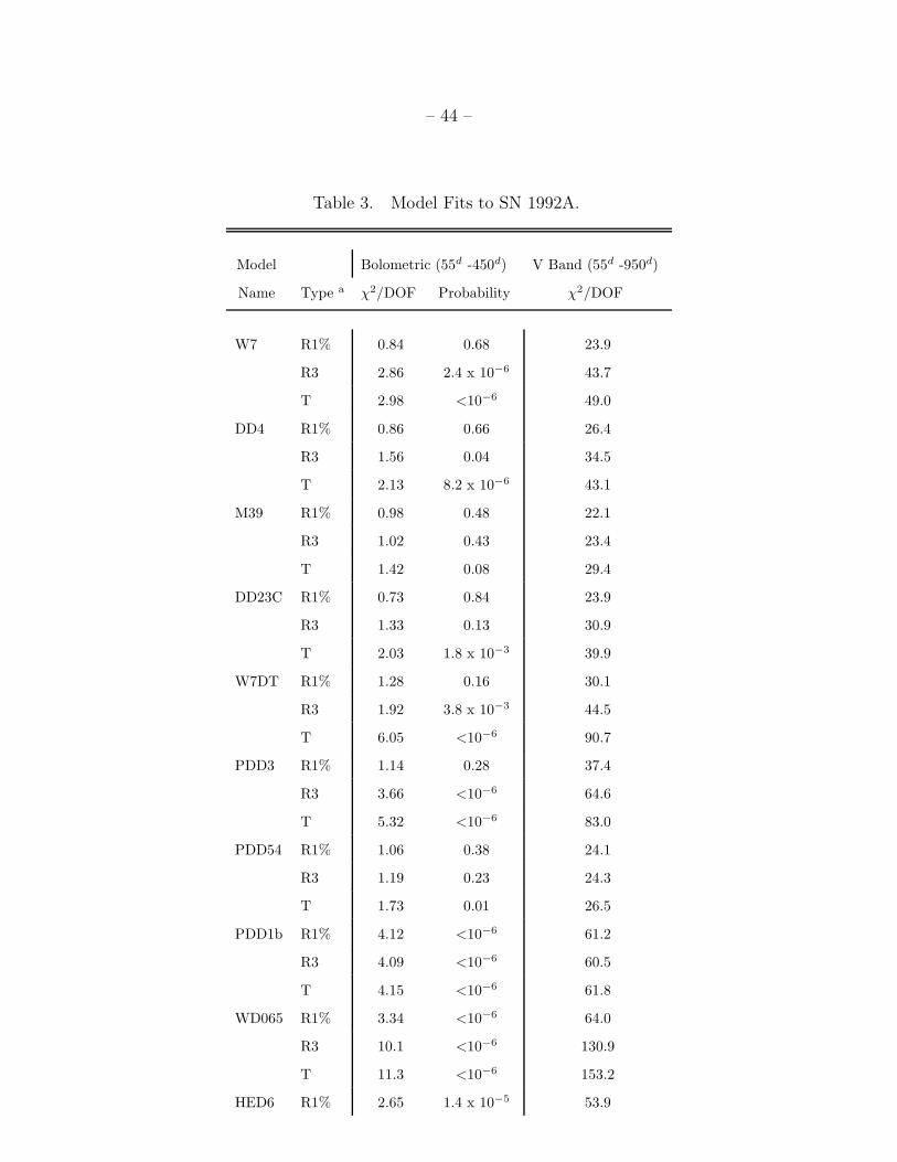
– 44 –

Table 3. Model Fits to SN 1992A.

Model Bolometric (55d -450d) V Band (55d -950d)

Name Type a χ2/DOF Probability χ2/DOF

W7 R1% 0.84 0.68 23.9

R3 2.86 2.4 x 10−6 43.7

T 2.98 <10−6 49.0

DD4 R1% 0.86 0.66 26.4

R3 1.56 0.04 34.5

T 2.13 8.2 x 10−6 43.1

M39 R1% 0.98 0.48 22.1

R3 1.02 0.43 23.4

T 1.42 0.08 29.4

DD23C R1% 0.73 0.84 23.9

R3 1.33 0.13 30.9

T 2.03 1.8 x 10−3 39.9

W7DT R1% 1.28 0.16 30.1

R3 1.92 3.8 x 10−3 44.5

T 6.05 <10−6 90.7

PDD3 R1% 1.14 0.28 37.4

R3 3.66 <10−6 64.6

T 5.32 <10−6 83.0

PDD54 R1% 1.06 0.38 24.1

R3 1.19 0.23 24.3

T 1.73 0.01 26.5

PDD1b R1% 4.12 <10−6 61.2

R3 4.09 <10−6 60.5

T 4.15 <10−6 61.8

WD065 R1% 3.34 <10−6 64.0

R3 10.1 <10−6 130.9

T 11.3 <10−6 153.2

HED6 R1% 2.65 1.4 x 10−5 53.9

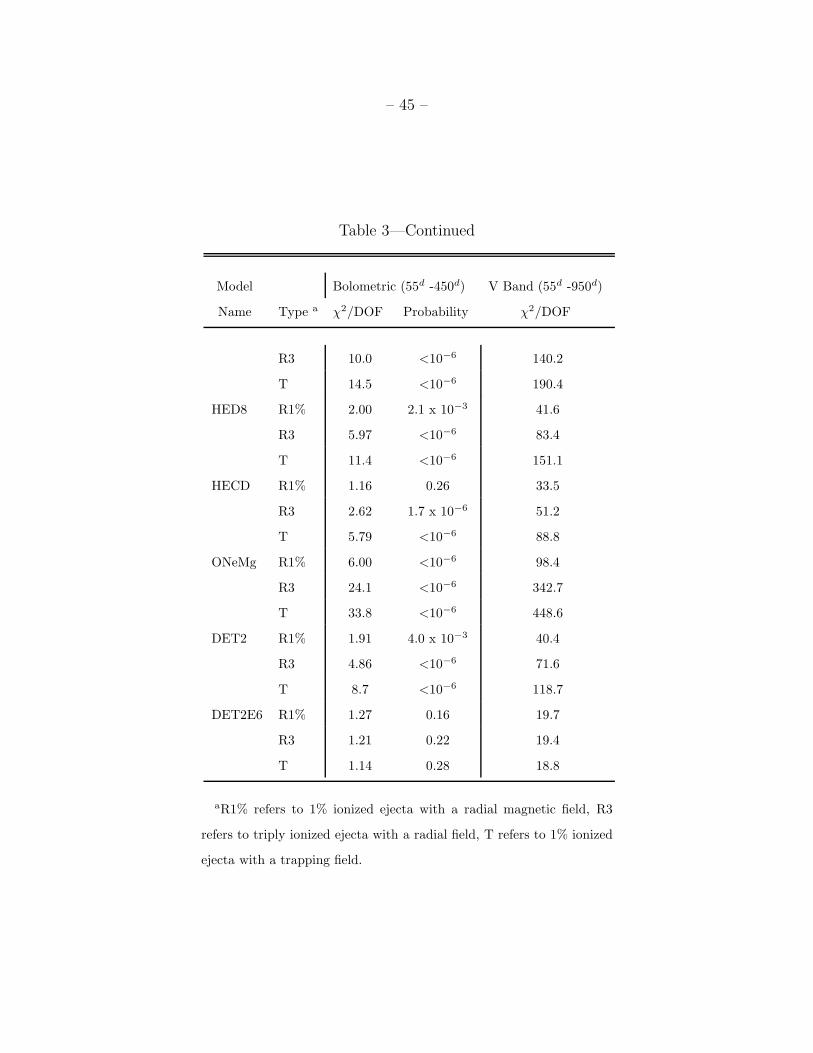
– 45 –

Table 3—Continued

Model Bolometric (55d -450d) V Band (55d -950d)

Name Type a χ2/DOF Probability χ2/DOF

R3 10.0 <10−6 140.2

T 14.5 <10−6 190.4

HED8 R1% 2.00 2.1 x 10−3 41.6

R3 5.97 <10−6 83.4

T 11.4 <10−6 151.1

HECD R1% 1.16 0.26 33.5

R3 2.62 1.7 x 10−6 51.2

T 5.79 <10−6 88.8

ONeMg R1% 6.00 <10−6 98.4

R3 24.1 <10−6 342.7

T 33.8 <10−6 448.6

DET2 R1% 1.91 4.0 x 10−3 40.4

R3 4.86 <10−6 71.6

T 8.7 <10−6 118.7

DET2E6 R1% 1.27 0.16 19.7

R3 1.21 0.22 19.4

T 1.14 0.28 18.8

aR1% refers to 1% ionized ejecta with a radial magnetic field, R3

refers to triply ionized ejecta with a radial field, T refers to 1% ionized

ejecta with a trapping field.

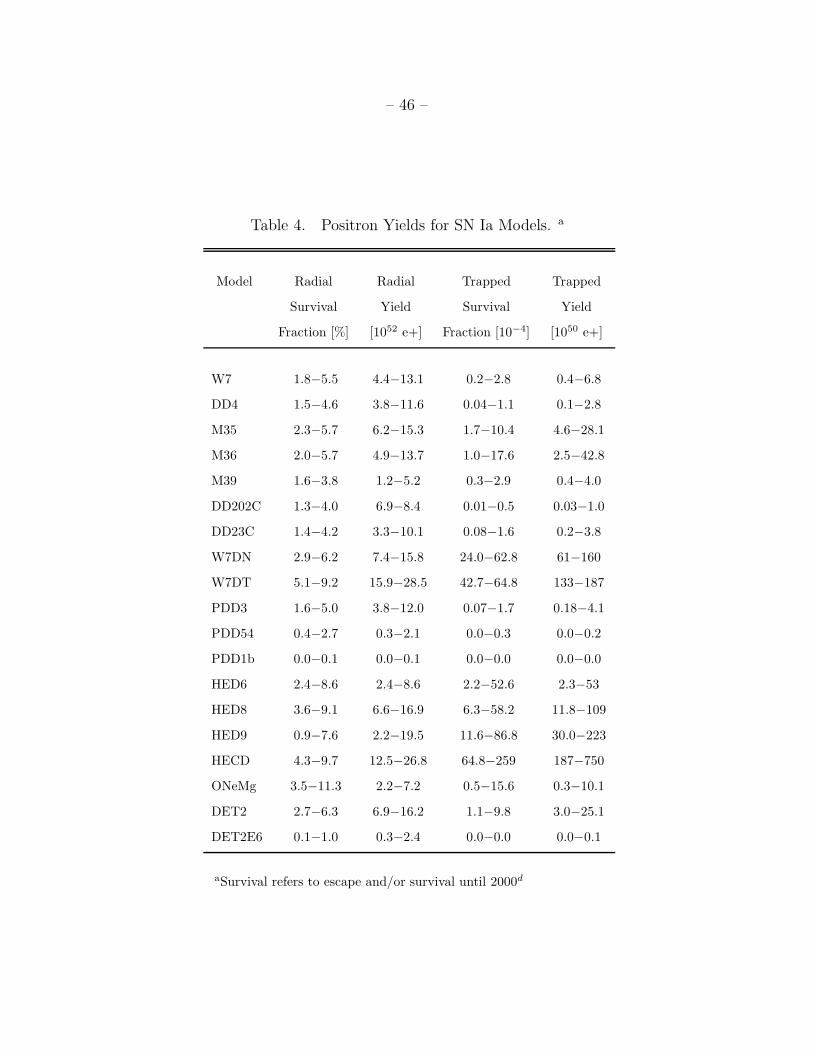
– 46 –

Table 4. Positron Yields for SN Ia Models. a

Model Radial Radial Trapped Trapped

Survival Yield Survival Yield

Fraction [%] [1052 e+] Fraction [10−4] [1050 e+]

W7 1.8−5.5 4.4−13.1 0.2−2.8 0.4−6.8

DD4 1.5−4.6 3.8−11.6 0.04−1.1 0.1−2.8

M35 2.3−5.7 6.2−15.3 1.7−10.4 4.6−28.1

M36 2.0−5.7 4.9−13.7 1.0−17.6 2.5−42.8

M39 1.6−3.8 1.2−5.2 0.3−2.9 0.4−4.0

DD202C 1.3−4.0 6.9−8.4 0.01−0.5 0.03−1.0

DD23C 1.4−4.2 3.3−10.1 0.08−1.6 0.2−3.8

W7DN 2.9−6.2 7.4−15.8 24.0−62.8 61−160

W7DT 5.1−9.2 15.9−28.5 42.7−64.8 133−187

PDD3 1.6−5.0 3.8−12.0 0.07−1.7 0.18−4.1

PDD54 0.4−2.7 0.3−2.1 0.0−0.3 0.0−0.2

PDD1b 0.0−0.1 0.0−0.1 0.0−0.0 0.0−0.0

HED6 2.4−8.6 2.4−8.6 2.2−52.6 2.3−53

HED8 3.6−9.1 6.6−16.9 6.3−58.2 11.8−109

HED9 0.9−7.6 2.2−19.5 11.6−86.8 30.0−223

HECD 4.3−9.7 12.5−26.8 64.8−259 187−750

ONeMg 3.5−11.3 2.2−7.2 0.5−15.6 0.3−10.1

DET2 2.7−6.3 6.9−16.2 1.1−9.8 3.0−25.1

DET2E6 0.1−1.0 0.3−2.4 0.0−0.0 0.0−0.1

aSurvival refers to escape and/or survival until 2000d

– 47 –

REFERENCES

Ahmad, I., Fischer, S.M., Bonino, G., Castagnoli, G.C., Kutschera, W., & Paul, M. 1997,

Phys. Rev. Lett., 80, 2550

Ardeberg A.L., & de Grood, M.J. 1973, A & A,28,295

Arnett, W.D. 1969, ApJ, 157, 1369

Arnett, W.D. 1980, ApJ, 237, 541

Arnett, W.D. 1982, ApJ, 253, 785

Axelrod, T.S. 1980, Ph.D. thesis, University of California at Santa Cruz

Baade, W. 1938, ApJ, 88, 285

Baade, W., & Zwicky, F. 1938, ApJ, 88, 411

Boffi, F.R. et al. 1998, BAAS, 192, 6.07

Bowers, E.J.C., Meikle, W.P.S., Geballe, T.R., Walton, N.A., Pinto, P.A., Dhillon, V.S.,

Howell, S.B., & Harrop-Allin, M.K. 1997, LANL, 9707119

Branch, D., Romanishin, W., & Baron, E. 1996,ApJ,465,73

Branch, D., Nugent, P., & Fisher, A. 1997 in Thermonuclear Supernovae, ed. P. Ruiz

Lapuente, R. Canal, & J. Isern (Dordrecht: Academic Publishers), 715

Burrows, A., & The, L.-S. 1990, ApJ, 360, 626

Capellaro, E., Mazzali, P., Benetti, S., Danziger I.J., Turatto, M., Della Valle, M., & Patat,

F. 1997, A&A,328, 203

– 48 –

Capellaro, E., Turatto, M., Tsvetkov, D.Yu., Bartunov, O.S., Pollas, C., Evans, R., &

Hamuy, M. 1997, A&A, 322, 431

Cappellaro, E., et al. 1998, unpublished

Chan, K.-W., & Lingenfelter, R.E. 1993, ApJ, 405, 614

Colgate, S. 1970, Ap&SS, 8, 457

Colgate, S., Petschek, A.G., & Kreise, J.T. 1980, ApJ, 237, L81

Colgate, S., Fryer, C.L., & Hand, K.P. 1996, in Thermonuclear Supernovae, ed. P. Ruiz

Lapuente, R. Canal, & J. Isern (Dordrecht: Academic Publishers), 273

Cristiani, S. et al. 1992, A&A, 259, 63

Della Valle, M. & Panagia, N. 1992,AJ,104,696

Filippenko, A.V., et al. 1992, AJ, 104, 1543

Filippenko, A.V., et al. 1992, ApJ, 384,L15

Fransson, C., Houck, J., & Kozma, C. 1996, in Supernovae and Supernova Remnants, IAU

Colloquium 145, eds. R. McCray & Z. Wang, p. 211

Hamuy, M., Phillips, M.M., Maza., J., Suntzeff, N.B., Schommer, R.A., & Aviles, R. 1995,

AJ, 109,1

Hamuy, M., Pinto, P.A. 1998, LANL, 9812084

Hesser, J.E., Harris, H.C., van den Bergh, S., & Harris, G.L.H. 1984, ApJ, 276, 491

Hoflich, P., Muller, E., & Khokhlov, A. 1993, A & A, 268, 570

Hoflich et al. 1996, ApJ,472, L81

– 49 –

Hoflich, P., & Khokhlov, A. 1996, ApJ, 457, 500

Hoflich, P. 1996, in Supernovae and Supernova Remnants, IAU Colloquium 145, eds. R.

McCray & Z. Wang, p. 29

Hoflich, P. 1995, ApJ, 443, 89

Hoflich, P., Wheeler, J. C., & Thielemann, F.-K. 1998, ApJ, 495, 617

Hoflich, P., Private Communication

Hoyle, F. & Fowler, W. A. 1960, ApJ, 132, 565

Stopping Powers for Electrons and Positrons, International Commission on Radiation Units

and Measurements Report; 37 1984

Jacoby, G.H., Ciardullo, R., & Ford, H.C. 1988, in The Extragalactic Distance Scale, BYU

Press

Jeffery, D.J., Leibundgut, B., Kirshner, R.P., Benetti, S., Branch, D., & Sonneborn, G.

1992, ApJ, 397, 304

Jeffery, D.J. 1998, private communication

Kirshner, R.P., & Oke, J.B. 1975, ApJ, 200, 574

Kirshner, R.P., et al. 1993, ApJ, 415, 589

Kumagai, S. 1997, private communication

Leibundgut, B., Kirshner, R.P., Filippenko, A.V., Shields, J.C., Foltz, C.B., Phillips, M.M.,

& Sonneborn, G. 1991, ApJ, 371, L23

Leibundgut, B. & Pinto, P.A. 1992, ApJ, 401, 49

– 50 –

Leibundgut, B., et al. 1993, AJ, 105,301

Leising, M.D., Johnson, W.N., Kurfess, J.D., Clayton, D.D., Grabelsky, D.A., Jung, G.V.,

Kinzer, R.L., Purcell, W.R., Strickman, M.S., The L.-S., & Ulmer, M.P. 1995, ApJ,

450, 805

Lira, P. Master’s Thesis, University of Chile

Lira, P., et al. 1998,AJ,115,234

Liu, W., Jeffery, D.J., & Schultz, D.R. 1997, ApJ,483,L107

Liu, W., Jeffery, D.J., & Schultz, D.R. 1997, ApJ,486,L35

Liu, W., Jeffery, D.J., & Schultz, D.R. 1998, ApJ,494,812

Mazzali, P.A., et al. 1996, MNRAS, 284, 151

Milne, P.A. 1998, PhD thesis, Clemson University

Milne, P.A., Kurfess, J.D., & Leising, M.D. 1999, in preparation

Minkowski, R. 1939, ApJ, 89, 143

Nomoto, K., Thielemann, F.-K., & Yokoi, K. 1984, ApJ, 286, 644

Nomoto K. et al. 1996, in Supernovae and Supernova Remnants, IAU Colloquium 145, eds.

R. McCray & Z. Wang, p. 49

Patat, F., Benetti, S., Cappellaro, E., Danziger, I.J., Della Valle, M., Mazzali, P.A., &

Turatto, M. 1996, MNRAS,278,111

Phillips, M.M., et al. 1987,PASP, 99, 592

Phillips, M.M., Jacoby, G.H., Walker, A.R., Tonry, J.L. & Ciardullo, R. 1992, BAAS, 24,749

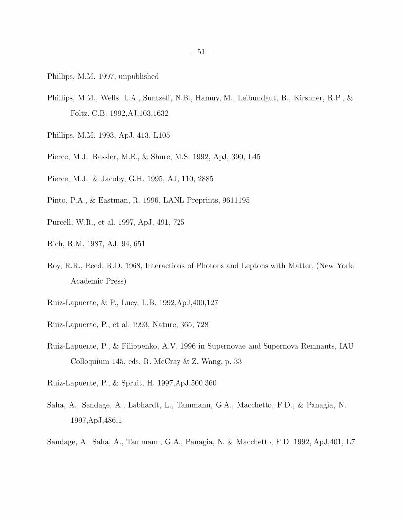
– 51 –

Phillips, M.M. 1997, unpublished

Phillips, M.M., Wells, L.A., Suntzeff, N.B., Hamuy, M., Leibundgut, B., Kirshner, R.P., &

Foltz, C.B. 1992,AJ,103,1632

Phillips, M.M. 1993, ApJ, 413, L105

Pierce, M.J., Ressler, M.E., & Shure, M.S. 1992, ApJ, 390, L45

Pierce, M.J., & Jacoby, G.H. 1995, AJ, 110, 2885

Pinto, P.A., & Eastman, R. 1996, LANL Preprints, 9611195

Purcell, W.R., et al. 1997, ApJ, 491, 725

Rich, R.M. 1987, AJ, 94, 651

Roy, R.R., Reed, R.D. 1968, Interactions of Photons and Leptons with Matter, (New York:

Academic Press)

Ruiz-Lapuente, & P., Lucy, L.B. 1992,ApJ,400,127

Ruiz-Lapuente, P., et al. 1993, Nature, 365, 728

Ruiz-Lapuente, P., & Filippenko, A.V. 1996 in Supernovae and Supernova Remnants, IAU

Colloquium 145, eds. R. McCray & Z. Wang, p. 33

Ruiz-Lapuente, P., & Spruit, H. 1997,ApJ,500,360

Saha, A., Sandage, A., Labhardt, L., Tammann, G.A., Macchetto, F.D., & Panagia, N.

1997,ApJ,486,1

Sandage, A., Saha, A., Tammann, G.A., Panagia, N. & Macchetto, F.D. 1992, ApJ,401, L7

– 52 –

Sandage, A., Saha, A., Tammann, G.A., Labhardt, L., Schwengeler, H., Panagia, N. &

Macchetto, F.D. 1994, ApJ, 423,L13

Sandage, A., Carlson, G., Kristian, J., Saha, A., & Labhardt, L. 1996, AJ, 111, 1872

Schaefer, B.E. 1994, ApJ,426,493

Schmidt,B.P., Kirshner,R.P., Leibundgut, B., Wells, L.A., Porter, A.C., Ruiz-Lapuente, P.,

Challis, & P., Filippenko, A.V. 1994, ApJ, 434, L19

Segre, E. 1977, Nuclei and Particles, (New York: Benjamin/Cummings)

Shigeyama, T., Nomoto, K., Yamaoka, H., & Thielemann, F.-K. 1992, ApJ,386,L13

Suntzeff, N.B., 1996, in Supernovae and Supernova Remnants, ed. R. McCray, Z. Wang

(Cambridge:Cambridge Press), p. 41

Suntzeff, N.B., Phillips, M.M., et al. 1998, LANL, 9811205

Tammann, G.A., Sandage, A., Saha, A., Labhardt, L, Macchetto, F.D., & Panagia, N. 1997,

in Thermonuclear Supernovae, ed. P. Ruiz Lapuente, R. Canal, J. Isern (Dordrecht:

Academic Publishers), 735

Tanvir, N., Shanks, T., Dhillon, V., Lucy, J., Morris, P., Knapen, J., Balcells, M., Irwin,

M., Casteneda, H., & Walton, N. 1997, unpublished

The, L.-S., Bridgeman, W. & Clayton, D.D. 1994, ApJS, 93, 531

The, L.-S., Burrows, A., & Bussard, R. 1990, ApJ, 352, 731

Tonry, J.L. 1991, ApJ, 373, L1

Tonry, J.L., & Schechter, P.L. 1990, AJ, 100, 1794

Tully, R.B. 1988, Nearby Galaxy Catalog, Cambridge Univ. Press, Cambridge

– 53 –

Tully, R.B., Shaya, E.J., & Pierce, M.J. 1992, ApJS, 80, 479

Turatto, M.,Benetti, I.J., Capellaro, E., Danziger, I.J., Della Valle, M., Gouiffes, C.,

Mazzali, P., & Patat, F. 1996, MNRAS, 283, 1

Wells, L.A., et al. 1994,AJ,106,2233

Woosley, S. E. & Weaver, T. A., 1986, ARA&A, 24, 205

Yamaoka, H., Nomoto, K., Shigeyama, T., & Thielemann, F.-K. 1992, ApJ, 393, L55

This manuscript was prepared with the AAS LATEX macros v4.0.

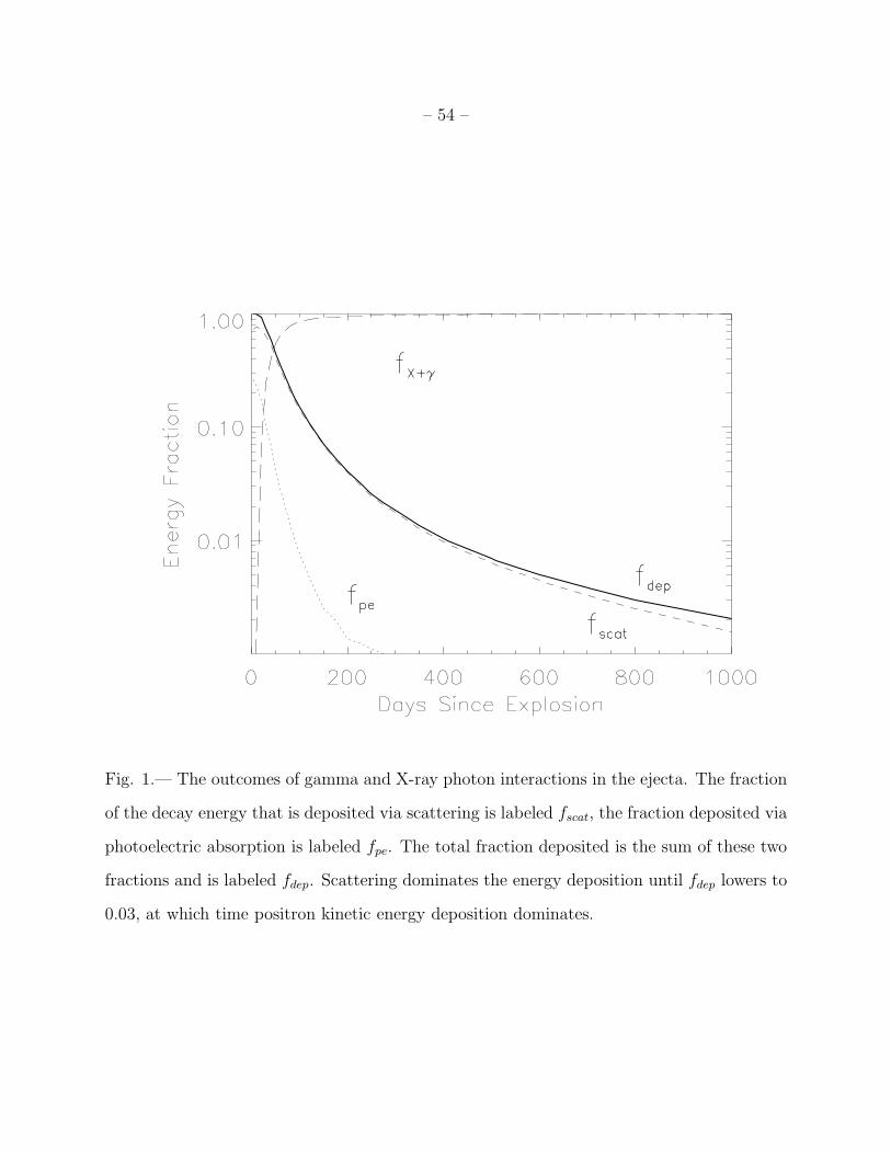
– 54 –

Fig. 1.— The outcomes of gamma and X-ray photon interactions in the ejecta. The fraction

of the decay energy that is deposited via scattering is labeled fscat, the fraction deposited via

photoelectric absorption is labeled fpe. The total fraction deposited is the sum of these two

fractions and is labeled fdep. Scattering dominates the energy deposition until fdep lowers to

0.03, at which time positron kinetic energy deposition dominates.

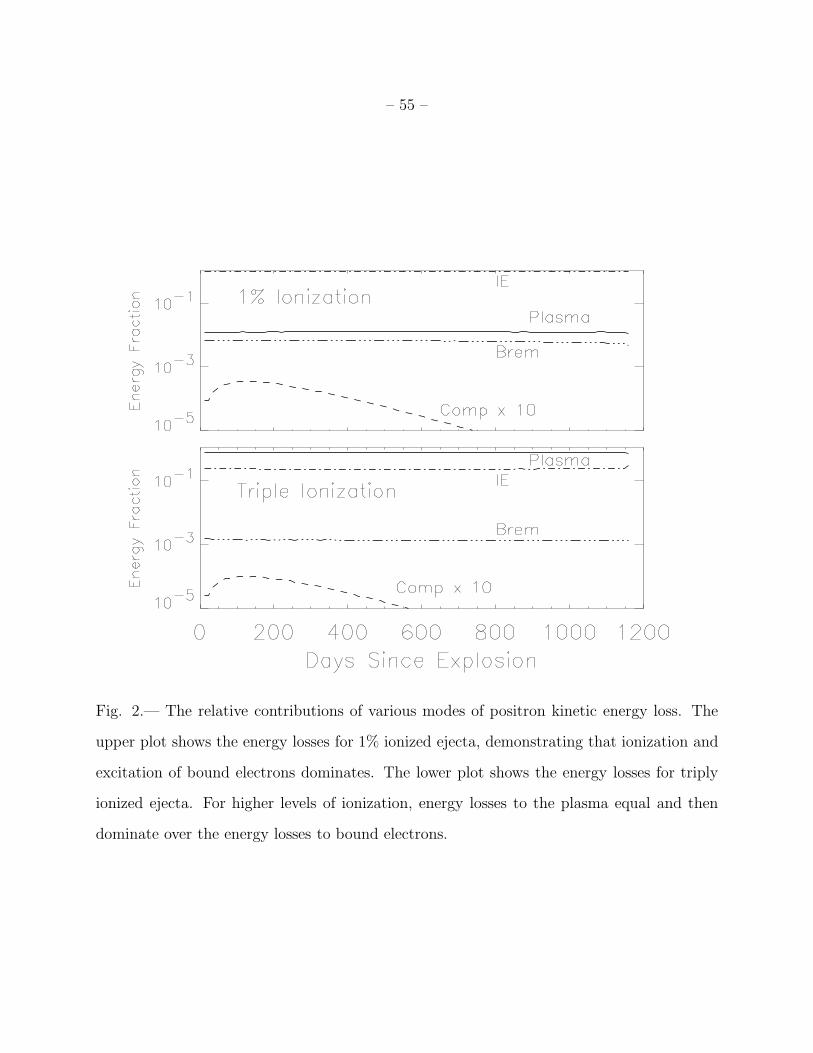
– 55 –

Fig. 2.— The relative contributions of various modes of positron kinetic energy loss. The

upper plot shows the energy losses for 1% ionized ejecta, demonstrating that ionization and

excitation of bound electrons dominates. The lower plot shows the energy losses for triply

ionized ejecta. For higher levels of ionization, energy losses to the plasma equal and then

dominate over the energy losses to bound electrons.

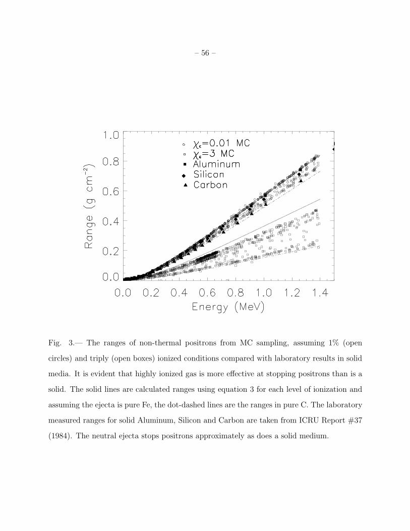
– 56 –

Fig. 3.— The ranges of non-thermal positrons from MC sampling, assuming 1% (open

circles) and triply (open boxes) ionized conditions compared with laboratory results in solid

media. It is evident that highly ionized gas is more effective at stopping positrons than is a

solid. The solid lines are calculated ranges using equation 3 for each level of ionization and

assuming the ejecta is pure Fe, the dot-dashed lines are the ranges in pure C. The laboratory

measured ranges for solid Aluminum, Silicon and Carbon are taken from ICRU Report #37

(1984). The neutral ejecta stops positrons approximately as does a solid medium.

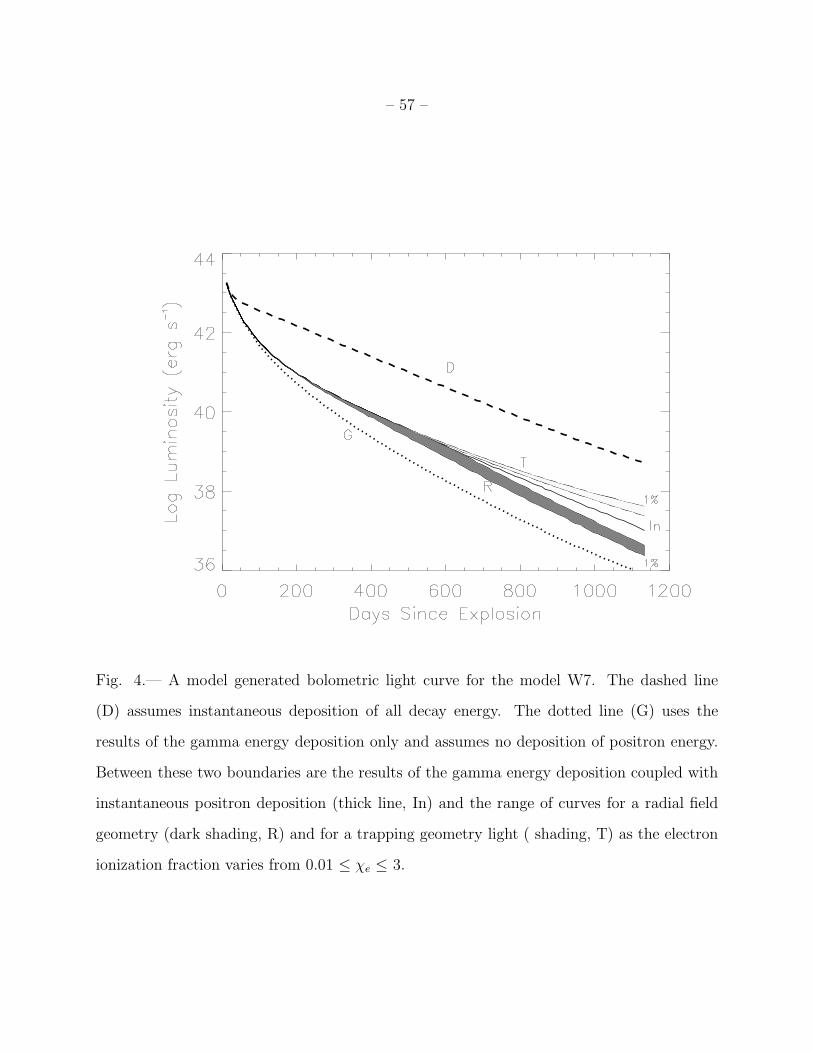
– 57 –

Fig. 4.— A model generated bolometric light curve for the model W7. The dashed line

(D) assumes instantaneous deposition of all decay energy. The dotted line (G) uses the

results of the gamma energy deposition only and assumes no deposition of positron energy.

Between these two boundaries are the results of the gamma energy deposition coupled with

instantaneous positron deposition (thick line, In) and the range of curves for a radial field

geometry (dark shading, R) and for a trapping geometry light ( shading, T) as the electron

ionization fraction varies from 0.01 ≤ χe ≤ 3.

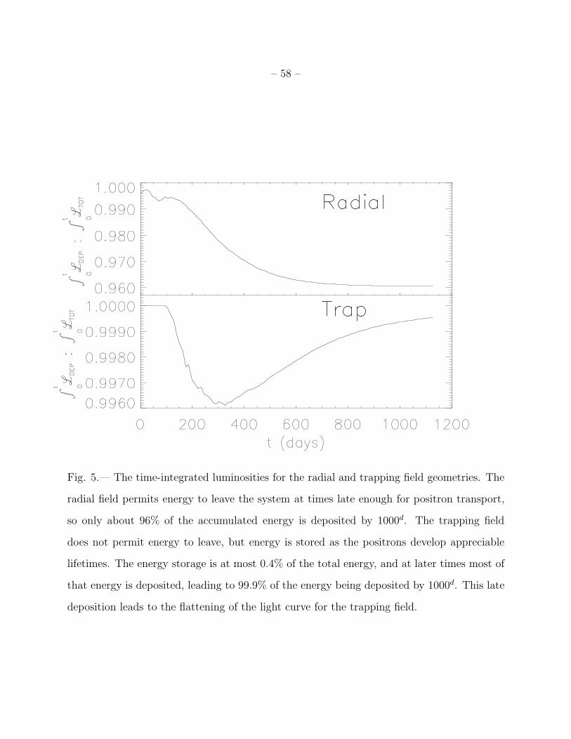
– 58 –

Fig. 5.— The time-integrated luminosities for the radial and trapping field geometries. The

radial field permits energy to leave the system at times late enough for positron transport,

so only about 96% of the accumulated energy is deposited by 1000d. The trapping field

does not permit energy to leave, but energy is stored as the positrons develop appreciable

lifetimes. The energy storage is at most 0.4% of the total energy, and at later times most of

that energy is deposited, leading to 99.9% of the energy being deposited by 1000d. This late

deposition leads to the flattening of the light curve for the trapping field.

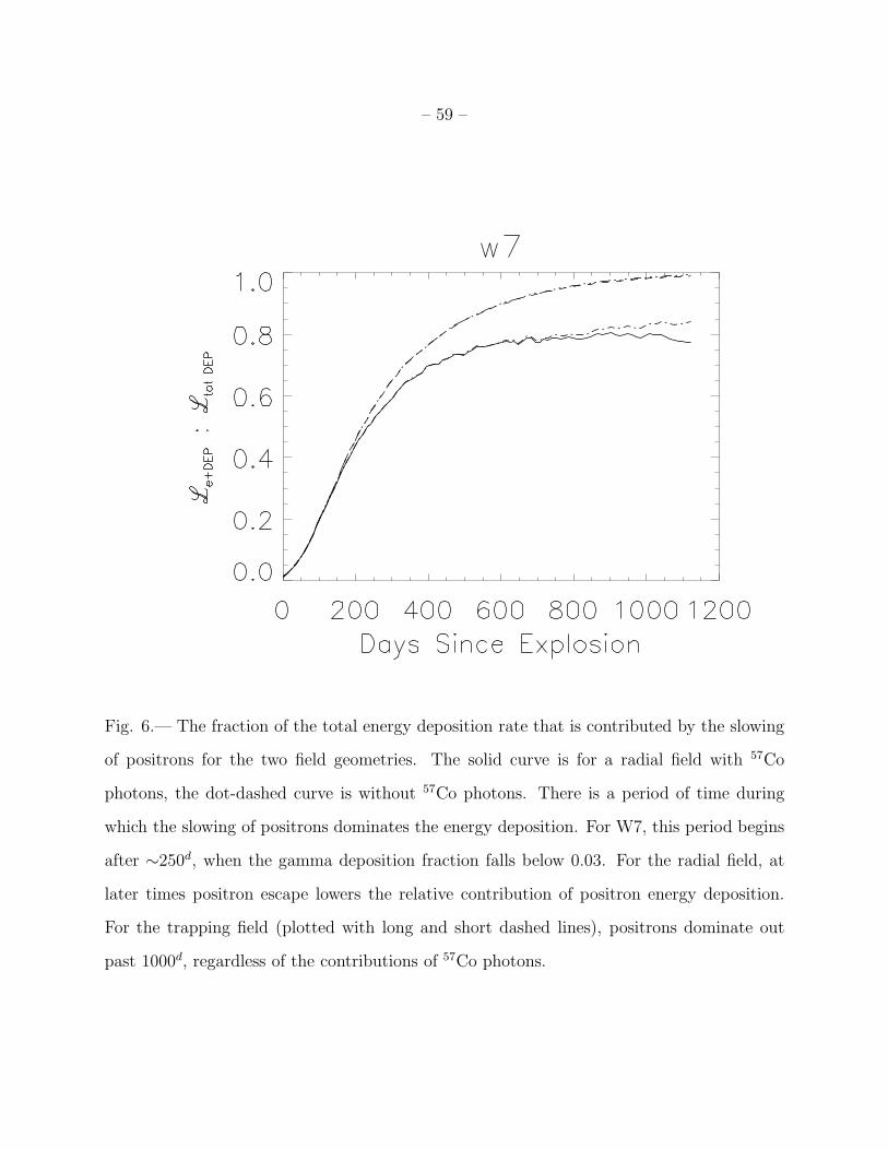
– 59 –

Fig. 6.— The fraction of the total energy deposition rate that is contributed by the slowing

of positrons for the two field geometries. The solid curve is for a radial field with 57Co

photons, the dot-dashed curve is without 57Co photons. There is a period of time during

which the slowing of positrons dominates the energy deposition. For W7, this period begins

after ∼250d, when the gamma deposition fraction falls below 0.03. For the radial field, at

later times positron escape lowers the relative contribution of positron energy deposition.

For the trapping field (plotted with long and short dashed lines), positrons dominate out

past 1000d, regardless of the contributions of 57Co photons.

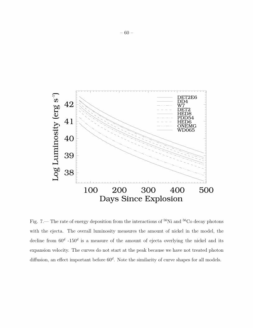
– 60 –

100 200 300 400 500Days Since Explosion

38

39

40

41

42

Log L

um

inosit

y (erg

s-1)

WD065ONEMGHED6PDD54HED8DET2W7DD4DET2E6

Fig. 7.— The rate of energy deposition from the interactions of 56Ni and 56Co decay photons

with the ejecta. The overall luminosity measures the amount of nickel in the model, the

decline from 60d -150d is a measure of the amount of ejecta overlying the nickel and its

expansion velocity. The curves do not start at the peak because we have not treated photon

diffusion, an effect important before 60d. Note the similarity of curve shapes for all models.

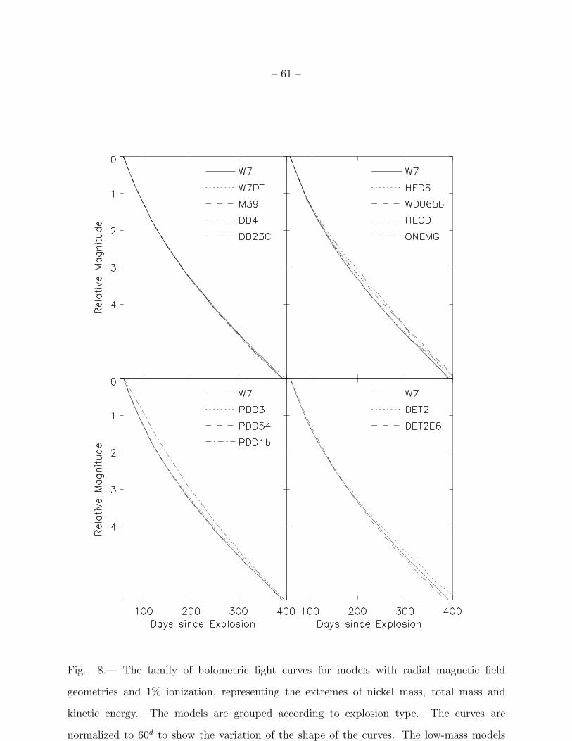
– 61 –

Fig. 8.— The family of bolometric light curves for models with radial magnetic field

geometries and 1% ionization, representing the extremes of nickel mass, total mass and

kinetic energy. The models are grouped according to explosion type. The curves are

normalized to 60d to show the variation of the shape of the curves. The low-mass models

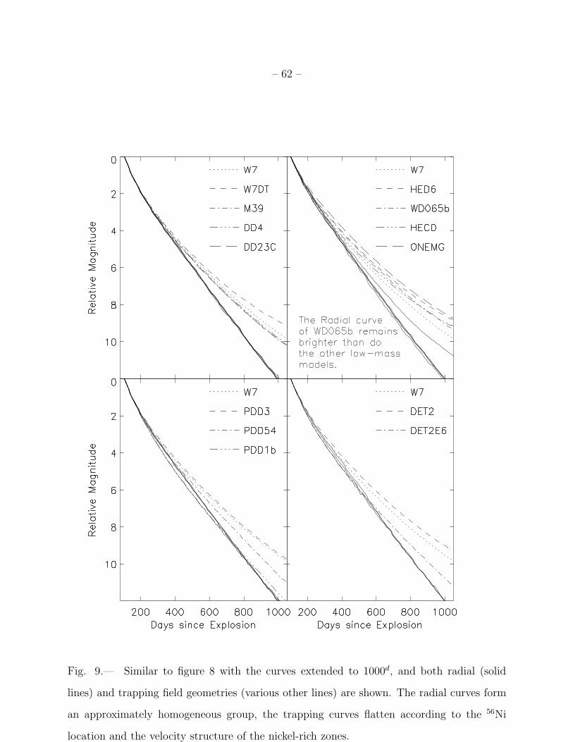
– 62 –

Fig. 9.— Similar to figure 8 with the curves extended to 1000d, and both radial (solid

lines) and trapping field geometries (various other lines) are shown. The radial curves form

an approximately homogeneous group, the trapping curves flatten according to the 56Ni

location and the velocity structure of the nickel-rich zones.

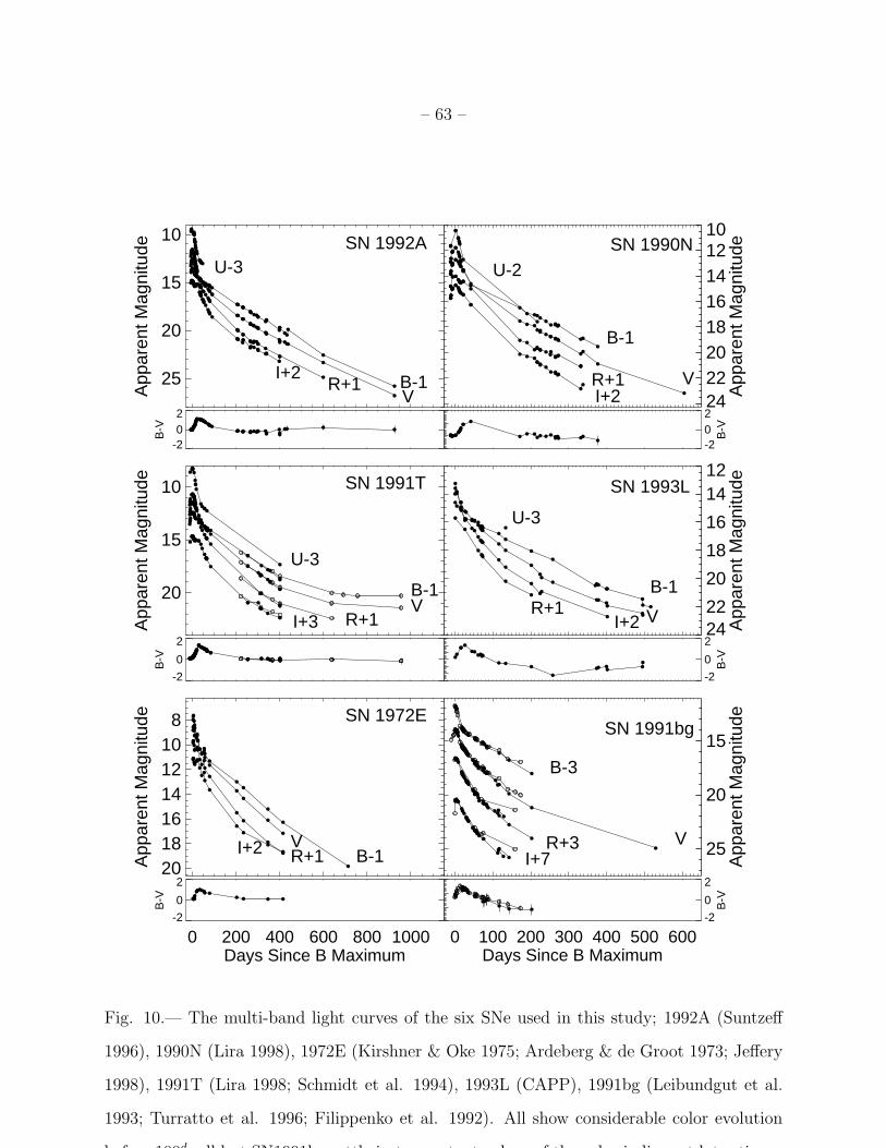
– 63 –

25

20

15

10

App

aren

t Mag

nitu

de

U-3

B-1V

R+1I+2

SN 1992A

-202

B-V

2422201816141210

App

aren

t Mag

nitu

de

U-2

B-1

VR+1I+2

SN 1990N

-202

B-V

20

15

10

App

aren

t Mag

nitu

de

U-3

B-1V

R+1I+3

SN 1991T

-2

0

2

B-V

2422

20

18

16

1412

App

aren

t Mag

nitu

de

U-3

B-1

VR+1I+2

SN 1993L

-2

0

2

B-V

2018161412108

App

aren

t Mag

nitu

de

B-1VR+1I+2

SN 1972E

0 200 400 600 800 1000Days Since B Maximum

-2

0

2

B-V

25

20

15A

ppar

ent M

agni

tude

B-3

VR+3I+7

SN 1991bg

0 100 200 300 400 500 600Days Since B Maximum

-2

0

2

B-V

Fig. 10.— The multi-band light curves of the six SNe used in this study; 1992A (Suntzeff

1996), 1990N (Lira 1998), 1972E (Kirshner & Oke 1975; Ardeberg & de Groot 1973; Jeffery

1998), 1991T (Lira 1998; Schmidt et al. 1994), 1993L (CAPP), 1991bg (Leibundgut et al.

1993; Turratto et al. 1996; Filippenko et al. 1992). All show considerable color evolution

before 100d, all but SN1991bg settle in to constant values of the color indices at later times.

– 64 –

Fig. 11.— The bolometric magnitudes (solid lines) of five SNe compared with the V (dashed

lines) and B (dot-dashed lines) band data.

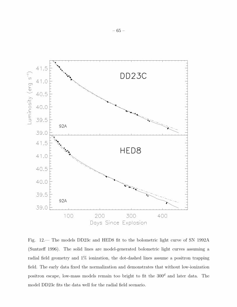
– 65 –

Fig. 12.— The models DD23c and HED8 fit to the bolometric light curve of SN 1992A

(Suntzeff 1996). The solid lines are model-generated bolometric light curves assuming a

radial field geometry and 1% ionization, the dot-dashed lines assume a positron trapping

field. The early data fixed the normalization and demonstrates that without low-ionization

positron escape, low-mass models remain too bright to fit the 300d and later data. The

model DD23c fits the data well for the radial field scenario.

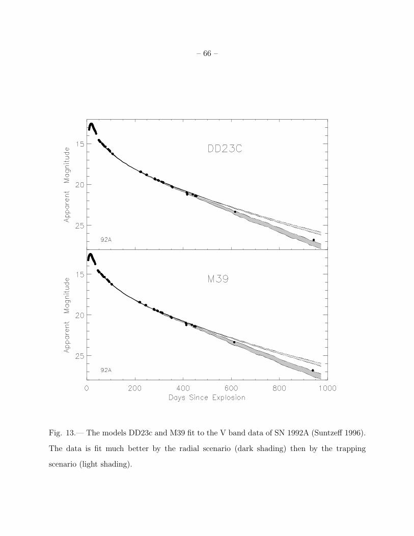
– 66 –

Fig. 13.— The models DD23c and M39 fit to the V band data of SN 1992A (Suntzeff 1996).

The data is fit much better by the radial scenario (dark shading) then by the trapping

scenario (light shading).

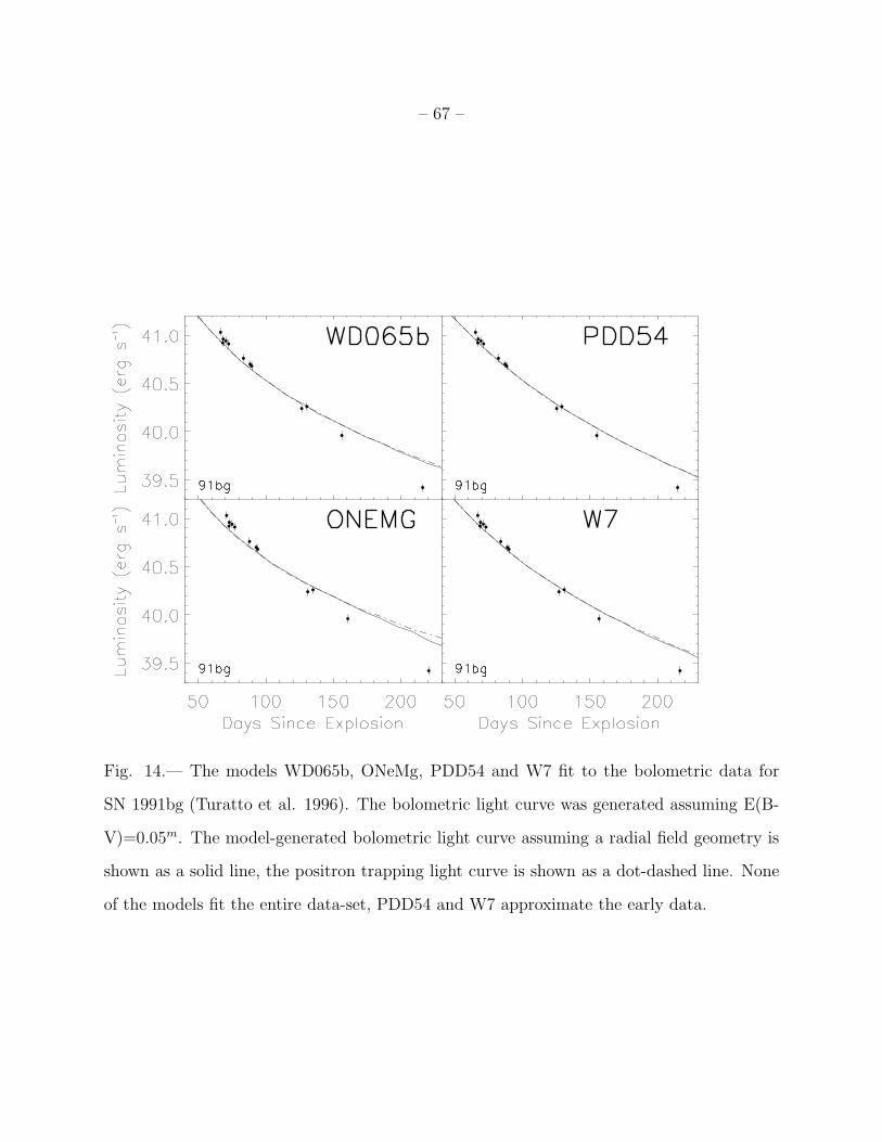
– 67 –

Fig. 14.— The models WD065b, ONeMg, PDD54 and W7 fit to the bolometric data for

SN 1991bg (Turatto et al. 1996). The bolometric light curve was generated assuming E(B-

V)=0.05m. The model-generated bolometric light curve assuming a radial field geometry is

shown as a solid line, the positron trapping light curve is shown as a dot-dashed line. None

of the models fit the entire data-set, PDD54 and W7 approximate the early data.

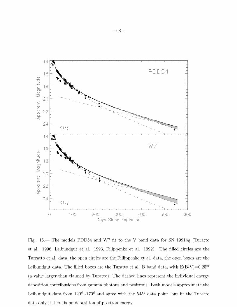
– 68 –

Fig. 15.— The models PDD54 and W7 fit to the V band data for SN 1991bg (Turatto

et al. 1996, Leibundgut et al. 1993, Filippenko et al. 1992). The filled circles are the

Turratto et al. data, the open circles are the Fillippenko et al. data, the open boxes are the

Leibundgut data. The filled boxes are the Turatto et al. B band data, with E(B-V)=0.25m

(a value larger than claimed by Turatto). The dashed lines represent the individual energy

deposition contributions from gamma photons and positrons. Both models approximate the

Leibundgut data from 120d -170d and agree with the 545d data point, but fit the Turatto

data only if there is no deposition of positron energy.

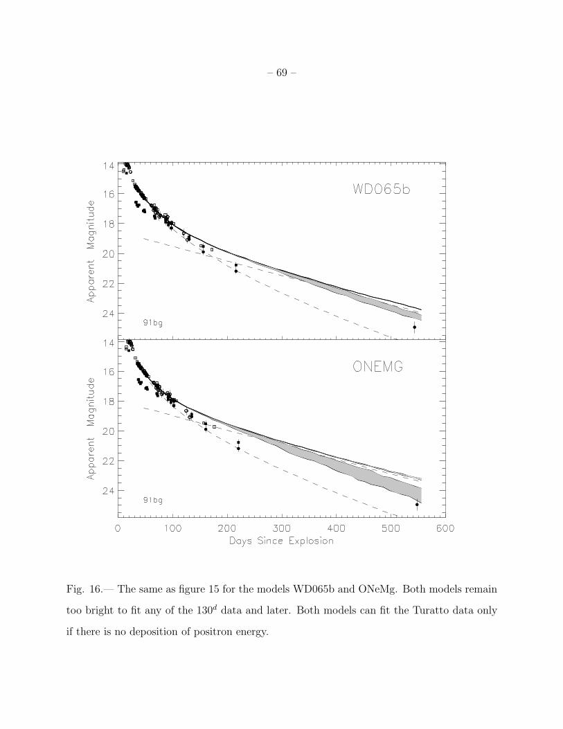
– 69 –

Fig. 16.— The same as figure 15 for the models WD065b and ONeMg. Both models remain

too bright to fit any of the 130d data and later. Both models can fit the Turatto data only

if there is no deposition of positron energy.

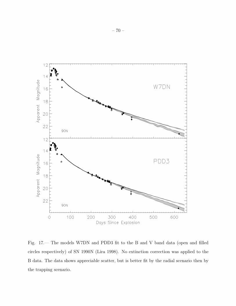
– 70 –

Fig. 17.— The models W7DN and PDD3 fit to the B and V band data (open and filled

circles respectively) of SN 1990N (Lira 1998). No extinction correction was applied to the

B data. The data shows appreciable scatter, but is better fit by the radial scenario then by

the trapping scenario.

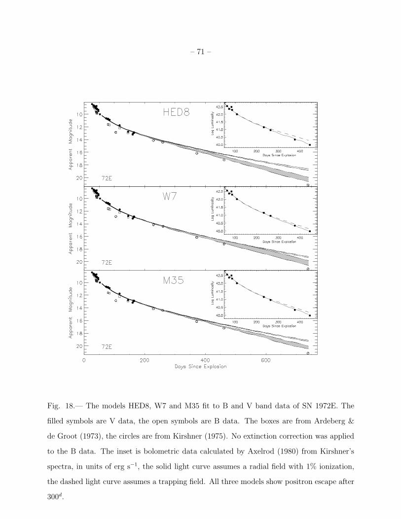
– 71 –

Fig. 18.— The models HED8, W7 and M35 fit to B and V band data of SN 1972E. The

filled symbols are V data, the open symbols are B data. The boxes are from Ardeberg &

de Groot (1973), the circles are from Kirshner (1975). No extinction correction was applied

to the B data. The inset is bolometric data calculated by Axelrod (1980) from Kirshner’s

spectra, in units of erg s−1, the solid light curve assumes a radial field with 1% ionization,

the dashed light curve assumes a trapping field. All three models show positron escape after

300d.

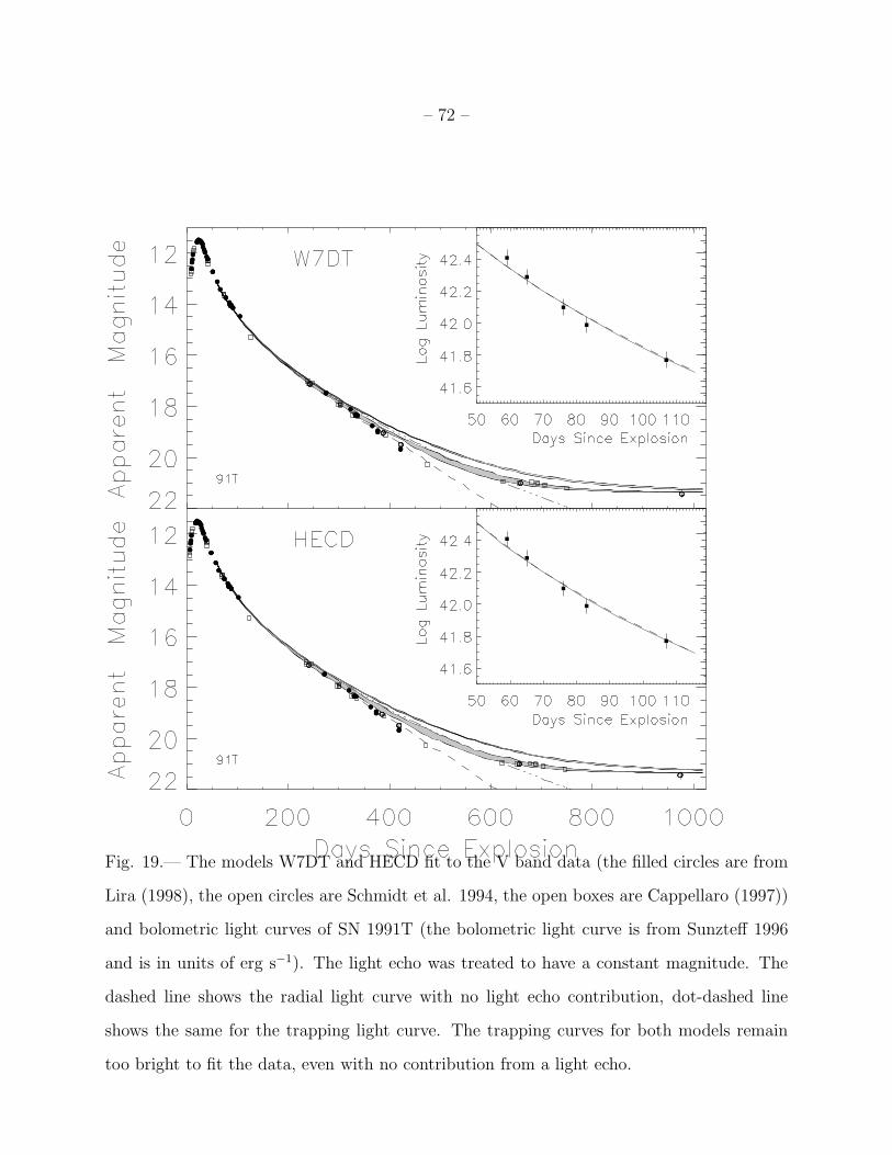
– 72 –

Fig. 19.— The models W7DT and HECD fit to the V band data (the filled circles are from

Lira (1998), the open circles are Schmidt et al. 1994, the open boxes are Cappellaro (1997))

and bolometric light curves of SN 1991T (the bolometric light curve is from Sunzteff 1996

and is in units of erg s−1). The light echo was treated to have a constant magnitude. The

dashed line shows the radial light curve with no light echo contribution, dot-dashed line

shows the same for the trapping light curve. The trapping curves for both models remain

too bright to fit the data, even with no contribution from a light echo.

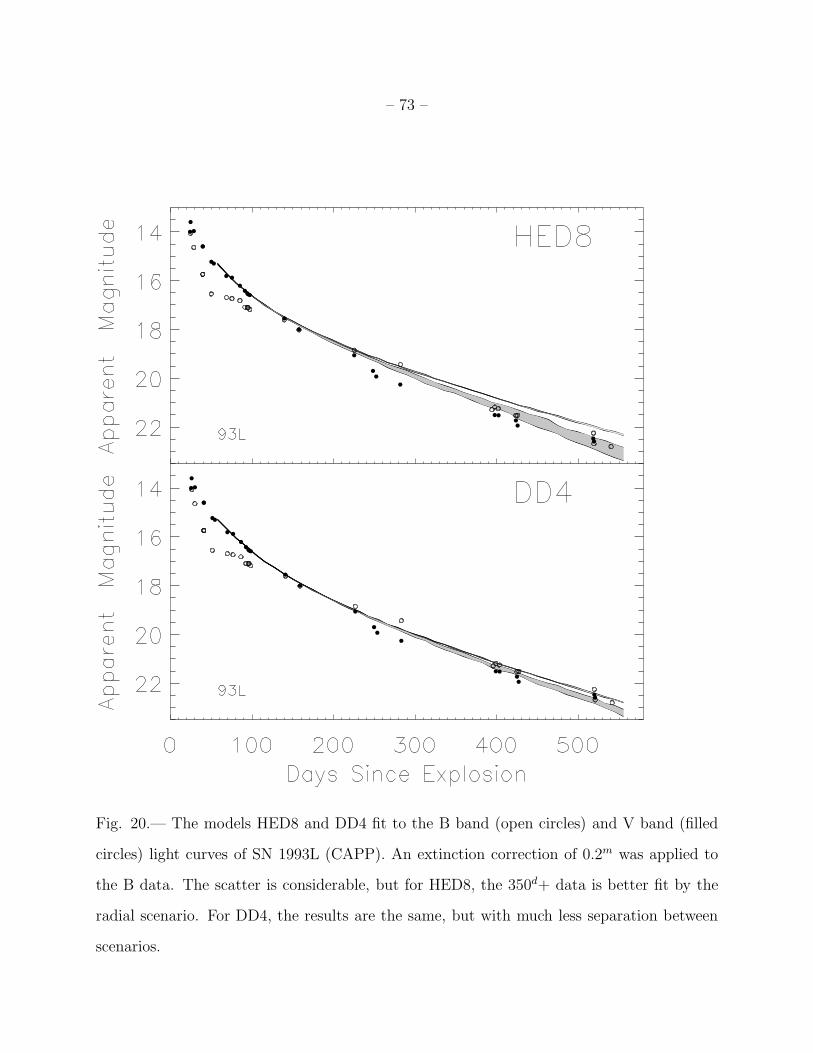
– 73 –

Fig. 20.— The models HED8 and DD4 fit to the B band (open circles) and V band (filled

circles) light curves of SN 1993L (CAPP). An extinction correction of 0.2m was applied to

the B data. The scatter is considerable, but for HED8, the 350d+ data is better fit by the

radial scenario. For DD4, the results are the same, but with much less separation between

scenarios.

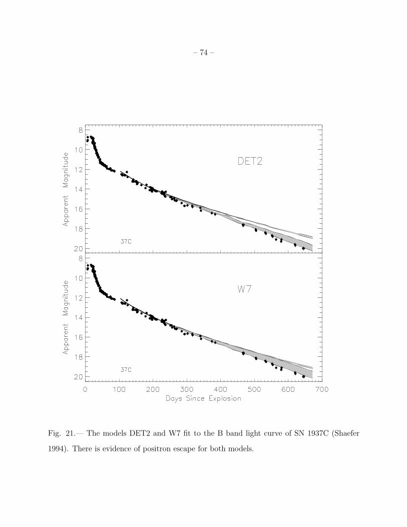
– 74 –

Fig. 21.— The models DET2 and W7 fit to the B band light curve of SN 1937C (Shaefer

1994). There is evidence of positron escape for both models.

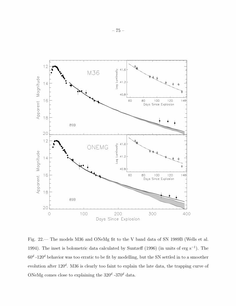
– 75 –

Fig. 22.— The models M36 and ONeMg fit to the V band data of SN 1989B (Wells et al.

1994). The inset is bolometric data calculated by Suntzeff (1996) (in units of erg s−1). The

60d -120d behavior was too erratic to be fit by modelling, but the SN settled in to a smoother

evolution after 120d. M36 is clearly too faint to explain the late data, the trapping curve of

ONeMg comes close to explaining the 320d -370d data.

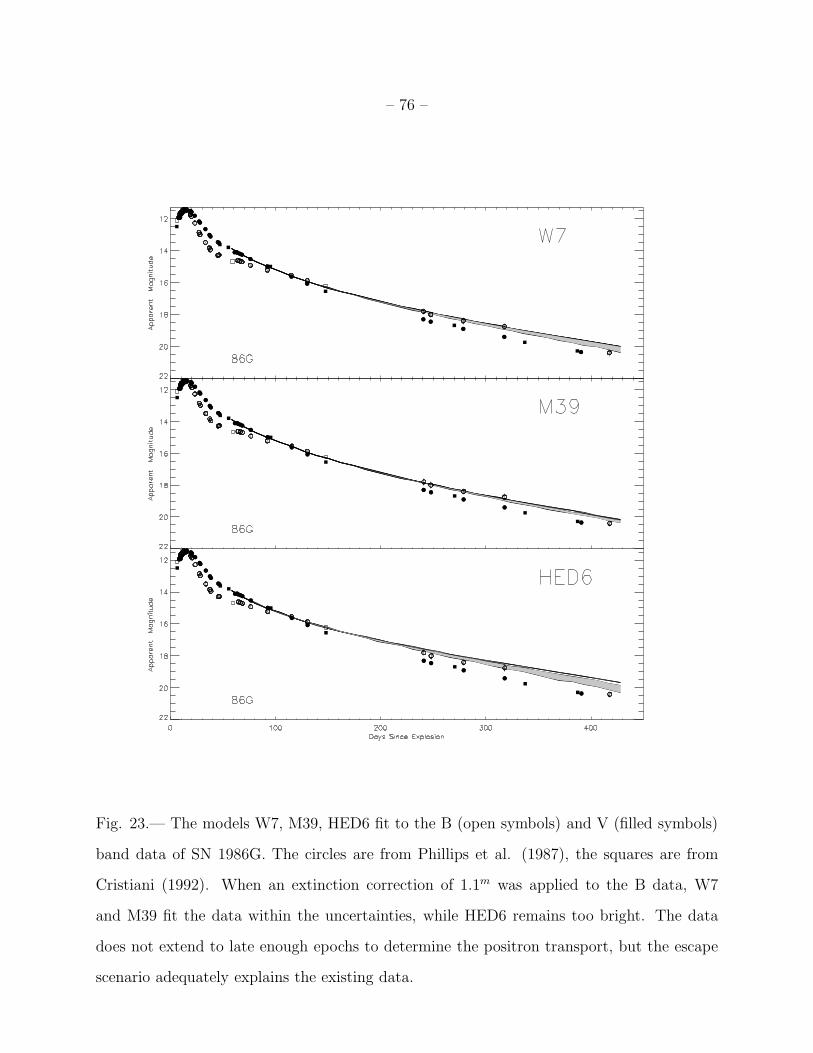
– 76 –

Fig. 23.— The models W7, M39, HED6 fit to the B (open symbols) and V (filled symbols)

band data of SN 1986G. The circles are from Phillips et al. (1987), the squares are from

Cristiani (1992). When an extinction correction of 1.1m was applied to the B data, W7

and M39 fit the data within the uncertainties, while HED6 remains too bright. The data

does not extend to late enough epochs to determine the positron transport, but the escape

scenario adequately explains the existing data.

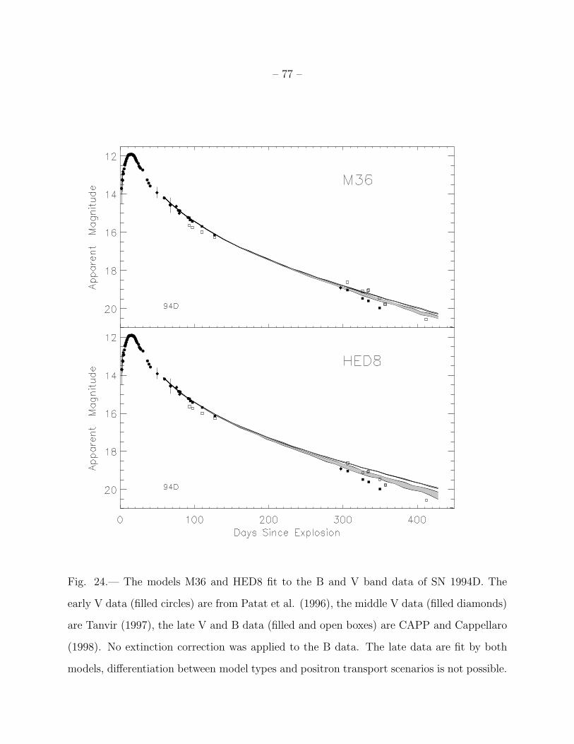
– 77 –

Fig. 24.— The models M36 and HED8 fit to the B and V band data of SN 1994D. The

early V data (filled circles) are from Patat et al. (1996), the middle V data (filled diamonds)

are Tanvir (1997), the late V and B data (filled and open boxes) are CAPP and Cappellaro

(1998). No extinction correction was applied to the B data. The late data are fit by both

models, differentiation between model types and positron transport scenarios is not possible.

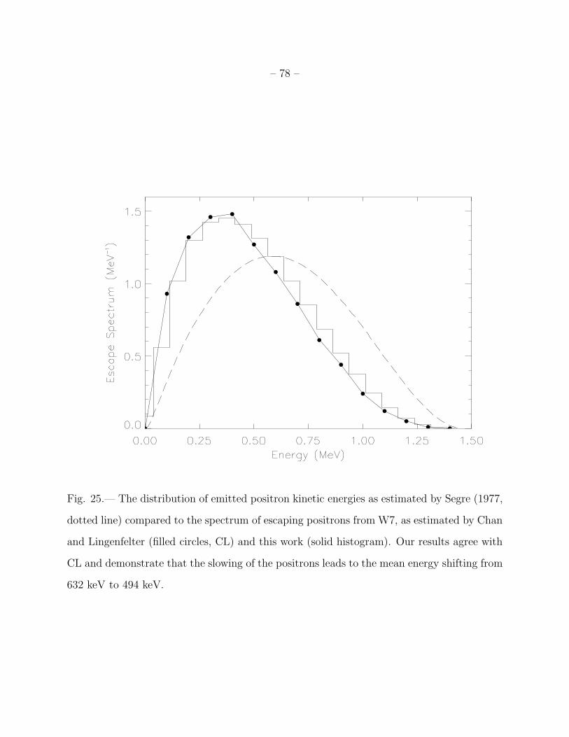
– 78 –

Fig. 25.— The distribution of emitted positron kinetic energies as estimated by Segre (1977,

dotted line) compared to the spectrum of escaping positrons from W7, as estimated by Chan

and Lingenfelter (filled circles, CL) and this work (solid histogram). Our results agree with

CL and demonstrate that the slowing of the positrons leads to the mean energy shifting from

632 keV to 494 keV.