POTENTIAL FOR SITE SPECIFIC

MANAGEMENT OF Lolium rigidum (annual ryegrass)

IN SOUTHERN AUSTRALIA

Samuel P Trengove

Thesis submitted for the degree

of

Master of Agricultural Science

In the

Faculty of Sciences

School of Agriculture, Food and Wine

Discipline of Plant and Pest Science

The University of Adelaide

9 December, 2013

2

Contents

Abstract ................................................................................................................... 5

Declaration .............................................................................................................. 8

Acknowledgements ................................................................................................. 9

1 Literature Review ........................................................................................... 11

1.1 Australian agricultural trends .................................................................... 11

1.2 Australian weed issues ............................................................................ 16

1.2.1 Cost of weeds .................................................................................... 16

1.2.2 Annual Ryegrass (Lolium rigidum) ..................................................... 17

1.3 Temporal and Spatial Population Dynamics of Weeds ............................ 26

1.3.1 Spatial distribution of weeds .............................................................. 26

1.3.2 Patch stability .................................................................................... 27

1.4 Decision Making for Variable Rate Herbicide Applications ....................... 32

1.4.1 Crop competition with weeds ............................................................. 32

1.4.2 Herbicide dose response ................................................................... 33

1.4.3 Economic thresholds ......................................................................... 34

1.4.4 Models ............................................................................................... 35

1.5 Benefits of Precision Weed Management ................................................ 37

1.5.1 Herbicide savings .............................................................................. 37

1.5.2 Improved weed control ...................................................................... 39

1.5.3 Reduced phytotoxicity effects on crops ............................................. 41

1.5.4 Herbicide efficacy targeted to soil conditions ..................................... 42

1.5.5 Environmental and food safety concerns ........................................... 43

1.6 Patch Detection Methods ......................................................................... 44

1.6.1 Manual detection ............................................................................... 44

3

1.6.2 Spectral reflectance techniques......................................................... 45

1.6.3 Machine vision ................................................................................... 51

1.6.4 Chlorophyll fluorescence ................................................................... 56

1.7 Resolution, Interpolation and Map Production ......................................... 58

1.8 Research Aims ......................................................................................... 63

2 Mapping Lolium rigidum Patches Using Spectral Reflectance Sensors ......... 64

2.1 Introduction .............................................................................................. 64

2.2 Materials and Methods ............................................................................. 65

2.2.1 Stationary sensor measurement ........................................................ 67

2.2.2 Replicated plot trial in wheat .............................................................. 76

2.2.3 Paddock scale sensor measurements with point assessments ......... 77

2.2.4 Aerial imagery from unmanned aerial vehicle (UAV) ......................... 81

2.3 Results ..................................................................................................... 82

2.3.1 Stationary sensor measurements ...................................................... 82

2.3.2 Replicated plot trial in wheat ............................................................ 105

2.3.3 Paddock scale sensor measurements with point assessments ....... 107

2.3.4 Aerial imagery from unmanned aerial vehicle (UAV) ....................... 111

2.4 Discussion .............................................................................................. 114

3 Patch Stability in Lolium rigidum Populations ............................................... 123

3.1 Introduction ............................................................................................ 123

3.2 Materials and Methods ........................................................................... 124

3.3 Results ................................................................................................... 130

3.4 Discussion .............................................................................................. 136

4 Post Emergence Herbicide Efficacy Dependence on Lolium rigidum Density

140

4.1 Introduction ............................................................................................ 140

4

4.2 Methodology .......................................................................................... 140

4.3 Results ................................................................................................... 142

4.4 Discussion .............................................................................................. 146

5 Herbicide Treatment Options for Patch Management of Lolium rigidum and

their Economic Implications................................................................................. 148

5.1 Introduction ............................................................................................ 148

5.2 Methodology .......................................................................................... 149

5.2.1 Post emergence herbicide trials in lentils ........................................ 149

5.2.2 Pre-emergence herbicide trials in wheat ......................................... 153

5.3 Results ................................................................................................... 156

5.3.1 Post emergence herbicide trials in lentils ........................................ 156

5.3.2 Pre-emergent herbicide trials in wheat ............................................ 160

5.4 Discussion .............................................................................................. 175

6 Conclusions ................................................................................................. 183

6.1 Mapping Lolium rigidum Patches Using Spectral Reflectance Sensors . 183

6.2 Patch Stability in Lolium rigidum Populations ......................................... 185

6.3 Post Emergent Herbicide Efficacy Dependence on Lolium rigidum Density

186

6.4 Herbicide Treatment Options for Patch Management of Lolium rigidum 186

6.5 Future Research Directions ................................................................... 187

7 References ................................................................................................... 188

5

Abstract

Weed spatial distribution is typically patchy and Lolium rigidum (annual ryegrass)

distribution is no exception. The potential for site specific management of annual

ryegrass was assessed to increase farmers’ financial returns through reduced

herbicide costs while maintaining weed control in commercial paddocks near Bute

and Tarlee, SA. Commercially available sensors N-Sensor, Greenseeker, Crop

Circle and digital RGB camera were assessed for their ability to detect annual

ryegrass patches in growing lentil, pea, canola and wheat crops at various growth

stages. The best platform for annual ryegrass detection was the digital camera

with an Excess Red – Excess Green algorithm applied to the image to delineate

plant matter from background soil. The best relationship for this system was an R2

of 0.85 and 0.86 in Ronnies and Stones North paddock respectively when the

lentils and peas were at the 10-12 node stage and the annual ryegrass was at

early-mid tillering.

The N-Sensor was used to map annual ryegrass in lentil, pea and canola crops

with R2 values from 0.15 to 0.88. Poor correlations were related to

misclassification due to the presence of other weed species or variability in crop

growth. When these effects were accounted for, the correlations improved with R2

from 0.27 to 0.86.

Four paddocks were monitored in three seasons between 2006 and 2009 to

determine stability of annual ryegrass populations at fixed locations. Annual

ryegrass populations were relatively stable with high density locations typically

staying high between seasons and low density locations typically staying low. The

6

relationships between seasons ranged from R2 0.53 to 0.94. Of the locations that

changed ranking from being relatively low density to relatively high between

seasons many could be explained by their proximity to the patch boundary.

Herbicide efficacy dependence on population density was assessed by counting a

wide range of annual ryegrass densities and recounting the surviving plants after

the application of herbicide. It was found that efficacy of clethodim, imazapic and

imazapyr was independent of annual ryegrass density between zero and 1600,

2000 and 6000 annual ryegrass plants m-2 in three respective paddocks.

However, there were more plants surviving at the high density locations, due to the

higher initial population. This greater number of survivors is likely important for

patch persistence.

Small plot herbicide trials were targeted at high and low density annual ryegrass

sites in lentils and wheat to assess the potential for variable applications of

clethodim in lentils and pre-emergence herbicides in wheat. Economic returns

from variable rate applications over a uniform application cannot exceed the cost

of the herbicide used uniformly at the maximum rate unless it causes yield loss

due to phytotoxic crop effects. The maximum herbicide saving that could be

achieved with clethodim in lentils was $5.42 ha-1 and this declined as high density

patch area increased. The value of applying pre-emergence herbicides site

specifically was much greater, reducing herbicide costs by $14.60 and $15.30 ha-1

in two paddocks where high density weed infestations affected 30 and 35% of the

paddock respectively. This is including additional application costs of $7.50 ha-1

for variable rate applications. Savings increased as high density patch area

decreased. Targeting patches reduces the risk of return from high cost treatments

7

and makes it economic to treat smaller patches, as low as an infestation level of

5.6% of the paddock. Where cheaper herbicides or nil treatments were applied to

low density sites there were no significant differences in annual ryegrass densities

in the year of application or the following year.

Site specific management of annual ryegrass has merit with pre-emergence

herbicides. The patches are able to be mapped in crop and patch stability means

the map can be used in subsequent seasons to target pre-emergence herbicides.

8

Declaration

I certify that this work contains no material which has been accepted for the award

of any other degree or diploma in my name, in any university or other tertiary

institution and, to the best of my knowledge and belief, contains no material

previously published or written by another person, except where due reference

has been made in the text. In addition, I certify that no part of this work will, in the

future, be used in a submission in my name, for any other degree or diploma in

any university or other tertiary institution without the prior approval of the

University of Adelaide and where applicable, any partner institution responsible for

the joint-award of this degree.

I give consent to this copy of my thesis, when deposited in the University Library,

being made available for loan and photocopying, subject to the provisions of the

Copyright Act 1968.

I also give permission for the digital version of my thesis to be made available on

the web, via the University’s digital research repository, the Library Search and

also through web search engines, unless permission has been granted by the

University to restrict access for a period of time.

Signed: Sam Trengove ................................. Date:

9

Acknowledgements

This thesis would not have been possible without the support and contribution of

many people. To Chris Preston my principal supervisor many thanks and

gratitude for your guidance and feedback throughout this study. Thank you for the

time dedicated to helping me finish, reviewing drafts and guidance in analysis and

interpretation of results. My deepest thanks to Allan Mayfield for first encouraging

me to embark on post graduate study, and encouraging my interest in the topic of

site specific weed management. The importance of Allan and Sue Mayfield’s

support and understanding as my full time employer while I was undertaking part

time study cannot be overstated, not only with my study but also with the

opportunities for me to travel and learn from others during this time. As my

supervisor Allan’s guidance and drive were motivational, particularly in the early

years of field work, and I thank Allan for continually pushing me to finish. John

Heap has been a terrific sounding board throughout this study and his ideas and

suggestions are always well considered. I have enjoyed our discussions about

new and emerging technologies and the potential for these technologies and the

findings herein to have application in the field. Many thanks John!

Thank you to Mark and Nola Branson, Max, Ros, Bill and Michelle Trengove and

Jamie Smith, the farmers that allowed me to conduct trials on their properties,

hopefully without too much disruption of your day to day activities.

Many thanks go to Stuart Sherriff for your assistance in the field. Together we

counted 65,790 ryegrass plants, 48,104 wheat plants, 32,672 ryegrass heads,

10

6,169 wild oat plants, 1,326 wild oat heads, 665 snail medic plants and a handful

of brome grass, lentil, pea and canola plants. Your good company and sense of

humour mean these tasks that might be considered repetitive and boring are

remembered with a sense of enjoyment.

Thank you to Mum and Dad for your love and support during this time, including

helping me peg trials, do plant counts and finding a lost clipboard. Thanks Ben

and Lauren for opening your home (and fridge) to me when I needed a base in

Adelaide in the early years. Finally, thanks Veronica for your love and support in

the latter years, your understanding is always appreciated!

11

1 Literature Review

1.1 Australian agricultural trends

Australian agriculture has experienced declining terms of trade over a long period

of time (ABARE 2008a). Strong global commodity prices in 2007/08 prompted

ABARE to forecast improved terms of trade for 2008-09 (ABARE 2008a).

However, rising costs of inputs and a fall in commodity prices have now caused

terms of trade to decline further (Table 1.1.1, ABARE 2008b).

Australian farmers have been forced by declining terms of trade to increase farm

scale, increase yields and improve production efficiencies to maintain

economically sustainable businesses. Figures from ABARE (2008c) show that

cropped land area per farm increased by 24 – 84% across all southern Australian

states in the 10 years from 1997 (Table 2). This can be attributed to increasing

farm sizes over this period and also to a reduction in sheep numbers in the wheat

– sheep zone. The Australia-wide five year outlook to 2012-13 is for the area sown

to grains and oilseeds to average 23.6 million hectares compared with the

previous five year average of 22.2 million hectares (ABARE 2008a).

Between 1977-78 and 2005-06, productivity growth by broadacre croppers in

Australia averaged 2.3% per year (ABARE 2008). This productivity growth has

been attributed to no-till farming techniques, improved farm management, crop

rotations, better pest and weed control methods, efficient herbicide use, advances

in tractor and machinery design and advances in plant breeding (Knopke et al.

2000; Kokic et al. 2006). However growth in productivity appears to have slowed

12

since the mid 1990’s. Between 1977-78 and 1993-94 the cropping sector

experienced average annual growth of 4.1%, compared with 0.9% between 1994-

95 and 2005-06 (ABARE 2008a). Declining productivity growth may be influenced

by external factors beyond farmers’ control, such as drought. However, Kokic et al.

(2006) report that productivity growth may still be declining even after differences

in moisture availability are taken into account.

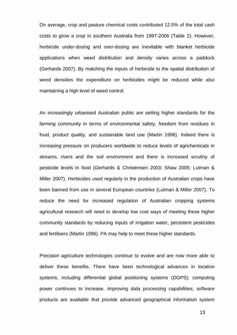
Data from ABARE (2008c) shows that total cash costs and expenditure on crop

and pasture chemicals on a per hectare basis has in many cases remained at

similar levels or declined in the 10 year period from 1997 (Table 1.1.2). This

highlights the efficiency gains made by farmers over this period in the use of crop

inputs; given that Table 1.1.1 shows that relative costs for all farm inputs have

increased over the same period. Despite this, farm cash income and rate of return

that farmers achieved were highly erratic depending on the cropping season.

During this period the value of land increased by 21 – 54%, depending on the

state.

Given the continuing rise in input costs and declining terms of trade the challenge

for farmers to stay viable is to continue to increase yields while improving the

efficiency with which inputs are used. Precision agriculture (PA) may help to

achieve these outcomes by recognising, and tailoring management decisions to,

the underlying soil variability, topography and other landscape characteristics that

underpin Australian agriculture. The promise of PA technology is to increase

production efficiency by capitalising on this spatial variability. PA is the use of

technologies that sense and consequently facilitate management of within-field

variation (Brennan et al. 2007).

13

On average, crop and pasture chemical costs contributed 12.5% of the total cash

costs to grow a crop in southern Australia from 1997-2006 (Table 2). However,

herbicide under-dosing and over-dosing are inevitable with blanket herbicide

applications when weed distribution and density varies across a paddock

(Gerhards 2007). By matching the inputs of herbicide to the spatial distribution of

weed densities the expenditure on herbicides might be reduced while also

maintaining a high level of weed control.

An increasingly urbanised Australian public are setting higher standards for the

farming community in terms of environmental safety, freedom from residues in

food, product quality, and sustainable land use (Martin 1996). Indeed there is

increasing pressure on producers worldwide to reduce levels of agrichemicals in

streams, rivers and the soil environment and there is increased scrutiny of

pesticide levels in food (Gerhards & Christensen 2003; Shaw 2005; Lutman &

Miller 2007). Herbicides used regularly in the production of Australian crops have

been banned from use in several European countries (Lutman & Miller 2007). To

reduce the need for increased regulation of Australian cropping systems

agricultural research will need to develop low cost ways of meeting these higher

community standards by reducing inputs of irrigation water, persistent pesticides

and fertilisers (Martin 1996). PA may help to meet these higher standards.

Precision agriculture technologies continue to evolve and are now more able to

deliver these benefits. There have been technological advances in location

systems, including differential global positioning systems (DGPS); computing

power continues to increase, improving data processing capabilities; software

products are available that provide advanced geographical information system

14

(GIS) features for more powerful data analysis and extraction; sensor systems for

gathering data are now more readily available; widespread availability of

broadband internet provides rapid delivery of information to end users; and the

cost of components for both hardware and software are decreasing (Rew &

Cousens 2001; Jurado-Expósito et al. 2003; Shaw 2005).

Table 1.1.1: Indexes of prices received and paid by farmers, and terms of trade from 2002-03 to 2008-09 (ABARE 2008b).

2002-03 2003-04 2004-05 2005-06 2006-07 2007-08 2008-09f

Farmers' terms of trade 101.0 95.0 91.7 91.0 94.1 92.6 87.5

Prices received by farmers

Barley 159.9 105.9 100.1 93.9 153.3 167.7 135.8

Canola 100.9 104.4 84.5 86.5 102.8 136.8 123.1

Cotton 100.1 88.2 87.0 85.0 86.2 93.6 97.1

Hay 155.0 125.0 128.0 143.7 151.8 165.1 173.4

Lupins 149.0 120.4 105.2 99.8 135.8 137.1 123.4

Oats 160.3 101.1 98.1 107.8 176.6 148.5 143.7

Sorghum 120.9 93.8 79.4 84.6 126.1 111.6 108.2

Wheat 134.4 109.1 99.6 102.5 122.4 200.2 186.6

Prices paid by farmers

Capital items 118.3 121.3 124.4 128.4 132.3 136.8 141.5

Chemicals 108.0 110.0 111.9 114.6 124.7 149.7 172.1

Fertiliser 106.9 102.8 108.8 111.6 121.4 220.4 264.5

Fuels and lubricants 127.0 144.3 167.2 210.6 208.3 243.7 300.2

Insurance 124.5 128.8 131.9 135.1 139.4 143.5 148.4

Interest paid 110.7 118.1 120.9 123.8 127.8 131.5 136.0

Labor 117.9 121.6 125.7 129.7 133.5 138.0 142.9

Marketing 115.9 118.7 121.5 125.4 129.1 133.5 138.1

Rates and taxes 119.1 121.9 124.8 128.9 132.7 137.3 142.0

Seed, seedlings and plants 118.3 104.9 95.3 93.8 109.5 130.9 127.5

Total prices paid 121.5 123.0 126.3 129.4 135.8 151.6 160.2

f ABARE forecast. The indexes for commodity groups are calculated on a chained weight basis using Fisher’s ideal index with a reference year of 1997-98 = 100.

15

Table 1.1.2: Broadacre crop farm statistics for the 10 year period from 1997 to 2006 (ABARE 2008c).

State YearTotal area

cropped (ha)Index

Crop and pasture

chemicals ($/ha)Index

Total cash

costs ($/ha)Index

Value of land and fixed

improvements ($/ha)Index

Farm cash

income

($/ha)

Index

Rate of return

excluding capital

appreciation (%)

New South Wales 1997 622 100 58 100 665 100 2404 100 226 100 7New South Wales 1998 576 93 51 87 663 100 3174 132 274 121 5New South Wales 1999 738 119 54 93 553 83 2313 96 231 102 7New South Wales 2000 722 116 71 122 618 93 2511 104 169 75 2New South Wales 2001 712 114 66 113 607 91 2314 96 200 88 4New South Wales 2002 760 122 56 96 567 85 2212 92 274 121 7New South Wales 2003 630 101 38 65 447 67 3380 141 174 77 2New South Wales 2004 761 122 52 88 481 72 4134 172 77 34 2New South Wales 2005 867 139 39 66 390 59 2974 124 96 42 2New South Wales 2006 1038 167 50 85 497 75 2902 121 188 83 4Victoria 1997 608 100 38 100 392 100 1518 100 204 100 7Victoria 1998 616 101 39 103 372 95 1736 114 117 57 -1Victoria 1999 688 113 38 101 303 77 1821 120 96 47 -1Victoria 2000 642 106 53 142 385 98 1928 127 160 79 3Victoria 2001 590 97 45 119 410 105 1944 128 241 118 7Victoria 2002 707 116 41 110 372 95 1940 128 290 142 8Victoria 2003 806 133 32 84 270 69 1924 127 79 39 -2Victoria 2004 833 137 44 117 294 75 2103 139 140 69 4Victoria 2005 839 138 45 120 315 80 2066 136 72 36 0Victoria 2006 917 151 43 114 341 87 2127 140 67 33 1South Australia 1997 516 100 45 100 390 100 1807 100 185 100 5South Australia 1998 679 132 49 108 373 96 1731 96 206 111 5South Australia 1999 677 131 44 97 338 86 1679 93 137 74 2South Australia 2000 657 127 41 92 318 81 1640 91 135 73 0South Australia 2001 784 152 35 78 339 87 1598 88 217 117 7South Australia 2002 736 143 48 107 399 102 1927 107 296 160 9South Australia 2003 878 170 59 130 347 89 2531 140 217 118 4South Australia 2004 862 167 46 102 324 83 2762 153 207 112 3South Australia 2005 881 171 38 84 298 76 2733 151 103 56 1South Australia 2006 950 184 45 100 364 93 2778 154 79 43 1Western Australia 1997 1771 100 56 100 347 100 1039 100 113 100 6Western Australia 1998 1674 95 53 96 345 99 1101 106 150 133 7Western Australia 1999 1812 102 53 95 334 96 1185 114 84 75 3Western Australia 2000 1584 89 44 78 322 93 1151 111 98 87 3Western Australia 2001 1701 96 39 69 283 81 1123 108 27 24 -1Western Australia 2002 1745 99 38 69 318 92 1114 107 96 85 5Western Australia 2003 1930 109 43 77 289 83 1311 126 57 50 1Western Australia 2004 1806 102 45 80 289 83 1309 126 137 121 7Western Australia 2005 2191 124 51 91 337 97 1644 158 102 90 4Western Australia 2006 2204 124 48 86 303 87 1524 147 52 46 1

16

1.2 Australian weed issues

1.2.1 Cost of weeds

Weeds are a major cost to Australian cropping systems. The 15 most important

weeds of seven winter crops in Australia were estimated to cost A$1182 million in

1998-99, which resulted in a loss in economic surplus of A$1,278.9 million,

representing 17% of the total value of Australia’s grain and oilseed production of

A$7,038 million for 1998-99. The main components of this cost were herbicides

(A$571 million), competitive effects of residual weeds (A$380 million) and tillage

(A$206 million) (Jones et al. 2005). This is a similar result to estimates by

Combellack (1987) of a total annual financial cost of A$1,271 million, consisting of

A$592 million for tillage costs and A$171 million for herbicides. The large

discrepancy in herbicide and tillage costs between the two studies can be

explained by the increased adoption of no-till farming practices over the 10 year

period between the studies, resulting in greater reliance on herbicides for weed

control and less use of tillage in 1998-99. The study by Combellack (1987) also

included a wider range of crops. It is expected that the adoption of no-till has

continued to increase in the time since the year of study by Jones et al. (2005) and

that the herbicide component has continued to increase and the tillage component

reduced further. Jones et al. (2005) report that annual ryegrass (Lolium rigidum),

wild oats (Avena fatua) and wild radish (Raphinus raphinistrum) were the most

economically important weeds across all regions.

17

1.2.2 Annual Ryegrass (Lolium rigidum)

1.2.2.1 Background and ecology

The genus Lolium was made reference to in Australia as early as 1798, when

‘drake’ was reported as a weed of wheat in New South Wales. The genus Lolium

consists of 8 species, which are native to Europe, temperate Asia, North Africa

and the North Atlantic islands. Three of these species are wind-pollinated

outcrossers, including L. rigidum, L. perenne and L. multiflorum, the remainder are

self pollinated. Crossbreeding between the outcrossing species produces a wide

range of fertile hybrids that continue crossing and backcrossing to produce near

continual variation in every character (Kloot 1983). L. rigidum is the most

widespread ryegrass in Australia, being present in all states. It was cultivated

widely as a pasture plant; however by 1980 it was reported as the major grass

weed of field crops in southern Australia (Kloot, 1983).

Kloot (1983) provides the following description of L. rigidum: “Annual to 120 cm;

stems reddish even at maturity; leaf blades to 20 cm X 8 mm, acute, glabrous

beneath, glabrous or (occasionally) scabridulous above, generally shiny in

appearance; spike 3-30 cm; rachis flexuose, slender to somewhat rigid, to 1.8 mm

diameter; spikelets 4-1 8 X 2-5 mm with 3-11 fertile and 0-2 rudimentary florets;

glumes lanceolate or narrowly oblong, about the same length as the spikelet;

lemma unawned or occasionally with an awn to 3 mm.” Hereafter, unless

otherwise indicated, annual ryegrass refers to L. rigidum.

Annual ryegrass is now recognised as one of the most troublesome weeds of

cereals grown in Mediterranean climates and is now an important weed of

18

Australia, France, Iraq, Portugal, Spain and Argentina (Gill 1996). Annual ryegrass

can cause up to 80% yield loss in wheat depending on seasonal conditions and

density (Gonzalez-Andujar & Fernandez-Quintanilla 2004).

There are a number of characteristics that contribute to the weediness of annual

ryegrass in southern Australian cropping systems, including:

High genetic variability: contributes to its ability to adapt to a wide range of

climate and soil conditions (Gill 1996a).

Large seed production: annual ryegrass can produce large numbers of

seed with the potential to produce over 1000 seeds per plant (Reeves & Smith

1975). Production of 31 000-45 000 seeds m-2 has been reported in a wheat crop

under irrigated conditions (Rerkasem et al. 1980).

High plasticity: annual ryegrass has a great ability to tiller to utilise available

space and resources (Gill 1996a).

High seed survival over summer and autumn: short-lived innate dormancy

prevents germination with sporadic summer rainfall events and temperature is the

major regulator of dormancy (Steadman et al. 2003). Between 40-80% of seeds

germinate at the break of the season when plant establishment and survival are

favoured. In addition to this, Gramshaw (1976) reports that potential seed

germination rate is increased whenever seeds are wetted substantially, thus

summer rains will affect seedling recruitment in autumn.

Staggered germination: annual ryegrass can germinate in several cohorts

throughout the growing season. Gramshaw (1972) showed that almost total

germination of the seed bank can occur within 4-6 days under non-limiting

moisture conditions, with temperatures cycling between 12 and 24ºC and

exposure to light for 12 hours a day. However meteorological data for many

19

southern Australian localities indicates that autumn rain is rarely continuous for

more than 2-3 days. Later cohorts are less important for crop competition and yield

loss but contribute to seed bank persistence by avoiding control and producing

seed.

Dark dormancy: 10-20% of the seed population can exhibit dark dormancy

(Gramshaw & Stern 1977b), whereas seed in light conditions at the soil surface do

not exhibit this dormancy characteristic. This component of the seed bank slowly

loses its dormancy and progressively germinates with shallow burial. This may be

important for short term persistence of the seed bank. However, the non-dark

dormant component of the ryegrass seedbank tends to have a higher rate of

germination under dark conditions than light conditions (Gramshaw 1976), thus

cultivation and subsequent burial of seeds may increase germination rates of the

non-dark dormant component.

Crop-weed competition: annual ryegrass can compete with wheat as early

as the two leaf stage in heavy infestations and cause significant yield loss in a

wide range of crops (Gill 1996a).

Climate suitability: annual ryegrass is native to regions with temperate

climatic conditions, similar to those found in southern Australia (Gill 1996a).

Deliberate introduction over a large area: annual ryegrass was

recommended for sowing in pastures in most areas of southern Australia (Gill

1996a).

Relatively infertile soils with open crop canopies: low fertility Australian soils

produce crops with less early vigour that allow weeds to establish and reproduce

successfully in the crop (Gill 1996a).

Frequent replenishment: of the seed bank: total prevention of seed

production is rare in Australia (Gill 1996a).

20

Short growing season: using all of the available growing season for crop

growth is important for maximising crop grain yield; therefore there is a conflict

between sowing crops early for maximum crop yield and delaying sowing to

maximise germination of the weed seed bank for pre-seeding weed control. As a

result, substantial germination takes place with, or soon after crop establishment

(Gill 1996a; Gill 1996b).

Annual ryegrass characteristics have implications for how it responds to changing

Australian farming systems, with increasing adoption of minimum and no till

farming practices (Llewellyn et al. 2004). In more conventional farming systems

the autumn ‘tickle’ is a strategy that has been used by farmers to stimulate annual

ryegrass germination prior to sowing. A tickle is a shallow cultivation used to bury

the seed to increase germination. In reduced tillage farming systems this is no

longer practiced, with crops sown into undisturbed crop stubbles from the previous

year. Chauhan et al. (2006a) showed that seedling recruitment of ryegrass was

lower under low soil disturbance disc tillage systems than under high soil

disturbance tine tillage systems. Lower seedling recruitment under the low

disturbance system was attributed to leaving more seed on the soil surface, where

it is prone to rapid desiccation and more susceptible to insect predation.

Conversely in the high disturbance systems the seed was adequately covered with

soil and more favourable conditions of moisture and temperature increased

seedling recruitment. In addition, the lower disturbance systems had slower

seedling recruitment of ryegrass and the size of the plants was smaller, reducing

its competitive ability. Although the level of disturbance from tillage had large

effects on seedling recruitment, it was found to have little effect on seed bank

persistence, due to a compensatory effect of greater decay of seed in the low

21

disturbance systems with more seed left at the soil surface. Greater decay at the

soil surface may be caused by exposure to greater fluctuations in environmental

conditions that cause metabolic failure, greater loss through predation by insects,

and increased mortality caused by germination in unfavourable conditions

(Chauhan et al. 2006b). However, it was found that dinitroaniline herbicides had

greater efficacy on ryegrass when incorporated by sowing with the higher

disturbance tine systems compared to the low disturbance disc systems. This may

be attributed to greater soil coverage of the herbicides in the inter-row space,

reducing herbicide losses due to volatilisation and photodecomposition and

increasing the duration of efficacy on weeds (Chauhan et al. 2007).

1.2.2.2 Chemical and cultural control

Selective removal of annual ryegrass from some commonly grown crops with

effective herbicides became available in 1973 with the release of the pre-

emergence herbicide trifluralin. In 1978 diclofop-methyl was released for use and

other aryloxyphenoxypropionate herbicides such as fluazifop, haloxyfop and

quizalofop followed. Chlorsulfuron was the first acetolactate synthase (ALS)

inhibiting herbicide used from 1982 and was rapidly adopted for its ability to control

annual ryegrass and a wide range of dicotyledonous weeds in wheat (Llewellyn &

Powles 2001; Owen et al. 2007). The cyclohexanedione herbicide sethoxydim was

released in 1986 and other chemicals from the same group have been released

and recommended for annual ryegrass control (Matthews 1996c). In 1996 seven

herbicides were registered for the selective control of annual ryegrass in wheat,

yet sales indicate that two dominated the market. Additional herbicides were

available for selective control in broadleaf crops, but the market was again

22

dominated by only a few of these from the same chemical and mode of action

groups as the cereal selective herbicides (Matthews 1996b).

Llewellyn et al. (2004) reported that grain growers perceive herbicide-based weed

control practices as the most cost-effective, and as a result herbicides are the

most used weed control tactic. Yet the application of selective herbicides to annual

ryegrass has seen the development of many populations with herbicide resistance

(Matthews 1996b). However, there are a number of cultural control tactics that can

be used in an integrated weed management system to improve ryegrass control.

Some of these include pasture and pulse spray topping, stubble burning, seed

catching, cultivation, increased seeding rates, competitive crop species or

cultivars, delayed sowing, green manuring, harvesting low and burning windrows,

cutting hay and heavy grazing. Management systems that integrate various control

options are likely to minimise the size of the seed bank and provide the best long

term benefits (Matthews 1996a; Gonzalez-Andujar & Fernandez-Quintanilla 2004;

Llewellyn et al. 2004).

Grazing of annual ryegrass seed heads by sheep or cattle to reduce seed

returning to the seedbank relies on the ingested ryegrass seed being destroyed in

the digestive system of the animal. However, Gramshaw and Stern (1977a) found

that grazing standing ryegrass heads only removed 20% of seed from being

returned to the seedbank. Grazing during the spring and summer resulted in about

70% of mature seed falling to the ground, while sheep consumed part of the 30%

that remained in the seed heads. The use of chaff carts for seed catching at

harvest also results in large amounts of chaff that need to be removed from the

paddock. This is done by either burning or by feeding to livestock. Matthews

23

(1996c) reported the number of seeds removed in the seed catching process can

range from 5 to 81% of pre harvest density. This variability depends on the cutting

height of the crop, the crop type and the period of time between ryegrass maturity

and crop harvesting. Crop type itself affects the cutting height of the crop, time of

harvest relative to ryegrass maturity and the level of vigour with which the material

is threshed. More vigorous threshing results in more seed being separated from

the rachis, therefore ending up in the chaff cart. In a study by Stanton et al. (2002)

it was found that 10.8 and 32.8% of seed ingested was excreted by sheep and

cattle respectively, with 3.9 and 11.9% of the seed ingested remaining germinable

for sheep and cattle. Annual ryegrass seed was present in the faeces of both

sheep and cattle within 24 hours of ingestion, and continued to be excreted five

days after removal from the diet. This has implications for the dispersal of seed to

clean paddocks or properties and also for the dispersal of seed around a paddock.

1.2.2.3 Herbicide resistance

Weed species are genetically variable and this diversity allows the selection of

traits that enable them to cope with pressures imposed by the environment. The

repeated use of herbicides for weed control is probably the greatest selection

pressure imposed on weeds (Gill 1995). Herbicide resistance in annual ryegrass

in Australia was first confirmed with diclofop-methyl, only four years after its’

commercial release for use by growers (Heap & Knight 1982). A study by Gill

(1995) on annual ryegrass samples from the Western Australian wheat belt

reported that resistance was present in all samples that received seven or more

applications of aryloxyphenoxypropionate (‘fops’) and cyclohexanedione (‘dims’)

(Group A) herbicides or four or more applications of sulfonylurea (SU; Group B)

24

herbicides. For the period from 1991 to 2004 a total of 3090 annual ryegrass

samples from across the southern Australian wheat belt were tested for resistance

to a range of herbicides. It was found that 77% of samples were resistant to Group

A fop herbicides, 40% resistant to Group B, 22% resistant to Group A dim

herbicides, 8% resistant to trifluralin (Group D), 1% resistant to triazines (Group C)

and 0.4% resistant to glyphosate (Group M) (Broster & Pratley 2006). However,

these samples were not collected randomly and may be biased towards

individuals that were exhibiting herbicide resistance, i.e. they were sampled and

tested because they had survived a herbicide application. Annual ryegrass

samples taken from 215 random paddocks across South Australia in 1998 showed

that 38% were resistant to Group A, 21% resistant to Group B and 6% with

resistance to both Group A and B herbicides (McGillon & Storrie, 2006). In 2003

this was repeated with samples taken from 170 random paddocks, this time the

resistance levels had increased to 76, 75 and 59% for Group A, Group B and

Group A and B respectively (McGillon & Storrie 2006). Similar results were found

in Western Australia, where a survey conducted in 1998 found that 46% of

samples were classified as resistant or developing resistance to the Group A

diclofop-methyl, this had increased to 68% by 2003 (Owen et al. 2007).

Resistance to the Group B sulfonylureas had also increased from 64 to 88% over

the same time period (Owen et al. 2007). There are large differences in resistance

to different chemical groups between states, and agronomic regions within states.

This is highlighted at state level with WA and NSW having the highest proportion

(26%) of samples resistant to Group A dims compared with SA (14%), and also

WA had the highest level of Group B resistance (61%) followed by NSW (44%),

SA (30%) and Vic (25%) (Broster & Pratley 2006). Regionally this is highlighted by

annual ryegrass resistance to trifluralin in SA. In 2003 84% of samples collected

25

from the Yorke Peninsula exhibited moderate levels of resistance compared with

44% from the Lower North and 19% in the Mid North (Boutsalis and Preston

2012). Regional differences are caused by different cropping and herbicide use

history. The influence of soil types and of local agronomists may also be important

(Llewellyn & Powles 2001; Broster & Pratley 2006).

The cost of herbicide resistance can be placed into two categories; one is to

replace the herbicide to which resistance has developed with an alternative

method of weed control and the other is the cost of yield reductions that may result

from higher weed densities due to poorer weed control (Llewellyn & Powles 2001).

In a random survey of herbicide resistance in annual ryegrass from 264 cropping

fields in Western Australia in1998 it was found that there was no correlation

between the levels of resistance to diclofop-methyl and chlorsulfuron and weed

density. This may be due to the availability of cost effective alternative annual

ryegrass control options at that time to maintain low ryegrass densities (Llewellyn

& Powles 2001). Pannell et al. (2004) show that loss of herbicides due to herbicide

resistance has large economic effects, because as herbicide options are lost from

the system alternative weed control systems are introduced that are approximately

as effective as herbicide based systems, but at higher cost. Annual ryegrass

continues to develop resistance and multiple resistances to a range of herbicides

and for this reason is considered among the most important examples of economic

disruption due to herbicide resistance in world agriculture (Broster & Pratley 2006).

26

1.3 Temporal and Spatial Population Dynamics of Weeds

1.3.1 Spatial distribution of weeds

Most weed management practices are applied uniformly across fields, yet many

agronomically important weeds are spatially aggregated in distribution (Lutman &

Miller 2007). Some studies differentiate between weed aggregations and patches

based on a temporal condition. Krohmann et al. (2006) describe a weed

aggregation as weedy areas in one year, whose distance from each other does

not exceed a maximum distance. Weed patches were defined as areas where

weeds appeared in four of the five years of their study at the same location

(Krohmann et al. 2006). Wilson and Brain (1991) defined weed patches as

populations of the same weed species that occur at the same position in more

than 50% of the years of a study period. However, most other studies do not

appear to include a temporal condition in their definition of a weed patch. Backes

and Plümer (2005) describe the spatial characteristics of shapes by geometrical

parameters such as the centre of gravity, the area, the perimeter and the

compactness of the patch.

A number of reasons are likely to explain why weeds appear patchy. Field habitats

may be patchy, for example in soil type, slope and crop competition, with particular

species more abundant in their preferred habitat; weed mortality may be patchy,

perhaps due to uneven spraying or herbicide interactions with soil properties

causing variable efficacy; dispersal may be highly aggregated, due to harvester

swathing or from ants collecting seeds around nests for example; the weed may

27

still be invading and has not spread to all parts of the field yet (Cousens &

Woolcock 1997; Dieleman et al. 2000; Williams et al. 2001).

Identifying relationships between particular weed species and site properties

would reduce the sampling time and costs in weed map production (Rew &

Cousens 2001) and relationships between soil properties and weed species have

been demonstrated with good correlations in a number of studies (Dieleman et al.

2000; Walter et al. 2002). However, the relationships tend to be specific for each

year, field and species, therefore making the prediction of weed occurrence for

SSWM difficult based on site properties (Medlin et al. 2001; Rew & Cousens 2001;

Walter et al. 2002).

Seed bank and seedling density varies within patches, generally characterised by

high density patch centres and low density patch edges (Mortensen & Dieleman

1997).

1.3.2 Patch stability

The stability of patches is important, as it impacts on how long a map will suitably

explain the spatial distribution of a weed population and therefore the frequency of

mapping required to maintain an accurate map. The cost of mapping is significant

for the overall profitability of patch spraying and therefore mapping frequency will

have a significant impact (Goudy et al. 2001; Lutman & Miller 2007). To assess

patch stability, correlations between weed infestation data at specific locations and

times has been used. A review of the literature by Lutman and Miller (2007) shows

that these correlations are much less than 1.0, with the studies reported showing

28

R2 correlations ranging from 0.15 to 0.46. Rew et al. (2001) report correlation

coefficients from three consecutive years 1997-1999 with a range of 0.369 to

0.784, the highest correlation being obtained between years 1997 and 1999.

Flaws in using correlation techniques for year to year comparisons can partly

explain these low correlations. For example, if weeds are more abundant in one

year than another then the patch appears to expand, and although the patch has

not moved the correlations will be poor (Lutman & Miller 2007).

Several studies have found that the patch centres of weeds tend to be stable over

time; however significant fluctuations in patch boundary location and weed

densities between seasons are more common (Cardina et al. 1997; Mortensen &

Dieleman 1997; Dieleman & Mortensen 1999; Rew & Cousens 2001).

Variability in patch size and density can often be associated with localised

conditions for seedling recruitment. Cardina et al. (1997) counted emergence of

weeds in a no-till soybean field repeatedly over a six week period and found that

the spatial pattern of emergence was not uniform over time, suggesting that sites

favouring emergence were not constant. This was associated with differential

warming of various parts of the field due to soil colour, aspect and residue cover.

Zanin et al. (1998) report safe sites as a zone that provides: (1) stimuli for

dormancy breaking, (2) conditions for germination to proceed, (3) availability of

resources for growth and (4) absence of hazards and the distribution of safe sites

is largely determined by the soil microtopography. Annual variability in weather

conditions, extent of seedbank carry-over and the effectiveness of weed control

practices also affect density stability between seasons and the movement of patch

boundaries (Dieleman & Mortensen 1999).

29

Some studies have also shown that seedling survival of pre and post-emergence

applications of herbicides increases with population density (Winkle et al. 1981;

Dieleman & Mortensen 1999), indicating that a higher mortality percentage is

required to limit weed seedling populations in high density locations. This attribute

may help explain the persistence of high density patch centres and suggests that

something other than uniform weed management will provide more effective long

term population regulation (Mortensen & Dieleman 1997).

Colbach et al. (2000) found that the level of patch persistence is most likely the

result of dispersal rate, dispersal distance and the ability of a weed to colonise,

and that in general persistence was greater for perennial weed species with low

dispersal rates than for annual weed species with high dispersal rates. These

factors have also been found to be important in affecting the level of patchiness

exhibited by a weed species (Dieleman & Mortensen 1999; Paice et al. 1998), and

density has been found to be inversely related to patchiness (Wiles & Brodahl

2004).

Variability in total seed production is expected to cause patches to expand in years

of high production and contract in years of low production (Dieleman & Mortensen

1999). Gerhards et al. (1997) found that years with high seedling density

corresponded with the largest patch sizes. The size of the seedbank is an

indication of potential weed emergence (Nordmeyer 2005); however, studies have

shown for some species that there is often considerable lack of correlation

between the seedbank and resulting weed emergence and that this relationship is

complex and dynamic (Grundy 1997). In a study on the seedling recruitment of 25

species Webster et al. (2003) found that only six were correlated with seed rain

30

from the previous autumn, spring soil seedbank samples or a combination of the

two. However, it was found that seedling recruitment of the dominant annual

grasses was related to seedbank number or a combination of seedbank and seed

rain densities. Blanco-Moreno et al. (2004) suggest that in the case of annual

ryegrass the existing seedbank is less important due to the short life of seeds in

the soil and more considerations should be given to the seed rain from the

previous season.

The pattern of weed seed dispersal and patch spread is also important in

determining the usefulness of historical weed maps for use in future seasons.

Weed populations that use a ‘phalanx spread’ strategy or spreads with a closed

advancing front can be mapped at an earlier date and potentially used for several

seasons as the patch spread is predictable. However, populations that use a

‘guerrilla spread’ strategy, where a small proportion of seeds may be moved large

but unpredictable distances to form new colonies, may require a well structured

monitoring program to detect new patches in order to maintain an accurate map

(Woolcock & Cousens 2000; Wallinga et al. 2002; Barosso et al. 2006). Combine

harvesters favour a guerrilla spread strategy (Barosso et al. 2006) and a large

proportion of annual ryegrass seed is subject to dispersal by combines as they are

retained in the seed head at the time of grain harvest. Therefore, frequent

remapping of annual ryegrass may be necessary to maintain an accurate map,

although the use of chaff carts behind combine harvesters to collect any seed that

passes through the machine may help reduce dispersal by these means.

Lutman and Miller (2007) suggest two ways for overcoming the uncertainty of

reliability of historical maps. Buffers could be added to patches to ensure that low

31

density areas around core patches are treated. Rew et al. (1997) recommend

adding a 4 metre buffer around patches to account for seed movement, navigation

errors and sprayer response times. Secondly, a basal low cost treatment can be

applied to the non-patch areas, with a higher rate or additional chemical applied to

treat patches (Lutman & Miller 2007).

32

1.4 Decision Making for Variable Rate Herbicide Applications

1.4.1 Crop competition with weeds

Competition between weeds and crops is the result of uptake of limited resources

(Lemerle et al. 2004). Studies assessing the interaction between annual ryegrass

and wheat have shown that crop density has a significant impact on the growth

and seed production of annual ryegrass. Medd et al. (1985) found that biomass

production of annual ryegrass at low densities (up to 100 plants m-2) was 100

times greater when in competition with 40 wheat plants m-2 than when in

competition with 200 wheat plants m-2. Similarly, Lemerle et al. (2004) found that

doubling wheat density from 100 to 200 plants m-2 halved the biomass production

of annual ryegrass from 100 grams m-2 to 50 grams m-2, and crop yield in the

presence of weeds increased with crop density as the crop population accessed

an increasing proportion of the available resources. Higher crop densities gave

diminishing marginal reductions in annual ryegrass biomass production. As weed

biomass is positively correlated with seed production the effects of crop

competition on weed growth will affect the replenishment of the weed seedbank.

It has been shown that crop yield loss from weed competition is over estimated

when a uniform weed distribution is assumed (Brain & Cousens 1990; Thornton et

al. 1990; Wiles et al. 1992; Cardina et al. 1997; Garrett & Dixon 1998). Weeds

growing in close proximity compete with each other and this intraspecific

competition between weeds reduces competition between weeds and the crop,

with the greatest competition between weeds and crop occurring for the

33

hypothetical situation where weeds are uniformly distributed across a field.

Therefore, yield loss decreases as patchiness increases (Wiles et al. 1992).

1.4.2 Herbicide dose response

SSWM requires the determination of the correct herbicide dose to apply to patch

and non-patch areas and implies that there is a target weed density to be achieved

through applying the herbicide, and a known dose response curve from which a

rate can be selected to achieve the desired efficacy. However, factors such as

weed size, density, age, stress, application conditions and history influence

herbicide efficacy and can make herbicide dose response difficult to predict (Thorp

& Tian 2004a). Variability in soil conditions can also influence the bioactivity of soil

applied herbicides (Blumhorst et al. 1990).

A decision algorithm for patch spraying (DAPS) has been developed in Denmark

as a decision support tool to identify the appropriate herbicide rates for patch

spraying (Christensen et al. 2003). DAPS has a database with dose response

information of herbicides for common weed species, crops, crop growth stages

and standard weather conditions in Denmark. It also incorporates a crop-weed

competition model to calculate the economically optimal herbicide dose. There is

an argument that reducing herbicide doses will result in increased uncertainty in

efficacy and poorer control (Paice et al. 1998). Christensen et al. (2003) argue that

a low herbicide dose will often retard weed growth even if not providing complete

control, and will be suppressed further by crop competition. DAPS was used in a

five year study to test the hypothesis that the benefit of using low herbicide doses

will diminish over time as weed density will increase and higher doses will be

34

required, however the results of the study did not confirm this (Christensen et al.

2003).

Manalil et al. (2011) studied the impact of using low rates of diclofop on the

evolution of herbicide resistance evolution in a diclofop susceptible population of

annual ryegrass. Their study found rapid evolution of diclofop resistance in the

selected annual ryegrass lines. In addition, there were moderate levels of

resistance in the selected lines to herbicides that the population had never been

exposed (Manalil et al. 2011). Enhanced herbicide resistance development in

annual ryegrass is likely to limit the SSWM application of a high dose/low dose

herbicide strategy in high and low density populations. However, an on/off

approach may still be appropriate, negating the development of herbicide

resistance development through the application of low rates.

1.4.3 Economic thresholds

Economic thresholds for weed control are determined based on expected yield

loss and the cost of an action to reduce the number of weeds (Garrett & Dixon

1998). Threshold density occurs where the cost of control is equal to the net

benefit of control. In this case the weed control action is the application of

herbicide. Historically, economic thresholds have been applied across whole

fields; SSWM implies that the economic thresholds are applied at the scale of the

application equipment. Economic thresholds applied at the whole field scale must

consider the cost of application in the equation, with higher cost of application

increasing the threshold density. Applying economic thresholds spatially across

fields means that the cost of application is incurred anyway, regardless of the

35

decision to treat or not, as the application equipment has to pass over the whole

field. This reduces the economic threshold for weed control.

1.4.4 Models

Models that seek to determine the economic threshold for weed control often only

consider the year of treatment and do not consider the long term ramifications of

treatment decisions, such as the addition of seed to the seedbank and the cost

involved in controlling weeds in future years (Czapar et al. 1997; Wilkerson et al.

2002). In reality this is an important consideration for growers and needs to be

accounted for by models. Growers seeking to maximise their economic return over

the long term will have lower weed thresholds for control than a grower seeking to

maximise economic return in a single year, and when considered over a very long

period the threshold may approach zero (Wallinga et al. 1999).

The resistance and integrated management (RIM) model has been developed for

annual ryegrass and represents weed and seedbank population dynamics, weed-

crop competition, weed treatment impacts, as well as agronomic and financial

details. It can account for herbicide resistance development in populations that

implies a sudden loss in efficacy (Pannell et al. 2004). Consideration of weed and

seedbank population dynamics overcomes the problem of accounting for

treatment decisions across seasons.

Models of weed and crop interactions and their effect on yield generally require

measures of weed density; however measures of percentage ground cover and

relative leaf area have been used in yield loss equations (Kropff & Spitters 1991;

36

Lotz et al. 1996; Wilkerson et al. 2002). These measurements help to account for

differences in weed emergence time relative to the crop that simple weed density

measurements do not reflect. Measurement of relative leaf area or ground cover

may become more readily available and reflect spatial variability with the

development of weed detection technology. It is unclear how measurements of

ground cover and leaf area can be used to predict long term population dynamics,

where estimates of weed seed production are required. Czapar et al. (1997) and

Wilkerson et al. (2002) cite the time and effort required to collect weed density

information as an impediment to the use of models for weed management

decisions, so weed detection technology for measurement of weed density may

result in increased use of such models.

37

1.5 Benefits of Precision Weed Management

1.5.1 Herbicide savings

The most common benefit cited for SSWM is that of herbicide savings. The

herbicide savings are generally reported as the amount of herbicide used to spray

the weed patches compared with what would have been required to treat the

paddock uniformly with a full rate. Herbicide savings tend to be greater for on/off

(spray/no spray) treatment decisions rather than high dose/low dose treatments;

however the former is considered more risky as untreated patches have the

potential for weed escapes to contribute seed to the seed bank and create

problems for future seasons (Rew et al. 1996; Lutman & Miller 2007). The savings

associated with these two approaches are influenced by the herbicide type, rates

and cost used at the maximum rate, weed biology, crop yield potential and the

dose of the low rate applied in the high dose/low dose scenario (Christensen et al.

2003). Determination of the ‘100% treatment’ can generally be made from label

recommendations; however in many cases the performance of lower rates is

uncertain. Some products have steeper dose response curves than others, and

this information in conjunction with information on the effects of surviving weeds is

required to determine the lower rates (Lutman & Miller 2007). In Denmark the

decision algorithm for patch spraying (DAPS) has been developed linking dose

response data from their decision support system PC-Plant Protection to patch

treatment (Christensen et al. 2003). However, the potential of DAPS has not really

been tested due to limited uptake in Denmark (Lutman & Miller 2007).

38

Herbicide savings are also influenced by the resolution of weed mapping, the size

and shapes of the weed patches and the resolution of the spray application

technology, therefore herbicide savings are not always directly related to the level

of weed infestation in the field (Wallinga et al. 1998; Barroso et al. 2004; Lutman &

Miller 2007). This will be discussed in more detail in Section 1.7. Herbicide savings

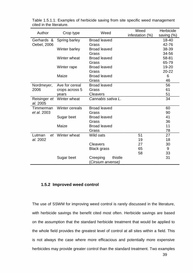
cited in the literature have ranged from as little as 6% up to 90% (Table 1.5.1.1)

often due to large differences in infestation area. Dicke and Kühbauch (2007)

report up to 100% savings for grass and broadleaved herbicides in cereals and

down to 0% savings in maize and sugar beet.

Modelling of the long term impact of on/off decisions compared with low dose/high

dose indicate that the former is likely to fail, because small patches and isolated

plants outside sprayed patches act as foci for field re-colonisation (Lutman & Miller

2007). However, a long term field study over four years by Gerhards and

Christensen (2003) found that high density Alopercus myosuroides (black grass)

patches persisted at the same locations within a field despite effective herbicide

application every year, while population density did not increase at locations below

the economic threshold where herbicides were not sprayed.

No examples of using an on/off strategy for only one herbicide in a chemical mix

were found in the literature. This strategy could allow significant savings of an

expensive herbicide in the mix while reducing the risk of escapes associated with

the on/off strategy, by applying a basal herbicide across the whole field, ensuring

some level of control for weeds outside of the identified patches.

39

Table 1.5.1.1: Examples of herbicide saving from site specific weed management cited in the literature.

Author Crop type Weed Weed

infestation (%) Herbicide saving (%)

Gerhards & Oebel, 2006

Spring barley Broad leaved 18-40 Grass 42-76 Winter barley Broad leaved 38-39

Grass 34-56 Winter wheat Broad leaved 58-81 Grass 65-79 Winter rape Broad leaved 19-20 Grass 20-22 Maize Broad leaved 6 Grass 46

Nordmeyer, 2006

Ave for cereal Broad leaved 56 crops across 5 Grass 61

years Cleavers 51

Reisinger et al. 2005

Winter wheat Cannabis sativa L. 34

Timmerman et al. 2003

Winter cereals Broad leaved 60 Grass 90

Sugar beet Broad leaved 41 Grass 36 Maize Broad leaved 11 Grass 78

Lutman et al. 2002

Winter wheat Wild oats 51 27 19 18

Cleavers 27 30 Black grass 65 9 58 33 Sugar beet Creeping thistle

(Cirsium arvense) 31

1.5.2 Improved weed control

The use of SSWM for improving weed control is rarely discussed in the literature,

with herbicide savings the benefit cited most often. Herbicide savings are based

on the assumption that the standard herbicide treatment that would be applied to

the whole field provides the greatest level of control at all sites within a field. This

is not always the case where more efficacious and potentially more expensive

herbicides may provide greater control than the standard treatment. Two examples

40

of improved weed control from SSWM were found in the literature. Nordmeyer

(2006) created separate weed maps for Galium aparine and for all other broad

leaved weeds. This allowed a more efficacious herbicide mix to be targeted for G.

aparine while using a less expensive herbicide mix to control the other broad

leaved weeds. A six year field study by Gerhards et al. (2000) also found that

conventional herbicide applications provided adequate control in low and

moderate level weed infestations. However, within thicker patches of Poa annua,

A. myosuroides, Chenopodium album and Polygonum aviculare additional weed

control strategies including chemical and mechanical weed control, cover crops

and hand weeding were required to achieve acceptable weed control levels.

Although not demonstrated spatially, Winkle et al. (1981) show that atrazine and

alachlor uptake is less in high density populations of white mustard and foxtail

millet than in low density patches, therefore higher rates of these herbicides might

need to be applied to thicker patches to ensure a lethal dose is taken up by the

plant. A similar argument could be made for foliar applications to thick weed

patches where plant shading may reduce the uptake of herbicide by the weed.

Targeting more intensive weed control strategies in high density patches of hard to

control weeds such as annual ryegrass could prove beneficial in southern

Australian cropping systems.

An alternative to SSWM with herbicides is to use higher crop seeding rates to

increase crop competition with weeds to improve crop yields. Lemerle et al. (2004)

showed that increased seeding rates of wheat can reduce annual ryegrass

biomass, while increasing crop yield. As weed biomass is correlated with weed

seed production, a reduction in biomass will lead to a reduction in seed production

and seedbank replenishment. By increasing the crop plant density the crop as a

41

whole will access an increasing proportion of the available resources, even though

individual plants may be smaller (Lemerle et al. 2004). Variable rate seeding could

be used to manipulate crop competition according to expected weed density.

1.5.3 Reduced phytotoxicity effects on crops

Phytotoxic effects of herbicides on crops are well documented in the literature

(Wicks et al. 1987; Shaw & Wesley 1991; Sikkema et al. 2007). However, the level

of damage can be dependent on cultivar, soil and climatic conditions and

interactions between these; therefore the effects can be quite variable between

seasons. Herbicide effects on crop emergence and vigour are not always well

correlated with yield, indicating the ability for some crops and cultivars to

compensate for early reductions in growth (Lemerle et al. 1985). Results from

herbicide tolerance trials conducted in South Australia show that commonly used

herbicides can significantly reduce yields of commonly grown cultivars of wheat,

barley and pulses in some years. For example, the wheat cultivar Frame has

suffered yield reductions of 4-21% in 4 out of 15 trials from the application of 7 g

ha-1 metsulfuron at the 3-leaf stage (NVT online 2008). These phytotoxic effects

have not been considered as a benefit of SSWM by previous authors. However,

the reduction of phytotoxic effects to crops by not applying herbicide or reducing

rates where weed densities are low could be a significant benefit of SSWM

strategies.

42

1.5.4 Herbicide efficacy targeted to soil conditions

For soil applied herbicides, bioactivity is inversely related to soil adsorption

(Blumhorst et al. 1990). Soil organic matter is the dominant soil factor determining

soil adsorption for most soil applied herbicides including trifluralin, butralin,

metribuzin, alachlor and metolachlor (Peter & Weber 1985a; Peter & Weber

1985b; Peter & Weber 1985c). However, clay content and soil pH also influence

herbicide bioactivity and in some instances other parameters such as water

holding capacity, cation exchange capacity and specific surface area have been

shown to be highly correlated with herbicide inactivation in soils (Blumhorst et al.

1990). These soil properties can vary greatly within fields and spatial variability of

efficacy for soil applied herbicides results in differential weed growth and can

contribute to weed patchiness (Williams et al. 2001). These soil property and

herbicide interactions will all influence the herbicide crop effect. Blumhorst et al.

(1990) suggest that in most cases the optimum rate of herbicide could be

determined with a linear regression equation based on soil organic matter. This

information used in conjunction with a map of soil organic matter could be used to

target herbicide rates site specifically to achieve the same desired level of efficacy

at all locations across a field. However, automated methods for mapping soil

organic matter across large areas are not available at this time and the process of

grid sampling is likely to be cost prohibitive. Large regions of the South Australian

farming landscape are characterised by dune swale systems, where the dunes are

characterised by coarse textured sandy soils with low organic matter and the

swales are characterised by finer textured loams and clays with higher organic

matter. Electromagnetic induction (EMI) readings have been shown to be well

correlated with these texture changes and can be used to map the variation in

43

texture across fields. Given the close relationship between texture and soil organic

matter in many areas across South Australia, there is potential to use maps of EMI

as a surrogate for herbicide bioactivity and apply herbicides site specifically

according to that map. No examples were found in the literature where this had

been done.

1.5.5 Environmental and food safety concerns

Increasing pressure on producers to reduce levels of agrichemicals in streams,

rivers and the soil environment add incentive for the use of SSWM, as does

increased scrutiny of pesticide levels in food (Gerhards & Christensen 2003; Shaw

2005; Lutman & Miller 2007). Some countries in Europe, such as Denmark, are

subject to pesticide ‘rationing’ where pesticide use is limited by government

legislation. Isoproturon and trifluralin were withdrawn from the UK market in March

2007, indicating that environmental concerns related to pesticide use are

increasing in that country (Lutman & Miller 2007). Australian growers are not

regulated with the same level of government legislation at this time. However,

SSWM will help to reduce pesticide effects on off target sites and organisms and

may help to reduce the concerns of environmental advocacy groups and

government regulatory agencies.

44

1.6 Patch Detection Methods

1.6.1 Manual detection

Manual detection of weed patches can be achieved in three ways: density

measurements from GPS located quadrats; ground based visual estimates where

presence/absence or low/medium/high densities are recorded; and patch

perimeters can be mapped with a GPS and data logger (Lutman & Perry 1999;

Rew & Cousens 2001). Density measurements from GPS located quadrats have

been used as the basis for map production in many studies into SSWM and also

serve to assess the accuracy of other mapping techniques. Spatial interpolation is

used to estimate weed density at unsampled locations between quadrat locations.

However, this is far too labour intensive for on farm use (Lutman & Perry 1999).

Ground based visual estimation can produce accurate weed maps. Methods for

recording this include touch sensitive screens or toggle switches for flagging weed

presence and density with GPS location, and voice recognition software has also

been explored (Perry et al. 2001). Perry et al. (2001) found a correlation of 0.82 for

A. myosuroides between a map produced from visual assessments from an ATV

and a map from quadrat grid counts for identifying locations with 20 plants m-2 or

more. However, the correlation reduced to 0.60 when the weed density threshold

was reduced to 5 plants m-2, so the accuracy of this method declines for lower

density populations that are harder to detect. Avena sterilis has been mapped from

the cabin of a combine harvester in winter barley fields in Spain (Ruiz et al. 2006)

and mapping may also be possible during spraying or spreading operations from

45

the tractor cab. If the operator is distracted by the primary job of spraying or

spreading or by a phone call and forgets to flag a change in weed density then the

weed map will be inaccurate (Lutman & Miller 2007). Visual ratings may also be

biased by lack of training of observers, fatigue and complexity of observations

(Neeser et al. 2000).

Weed patch perimeters can be logged with a GPS and data logger where patches

are distinct. However, it can be difficult from ground level to see exactly where a

patch ends and even for highly aggregated patches there will be outliers and less

distinct patches where defining the patch boundary can be difficult (Rew &

Cousens 2001; Lutman & Miller 2007).

1.6.2 Spectral reflectance techniques

1.6.2.1 Spectral reflectance characteristics of plants

Plants have a unique spectral signature that is the result of changing ratios of

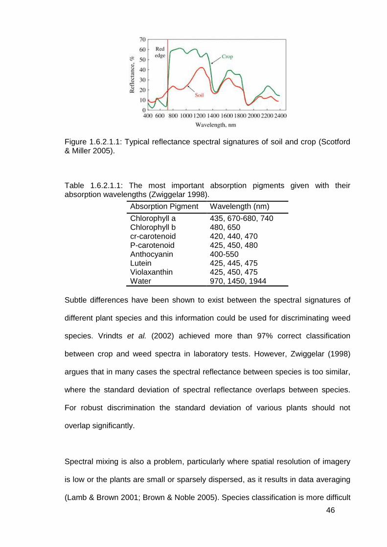
reflectance, transmission and absorption of light at different wavelengths (Figure

1.6.2.1.1) (Borregard et al. 2000). The spectral absorption and reflectance from

plants is a feature of the absorption pigments that plants contain and the physical

structure of the surface and the cells in the leaves (Zwiggelar 1998). The most

important pigments for absorption are given with their absorption wavelengths in

Table 1.6.2.1.1. The high reflectance in the near-infrared (NIR) region of the

spectrum is caused by scattering from the air/water/cell wall interfaces within

leaves (Zwiggelar 1998). Increasing leaf area increases reflectance in the NIR

region of the spectrum as the area of scattering surfaces increases (Asner 1998).

46

Figure 1.6.2.1.1: Typical reflectance spectral signatures of soil and crop (Scotford & Miller 2005).

Table 1.6.2.1.1: The most important absorption pigments given with their absorption wavelengths (Zwiggelar 1998).

Absorption Pigment Wavelength (nm)

Chlorophyll a 435, 670-680, 740 Chlorophyll b 480, 650 cr-carotenoid 420, 440, 470 P-carotenoid 425, 450, 480 Anthocyanin 400-550 Lutein 425, 445, 475 Violaxanthin 425, 450, 475 Water 970, 1450, 1944

Subtle differences have been shown to exist between the spectral signatures of

different plant species and this information could be used for discriminating weed

species. Vrindts et al. (2002) achieved more than 97% correct classification

between crop and weed spectra in laboratory tests. However, Zwiggelar (1998)

argues that in many cases the spectral reflectance between species is too similar,

where the standard deviation of spectral reflectance overlaps between species.

For robust discrimination the standard deviation of various plants should not

overlap significantly.

Spectral mixing is also a problem, particularly where spatial resolution of imagery

is low or the plants are small or sparsely dispersed, as it results in data averaging

(Lamb & Brown 2001; Brown & Noble 2005). Species classification is more difficult

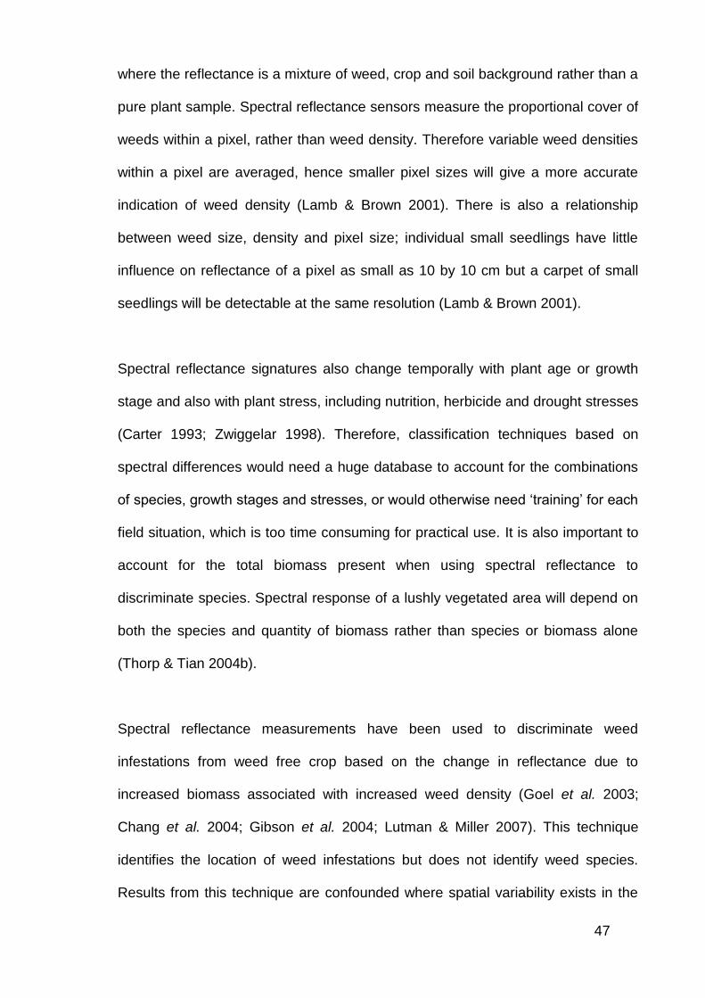
47

where the reflectance is a mixture of weed, crop and soil background rather than a

pure plant sample. Spectral reflectance sensors measure the proportional cover of

weeds within a pixel, rather than weed density. Therefore variable weed densities

within a pixel are averaged, hence smaller pixel sizes will give a more accurate

indication of weed density (Lamb & Brown 2001). There is also a relationship

between weed size, density and pixel size; individual small seedlings have little

influence on reflectance of a pixel as small as 10 by 10 cm but a carpet of small

seedlings will be detectable at the same resolution (Lamb & Brown 2001).

Spectral reflectance signatures also change temporally with plant age or growth

stage and also with plant stress, including nutrition, herbicide and drought stresses

(Carter 1993; Zwiggelar 1998). Therefore, classification techniques based on

spectral differences would need a huge database to account for the combinations

of species, growth stages and stresses, or would otherwise need ‘training’ for each

field situation, which is too time consuming for practical use. It is also important to

account for the total biomass present when using spectral reflectance to

discriminate species. Spectral response of a lushly vegetated area will depend on

both the species and quantity of biomass rather than species or biomass alone

(Thorp & Tian 2004b).

Spectral reflectance measurements have been used to discriminate weed

infestations from weed free crop based on the change in reflectance due to

increased biomass associated with increased weed density (Goel et al. 2003;

Chang et al. 2004; Gibson et al. 2004; Lutman & Miller 2007). This technique

identifies the location of weed infestations but does not identify weed species.

Results from this technique are confounded where spatial variability exists in the

48

background crop growth in addition to the weed density. Lamb et al. (1999)

performed comparisons between density data for Avena spp. and the normalised

difference vegetation index (NDVI) or the soil-adjusted vegetation index (SAVI) at

resolutions of 0.5, 1.0, 1.5 and 2.0 m in a triticale crop where the triticale and

Avena spp. were at the 2-5 leaf stage. The highest correlations were achieved at

0.5 m resolution (up to 71%) and the lowest at 2 m. At the 0.5 m resolution they

found that the NDVI images could not reliably discriminate weed populations of

less than 28 plants m-2 from weed free areas and the SAVI could not reliably

discriminate weed populations of less than 17 plants m-2. This is a significant

improvement in discrimination given that in each case, the SAVI only provided an

increase in R2 of 1-2% over the NDVI.

The success of this approach and the weed densities that can be detected will be

affected by differences in growth rates of weed and crop, time of emergence,

differences in vigour and timing of inflorescence and senescence (Lamb & Brown

2001). López-Granados et al. (2006) suggest that high resolution satellite imagery

acquired 2-3 weeks prior to crop senescence could be used to detect grass weeds

in wheat, as the grass weeds mature later and remain green after the crop has

started to lose its green colour. This map could be used to direct herbicide

application in the following season.

Many studies judge the success or failure of weed mapping attempts on the ability

to reliably identify weed species. It is not necessary to achieve identification of

weeds to a species level for SSWM, rather all weeds controlled by the same

treatment can be placed in the same class and this may improve classification

accuracy (Lamb & Brown 2001; Vrindts et al. 2002). Also, most studies ignore the

49

valuable information that can be gained from farm operators. Farm operators

generally know from prior farm operations such as seeding and harvest what weed

species can be expected, and where they are likely to be concentrated, and this

information can be used to aid in image classification and in the creation of

prescription maps (Lamb & Brown 2001).

Currently, herbicide recommendations tend to be based on weed species, weed

size, growth stage and density. Therefore, to create a prescription map from

sensor data requires relationships between sensor data and these plant

characteristics. Largely the detail of these relationships is lacking; sensor data has

been shown to adequately identify weed infestation locations but the sensor data

may not fully describe the significance of the weed infestation and the amount of

herbicide required for adequate control (Lamb & Brown 2001; Thorp & Tian

2004a).

Classification errors of weed species or class can fall into two categories; omission

and commission. Omission occurs when a plant belonging to a certain class is

classified as something else, commission occurs when a plant from another class

is classified as the class of interest (Lamb & Brown 2001).

1.6.2.2 Remote and proximal sensing

Remote sensing platforms for weed research have included balloons, remote

control craft, airplanes and satellites (Thorp & Tian 2004b). Data is acquired from

remote sensing systems and processed prior to spraying, the decision on what

herbicide to apply is already made and the computing load on the sprayer control

50

system is reduced (Brown & Noble 2005). Proximal sensors provide the

opportunity for real time decision making, requiring much greater computational

capacity of the control system, and there is no prior information on how much

herbicide will be required. There is greater control over data acquisition from

proximal sensors and the turnaround time for data delivery is in the order of

seconds to hours rather than days to weeks required for remote sensing, they tend

to be higher resolution and data acquisition opportunities are not affected by

overcast conditions and platform availability (Scotford & Miller 2005).

The first real time patch sprayer was developed by Haggar et al. (1983) and used

measurements of reflectance in the red and NIR regions of the spectrum to

activate a spray nozzle when green vegetation was sensed. However, according

to Felton et al. (2002) the device could not perform under variable light and

background conditions. The Weedseeker is a commercially available system for

site specific management of weeds. The Weedseeker uses an active light source

in the red and NIR regions, therefore readings are independent of variations in

illumination and a spray nozzle is activated when green vegetation is sensed.

However, this system is only for use in fallow situations or between rows in wide

row cropping systems, where green weeds can be sensed against a soil or crop

residue background. There are no commercially available systems for

discriminating weeds from crop plants using remote sensing.

Remote sensing data is limited to wavelengths above the ultraviolet and blue

range due to atmospheric scattering (Brown & Noble 2005) and cannot provide

information on the water absorption bands of the vegetation, as the water in the

51

atmosphere absorbs the light at these wavelengths before it reaches the

underlying vegetation (Henry et al. 2004).

1.6.3 Machine vision

Machine vision systems often use charge coupled device (CCD) cameras

mounted between 1-2 m above the target field of view, providing down to one mm

pixel resolution in the imagery. This imagery provides highly detailed information at

a fine scale; as such it has large requirements for computing power (Keränen et al.

2003; Thorp & Tian 2004b). The appropriate image resolution for plant

identification from shape parameters is likely to vary according to local field

conditions, in particular weed size. The pixel size should be adjusted to be smaller

than the plants during image collection (Yang et al. 2003). These cameras provide

multispectral information in the red, green and blue (RGB) colour space for

discriminating green vegetation from soil and residue backgrounds. The addition of

NIR to the RGB information would be ideal, allowing calculation of indices such as

NDVI. Such cameras are available; however their cost is much greater than a

typical machine vision camera (Brown & Noble 2005).

The main steps in machine vision image processing and analysis include (1)

image acquisition; (2) identification of vegetation pixels and image segmentation;

(3) feature extraction; (4) classification; and (5) estimation of weed number based

on size, shape, texture and colour features of the identified plant segments

(Andreason et al. 1997; Gebhardt et al. 2006).

52

The simplest use of machine vision for weed mapping exploits the consistent

distance that exists between crop rows in most cultivated crops. Hague et al.

(2006) describe a method where the red, green and blue channels of a

conventional CCD camera are used to discriminate plants from their soil

background. A priori knowledge of the distance between crop rows and the

consistent nature of crop rows is then used to identify crop rows within the image

and exclude them from the analysis. Plants identified as growing in the inter-row

were classified as weeds based on the assumption that a weed is a plant growing

out of place. This approach also assumes that weed density in the inter-row is

representative of weed density in the row (Yang et al. 2003; Hague et al. 2006).

This may not always be the case in Australian cropping systems, where pre-

emergent herbicides such as trifluralin are concentrated in the inter-row by the

movement of treated soil by tillage during crop planting, resulting in lower weed

densities of certain weed species between the rows. However, it should still

provide information on where weed densities are changing in the row. The

automated approach used by Hague et al. (2006) had a strong correlation

(R2=0.91) with the manual assessment of weed density. This approach does not

provide information on weed species, but could be used in conjunction with prior

farmer knowledge to create useful prescription maps. Hague et al. (2006)

performed their study in a cereal crop on 25 cm spacing. This is considered widely

spaced for UK cropping systems (Lutman & Miller 2007), but would be considered

the norm in Australian cropping systems. Gerhards and Oebel (2006) found that

beyond Zadoks growth stage 25 overlapping of cereals in the inter row made

species identification from shape parameters impossible; however it is not

specified what the row spacing was in this instance.

53

More complex image recognition systems take this process further. Plants that are

identified in the inter-row have features of shape, texture and colour extracted from

the image to help classify plants into weed species. Close proximity of weeds to

crop rows can make weed identification difficult and lead to misclassification

(Grundy et al. 2005). Several studies have achieved high classification accuracies

in wider row crops such as lettuce (Blasco et al. 2002), tomato (Lee et al. 1999)

and corn (Yang et al. 2002). The identification of crop rows reduces the number of

objects on which shape analysis need to be performed, therefore reducing the

image classification time (Pérez et al. 2000; Yang et al. 2003).

Weed species identification from shape based features are hampered by occluded

or overlapping leaves, wind, variations in plant leaf size and shape as a function of

growth stage, and the variable three dimensional orientation of leaves in relation to

the machine vision sensor (Moshou et al. 2002; Thorp & Tian 2004b; Brown &

Noble 2005). In addition to this, varying illumination conditions in the field can

make image capture more difficult (Moshou et al. 2002). Pérez et al. (2000) found

that image processing was more difficult on sunny days due to highlights and

shadows in the images. To overcome this they introduced a light diffuser to reduce

the effects of natural illumination.

Many shape based features have been extracted from imagery and many

transformations performed in studies for the purpose of species identification.

Shape based parameters including complexity, elongatedness, central moment

and principle axis moment have been used (Thorp & Tian 2004b). Boundary

transformations include Fourier analysis, curve fitting and a technique using the

radial distance from the geometric centre of the leaf (Brown & Noble 2005). Other

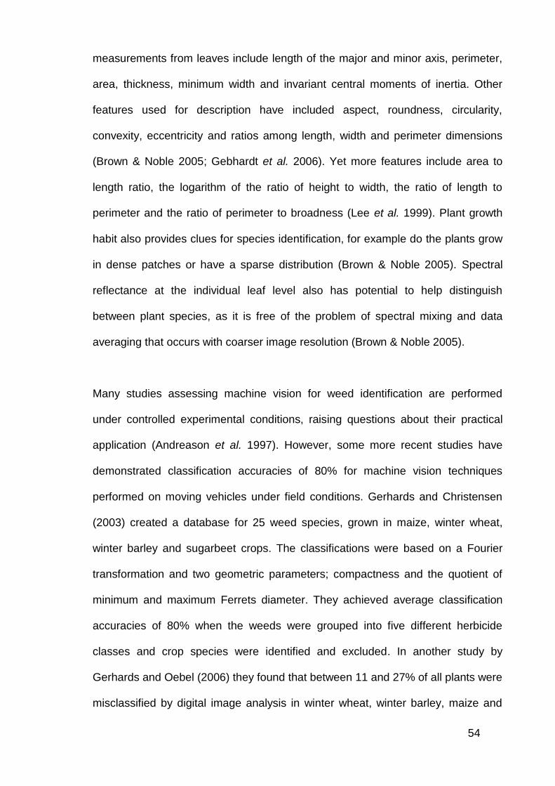
54

measurements from leaves include length of the major and minor axis, perimeter,

area, thickness, minimum width and invariant central moments of inertia. Other

features used for description have included aspect, roundness, circularity,

convexity, eccentricity and ratios among length, width and perimeter dimensions

(Brown & Noble 2005; Gebhardt et al. 2006). Yet more features include area to

length ratio, the logarithm of the ratio of height to width, the ratio of length to

perimeter and the ratio of perimeter to broadness (Lee et al. 1999). Plant growth

habit also provides clues for species identification, for example do the plants grow

in dense patches or have a sparse distribution (Brown & Noble 2005). Spectral

reflectance at the individual leaf level also has potential to help distinguish

between plant species, as it is free of the problem of spectral mixing and data

averaging that occurs with coarser image resolution (Brown & Noble 2005).

Many studies assessing machine vision for weed identification are performed

under controlled experimental conditions, raising questions about their practical

application (Andreason et al. 1997). However, some more recent studies have

demonstrated classification accuracies of 80% for machine vision techniques

performed on moving vehicles under field conditions. Gerhards and Christensen

(2003) created a database for 25 weed species, grown in maize, winter wheat,

winter barley and sugarbeet crops. The classifications were based on a Fourier

transformation and two geometric parameters; compactness and the quotient of

minimum and maximum Ferrets diameter. They achieved average classification

accuracies of 80% when the weeds were grouped into five different herbicide

classes and crop species were identified and excluded. In another study by

Gerhards and Oebel (2006) they found that between 11 and 27% of all plants were

misclassified by digital image analysis in winter wheat, winter barley, maize and

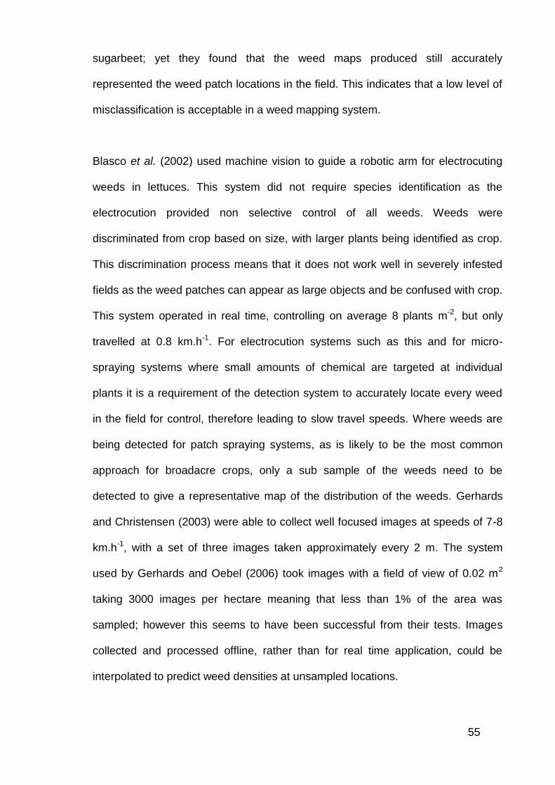
55

sugarbeet; yet they found that the weed maps produced still accurately

represented the weed patch locations in the field. This indicates that a low level of

misclassification is acceptable in a weed mapping system.

Blasco et al. (2002) used machine vision to guide a robotic arm for electrocuting

weeds in lettuces. This system did not require species identification as the

electrocution provided non selective control of all weeds. Weeds were

discriminated from crop based on size, with larger plants being identified as crop.

This discrimination process means that it does not work well in severely infested

fields as the weed patches can appear as large objects and be confused with crop.

This system operated in real time, controlling on average 8 plants m-2, but only

travelled at 0.8 km.h-1. For electrocution systems such as this and for micro-

spraying systems where small amounts of chemical are targeted at individual

plants it is a requirement of the detection system to accurately locate every weed

in the field for control, therefore leading to slow travel speeds. Where weeds are

being detected for patch spraying systems, as is likely to be the most common

approach for broadacre crops, only a sub sample of the weeds need to be

detected to give a representative map of the distribution of the weeds. Gerhards

and Christensen (2003) were able to collect well focused images at speeds of 7-8

km.h-1, with a set of three images taken approximately every 2 m. The system

used by Gerhards and Oebel (2006) took images with a field of view of 0.02 m2

taking 3000 images per hectare meaning that less than 1% of the area was

sampled; however this seems to have been successful from their tests. Images

collected and processed offline, rather than for real time application, could be

interpolated to predict weed densities at unsampled locations.

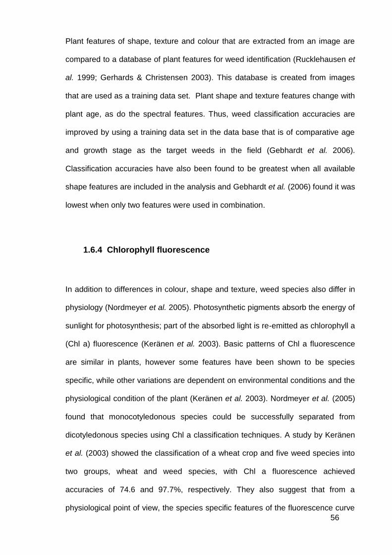
56

Plant features of shape, texture and colour that are extracted from an image are

compared to a database of plant features for weed identification (Rucklehausen et

al. 1999; Gerhards & Christensen 2003). This database is created from images

that are used as a training data set. Plant shape and texture features change with

plant age, as do the spectral features. Thus, weed classification accuracies are

improved by using a training data set in the data base that is of comparative age

and growth stage as the target weeds in the field (Gebhardt et al. 2006).

Classification accuracies have also been found to be greatest when all available

shape features are included in the analysis and Gebhardt et al. (2006) found it was

lowest when only two features were used in combination.

1.6.4 Chlorophyll fluorescence

In addition to differences in colour, shape and texture, weed species also differ in

physiology (Nordmeyer et al. 2005). Photosynthetic pigments absorb the energy of

sunlight for photosynthesis; part of the absorbed light is re-emitted as chlorophyll a

(Chl a) fluorescence (Keränen et al. 2003). Basic patterns of Chl a fluorescence

are similar in plants, however some features have been shown to be species

specific, while other variations are dependent on environmental conditions and the

physiological condition of the plant (Keränen et al. 2003). Nordmeyer et al. (2005)

found that monocotyledonous species could be successfully separated from

dicotyledonous species using Chl a classification techniques. A study by Keränen

et al. (2003) showed the classification of a wheat crop and five weed species into

two groups, wheat and weed species, with Chl a fluorescence achieved

accuracies of 74.6 and 97.7%, respectively. They also suggest that from a

physiological point of view, the species specific features of the fluorescence curve

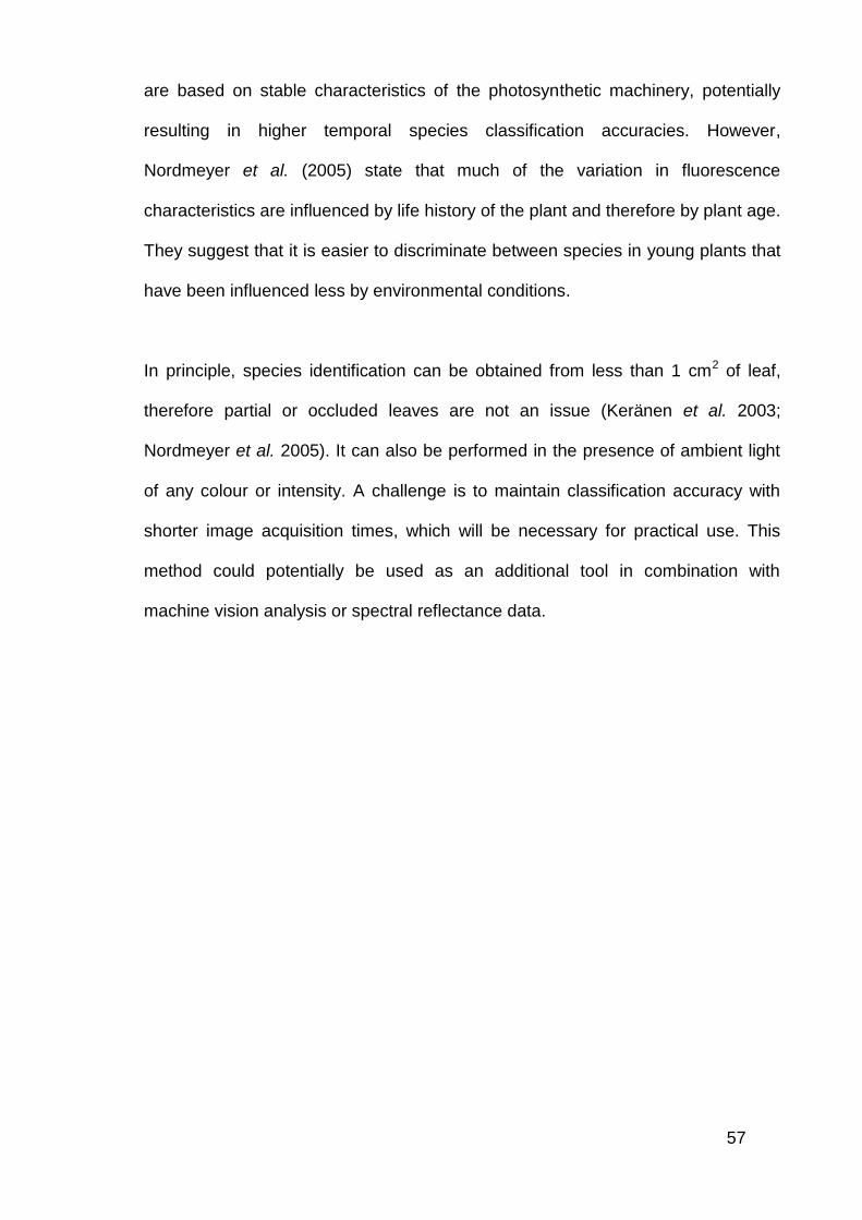
57

are based on stable characteristics of the photosynthetic machinery, potentially

resulting in higher temporal species classification accuracies. However,

Nordmeyer et al. (2005) state that much of the variation in fluorescence

characteristics are influenced by life history of the plant and therefore by plant age.

They suggest that it is easier to discriminate between species in young plants that

have been influenced less by environmental conditions.

In principle, species identification can be obtained from less than 1 cm2 of leaf,

therefore partial or occluded leaves are not an issue (Keränen et al. 2003;

Nordmeyer et al. 2005). It can also be performed in the presence of ambient light

of any colour or intensity. A challenge is to maintain classification accuracy with

shorter image acquisition times, which will be necessary for practical use. This

method could potentially be used as an additional tool in combination with

machine vision analysis or spectral reflectance data.

58

1.7 Resolution, Interpolation and Map Production

‘Offline’ treatment of weed patches requires the production of a weed map that can

be used to control where the patch sprayer applies herbicide with location

information provided from a GPS. The aim is to produce a map that best

represents the actual weed distribution and densities. Map quality is assessed on

this basis, rather than just creating a visually attractive map. Many maps are

constructed from sample data collected at widely spaced intervals and spatial

interpolation is used to predict weed densities at unobserved locations as well as

re-estimating densities at observed locations (Dille et al. 2002). This contrasts with

satellite and aerial imagery where pixels are contiguous. For weed maps created

from data collected at widely spaced intervals the quality of the map will depend

on the distance between observations, the size of the observation support area

(i.e. quadrat size or field of view) and the method of spatial interpolation.

Kriging has been the most popular method of spatial interpolation for weeds data

(Rew & Cousens 2001). However, geostatistical interpolation methods were

developed for earth sciences where data generally follow a smooth continuum,

whereas weed data tend to be characterised by large proportions of data recording

zero with smaller proportions recording high values and often in sharp peaks (Rew

& Cousens 2001). Several studies have showed that kriging is a poor estimator of

weed density, where the procedure tends to smooth the data too much, levelling

the peaks of weed density and interpolating weeds into locations where they are

not present (Zanin et al. 1998; Rew et al. 2001). Dille et al. (2002) compared the

performance of four interpolation methods including inverse-distance weighting,

59

ordinary point kriging, minimum surface curvature and multiquadratic basis

function. They found that all of these interpolation methods underestimated high

density portions of fields and overestimated low density areas and were

particularly poor in fields with low infestation levels. Gerhards et al. (1997) used

linear triangulation for interpolation of weeds data and found it to be more accurate

than ordinary kriging. However, adequate sampling is of more importance than the

spatial interpolation method used (Lutman & Miller 2007).

A study by Cousens et al. (2002) analysed a data set of 225,000 quadrat counts of

capeweed completely covering a 0.9 ha area. They found that quadrat size had

much less effect on map detail than quadrat spacing, although some spatial

variation at the sub meter level was lost because larger quadrats increasingly

average out information and reflect more general trends. Quadrat size in this study

is analogous to pixel size of satellite and aerial imagery and the field of view of

proximal sensors. Quadrat spacing was found to be very important in describing

fine scale variation, which may include localised regions well above any economic

threshold for herbicide applications. For example, dense patches of weeds may be

missed completely if their diameters are smaller than the distance between

quadrat spacings. Quadrat spacing in this study is analogous to the spacing

between proximal sensors. In addition to the potential for missing small patches,

coarser sampling strategies exacerbate errors associated with spatial

interpolation; with greater areas recorded as weedy than would be present

(Lutman & Perry 1999; Rew & Cousens 2001).

The economic benefits associated with SSWM are related to the proportion of the

field that is weed infested, the number of weed patches and the spatial resolution

60

of sampling and spraying technologies (Rew et al. 1997, Wallinga et al. 1998;

Lutman & Perry 1999; Barroso et al. 2004). Wallinga et al. (1998) estimated the

herbicide use for a patch sprayer that operated at spatial resolutions of 0.5, 1, 2

and 4 metre resolution. The idealised patch sprayer could detect all weeds of

Galium aparine and the treatment threshold was the presence of G. aparine at any

density at that scale of resolution. At a resolution of 4 m 85% of the field would be

sprayed, at 2 m resolution 62% would be sprayed, at 1 m resolution 41% would be

sprayed while at 0.5 m only 26% of the field would be sprayed. Taking this further,

the greatest saving is achieved when only the weed leaves are treated. However,

the benefits in herbicide reduction in operating at this scale need to be balanced

with the costs of mapping weeds at this scale and the engineering cost of

achieving the desired spray application (Lutman & Miller 2007). A study in Spain

on Avena ludoviciana found that profitability of SSWM increased as the proportion

of the field infested decreased and that when 64% or more of the field was

infested SSWM was never profitable (Barroso et al. 2004). They found that errors

in mapping increased with coarser mapping resolution and when patch number

increased. At the same time, errors in spraying increased when mapping and

spraying resolution decreased and when patch number increased. The cost of

herbicide waste, that is applying herbicide where there are no weeds, increased

with increases in infested area and patch number and declined with higher

mapping and spraying resolution. The model assumed costs for various levels of

technology for mapping and spraying: € 9.0 ha-1 for 12 m resolution, € 13.5 ha-1 for

6 m resolution and € 27.0 ha-1 for 3 m resolution, although they do recognise that it

is difficult to assign values to technology that is still under development. Based on

these costs it became profitable to employ SSWM when 30% of the field was

infested, but only with mapping and spraying resolutions of 6 or 12 m. The highest

61

net returns were obtained when 14% of the field was infested with a single patch

and a 12 m mapping and spraying resolution.

The field of view, spacing and position of sensors becomes even more important

when weed patches have distributions that exhibit anisotropy. Isotropy occurs

when weed patches display radial symmetry in weed density and reflects natural

dispersal (Humston et al. 2005). Anisotropy occurs when weed patches display

directionality in shape and indicates the presence of two distinct spatial

distributions or an additional source of variability in one direction (Blanco-Moreno

et al. 2006). Many fields are managed primarily in one direction (Rew & Cousens

2001) and with the increased adoption of GPS guidance, Autosteer and controlled

traffic farming this is likely to have increased. This leads to dispersal of seeds by

cultivation and harvesters in the direction of travel and results in elongated

patches. Dispersal of weed seeds by cultivation is only over short distances and

Rew and Cussans (1997) found that 84% of seeds are moved less than 1m from

their source with tine machines, it is expected that seed movement would be even

less with knife point and disc seeding systems. Movement of weed seeds by

harvesters has been found to be far more important in the development of

anisotropy, particularly where the weed species retains the majority of its seed on

the plant at the time of crop harvest; such is the case with annual ryegrass.

Blanco-Moreno et al. (2004) found that dispersal of annual ryegrass by harvesters

can exceed 18 m although the modal dispersal was close to the origin. They also

found that lateral movement and the concentration of seed in the chaff row is more

relevant than longitudinal dispersal in the development of patterns of seedlings.

62

This potentially has three important implications for site specific management:

1. The resolution of mapping and the placement of sensors. To ensure the

highest density patches are mapped sensors would need to be mounted

above harvester chaff rows to map the weeds growing in these rows.

2. The resolution capacity of spray application equipment.

3. The need for remapping or the addition of buffers around patches to

account for seed dispersal. Weed seed dispersal aided by harvesters is 16

fold greater than unaided dispersal for Bromus sp (Woolcock & Cousens

2000). Rapidly spreading weeds with unpredictable patches will need to be

remapped more readily than sedentary weed patches. Rew et al. (1997)

recommend adding a 4 metre buffer around patches to account for seed

movement, navigation errors and sprayer response times. The addition of

this buffer increased the area to be sprayed by an average of 10.6%, but

fields with few larger patches were less affected by the addition of buffers

than fields with numerous small patches. The data for annual ryegrass

seed movement by harvesters may suggest that much larger buffers would

need to be used when using maps in subsequent years to account for seed

dispersal, which will reduce the savings in herbicide achieved by SSWM.

The use of chaff carts for catching weed seeds that pass through harvesting

machinery may reduce the anisotropic effects caused by seed dispersal through

harvesters.

63

1.8 Research Aims

The aims of this study were to

1. Assess techniques for mapping annual ryegrass density using spectral

reflectance sensors,

2. Assess the spatial stability of annual ryegrass density over several

seasons,

3. Determine the relationship between annual ryegrass density and herbicide

efficacy, and

4. Assess the herbicide options for differential control of high and low density

annual ryegrass populations and determine the strategies for best

economic outcome.

64

2 Mapping Lolium rigidum Patches Using Spectral

Reflectance Sensors

2.1 Introduction

Spectral reflectance measurements have been used to discriminate weed

infestations from weed free crop based on the change in reflectance due to

increased biomass associated with increased weed density (Goel et al. 2003;

Chang et al. 2004; Gibson et al. 2004; Lutman & Miller 2007). This technique

coupled with GPS positioning identifies the location of weed infestations, but does

not identify weed species or absolute density. Results from this technique are

confounded where spatial variability exists in both the background crop growth and

the weed density. Lamb et al. (1999) performed comparisons between density

data for Avena spp. and the normalised difference vegetation index (NDVI) or the

soil-adjusted vegetation index (SAVI) at resolutions of 0.5, 1.0, 1.5 and 2.0 m in a

triticale crop when the triticale and Avena spp. were at the 2-5 leaf stage. The

highest correlations were achieved at 0.5 m resolution (up to 71%) and the lowest

at 2 m. At the 0.5 m resolution they found that the NDVI images could not reliably

discriminate weed populations of less than 28 plants m-2 from weed free areas and

the SAVI could not reliably discriminate weed populations of less than 17 plants m-

2. This is a significant improvement in discrimination given that in each case, the

SAVI only provided an increase in R2 of 1-2% over the NDVI.

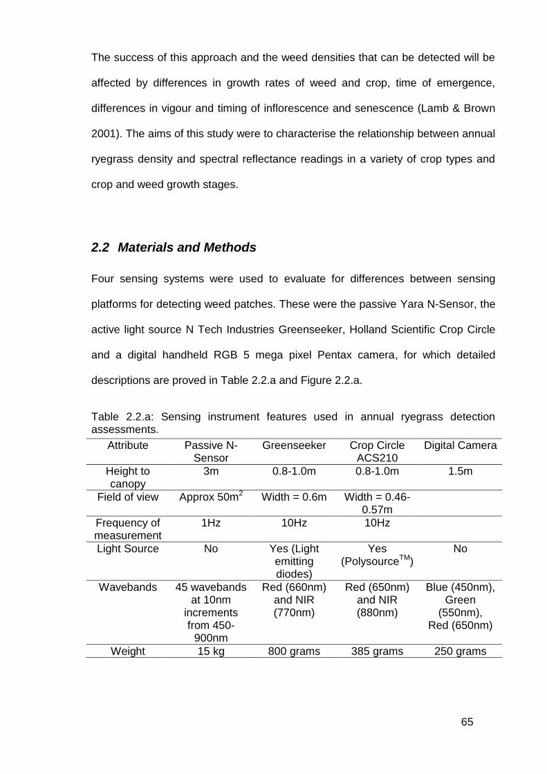
65

The success of this approach and the weed densities that can be detected will be

affected by differences in growth rates of weed and crop, time of emergence,

differences in vigour and timing of inflorescence and senescence (Lamb & Brown

2001). The aims of this study were to characterise the relationship between annual

ryegrass density and spectral reflectance readings in a variety of crop types and

crop and weed growth stages.

2.2 Materials and Methods

Four sensing systems were used to evaluate for differences between sensing

platforms for detecting weed patches. These were the passive Yara N-Sensor, the

active light source N Tech Industries Greenseeker, Holland Scientific Crop Circle

and a digital handheld RGB 5 mega pixel Pentax camera, for which detailed

descriptions are proved in Table 2.2.a and Figure 2.2.a.

Table 2.2.a: Sensing instrument features used in annual ryegrass detection assessments.

Attribute Passive N-Sensor

Greenseeker Crop Circle ACS210

Digital Camera

Height to canopy

3m 0.8-1.0m 0.8-1.0m 1.5m

Field of view Approx 50m2 Width = 0.6m Width = 0.46-0.57m

Frequency of measurement

1Hz

10Hz 10Hz

Light Source No Yes (Light emitting diodes)

Yes (PolysourceTM)

No

Wavebands 45 wavebands at 10nm

increments from 450-

900nm

Red (660nm) and NIR (770nm)

Red (650nm) and NIR (880nm)

Blue (450nm), Green

(550nm), Red (650nm)

Weight 15 kg 800 grams 385 grams 250 grams

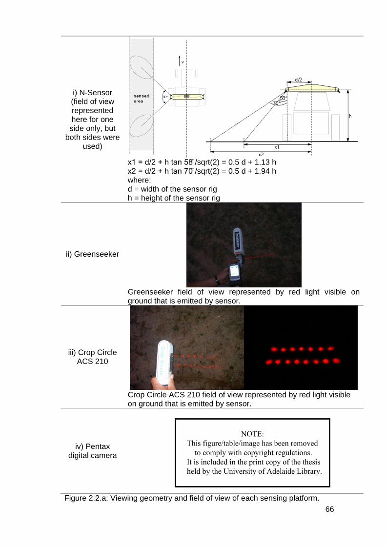
66

i) N-Sensor (field of view represented here for one side only, but

both sides were used)

x1 d 2 h tan /sqrt(2) = 0.5 d + 1.13 h x2 d 2 h tan 70 /sqrt(2) = 0.5 d + 1.94 h where: d = width of the sensor rig h = height of the sensor rig

ii) Greenseeker

Greenseeker field of view represented by red light visible on ground that is emitted by sensor.

iii) Crop Circle ACS 210

Crop Circle ACS 210 field of view represented by red light visible on ground that is emitted by sensor.

iv) Pentax digital camera

Figure 2.2.a: Viewing geometry and field of view of each sensing platform.

A NOTE:

This figure/table/image has been removed to comply with copyright regulations. It is included in the print copy of the thesis held by the University of Adelaide Library.

67

2.2.1 Stationary sensor measurement

Continuous monitoring sites were established in two farmers’ fields in 2008.

Ronnies Paddock (-33.8867, 137.8975) is located near the town of Bute (South

Australia) and was sown with cv. Nugget lentils on 12/05/08. Measurements were

obtained at five growth stages (Table 2.2.1.a). The fifth timing date was after an

application of clethodim (80 g ha-1) and quizalofop (10 g ha-1) on 15/07/08 for

annual ryegrass control. Diflufenican (75 g ha-1) was also applied for broadleaf

weed control on 20/06/08. Annual ryegrass densities across the site ranged from

0-1600 plants m-2. Stones South Paddock (-34.2238, 138.7108) is located near the

town of Tarlee (South Australia) and was sown with cv. Kaspa peas on 1/6/2008.

Measurements were obtained at four growth stages (Table 2.2.1.b). Annual

ryegrass densities across the site ranged from 0-2000 plants m-2. Stationary N-

Sensor measurements were collected at 20 and 21 monitoring locations in

Ronnies and Stones South, respectively. These sites were GPS referenced and

pegged, so that on each measurement date the measurements were made at the

same location, by parking the mounting vehicle in the same spot relative to the

peg. The GPS was a KEE technologies Triple X receiver with sub metre accuracy.

In the centre of each quadrant of the N-Sensors field of view (Figure 2.2.a.i)

measurements were also taken with the Greenseeker, and Crop Circle, and digital

images were collected with the RGB digital camera, equating to 80 and 84 data

points in Ronnies and Stones south, respectively. These sites form the monitoring

sites for density measurement. At the 80 monitoring sites in Ronnies, annual

ryegrass and lentil density were measured on 04/06/08. Medicago scutellata (snail

medic) density was also found to vary in Ronnies paddock. To account for this

Medic density was recorded on 01/07/08. Avena fatua (wild oat) density was

observed to vary at Stones South. At the 84 monitoring sites in Stones South

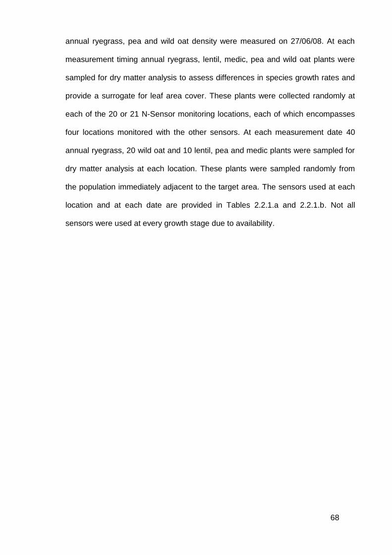
68

annual ryegrass, pea and wild oat density were measured on 27/06/08. At each

measurement timing annual ryegrass, lentil, medic, pea and wild oat plants were

sampled for dry matter analysis to assess differences in species growth rates and

provide a surrogate for leaf area cover. These plants were collected randomly at

each of the 20 or 21 N-Sensor monitoring locations, each of which encompasses

four locations monitored with the other sensors. At each measurement date 40

annual ryegrass, 20 wild oat and 10 lentil, pea and medic plants were sampled for

dry matter analysis at each location. These plants were sampled randomly from

the population immediately adjacent to the target area. The sensors used at each

location and at each date are provided in Tables 2.2.1.a and 2.2.1.b. Not all

sensors were used at every growth stage due to availability.

69

Table 2.2.1.a: Site and sensing details for five sensing dates in lentils in Ronnies paddock near Bute in 2008.

Date

Cloud cover (%)

Growth Stage Dry Matter Sensors Used

Lentil Annual

ryegrass Lentils

Annual ryegrass

Medic GS N-

Sensor Camera

04/06/08

70 4 node 11 - 12 Y Y N Y Y Y

15/06/08

0 7 node 11 – 22 Y Y N Y Y Y

01/07/08

70 9 – 10 node

12 – 23 Y Y Y Y Y Y

12/07/08

80 10 - 12 node

13 - 25 Y Y Y Y Y Y

21/08/08

Pre flower

Y N Y Y Y Y

Table 2.2.1.b: Site and sensing details for four sensing dates in field peas in Stones South paddock near Tarlee in 2008.

Date

Cloud cover (%)

Growth Stage Dry Matter Sensors Used

Pea Annual

ryegrass Pea

Annual ryegrass

Wild oat

GS CC N-

Sensor Camera

27/06/08

25 2 - 3 node

11 - 12 Y Y Y Y N Y Y

11/07/08

30 5 node 11 – 22 Y Y Y Y Y Y Y

29/07/08

90 6 – 7 node

11 – 23 Y Y Y Y Y Y Y

26/08/08

0 11 – 12 node

11 - 25 Y Y Y N Y Y Y

70

The N-Sensor measurements taken were stationary. Greenseeker and Crop Circle

measurements were taken with the sensor in motion, scanning a 1m pass over the

monitoring location. The N-Sensor provides reflectance data for 45 wavebands

from 450 to 900nm, while the Greenseeker and Crop Circle provides NDVI based

on the red and NIR reflectance measurements. Two digital camera images were

collected at each site from 1.5 m directly above the point and from 3 m in front of

the point and from a height of 1.5 m (27˚ above the horizontal) (Table 2.2.1.d).

Pixels in the images were classified as plant or not plant using an Excessive

Green – Excessive Red (ExG – ExR) algorithm,

ExG – ExR = (2*G – R – B) – (1.4*R – G)

where R, G and B are the red, green and blue pixel values from the image (Meyer

& Camargo Neto, 2008). A binary image was produced from which total green

plant cover could be calculated.

Linear and non-linear regression was performed to determine the goodness of the

fit between annual ryegrass density and sensor response and reported as the

coefficient of determination (R2). Non linear regression was of the form where the

natural log of annual ryegrass density (x axis) was regressed with the linear

sensor response (y axis), i.e. y = a*ln(x) + b. The slope of the response curve is

also important. The slope indicates the sensor responsiveness to change in

annual ryegrass density, where a steeper slope indicates the sensor is more

responsive to increasing annual ryegrass density. Therefore, for regressions that

produce a similar R2 the curve with the steeper slope will be more useful for

discriminating ryegrass density based on sensor response. Slope comparisons

were analysed using Extra sum of squares F-test in Prism 6.03.

71

2.2.1.1 Optimised vegetative indices for annual ryegrass detection

Principal components analysis (PCA) was carried out between the reflectance

data for each wavelength measured with the N-Sensor and the ryegrass density in

Ronnies and Stones South paddock using the software Sirius version 7.1. PCA

was repeated for each date that sensor measurements were collected.

Wavelengths with the strongest correlation coefficient (r) with ryegrass density

were used in NDVI and simple ratio (SR) type equations:

NDVI = (Rx nm – Ry nm) / (Rx nm + Ry nm), and

SR = Rx nm / Ry nm

Where Rx nm and Ry nm is the reflectance measured at x and y nm respectively.

These indices were regressed with ryegrass density to determine which index

provided the best coefficient of determination (R2). These were also compared with

the biomass index output directly from the N-Sensor

BI = 10*(R740nm/R720nm – 1)

Where R740nm is the reflectance measured at 740nm and R720nm is the reflectance

measured at 720nm. NDVI calculations that include NIR and either red, green,

blue or some other visible wavelength will be described by the colour, i.e. an NDVI

calculated from NIR (780 nm) and red (670 nm) will be described as NDVI (red).

Non-linear regression was performed to determine the goodness of the fit between

annual ryegrass density and sensor response and reported as the coefficient of

determination (R2). Non linear regression was of the form where the natural log of

annual ryegrass density (x axis) was regressed with the linear sensor response (y

axis). Slope comparisons were analysed using Extra sum of squares F-test in

Prism 6.03. All indices were forced onto a similar scale for comparison of slope,

72

that is in the range 0-1, comparable with the range of NDVI. Simple ratio (SR) and

biomass index (BI) indices were divided by 10 to make this comparison.

2.2.1.2 Optimised camera position for annual ryegrass detection

Two digital camera images were collected at each site from 1.5 m directly above

the point and from 3 m in front of the point and from a height of 1.5 m (27˚ above

the horizontal). The ExG – ExR algorithm was used to determine the percentage

of green pixels in each image. Linear and log functions were fitted between the

algorithm output and annual ryegrass density to determine which camera position

was best able to differentiate annual ryegrass density.

Non-linear regression was performed to determine the goodness of the fit between

annual ryegrass density and percent area identified as plant and reported as the

coefficient of determination (R2). Non linear regression was of the form where the

natural log of annual ryegrass density (x axis) was regressed with the linear

camera response (y axis). Slope comparisons were analysed using Extra sum of

squares F-test in Prism 6.03.

2.2.1.3 Spatial scale of measurements.

N-Sensor measurements were collected at 20 and 21 GPS referenced locations in

Ronnies and Stones South respectively. Measurements were collected with the

Greenseeker and digital camera in the 4 quadrants of the N-Sensor field of view,

totalling 80 and 84 measurement points with these two sensors in Ronnies and

Stones South respectively. Annual ryegrass was counted at each of these points.

73

Natural log curves were fitted to the regression of annual ryegrass density against

sensor measurement for all data points (n = 80 or 84).

For the four quadrants at each location, the mean was calculated for Greenseeker,

digital camera and annual ryegrass measurements. Natural log curves were fitted

to the regression of annual ryegrass against sensor measurement for the

combined data points at each location (n = 20 or 21). This was repeated for the

four times that measurements were recorded. The coefficient of determination was

compared at each measurement date to determine what scale of measurement

had the best relationship with annual ryegrass density.

2.2.1.4 Comparison of sensing systems for annual ryegrass detection

Three sensing systems were assessed in Ronnies paddock; these were the N-

Sensor, Greenseeker and digital camera. These three sensing systems plus the

Crop Circle were also assessed in Stones South paddock. The red (650 nm) and

NIR (780 nm) reflectance measurements used to calculate the NDVI for the N-

Sensor, similar wavelengths were used in the NDVI indices calculated by the N-

Sensor, Greenseeker and Crop Circle.

For each date the sensor measurements were regressed with annual ryegrass

density and natural log curves fitted to determine the coefficient of determination

(R2). Comparison of the coefficient of determination was used to identify the best

sensing platform. The slope of the response curve is also important. Slope

comparisons were analysed using Extra sum of squares F-test in Prism 6.03. All

indices were forced onto a similar scale for comparison of slope, that is in the

74

range 0-1, comparable with the range of NDVI. The percent plant cover measured

in the digital camera images was divided by 100 to make this comparison.

2.2.1.5 Optimised growth stage of crop and annual ryegrass for annual

ryegrass detection

Sensor measurements were recorded at four dates in Ronnies and Stones South

paddock at four crop and weed growth stages (Table 2.2.1.a & 2.2.1.b). In addition

a fifth date was assessed in Ronnies paddock after the paddock had been sprayed

with a selective herbicide application of clethodim that killed most annual ryegrass

plants. For each date the sensor measurements were regressed with annual

ryegrass density and natural log curves fitted to determine the coefficient of

determination (R2). Comparison of the coefficient of determination was used to

identify the best growth stage for assessing annual ryegrass density.

At each growth stage, measurements of both crop and weed biomass were

recorded and used to calculate the relative growth rate for each plant type.

Comparisons between sensing dates were also assessed in Ronnies paddock, to

identify if the change in sensor measurements between dates improved the

prediction in annual ryegrass density. In particular, the change between pre- and

post- clethodim herbicide application, when the herbicide had effectively removed

the annual ryegrass, and also pre- and post- diflufenican application, when the

herbicide application had reduced lentil growth, were compared. These dates were

July 1st (Timing 3, T3), July 12th (Timing 4, T4) and August 21st (Timing 5, T5).

Comparisons between dates were made by either subtracting the value of one

from another, i.e. T5 – T4, or dividing the later timing by the earlier timing, i.e.

T5/T4. For these comparisons, only the N-Sensor NDVI (red) was considered.

75

2.2.1.6 Optimised relationships between sensing systems and crop and

weed measurements

Annual ryegrass was the target weed species at each trial site. However, densities

of Medicago scutellata (snail medic) varied significantly between points in Ronnies

paddock and densities of Avena fatua (wild oats) varied significantly between

points in Stones South paddock. To assess the effect that the presence of these

weeds species had on sensor response and annual ryegrass detection, analyses

inclusive and exclusive of points were performed. This was compared with an

analysis ignoring their presence at each point.

To include these additional weed species in the analysis, the total weed dry matter

for each site was calculated for each sensing date. This was the sum of annual

ryegrass dry matter and either snail medic or wild oat dry matter. The total weed

dry matter was regressed with sensor measurements from the N-Sensor and

digital camera and natural log curves fitted to determine the coefficient of

determination (R2). The NDVI (red) was calculated from the N-Sensor reflectance

data.

To exclude these additional weed species from the analysis, points with snail

medic density greater than 20 plants m-2 or wild oat density greater than 10 plants

m-2 were removed from the analysis and the regression was carried out on the

remaining points. For Ronnies paddock the analysis was reduced from 20 to 12

points (n=12) and for Stones South the analysis was reduced from 21 to 12 points

(n=12). The annual ryegrass density was regressed with sensor measurements for

the remaining 12 points and natural log curves fitted to determine the coefficient of

determination (R2).

76

2.2.2 Replicated plot trial in wheat

In 2008 a ryegrass competition trial was conducted in wheat at the Hart Field Site

(-33.75705, 138.42093). The aim of the trial was to assess the effect of different

nitrogen treatments on crop growth and subsequently on crop competition with

ryegrass. This trial was used to investigate the effect nitrogen had on Greenseeker

measurements and digital camera algorithms to discriminate weed presence.

Within this trial there were treatments that were weed free and treatments with

ryegrass seed spread at 25 kg ha-1 prior to the plots being sown. The treatments

were

1. Ryegrass seed spread. 100% N applied at sowing.

2. Ryegrass seed spread. 100% N applied at GS31.

3. Ryegrass seed spread. 50% N applied at sowing and 50% at GS31.

4. No ryegrass seed spread. 100% N applied at sowing.

5. No ryegrass seed spread. 100% N applied at GS31.

6. No ryegrass seed spread. 50% N applied at sowing and 50% at GS31.

The 100% N rate was 60 kg N ha-1. Treatments with no annual ryegrass seed

spread had a background population of 7 plants m-2, whereas treatments with

seed spread at 25 kg ha-1 had an average annual ryegrass population of 318

plants m-2.

Greenseeker NDVI and simple ratio (SR) was measured on July 10th and August

22nd and digital camera images were collected on July 10th, August 1st and August

22nd when the crop was at GS22, GS31 and GS33 respectively. Digital camera

images were processed with the Excess Green – Excess Red algorithm and

percent plant cover calculated.

77

The trial was a complete randomised block design and treatment differences were

assessed using analysis of variance (ANOVA) in GenStat.

2.2.3 Paddock scale sensor measurements with point

assessments

Five paddocks were scanned with a passive Yara N-Sensor in the 2006, 2007 and

2009 seasons (Table 2.2.3.a). Four of the five paddocks were in crop with lentils,

canola or peas and the remaining paddock was fallow. Each scanning was

targeted at the early-mid tillering growth stage of annual ryegrass prior to the

paddocks being sprayed with a grass selective herbicide. N-Sensor scans up to

16th April 2007 were logged with an original N-Sensor terminal, which only logged

the original N-Sensor biomass index (BI),

BI = 10*(R740nm/R720nm – 1)

where R740nm and R720nm is the reflectance at 740 and 720nm. These wavelengths

are in the red edge to NIR region of the spectrum. Scans from the 7th August 2007

onwards were logged to a Topcon X15, to which the reflectance data for 45

wavebands at 10nm intervals from 450 to 900nm could be logged. With this

additional data other indices were calculated in addition to the N-Sensor BI

including

1. NDVI red = (R780nm – R650nm)/(R780nm + R650nm)

where R780nm and R650nm is the reflectance at 780 (NIR) and 650nm (red).

The N-sensor was mounted at a height of 3 m and scanned each paddock on 30

m swath widths. The data was then interpolated onto a 5 m grid using block kriging

in VESPER (Minasny et al. 2002). A block size of 50 m*50 m was used with an

78

exponential variogram model and weighting of number of pairs divided by standard

deviation. After each scanning weed density measurements were recorded from

locations that were representative of the variability in annual ryegrass density

observed across each paddock. These measurements were made using one of

the following methods:

1. Visual assessment of ryegrass ground cover, recorded as percent ground

cover,

2. Ryegrass counts within a quadrat. Quadrat size varied according to

ryegrass density at each location, with quadrats ranging from 0.01 to 0.33

m2. At each sample point three quadrat counts were taken within a 2.5 m

radius of the GPS point (located using raw uncorrected signal) and the

annual ryegrass density for the point recorded as the mean of the three

counts,

3. Dry matter weights of annual ryegrass within a quadrat. The quadrat was

0.1 m2. Four quadrats were cut at each point in the field of view of each of

the four N-Sensor lenses.

N-Sensor measurements were extracted for each point location. Linear and

natural logarithmic curves were fitted to test the relationship between sensor value

and annual ryegrass density. Table 2.2.3.a summarises the details and data

collection method for each paddock. Where variability was observed in crop

growth or in other weed species this was noted. This was accounted for in the

analysis by removing those points from the analysis and observing the effect that

had on the regression strength. The conditions for removal of points are shown in

Table 2.2.3.a. In Fogdens paddock measurements of wild oat density were also

recorded and regressed against the N-Sensor measurements. Similar to the

79

measurements of annual ryegrass density, regressions with wild oat density

analyses used the whole data set (n=24), or a subset of points (n=11), where

points with annual ryegrass cover greater than three percent were removed from

the analysis.

Well paddock was also scanned on August 21st 2009 after an application of

clethodim (120 g. ha-1) and quizalofop (10 g ha-1) was made to control annual

ryegrass and brome grass (Bromus rigidus). The difference between N-sensor

NDVI pre- and post-application was calculated to determine if this provided any

improvement in annual ryegrass detection.

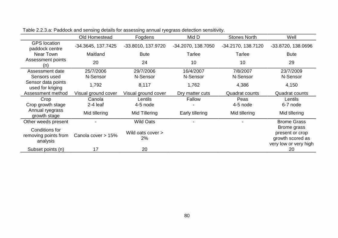
80

Table 2.2.3.a: Paddock and sensing details for assessing annual ryegrass detection sensitivity.

Old Homestead Fogdens Mid D Stones North Well

GPS location paddock centre

-34.3645, 137.7425 -33.8010, 137.9720 -34.2070, 138.7050 -34.2170, 138.7120 -33.8720, 138.0696

Near Town Maitland Bute Tarlee Tarlee Bute Assessment points

(n) 20 24 10 10 29

Assessment date 25/7/2006 29/7/2006 16/4/2007 7/8/2007 23/7/2009 Sensors used N-Sensor N-Sensor N-Sensor N-Sensor N-Sensor

Sensor data points used for kriging

1,792 8,117 1,762 4,386 4,150

Assessment method Visual ground cover Visual ground cover Dry matter cuts Quadrat counts Quadrat counts

Crop Canola Lentils Fallow Peas Lentils Crop growth stage 2-4 leaf 4-5 node - 4-5 node 6-7 node Annual ryegrass

growth stage Mid tillering Mid Tillering Early tillering Mid tillering Mid tillering

Other weeds present - Wild Oats - - Brome Grass

Conditions for removing points from

analysis Canola cover > 15%

Wild oats cover > 2%

Brome grass present or crop

growth scored as very low or very high

Subset points (n) 17 20 20

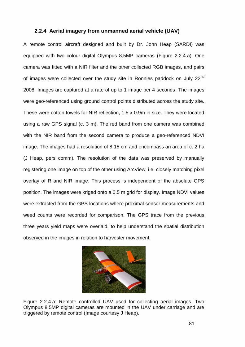
81

2.2.4 Aerial imagery from unmanned aerial vehicle (UAV)

A remote control aircraft designed and built by Dr. John Heap (SARDI) was

equipped with two colour digital Olympus 8.5MP cameras (Figure 2.2.4.a). One

camera was fitted with a NIR filter and the other collected RGB images, and pairs

of images were collected over the study site in Ronnies paddock on July 22nd

2008. Images are captured at a rate of up to 1 image per 4 seconds. The images

were geo-referenced using ground control points distributed across the study site.

These were cotton towels for NIR reflection, 1.5 x 0.9m in size. They were located

using a raw GPS signal (c. 3 m). The red band from one camera was combined

with the NIR band from the second camera to produce a geo-referenced NDVI

image. The images had a resolution of 8-15 cm and encompass an area of c. 2 ha

(J Heap, pers comm). The resolution of the data was preserved by manually

registering one image on top of the other using ArcView, i.e. closely matching pixel

overlay of R and NIR image. This process is independent of the absolute GPS

position. The images were kriged onto a 0.5 m grid for display. Image NDVI values

were extracted from the GPS locations where proximal sensor measurements and

weed counts were recorded for comparison. The GPS trace from the previous

three years yield maps were overlaid, to help understand the spatial distribution

observed in the images in relation to harvester movement.

Figure 2.2.4.a: Remote controlled UAV used for collecting aerial images. Two Olympus 8.5MP digital cameras are mounted in the UAV under carriage and are triggered by remote control (Image courtesy J Heap).

82

2.3 Results

2.3.1 Stationary sensor measurements

2.3.1.1 Optimised vegetative indices for annual ryegrass detection

Correlation coefficients between annual ryegrass density and specific wavebands

follow a similar trend to the reflectance signature of green plants (Figures 2.3.1.1.a

and 2.3.1.1.d). The measurements on the 4th of June in Ronnies paddock did not

follow this trend, as there was not enough green leaf area to affect the reflectance

(Figure 2.3.1.1.a). The points of greatest inflection in the visible region of the

spectrum occur at 550nm (green) and 670nm (red), while the NIR (750 – 900nm)

tends to have a strong positive correlation with annual ryegrass density. The

correlation coefficient trends down with growth stage, at both sites, except for 15th

June and 1st July in Ronnies paddock.

NDVI and SR indices were calculated using reflectance data from NIR (780nm),

blue (450nm), green (550nm) and red (670nm) wavelengths for comparison with

the biomass index (BI) calculated by the N-Sensor. These wavelengths were

selected as they showed the strongest positive and negative correlations with

annual ryegrass density or are significant points of inflection. NDVI, SR and BI

indices were then regressed with annual ryegrass density to determine the

coefficient of determination (R2) when a natural log curve was fitted. In Ronnies

paddock the coefficient of determination ranged from 0.08 to 0.67 and were in

general lower than the coefficient of determinations achieved in Stones South

paddock, where they range from 0.48 to 0.83 (Figure 2.3.1.1.b and 2.3.1.1.e). At

both sites the coefficient of determination was greater for NDVI than SR for all

dates when calculated using the same wavelengths. On the first sensing date at

83

both sites, the NDVI (red) calculated using red and NIR reflectance had the higher

coefficient of determination, however at the later sensing dates the NDVI (green)

calculated using the green reflectance data had higher coefficient of determination,

except the NDVI (blue) was marginally better in Stones South on two dates.

Despite the R2 values, that indicate the indices calculated using blue and green

wavelength reflectance can fit the data as well as the indices calculated using red

reflectance, the trend is always for a greater slope for the indices using red

reflectance, whether it be NDVI (red) or SR (red) (Figure 2.3.1.1.c, 2.3.1.1.f). This

suggests the indices using red reflectance will be better able to discriminate

annual ryegrass density, particularly at the lower population densities.

At the two earliest sensing dates in Ronnies and Stones South paddock the NDVI

(red) has a steeper slope than SR (red), at the third sensing date there is no

significant difference. At the fourth sensing SR (red) has the lowest R2, yet the

steepest slope (Figure 2.3.1.1.c, 2.3.1.1.f).

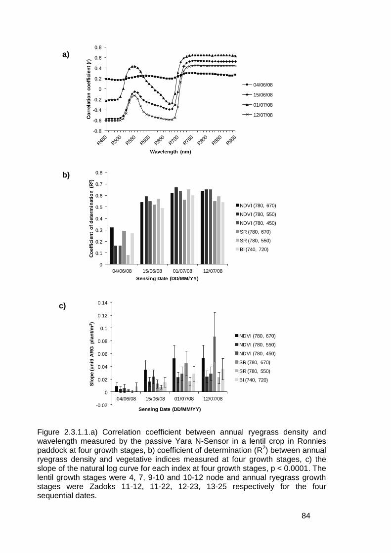
84

-0.8

-0.6

-0.4

-0.2

0

0.2

0.4

0.6

0.8

Co

rrela

tio

nco

eff

icie

nt

(r)

Wavelength (nm)

04/06/08

15/06/08

01/07/08

12/07/08

0

0.1

0.2

0.3

0.4

0.5

0.6

0.7

0.8

04/06/08 15/06/08 01/07/08 12/07/08

Co

eff

icie

nt

of

dete

rmin

ati

on

(R

2)

Sensing Date (DD/MM/YY)

NDVI (780, 670)

NDVI (780, 550)

NDVI (780, 450)

SR (780, 670)

SR (780, 550)

BI (740, 720)

-0.02

0

0.02

0.04

0.06

0.08

0.1

0.12

0.14

04/06/08 15/06/08 01/07/08 12/07/08

Slo

pe (u

nit

/ A

RG

pla

nt/

m2)

Sensing Date (DD/MM/YY)

NDVI (780, 670)

NDVI (780, 550)

NDVI (780, 450)

SR (780, 670)

SR (780, 550)

BI (740, 720)

Figure 2.3.1.1.a) Correlation coefficient between annual ryegrass density and wavelength measured by the passive Yara N-Sensor in a lentil crop in Ronnies paddock at four growth stages, b) coefficient of determination (R2) between annual ryegrass density and vegetative indices measured at four growth stages, c) the slope of the natural log curve for each index at four growth stages, p < 0.0001. The lentil growth stages were 4, 7, 9-10 and 10-12 node and annual ryegrass growth stages were Zadoks 11-12, 11-22, 12-23, 13-25 respectively for the four sequential dates.

a)

c)

b)

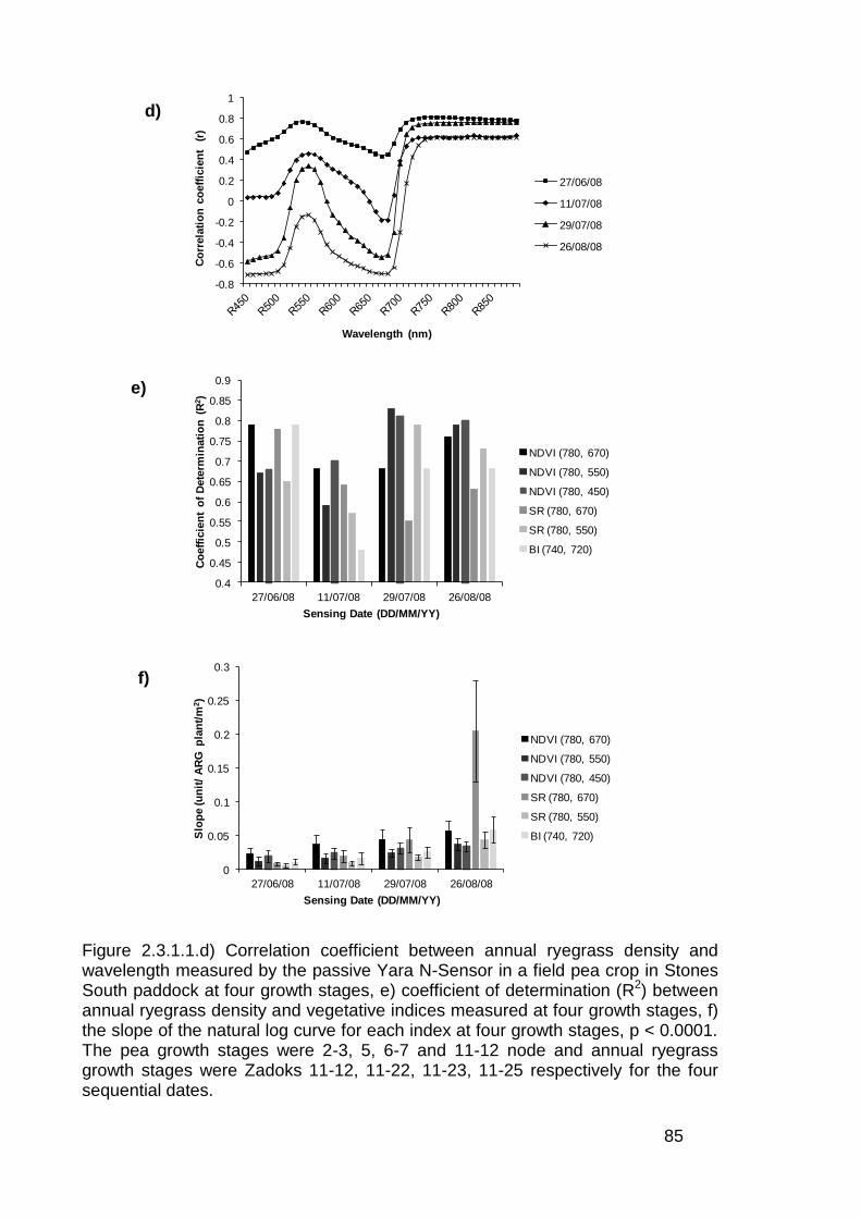
85

-0.8

-0.6

-0.4

-0.2

0

0.2

0.4

0.6

0.8

1

Co

rrela

tio

n c

oeff

icie

nt

(r)

Wavelength (nm)

27/06/08

11/07/08

29/07/08

26/08/08

0.4

0.45

0.5

0.55

0.6

0.65

0.7

0.75

0.8

0.85

0.9

27/06/08 11/07/08 29/07/08 26/08/08

Co

eff

icie

nt

of

Dete

rmin

ati

on

(R

2)

Sensing Date (DD/MM/YY)

NDVI (780, 670)

NDVI (780, 550)

NDVI (780, 450)

SR (780, 670)

SR (780, 550)

BI (740, 720)

0

0.05

0.1

0.15

0.2

0.25

0.3

27/06/08 11/07/08 29/07/08 26/08/08

Slo

pe (u

nit

/ A

RG

pla

nt/

m2)

Sensing Date (DD/MM/YY)

NDVI (780, 670)

NDVI (780, 550)

NDVI (780, 450)

SR (780, 670)

SR (780, 550)

BI (740, 720)

Figure 2.3.1.1.d) Correlation coefficient between annual ryegrass density and wavelength measured by the passive Yara N-Sensor in a field pea crop in Stones South paddock at four growth stages, e) coefficient of determination (R2) between annual ryegrass density and vegetative indices measured at four growth stages, f) the slope of the natural log curve for each index at four growth stages, p < 0.0001. The pea growth stages were 2-3, 5, 6-7 and 11-12 node and annual ryegrass growth stages were Zadoks 11-12, 11-22, 11-23, 11-25 respectively for the four sequential dates.

d)

f)

e)

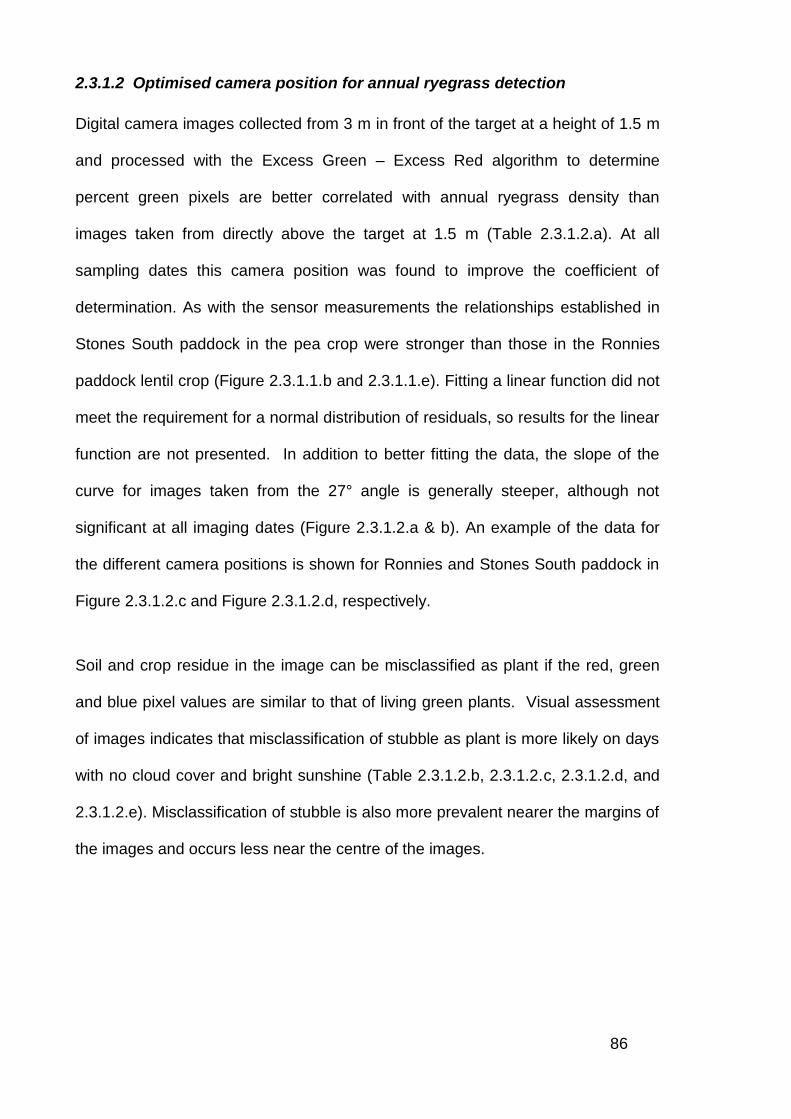
86

2.3.1.2 Optimised camera position for annual ryegrass detection

Digital camera images collected from 3 m in front of the target at a height of 1.5 m

and processed with the Excess Green – Excess Red algorithm to determine

percent green pixels are better correlated with annual ryegrass density than

images taken from directly above the target at 1.5 m (Table 2.3.1.2.a). At all

sampling dates this camera position was found to improve the coefficient of

determination. As with the sensor measurements the relationships established in

Stones South paddock in the pea crop were stronger than those in the Ronnies

paddock lentil crop (Figure 2.3.1.1.b and 2.3.1.1.e). Fitting a linear function did not

meet the requirement for a normal distribution of residuals, so results for the linear

function are not presented. In addition to better fitting the data, the slope of the

curve for images taken from the 27° angle is generally steeper, although not

significant at all imaging dates (Figure 2.3.1.2.a & b). An example of the data for

the different camera positions is shown for Ronnies and Stones South paddock in

Figure 2.3.1.2.c and Figure 2.3.1.2.d, respectively.

Soil and crop residue in the image can be misclassified as plant if the red, green

and blue pixel values are similar to that of living green plants. Visual assessment

of images indicates that misclassification of stubble as plant is more likely on days

with no cloud cover and bright sunshine (Table 2.3.1.2.b, 2.3.1.2.c, 2.3.1.2.d, and

2.3.1.2.e). Misclassification of stubble is also more prevalent nearer the margins of

the images and occurs less near the centre of the images.

87

Table 2.3.1.2.a: The relationship strength between annual ryegrass density and the ExG – ExR algorithm with the digital camera positioned 1.5 m directly above the target or 3 m in front and 1.5 m high (27˚ angle above soil level). Natural log curves have been fitted and the coefficient of determination (R2) represents the relationship strength.

Paddock Camera Position

Timing 1 Timing 2 Timing 3 Timing 4

Ronnies

Directly above

0.06 0.69 0.59 0.46

27˚ Angle

0.14 0.68 0.68 0.78

Stones Sth

Directly above

0.51 0.62 0.65 0.66

27˚ Angle

0.72 0.7 0.67 0.82

-2

0

2

4

6

8

10

12

14

16

04/06/08 15/06/08 01/07/08 12/07/08

Slo

pe (u

nit

/ A

RG

pla

nt/

m2)

Sensing Date (DD/MM/YY)

Directly above

27 angle

0

2

4

6

8

10

12

14

27/06/08 11/07/08 29/07/08 26/08/08

Slo

pe (u

nit

/ A

RG

pla

nt/

m2)

Sensing Date (DD/MM/YY)

Directly above

27 angle

Figure 2.3.1.2.a) the slope of the natural log curve between annual ryegrass density and percent plant pixels for four sampling dates and two camera positions for a) Ronnies paddock (p < 0.0001) and b) Stones South paddock (p < 0.0001).

b)

a)

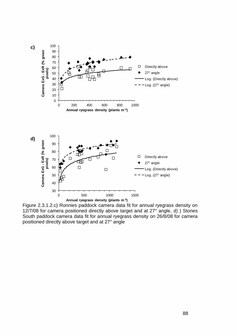
88

0

10

20

30

40

50

60

70

80

90

100

0 200 400 600 800 1000

Cam

era

ExG

-E

xR

(%

gre

en

p

ixels

)

Annual ryegrass density (plants m-2)

Directly above

27° angle

Log. (Directly above)

Log. (27° angle)

30

40

50

60

70

80

90

100

0 500 1000 1500

Cam

era

ExG

-E

xR

(%

gre

en

p

ixels

)

Annual ryegrass density (plants m-2)

Directly above

27° angle

Log. (Directly above)

Log. (27° angle)

Figure 2.3.1.2.c) Ronnies paddock camera data fit for annual ryegrass density on 12/7/08 for camera positioned directly above target and at 27° angle, d) ) Stones South paddock camera data fit for annual ryegrass density on 26/8/08 for camera positioned directly above target and at 27° angle

d)

c)

89

Table 2.3.1.2.b: Example RGB images and the corresponding classified binary image for four imaging dates at a low annual ryegrass density site (10 plants m-2) in lentils in Ronnies paddock.

Timing 04/06/08 15/06/08 01/07/08 12/07/08

Cloud Cover (%) 70 0 70 80

Greenseeker NDVI 0.166 0.181 0.309 0.355

Camera position directly above target: RGB image and binary classified image

ExG – ExR Cover (%) 1.9 8.61 20.44 22.92

Camera positioned 3m in front and 1.5m high (27˚ angle above soil level): RGB image and binary classified image

ExG – ExR Cover (%) 3.3 12.96 22.93 29.68

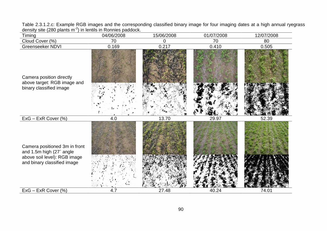
90

Table 2.3.1.2.c: Example RGB images and the corresponding classified binary image for four imaging dates at a high annual ryegrass density site (280 plants m-2) in lentils in Ronnies paddock.

Timing 04/06/2008 15/06/2008 01/07/2008 12/07/2008

Cloud Cover (%) 70 0 70 80

Greenseeker NDVI 0.169 0.217 0.410 0.505

Camera position directly above target: RGB image and binary classified image

ExG – ExR Cover (%) 4.0 13.70 29.97 52.39

Camera positioned 3m in front and 1.5m high (27˚ angle above soil level): RGB image and binary classified image

ExG – ExR Cover (%) 4.7 27.48 40.24 74.01

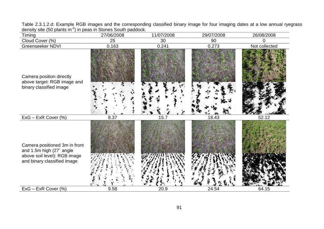
91

Table 2.3.1.2.d: Example RGB images and the corresponding classified binary image for four imaging dates at a low annual ryegrass density site (50 plants m-2) in peas in Stones South paddock.

Timing 27/06/2008 11/07/2008 29/07/2008 26/08/2008

Cloud Cover (%) 25 30 90 0

Greenseeker NDVI 0.163 0.241 0.273 Not collected

Camera position directly above target: RGB image and binary classified image

ExG – ExR Cover (%) 8.37 15.7 18.43 52.12

Camera positioned 3m in front and 1.5m high (27˚ angle above soil level): RGB image and binary classified image

ExG – ExR Cover (%) 9.58 20.9 24.54 64.15

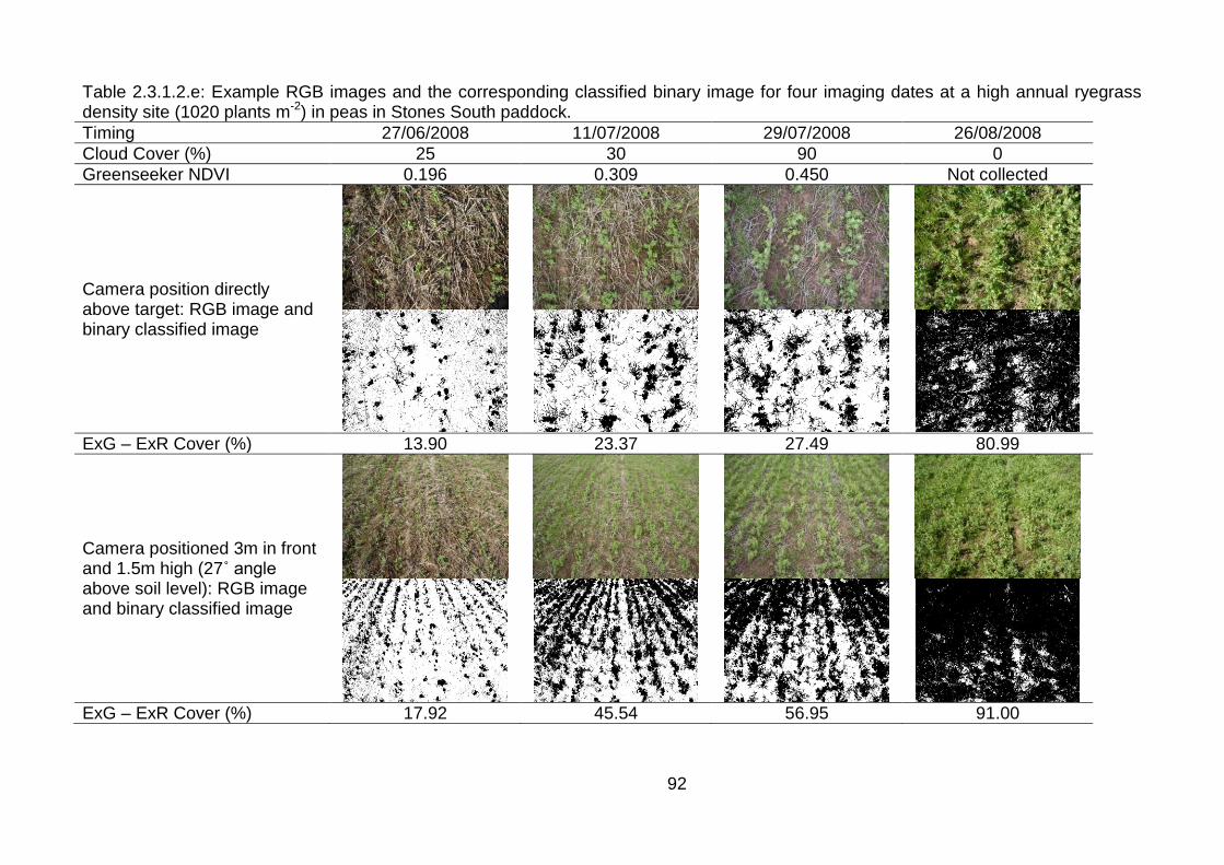
92

Table 2.3.1.2.e: Example RGB images and the corresponding classified binary image for four imaging dates at a high annual ryegrass density site (1020 plants m-2) in peas in Stones South paddock.

Timing 27/06/2008 11/07/2008 29/07/2008 26/08/2008

Cloud Cover (%) 25 30 90 0

Greenseeker NDVI 0.196 0.309 0.450 Not collected

Camera position directly above target: RGB image and binary classified image

ExG – ExR Cover (%) 13.90 23.37 27.49 80.99

Camera positioned 3m in front and 1.5m high (27˚ angle above soil level): RGB image and binary classified image

ExG – ExR Cover (%) 17.92 45.54 56.95 91.00

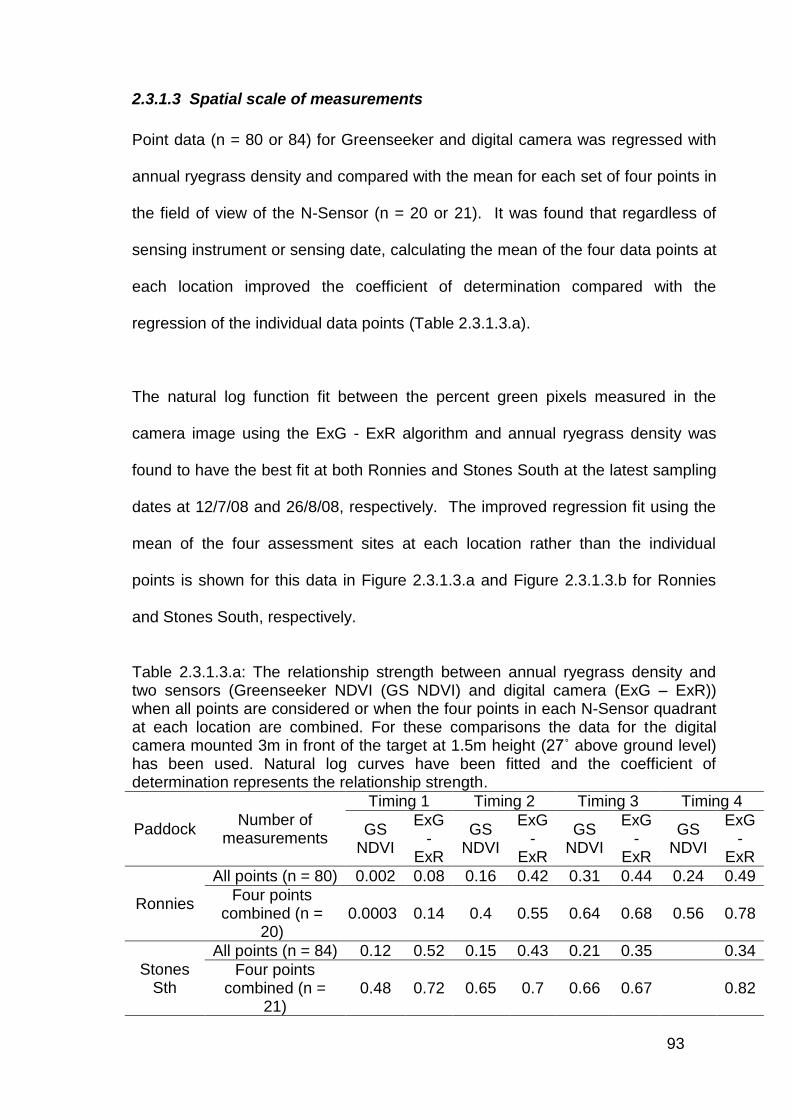
93

2.3.1.3 Spatial scale of measurements

Point data (n = 80 or 84) for Greenseeker and digital camera was regressed with

annual ryegrass density and compared with the mean for each set of four points in

the field of view of the N-Sensor (n = 20 or 21). It was found that regardless of

sensing instrument or sensing date, calculating the mean of the four data points at

each location improved the coefficient of determination compared with the

regression of the individual data points (Table 2.3.1.3.a).

The natural log function fit between the percent green pixels measured in the

camera image using the ExG - ExR algorithm and annual ryegrass density was

found to have the best fit at both Ronnies and Stones South at the latest sampling

dates at 12/7/08 and 26/8/08, respectively. The improved regression fit using the

mean of the four assessment sites at each location rather than the individual

points is shown for this data in Figure 2.3.1.3.a and Figure 2.3.1.3.b for Ronnies

and Stones South, respectively.

Table 2.3.1.3.a: The relationship strength between annual ryegrass density and two sensors (Greenseeker NDVI (GS NDVI) and digital camera (ExG – ExR)) when all points are considered or when the four points in each N-Sensor quadrant at each location are combined. For these comparisons the data for the digital camera mounted 3m in front of the target at 1.5m height (27˚ above ground level) has been used. Natural log curves have been fitted and the coefficient of determination represents the relationship strength.

Paddock Number of

measurements

Timing 1 Timing 2 Timing 3 Timing 4

GS NDVI

ExG -

ExR

GS NDVI

ExG -

ExR

GS NDVI

ExG -

ExR

GS NDVI

ExG -

ExR

Ronnies

All points (n = 80) 0.002 0.08 0.16 0.42 0.31 0.44 0.24 0.49

Four points combined (n =

20) 0.0003 0.14 0.4 0.55 0.64 0.68 0.56 0.78

Stones Sth

All points (n = 84) 0.12 0.52 0.15 0.43 0.21 0.35 0.34

Four points combined (n =

21) 0.48 0.72 0.65 0.7 0.66 0.67 0.82

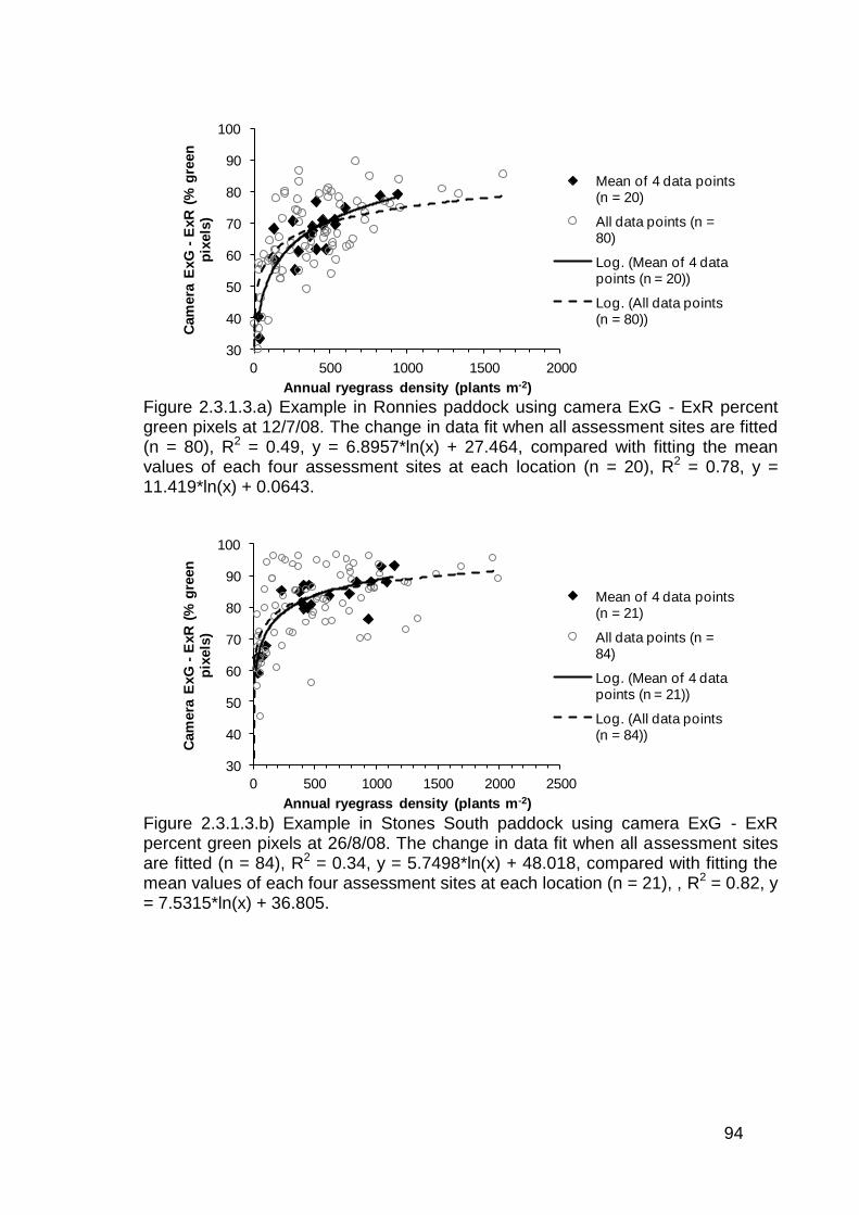
94

30

40

50

60

70

80

90

100

0 500 1000 1500 2000

Cam

era

ExG

-E

xR

(%

gre

en

p

ixels

)

Annual ryegrass density (plants m-2)

Mean of 4 data points (n = 20)

All data points (n = 80)

Log. (Mean of 4 data points (n = 20))

Log. (All data points (n = 80))

Figure 2.3.1.3.a) Example in Ronnies paddock using camera ExG - ExR percent green pixels at 12/7/08. The change in data fit when all assessment sites are fitted (n = 80), R2 = 0.49, y = 6.8957*ln(x) + 27.464, compared with fitting the mean values of each four assessment sites at each location (n = 20), R2 = 0.78, y = 11.419*ln(x) + 0.0643.

30

40

50

60

70

80

90

100

0 500 1000 1500 2000 2500

Cam

era

ExG

-E

xR

(%

gre

en

p

ixels

)

Annual ryegrass density (plants m-2)

Mean of 4 data points (n = 21)

All data points (n = 84)

Log. (Mean of 4 data points (n = 21))

Log. (All data points (n = 84))

Figure 2.3.1.3.b) Example in Stones South paddock using camera ExG - ExR percent green pixels at 26/8/08. The change in data fit when all assessment sites are fitted (n = 84), R2 = 0.34, y = 5.7498*ln(x) + 48.018, compared with fitting the mean values of each four assessment sites at each location (n = 21), , R2 = 0.82, y = 7.5315*ln(x) + 36.805.

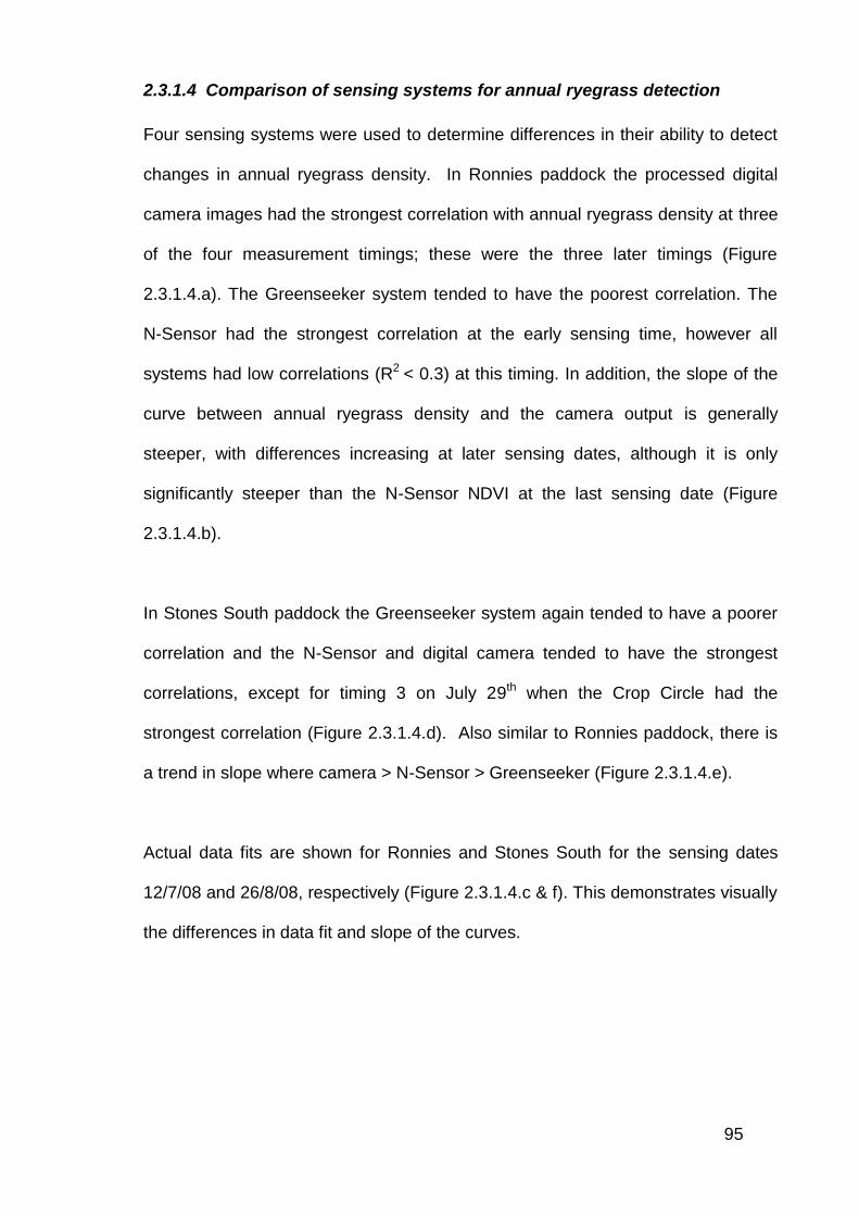
95

2.3.1.4 Comparison of sensing systems for annual ryegrass detection

Four sensing systems were used to determine differences in their ability to detect

changes in annual ryegrass density. In Ronnies paddock the processed digital

camera images had the strongest correlation with annual ryegrass density at three

of the four measurement timings; these were the three later timings (Figure

2.3.1.4.a). The Greenseeker system tended to have the poorest correlation. The

N-Sensor had the strongest correlation at the early sensing time, however all

systems had low correlations (R2 < 0.3) at this timing. In addition, the slope of the

curve between annual ryegrass density and the camera output is generally

steeper, with differences increasing at later sensing dates, although it is only

significantly steeper than the N-Sensor NDVI at the last sensing date (Figure

2.3.1.4.b).

In Stones South paddock the Greenseeker system again tended to have a poorer

correlation and the N-Sensor and digital camera tended to have the strongest

correlations, except for timing 3 on July 29th when the Crop Circle had the

strongest correlation (Figure 2.3.1.4.d). Also similar to Ronnies paddock, there is

a trend in slope where camera > N-Sensor > Greenseeker (Figure 2.3.1.4.e).

Actual data fits are shown for Ronnies and Stones South for the sensing dates

12/7/08 and 26/8/08, respectively (Figure 2.3.1.4.c & f). This demonstrates visually

the differences in data fit and slope of the curves.

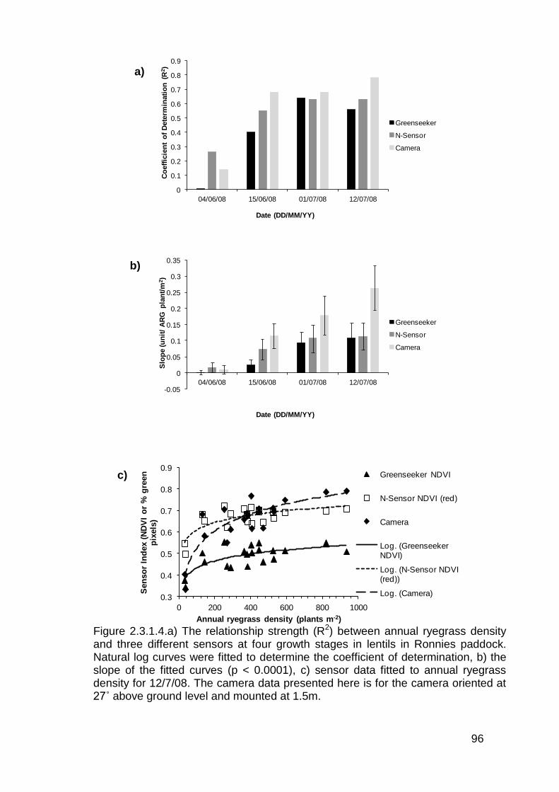
96

0

0.1

0.2

0.3

0.4

0.5

0.6

0.7

0.8

0.9

04/06/08 15/06/08 01/07/08 12/07/08

Co

eff

icie

nt

of

Dete

rmin

ati

on

(R

2)

Date (DD/MM/YY)

Greenseeker

N-Sensor

Camera

-0.05

0

0.05

0.1

0.15

0.2

0.25

0.3

0.35

04/06/08 15/06/08 01/07/08 12/07/08

Slo

pe (u

nit

/ A

RG

pla

nt/

m2)

Date (DD/MM/YY)

Greenseeker

N-Sensor

Camera

0.3

0.4

0.5

0.6

0.7

0.8

0.9

0 200 400 600 800 1000

Sen

so

r In

dex (

ND

VI

or

% g

reen

p

ixels

)

Annual ryegrass density (plants m-2)

Greenseeker NDVI

N-Sensor NDVI (red)

Camera

Log. (Greenseeker NDVI)

Log. (N-Sensor NDVI (red))

Log. (Camera)

Figure 2.3.1.4.a) The relationship strength (R2) between annual ryegrass density and three different sensors at four growth stages in lentils in Ronnies paddock. Natural log curves were fitted to determine the coefficient of determination, b) the slope of the fitted curves (p < 0.0001), c) sensor data fitted to annual ryegrass density for 12/7/08. The camera data presented here is for the camera oriented at 27˚ above ground level and mounted at 1.5m.

a)

b)

c)

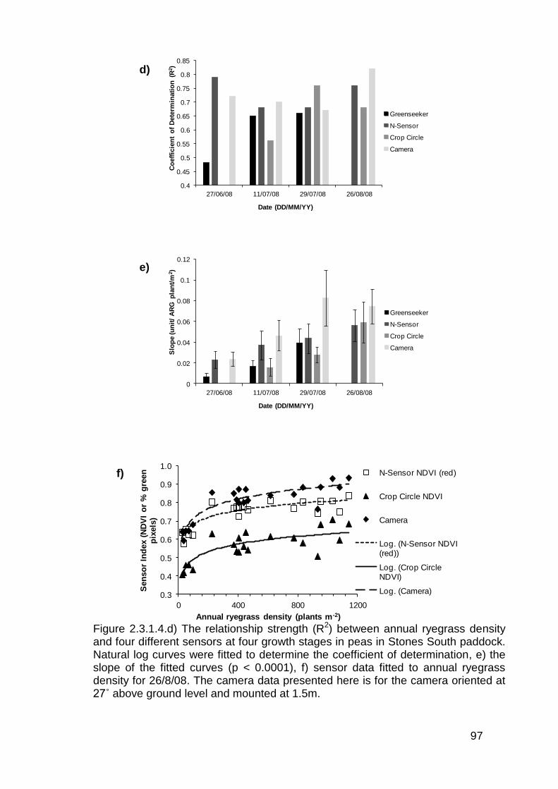
97

0.4

0.45

0.5

0.55

0.6

0.65

0.7

0.75

0.8

0.85

27/06/08 11/07/08 29/07/08 26/08/08

Co

eff

icie

nt

of

Dete

rmin

ati

on

(R

2)

Date (DD/MM/YY)

Greenseeker

N-Sensor

Crop Circle

Camera

0

0.02

0.04

0.06

0.08

0.1

0.12

27/06/08 11/07/08 29/07/08 26/08/08

Slo

pe (u

nit

/ A

RG

pla

nt/

m2)

Date (DD/MM/YY)

Greenseeker

N-Sensor

Crop Circle

Camera

0.3

0.4

0.5

0.6

0.7

0.8

0.9

1.0

0 400 800 1200

Sen

so

r In

dex (

ND

VI

or

% g

reen

p

ixels

)

Annual ryegrass density (plants m-2)

N-Sensor NDVI (red)

Crop Circle NDVI

Camera

Log. (N-Sensor NDVI (red))

Log. (Crop Circle NDVI)

Log. (Camera)

Figure 2.3.1.4.d) The relationship strength (R2) between annual ryegrass density and four different sensors at four growth stages in peas in Stones South paddock. Natural log curves were fitted to determine the coefficient of determination, e) the slope of the fitted curves (p < 0.0001), f) sensor data fitted to annual ryegrass density for 26/8/08. The camera data presented here is for the camera oriented at 27˚ above ground level and mounted at 1.5m.

e)

d)

f)

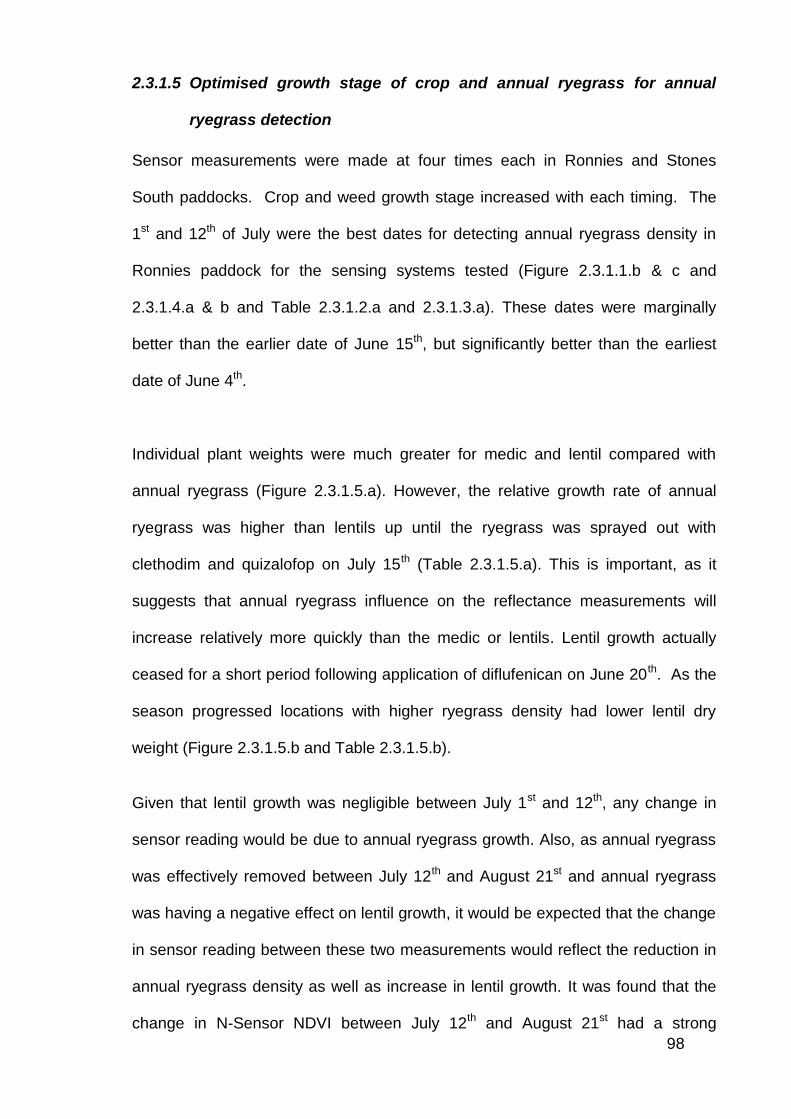
98

2.3.1.5 Optimised growth stage of crop and annual ryegrass for annual

ryegrass detection

Sensor measurements were made at four times each in Ronnies and Stones

South paddocks. Crop and weed growth stage increased with each timing. The

1st and 12th of July were the best dates for detecting annual ryegrass density in

Ronnies paddock for the sensing systems tested (Figure 2.3.1.1.b & c and

2.3.1.4.a & b and Table 2.3.1.2.a and 2.3.1.3.a). These dates were marginally

better than the earlier date of June 15th, but significantly better than the earliest

date of June 4th.

Individual plant weights were much greater for medic and lentil compared with

annual ryegrass (Figure 2.3.1.5.a). However, the relative growth rate of annual

ryegrass was higher than lentils up until the ryegrass was sprayed out with

clethodim and quizalofop on July 15th (Table 2.3.1.5.a). This is important, as it

suggests that annual ryegrass influence on the reflectance measurements will

increase relatively more quickly than the medic or lentils. Lentil growth actually

ceased for a short period following application of diflufenican on June 20th. As the

season progressed locations with higher ryegrass density had lower lentil dry

weight (Figure 2.3.1.5.b and Table 2.3.1.5.b).

Given that lentil growth was negligible between July 1st and 12th, any change in

sensor reading would be due to annual ryegrass growth. Also, as annual ryegrass

was effectively removed between July 12th and August 21st and annual ryegrass

was having a negative effect on lentil growth, it would be expected that the change

in sensor reading between these two measurements would reflect the reduction in

annual ryegrass density as well as increase in lentil growth. It was found that the

change in N-Sensor NDVI between July 12th and August 21st had a strong

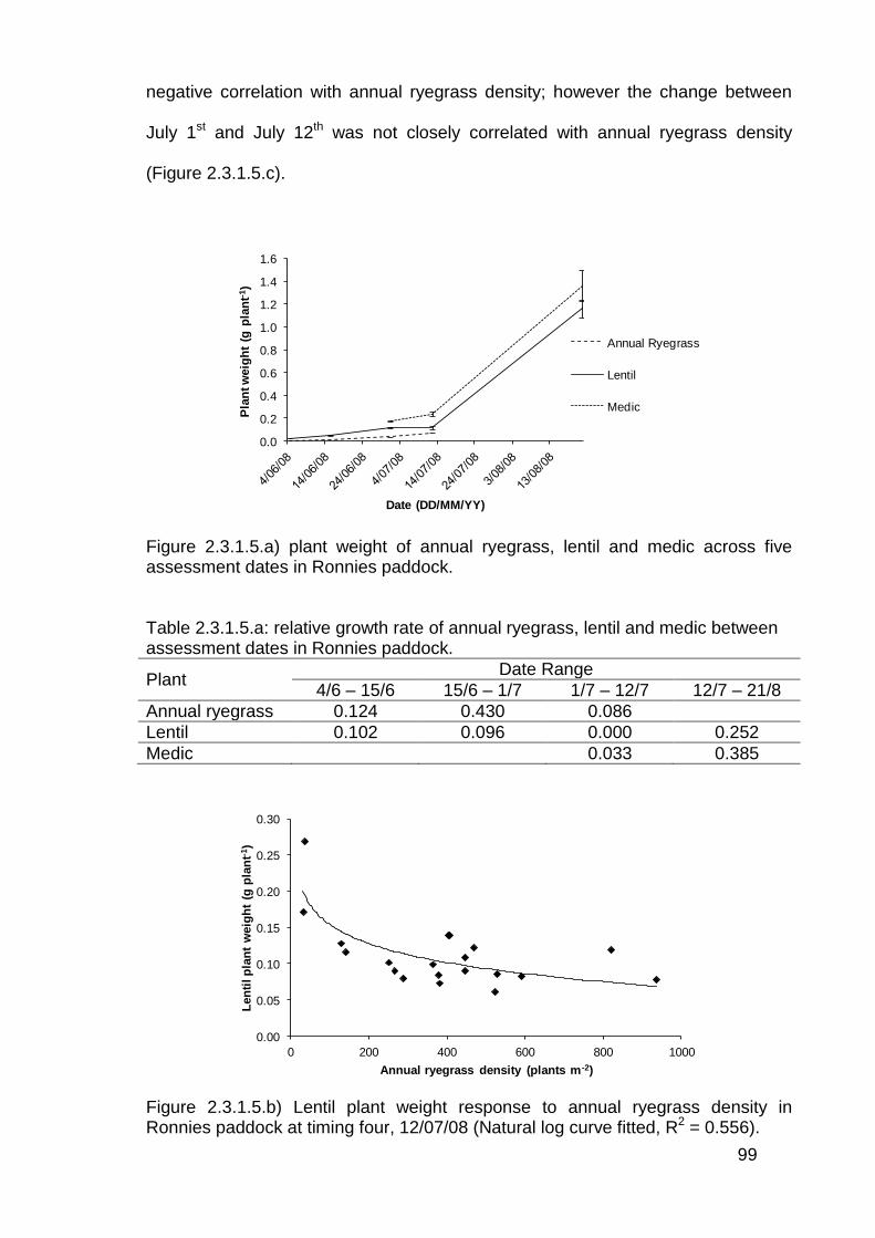
99

negative correlation with annual ryegrass density; however the change between

July 1st and July 12th was not closely correlated with annual ryegrass density

(Figure 2.3.1.5.c).

0.0

0.2

0.4

0.6

0.8

1.0

1.2

1.4

1.6

Pla

nt w

eig

ht

(g p

lan

t-1)

Date (DD/MM/YY)

Annual Ryegrass

Lentil

Medic

Figure 2.3.1.5.a) plant weight of annual ryegrass, lentil and medic across five assessment dates in Ronnies paddock. Table 2.3.1.5.a: relative growth rate of annual ryegrass, lentil and medic between assessment dates in Ronnies paddock.

Plant Date Range

4/6 – 15/6 15/6 – 1/7 1/7 – 12/7 12/7 – 21/8

Annual ryegrass 0.124 0.430 0.086

Lentil 0.102 0.096 0.000 0.252

Medic 0.033 0.385

0.00

0.05

0.10

0.15

0.20

0.25

0.30

0 200 400 600 800 1000

Len

til p

lan

t w

eig

ht

(g p

lan

t-1)

Annual ryegrass density (plants m-2)

Figure 2.3.1.5.b) Lentil plant weight response to annual ryegrass density in Ronnies paddock at timing four, 12/07/08 (Natural log curve fitted, R2 = 0.556).

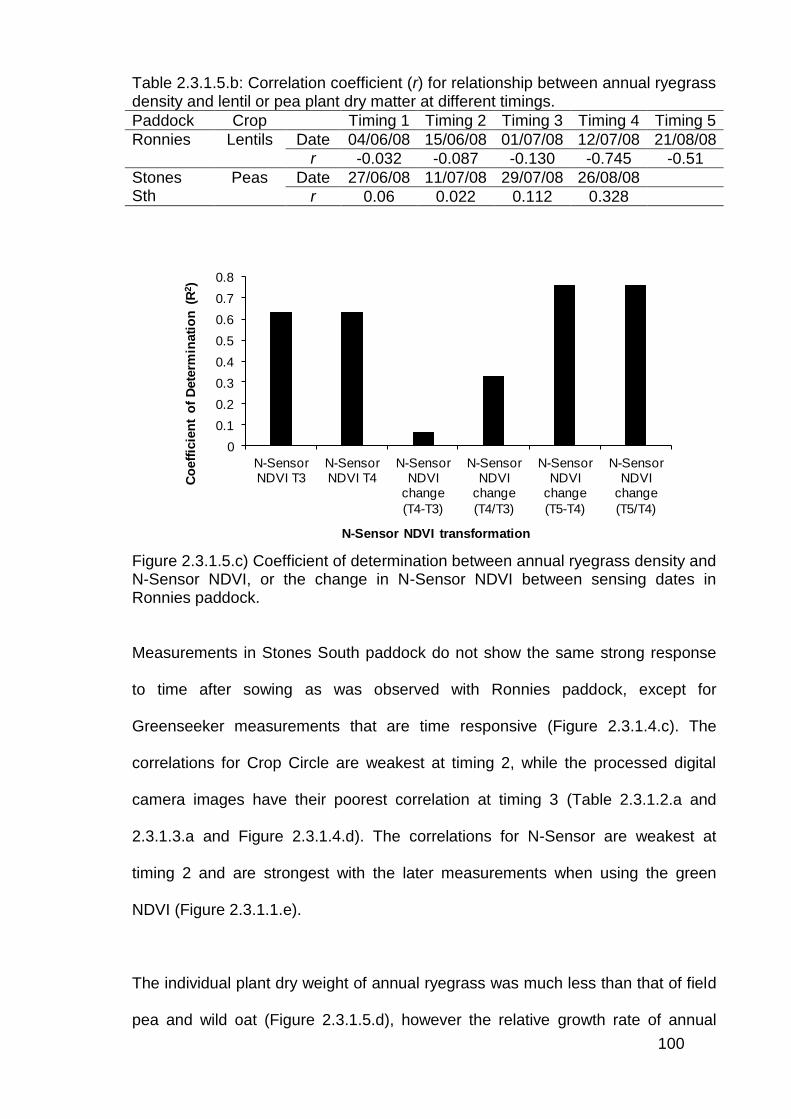
100

Table 2.3.1.5.b: Correlation coefficient (r) for relationship between annual ryegrass density and lentil or pea plant dry matter at different timings.

Paddock Crop Timing 1 Timing 2 Timing 3 Timing 4 Timing 5

Ronnies Lentils Date 04/06/08 15/06/08 01/07/08 12/07/08 21/08/08

r -0.032 -0.087 -0.130 -0.745 -0.51

Stones Sth

Peas Date 27/06/08 11/07/08 29/07/08 26/08/08

r 0.06 0.022 0.112 0.328

0

0.1

0.2

0.3

0.4

0.5

0.6

0.7

0.8

N-Sensor NDVI T3

N-Sensor NDVI T4

N-Sensor NDVI

change

(T4-T3)

N-Sensor NDVI

change

(T4/T3)

N-Sensor NDVI

change

(T5-T4)

N-Sensor NDVI

change

(T5/T4)

Co

eff

icie

nt

of

Dete

rmin

ati

on

(R

2)

N-Sensor NDVI transformation

Figure 2.3.1.5.c) Coefficient of determination between annual ryegrass density and N-Sensor NDVI, or the change in N-Sensor NDVI between sensing dates in Ronnies paddock.

Measurements in Stones South paddock do not show the same strong response

to time after sowing as was observed with Ronnies paddock, except for

Greenseeker measurements that are time responsive (Figure 2.3.1.4.c). The

correlations for Crop Circle are weakest at timing 2, while the processed digital

camera images have their poorest correlation at timing 3 (Table 2.3.1.2.a and

2.3.1.3.a and Figure 2.3.1.4.d). The correlations for N-Sensor are weakest at

timing 2 and are strongest with the later measurements when using the green

NDVI (Figure 2.3.1.1.e).

The individual plant dry weight of annual ryegrass was much less than that of field

pea and wild oat (Figure 2.3.1.5.d), however the relative growth rate of annual

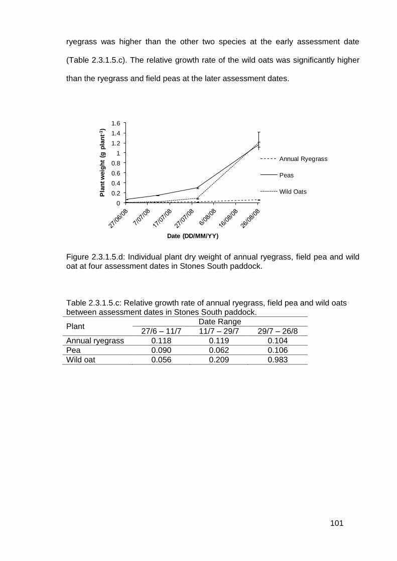
101

ryegrass was higher than the other two species at the early assessment date

(Table 2.3.1.5.c). The relative growth rate of the wild oats was significantly higher

than the ryegrass and field peas at the later assessment dates.

0

0.2

0.4

0.6

0.8

1

1.2

1.4

1.6

Pla

nt w

eig

ht

(g p

lan

t-1)

Date (DD/MM/YY)

Annual Ryegrass

Peas

Wild Oats

Figure 2.3.1.5.d: Individual plant dry weight of annual ryegrass, field pea and wild oat at four assessment dates in Stones South paddock. Table 2.3.1.5.c: Relative growth rate of annual ryegrass, field pea and wild oats between assessment dates in Stones South paddock.

Plant Date Range

27/6 – 11/7 11/7 – 29/7 29/7 – 26/8

Annual ryegrass 0.118 0.119 0.104

Pea 0.090 0.062 0.106

Wild oat 0.056 0.209 0.983

102

2.3.1.6 Optimised relationships between sensing systems and crop and

weed measurements

Snail medic and wild oat densities varied across Ronnies and Stones South,

respectively. Assessments were made to determine what effect their presence

had on detection of changes in annual ryegrass density. Calculating the summed

dry matter of annual ryegrass and snail medic for regression with the sensor

measurements improved the correlations for both sensors in Ronnies paddock

(Figure 2.3.1.6.a). Excluding locations with more than 20 snail medic plants m-2

from the analysis improved the correlations even further.

Calculating the summed dry matter of annual ryegrass and wild oats for regression

with the sensor measurements improved the correlation for both sensors at one

measurement time only and significantly reduced the correlations at the other

measurement times (Figure 2.3.1.6.b). However, excluding locations with more

than 10 wild oat plants m-2 from the analysis improved the correlations for all

sensors at all assessment dates.

The best data fits were between annual ryegrass density and camera ExG - ExR

percent green pixels measured at the latest timing in both paddocks. This was

improved slightly when adjusted for medic and wild oat density in Ronnies and

Stones South, respectively (Figure 2.3.1.6.c & d). Whilst this adjustment improves

the coefficient of determination slightly, the shape and slope of the curve are

largely unchanged.

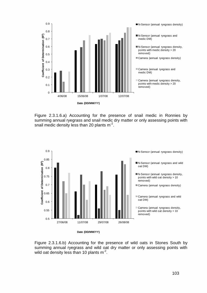
103

0

0.1

0.2

0.3

0.4

0.5

0.6

0.7

0.8

0.9

4/06/08 15/06/08 1/07/08 12/07/08

Co

eff

icie

nt

of

Dete

rmin

ati

on

(R

2)

Date (DD/MM/YY)

N-Sensor (annual ryegrass density)

N-Sensor (annual ryegrass and medic DM)

N-Sensor (annual ryegrass density, points with medic density > 20 removed)

Camera (annual ryegrass density)

Camera (annual ryegrass and medic DM)

Camera (annual ryegrass density, points with medic density > 20 removed)

Figure 2.3.1.6.a) Accounting for the presence of snail medic in Ronnies by summing annual ryegrass and snail medic dry matter or only assessing points with snail medic density less than 20 plants m-2.

0.5

0.55

0.6

0.65

0.7

0.75

0.8

0.85

0.9

27/06/08 11/07/08 29/07/08 26/08/08

Co

eff

icie

nt

of

Dete

rmin

ati

on

(R

2)

Date (DD/MM/YY)

N-Sensor (annual ryegrass density)

N-Sensor (annual ryegrass and wild oat DM)

N-Sensor (annual ryegrass density, points with wild oat density > 10 removed)

Camera (annual ryegrass density)

Camera (annual ryegrass and wild oat DM)

Camera (annual ryegrass density, points with wild oat density > 10 removed)

Figure 2.3.1.6.b) Accounting for the presence of wild oats in Stones South by summing annual ryegrass and wild oat dry matter or only assessing points with wild oat density less than 10 plants m-2.

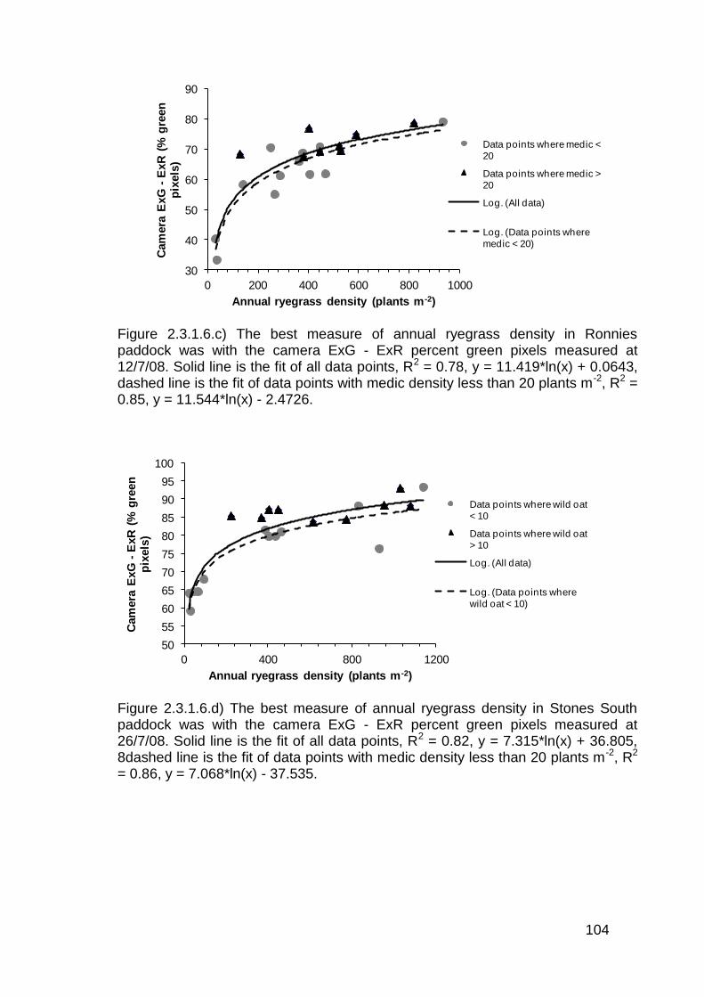
104

30

40

50

60

70

80

90

0 200 400 600 800 1000

Cam

era

ExG

-E

xR

(%

gre

en

p

ixels

)

Annual ryegrass density (plants m-2)

Data points where medic <

20

Data points where medic >

20

Log. (All data)

Log. (Data points where

medic < 20)

Figure 2.3.1.6.c) The best measure of annual ryegrass density in Ronnies paddock was with the camera ExG - ExR percent green pixels measured at 12/7/08. Solid line is the fit of all data points, R2 = 0.78, y = 11.419*ln(x) + 0.0643, dashed line is the fit of data points with medic density less than 20 plants m-2, R2 = 0.85, y = 11.544*ln(x) - 2.4726.

50

55

60

65

70

75

80

85

90

95

100

0 400 800 1200

Cam

era

ExG

-E

xR

(%

gre

en

p

ixels

)

Annual ryegrass density (plants m-2)

Data points where wild oat

< 10

Data points where wild oat

> 10

Log. (All data)

Log. (Data points where

wild oat < 10)

Figure 2.3.1.6.d) The best measure of annual ryegrass density in Stones South paddock was with the camera ExG - ExR percent green pixels measured at 26/7/08. Solid line is the fit of all data points, R2 = 0.82, y = 7.315*ln(x) + 36.805, 8dashed line is the fit of data points with medic density less than 20 plants m-2, R2 = 0.86, y = 7.068*ln(x) - 37.535.

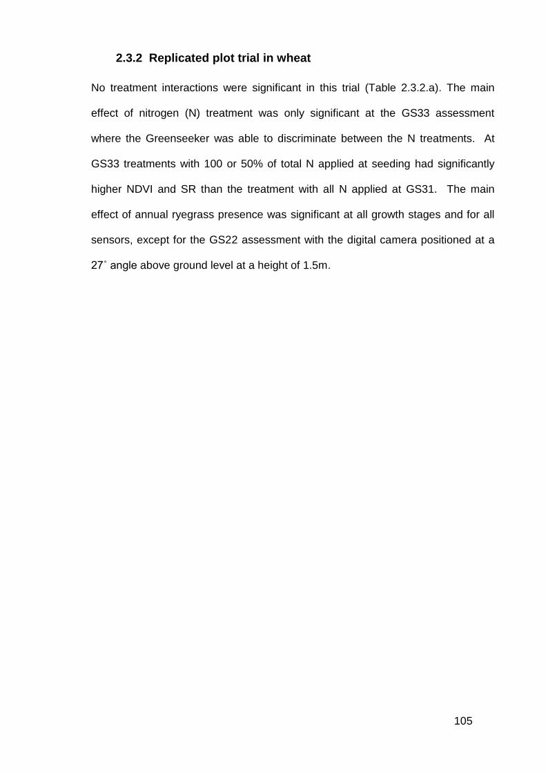
105

2.3.2 Replicated plot trial in wheat

No treatment interactions were significant in this trial (Table 2.3.2.a). The main

effect of nitrogen (N) treatment was only significant at the GS33 assessment

where the Greenseeker was able to discriminate between the N treatments. At

GS33 treatments with 100 or 50% of total N applied at seeding had significantly

higher NDVI and SR than the treatment with all N applied at GS31. The main

effect of annual ryegrass presence was significant at all growth stages and for all

sensors, except for the GS22 assessment with the digital camera positioned at a

27˚ angle above ground level at a height of 1.5m.

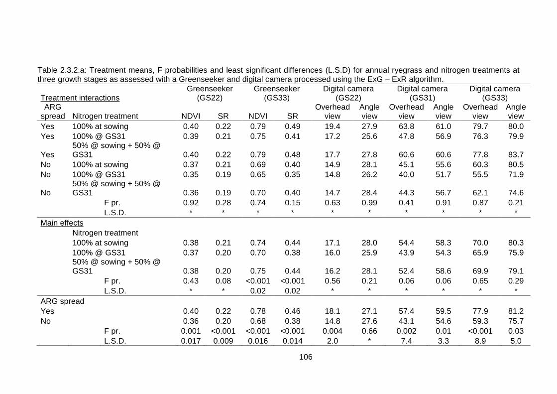
106

Table 2.3.2.a: Treatment means, F probabilities and least significant differences (L.S.D) for annual ryegrass and nitrogen treatments at three growth stages as assessed with a Greenseeker and digital camera processed using the ExG – ExR algorithm.

Treatment interactions Greenseeker

(GS22) Greenseeker

(GS33) Digital camera

(GS22) Digital camera

(GS31) Digital camera

(GS33) ARG

spread Nitrogen treatment NDVI SR NDVI SR Overhead

view Angle view

Overhead view

Angle view

Overhead view

Angle view

Yes 100% at sowing 0.40 0.22 0.79 0.49 19.4 27.9 63.8 61.0 79.7 80.0

Yes 100% @ GS31 0.39 0.21 0.75 0.41 17.2 25.6 47.8 56.9 76.3 79.9

Yes 50% @ sowing + 50% @ GS31 0.40 0.22 0.79 0.48 17.7 27.8 60.6 60.6 77.8 83.7

No 100% at sowing 0.37 0.21 0.69 0.40 14.9 28.1 45.1 55.6 60.3 80.5

No 100% @ GS31 0.35 0.19 0.65 0.35 14.8 26.2 40.0 51.7 55.5 71.9

No 50% @ sowing + 50% @ GS31 0.36 0.19 0.70 0.40 14.7 28.4 44.3 56.7 62.1 74.6

F pr. 0.92 0.28 0.74 0.15 0.63 0.99 0.41 0.91 0.87 0.21

L.S.D. * * * * * * * * * *

Main effects

Nitrogen treatment

100% at sowing 0.38 0.21 0.74 0.44 17.1 28.0 54.4 58.3 70.0 80.3

100% @ GS31 0.37 0.20 0.70 0.38 16.0 25.9 43.9 54.3 65.9 75.9

50% @ sowing + 50% @ GS31 0.38 0.20 0.75 0.44 16.2 28.1 52.4 58.6 69.9 79.1

F pr. 0.43 0.08 <0.001 <0.001 0.56 0.21 0.06 0.06 0.65 0.29

L.S.D. * * 0.02 0.02 * * * * * *

ARG spread Yes

0.40 0.22 0.78 0.46 18.1 27.1 57.4 59.5 77.9 81.2

No

0.36 0.20 0.68 0.38 14.8 27.6 43.1 54.6 59.3 75.7

F pr. 0.001 <0.001 <0.001 <0.001 0.004 0.66 0.002 0.01 <0.001 0.03

L.S.D. 0.017 0.009 0.016 0.014 2.0 * 7.4 3.3 8.9 5.0

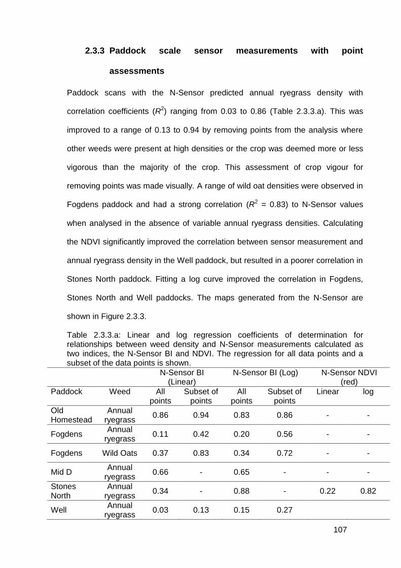
107

2.3.3 Paddock scale sensor measurements with point

assessments

Paddock scans with the N-Sensor predicted annual ryegrass density with

correlation coefficients (R2) ranging from 0.03 to 0.86 (Table 2.3.3.a). This was

improved to a range of 0.13 to 0.94 by removing points from the analysis where

other weeds were present at high densities or the crop was deemed more or less

vigorous than the majority of the crop. This assessment of crop vigour for

removing points was made visually. A range of wild oat densities were observed in

Fogdens paddock and had a strong correlation (R2 = 0.83) to N-Sensor values

when analysed in the absence of variable annual ryegrass densities. Calculating

the NDVI significantly improved the correlation between sensor measurement and

annual ryegrass density in the Well paddock, but resulted in a poorer correlation in

Stones North paddock. Fitting a log curve improved the correlation in Fogdens,

Stones North and Well paddocks. The maps generated from the N-Sensor are

shown in Figure 2.3.3.

Table 2.3.3.a: Linear and log regression coefficients of determination for relationships between weed density and N-Sensor measurements calculated as two indices, the N-Sensor BI and NDVI. The regression for all data points and a subset of the data points is shown.

N-Sensor BI (Linear)

N-Sensor BI (Log) N-Sensor NDVI (red)

Paddock Weed All points

Subset of points

All points

Subset of points

Linear log

Old Homestead

Annual ryegrass

0.86 0.94 0.83 0.86 - -

Fogdens Annual

ryegrass 0.11 0.42 0.20 0.56 - -

Fogdens Wild Oats 0.37 0.83 0.34 0.72 - -

Mid D Annual

ryegrass 0.66 - 0.65 - - -

Stones North

Annual ryegrass

0.34 - 0.88 - 0.22 0.82

Well Annual

ryegrass 0.03 0.13 0.15 0.27

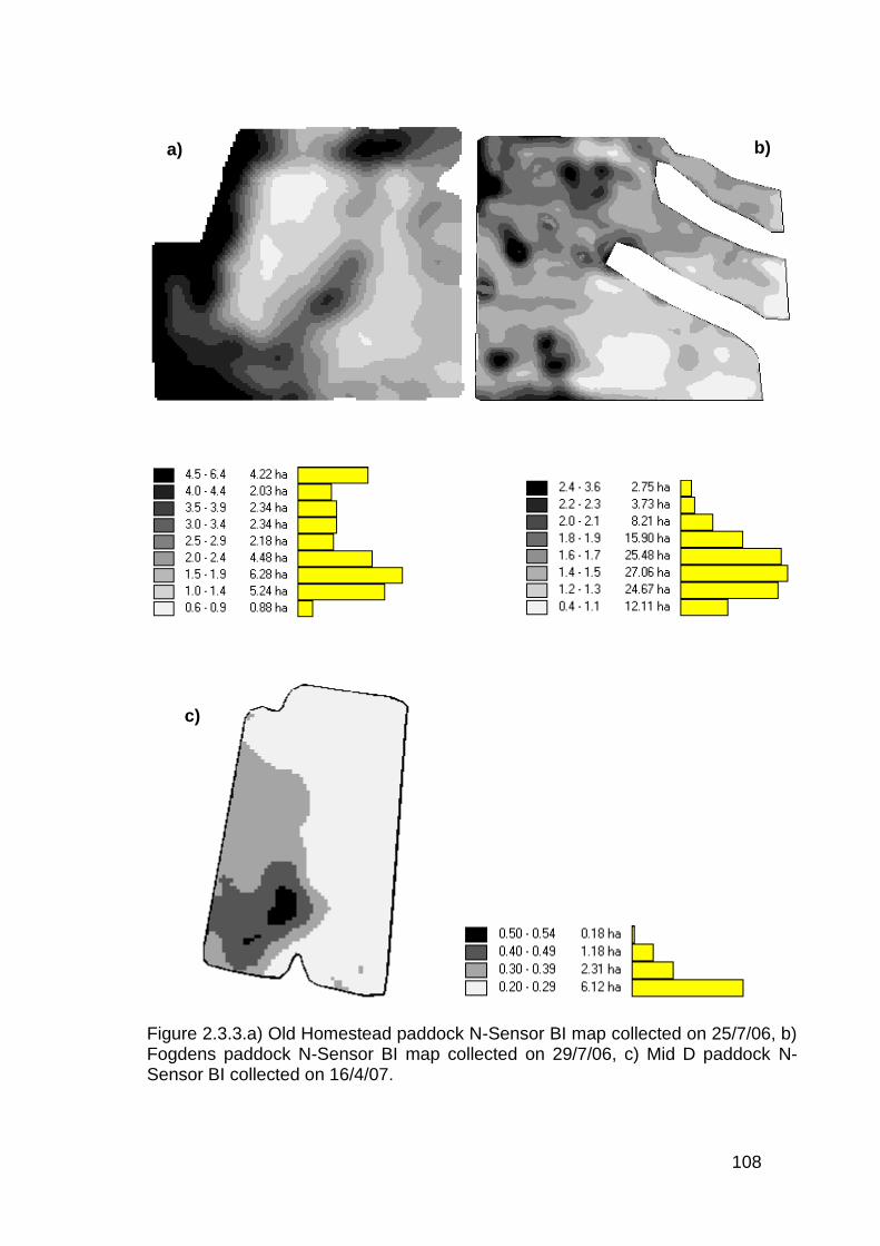
108

Figure 2.3.3.a) Old Homestead paddock N-Sensor BI map collected on 25/7/06, b) Fogdens paddock N-Sensor BI map collected on 29/7/06, c) Mid D paddock N-Sensor BI collected on 16/4/07.

a) b)

c)

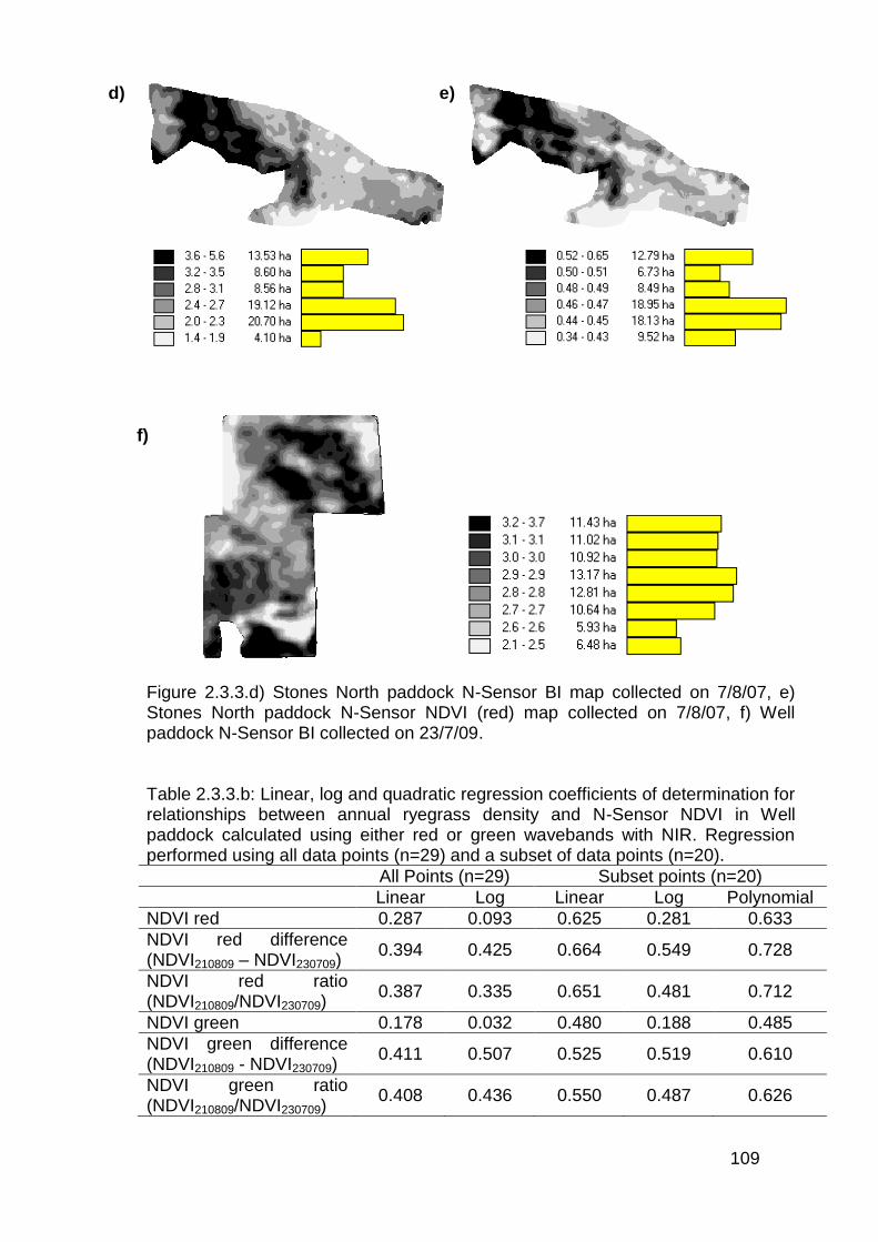
109

Figure 2.3.3.d) Stones North paddock N-Sensor BI map collected on 7/8/07, e) Stones North paddock N-Sensor NDVI (red) map collected on 7/8/07, f) Well paddock N-Sensor BI collected on 23/7/09.

Table 2.3.3.b: Linear, log and quadratic regression coefficients of determination for relationships between annual ryegrass density and N-Sensor NDVI in Well paddock calculated using either red or green wavebands with NIR. Regression performed using all data points (n=29) and a subset of data points (n=20).

All Points (n=29) Subset points (n=20)

Linear Log Linear Log Polynomial

NDVI red 0.287 0.093 0.625 0.281 0.633

NDVI red difference (NDVI210809 – NDVI230709)

0.394 0.425 0.664 0.549 0.728

NDVI red ratio (NDVI210809/NDVI230709)

0.387 0.335 0.651 0.481 0.712

NDVI green 0.178 0.032 0.480 0.188 0.485

NDVI green difference (NDVI210809 - NDVI230709)

0.411 0.507 0.525 0.519 0.610

NDVI green ratio (NDVI210809/NDVI230709)

0.408 0.436 0.550 0.487 0.626

d)

f)

e)

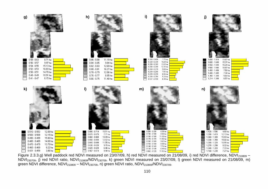
110

Figure 2.3.3.g) Well paddock red NDVI measured on 23/07/09, h) red NDVI measured on 21/08/09, i) red NDVI difference, NDVI210809 – NDVI230709, j) red NDVI ratio, NDVI210809/NDVI230709, k) green NDVI measured on 23/07/09, l) green NDVI measured on 21/08/09, m) green NDVI difference, NDVI210809 – NDVI230709, n) green NDVI ratio, NDVI210809/NDVI230709.

g)

k) l) m)

h) i) j)

n)

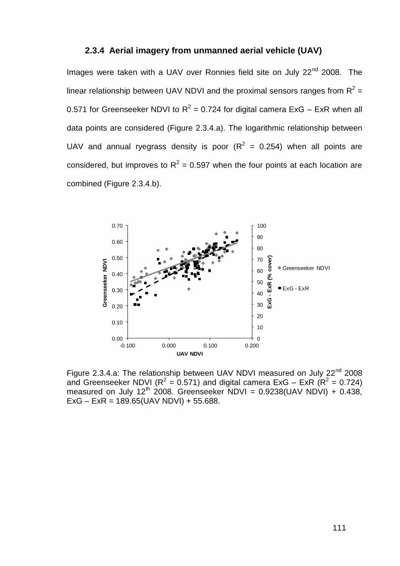
111

2.3.4 Aerial imagery from unmanned aerial vehicle (UAV)

Images were taken with a UAV over Ronnies field site on July 22nd 2008. The

linear relationship between UAV NDVI and the proximal sensors ranges from R2 =

0.571 for Greenseeker NDVI to R2 = 0.724 for digital camera ExG – ExR when all

data points are considered (Figure 2.3.4.a). The logarithmic relationship between

UAV and annual ryegrass density is poor (R2 = 0.254) when all points are

considered, but improves to R2 = 0.597 when the four points at each location are

combined (Figure 2.3.4.b).

0

10

20

30

40

50

60

70

80

90

100

0.00

0.10

0.20

0.30

0.40

0.50

0.60

0.70

-0.100 0.000 0.100 0.200

ExG

-E

xR

(%

co

ver)

Gre

en

seeker

ND

VI

UAV NDVI

Greenseeker NDVI

ExG - ExR

Figure 2.3.4.a: The relationship between UAV NDVI measured on July 22nd 2008 and Greenseeker NDVI (R2 = 0.571) and digital camera ExG – ExR (R2 = 0.724) measured on July 12th 2008. Greenseeker NDVI = 0.9238(UAV NDVI) + 0.438, ExG – ExR = 189.65(UAV NDVI) + 55.688.

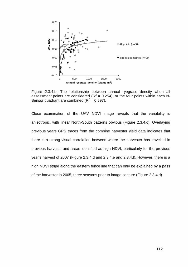
112

-0.10

-0.05

0.00

0.05

0.10

0.15

0.20

0 500 1000 1500 2000

UA

V N

DV

I

Annual ryegrass density (plants m-2)

All points (n=80)

4 points combined (n=20)

Figure 2.3.4.b: The relationship between annual ryegrass density when all assessment points are considered (R2 = 0.254), or the four points within each N-Sensor quadrant are combined (R2 = 0.597).

Close examination of the UAV NDVI image reveals that the variability is

anisotropic, with linear North-South patterns obvious (Figure 2.3.4.c). Overlaying

previous years GPS traces from the combine harvester yield data indicates that

there is a strong visual correlation between where the harvester has travelled in

previous harvests and areas identified as high NDVI, particularly for the previous

year’s harvest of 2007 (Figure 2.3.4.d and 2.3.4.e and 2.3.4.f). However, there is a

high NDVI stripe along the eastern fence line that can only be explained by a pass

of the harvester in 2005, three seasons prior to image capture (Figure 2.3.4.d).

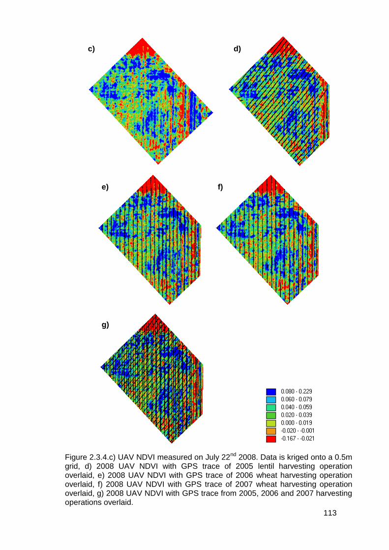
113

Figure 2.3.4.c) UAV NDVI measured on July 22nd 2008. Data is kriged onto a 0.5m grid, d) 2008 UAV NDVI with GPS trace of 2005 lentil harvesting operation overlaid, e) 2008 UAV NDVI with GPS trace of 2006 wheat harvesting operation overlaid, f) 2008 UAV NDVI with GPS trace of 2007 wheat harvesting operation overlaid, g) 2008 UAV NDVI with GPS trace from 2005, 2006 and 2007 harvesting operations overlaid.

c)

g)

f) e)

d)

114

2.4 Discussion

It is possible to map annual ryegrass density with commercially available spectral

reflectance sensors based on the principal that areas of higher density produce a

greater vegetative index response. However, there are a range of crop and weed

factors that will influence the accuracy of the map generated. No wavelengths

were identified in the annual ryegrass spectral signature in this study that

discriminate annual ryegrass patches from other species (Figure 2.3.1.1.a and

2.3.1.1.d). Therefore, the vegetative indices assessed were responsive to changes

in total plant growth, rather than those of the target weed only.

The regressions between annual ryegrass density and digital camera ExG – ExR

outputs were consistently as good as, if not better than, those of the spectral

sensors (Figure 2.3.1.4.a and 2.3.1.4.c). In particular, the camera positioned 27˚

above ground level at 1.5 m height was better than the camera positioned directly

above the target (Table 2.3.1.2.a, Figure 2.3.1.2.a & b). The amount of cloud cover

and the intensity and direction of sunlight appears to affect the misclassification of

stubble as plant cover in this study (Table 2.3.1.2.b, 2.3.1.2.c, 2.3.1.2.d and

2.3.1.2.e). However, the potential for vision-based systems for weed detection in

these cropping systems is promising and methods for excluding the crop row from

classification as proposed by Hague et al. (2006) warrant further investigation.

Surprisingly, in the stationary point measurement experiments, calculating the

mean for the sensor and annual ryegrass data collected from the four N-Sensor

quadrants improved the regressions between sensor data and annual ryegrass

density compared with regression of all data points (Table 2.3.1.3.a, Figure

2.3.1.3.a and Figure 2.3.1.3.b). This was due to a mismatch in the resolution of

115

annual ryegrass density assessment and the field of view of the sensors. The

original intention was to attempt to identify the large scale patch variability in

annual ryegrass density; however, there was also significant small scale variability

in annual ryegrass density that occurred in the order of less than a metre, i.e. the

spatial pattern of annual ryegrass distribution did not exhibit scale invariance, and

it is not apparent why plant populations would exhibit scale invariance (Cousens et

al. 2004). A number of processes will lead to either more or less aggregation and

these occur at a number of distinct characteristic scales. This scale variance

meant that there was significant variability in annual ryegrass density within the

area assessed by the sensors and a single assessment of annual ryegrass density

with a 0.1m2 quadrat did not adequately represent the density the sensors were

viewing. Taking more counts across the sensors field of view is likely to have

helped overcome this problem. Combining the four data points at each (N-Sensor)

location has removed some of the short scale variability and the measurements

are more closely aligned with the variability at the patch scale.

Changes in annual ryegrass density were easier to detect when the ryegrass was

at mid tillering (GS23-25) compared with earlier growth stages, particularly in

Ronnies paddock (Figure 2.3.1.1.b, 2.3.1.1.e, 2.3.1.4.a, 2.3.1.4.d and Table

2.3.1.2.a and 2.3.1.3.a). This is despite the fact that in Ronnies paddock there

was a negative correlation between annual ryegrass density and lentil growth

established at the 4th timing on July 12th (Figure 2.3.1.5.b and Table 2.3.1.5.a),

which means that the sensor response to increased annual ryegrass growth would

be offset by a reduction in crop growth. It is likely that this relationship was a result

of the competitive effect of annual ryegrass against lentils restricting lentil growth.

However, the same effect was not observed in Stones South paddock in peas.

116

Annual ryegrass at early growth stages (GS11-22) has a small leaf area; therefore

its contribution to spectral reflectance at early growth stages even when at high

densities is low. The relative growth rate of annual ryegrass was greater than that

of both lentil and pea over the early growth stages (Table 2.3.1.5.a and 2.3.1.5.c).

Over the same period the variability in crop dry matter is low (Figure 2.3.1.5.a and

2.3.1.5.d). This means annual ryegrass is having a greater effect on sensor

response with subsequent sensor timings. In Ronnies paddock, the improvement

in annual ryegrass detection with later timings is not observed at the 4th timing on

July 12th, and this corresponds with the timing when annual ryegrass is having a

negative effect on lentil growth.

The slope of the curve was found to be important in determining the best fit

models in some cases. A lower slope implies that any error in a sensor reading will

be amplified when predicting annual ryegrass density, whereas with a steeper

slope the same error in sensor reading will lead to a smaller error in prediction of

annual ryegrass density. It was found that indices calculated using NIR (780nm)

and either red (670nm), green (550nm) or blue (450nm) reflectance could produce

similar R2 values, but the slope of the curves using red reflectance was always

steeper, indicating these indices are more responsive to changes in annual

ryegrass density, particularly at the lower densities (Figure 2.3.1.1.b, c, e & f).

Sensor position also affected curve slope and coefficient of determination. It was

shown that the camera mounted at an angle had better R2 and steeper slope than

when mounted directly above the field of view (Table 2.3.1.2.a, Figure 2.3.1.2.a, b,

c & d). Similar trends were observed when comparing N-Sensor NDVI,

Greenseeker and Crop Circle, where the N-Sensor generally had a better fit and

steeper slope (Figure 2.3.1.4.a, b, c, d, e, f), particularly at earlier growth stages.

117

In both cases, the improvement can be explained by the difference in view of the

target, given annual ryegrass has an upright growth habit. From directly above,

the reflective green leaf area visible to the sensor is only a small percentage of the

total green leaf area. This is the view that the Greenseeker, Crop Circle and

digital camera see when positioned directly above the target. This is contrasted by

the N-Sensor and digital camera mounted at 27° above horizontal. These sensors

view more of the annual ryegrass green leaf area and are therefore more

responsive to change in annual ryegrass density, particularly at the pre tillering

stages.

The costs associated with weed mapping are an important consideration in the

overall economics of site specific weed management (Goudy et al. 2001; Lutman

& Miller 2007). In a practical sense in lentils and peas, the optimal time for

mapping annual ryegrass will be at or shortly before the grasses are sprayed with

a selective herbicide. To save on mapping costs the mapping and spraying

operations could be carried out in the same pass.

The herbicide diflufenican was observed to slow lentil growth after its application

and no lentil growth was measured between July 1st and 12th (Table 2.3.1.5.a).

This presents an opportunity where plant growth measured between July 1st and

12th, using a sensor, might be attributed to annual ryegrass growth alone. This

theory was tested where either the N-Sensor NDVI (red) difference (N-Sensor

NDVI120708 - N-Sensor NDVI010708) or N-Sensor NDVI (red) ratio (N-Sensor

NDVI120708/N-Sensor NDVI010708) were regressed with annual ryegrass density.

There was a decline in the strength of the regression from doing this (Figure

2.3.1.5.c). While there was an overall stagnation in lentil growth across the field,

118

there was variability in growth between sites with some sites continuing to grow

and others showing a biomass decline (Figure 2.3.1.5.a). This increased

variability in crop growth may be the cause of the decline in regression strength

from calculating the change between sensor dates.

The application of clethodim and quizalofop on July 15th provided good control of

annual ryegrass at this site and once the annual ryegrass had senesced its

influence on sensor response was removed. It was therefore expected that the

change in sensor measurement from pre to post clethodim application would show

areas with low annual ryegrass density as having the greatest positive change

while areas with high annual ryegrass densities that were controlled having the

lowest change in sensor measurement. This is because the lentils continue to

grow contributing to a positive change in sensor response, but this is offset where

high densities of annual ryegrass have been removed. This hypothesis was tested

where either the N-Sensor NDVI (red) difference (N-Sensor NDVI210808 - N-Sensor

NDVI120708) or N-Sensor NDVI (red) ratio (N-Sensor NDVI210808/N-Sensor

NDVI120708) were regressed with annual ryegrass density. The strength of the

regression was improved from R2 = 0.63 for sensing on both July 1st and 12th to

0.76 for the change between sensing pre and post clethodim application (Figure

2.3.1.5.c).

This was also tested at the paddock scale in the Well paddock and the change

between sensing dates from pre and post clethodim application was again found

to improve the correlation with annual ryegrass density (Table 2.3.3.b and Figure

2.3.3.g-n). This paddock consists of dunes and swales, so in addition to variability

in annual ryegrass density it also had variability in brome grass density and

119

significant variability in crop growth with poorer crop growth on lighter sands and

vigorous crop growth in some loamy flats. The herbicide application also

controlled brome grass, so the change map does not help to discriminate brome

patches from annual ryegrass, however it does help to remove some of the

variability induced by variable crop growth. The most obvious example of this is in

the south western corner of the Well paddock where there is a low weed burden

but vigorous crop growth. When the pre clethodim map from July 23rd (Figure

2.3.3.g and 2.3.3.k) is considered in isolation this area would be likely

misclassified as weedy as it has a high N-Sensor NDVI value. However, when

considered in conjunction with the post clethodim map from August 21st and a

change map is generated it is apparent that this is an area of vigorous crop growth

and not high weed burden. In addition, there are regions within this paddock that

have a high weed burden, but due to poor crop growth on lighter sands the NDVI

value on July 23rd is low such that it is likely misclassified as weed free. Again,

consideration of the change map helps to identify these areas as weedy as they

don’t change significantly from pre clethodim application to post clethodim

application. Mapping the paddock twice will increase the cost of generating an

annual ryegrass map. The post clethodim mapping timing could possibly be

combined with an early fungicide application in lentils that are targeted at the

timing just prior to canopy closure to help minimise the mapping cost.

Annual ryegrass is detectable in wheat, at high densities. Annual ryegrass density

of 318 plants m-2 resulted in significantly higher measurement of Greenseeker

NDVI and the digital camera ExG - ExR compared with the background density of

7 plants m-2 (Table 2.3.2.a). The effect of high density annual ryegrass was

significant at all sensing dates for both the Greenseeker NDVI and digital camera

120

algorithm, whereas the effect of nitrogen treatment was not significant until the last

sensing date when the crop was at GS33, and only with the Greenseeker. This is

because many plant stresses influence canopy spectral reflectance (Goel et al.

2003; Fitzgerald et al. 2010). However, in this circumstance the effect of crop

nitrogen nutrition was not evident until later in the crop’s growth when the nitrogen

demand of the crop is much higher. It is expected that in well managed crops this

would typically be the case, where crop growth is relatively uniform at early growth

stages while the crop nutrient demand is low and the plants are growing from seed

reserves.

The digital camera ExG – ExR algorithm produces an output of percent cover,

which is related to the percentage of green pixels in an image, but not the intensity

of green, i.e. the pixel is green or it isn’t. NDVI values are responsive to changes in

green leaf area, but also to chlorophyll activity through the measurement of red

light reflectance. This will help to explain the difference between the Greenseeker

NDVI and digital camera ExG – ExR response to N treatment at GS33, where the

Greenseeker response was significant for both ryegrass density and N treatment,

suggesting a combined response to the effect of green leaf area and green

intensity generated by the N treatments, whereas the digital camera ExG – ExR

was only responsive to ryegrass treatment indicating a response to changes in

green leaf area only.

The variability in density of non-target weed species significantly reduced the

correlations between sensor measurement and annual ryegrass density, as the

sensors are responsive to green plant matter, regardless of species. This was

evident at numerous sites including Ronnies, Stones South, Fogdens and the Well

121

paddock where snail medic, wild oat, wild oat and brome grass were present,

respectively. Accounting for non target weed presence helped to explain more of

the variability in sensor readings. Including the weed dry matter in the analysis

improved the correlations in Ronnies (Figure 2.3.1.6.a), but reduced the

correlation in Stones South (Figure 2.3.1.6.b). Simply excluding the points where

those weeds were present at high density improved the correlations at all sites

(Figure 2.3.1.6.a and 2.3.1.6.b and Table 2.3.3.a). The interpretation of sensor

maps may be confounded by non target species in this study, but they may still be

of value to the grower. The high densities of these weeds observed at these sites

will have significant negative impacts on yield and financial return from these

areas and are likely to warrant control. Where non target species confound a map,

it might, at best, be possible to identify a weed control strategy that will target both

weed species. This is likely to be more applicable where annual ryegrass is found

in combination with brome grass or wild oat, where selective herbicides may be

available that control both species. At worst, the misclassification of a non target

species as annual ryegrass will result in the over application of the annual

ryegrass control measure, which may have no control of the non target weed

species. This is likely to be the case with annual ryegrass and snail medic, unless

the control measure is non-selective and controls all species.

Annual ryegrass distribution is influenced by the operation of the harvester, where

the seed is concentrated in rows behind the harvester (Blanco-Moreno et al.

2004), causing anisotropic distribution patterns (Figure 2.4.c, d, e, f and g). This

has implications for the spatial resolution of mapping and proximal sensor

placement for mapping. To ensure no high density patches are missed, proximal

sensors should be oriented so that they are over the previous year’s harvester

122

row, otherwise the size and density of annual ryegrass patches are likely to be

significantly underestimated. The sensor spacing will therefore be related to the

width of the harvester, which typically ranges from 9.1 m to 13.7 m. This would

require a strategic plan at harvest time, to ensure that a systematic pattern is

followed for ease of mapping. A controlled traffic system would aid this, or at least

using the same A-B navigation lines for harvest each year.

123

3 Patch Stability in Lolium rigidum Populations

3.1 Introduction

The stability of patches is important, as it impacts on how long a map will suitably

describe the spatial distribution of a given weed population and therefore the

frequency of mapping required to maintain an accurate weed map. The cost of

mapping is significant for the overall profitability of patch spraying and therefore

mapping frequency will have a significant impact on the overall profitability of patch

spraying (Goudy et al. 2001; Lutman & Miller 2007). Weed density data collected

at specific locations over several years is commonly used to assess patch stability.

A review of the literature by Lutman and Miller (2007) shows that these

correlations are much lower than 1.0 (R2), with the studies reported showing

correlations ranging from 0.15 to 0.46. Rew et al. (2001) report correlation

coefficients from three consecutive years 1997-1999 with a range of 0.369 to

0.784, the highest correlation being obtained between years 1997 and 1999.

Flaws in using correlation techniques for year to year comparisons can partly

explain these low correlations. For example, if weeds are more abundant in one

year than another then the patch appears to expand and, although the patch has

not moved, the correlations will be poor (Lutman & Miller 2007). Location (GPS)

errors may also contribute to reducing correlations, especially when weed density

varies greatly over distances smaller than the GPS accuracy.

Several studies have found that weed patch centres tend to be stable over time;

however, significant fluctuations in patch boundary location and weed densities

124

between seasons are more common (Cardina et al. 1997; Mortensen & Dieleman

1997; Dieleman & Mortensen 1999; Rew & Cousens 2001).

Variability in total seed production is expected to cause patches to expand in years

after high production and contract in years after low production (Dieleman &

Mortensen 1999). Indeed, Gerhards et al. (1997) found that years with high mean

seedling density corresponded with the largest patch sizes. The size of the seed

bank is an indication of potential weed emergence (Nordmeyer 2005); however,

studies have shown for some species that there is often considerable lack of

correlation between the seed bank and resulting weed emergence (Grundy 1997).

Blanco-Moreno et al. (2004) suggest that in the case of annual ryegrass the

existing seed bank is less important due to the short life of seeds in the soil and

more consideration should be given to the seed rain from the previous season.

Seed rain, seed bank density and persistence of seed in the seed bank are

important features of a weed species that influence the stability of weed patches

between seasons. The aim of this study is to assess the stability of annual

ryegrass populations between seasons across crop rotations including wheat,

barley, oaten and wheaten hay, canola, peas and lentils.

3.2 Materials and Methods

Annual ryegrass density was assessed at point locations in four farmers’ paddocks

in three cropping seasons. Data collection and paddock details are described

below (Table 3.2.a). At each assessment annual ryegrass density was assessed

using one of the three methods described below:

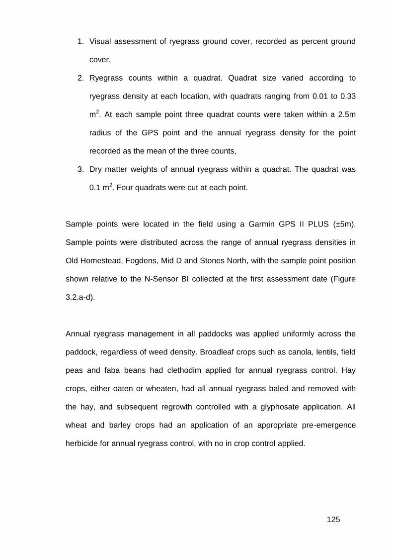
125

1. Visual assessment of ryegrass ground cover, recorded as percent ground

cover,

2. Ryegrass counts within a quadrat. Quadrat size varied according to

ryegrass density at each location, with quadrats ranging from 0.01 to 0.33

m2. At each sample point three quadrat counts were taken within a 2.5m

radius of the GPS point and the annual ryegrass density for the point

recorded as the mean of the three counts,

3. Dry matter weights of annual ryegrass within a quadrat. The quadrat was

0.1 m2. Four quadrats were cut at each point.

Sample points were located in the field using a Garmin GPS II PLUS (±5m).

Sample points were distributed across the range of annual ryegrass densities in

Old Homestead, Fogdens, Mid D and Stones North, with the sample point position

shown relative to the N-Sensor BI collected at the first assessment date (Figure

3.2.a-d).

Annual ryegrass management in all paddocks was applied uniformly across the

paddock, regardless of weed density. Broadleaf crops such as canola, lentils, field

peas and faba beans had clethodim applied for annual ryegrass control. Hay

crops, either oaten or wheaten, had all annual ryegrass baled and removed with

the hay, and subsequent regrowth controlled with a glyphosate application. All

wheat and barley crops had an application of an appropriate pre-emergence

herbicide for annual ryegrass control, with no in crop control applied.

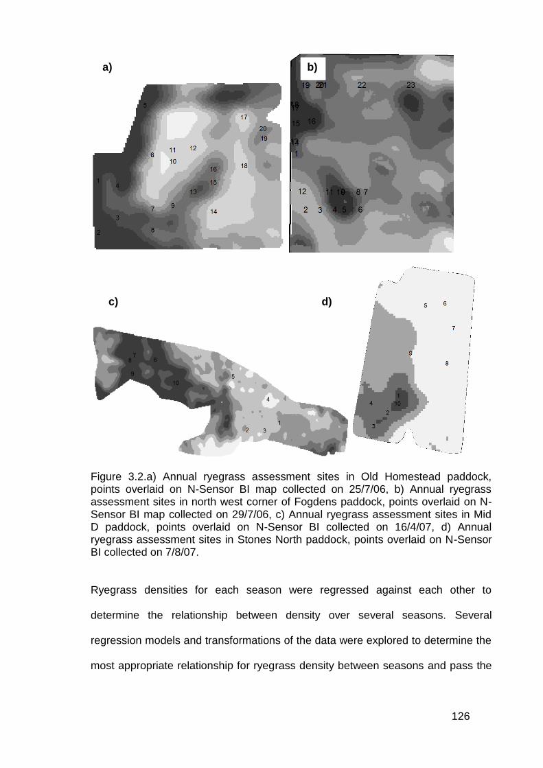
126

Figure 3.2.a) Annual ryegrass assessment sites in Old Homestead paddock, points overlaid on N-Sensor BI map collected on 25/7/06, b) Annual ryegrass assessment sites in north west corner of Fogdens paddock, points overlaid on N-Sensor BI map collected on 29/7/06, c) Annual ryegrass assessment sites in Mid D paddock, points overlaid on N-Sensor BI collected on 16/4/07, d) Annual ryegrass assessment sites in Stones North paddock, points overlaid on N-Sensor BI collected on 7/8/07.

Ryegrass densities for each season were regressed against each other to

determine the relationship between density over several seasons. Several

regression models and transformations of the data were explored to determine the

most appropriate relationship for ryegrass density between seasons and pass the

a) b)

d) c)

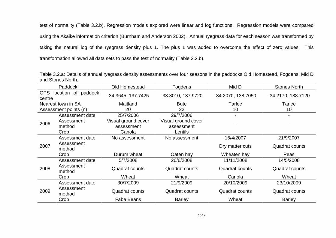
127

test of normality (Table 3.2.b). Regression models explored were linear and log functions. Regression models were compared

using the Akaike information criterion (Burnham and Anderson 2002). Annual ryegrass data for each season was transformed by

taking the natural log of the ryegrass density plus 1. The plus 1 was added to overcome the effect of zero values. This

transformation allowed all data sets to pass the test of normality (Table 3.2.b).

Table 3.2.a: Details of annual ryegrass density assessments over four seasons in the paddocks Old Homestead, Fogdens, Mid D and Stones North.

Paddock Old Homestead Fogdens Mid D Stones North

GPS location of paddock centre

-34.3645, 137.7425 -33.8010, 137.9720 -34.2070, 138.7050 -34.2170, 138.7120

Nearest town in SA Maitland Bute Tarlee Tarlee Assessment points (n) 20 22 10 10

2006

Assessment date 25/7/2006 29/7/2006 - - Assessment method

Visual ground cover assessment

Visual ground cover assessment

- -

Crop Canola Lentils

2007

Assessment date No assessment No assessment 16/4/2007 21/9/2007 Assessment method

Dry matter cuts Quadrat counts

Crop Durum wheat Oaten hay Wheaten hay Peas

2008

Assessment date 5/7/2008 26/6/2008 11/11/2008 14/5/2008 Assessment method

Quadrat counts Quadrat counts Quadrat counts Quadrat counts

Crop Wheat Wheat Canola Wheat

2009

Assessment date 30/7/2009 21/9/2009 20/10/2009 23/10/2009 Assessment method

Quadrat counts Quadrat counts Quadrat counts Quadrat counts

Crop Faba Beans Barley Wheat Barley

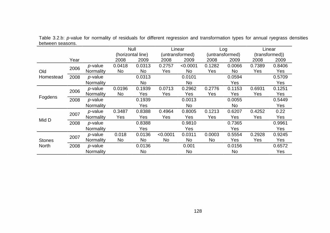
128

Table 3.2.b: p-value for normality of residuals for different regression and transformation types for annual ryegrass densities between seasons.

Null (horizontal line)

Linear (untransformed)

Log (untransformed)

Linear (transformed))

Year 2008 2009 2008 2009 2008 2009 2008 2009

Old Homestead

2006 p-value 0.0418 0.0313 0.2757 <0.0001 0.1282 0.0066 0.7389 0.8406

Normality No No Yes No Yes No Yes Yes

2008 p-value 0.0313 0.0101 0.0594 0.5709

Normality No No Yes Yes

Fogdens

2006 p-value 0.0196 0.1939 0.0713 0.2962 0.2776 0.1153 0.6931 0.1251

Normality No Yes Yes Yes Yes Yes Yes Yes

2008 p-value 0.1939 0.0013 0.0055 0.5449

Normality Yes No No Yes

Mid D

2007 p-value 0.3487 0.8388 0.4964 0.8005 0.1213 0.6207 0.4252 0.22

Normality Yes Yes Yes Yes Yes Yes Yes Yes

2008 p-value 0.8388 0.9810 0.7365 0.9961

Normality Yes Yes Yes Yes

Stones North

2007 p-value 0.018 0.0136 <0.0001 0.0311 0.0003 0.5554 0.2928 0.9245

Normality No No No No No Yes Yes Yes

2008 p-value 0.0136 0.001 0.0156 0.6572

Normality No No No Yes

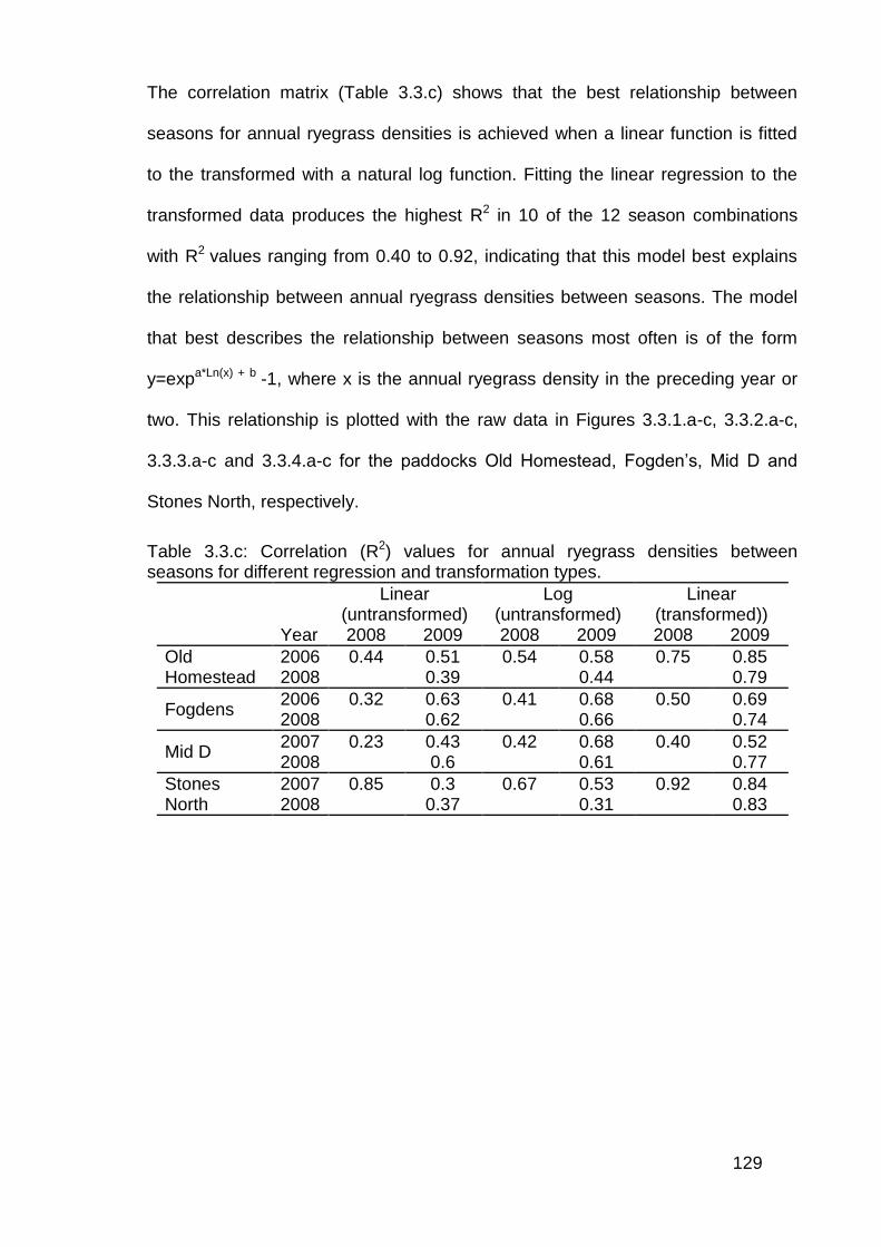
129

The correlation matrix (Table 3.3.c) shows that the best relationship between

seasons for annual ryegrass densities is achieved when a linear function is fitted

to the transformed with a natural log function. Fitting the linear regression to the

transformed data produces the highest R2 in 10 of the 12 season combinations

with R2 values ranging from 0.40 to 0.92, indicating that this model best explains

the relationship between annual ryegrass densities between seasons. The model

that best describes the relationship between seasons most often is of the form

y=expa*Ln(x) + b -1, where x is the annual ryegrass density in the preceding year or

two. This relationship is plotted with the raw data in Figures 3.3.1.a-c, 3.3.2.a-c,

3.3.3.a-c and 3.3.4.a-c for the paddocks Old Homestead, Fogden’s, Mid D and

Stones North, respectively.

Table 3.3.c: Correlation (R2) values for annual ryegrass densities between seasons for different regression and transformation types.

Linear (untransformed)

Log (untransformed)

Linear (transformed))

Year 2008 2009 2008 2009 2008 2009

Old Homestead

2006 0.44 0.51 0.54 0.58 0.75 0.85 2008 0.39 0.44 0.79

Fogdens 2006 0.32 0.63 0.41 0.68 0.50 0.69 2008 0.62 0.66 0.74

Mid D 2007 0.23 0.43 0.42 0.68 0.40 0.52 2008 0.6 0.61 0.77

Stones North

2007 0.85 0.3 0.67 0.53 0.92 0.84 2008 0.37 0.31 0.83

130

3.3 Results

The combined exponential and natural log function shows that, despite a high level

of scatter between annual ryegrass densities between seasons, there is a strong

positive correlation between ryegrass densities between seasons. In general,

locations with relatively lower ryegrass density in one year will have relatively

lower ryegrass density in subsequent years and locations with relatively higher

ryegrass densities in one year will have relatively higher ryegrass densities in

subsequent years. The shape of the curve indicates that annual ryegrass will

increase at a faster rate when at low densities than when at high densities, with

the curve generally having a steeper slope as the curve approaches zero.

There is significantly more scatter around the line of best fit as ryegrass densities

increase. However, there are few examples where the population goes from being

relatively high in the first year to relatively low in subsequent years. For the four

paddocks there were 93 observations that were above the paddock median in the

initial year of comparison, only 8 (8.6% of total) of these positions fell below the

paddock median in the subsequent year of comparison (Table 3.3.a). Five of the

eight position by season comparisons that fell below the median in a subsequent

year were in the Mid D paddock and three in Fogdens paddock. Of these eight

position by season comparisons that changed relative to the median, four are

explained by two positions that were greater than the median in 2006 or 2007, and

then less than the median in both 2008 and 2009 (Table 3.3.b).

There were 16 (17.2% of total) positions by season comparisons that increased to

be greater than the paddock median in a subsequent year after being below the

paddock median in the first year of comparison. Ten of these changes can be

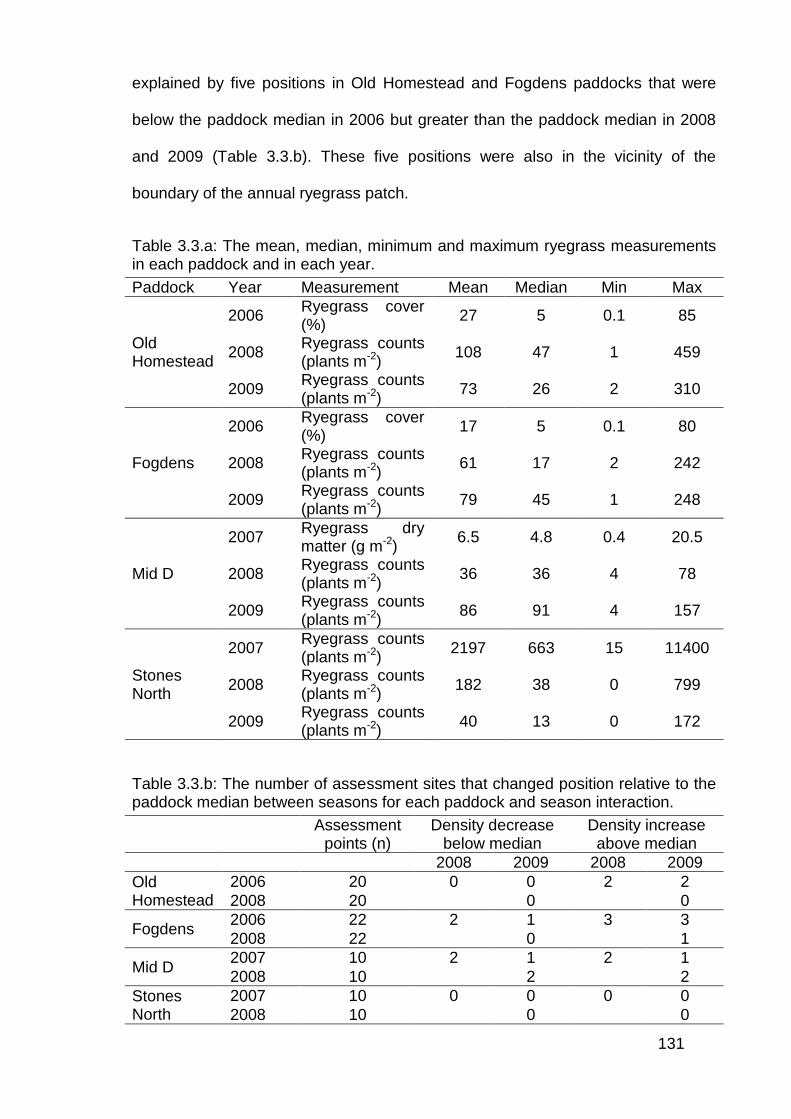
131

explained by five positions in Old Homestead and Fogdens paddocks that were

below the paddock median in 2006 but greater than the paddock median in 2008

and 2009 (Table 3.3.b). These five positions were also in the vicinity of the

boundary of the annual ryegrass patch.

Table 3.3.a: The mean, median, minimum and maximum ryegrass measurements in each paddock and in each year.

Paddock Year Measurement Mean Median Min Max

Old Homestead

2006 Ryegrass cover (%)

27 5 0.1 85

2008 Ryegrass counts (plants m-2)

108 47 1 459

2009 Ryegrass counts (plants m-2)

73 26 2 310

Fogdens

2006 Ryegrass cover (%)

17 5 0.1 80

2008 Ryegrass counts (plants m-2)

61 17 2 242

2009 Ryegrass counts (plants m-2)

79 45 1 248

Mid D

2007 Ryegrass dry matter (g m-2)

6.5 4.8 0.4 20.5

2008 Ryegrass counts (plants m-2)

36 36 4 78

2009 Ryegrass counts (plants m-2)

86 91 4 157

Stones North

2007 Ryegrass counts (plants m-2)

2197 663 15 11400

2008 Ryegrass counts (plants m-2)

182 38 0 799

2009 Ryegrass counts (plants m-2)

40 13 0 172

Table 3.3.b: The number of assessment sites that changed position relative to the paddock median between seasons for each paddock and season interaction.

Assessment points (n)

Density decrease below median

Density increase above median

2008 2009 2008 2009

Old Homestead

2006 20 0 0 2 2

2008 20 0 0

Fogdens 2006 22 2 1 3 3

2008 22 0 1

Mid D 2007 10 2 1 2 1

2008 10 2 2

Stones North

2007 10 0 0 0 0

2008 10 0 0

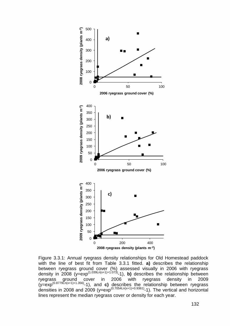
132

0

100

200

300

400

500

0 50 100

2008 r

yeg

rass d

en

sit

y (

pla

nts

m-2

)

2006 ryegrass ground cover (%)

a)

0

50

100

150

200

250

300

350

400

0 50 100

2009 r

yeg

rass d

en

sit

y (

pla

nts

m-2

)

2006 ryegrass ground cover (%)

b)

0

50

100

150

200

250

300

350

400

0 200 400

2009 r

yeg

rass d

en

sit

y (

pla

nts

m-2

)

2008 ryegrass density (plants m -2)

c)

Figure 3.3.1: Annual ryegrass density relationships for Old Homestead paddock with the line of best fit from Table 3.3.1 fitted. a) describes the relationship between ryegrass ground cover (%) assessed visually in 2006 with ryegrass density in 2008 (y=exp(1.039Ln(x+1)+1.073)-1), b) describes the relationship between ryegrass ground cover in 2006 with ryegrass density in 2009 (y=exp(0.8779Ln(x+1)+1.356)-1), and c) describes the relationship between ryegrass densities in 2008 and 2009 (y=exp(0.7054Ln(x+1)+0.9361)-1). The vertical and horizontal lines represent the median ryegrass cover or density for each year.

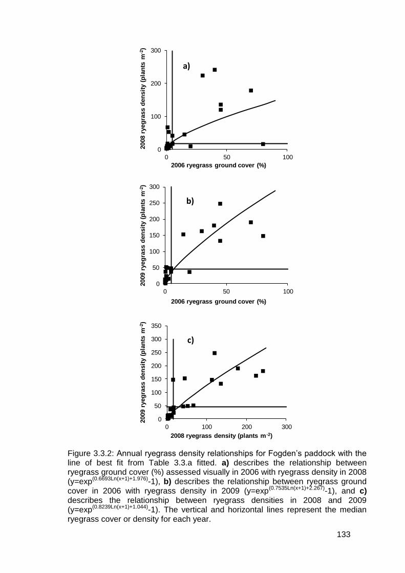
133

0

100

200

300

0 50 100

2008 r

yeg

rass d

en

sit

y (

pla

nts

m-2

)

2006 ryegrass ground cover (%)

a)

0

50

100

150

200

250

300

0 50 100

2009 r

yeg

rass d

en

sit

y (

pla

nts

m-2

)

2006 ryegrass ground cover (%)

b)

0

50

100

150

200

250

300

350

0 100 200 300

2009 r

yeg

rass d

en

sit

y (

pla

nts

m-2

)

2008 ryegrass density (plants m -2)

c)

Figure 3.3.2: Annual ryegrass density relationships for Fogden’s paddock with the line of best fit from Table 3.3.a fitted. a) describes the relationship between ryegrass ground cover (%) assessed visually in 2006 with ryegrass density in 2008 (y=exp(0.6693Ln(x+1)+1.976)-1), b) describes the relationship between ryegrass ground cover in 2006 with ryegrass density in 2009 (y=exp(0.7535Ln(x+1)+2.267)-1), and c) describes the relationship between ryegrass densities in 2008 and 2009 (y=exp(0.8239Ln(x+1)+1.044)-1). The vertical and horizontal lines represent the median ryegrass cover or density for each year.

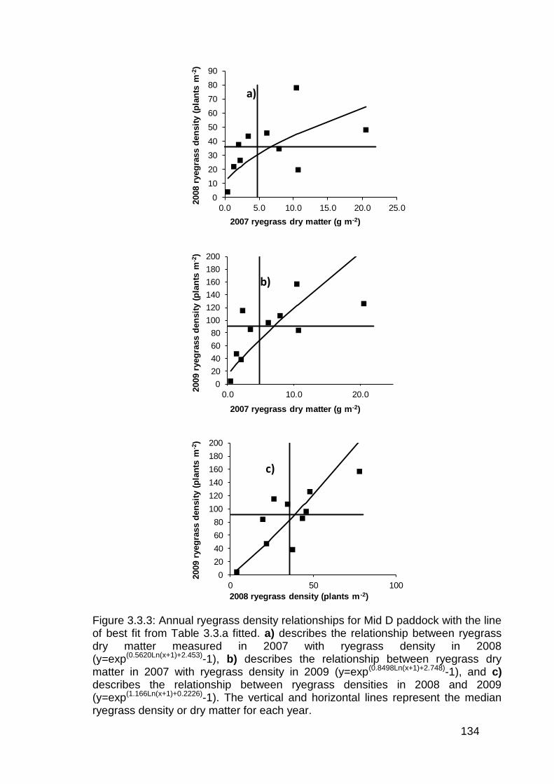
134

0

10

20

30

40

50

60

70

80

90

0.0 5.0 10.0 15.0 20.0 25.0

2008 r

yeg

rass d

en

sit

y (

pla

nts

m-2

)

2007 ryegrass dry matter (g m-2)

a)

0

20

40

60

80

100

120

140

160

180

200

0.0 10.0 20.0

2009 r

yeg

rass d

en

sit

y (

pla

nts

m-2

)

2007 ryegrass dry matter (g m-2)

b)

0

20

40

60

80

100

120

140

160

180

200

0 50 100

2009 r

yeg

rass d

en

sit

y (

pla

nts

m-2

)

2008 ryegrass density (plants m -2)

c)

Figure 3.3.3: Annual ryegrass density relationships for Mid D paddock with the line of best fit from Table 3.3.a fitted. a) describes the relationship between ryegrass dry matter measured in 2007 with ryegrass density in 2008 (y=exp(0.5620Ln(x+1)+2.453)-1), b) describes the relationship between ryegrass dry matter in 2007 with ryegrass density in 2009 (y=exp(0.8498Ln(x+1)+2.748)-1), and c) describes the relationship between ryegrass densities in 2008 and 2009 (y=exp(1.166Ln(x+1)+0.2226)-1). The vertical and horizontal lines represent the median ryegrass density or dry matter for each year.

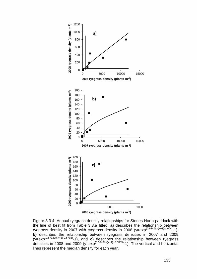
135

0

200

400

600

800

1000

1200

0 5000 10000 15000

2008 r

yeg

rass d

en

sit

y (

pla

nts

m-2

)

2007 ryegrass density (plants m -2)

a)

0

20

40

60

80

100

120

140

160

180

200

0 5000 10000 15000

2009 r

yeg

rass d

en

sit

y (

pla

nts

m-2

)

2007 ryegrass density (plants m -2)

b)

0

20

40

60

80

100

120

140

160

180

200

0 500 1000

2009 r

yeg

rass d

en

sit

y (

pla

nts

m-2

)

2008 ryegrass density (plants m -2)

c)

Figure 3.3.4: Annual ryegrass density relationships for Stones North paddock with the line of best fit from Table 3.3.a fitted. a) describes the relationship between ryegrass density in 2007 with ryegrass density in 2008 (y=exp(0.9346Ln(x+1)-1.904)-1), b) describes the relationship between ryegrass densities in 2007 and 2009 (y=exp(0.5792Ln(x+1)-0.5792)-1), and c) describes the relationship between ryegrass densities in 2008 and 2009 (y=exp(0.5943Ln(x+1)+0.6809)-1). The vertical and horizontal lines represent the median density for each year.

136

3.4 Discussion

The consistency in the shape of the curves describing the relationship between

ryegrass densities between seasons indicates that a relatively robust relationship

exists. That is, where ryegrass densities are relatively high in one season it is

likely that they will be relatively high in subsequent seasons. Conversely, where

ryegrass densities are relatively low in one season it is likely that they will be

relatively low in subsequent seasons. Data from Old Homestead and Fogdens

indicates that these relationships can be valid for up to three years with annual

ryegrass cover data from 2006 explaining 85% and 69% of the variability observed

in the 2009 annual ryegrass density data, respectively. Thus, this indicates that an

accurately produced map of annual ryegrass may describe the location of annual

ryegrass patches for several years.

Correlations of 0.40 to 0.92 for the exponential natural log function (Table 3.2.c)

are significantly higher than those reported by Lutman and Miller (2007) and Rew

et al. (2001). The fact that annual ryegrass seed is naturally dispersed over short

distances only, in the order of one to two metres (Blanco-Moreno et al. 2004), may

increase patch stability of annual ryegrass compared to other species that

disperse seed over much bigger distances. Colbach et al. (2000) found that the

level of patch persistence is most likely the result of dispersal rate, dispersal

distance and the ability of a weed to colonise and that, in general, persistence is

greater for perennial weed species with low dispersal rates than for annual weed

species with high dispersal rates. These factors have also been found to be

important in affecting the level of patchiness exhibited by a weed species

(Dieleman & Mortensen 1999; Paice et al. 1998), and density has also been found

to be inversely related to patchiness (Wiles & Brodahl 2004). The pattern of weed

137

seed dispersal and patch spread is also important in determining the usefulness of

historical weed maps for use in future seasons.

Potentially, weed populations that spread with a closed advancing front (‘phalanx

spread’) can be mapped at an earlier date and potentially be used for several

seasons as the patch spread is predictable. However, populations where a small

proportion of seeds may be moved large but unpredictable distances to form new

colonies (‘guerrilla spread’), may not be suited to use of a map of weed

infestations over several years, without a well structured monitoring program to

detect new patches (Woolcock & Cousens 2000; Wallinga et al. 2002; Barroso et

al. 2006). Natural dispersal of annual ryegrass uses a phalanx spread strategy,

while spread by harvesters is less predictable and more of a guerrilla spread

strategy.

The data shows that a position can change from having relatively high ryegrass

density to relatively low ryegrass density or vice versa in some cases (Table

3.3.b). The paddock median for each year has been used as a threshold value to

highlight this occurrence (Table 3.3.a). In general, a position changing from a

relatively high density to a relatively low density will be of little concern to growers,

but will lead to an over application of herbicide or other control measure. This will

reduce the benefit that can be achieved from SSWM through saved inputs. A

position changing from a relatively low density to a relatively high density will;

however, be of greater concern to growers. This is because they are generally

concerned more about missing weeds and having escapes that will proliferate for

following years, than over application of inputs. Five positions in Old Homestead

and Fogdens paddocks changed from relatively low to relatively high from season

138

2006 to 2008 and were still high relative to the paddock median in 2009 (Table

3.3.b). All five of these positions were in the vicinity of a patch boundary. Areas

within the vicinity of the patch boundary may be subject to more variability

between seasons for two reasons. Firstly, a large proportion of annual ryegrass

seed is retained in the seed head at the time of harvest, and harvesters can move

seed up to 20m away from the origin in the direction of harvest (Blanco-Moreno et

al. 2004). Secondly, climatic and cropping variation may cause patches to be more

evident in some years than in others, making the patches appear to expand and

contract (Lutman and Miller, 2007). Therefore, although the patch has not moved,

this expansion and contraction reduces the density correlation between years. To

overcome these issues of expansion of patch boundaries, buffers can be added to

increase the size of the treated area and to ensure that these areas are treated. In

the case of annual ryegrass a buffer of 20m may be required to overcome the

influence of spread by combine harvesters.

Mid D had several positions that changed from relatively low to high and relatively

high to low. The first counts in this paddock were in April 2007, and there was

subsequently good ryegrass control in 2007 with wheaten hay and then good

ryegrass control again in 2008 with grass selective herbicides in canola before the

ryegrass was counted again in November 2008. As a result, annual ryegrass

densities were reduced greatly and the range between high and low densities was

also reduced, thus reducing density variability (Table 3.3.a). This may explain why

this paddock had a greater proportion of positions that changed relative densities.

The shape of the curves indicates that there is some level of self regulation of

annual ryegrass density (Figures 3.3.1, 3.3.2, 3.3.3, 3.3.4). That is, at low

139

densities the curve is relatively steeper than at higher densities. This is indicating

that as ryegrass density increases so too does the intra specific weed competition.

The result is the ryegrass density is restricted at high densities due to increasing

competition for resources, which produces the plateau in the curves relating

densities between seasons.

The observation that annual ryegrass density is relatively stable is an important

finding for three reasons. Firstly, a cost must be attributed to producing the map.

This may be in the order of $2-10 ha-1(Lutman & Miller, 2007), depending on the

equipment, time and personnel required to produce the map. Therefore, producing

a map that can be used for several years will alleviate the need to map annually

and reduce the costs of mapping. Secondly, there may be limited opportunities

during the cropping rotation that a sufficiently accurate map of annual ryegrass

can be obtained. Therefore, the annual ryegrass map may be used to make

decisions for several seasons before another opportunity to map the paddock

arises. Thirdly, many of the options for the control of annual ryegrass in southern

Australian cropping systems are at crop seeding time, often before annual

ryegrass has emerged. This limits the opportunity to map the ryegrass distribution

in the season of control. These control options include pre-emergence herbicides

and manipulation of crop seed rates to utilise crop competition. Relatively stable

annual ryegrass patches between seasons will allow historical weed maps to be

used to target these control measures at seeding.

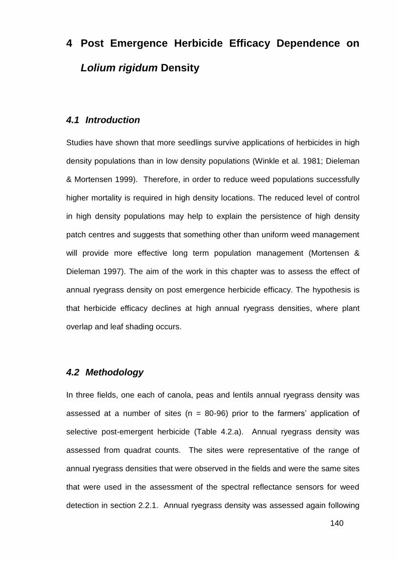
140

4 Post Emergence Herbicide Efficacy Dependence on

Lolium rigidum Density

4.1 Introduction

Studies have shown that more seedlings survive applications of herbicides in high

density populations than in low density populations (Winkle et al. 1981; Dieleman

& Mortensen 1999). Therefore, in order to reduce weed populations successfully

higher mortality is required in high density locations. The reduced level of control

in high density populations may help to explain the persistence of high density

patch centres and suggests that something other than uniform weed management

will provide more effective long term population management (Mortensen &

Dieleman 1997). The aim of the work in this chapter was to assess the effect of

annual ryegrass density on post emergence herbicide efficacy. The hypothesis is

that herbicide efficacy declines at high annual ryegrass densities, where plant

overlap and leaf shading occurs.

4.2 Methodology

In three fields, one each of canola, peas and lentils annual ryegrass density was

assessed at a number of sites (n = 80-96) prior to the farmers’ application of

selective post-emergent herbicide (Table 4.2.a). Annual ryegrass density was

assessed from quadrat counts. The sites were representative of the range of

annual ryegrass densities that were observed in the fields and were the same sites

that were used in the assessment of the spectral reflectance sensors for weed

detection in section 2.2.1. Annual ryegrass density was assessed again following

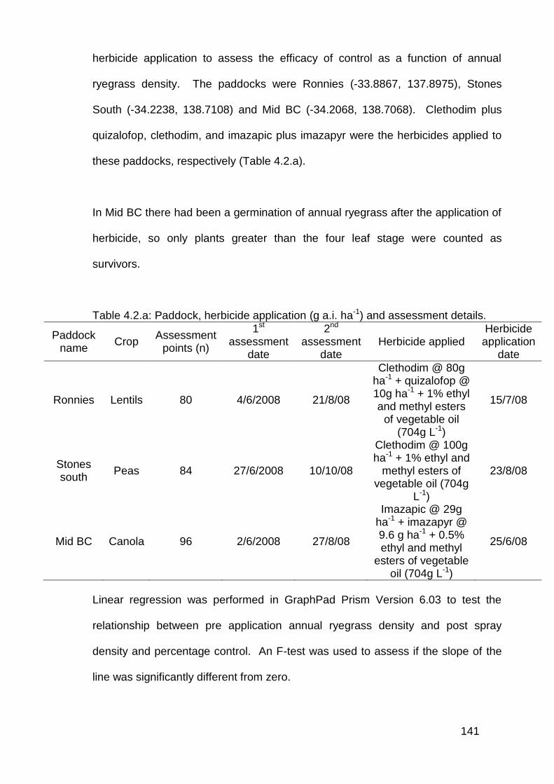
141

herbicide application to assess the efficacy of control as a function of annual

ryegrass density. The paddocks were Ronnies (-33.8867, 137.8975), Stones

South (-34.2238, 138.7108) and Mid BC (-34.2068, 138.7068). Clethodim plus

quizalofop, clethodim, and imazapic plus imazapyr were the herbicides applied to

these paddocks, respectively (Table 4.2.a).

In Mid BC there had been a germination of annual ryegrass after the application of

herbicide, so only plants greater than the four leaf stage were counted as

survivors.

Table 4.2.a: Paddock, herbicide application (g a.i. ha-1) and assessment details.

Paddock name

Crop Assessment

points (n)

1st assessment

date

2nd assessment

date Herbicide applied

Herbicide application

date

Ronnies Lentils 80 4/6/2008 21/8/08

Clethodim @ 80g ha-1 + quizalofop @ 10g ha-1 + 1% ethyl and methyl esters

of vegetable oil (704g L-1)

15/7/08

Stones south

Peas 84 27/6/2008 10/10/08

Clethodim @ 100g ha-1 + 1% ethyl and

methyl esters of vegetable oil (704g

L-1)

23/8/08

Mid BC Canola 96 2/6/2008 27/8/08

Imazapic @ 29g ha-1 + imazapyr @ 9.6 g ha-1 + 0.5% ethyl and methyl

esters of vegetable oil (704g L-1)

25/6/08

Linear regression was performed in GraphPad Prism Version 6.03 to test the

relationship between pre application annual ryegrass density and post spray

density and percentage control. An F-test was used to assess if the slope of the

line was significantly different from zero.

142

4.3 Results

Control of annual ryegrass in Ronnies paddock was between 87 and 100% at all

sites (Figure 4.3.b). Initial densities ranged from 0 to 1600 plants m-2 and after

clethodim plus quizalofop application the densities were reduced to 0 to 18 plants

m-2 (Figure 4.3.a). There is a weak, but significant relationship (R2 = 0.282,

p<0.0001)) between initial density and annual ryegrass density post herbicide

application. Stones South had initial annual ryegrass populations ranging from 0

to 2000 plants m-2 and after clethodim application the population range was 0 to

420 plants m-2 (Figure 4.3.c). The herbicide control was variable, ranging from 0

to 100% (Figure 4.3.d). A positive density relationship between pre and post

clethodim applications is evident (Figure 4.3.c). Mid BC had a large range of

annual ryegrass densities from 0 to 6000 plants m-2 with control ranging from 0 to

100% (Figure 4.3.e and 4.3.f). There is a positive correlation between initial

annual ryegrass population and annual ryegrass surviving imazapic and imazapyr

application in Mid BC (Figure 4.3.e).

The numbers of annual ryegrass plants surviving post-emergence selective

herbicide applications was related to the number of annual ryegrass initially

present, regardless of the herbicide used (Figure 4.3.a, 4.3.c and 4.3.e). Survival

was higher where more annual ryegrass was present at spraying. In Mid BC early

season annual ryegrass density was related to the density of later emerging

cohorts (Figure 4.3.g), where higher density of annual ryegrass early in the season

is correlated with higher emergence density in later cohorts.

The data in these trials suggests that the level of annual ryegrass control is

independent of density (Figure 4.3.b, 4.3.d and 4.3.f). That is, there is no

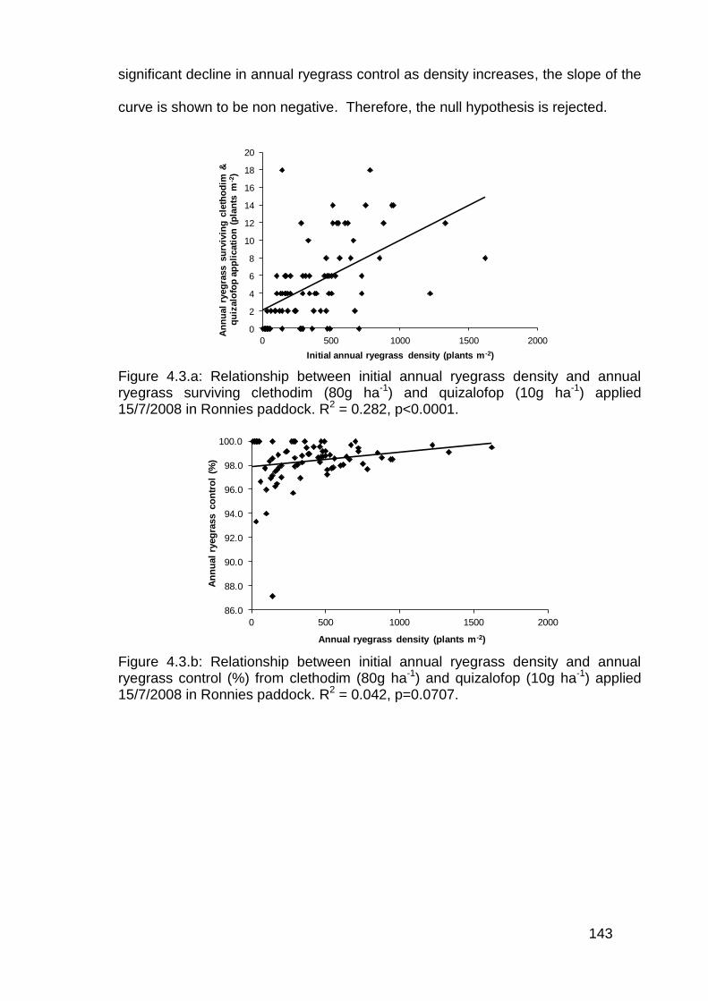
143

significant decline in annual ryegrass control as density increases, the slope of the

curve is shown to be non negative. Therefore, the null hypothesis is rejected.

0

2

4

6

8

10

12

14

16

18

20

0 500 1000 1500 2000

An

nu

al

ryeg

rass s

urv

ivin

g c

leth

od

im &

q

uiz

alo

fop

ap

pli

cati

on

(p

lan

ts m

-2)

Initial annual ryegrass density (plants m -2)

Figure 4.3.a: Relationship between initial annual ryegrass density and annual ryegrass surviving clethodim (80g ha-1) and quizalofop (10g ha-1) applied 15/7/2008 in Ronnies paddock. R2 = 0.282, p<0.0001.

86.0

88.0

90.0

92.0

94.0

96.0

98.0

100.0

0 500 1000 1500 2000

An

nu

al

ryeg

rass c

on

tro

l (%

)

Annual ryegrass density (plants m-2)

Figure 4.3.b: Relationship between initial annual ryegrass density and annual ryegrass control (%) from clethodim (80g ha-1) and quizalofop (10g ha-1) applied 15/7/2008 in Ronnies paddock. R2 = 0.042, p=0.0707.

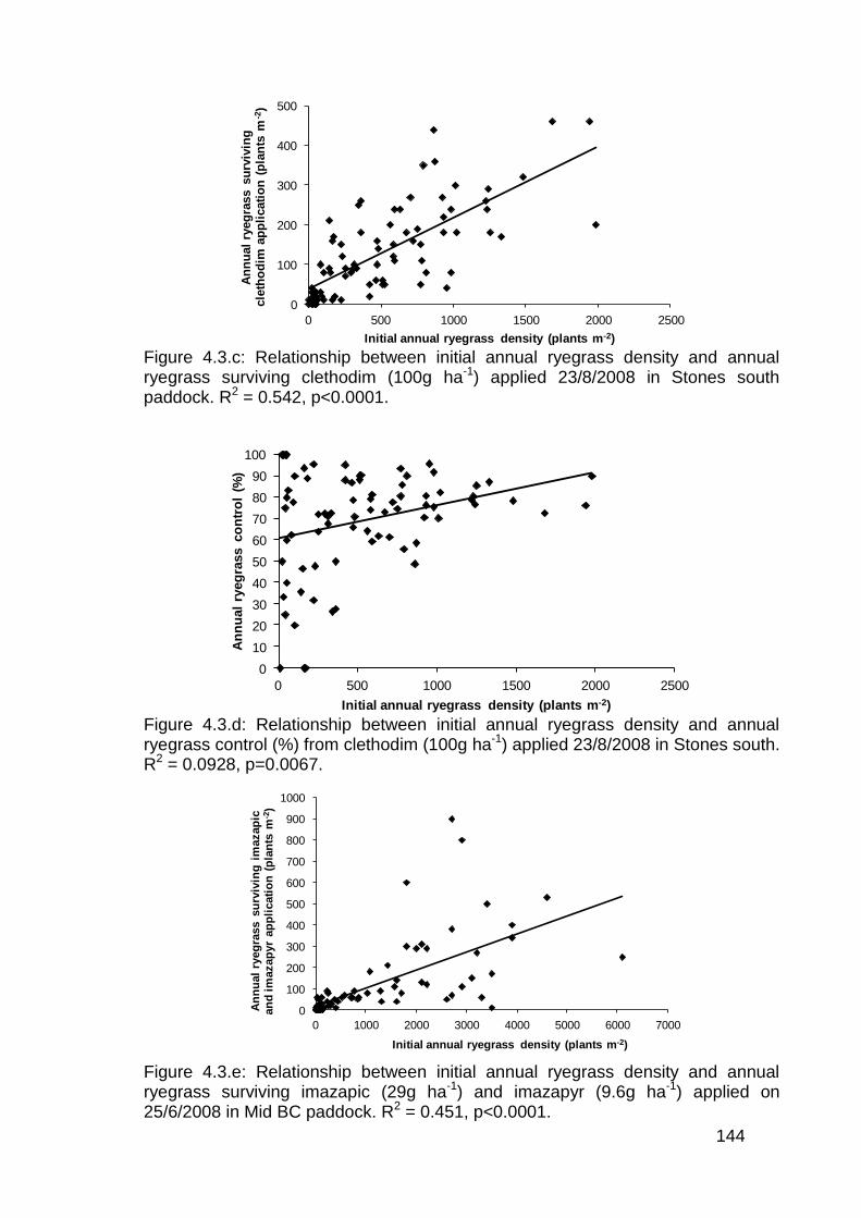
144

0

100

200

300

400

500

0 500 1000 1500 2000 2500

An

nu

al

ryeg

rass s

urv

ivin

g

cle

tho

dim

ap

pli

cati

on

(p

lan

ts m

-2)

Initial annual ryegrass density (plants m-2) Figure 4.3.c: Relationship between initial annual ryegrass density and annual ryegrass surviving clethodim (100g ha-1) applied 23/8/2008 in Stones south paddock. R2 = 0.542, p<0.0001.

0

10

20

30

40

50

60

70

80

90

100

0 500 1000 1500 2000 2500

An

nu

al

ryeg

rass c

on

tro

l (%

)

Initial annual ryegrass density (plants m-2) Figure 4.3.d: Relationship between initial annual ryegrass density and annual ryegrass control (%) from clethodim (100g ha-1) applied 23/8/2008 in Stones south. R2 = 0.0928, p=0.0067.

0

100

200

300

400

500

600

700

800

900

1000

0 1000 2000 3000 4000 5000 6000 7000

An

nu

al

ryeg

rass s

urv

ivin

g i

mazap

ic

an

d im

azap

yr

ap

pli

cati

on

(p

lan

ts m

-2)

Initial annual ryegrass density (plants m-2)

Figure 4.3.e: Relationship between initial annual ryegrass density and annual ryegrass surviving imazapic (29g ha-1) and imazapyr (9.6g ha-1) applied on 25/6/2008 in Mid BC paddock. R2 = 0.451, p<0.0001.

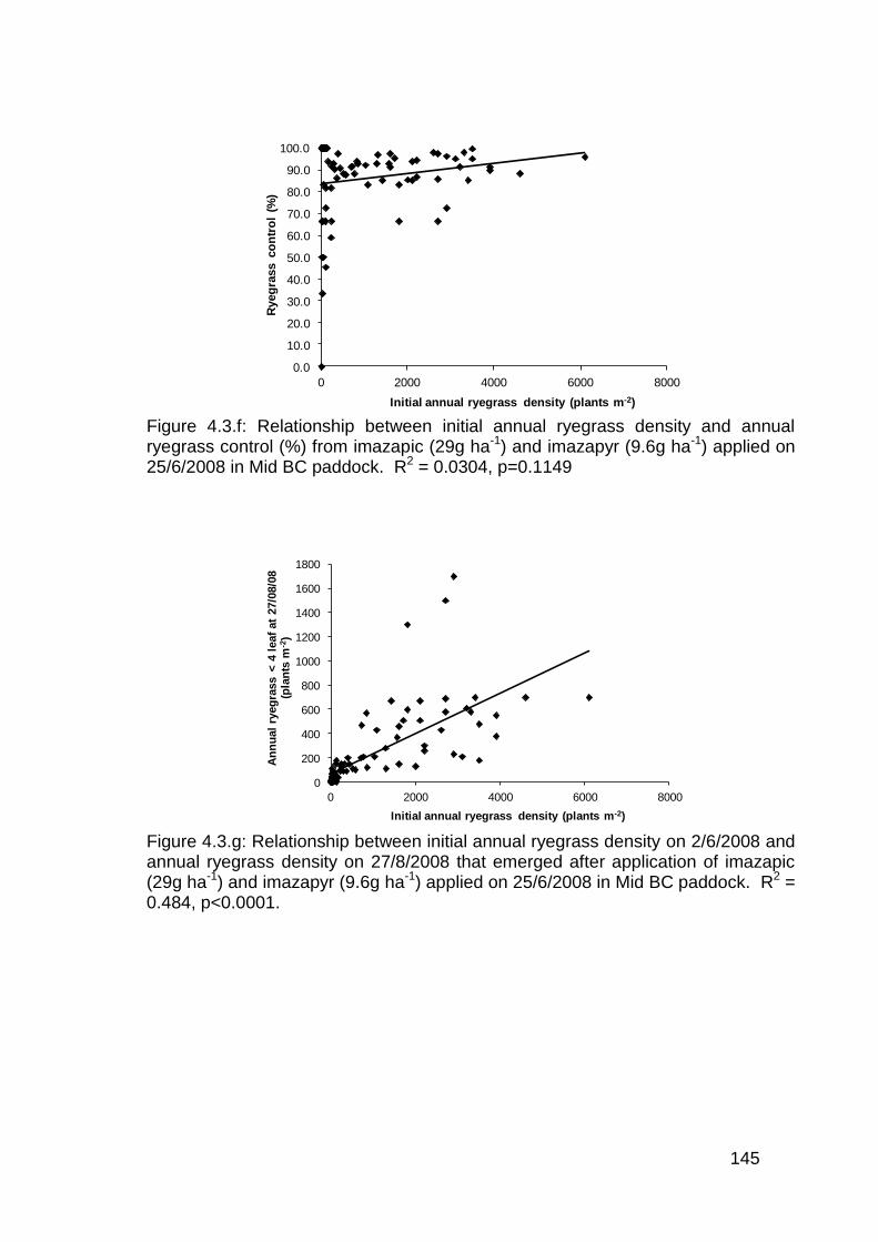
145

0.0

10.0

20.0

30.0

40.0

50.0

60.0

70.0

80.0

90.0

100.0

0 2000 4000 6000 8000

Ryeg

rass c

on

tro

l (%

)

Initial annual ryegrass density (plants m-2)

Figure 4.3.f: Relationship between initial annual ryegrass density and annual ryegrass control (%) from imazapic (29g ha-1) and imazapyr (9.6g ha-1) applied on 25/6/2008 in Mid BC paddock. R2 = 0.0304, p=0.1149

0

200

400

600

800

1000

1200

1400

1600

1800

0 2000 4000 6000 8000

An

nu

al

ryeg

rass <

4 l

eaf

at

27/0

8/0

8

(pla

nts

m-2

)

Initial annual ryegrass density (plants m-2)

Figure 4.3.g: Relationship between initial annual ryegrass density on 2/6/2008 and annual ryegrass density on 27/8/2008 that emerged after application of imazapic (29g ha-1) and imazapyr (9.6g ha-1) applied on 25/6/2008 in Mid BC paddock. R2 = 0.484, p<0.0001.

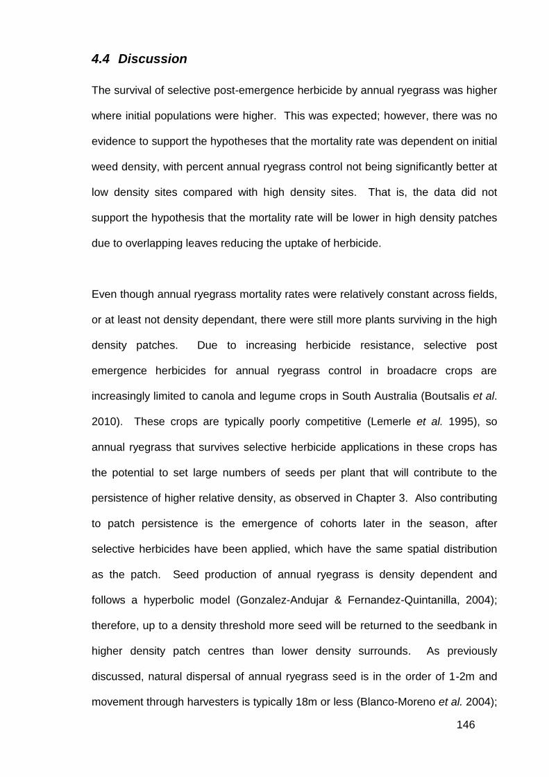
146

4.4 Discussion

The survival of selective post-emergence herbicide by annual ryegrass was higher

where initial populations were higher. This was expected; however, there was no

evidence to support the hypotheses that the mortality rate was dependent on initial

weed density, with percent annual ryegrass control not being significantly better at

low density sites compared with high density sites. That is, the data did not

support the hypothesis that the mortality rate will be lower in high density patches

due to overlapping leaves reducing the uptake of herbicide.

Even though annual ryegrass mortality rates were relatively constant across fields,

or at least not density dependant, there were still more plants surviving in the high

density patches. Due to increasing herbicide resistance, selective post

emergence herbicides for annual ryegrass control in broadacre crops are

increasingly limited to canola and legume crops in South Australia (Boutsalis et al.

2010). These crops are typically poorly competitive (Lemerle et al. 1995), so

annual ryegrass that survives selective herbicide applications in these crops has

the potential to set large numbers of seeds per plant that will contribute to the

persistence of higher relative density, as observed in Chapter 3. Also contributing

to patch persistence is the emergence of cohorts later in the season, after

selective herbicides have been applied, which have the same spatial distribution

as the patch. Seed production of annual ryegrass is density dependent and

follows a hyperbolic model (Gonzalez-Andujar & Fernandez-Quintanilla, 2004);

therefore, up to a density threshold more seed will be returned to the seedbank in

higher density patch centres than lower density surrounds. As previously

discussed, natural dispersal of annual ryegrass seed is in the order of 1-2m and

movement through harvesters is typically 18m or less (Blanco-Moreno et al. 2004);

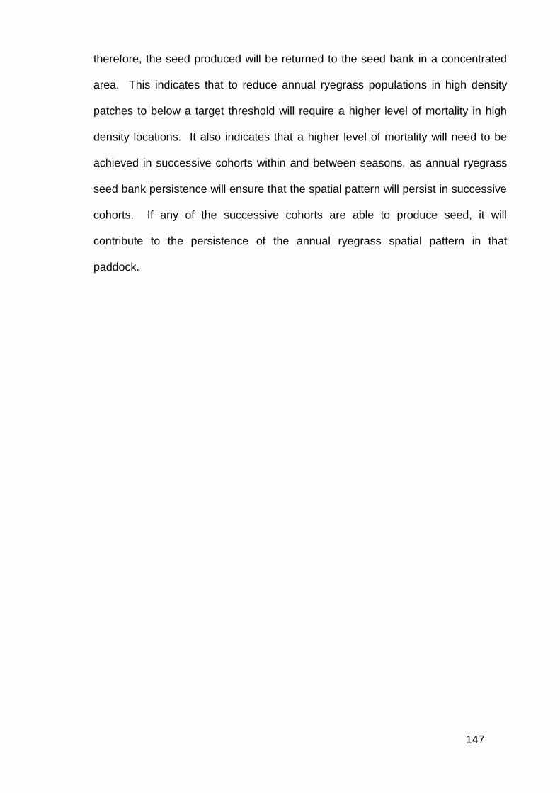
147

therefore, the seed produced will be returned to the seed bank in a concentrated

area. This indicates that to reduce annual ryegrass populations in high density

patches to below a target threshold will require a higher level of mortality in high

density locations. It also indicates that a higher level of mortality will need to be

achieved in successive cohorts within and between seasons, as annual ryegrass

seed bank persistence will ensure that the spatial pattern will persist in successive

cohorts. If any of the successive cohorts are able to produce seed, it will

contribute to the persistence of the annual ryegrass spatial pattern in that

paddock.

148

5 Herbicide Treatment Options for Patch Management of

Lolium rigidum and their Economic Implications

5.1 Introduction

Herbicides tend to be the most widely used weed control tactic. A study by

Llewellyn et al. (2004) reports that grain growers perceive herbicide-based weed

control practices as the most cost-effective. However, annual ryegrass continues

to develop resistance and multiple resistances to a range of herbicides and for this

reason it is considered among the most important examples of economic

disruption due to herbicide resistance in world agriculture (Broster & Pratley 2006).

Herbicide resistance development in annual ryegrass has left many farmers with

only a couple of herbicide options, those being the use of pre-emergent herbicides

in cereals and the use of selective group A herbicides in broad leaf crops

(Boutsalis et al. 2010).

SSWM requires the determination of the correct herbicide dose to apply to patch

and non-patch areas and implies that there is a target weed density to be achieved

through applying the herbicide and a known dose response curve from which a

rate can be selected to achieve the desired efficacy. However, factors such as

weed size, density, age, stress and history can influence herbicide efficacy and

can make herbicide dose response difficult to predict (Thorp & Tian 2004a).

Variability in soil conditions can also influence the bioactivity of soil applied

herbicides (Blumhorst et al. 1990).

149

The most common benefit cited for SSWM is that of herbicide savings. Herbicide

savings are generally reported as the amount of herbicide used to spray the weed

patches compared with what would have been required to treat the whole paddock

with a uniform 100% rate. Herbicide savings tend to be greater for on/off (spray/no

spray) treatment decisions than high dose/low dose treatments. However, the

former is considered more risky as untreated patches have the potential for weed

escapes to contribute seed to the seed bank and create problems for future

seasons (Rew et al. 1996; Lutman & Miller 2007).

In addition to implementing SSWM for the sole purpose of herbicide savings,

targeting more intensive weed control strategies in high density patches of hard-to-

control weeds, such as annual ryegrass, could prove beneficial in southern

Australian cropping systems. The aim of these experiments is to assess the

opportunities for variable rate application of herbicides for improved weed

management and economic outcomes.

5.2 Methodology

5.2.1 Post emergence herbicide trials in lentils

5.2.1.1 Pig paddock clethodim trial

Two trials were established in lentils growing in Pig paddock (-33.8782, 138.0772)

assessing the efficacy of clethodim (240g a.i. L-1) in high and low density annual

ryegrass populations in 2007. High and low density populations were identified by

field scouting. The trials were a completely randomised block design with five

replicates. Treatments and treatment costs are shown in Table 5.2.1.1.a.

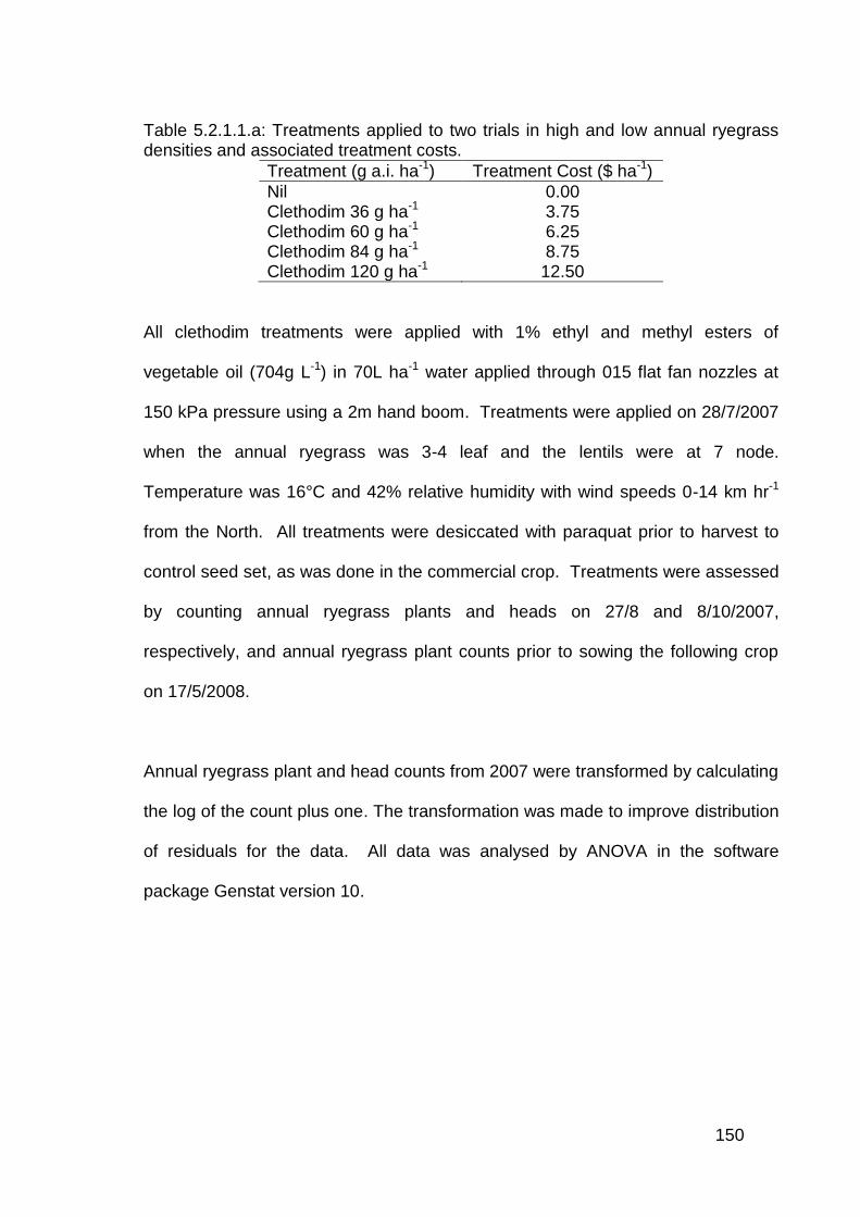
150

Table 5.2.1.1.a: Treatments applied to two trials in high and low annual ryegrass densities and associated treatment costs.

Treatment (g a.i. ha-1) Treatment Cost ($ ha-1)

Nil 0.00 Clethodim 36 g ha-1 3.75 Clethodim 60 g ha-1 6.25 Clethodim 84 g ha-1 8.75 Clethodim 120 g ha-1 12.50

All clethodim treatments were applied with 1% ethyl and methyl esters of

vegetable oil (704g L-1) in 70L ha-1 water applied through 015 flat fan nozzles at

150 kPa pressure using a 2m hand boom. Treatments were applied on 28/7/2007

when the annual ryegrass was 3-4 leaf and the lentils were at 7 node.

Temperature was 16°C and 42% relative humidity with wind speeds 0-14 km hr-1

from the North. All treatments were desiccated with paraquat prior to harvest to

control seed set, as was done in the commercial crop. Treatments were assessed

by counting annual ryegrass plants and heads on 27/8 and 8/10/2007,

respectively, and annual ryegrass plant counts prior to sowing the following crop

on 17/5/2008.

Annual ryegrass plant and head counts from 2007 were transformed by calculating

the log of the count plus one. The transformation was made to improve distribution

of residuals for the data. All data was analysed by ANOVA in the software

package Genstat version 10.

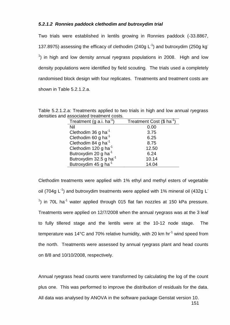
151

5.2.1.2 Ronnies paddock clethodim and butroxydim trial

Two trials were established in lentils growing in Ronnies paddock (-33.8867,

137.8975) assessing the efficacy of clethodim (240g L-1) and butroxydim (250g kg-

1) in high and low density annual ryegrass populations in 2008. High and low

density populations were identified by field scouting. The trials used a completely

randomised block design with four replicates. Treatments and treatment costs are

shown in Table 5.2.1.2.a.

Table 5.2.1.2.a: Treatments applied to two trials in high and low annual ryegrass densities and associated treatment costs.

Treatment (g a.i. ha-1) Treatment Cost ($ ha-1)

Nil 0.00 Clethodim 36 g ha-1 3.75 Clethodim 60 g ha-1 6.25 Clethodim 84 g ha-1 8.75 Clethodim 120 g ha-1 12.50 Butroxydim 20 g ha-1 6.24 Butroxydim 32.5 g ha-1 10.14 Butroxydim 45 g ha-1 14.04

Clethodim treatments were applied with 1% ethyl and methyl esters of vegetable

oil (704g L-1) and butroxydim treatments were applied with 1% mineral oil (432g L-

1) in 70L ha-1 water applied through 015 flat fan nozzles at 150 kPa pressure.

Treatments were applied on 12/7/2008 when the annual ryegrass was at the 3 leaf

to fully tillered stage and the lentils were at the 10-12 node stage. The

temperature was 14°C and 70% relative humidity, with 20 km hr-1 wind speed from

the north. Treatments were assessed by annual ryegrass plant and head counts

on 8/8 and 10/10/2008, respectively.

Annual ryegrass head counts were transformed by calculating the log of the count

plus one. This was performed to improve the distribution of residuals for the data.

All data was analysed by ANOVA in the software package Genstat version 10.

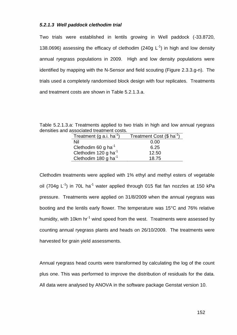
152

5.2.1.3 Well paddock clethodim trial

Two trials were established in lentils growing in Well paddock (-33.8720,

138.0696) assessing the efficacy of clethodim (240g L-1) in high and low density

annual ryegrass populations in 2009. High and low density populations were

identified by mapping with the N-Sensor and field scouting (Figure 2.3.3.g-n). The

trials used a completely randomised block design with four replicates. Treatments

and treatment costs are shown in Table 5.2.1.3.a.

Table 5.2.1.3.a: Treatments applied to two trials in high and low annual ryegrass densities and associated treatment costs.

Treatment (g a.i. ha-1) Treatment Cost ($ ha-1)

Nil 0.00 Clethodim 60 g ha-1 6.25 Clethodim 120 g ha-1 12.50 Clethodim 180 g ha-1 18.75

Clethodim treatments were applied with 1% ethyl and methyl esters of vegetable

oil (704g L-1) in 70L ha-1 water applied through 015 flat fan nozzles at 150 kPa

pressure. Treatments were applied on 31/8/2009 when the annual ryegrass was

booting and the lentils early flower. The temperature was 15°C and 76% relative

humidity, with 10km hr-1 wind speed from the west. Treatments were assessed by

counting annual ryegrass plants and heads on 26/10/2009. The treatments were

harvested for grain yield assessments.

Annual ryegrass head counts were transformed by calculating the log of the count

plus one. This was performed to improve the distribution of residuals for the data.

All data were analysed by ANOVA in the software package Genstat version 10.

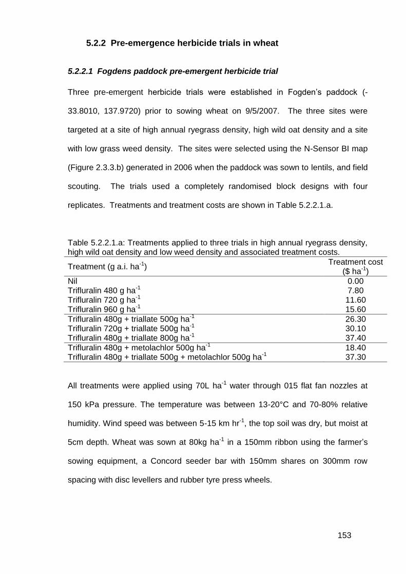
153

5.2.2 Pre-emergence herbicide trials in wheat

5.2.2.1 Fogdens paddock pre-emergent herbicide trial

Three pre-emergent herbicide trials were established in Fogden’s paddock (-

33.8010, 137.9720) prior to sowing wheat on 9/5/2007. The three sites were

targeted at a site of high annual ryegrass density, high wild oat density and a site

with low grass weed density. The sites were selected using the N-Sensor BI map

(Figure 2.3.3.b) generated in 2006 when the paddock was sown to lentils, and field

scouting. The trials used a completely randomised block designs with four

replicates. Treatments and treatment costs are shown in Table 5.2.2.1.a.

Table 5.2.2.1.a: Treatments applied to three trials in high annual ryegrass density, high wild oat density and low weed density and associated treatment costs.

Treatment (g a.i. ha-1) Treatment cost

($ ha-1)

Nil 0.00 Trifluralin 480 g ha-1 7.80 Trifluralin 720 g ha-1 11.60 Trifluralin 960 g ha-1 15.60

Trifluralin 480g + triallate 500g ha-1 26.30 Trifluralin 720g + triallate 500g ha-1 30.10 Trifluralin 480g + triallate 800g ha-1 37.40

Trifluralin 480g + metolachlor 500g ha-1 18.40 Trifluralin 480g + triallate 500g + metolachlor 500g ha-1 37.30

All treatments were applied using 70L ha-1 water through 015 flat fan nozzles at

150 kPa pressure. The temperature was between 13-20°C and 70-80% relative

humidity. Wind speed was between 5-15 km hr-1, the top soil was dry, but moist at

5cm depth. Wheat was sown at 80kg ha-1 in a 150mm ribbon using the farmer’s

sowing equipment, a Concord seeder bar with 150mm shares on 300mm row

spacing with disc levellers and rubber tyre press wheels.

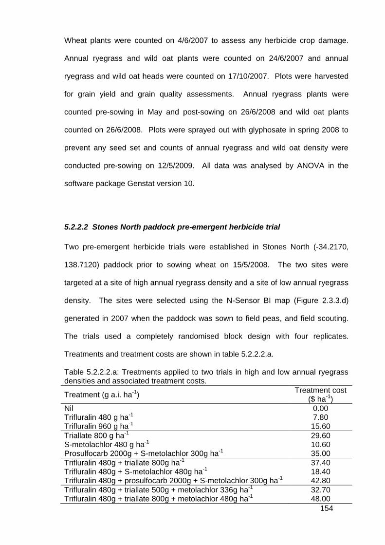
154

Wheat plants were counted on 4/6/2007 to assess any herbicide crop damage.

Annual ryegrass and wild oat plants were counted on 24/6/2007 and annual

ryegrass and wild oat heads were counted on 17/10/2007. Plots were harvested

for grain yield and grain quality assessments. Annual ryegrass plants were

counted pre-sowing in May and post-sowing on 26/6/2008 and wild oat plants

counted on 26/6/2008. Plots were sprayed out with glyphosate in spring 2008 to

prevent any seed set and counts of annual ryegrass and wild oat density were

conducted pre-sowing on 12/5/2009. All data was analysed by ANOVA in the

software package Genstat version 10.

5.2.2.2 Stones North paddock pre-emergent herbicide trial

Two pre-emergent herbicide trials were established in Stones North (-34.2170,

138.7120) paddock prior to sowing wheat on 15/5/2008. The two sites were

targeted at a site of high annual ryegrass density and a site of low annual ryegrass

density. The sites were selected using the N-Sensor BI map (Figure 2.3.3.d)

generated in 2007 when the paddock was sown to field peas, and field scouting.

The trials used a completely randomised block design with four replicates.

Treatments and treatment costs are shown in table 5.2.2.2.a.

Table 5.2.2.2.a: Treatments applied to two trials in high and low annual ryegrass densities and associated treatment costs.

Treatment (g a.i. ha-1) Treatment cost

($ ha-1)

Nil 0.00 Trifluralin 480 g ha-1 7.80 Trifluralin 960 g ha-1 15.60

Triallate 800 g ha-1 29.60 S-metolachlor 480 g ha-1 10.60 Prosulfocarb 2000g + S-metolachlor 300g ha-1 35.00

Trifluralin 480g + triallate 800g ha-1 37.40 Trifluralin 480g + S-metolachlor 480g ha-1 18.40 Trifluralin 480g + prosulfocarb 2000g + S-metolachlor 300g ha-1 42.80

Trifluralin 480g + triallate 500g + metolachlor 336g ha-1 32.70 Trifluralin 480g + triallate 800g + metolachlor 480g ha-1 48.00

155

All treatments were applied using 70L ha-1 water through 015 flat fan nozzles at

150 kPa pressure. The temperature was 23°C and 35% relative humidity and 13-

16 km hr-1 wind speed from the north-west. The top soil was dry, but soil was

moist at 5cm. Wheat was sown at 90kg ha-1 using the farmer’s sowing equipment,

a Horwood Bagshaw seeder bar with knife points on 225mm row spacing, with

press wheels.

Wheat plants were counted on 13/6/2008 to assess any herbicide crop damage.

Annual ryegrass plants were counted on 25/6/2008 and annual ryegrass heads

were counted on 27/11/2008. Plots were harvested for grain yield and grain

quality assessments. Annual ryegrass plants were counted on 20/5/2009. All data

was analysed by ANOVA in the software package Genstat version 10.

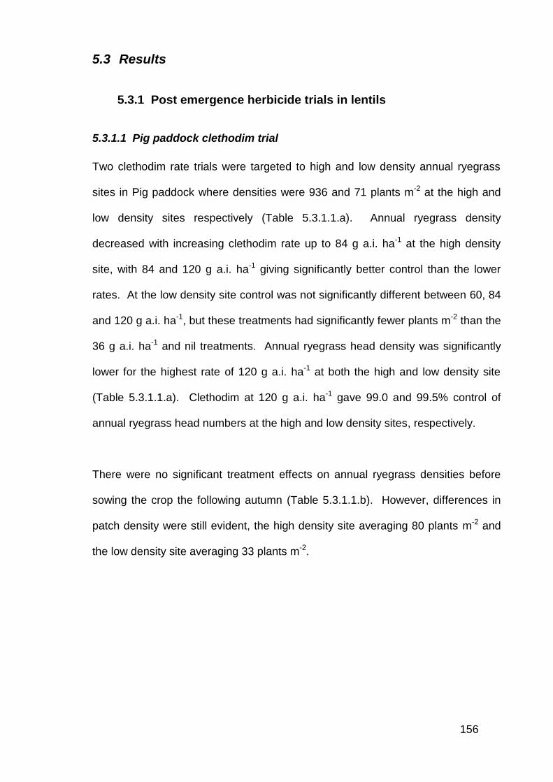
156

5.3 Results

5.3.1 Post emergence herbicide trials in lentils

5.3.1.1 Pig paddock clethodim trial

Two clethodim rate trials were targeted to high and low density annual ryegrass

sites in Pig paddock where densities were 936 and 71 plants m-2 at the high and

low density sites respectively (Table 5.3.1.1.a). Annual ryegrass density

decreased with increasing clethodim rate up to 84 g a.i. ha-1 at the high density

site, with 84 and 120 g a.i. ha-1 giving significantly better control than the lower

rates. At the low density site control was not significantly different between 60, 84

and 120 g a.i. ha-1, but these treatments had significantly fewer plants m-2 than the

36 g a.i. ha-1 and nil treatments. Annual ryegrass head density was significantly

lower for the highest rate of 120 g a.i. ha-1 at both the high and low density site

(Table 5.3.1.1.a). Clethodim at 120 g a.i. ha-1 gave 99.0 and 99.5% control of

annual ryegrass head numbers at the high and low density sites, respectively.

There were no significant treatment effects on annual ryegrass densities before

sowing the crop the following autumn (Table 5.3.1.1.b). However, differences in

patch density were still evident, the high density site averaging 80 plants m-2 and

the low density site averaging 33 plants m-2.

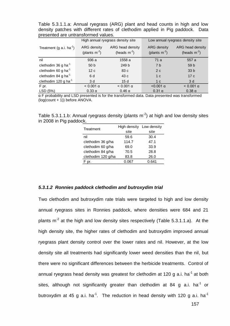
157

Table 5.3.1.1.a: Annual ryegrass (ARG) plant and head counts in high and low density patches with different rates of clethodim applied in Pig paddock. Data presented are untransformed values.

ARG density

(plants m-2)

ARG head density

(heads m-2)

ARG density

(plants m-2)

ARG head density

(heads m-2)

nil 936 a 1558 a 71 a 557 a

clethodim 36 g ha-1 50 b 249 b 7 b 59 b

clethodim 60 g ha-1 12 c 83 c 2 c 33 b

clethodim 84 g ha-1 6 d 43 c 1 c 17 c

clethodim 120 g ha-1 3 d 15 d 1 c 3 d

F pr. < 0.001 α < 0.001 α <0.001 α < 0.001 α

LSD (5%) 0.33 α 0.46 α 0.31 α 0.3 α

High annual ryegrass density site Low annual ryegrass density site

Treatment (g a.i. ha-1)

α F probability and LSD presented is for the transformed data. Data presented was transformed (log(count + 1)) before ANOVA.

Table 5.3.1.1.b: Annual ryegrass density (plants m-2) at high and low density sites in 2008 in Pig paddock.

TreatmentHigh density

site

Low density

site

nil 59.6 30.4

clethodim 36 g/ha 114.7 47.1

clethodim 60 g/ha 69.0 33.9

clethodim 84 g/ha 70.5 28.8

clethodim 120 g/ha 83.8 26.0

F pr. 0.067 0.641

5.3.1.2 Ronnies paddock clethodim and butroxydim trial

Two clethodim and butroxydim rate trials were targeted to high and low density

annual ryegrass sites in Ronnies paddock, where densities were 684 and 21

plants m-2 at the high and low density sites respectively (Table 5.3.1.1.a). At the

high density site, the higher rates of clethodim and butroxydim improved annual

ryegrass plant density control over the lower rates and nil. However, at the low

density site all treatments had significantly lower weed densities than the nil, but

there were no significant differences between the herbicide treatments. Control of

annual ryegrass head density was greatest for clethodim at 120 g a.i. ha-1 at both

sites, although not significantly greater than clethodim at 84 g a.i. ha-1 or

butroxydim at 45 g a.i. ha-1. The reduction in head density with 120 g a.i. ha-1

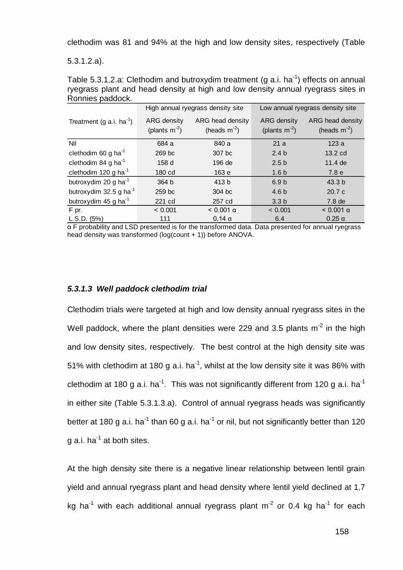
158

clethodim was 81 and 94% at the high and low density sites, respectively (Table

5.3.1.2.a).

Table 5.3.1.2.a: Clethodim and butroxydim treatment (g a.i. ha-1) effects on annual ryegrass plant and head density at high and low density annual ryegrass sites in Ronnies paddock.

ARG density

(plants m-2)

ARG head density

(heads m-2)

ARG density

(plants m-2)

ARG head density

(heads m-2)

Nil 684 a 840 a 21 a 123 a

clethodim 60 g ha-1 269 bc 307 bc 2.4 b 13.2 cd

clethodim 84 g ha-1 158 d 196 de 2.5 b 11.4 de

clethodim 120 g ha-1 180 cd 163 e 1.6 b 7.8 e

butroxydim 20 g ha-1 364 b 413 b 6.9 b 43.3 b

butroxydim 32.5 g ha-1 259 bc 304 bc 4.6 b 20.7 c

butroxydim 45 g ha-1 221 cd 257 cd 3.3 b 7.8 de

F pr. < 0.001 < 0.001 α < 0.001 < 0.001 α

L.S.D. (5%) 111 0.14 α 6.4 0.2 α

Treatment (g a.i. ha-1)

High annual ryegrass density site Low annual ryegrass density site

α F probability and LSD presented is for the transformed data. Data presented for annual ryegrass head density was transformed (log(count + 1)) before ANOVA.

5.3.1.3 Well paddock clethodim trial

Clethodim trials were targeted at high and low density annual ryegrass sites in the

Well paddock, where the plant densities were 229 and 3.5 plants m-2 in the high

and low density sites, respectively. The best control at the high density site was

51% with clethodim at 180 g a.i. ha-1, whilst at the low density site it was 86% with

clethodim at 180 g a.i. ha-1. This was not significantly different from 120 g a.i. ha-1

in either site (Table 5.3.1.3.a). Control of annual ryegrass heads was significantly

better at 180 g a.i. ha-1 than 60 g a.i. ha-1 or nil, but not significantly better than 120

g a.i. ha-1 at both sites.

At the high density site there is a negative linear relationship between lentil grain

yield and annual ryegrass plant and head density where lentil yield declined at 1.7

kg ha-1 with each additional annual ryegrass plant m-2 or 0.4 kg ha-1 for each

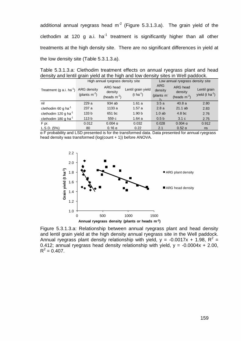
159

additional annual ryegrass head m-2 (Figure 5.3.1.3.a). The grain yield of the

clethodim at 120 g a.i. ha-1 treatment is significantly higher than all other

treatments at the high density site. There are no significant differences in yield at

the low density site (Table 5.3.1.3.a).

Table 5.3.1.3.a: Clethodim treatment effects on annual ryegrass plant and head density and lentil grain yield at the high and low density sites in Well paddock.

ARG density

(plants m-2)

ARG head

density

(heads m-2)

Lentil grain yield

(t ha-1)

ARG

density

(plants m-

2)

ARG head

density

(heads m-2)

Lentil grain

yield (t ha-1)

nil 229 a 934 ab 1.61 a 3.5 a 40.8 a 2.80

clethodim 60 g ha-1 237 a 1133 a 1.57 a 2.8 a 21.1 ab 2.83

clethodim 120 g ha-1 133 b 651 bc 1.90 b 1.0 ab 4.8 bc 2.76

clethodim 180 g ha-1 113 b 559 c 1.64 a 0.5 b 3.1 c 2.75

F pr. 0.012 0.004 α 0.032 0.028 0.004 α 0.912

L.S.D. (5%) 80 0.16 α 0.22 2.1 0. 2 α ns

Treatment (g a.i. ha-1)

High annual ryegrass density site Low annual ryegrass density site

α F probability and LSD presented is for the transformed data. Data presented for annual ryegrass head density was transformed (log(count + 1)) before ANOVA.

1.0

1.2

1.4

1.6

1.8

2.0

2.2

0 500 1000 1500

Gra

in y

ield

(t

ha

-1)

Annual ryegrass density (plants or heads m-2)

ARG plant density

ARG head density

Figure 5.3.1.3.a: Relationship between annual ryegrass plant and head density and lentil grain yield at the high density annual ryegrass site in the Well paddock. Annual ryegrass plant density relationship with yield, y = -0.0017x + 1.98, R2 = 0.412; annual ryegrass head density relationship with yield, y = -0.0004x + 2.00, R2 = 0.407.

160

5.3.2 Pre-emergent herbicide trials in wheat

5.3.2.1 Fogdens paddock pre-emergent herbicide trial

Three trial sites were targeted to three weed density types, including high annual

ryegrass density, high wild oat density and low weed density situations in season

2007. The weed densities at these sites were 574 annual ryegrass plants m-2 at

the high density annual ryegrass site, 11 annual ryegrass plants m-2 at the low

density annual ryegrass site and 557 wild oat plants m-2 at the high density wild

oat site. At the high density annual ryegrass site, annual ryegrass control was

poor where trifluralin was used alone, achieving less than 50% control at rates up

to 960 g a.i. ha-1 (Figure 5.3.2.1.a). Annual ryegrass control was improved

significantly at this site with the addition of triallate to trifluralin, at either 500 or 800

g ha-1, improving control by between 24 and 64% over trifluralin used alone. The

addition of 500 g a.i. ha-1 metolachlor to 480 g a.i. ha-1 trifluralin improved control

by 44%. The combination of trifluralin, triallate and metolachlor resulted in the

greatest population reduction, reducing it to 20% of the untreated. However, this

was not significantly different from the trifluralin and triallate mixes (Figure

5.3.2.1.a). Similar trends were observed in annual ryegrass head density at the

high ryegrass site (Figure 5.3.2.1.b). At all sites there was a significant reduction

in populations during the season, with weed head densities being approximately

one third of the in-season plant density.

At the low annual ryegrass density site, all herbicides significantly reduced the

annual ryegrass density by more than 50% compared with the untreated.

However, there was little difference between treatments (Figure 5.3.2.1.a),

although low rates of trifluralin used on their own tended to provide poorer control.

161

There were no significant differences between any treatments for head densities at

the low density annual ryegrass site (Figure 5.3.2.1.b).

At the high density wild oat site all treatments significantly reduced wild oat plant

and head densities (Figure 5.3.2.1.a & 5.3.2.1.b). There is a trend towards

improved control with the highest rate of trifluralin, and the addition of triallate and

metolachlor also tends to improve control, but these differences are not significant.

A negative regression between wild oat head density and grain yield was observed

at the high wild oat site (Figure 5.3.2.1.c), where 2 kg ha-1 grain yield was lost for

each additional wild oat head m-2. However, no similar trends were observed in

relation to annual ryegrass density at the other sites. As a result, grain yield

differences in response to herbicide treatment were significant at the high wild oat

site, but not at the high and low density annual ryegrass sites (Figure 5.3.2.1.d).

In particular, at the high density wild oat site, the nil treatment yielded significantly

less than all other treatments, and the mix of trifluralin, triallate and metolachlor

yielded significantly more than all other herbicide treatments.

Wheat harvested from the low density weed site had significantly higher protein

content than from the high density weed sites. The differences were large enough

that wheat harvested from the low density site would have been classified as

Australian Hard (H1), the high density wild oat site as Australian Premium White

(APW1) and the high density annual ryegrass site as Australian Standard White

(ASW1) (Figure 5.3.2.1.e).

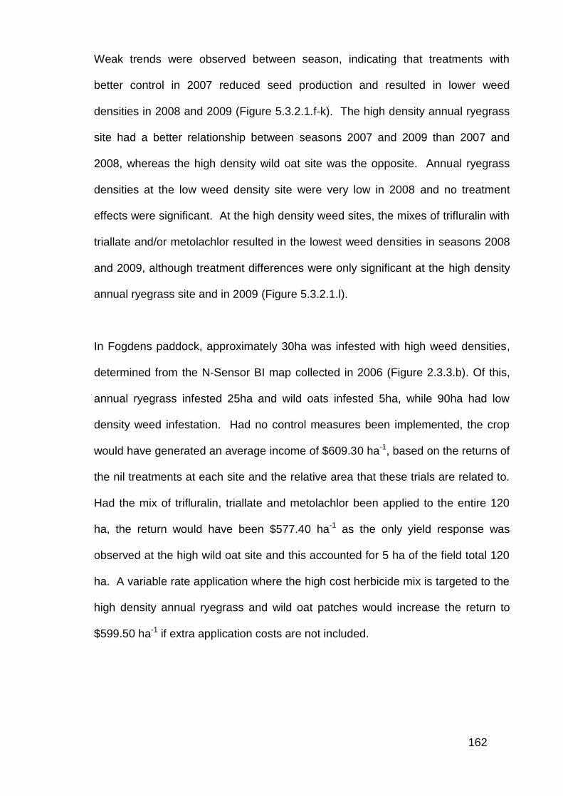
162

Weak trends were observed between season, indicating that treatments with

better control in 2007 reduced seed production and resulted in lower weed

densities in 2008 and 2009 (Figure 5.3.2.1.f-k). The high density annual ryegrass

site had a better relationship between seasons 2007 and 2009 than 2007 and

2008, whereas the high density wild oat site was the opposite. Annual ryegrass

densities at the low weed density site were very low in 2008 and no treatment

effects were significant. At the high density weed sites, the mixes of trifluralin with

triallate and/or metolachlor resulted in the lowest weed densities in seasons 2008

and 2009, although treatment differences were only significant at the high density

annual ryegrass site and in 2009 (Figure 5.3.2.1.l).

In Fogdens paddock, approximately 30ha was infested with high weed densities,

determined from the N-Sensor BI map collected in 2006 (Figure 2.3.3.b). Of this,

annual ryegrass infested 25ha and wild oats infested 5ha, while 90ha had low

density weed infestation. Had no control measures been implemented, the crop

would have generated an average income of $609.30 ha-1, based on the returns of

the nil treatments at each site and the relative area that these trials are related to.

Had the mix of trifluralin, triallate and metolachlor been applied to the entire 120

ha, the return would have been $577.40 ha-1 as the only yield response was

observed at the high wild oat site and this accounted for 5 ha of the field total 120

ha. A variable rate application where the high cost herbicide mix is targeted to the

high density annual ryegrass and wild oat patches would increase the return to

$599.50 ha-1 if extra application costs are not included.

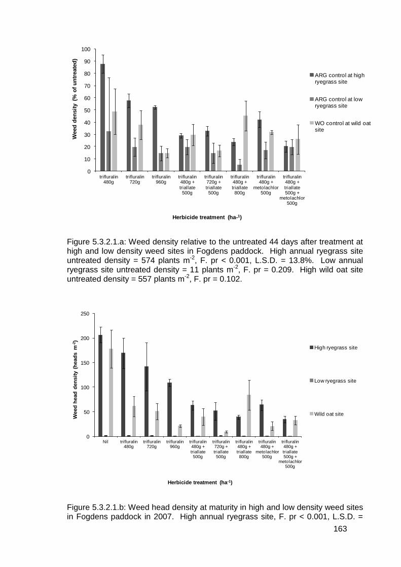
163

0

10

20

30

40

50

60

70

80

90

100

trifluralin 480g

trifluralin 720g

trifluralin 960g

trifluralin 480g +

triallate 500g

trifluralin 720g +

triallate 500g

trifluralin 480g +

triallate 800g

trifluralin 480g +

metolachlor 500g

trifluralin 480g +

triallate 500g +

metolachlor 500g

Weed

den

sit

y (

% o

f u

ntr

eate

d)

Herbicide treatment (ha-1)

ARG control at high ryegrass site

ARG control at low ryegrass site

WO control at wild oat site

Figure 5.3.2.1.a: Weed density relative to the untreated 44 days after treatment at high and low density weed sites in Fogdens paddock. High annual ryegrass site untreated density = 574 plants m-2, F. pr < 0.001, L.S.D. = 13.8%. Low annual ryegrass site untreated density = 11 plants m-2, F. pr = 0.209. High wild oat site untreated density = 557 plants m-2, F. pr = 0.102.

0

50

100

150

200

250

Nil trifluralin 480g

trifluralin 720g

trifluralin 960g

trifluralin 480g +

triallate 500g

trifluralin 720g +

triallate 500g

trifluralin 480g +

triallate 800g

trifluralin 480g +

metolachlor 500g

trifluralin 480g +

triallate 500g +

metolachlor 500g

Weed

head

den

sit

y (

head

s m

-2)

Herbicide treatment (ha-1)

High ryegrass site

Low ryegrass site

Wild oat site

Figure 5.3.2.1.b: Weed head density at maturity in high and low density weed sites in Fogdens paddock in 2007. High annual ryegrass site, F. pr < 0.001, L.S.D. =

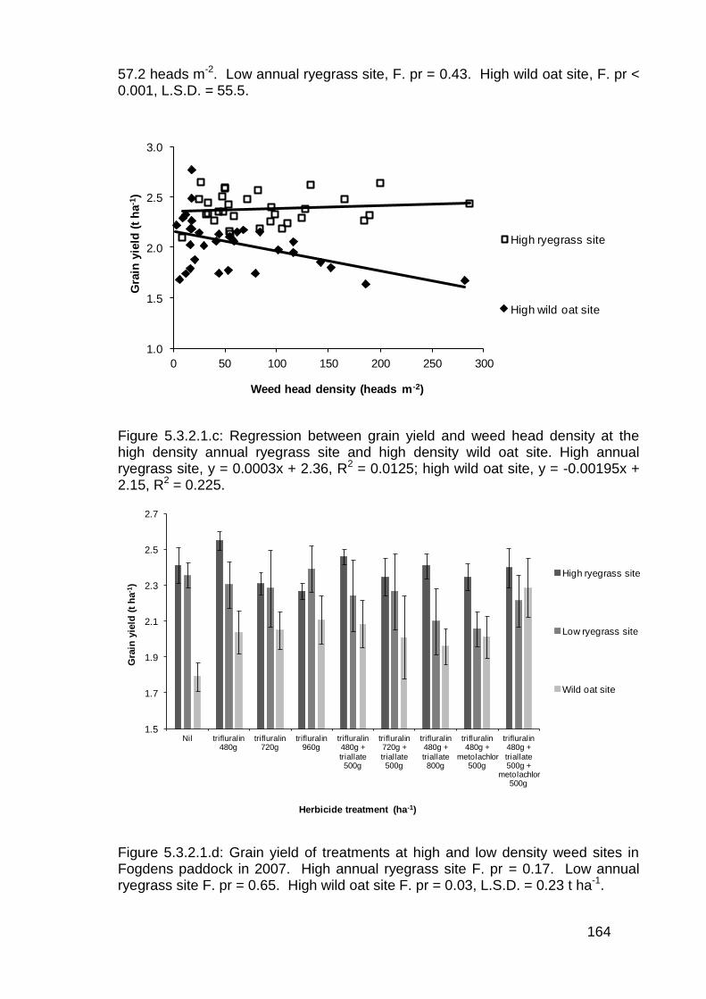
164

57.2 heads m-2. Low annual ryegrass site, F. pr = 0.43. High wild oat site, F. pr < 0.001, L.S.D. = 55.5.

1.0

1.5

2.0

2.5

3.0

0 50 100 150 200 250 300

Gra

in y

ield

(t

ha

-1)

Weed head density (heads m-2)

High ryegrass site

High wild oat site

Figure 5.3.2.1.c: Regression between grain yield and weed head density at the high density annual ryegrass site and high density wild oat site. High annual ryegrass site, y = 0.0003x + 2.36, R2 = 0.0125; high wild oat site, y = -0.00195x + 2.15, R2 = 0.225.

1.5

1.7

1.9

2.1

2.3

2.5

2.7

Nil trifluralin 480g

trifluralin 720g

trifluralin 960g

trifluralin 480g +

triallate 500g

trifluralin 720g +

triallate 500g

trifluralin 480g +

triallate 800g

trifluralin 480g +

metolachlor 500g

trifluralin 480g +

triallate 500g +

metolachlor 500g

Gra

in y

ield

(t

ha

-1)

Herbicide treatment (ha-1)

High ryegrass site

Low ryegrass site

Wild oat site

Figure 5.3.2.1.d: Grain yield of treatments at high and low density weed sites in Fogdens paddock in 2007. High annual ryegrass site F. pr = 0.17. Low annual ryegrass site F. pr = 0.65. High wild oat site F. pr = 0.03, L.S.D. = 0.23 t ha-1.

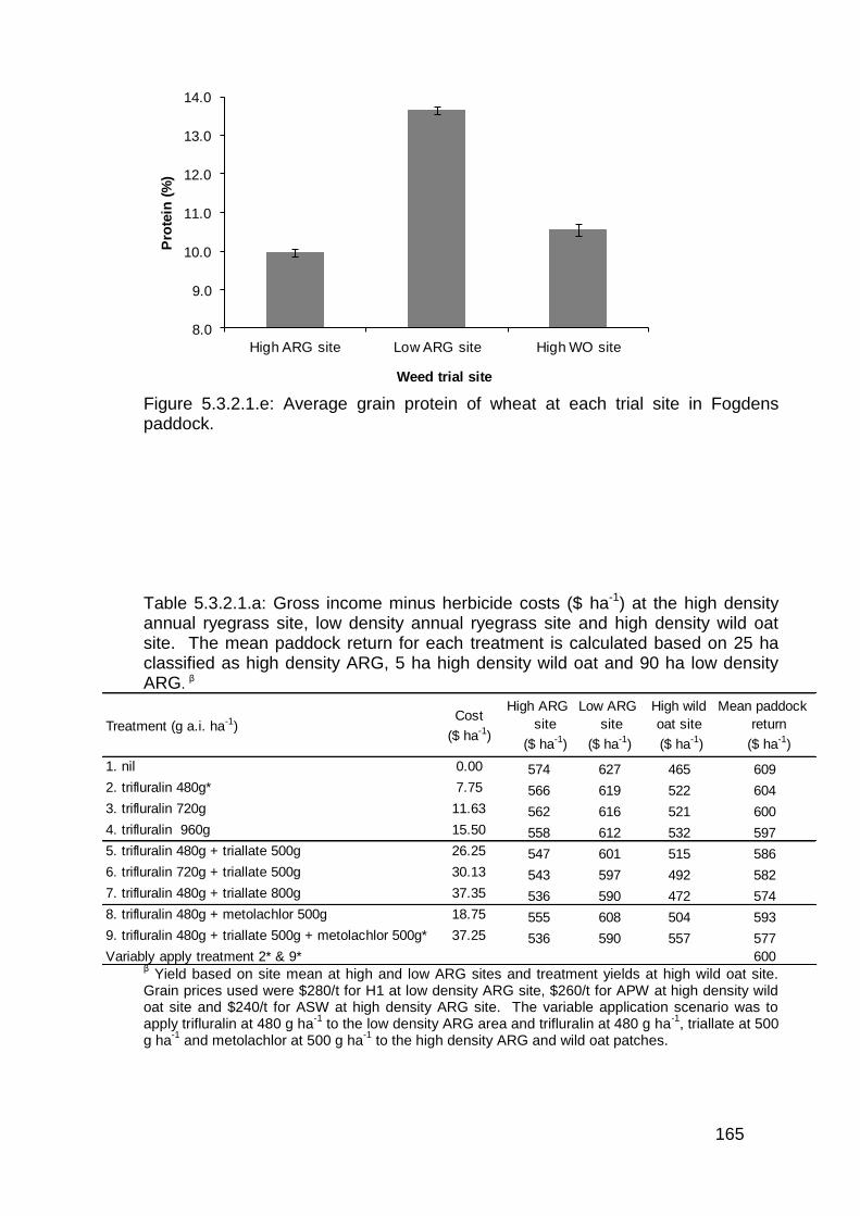
165

8.0

9.0

10.0

11.0

12.0

13.0

14.0

High ARG site Low ARG site High WO site

Pro

tein

(%

)

Weed trial site

Figure 5.3.2.1.e: Average grain protein of wheat at each trial site in Fogdens paddock. Table 5.3.2.1.a: Gross income minus herbicide costs ($ ha-1) at the high density annual ryegrass site, low density annual ryegrass site and high density wild oat site. The mean paddock return for each treatment is calculated based on 25 ha classified as high density ARG, 5 ha high density wild oat and 90 ha low density ARG.

β

Treatment (g a.i. ha-1) Cost

($ ha-1)

High ARG

site

($ ha-1)

Low ARG

site

($ ha-1)

High wild

oat site

($ ha-1)

Mean paddock

return

($ ha-1)

1. nil 0.00 574 627 465 609

2. trifluralin 480g* 7.75 566 619 522 604

3. trifluralin 720g 11.63 562 616 521 600

4. trifluralin 960g 15.50 558 612 532 597

5. trifluralin 480g + triallate 500g 26.25 547 601 515 586

6. trifluralin 720g + triallate 500g 30.13 543 597 492 582

7. trifluralin 480g + triallate 800g 37.35 536 590 472 574

8. trifluralin 480g + metolachlor 500g 18.75 555 608 504 593

9. trifluralin 480g + triallate 500g + metolachlor 500g* 37.25 536 590 557 577

Variably apply treatment 2* & 9* 600 β Yield based on site mean at high and low ARG sites and treatment yields at high wild oat site.

Grain prices used were $280/t for H1 at low density ARG site, $260/t for APW at high density wild oat site and $240/t for ASW at high density ARG site. The variable application scenario was to apply trifluralin at 480 g ha

-1 to the low density ARG area and trifluralin at 480 g ha

-1, triallate at 500

g ha-1

and metolachlor at 500 g ha-1

to the high density ARG and wild oat patches.

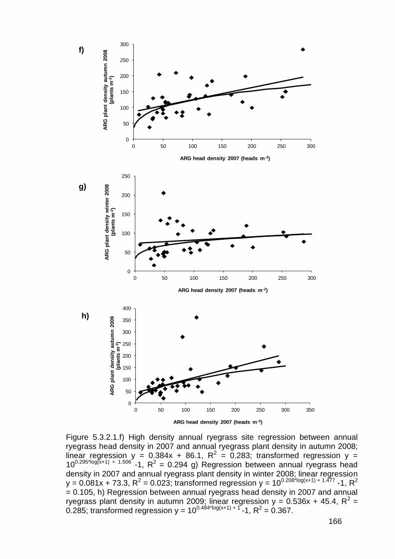
166

0

50

100

150

200

250

300

0 50 100 150 200 250 300

AR

G p

lan

t d

en

sit

y a

utu

mn

2008

(pla

nts

m-2

)

ARG head density 2007 (heads m-2)

0

50

100

150

200

250

0 50 100 150 200 250 300

AR

G p

lan

t d

en

sit

y w

inte

r 2008

(pla

nts

m-2

)

ARG head density 2007 (heads m-2)

0

50

100

150

200

250

300

350

400

0 50 100 150 200 250 300 350

AR

G p

lan

t d

en

sit

y a

utu

mn

2009

(p

lan

ts m

-2)

ARG head density 2007 (heads m-2)

Figure 5.3.2.1.f) High density annual ryegrass site regression between annual ryegrass head density in 2007 and annual ryegrass plant density in autumn 2008; linear regression y = 0.384x + 86.1, R2 = 0.283; transformed regression y = 100.295*log(x+1) + 1.506 -1, R2 = 0.294 g) Regression between annual ryegrass head density in 2007 and annual ryegrass plant density in winter 2008; linear regression y = 0.081x + 73.3, R2 = 0.023; transformed regression y = 100.208*log(x+1) + 1.477 -1, R2 = 0.105, h) Regression between annual ryegrass head density in 2007 and annual ryegrass plant density in autumn 2009; linear regression y = 0.536x + 45.4, R2 = 0.285; transformed regression y = 100.484*log(x+1) + 1 -1, R2 = 0.367.

f)

h)

g)

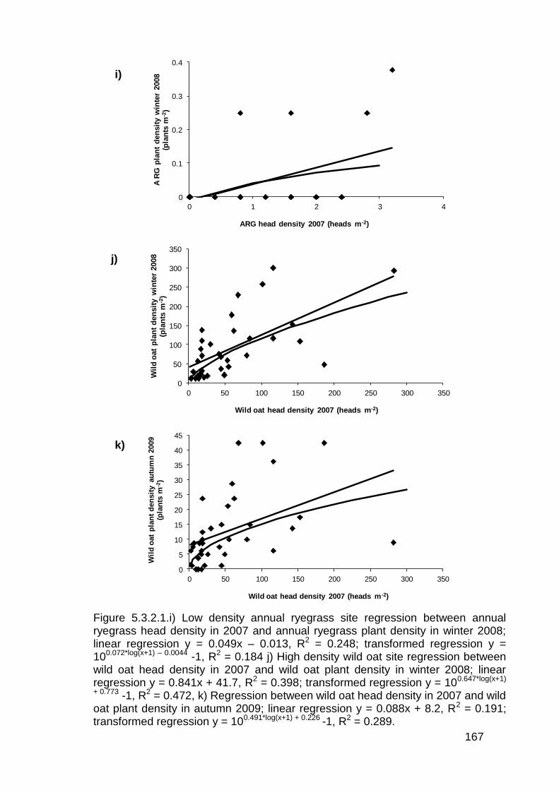
167

0

0.1

0.2

0.3

0.4

0 1 2 3 4

A R

G p

lan

t d

en

sit

y w

inte

r 2008

(p

lan

ts m

-2)

ARG head density 2007 (heads m-2)

0

50

100

150

200

250

300

350

0 50 100 150 200 250 300 350

Wil

d o

at

pla

nt

den

sit

y w

inte

r 2008

(pla

nts

m-2

)

Wild oat head density 2007 (heads m-2)

0

5

10

15

20

25

30

35

40

45

0 50 100 150 200 250 300 350

Wil

d o

at

pla

nt

den

sit

y a

utu

mn

2009

(pla

nts

m-2

)

Wild oat head density 2007 (heads m-2)

Figure 5.3.2.1.i) Low density annual ryegrass site regression between annual ryegrass head density in 2007 and annual ryegrass plant density in winter 2008; linear regression y = 0.049x – 0.013, R2 = 0.248; transformed regression y = 100.072*log(x+1) – 0.0044 -1, R2 = 0.184 j) High density wild oat site regression between wild oat head density in 2007 and wild oat plant density in winter 2008; linear regression y = 0.841x + 41.7, R2 = 0.398; transformed regression y = 100.647*log(x+1)

+ 0.773 -1, R2 = 0.472, k) Regression between wild oat head density in 2007 and wild oat plant density in autumn 2009; linear regression y = 0.088x + 8.2, R2 = 0.191; transformed regression y = 100.491*log(x+1) + 0.226 -1, R2 = 0.289.

i)

k)

j)

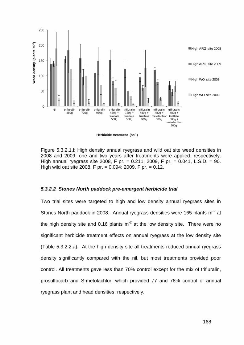
168

0

50

100

150

200

250

Nil trifluralin 480g

trifluralin 720g

trifluralin 960g

trifluralin 480g +

triallate 500g

trifluralin 720g +

triallate 500g

trifluralin 480g +

triallate 800g

trifluralin 480g +

metolachlor 500g

trifluralin 480g +

triallate 500g +

metolachlor 500g

Weed

den

sit

y (

pla

nts

m-2

)

Herbicide treatment (ha-1)

High ARG site 2008

High ARG site 2009

High WO site 2008

High WO site 2009

Figure 5.3.2.1.l: High density annual ryegrass and wild oat site weed densities in 2008 and 2009, one and two years after treatments were applied, respectively. High annual ryegrass site 2008, F pr. = 0.211; 2009, F pr. = 0.041, L.S.D. = 90. High wild oat site 2008, F pr. = 0.094; 2009, F pr. = 0.12.

5.3.2.2 Stones North paddock pre-emergent herbicide trial

Two trial sites were targeted to high and low density annual ryegrass sites in

Stones North paddock in 2008. Annual ryegrass densities were 165 plants m-2 at

the high density site and 0.16 plants m-2 at the low density site. There were no

significant herbicide treatment effects on annual ryegrass at the low density site

(Table 5.3.2.2.a). At the high density site all treatments reduced annual ryegrass

density significantly compared with the nil, but most treatments provided poor

control. All treatments gave less than 70% control except for the mix of trifluralin,

prosulfocarb and S-metolachlor, which provided 77 and 78% control of annual

ryegrass plant and head densities, respectively.

169

There was a strong negative linear relationship between annual ryegrass head

density and wheat yield at the high density site where yield declined by 2 kg ha-1

with each additional annual ryegrass head m-2 (Figure 5.3.2.2.a). This resulted in

a significant treatment effect on yield at the high density site where the trifluralin,

prosulfocarb and S-metolachlor mixture yielded significantly more than all other

treatments except the prosulfocarb and S-metolachlor mixture (Figure 5.3.2.2.b).

There were no significant treatment effects at the low density annual ryegrass site.

At the high density annual ryegrass site there was a positive correlation between

annual ryegrass head density in 2008 and annual ryegrass plant density in autumn

2009 (Figure 5.3.2.2.c). There is no such relationship at the low density site

(Figure 5.3.2.2.d). The herbicide mixture of trifluralin, prosulfocarb and S-

metolachlor resulted in the lowest annual ryegrass density in autumn 2009 at the

high density site, with 1215 plants m-2 (Figure 5.3.2.2.e), and was the only

herbicide treatment that was significantly lower than the nil with 3385 plants m-2.

Table 5.3.2.2.a: Herbicide treatment effects on annual ryegrass plant and head density at high and low density sites in Stones North paddock 26 and 196 days after application.

plants m-2 % control heads m

-2 % control plants m-2

heads m-2

nil 165 660 0.16 3.69

trifluralin 480 g 107 35 457 31 0.06 0.09

trifluralin 960 g 97 41 354 46 0.13 1.70

triallate 800 g 95 43 309 53 0.06 1.89

s-metolachlor 480 g 126 23 494 25 0.22 1.42

prosulfocarb 2000g + s-metolachlor 300g 76 54 208 69 0.06 0.47

trifluralin 480g + triallate 800g 75 54 267 60 0.13 0.00

trifluralin 480g + s-metolachlor 480g 114 31 531 20 0.00 0.66

trifluralin 480g + prosulfocarb 2000g + s-

metolachlor 300g38 77 143 78 0.28 0.09

trifluralin 480g + triallate 500g + s-

metolachlor 336g63 62 323 51 0.06 0.28

trifluralin 480g + triallate 800g + s-

metolachlor 480g80 51 308 53 0.38 0.66

F pr. <0.001 <0.001 <0.001 <0.001 0.507 0.160

L.S.D. 36 19 127 18 ns ns

Treatment (g a.i. ha-1

)

High ryegrass site Low ryegrass site

ns = not significant

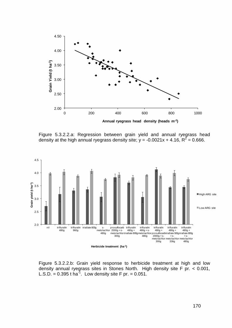
170

2.00

2.50

3.00

3.50

4.00

4.50

0 200 400 600 800 1000

Gra

in Y

ield

(t

ha

-1)

Annual ryegrass head density (heads m-2)

Figure 5.3.2.2.a: Regression between grain yield and annual ryegrass head density at the high annual ryegrass density site; y = -0.0021x + 4.16, R2 = 0.666.

2.0

2.5

3.0

3.5

4.0

4.5

nil trifluralin 480g

trifluralin 960g

triallate 800g s-metolachlor

480g

prosulfocarb 2000g + s-

metolachlor 300g

trifluralin 480g +

triallate 800g

trifluralin 480g + s-

metolachlor 480g

trifluralin 480g +

prosulfocarb 2000g + s-

metolachlor 300g

trifluralin 480g +

triallate 500g + s-

metolachlor 336g

trifluralin 480g +

triallate 800g + s-

metolachlor 480g

Gra

in y

ield

(t

ha

-1)

Herbicide treatment (ha-1)

High ARG site

Low ARG site

Figure 5.3.2.2.b: Grain yield response to herbicide treatment at high and low density annual ryegrass sites in Stones North. High density site F pr. < 0.001, L.S.D. = 0.395 t ha-1. Low density site F pr. = 0.051.

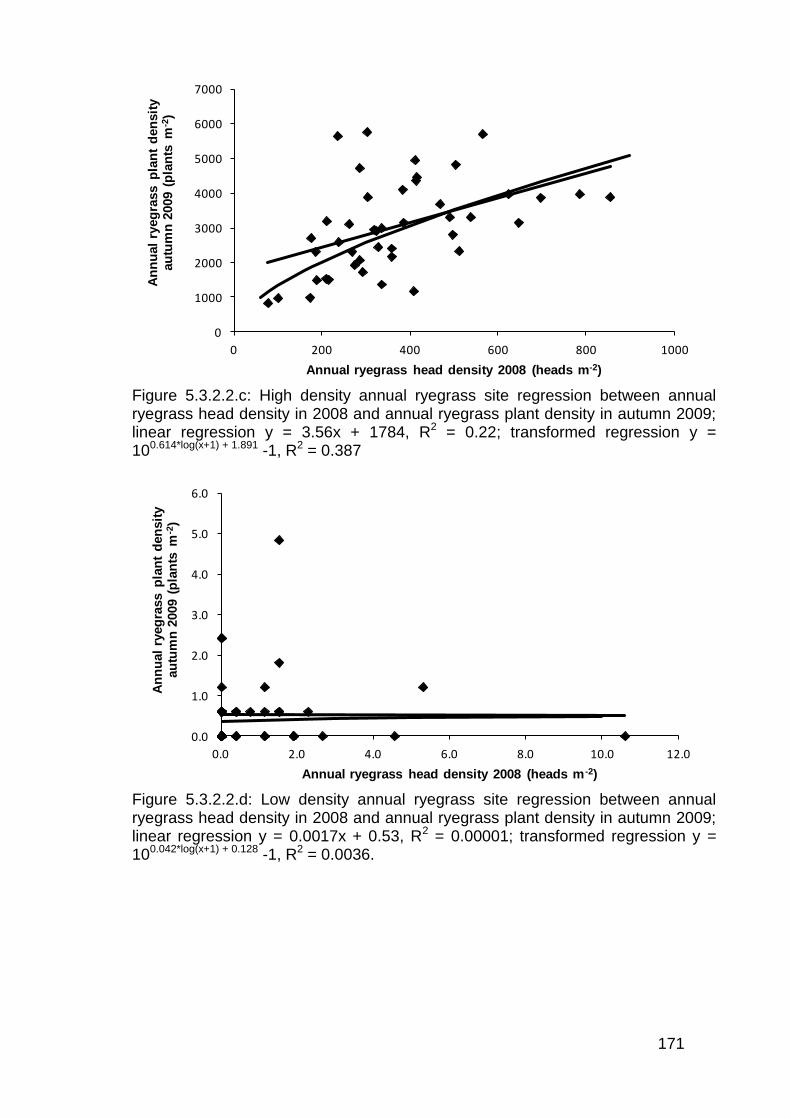
171

0

1000

2000

3000

4000

5000

6000

7000

0 200 400 600 800 1000

An

nu

al

ryeg

rass p

lan

t d

en

sit

y

au

tum

n 2

009 (

pla

nts

m-2

)

Annual ryegrass head density 2008 (heads m-2)

Figure 5.3.2.2.c: High density annual ryegrass site regression between annual ryegrass head density in 2008 and annual ryegrass plant density in autumn 2009; linear regression y = 3.56x + 1784, R2 = 0.22; transformed regression y = 100.614*log(x+1) + 1.891 -1, R2 = 0.387

0.0

1.0

2.0

3.0

4.0

5.0

6.0

0.0 2.0 4.0 6.0 8.0 10.0 12.0

An

nu

al

ryeg

rass p

lan

t d

en

sit

y

au

tum

n 2

009 (

pla

nts

m-2

)

Annual ryegrass head density 2008 (heads m -2)

Figure 5.3.2.2.d: Low density annual ryegrass site regression between annual ryegrass head density in 2008 and annual ryegrass plant density in autumn 2009; linear regression y = 0.0017x + 0.53, R2 = 0.00001; transformed regression y = 100.042*log(x+1) + 0.128 -1, R2 = 0.0036.

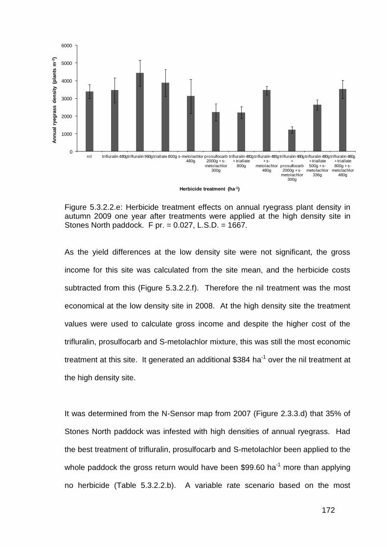
172

0

1000

2000

3000

4000

5000

6000

nil trifluralin 480gtrifluralin 960gtriallate 800g s-metolachlor 480g

prosulfocarb 2000g + s-

metolachlor 300g

trifluralin 480g + triallate

800g

trifluralin 480g + s-

metolachlor 480g

trifluralin 480g +

prosulfocarb 2000g + s-

metolachlor 300g

trifluralin 480g + triallate

500g + s-metolachlor

336g

trifluralin 480g + triallate

800g + s-metolachlor

480g

An

nu

al

ryeg

rass d

en

sit

y (

pla

nts

m-2

)

Herbicide treatment (ha-1)

Figure 5.3.2.2.e: Herbicide treatment effects on annual ryegrass plant density in autumn 2009 one year after treatments were applied at the high density site in Stones North paddock. F pr. = 0.027, L.S.D. = 1667.

As the yield differences at the low density site were not significant, the gross

income for this site was calculated from the site mean, and the herbicide costs

subtracted from this (Figure 5.3.2.2.f). Therefore the nil treatment was the most

economical at the low density site in 2008. At the high density site the treatment

values were used to calculate gross income and despite the higher cost of the

trifluralin, prosulfocarb and S-metolachlor mixture, this was still the most economic

treatment at this site. It generated an additional $384 ha-1 over the nil treatment at

the high density site.

It was determined from the N-Sensor map from 2007 (Figure 2.3.3.d) that 35% of

Stones North paddock was infested with high densities of annual ryegrass. Had

the best treatment of trifluralin, prosulfocarb and S-metolachlor been applied to the

whole paddock the gross return would have been $99.60 ha-1 more than applying

no herbicide (Table 5.3.2.2.b). A variable rate scenario based on the most

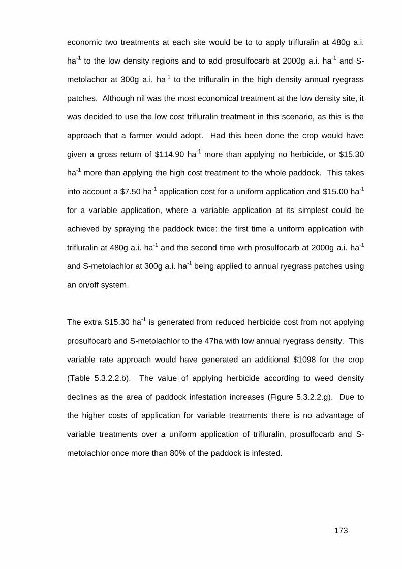
173

economic two treatments at each site would be to to apply trifluralin at 480g a.i.

ha-1 to the low density regions and to add prosulfocarb at 2000g a.i. ha-1 and S-

metolachor at 300g a.i. ha-1 to the trifluralin in the high density annual ryegrass

patches. Although nil was the most economical treatment at the low density site, it

was decided to use the low cost trifluralin treatment in this scenario, as this is the

approach that a farmer would adopt. Had this been done the crop would have

given a gross return of $114.90 ha-1 more than applying no herbicide, or $15.30

ha-1 more than applying the high cost treatment to the whole paddock. This takes

into account a $7.50 ha-1 application cost for a uniform application and $15.00 ha-1

for a variable application, where a variable application at its simplest could be

achieved by spraying the paddock twice: the first time a uniform application with

trifluralin at 480g a.i. ha-1 and the second time with prosulfocarb at 2000g a.i. ha-1

and S-metolachlor at 300g a.i. ha-1 being applied to annual ryegrass patches using

an on/off system.

The extra $15.30 ha-1 is generated from reduced herbicide cost from not applying

prosulfocarb and S-metolachlor to the 47ha with low annual ryegrass density. This

variable rate approach would have generated an additional $1098 for the crop

(Table 5.3.2.2.b). The value of applying herbicide according to weed density

declines as the area of paddock infestation increases (Figure 5.3.2.2.g). Due to

the higher costs of application for variable treatments there is no advantage of

variable treatments over a uniform application of trifluralin, prosulfocarb and S-

metolachlor once more than 80% of the paddock is infested.

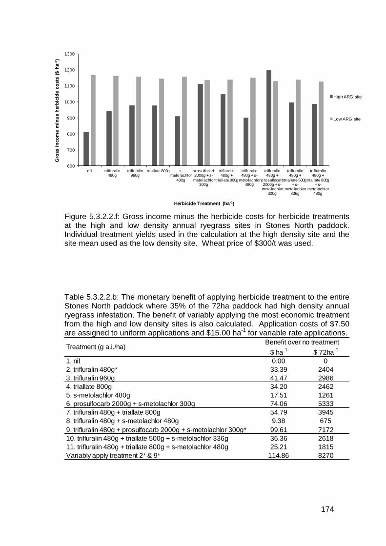
174

600

700

800

900

1000

1100

1200

1300

nil trifluralin 480g

trifluralin 960g

triallate 800g s-metolachlor

480g

prosulfocarb 2000g + s-

metolachlor 300g

trifluralin 480g +

triallate 800g

trifluralin 480g + s-

metolachlor 480g

trifluralin 480g +

prosulfocarb 2000g + s-metolachlor

300g

trifluralin 480g +

triallate 500g + s-

metolachlor 336g

trifluralin 480g +

triallate 800g + s-

metolachlor 480g

Gro

ss I

nco

me m

inu

s h

erb

icid

e c

osts

($ h

a-1

)

Herbicide Treatment (ha-1)

High ARG site

Low ARG site

Figure 5.3.2.2.f: Gross income minus the herbicide costs for herbicide treatments at the high and low density annual ryegrass sites in Stones North paddock. Individual treatment yields used in the calculation at the high density site and the site mean used as the low density site. Wheat price of $300/t was used. Table 5.3.2.2.b: The monetary benefit of applying herbicide treatment to the entire Stones North paddock where 35% of the 72ha paddock had high density annual ryegrass infestation. The benefit of variably applying the most economic treatment from the high and low density sites is also calculated. Application costs of $7.50 are assigned to uniform applications and $15.00 ha-1 for variable rate applications.

$ ha-1

$ 72ha-1

1. nil 0.00 0

2. trifluralin 480g* 33.39 2404

3. trifluralin 960g 41.47 2986

4. triallate 800g 34.20 2462

5. s-metolachlor 480g 17.51 1261

6. prosulfocarb 2000g + s-metolachlor 300g 74.06 5333

7. trifluralin 480g + triallate 800g 54.79 3945

8. trifluralin 480g + s-metolachlor 480g 9.38 675

9. trifluralin 480g + prosulfocarb 2000g + s-metolachlor 300g* 99.61 7172

10. trifluralin 480g + triallate 500g + s-metolachlor 336g 36.36 2618

11. trifluralin 480g + triallate 800g + s-metolachlor 480g 25.21 1815

Variably apply treatment 2* & 9* 114.86 8270

Benefit over no treatmentTreatment (g a.i./ha)

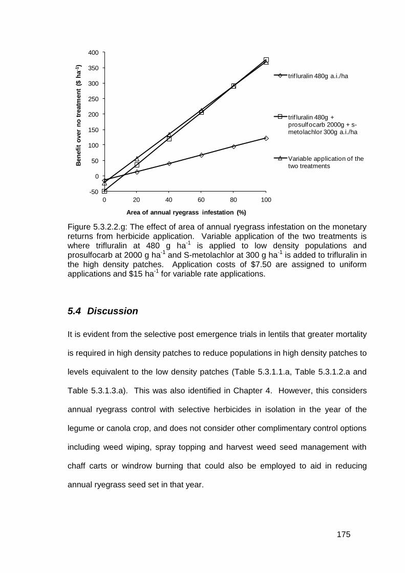
175

-50

0

50

100

150

200

250

300

350

400

0 20 40 60 80 100

Ben

efi

t o

ver

no

tre

atm

en

t ($

ha

-1)

Area of annual ryegrass infestation (%)

trif luralin 480g a.i./ha

trif luralin 480g + prosulfocarb 2000g + s-metolachlor 300g a.i./ha

Variable application of the two treatments

Figure 5.3.2.2.g: The effect of area of annual ryegrass infestation on the monetary returns from herbicide application. Variable application of the two treatments is where trifluralin at 480 g ha-1 is applied to low density populations and prosulfocarb at 2000 g ha-1 and S-metolachlor at 300 g ha-1 is added to trifluralin in the high density patches. Application costs of $7.50 are assigned to uniform applications and $15 ha-1 for variable rate applications.

5.4 Discussion

It is evident from the selective post emergence trials in lentils that greater mortality

is required in high density patches to reduce populations in high density patches to

levels equivalent to the low density patches (Table 5.3.1.1.a, Table 5.3.1.2.a and

Table 5.3.1.3.a). This was also identified in Chapter 4. However, this considers

annual ryegrass control with selective herbicides in isolation in the year of the

legume or canola crop, and does not consider other complimentary control options

including weed wiping, spray topping and harvest weed seed management with

chaff carts or windrow burning that could also be employed to aid in reducing

annual ryegrass seed set in that year.

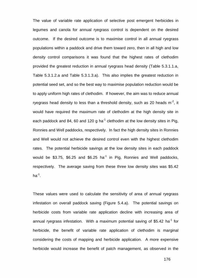
176

The value of variable rate application of selective post emergent herbicides in

legumes and canola for annual ryegrass control is dependent on the desired

outcome. If the desired outcome is to maximise control in all annual ryegrass

populations within a paddock and drive them toward zero, then in all high and low

density control comparisons it was found that the highest rates of clethodim

provided the greatest reduction in annual ryegrass head density (Table 5.3.1.1.a,

Table 5.3.1.2.a and Table 5.3.1.3.a). This also implies the greatest reduction in

potential seed set, and so the best way to maximise population reduction would be

to apply uniform high rates of clethodim. If however, the aim was to reduce annual

ryegrass head density to less than a threshold density, such as 20 heads m-2, it

would have required the maximum rate of clethodim at the high density site in

each paddock and 84, 60 and 120 g ha-1 clethodim at the low density sites in Pig,

Ronnies and Well paddocks, respectively. In fact the high density sites in Ronnies

and Well would not achieve the desired control even with the highest clethodim

rates. The potential herbicide savings at the low density sites in each paddock

would be $3.75, $6.25 and $6.25 ha-1 in Pig, Ronnies and Well paddocks,

respectively. The average saving from these three low density sites was $5.42

ha-1.

These values were used to calculate the sensitivity of area of annual ryegrass

infestation on overall paddock saving (Figure 5.4.a). The potential savings on

herbicide costs from variable rate application decline with increasing area of

annual ryegrass infestation. With a maximum potential saving of $5.42 ha-1 for

herbicide, the benefit of variable rate application of clethodim is marginal

considering the costs of mapping and herbicide application. A more expensive

herbicide would increase the benefit of patch management, as observed in the

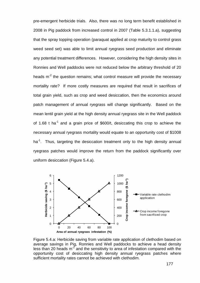
177

pre-emergent herbicide trials. Also, there was no long term benefit established in

2008 in Pig paddock from increased control in 2007 (Table 5.3.1.1.a), suggesting

that the spray topping operation (paraquat applied at crop maturity to control grass

weed seed set) was able to limit annual ryegrass seed production and eliminate

any potential treatment differences. However, considering the high density sites in

Ronnies and Well paddocks were not reduced below the arbitrary threshold of 20

heads m-2 the question remains; what control measure will provide the necessary

mortality rate? If more costly measures are required that result in sacrifices of

total grain yield, such as crop and weed desiccation, then the economics around

patch management of annual ryegrass will change significantly. Based on the

mean lentil grain yield at the high density annual ryegrass site in the Well paddock

of 1.68 t ha-1 and a grain price of $600/t, desiccating this crop to achieve the

necessary annual ryegrass mortality would equate to an opportunity cost of $1008

ha-1. Thus, targeting the desiccation treatment only to the high density annual

ryegrass patches would improve the return from the paddock significantly over

uniform desiccation (Figure 5.4.a).

0

200

400

600

800

1000

1200

0

1

2

3

4

5

6

0 20 40 60 80 100

Cro

p i

nco

me f

ore

go

ne (

$ h

a-1

)

Herb

icid

e s

avin

g (

$ h

a-1

)

Area of annual ryegrass infestation (%)

Variable rate clethodim application

Crop income foregone f rom sacrif iced crop

Figure 5.4.a: Herbicide saving from variable rate application of clethodim based on average savings in Pig, Ronnies and Well paddocks to achieve a head density less than 20 heads m-2 and the sensitivity to area of infestation compared with the opportunity cost of desiccating high density annual ryegrass patches where sufficient mortality rates cannot be achieved with clethodim.

178

The value of site specific management of weeds cannot exceed the value of the

herbicides used, unless the herbicide has a phytotoxic crop effect that reduces

crop yield, either in the year of application or in subsequent years. No trials in this

study suffered any measurable yield loss from herbicide phytotoxicity. There were

no significant yield differences in response to herbicide treatment at the low

density annual ryegrass sites in Well, Fogdens and Stones North paddock (Table

5.3.1.3.a, Figure 5.3.2.1.d and Figure 5.3.2.2.b), where the herbicide effect could

be observed in the absence of weed competition. Therefore, site specific weed

management is only likely to be worthwhile where more expensive herbicides are

considered, and the more expensive pre-emergence herbicides used for annual

ryegrass control in cereals fit this criteria.

A yield response to reduced weed density is necessary for herbicide application to

be economic in the year the herbicide is applied. No yield response was observed

at the high density annual ryegrass site in Fogdens paddock, despite several

treatments significantly reducing annual ryegrass density. Despite a yield

response at the high density wild oat site, a blanket application of the most

efficacious treatment of trifluralin, triallate and metolachlor would have reduced

returns by $31.90 ha-1 compared with doing nothing given the areas of infestation

in this paddock. Applying a variable rate application where trifluralin at 480 g a.i.

ha-1 is applied to the entire paddock and triallate at 500 g a.i. ha-1 and metolachlor

at 500 g a.i. ha-1 is applied to the high density weed patches would have reduced

returns by $9.80 ha-1, compared with doing nothing. While the application of

variable rate herbicide would have reduced returns compared with doing nothing, it

has reduced the risk involved with herbicide application and reduced the losses by

179

$22.10 ha-1 that the farmer would have incurred had the entire field been sprayed

with the high cost treatment.

In Stones North paddock there was a $15.30 ha-1 increase in gross margin by

applying prosulfocarb and S-metolachlor only to where the annual ryegrass

patches were in 35% of that paddock. The saving increases as area of infestation

declines. Only 5.6% of the paddock needed to be infested before the benefit of

variable rate application was better than not treating at all, i.e. the yield gain from

5.6% of the paddock infested with high densities of annual ryegrass paid for the

cost of application ($15.00 ha-1), the cost of the herbicide mix ($42.80 ha-1) to treat

the high density patches and the cost of the trifluralin ($7.80 ha-1) to treat 94.4% of

the paddock with low annual ryegrass densities where no yield gain was observed

from herbicide application.

The application cost of $15.00 ha-1 may be an overestimate, particularly when only

small areas of the paddock are classified as high density infestations. The $15.00

ha-1 assumes that the sprayer must travel over all parts of the field twice to apply

the variable treatment. However, depending on the spatial distribution of the

patches, the sprayer may be able to spray just the patches and eliminate the need

to travel over all of the low density regions of the paddock the second time when

applying the prosulfocarb and S-metolachlor. Therefore, the economic benefit may

be even greater when only small areas are infested. By comparison, if the

decision was limited to treating the whole field with the $42.80 ha-1 treatment of

trifluralin, prosulfocarb and S-metolachlor with an application cost of $7.50 ha-1 or

not treating at all, then 11.6% of the paddock would need to be infested before it

180

would pay for itself. Therefore, it is more economic to treat annual ryegrass

infestations in small patches before the patches become large.

The economic discussion above only considers the effect of the herbicide in the

year of application, and does not consider the longer term effects of weed control.

It was demonstrated at the high density annual ryegrass sites in both Stones North

and Fogdens paddocks that there was a positive correlation between annual

ryegrass control in one year and annual ryegrass population reduction in

subsequent years (Figure 5.3.2.1.e-g and Figure 5.3.2.2.c). The most efficacious

treatments in the year of application at the high density annual ryegrass sites had

significantly lower annual ryegrass densities in subsequent seasons (Figure

5.3.2.1.l and Figure 5.3.2.2.e). However, despite lower annual ryegrass densities

resulting from more efficacious treatments at high density sites, the annual

ryegrass densities remain significantly higher than the low density sites and at

densities where significant yield reductions would be expected. They also persist

for several years. For example, in Fogdens paddock at the high density annual

ryegrass site, close to 100% control was achieved in the lentils in 2006. In 2007

the treatments set seed and then in 2008 the trial site was desiccated to prevent

seed set. Despite two of three years having near 100% control at the site, the

annual ryegrass density in the most efficacious treatment in 2009 was 46 plants

m-2. This highlights the need for ongoing vigilance on high density patches to

drive numbers down and the necessity to control successive cohorts and

successive generations if high density patches are to be eliminated. It also

reinforces the findings of Chapters 3 and 4 with regard to persistence of high

density patches and the need for control of successive cohorts and generations.

181

A concern of site specific weed management is that treatment of low density weed

areas with lower efficacy herbicides will allow weeds to survive and set seed and

result in a low density population becoming a high density population within the

space of a few seasons (Lutman and Miller 2007). No evidence was observed to

support this theory in this study. Firstly, there was evidence indicating that all

herbicide treatments provided annual ryegrass control at low density sites, but

there were no significant differences between the treatments. However, the same

treatments were found to be significantly different at high density sites (Figure

5.3.2.1.a, Figure 5.3.2.1.b and Table 5.3.2.2.a). Secondly, no relationships could

be established between annual ryegrass control at low density sites and annual

ryegrass density in the following season (Figure 5.3.2.1.h and Figure 5.3.2.2.f).

Annual ryegrass is widely adapted to a wide range of growing conditions; however

anecdotal evidence in this study suggests that high density annual ryegrass

patches occur in locations where crop growth is less vigorous. The causes of

lower crop vigour can be varied, but may include salinity, boron toxicity, nutrient

deficiency, water logging, non-wetting soil, sodicity and acidity (Adcock et al.

2007). This is an observation supported by a recent study of Dr J Heap (SARDI,

pers comm.). This suggests that reduced crop competition enables annual

ryegrass to proliferate and set seed more freely. Conversely, it also suggests that

soils that support vigorous crop growth will have low annual ryegrass densities due

to higher crop competition (Medd et al. 1985). The findings of this study also

suggest that cheaper herbicide options, with potentially lower efficacy, can

maintain low annual ryegrass densities at these sites, and higher crop competition

is an important factor contributing to this. It also suggests that increasing crop

competition could be a useful tool in a long term strategy to eliminate high density

182

annual ryegrass patches, in combination with other control measures such as

herbicides. Increased competition could be targeted to annual ryegrass patches

by increasing crop seeding rates.

It was observed in Fogdens paddock that the sites of high weed density had lower

grain protein (Figure 5.3.2.1.e). Possible explanations for this include the

competition for nitrogen between the wheat crop and weeds. In addition, there

may have been less N fixation in the previous lentil crop at those sites due to the

weeds competition with lentils reducing resources for N fixation.

Weed species misclassification in patches can potentially lead to application of the

wrong herbicide to a weed patch. In Fogdens paddock the N-Sensor map had

identified patches of annual ryegrass and wild oats, but did not differentiate

between them. In this example, a herbicide control measure was available that

was efficacious on both weed species, in fact a greater economic return was

achieved from targeting herbicide to the non-target species of wild oats than

annual ryegrass. Therefore, differentiating different weed species in an application

map will be of more or less importance depending on the weed species involved.

It is important when using weed mapping systems that do not discriminate weed

species that appropriate scouting is done in conjunction with the mapping process

so that the weed species present are known. If appropriate control options that

control both species are available it will be important that these are chosen in

preference to options that control only one of the species.

183

6 Conclusions

6.1 Mapping Lolium rigidum Patches Using Spectral Reflectance

Sensors

Annual ryegrass detection and mapping is the first step in the successful

implementation of site specific management. Findings from this study indicate that

there are a range of technologies that are potentially useful for detecting annual

ryegrass patches within a growing crop. However, their limitations need to be

recognised and accounted for. The sensors utilised in this study all detect weed

patches based on the increase in photosynthetic active biomass that weeds

contribute over and above what the crop produces and do not discriminate plant

species. Thus, this method of detection will always need to be accompanied by

field observation to ground truth the maps and determine what is the cause of the

variability that the sensors measure. Misclassification of weed species can lead to

inappropriate herbicide applications. However, as demonstrated in this study,

control measures may exist that can be targeted to two or more species at the

same time, so the misclassification maybe inconsequential or even beneficial in

some cases (Chapter 5).

Time of mapping is important. Mapping should be delayed so that the weeds can

establish and grow to a size that can be detected by the sensor, but not too long

such that variability in weed density is confounded by variability in crop growth.

Crop variability is induced at earlier growth stages in paddocks with highly variable

soil types. In this study the best timings were at 9-12 node stage for lentils and 6-

12 node stage for peas when the annual ryegrass was between 1-2 leaf stage and

mid tillering (Figure 2.3.1.4.a-b). This timing corresponds with the period when

184

post emergence applications of clethodim and other grass selective herbicides

would be made, so offers the opportunity to combine the operations of real-time

mapping and spraying to save on costs.

Digital imagery from a standard 5 megapixel RGB digital camera was as good,

and in many cases better, than the alternative sensing platforms for detecting

annual ryegrass (Figure 2.3.1.6.a-b). There is merit in pursuing this technology

and in particular some more advanced technologies. Studies by Hague and Tillett

(2006) in the UK demonstrate the potential for weed detection where the crop rows

can be eliminated from the detection process so that only variability in weed

density is observed. The ‘widely spaced cereals’ that they conducted their studies

in are consistent with the crop row spacings used in Australian cropping systems.

This would eliminate the problem of crop variability confounding the detection of

weeds. Gerhards and Oebel (2006) describe a system for delineating 25

individual weed species from four different crop types and this too should be

investigated in an Australian environment. This would overcome the problems of

weed misclassification.

When designing paddock mapping strategies the resolution of mapping is an

important consideration, as higher resolution mapping corresponds with higher

mapping costs. Factors that affect spatial distribution of patches and introduce

anisotropy need to be considered and accounted for, including the concentration

of weed seeds into strips when seed passes through the combine harvester

(Figure 2.3.4.c-g). Placing sensors over the concentrated strips of annual

ryegrass in the header rows will help to ensure that all high density weed patches

are identified.

185

6.2 Patch Stability in Lolium rigidum Populations

Demonstrating stability of weed patches targeted for site specific management is

important as it determines for how long a weed map will be relevant. This study

demonstrated that high density annual ryegrass locations typically remained high

over several seasons and low density locations typically remained low (Figures

3.3.1, 3.3.2, 3.3.3, 3.3.4). Locations that changed from being relatively low to high

were commonly located near a patch boundary, suggesting that patch expansion

should be accounted for if the same map is to be used over several seasons. A

buffer, in the order of 18-20m, that accounts for seed spread by combine

harvesters should be included for subsequent seasons. The fact that the patches

are relatively stable is an important finding, as it introduces the potential for SSWM

with pre-emergent herbicides in the seasons following map generation and this is

likely the best opportunity to realise an economic advantage from SSWM of annual

ryegrass.

Understanding why the annual ryegrass patches are where they are may provide

clues to their long term management. There is evidence to suggest that the

patches are most persistent where early crop growth is constrained by soil factors

such as salinity or nutrition, and this lack of crop competition provides annual

ryegrass with a competitive advantage (Gill 1996a, John Heap, pers comm.).

Strategies that counter the poorer early crop growth may improve the long term

management of these patches, for example increasing sowing rates to improve

early weed competition may be useful.

186

6.3 Post Emergent Herbicide Efficacy Dependence on Lolium

rigidum Density

It has been suggested that poorer efficacy is achieved with herbicides in high

density patches, as overlapping leaves and plants make it more difficult for all

plants to receive a lethal dose of herbicide. This was not found in this study on

annual ryegrass with the herbicides clethodim, imazapic and imazapyr. Herbicide

efficacy was found to be independent of annual ryegrass density. However, there

were more survivors in high density patches due to the higher initial population.

Seed production from these survivors is likely to help the persistence of these

patches.

6.4 Herbicide Treatment Options for Patch Management of

Lolium rigidum

Variable rate applications of selective herbicides for control of annual ryegrass in

South Australia are limited primarily to Dim herbicides in broadleaf crops and pre-

emergent herbicides in cereals (Boutsalis et al. 2012). The return from SSWM

with herbicides can’t exceed the cost of the herbicide unless the herbicide has a

phytotoxic effect on the crop that reduces yield. In this study it was found that

variable rate application of clethodim is not likely to pay, as it is a relatively low

cost herbicide. The maximum potential saving from clethodim was $5.42 ha-1 and

declines as infestation area increases. Therefore, when the cost of mapping and

application are considered the returns will only be small. However, at high density

annual ryegrass sites in Ronnies and Well paddocks the desired level of mortality

was not achieved even at the highest rates. If alternative control measures such

187

as crop and weed desiccation need to be employed that sacrifices yield, then the

economics of patch management change significantly (Figure 5.4.a).

Variable rate applications of pre-emergence herbicides in wheat were more

economically viable, as these herbicides are typically more expensive. The

herbicide savings are dependent on infestation level (Figure 5.3.2.2.d), but in

Stones North paddock where 35% of the paddock was infested variable rate

application would have generated a saving of $15.30 ha-1. Variable rate

applications also reduced the risk of low returns from using high cost herbicides

and made it more economic to treat smaller patches compared with treating the

whole paddock with a high cost treatment. No significant population increases

were identified in low density patches from using lower cost or nil treatments at

these sites.

6.5 Future Research Directions

Future research should focus on a couple of areas. The first is more precise

mapping technologies that can detect weeds at low density amongst a wider

variety of crop species than was assessed in this study. This should include

investigating systems with species identification capabilities. The second area for

future research should focus on rotational strategies for controlling annual

ryegrass patches and the economic benefits of doing so, beyond a single year of

control. This should include investigating the link between crop vigour, soil

constraints and the presence of high density annual ryegrass populations, with the

hypothesis that weed management can be improved by reducing constraints to

crop growth and increasing competition.

188

7 References

Adcock D P, McNeill A M, McDonald G K & Armstrong R D (2007). Subsoil

constraints to crop production on neutral and alkaline soils in south-eastern

Australia: a review of current knowledge and management strategies, Australian

Journal of Experimental Agriculture, 47, p 1245-1261.

Andreason C, Rudemo M & Sevestre S (1997). Assessment of weed density at an

early stage by use of image processing. Weed Research, 37, p 5-18.

Asner G P (1998). Biophysical and biochemical sources of variability in canopy

reflectance. Remote Sensing of Environment, 64, p 234-253.

Australian bureau of agricultural and resource economics (2008a). Australian

Commodities. Vol 15, no. 1, March quarter 08.1, ABARE, Canberra.

Australian bureau of agricultural and resource economics (2008b). Australian

Commodities. Vol 15, no. 3, September quarter 08.3, ABARE, Canberra.

Australian bureau of agricultural and resource economics (2008c). AGsurf.

http://www.abareconomics.com/ame/agsurf/agsurf.asp

Backes M & Plümer L (2005). Describing weed patches by shape parameters. In

Precision Agriculture ’05, Papers presented at the 5th European Conference on

Precision Agriculture, Uppsala, Sweden, p 163-168.

189

Barroso J, Fernandez-Quintanilla C, Maxwell B D & Rew L J (2004). Simulating

the effects of weed spatial pattern and resolution of mapping and spraying on

economics of site-specific management. Weed Research, 44, p 460-468.

Barroso J, Navarrete L, Sanchez Del Arco M J, Fernandez-Quintanilla C, Lutman,

P J W, Perry N H & Hull R I (2006). Dispersal of Avena Fatua and Avena Sterilis

patches by natural dissemination, soil tillage and combine harvesters. Weed

Research, 46, p 118-128.

Blanco-Moreno, J M, Chamorro, L, Masalles, R M, Recasens, J & Sans, F X

(2004). Spatial distribution of Lolium rigidum seedlings following seed dispersal by

combine harvesters. Weed Research, 44, p 375-387.

Blanco-Moreno J M, Chamorro L & Sans F X (2006). Spatial and temporal

patterns of Lolium rigidum – Avena sterilis mixed populations in a cereal field.

Weed Research, 46, p 207-218.

Blasco J, Aleixos N, Roger J M, Rabatel G & Molto E (2002). Robotic weed control

using machine vision. Biosystems Engineering, 83, p 149-157.

Blumhorst M R, Weber J B & Swain L R (1990). Efficacy of selected herbicides as

influenced by soil properties. Weed Technology, 4, p 279-283.

Borregaard T, Nielsen H, Norgaard L & Have H (2000). Crop-weed discrimination

by line imaging spectroscopy. Journal of Agricultural Engineering Research, 75, p

389-400.

190

Boutsalis P, Gill G & Preston C (2010). New mode of action herbicides to combat

herbicide resistant annual ryegrass (Lolium rigidum) in Australian cereal

production. In 17th Australasian Weeds Conference, Papers presented at the 17th

Australasian Weeds, Christchurch, New Zealand, p 278-280.

Boutsalis P, Gill G S & Preston C (2012). Incidence of herbicide resistance in rigid

ryegrass (Lolium rigidum) across south-eastern Australia. Weed Technology. 26,

in press.

Brain P & Cousens R (1990). The effect of weed distribution on predictions of yield

loss. Journal of Applied Ecology, 27, p 735-742.

Brennan LE, Robertson MJ, Dalgliesh NP & Brown S (2007). Pay-offs to zone

management in a variable climate: an example of nitrogen fertiliser on wheat.

Australian Journal of Agricultural Research, 58, p 1046-1058.

Broster J C & Pratley J E (2006). A decade of monitoring herbicide resistance in

Lolium rigidum in Australia. Australian Journal of Experimental Agriculture, 46, p

1151-1160.

Brown R B & Noble S D (2005). Site-specific weed management: sensing

requirements - what do we need to see? Weed Science, 53, p 252-258.

Burnham K P & Anderson D R (2002). Model Selection and Multimodel Inference:

A Practical Information-Theoretical Approach. 2nd ed. New York: Springer-Verlag.

191

Cardina J, Johnson G A & Sparrow D H (1997). The nature and consequence of

weed spatial distribution. Weed Science, 45, p 364-373.

Carter G A (1993). Responses of leaf spectral reflectance to plant stress.

American Journal of Botany,80, p 239-243.

Chauhan B S, Gill G S & Preston C (2006a). Influence of tillage systems on

vertical distribution, seedling recruitment and persistence of rigid ryegrass (Lolium

rigidum) seed bank. Weed Science, 54, p 669-676.

Chauhan B S, Gill G S & Preston C (2006b). Influence of environmental factors on

seed germination and seedling emergence of rigid ryegrass (Lolium rigidum).

Weed Science, 54, p 1004-1012.

Chauhan B S, Gill G S & Preston C (2007). Effect of seeding systems and

dinitroaniline herbicides on emergence and control of rigid ryegrass (Lolium

rigidum) in wheat. Weed Technology, 21, p 53-58.

Cousens R D, Wallinga J & Shaw M (2004). Are the spatial patterns of weeds

scale-invariant? Oikos, 107, p 251-264.

Keränen M, Aro E, Tyystjärvi E & Nevalainen O (2003). Automatic plant

identification with chlorophyll fluorescence fingerprinting. Precision Agriculture, 4,

p 53-67.

192

Chang J, Clay S A, Clay D E & Dalsted K (2004). Detecting weed-free and weed-

infested areas of a soybean field using near-infrared spectral data. Weed Science,

52, p 642-648.

Christensen S, Heisel T, Walter A M & Graglia E (2003). A decision algorithm for

patch spraying. Weed Research, 43, p 276-284.

Colbach N, Forcella F & Johnson G A (2000). Spatial and temporal stability of

weed populations over five years. Weed Science, 48, p 366-377.

Combellack H (1987). Weed control pursuits in Australia. Chemistry and Industry,

8, p 273-280.

Cousens R D & Woolcock J L (1997). Spatial dynamics of weeds: an overview. In:

Proceedings 1997 Brighton Crop Protection Conference – Weeds, Brighton, UK, p

613-618.

Cousens R D, Brown R W, McBratney A B, Whelan B & Moerkerk M (2002).

Sampling strategy is important for producing weed maps: a case study using

kriging. Weed Science, 50, p 542-546.

Czapar G F, Curry M P & Wax L M (1997). Grower acceptance of economic

thresholds for weed management in Illinois. Weed Technology, 11, p 828-831.

Dieleman J A & Mortensen D A (1999). Characterizing the spatial pattern of

Abutilon theophrasti seedling patches. Weed Research, 39, p 455-467.

193

Dieleman J A, Mortensen D A, Buhler D D, Cambardella C A & Moorman T B

(2000). Identifying associations among site properties and weed species

abundance. І. Multivariate analysis. Weed Science, 48, p 567-575.

Dicke D & Kühbauch W (2007). Temporal dynamics of weed populations in arable

fields using long-term site-specific weed control. In 15th Australian Weeds

Conference Proceedings: managing weeds in a changing climate, eds C Preston,

J H Watts & N D Crossman, Weed Management Society of SA Inc., Adelaide, p

375-378.

Dille J A, Milner M, Groeteke J J, Mortensen D A & Williams M M (2002). How

good is your weed map? A comparison of spatial interpolators. Weed Science, 51,

p 44-55.

Felton W L, Alston C L, Haigh B M, Nash P G, Wicks G A & Hanson G E (2002).

Using reflectance sensors in agronomy and weed science. Weed Technology, 16,

p 520-527.

Fitzgerald G, Rodriguez D & O’Leary G (2010). Measuring and predicting canopy

nitrogen nutrition in wheat using a spectral index – The canopy chlorophyll content

index (CCCI). Field Crops Research, 116, p 318-324.

Garrett K A & Dixon P M (1998). When does spatial pattern of weeds matter?

Predictions from neighbourhood models. Ecological Applications, 8, p 1250-1259.

194

Gebhardt S, Schellberg J, Lock R & Kühbauch W (2006). Identification of broad-

leaved dock (Rumex obtusifolius L.) on grassland by means of digital image

processing. Precision Agriculture, 7, p 165-178.

Gerhards R, Wyse-Pester D Y & Johnson G A (1997). Characterising spatial

stability of weed populations using interpolated maps. Weed Science, 45, p 108-

119.

Gerhards R, Sökefeld M, Timmermann C, Krohmann P & Kühbauch W (2000).

Precision weed control – more than just saving herbicides. Pflanzenkrankheiten

und Pflanzenschutz – Journal of Plant Diseases and Protection, 17, p 179-186.

Gerhards R and Christensen S (2003). Real-time weed detection, decision making

and patch spraying in maize, sugar beet, winter wheat and winter barley. Weed

Research, 43, p 385-392.

Gerhards R & Oebel H (2006). Practical experiences with a system for site-specific

weed control in arable crops using real-time image analysis and GPS-controlled

patch spraying. Weed Research, 46, p 185-193.

Gerhards R (2007). Managing weeds with respect to their spatial and temporal

heterogeneity. Proceedings (abstracts) of the 2nd Conference on Precision Crop

Protection. Bonn, Germany, October 10-12th, 2007.

Gibson K D, Dirks R, Medlin C R & Johnston L (2004). Detection of weed species

in soybean using multispectral digital images. Weed Technology, 18, p 742-749.

195

Gill G S (1995). Development of herbicide resistance in annual ryegrass

populations (Lolium rigidum Gaud) in the cropping belt of Western Australia.

Australian Journal of Experimental Agriculture, 35, p 67-72.

Gill G S (1996a). Why annual ryegrass is a problem in Australian agriculture. Plant

Protection Quarterly, 11, p 193-195.

Gill G S (1996b). Ecology of annual ryegrass. Plant Protection Quarterly, 11, p

195-198.

Goel P K, Prasher S O, Landry J A, Patel R M, Bonnell R B, Viau A A & Miller J R

(2003). Potential of airborne hyperspectral remote sensing to detect nitrogen

deficiency and weed infestation in corn. Computers and Electronics in Agriculture,

38, p 99-124.

Gonzalez-Andujar J L & Fernandez-Quintanilla C (2004). Modelling the population

dynamics of annual ryegrass (Lolium rigidum) under various weed management

systems. Crop Protection, 23, p 723-729.

Gramshaw D (1972). Germination of annual ryegrass seeds (Lolium rigidum

Gaud.) as influenced by temperature, light, storage environment, and age.

Australian journal of agricultural research , 23, p. 779-787.

Gramshaw D (1976). Temperature/light interactions and the effect of seed source

on germination of annual ryegrass (Lolium rigidum Gaud.) seeds. Australian

journal of agricultural research, 27, p 779-786.

196

Gramshaw D & Stern W R (1977a). Survival of annual ryegrass (Lolium rigidum

Gaud.) in a Mediterranean type environment. 1. Effect of summer grazing by

sheep on seed numbers and seed germination in autumn. Australian journal of

agricultural research, 28, p. 81-91.

Gramshaw D & Stern W R (1977b). Survival of annual ryegrass (Lolium rigidum

Gaud.) in a Mediterranean type environment. 2. Effects of short-term burial on

persistence of viable seed. Australian journal of agricultural research, 28, p. 93-

101.

Grundy A C (1997). Implications of aggregated weed seed distribution for weed

seedbank studies. In: Proceedings 1997 Brighton Crop Protection Conference –

Weeds, Brighton, UK, p 619-620.

Grundy A C, Onyango C M, Phelps K, Reader R J, Marchant J A, Benjamin L R &

Mead A (2005). Using a competition model to quantify the optimal trade-off

between machine vision capability and weed removal effectiveness. Weed

Research, 45, p 388-405.

Haggar R J, Stent C J & Isaac S (1983). A prototype hand-held patch sprayer for

killing weeds, activated by spectral differences in crop/weed canopies. Journal of

Agricultural Engineering Research, 28, p 349-358.

Hague T, Tillett N D & Wheeler H (2006). Automated crop and weed monitoring in

widely spaced cereals. Precision Agriculture, 7, p 21-32.

197

Heap J & Knight R (1982). A population of ryegrass tolerant to the herbicide

diclofop-methyl. Journal of the Australian Institute of Agricultural Science, 48, p

156-157.

Henry W B, Shaw D R, Reddy K R, Bruce L M & Tamhankar H D (2004). Remote

sensing to distinguish soybean from weeds after herbicide application. Weed

Technology, 18, p 594-604.

Humston R, Mortensen D A & Bjornstad O N (2005). Anthropogenic forcing on the

spatial dynamics of an agricultural weed: the case of the common sunflower.

Journal of Applied Ecology, 42, p 863-872.

Jones RE, Vere DT, Alemseged Y and Medd RW (2005). Estimating the economic

cost of weeds in Australian annual winter crops. Agricultural Economics, 32, p

253-265.

Jurado-Expósito M, López-Granados F, Atenciano S, Garcia-Torres L & González-

Andújar J L (2003). Discrimination of weed seedlings, wheat (Triticum aestivum)

stubble and sunflower (Helianthus annuus) by near-infrared reflectance

spectroscopy (NIRS). Crop Protection, 22, p 1177-1180.

Kloot P M (1983). The genus Lolium in Australia. Australian Journal of Botany, 31,

p 421-435.

Knopke P, O’Donnel V & Shepherd A (2000). Productivity growth in the Australian

grains industry. ABARE research report, (1037-8286), (no. 2000.1).

198

Kokic P, Davidson A & Rodriguez VB (2006). Australia’s grains industry: factors

influencing productivity growth. ABARE research report, (1037-8286), (no. 06.22).

Krohmann P, Gerhards R, & Kühbauch W (2006). Spatial and Temporal Definition

of Weed Patches Using Quantitative Image Analysis. Journal of Agronomy & Crop

Science, 192, p 72-78.

Kropff M J & Spitters C J T (1991). A simple model of crop loss by weed

competition from early observations on relative leaf area on the weeds. Weed

Research, 31, p 97-105.

Lamb D W, Weedon M M & Rew L J (1999). Evaluating the accuracy of mapping

weeds in seedling crops using airborne digital imaging: Avena spp. in seedling

triticale. Weed Research, 39, p 481-492.

Lamb D W & Brown R B (2001). Remote-sensing and mapping of weeds in crops.

Journal of Agricultural Engineering Research, 78, p 117-125.

Lee W S, Slaughter D C & Giles D K (1999). Robotic weed control system for

tomatoes. Precision Agriculture, 1, p 95-113.

Lemerle D, Leys A R, Hinkley R B & Fisher J A (1985). Tolerances of wheat

cultivars to pre-emergence herbicides. Australian Journal of Experimental

Agriculture, 25, p 922-926.

199

Lemerle D, Verbeek D & Coombes N (1995). Losses in grain yield of winter crops

from Lolium rigidum competition depend on crop species, cultivar and season.

Weed Research, 35, p 503-509.

Lemerle D, Cousens R D, Gill G S, Peltzer S J, Moerkerk M, Murphy C E, Collins

D & Cullis B R (2004). Reliability of higher seeding rates of wheat for increased

competitiveness with weeds in low rainfall environments. Journal of Agricultural

Science, 142, p 395-409.

Llewellyn R S & Powles S B (2001). High levels of herbicide resistance in rigid

ryegrass (Lolium rigidum) in the wheat belt of Western Australia. Weed

Technology, 15, p 242-248.

Llewellyn R S, Lindner R K, Pannell D J & Powles S B (2004). Grain grower

perceptions and use of integrated weed management. Australian Journal of

Experimental Agriculture, 44, p 993-1001.

López-Granados F, Jurado-Expósito M, Peña-Barragán J M , García-Torres L

(2006). Using remote sensing for identification of late-season grass weed patches

in wheat. Weed Science, 54, p 346-353.

Lotz L A P, Christensen S, Cloutier D, Fernandez Quintanilla C, Légère A,

Lemieux C Lutman P J W, Pardo Iglesias A, Salonen J, Sattin M, Stigliani L & Tei

F (1996). Prediction of the competitive effects of weeds on crop yields based on

the relative leaf area of weeds. Weed Research, 36, p 93-101.

200

Lutman P J W & Perry N H (1999). Methods of weed patch detection in cereal

crops. In The BCPC Conference - Weeds, Brighton, UK, Nov 15-18, p 627-634.

Lutman P J W, Perry N H, Hull R I C, Miller P C H, Wheeler H C & Hale R O

(2002). Developing a weed patch spraying system for use in arable crops. Project

Report No. 291, HGCA, UK.

Lutman P J W & Miller P C H (2007). Spatially variable herbicide application

technology; opportunities for herbicide minimisation and protection of beneficial

weeds. Research Review No. 62 (Project No. RD-2006-3298), HGCA, UK.

Manalil S, Busi R, Renton M & Powles S (2011). Rapid evolution of herbicide

resistance by low herbicide dosages. Weed Science, 59, p 210-217.

Martin P M (1996). Annual grass weeds: workshop overview and appraisal. Plant

Protection Quarterly, 11, p 224-225.

Matthews J M (1996a). Cultural management of annual ryegrass. Plant Protection

Quarterly, 11, p 198-200.

Matthews J M (1996b). Chemical management of annual ryegrass. Plant

Protection Quarterly, 11, p 200-202.

Matthews J M (1996c). Aspects of the population genetics and ecology of

herbicide resistant annual ryegrass. Thesis (Ph.D.), University of Adelaide,

Department of Crop Protection.

201

Moshou D, Ramon H & De Baerdemaeker J (2002). A weed species spectral

detector based on neural networks. Precision Agriculture, 3, p 209-223.

McGillon T & Storrie A (eds) (2006). Integrated weed management in Australian

cropping systems – A training resource for farm advisors. CRC for Australian

Weed Management, Adelaide, South Australia.

Medd R W, Auld B A, Kemp D R & Murison R D (1985). The influence of wheat

density and spatial arrangement of annual ryegrass, Lolium rigidum Gaudin,

competition. Australian journal of Agricultural Research, 36, p 361-371.

Medlin C R, Shaw D R, Cox M S, Gerard P D, Abshire M J & Wardlaw ІІІ M C

(2001). Using soil parameters to predict weed infestations in soybean. Weed

Science, 49, p 367-374.

Meyer G E & Camargo Neto J (2008). Verification of colour vegetation indices for

automated crop imaging applications. Computers and Electronics in Agriculture,

63, p 282-293.

Minasny B, McBratney A B & Whelan B (2002). VESPER version 1.6. Australian

Centre for Precision Agriculture, McMillan Building A05, The University of Sydney,

NSW, 2006.

Mortensen D A & Dieleman J A (1997). The biology underlying weed management

treatment maps in maize. In Proceedings 1997 Brighton Crop Protection

Conference – Weeds, Brighton, UK, p 645-648.

202

Neeser C, Martin A R, Juroszek P & Mortensen D A (2000). A comparison of

visual and photographic estimates of weed biomass and weed control. Weed

Technology, 14, p 586-590.

Nordmeyer H (2005). Site specific weed control and spatial distribution of a weed

seedbank. In Precision Agriculture ’05, Papers presented at the 5th European

Conference on Precision Agriculture, Uppsala, Sweden, p 139-146.

Nordmeyer H, Aulich S & Kluge A (2005). Weed identification with chlorophyll

fluorescence image analysis. In Precision Agriculture ’05, Papers presented at the

5th European Conference on Precision Agriculture, Uppsala, Sweden, p 147-153.

Nordmeyer H (2006). Patchy weed distribution and site-specific weed control in

winter cereals. Precision Agriculture, 7, p 219-231.

NVT Online (2008). Wheat variety response to herbicides in South Australia.

South Australian Research and Development Institute, Adelaide, South Australia.

http://www.nvtonline.com.au/herbicide-tolerance.htm

Owen M J, Walsh M J, Llewellyn R S & Powles S B (2007). Widespread

occurrence of multiple herbicide resistance in Western Australian annual ryegrass

(Lolium rigidum) populations. Australian Journal of Agricultural Research, 58, p

711-718.

203

Paice M E R, Day W, Rew L J & Howard A (1998). A stochastic simulation model

for evaluating the concept of patch spraying. Weed Research, 38, p 373-388.

Pannell D J, Stewart V, Bennett A, Monjardino M, Schmidt C & Powles S B (2004).

RIM: a bioeconomic model for integrated management of Lolium rigidum in

Western Australia. Agricultural Systems, 79, p 305-325.

Peter C J & Weber J B (1985a). Adsorption, mobility, and efficacy of trifluralin and

butralin as influenced by soil properties. Weed Science, 33, p 861-867.

Peter C J & Weber J B (1985b). Adsorption, mobility, and efficacy of metribuzin as

influenced by soil properties. Weed Science, 33, p 868-873.

Peter C J & Weber J B (1985c). Adsorption, mobility, and efficacy of alachlor and

metolachlor as influenced by soil properties. Weed Science, 33, p 874-881.

Pérez A J, López F, Benlloch J V & Christensen S (2000). Colour and shape

analysis techniques for weed detection in cereal fields. Computers and Electronics

in Agriculture, 25, p 197-212.

Reeves T G & Smith I S (1975). Pasture management and cultural methods for the

control of annual ryegrass (Lolium rigidum) in wheat. Australian Journal of

Experimental Agriculture and Animal Husbandry, 15, p 527-530.

204

Reisinger P, Lehoczky É & Komives T (2005). Competitiveness and precision

management of the noxious weed Cannabis sativa L. in winter wheat.

Communications in Soil Science and Plant Analysis, 36, p 629-634.

Rerkasem K, Stern W R & Goodchild N A (1980). Associated growth of wheat and

annual ryegrass. 1. Effect of varying total density and proportion in mixtures of

wheat and annual ryegrass. Australian Journal of Agricultural Research, 31, p 649-

658.

Rew L J, Cussans G W, Mugglestone M A & Miller P C H (1996). A technique for

mapping the spatial distribution of Elymus repens, with estimates of the potential

reduction in herbicide usage from patch spraying. Weed Research, 36, p 283-292.

Rew L J & Cousens R D (2001). Spatial distribution of weeds in arable crops: are

current sampling and analytical methods appropriate? Weed Research, 41, p 1-18.

Rew L J & Cussans G W (1997). Horizontal movement of seeds following tine and

plough cultivation: implications for spatial dynamics of weed infestations. Weed

Research, 37, p 247-256.

Rew L J, Miller P C H & Paice M E R (1997). The importance of patch mapping

resolution for sprayer control. Aspects of applied biology, 48, p 49-55.

Rew L J, Whelan B & McBratney A B (2001). Does kriging predict weed

distributions accurately enough for site-specific weed control? Weed Research,

41, p 245-263.

205

Rucklehausen A, Dzinaj T, Gelze F, Kleine-Hörstkamp S, Linz A & Marquering J

(1999). Microcontroller-based multi-sensor system for online crop/weed detection.

In The 1999 Brighton Crop Protection Conference – Weeds, p 601-606.

Ruiz D, Escribano C, Fernández-Quintanilla C (2006). Assessing the opportunity

for site-specific management of Avena sterilis in winter barley fields in Spain.

Weed Research, 46, p 379-387.

Scotford I M & Miller P C H (2005). Applications of spectral reflectance techniques

in Northern European cereal production: A review. Biosystems Engineering, 90, p

235-250.

Shaw DR & Wesley MT (1991). Wheat (Triticum aestivum) cultivar tolerance and

Italian ryegrass (Lolium multiflorum) control with diclofop, BAY SMY 1500 and

metribuzin. Weed technology, 5, p 776-781.

Shaw DR (2005). Translation of remote sensing data into weed management

decisions. Weed Science, 53, p 264-273.

Sikkema PH, Brown L, Shropshire C & Soltani N (2007). Responses of three types

of winter wheat (Triticum aestivum L.) to spring-applied post-emergence

herbicides. Crop Protection, 26, p 715-720.

Steadman K J, Bignell G P & Ellery A J (2003). Field assessment of thermal after-

ripening time for dormancy release prediction in Lolium rigidum seeds. Weed

Research, 43, p 458-465.

206

Thornton P K, Fawcett R H, Dent J B & Perkins T J (1990). Spatial weed

distribution and economic thresholds for weed control. Crop Protection, 9, p 337-

342.

Thorp K R & Tian L F (2004a). Performance study of variable-rate herbicide

applications based on remote sensing imagery. Biosystems Engineering, 88, p 35-

47.

Thorp K R & Tian L F (2004b). A review on remote sensing of weeds in

agriculture. Precision Agriculture, 5, p 477-508.

Timmermann C, Gerhards R & Kühbauch W (2003). The economic impact of site-

specific weed control. Precision Agriculture, 4, p 249-260.

Vrindts E, De Baerdemaeker J & Ramon H (2002). Weed detection using canopy

reflection. Precision Agriculture, 3, p 63-80.

Wallinga J, Groeneveld R M W & Lotz L A P (1998). Measures that describe weed

spatial patterns at different levels of resolution and their applications for patch

spraying of weeds. Weed Research, 38, p 351-359.

Wallinga J, Grasman J, Groenveld R M W, Kropff M J & Lotz L A P (1999).

Prediction of weed density: the increase of error with prediction interval, and the

use of long-term prediction for weed management. Journal of Applied Ecology, 36,

p 307-316.

207

Wallinga, J, Kropff, M J & Rew, L J (2002). Patterns of spread of annual weeds.

Basic and Applied Ecology, 3, p 31-38.

Walter A M, Christensen S & Simmelsgaard S E (2002). Spatial correlation

between weed species densities and soil properties. Weed Research, 42, p 26-38.

Webster T M, Cardina J & White A D (2003). Weed seed rain, soil seedbanks, and

seedling recruitment in no-tillage crop rotations. Weed Science, 51, p 569-575.

Wicks GA, Nordquist PT & Schmidt JW (1987). Response of winter wheat

(Triticum aestivum) to herbicides. Weed Science, 35, p 259-262.

Wiles L J, Wilkerson G G & Gold H J (1992). Value of information about weed

distribution for improving postemergence control decisions. Crop Protection, 11, p

547-554.

Wiles L & Brodahl M (2004). Exploratory data analysis to identify factors

influencing spatial distributions of weed seed banks. Weed Science, 52, p 936-

947.

Williams ІІ M M, Mortensen D A, Martin A R & Marx D B (2001). Within-field soil

heterogeneity effects on herbicide-mediated crop injury and weed biomass. Weed

Science, 49, p 798-805.

208

Wilkerson G G, Wiles L J & Bennett A C (2002). Weed management decision

models: pitfalls, perceptions, and possibilities of the economic threshold approach.

Weed Science, 50, p 411-424.

Wilson B J & Brain P (1991). Long-term stability of distribution of Alopecurus

myosuroides Huds. within cereal fields. Weed Research, 31, p 367-373.

Winkle M E, Leavitt J R C & Burnside O C (1981). Effects of weed density on

herbicide absorption and bioactivity. Weed Science, 29, p 405-409.

Woolcock, J L & Cousens, R (2000). A mathematical analysis of factors affecting

the rate of spread of patches of annual weeds in an arable field. Weed Science,

48, p 27-34.

Yang C C, Prasher S O, Landry J A & Kok R (2002). A vegetation localization

algorithm for precision farming. Biosystems Engineering, 81, p 137-146.

Yang C C, Prasher S O, Landry J A & Ramaswamy H S (2003). Development of

an image processing system and a fuzzy algorithm for site-specific herbicide

applications. Precision Agriculture, 4, p 5-18.

Zanin G, Berti A & Riello L (1998). Incorporation of weed spatial variability into the

weed control decision-making process. Weed Research, 38, p 107-118.

209

Zwiggelaar R (1998). A review of spectral properties of plants and their potential

use for crop/weed discrimination in row-crops. Crop Protection, 17, p 189-206.