Potential Impact of the Eurasian Boreal Forest on North Pacific Climate Variability*

MICHAEL NOTARO AND ZHENGYU LIU

Center for Climatic Research, University of Wisconsin—Madison, Madison, Wisconsin

(Manuscript received 21 February 2006, in final form 3 August 2006)

ABSTRACT

The authors demonstrate that variability in vegetation cover can potentially influence oceanic variabilitythrough the atmospheric bridge. Experiments aimed at isolating the impact of variability in forest coveralong the poleward side of the Asian boreal forest on North Pacific SSTs are performed using the fullycoupled model, Fast Ocean Atmosphere Model–Lund Potsdam Jena (FOAM-LPJ), with dynamic atmo-sphere, ocean, and vegetation. The northern edge of the simulated Asian boreal forest is characterized bysubstantial variability in annual forest cover, with an east–west dipole pattern marking its first EOF mode.Simulations in which vegetation cover is allowed to vary over north/central Russia exhibit statisticallysignificant greater SST variance over the Kuroshio Extension. Anomalously high forest cover over NorthAsia supports a lower surface albedo with higher temperatures and lower sea level pressure, leading to areduction in cold advection into northern China and in turn a decrease in cold air transport into theKuroshio Extension region. Variability in the large-scale circulation pattern is indirectly impacted by theaforementioned vegetation feedback, including the enhancement in upper-level jet wind variability alongthe north–south flanks of the East Asian jet stream.

1. Introduction

Numerous modeling studies have indicated that veg-etation can substantially impact the atmosphere, bothlocally and remotely. Fully coupled climate modelshave shown that vegetation’s influence on the atmo-sphere is established through biophysical feedbacks in-volving surface albedo (energy), evapotranspiration(moisture), and surface roughness (momentum).Within the boreal forests, the vegetation albedo feed-back appears to be critical, particularly when the forestcanopy masks the underlying snow cover (Robinsonand Kukla 1985; Bonan et al. 1992; Betts and Ball 1997;Bonan 2002). Modeling experiments in which the glob-al boreal forests were replaced by bare ground or tun-dra (Bonan et al. 1992; Snyder et al. 2004) attest to thewidespread influence of the boreal forest on tempera-ture. Bonan et al. (1992) concluded that the resultingcooling was greatest in April and extended remotelyeven into the subtropics.

Field measurements have likewise revealed that Arc-

tic forest and tundra have significantly different impactson the local climate. Compared to tundra, the borealforest is typically characterized by a lower surface al-bedo (Chapin et al. 2000; Beringer et al. 2005; Lund-berg and Beringer 2005), higher temperature (Beringeret al. 2005), lower atmospheric moisture (Beringer et al.2005), lower evaporative fluxes (Shaeffer and Reiter1987; Riseborough and Burn 1988; Bowers and Bailey1989; Isard and Belding 1989; Rouse et al. 1992), andhigher Bowen ratio (Lafleur and Rouse 1995; Beringeret al. 2005). Along the boreal forest–tundra boundary,vegetation changes alter the surface albedo and rough-ness (Chapin et al. 2000), resulting in changes in surfaceenergy exchange (Bonan et al. 1992; Chapin et al. 2000;Lloyd 2005). Compared to nonvegetated Arctic sur-faces, shrublands actually support a deeper snowpackby reducing near-surface wind speeds and thereby re-ducing wind-driven sublimation; this likely encouragesincreased springtime runoff, higher winter soil tem-peratures, and reduced wintertime sensible heat loss(McFadden 1998; Sturm et al. 2001).

Two recent studies (Liu et al. 2006; Notaro et al.2006) have attempted to statistically quantify observedvegetation feedbacks. These studies support the find-ings of previous modeling studies that high-latitude for-ests induce a strong positive feedback on temperature.For example, Liu et al. (2006) noted a significant posi-tive forcing of observed summer–autumn fraction of

* Center for Climatic Research Contribution Number 904.

Corresponding author address: Dr. Michael Notaro, Center forClimatic Research, University of Wisconsin—Madison, 1225 WestDayton Street, Madison, WI 53706.E-mail: mnotaro@wisc.edu

15 MARCH 2007 N O T A R O A N D L I U 981

DOI: 10.1175/JCLI4052.1

© 2007 American Meteorological Society

JCLI4052

photosynthetically active radiation (FPAR) on Octobertemperatures across eastern Siberia. Liu et al. (2006)also showed that Fast Ocean Atmosphere Model–LundPotsdam Jena (FOAM-LPJ) produced a positive veg-etation forcing on temperature across North Asia thatagreed with the observed feedback estimates.

The complex impacts of vegetation variability on at-mospheric variability have been explored in a few mod-eling studies. Zeng et al. (1999) and Delire et al. (2004)found that interactive vegetation led to enhanced pre-cipitation variability at lower frequencies and reducedvariability at higher frequencies. Zeng et al. (2002) alsoconcluded that positive feedbacks from interactive veg-etation can produce spatial changes in vegetation andrainfall gradients, particularly over Africa.

The possibility that vegetation variability might im-pact oceanic climate variability remains largely unex-plored. For instance, vegetation cover variations likelyproduce local responses in temperature with the poten-tial for remote atmospheric and oceanic responses.Wohlfahrt et al. (2004) identified a synergy betweenoceanic and vegetation feedbacks that amplified theirsimulated climatic change. The interannual variabilityof SST supports a smoother desert–forest transition,such as in the Sahel (Zeng and Neelin 2000). To studythe impact of vegetation variability on oceanic variabil-ity, it is necessary to apply a GCM with both dynamicvegetation and ocean, such as FOAM-LPJ.

We will investigate the impact of variability in forestcover along the poleward side of the North Asian bo-real forest on North Pacific SST variability using thefully coupled model, FOAM-LPJ. This study is the firstto demonstrate the simulated response of SSTs to veg-etation variability in a fully coupled atmosphere–ocean–vegetation GCM. We select the area of thenorthern Asian boreal forest due to its substantial for-est cover variability and potent albedo feedbacks withinthe control simulation and perform a set of experimentsaimed at isolating the impact of vegetation variabilitywithin the region. Section 2 describes the model andexperiments. Section 3 discusses the mean and varianceof simulated vegetation and compares the results withsatellite observations. The impact of North Asian veg-etation variability on Pacific SSTs and the atmosphereis presented in sections 4 and 5, respectively. A mecha-nism for this remote feedback is proposed in section 6.Finally, the conclusions are given in section 7.

2. Model

a. Model description

Simulations are performed using FOAM-LPJ, whichis a fully coupled global atmosphere–ocean–land model

with dynamic vegetation (Gallimore et al. 2005; Notaroet al. 2005). The coupled atmospheric–oceanic compo-nent is the FOAM version 1.5 (Jacob 1997). The atmo-spheric component is a fully parallel version of the Na-tional Center for Atmospheric Research’s (NCAR)Community Climate Model (CCM2; Drake et al. 1995),which has been updated with CCM3 atmospheric phys-ics (Kiehl et al. 1998). The atmosphere is simulated witha horizontal resolution of R15 (approximately 4.5° �7.5°) and 18 vertical levels. The oceanic component,Ocean Model Version 3 (OM3), is a finite-difference,z-coordinate ocean model; it uses a horizontal resolu-tion of 1.4° � 2.8°, 24 vertical levels, and an explicit freesurface. FOAM uses the thermodynamic sea ice com-ponent model from Climate System Model version 1(CSM1), NCAR’s CSM Sea Ice Model (CSIM) version2.26, but does not include sea ice dynamics. The sea icemodel, which is driven by heat, momentum, and fresh-water fluxes, includes lateral ice growth and melt inleads, snow on ice, and the production of brine pocketsdue to penetrating solar radiation.

FOAM is synchronously coupled to a modified ver-sion of the LPJ-dynamical global vegetation model(DGVM) (Sitch 2000; Cramer et al. 2001; McGuire etal. 2001; Sitch et al. 2003). The land grid has a horizon-tal resolution of 1.4° � 2.8°. The simulated nine plantfunction types (PFTs) consist of two tropical trees,three temperate trees, two boreal trees, and twograsses. FOAM-LPJ’s vegetation processes includeplant competition, biomass allocation, establishment,mortality, soil and litter biogeochemistry, natural fire,and successional vegetation changes. No relaxation orcorrection of climate forcing toward observations is ap-plied to adjust the simulated vegetation. The originalLPJ daily evapotranspiration process is modified inFOAM-LPJ to allow for diurnal calculations of soiltemperature (Gallimore et al. 2005). The LPJ tree sur-vival mechanism is also modified to permit less abrupttree kill under extreme cold conditions (Gallimore etal. 2005). FOAM-LPJ has been applied to study themid-Holocene (Gallimore et al. 2005), preindustrial tomodern period (Notaro et al. 2005), and the twenty-firstand twenty-second centuries (out to 4�CO2) (Notaroet al. 2007).

Even without the use of flux adjustment, FOAM cap-tures most of the major features of the observed climateas in most state-of-the-art climate models (Jacob 1997;Liu et al. 2003). It produces reasonable climate vari-ability, including ENSO (Liu et al. 2000; Liu and Wu2004), Pacific decadal variability (Wu et al. 2003; Wuand Liu 2003), and tropical Atlantic variability (Wu andLiu 2002), although the simulated variability is gener-ally weaker than observed. Its simulated mean climate

982 J O U R N A L O F C L I M A T E VOLUME 20

and variability are comparable with higher-resolutionmodels (Marshall et al. 2006a,b, manuscripts submittedto Climate Dyn.). The simulated biome distribution wasfound by Notaro et al. (2005) and Gallimore et al.(2005) to be in reasonable agreement with potentialnatural vegetation distribution.

b. Simulations

Four simulations are produced using FOAM-LPJ,each 400 yr in length (Table 1). Simulation INTVEGincludes interactive vegetation globally, as opposed tosimulation FIXVEG, which has fixed annual vegetationcover globally. In FIXVEG, the daily processes of LPJcoupling are permitted while the annual part of thecoupling, which determines PFT fractional coverage, isturned off (Gallimore et al. 2005). The PFT distributionin the initial restart file is replaced by the mean cover-age from the INTVEG control run and held constantthroughout the simulation. Variations in seasonal leafcover (phenology) are permitted in FIXVEG.

Two specialized simulations are produced, NASIAFIXand NASIAINT. In simulation NASIAFIX, annualvegetation cover is fixed over northern Asia (55°–80°N,50°–140°E) but dynamically varying across the rest ofthe globe. In simulation NASIAINT, annual vegetationcover is fixed everywhere except interactive over north-ern Asia. By comparing simulations INTVEG toNASIAFIX or NASIAINT to FIXVEG, the simulatedimpact of variability in vegetation cover over northernAsia on the climate system can be assessed. The resultsare generally robust between both comparisons, so theINTVEG–NASIAFIX comparison is the only one pre-sented in certain sections of the paper.

Several observational datasets are used to evaluatethe model simulations. Satellite-based vegetation datainclude the Continuous Fields of Vegetation Coverdataset (DeFries et al. 1999, 2000) and the fractionalvegetation cover (trees�grass) dataset (Zeng et al.2000) for 1982–2000. Observed SST datasets includeextended reconstructed SST (ERSST) (Smith andReynolds 2003, 2004) and Kaplan extended SST (Kap-lan et al. 1998; Parker et al. 1994; Reynolds and Smith1994) datasets.

3. Simulated vegetation

Across Eurasia, three PFTs characterize the majorityof the simulated vegetation cover: boreal needleleafsummergreen trees, boreal needleleaf evergreen trees,and C3 grasses. The simulated boreal forest is primarilycomprised of a band of needleleaf summergreen treesacross 50°–70°N, over south/central Russia and intonortheast China. The model also produces an extensive,but less dense, forested region with boreal needleleafevergreens over central/northern China and Mongolia.Boreal summergreen trees are more abundant at higherlatitudes largely due to their hardiness as specified inLPJ, with no bioclimatic limit regarding the minimumcoldest month mean temperature and less requiredgrowing degree-days than with the boreal needleleafevergreen trees. Northern Asia, between 60° and 70°N,is moderately vegetated with C3 grasses and summer-green trees along the northern boreal forest. The totalsimulated forest cover in simulation INTVEG is shownin Fig. 1a. The region of moderate forest cover alongthe northern boreal forest is the focus of this paper.

The simulated vegetation cover is evaluated againstthe satellite-based Continuous Fields of VegetationCover dataset (not shown). The simulated boreal ever-green forest around 60°N closely matches its observedlocation. The model overproduces forest cover acrossEurasia, largely due to a persistent wet bias. Within thecentral boreal forest and over China and Europe, simu-lated percent forest cover exceeds 90%. The modelcold bias also expands the area of tundra and polardesert. Despite these biases, the simulated vegetationcover reasonably agrees with the observations, consid-ering the lack of flux adjustment. Note that some dif-ferences between the simulated and satellite-derivedvegetation cover can be attributed to the absence ofland use and the categorization of shrubs as trees in themodel. A further statistical analysis of feedbacks inFOAM-LPJ shows that the simulated vegetation feed-backs over Eurasia are largely consistent with statisticalestimates based on remote sensing data (Liu et al.2006).

Previous studies have demonstrated LPJ’s success insimulating tundra vegetation (Sitch et al. 2003) andhave shown that its simulated dynamics for tundra andboreal forest, particularly regarding succession andpostdisturbance vegetation recovery, agree with obser-vations (Bonan et al. 2003). Although LPJ lacks a shrubPFT, FOAM-LPJ produces short trees with shallowroots across the boreal tundra transition zone that arebasically representative of observed shrubs.

The variance in annual forest cover from simulationINTVEG is shown in Fig. 1b. Globally, the most exten-

TABLE 1. List of FOAM-LPJ simulations and whether or notannual vegetation cover is fixed or interactive over North Asiaand the rest of the globe.

Simulation North Asia Rest of globe

INTVEG Interactive InteractiveNASIAFIX Fixed InteractiveNASIAINT Interactive FixedFIXVEG Fixed Fixed

15 MARCH 2007 N O T A R O A N D L I U 983

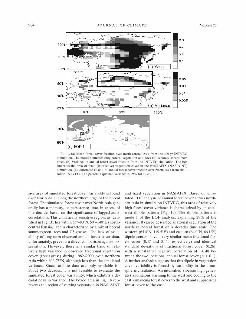
sive area of simulated forest cover variability is foundover North Asia, along the northern edge of the borealforest. The simulated forest cover over North Asia gen-erally has a memory, or persistence time, in excess ofone decade, based on the significance of lagged auto-correlations. This climatically sensitive region, as iden-tified in Fig. 1b, lies within 55°–80°N, 50°–140°E (north-central Russia), and is characterized by a mix of borealsummergreen trees and C3 grasses. The lack of avail-ability of long-term observed annual forest cover data,unfortunately, prevents a direct comparison against ob-servations. However, there is a similar band of rela-tively high variance in observed fractional vegetationcover (tree�grass) during 1982–2000 over northernAsia within 60°–75°N, although less than the simulatedvariance. Since satellite data are only available forabout two decades, it is not feasible to evaluate thesimulated forest cover variability, which exhibits a de-cadal peak in variance. The boxed area in Fig. 1b rep-resents the region of varying vegetation in NASIAINT

and fixed vegetation in NASIAFIX. Based on unro-tated EOF analysis of annual forest cover across north-ern Asia in simulation INTVEG, this area of relativelyhigh forest cover variance is characterized by an east–west dipole pattern (Fig. 1c). The dipole pattern ismode 1 of the EOF analysis, explaining 29% of thevariance. It can be described as a zonal oscillation of thenorthern boreal forest on a decadal time scale. Thewestern (65.4°N, 119.5°E) and eastern (64.0°N, 66.1°E)dipole centers have a very similar mean fractional for-est cover (0.47 and 0.45, respectively) and identicalstandard deviations of fractional forest cover (0.26),with a substantial negative correlation of �0.48 be-tween the two locations’ annual forest cover (p � 0.1).A further analysis suggests that this dipole in vegetationcover variability is forced by variability in the atmo-spheric circulation. An intensified Siberian high gener-ates anomalous warming to the west and cooling to theeast, enhancing forest cover to the west and suppressingforest cover to the east.

FIG. 1. (a) Mean forest cover fraction over north-central Asia from the 400-yr INTVEGsimulation. The model simulates only natural vegetation and does not separate shrubs fromtrees. (b) Variance in annual forest cover fraction from the INTVEG simulation. The boxindicates the area of fixed (interactive) vegetation cover in the NASIAFIX (NASIAINT)simulation. (c) Unrotated EOF-1 of annual forest cover fraction over North Asia from simu-lation INTVEG. The percent explained variance is 29% for EOF-1.

984 J O U R N A L O F C L I M A T E VOLUME 20

4. Impact of vegetation variability on oceantemperatures

Annual North Pacific SSTs from INTVEG are com-pared to observed SSTs (not shown) from both theERSST and Kaplan extended SST datasets. Despite apersistent cold bias, the model produces a reasonablemeridional gradient of annual SSTs over the North Pa-cific, including a tight gradient in the highly baroclinicKuroshio Extension region. The model and observa-tions exhibit a peak in SST variance in the KuroshioExtension and the Gulf of Alaska, although the model’svariance in the latter region is excessive due to toomuch sea ice variability there. The Pacific decadal os-cillation (PDO) pattern appears as EOF-1 in both theINTVEG simulation and observations, with oppositesigns between the west-central Pacific SSTs around40°N and SSTs along the west coast of North America.The percent explained variance of EOF-1 is 33% in theKaplan dataset and 44% in INTVEG. We concludethat FOAM-LPJ produces acceptable North PacificSST variability, as previously determined by Wu et al.(2003) and Wu and Liu (2003).

On interannual and decadal time scales, the Kuro-shio Extension exhibits the largest variability in sea sur-face and subsurface temperatures across the North Pa-

cific (Miller et al. 1998; Xie et al. 2000). It is also char-acterized by the largest heat exchanges between theocean and atmosphere across the extratropical NorthPacific (Vivier et al. 2002). The Kuroshio Extension is acritical center for the PDO (Mantua et al. 1997; Kwonand Deser 2007). We find that variability in NorthAsian forest cover can potentially impose a significantimpact on variability in the Kuroshio Extension.

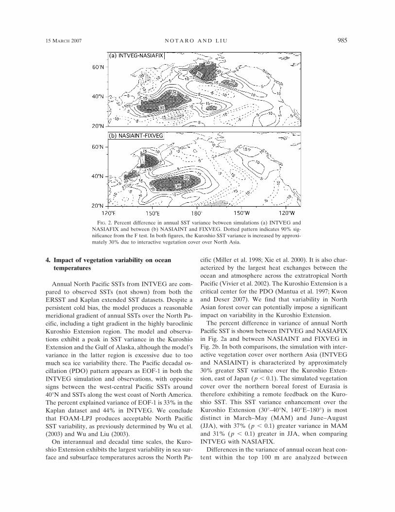
The percent difference in variance of annual NorthPacific SST is shown between INTVEG and NASIAFIXin Fig. 2a and between NASIAINT and FIXVEG inFig. 2b. In both comparisons, the simulation with inter-active vegetation cover over northern Asia (INTVEGand NASIAINT) is characterized by approximately30% greater SST variance over the Kuroshio Exten-sion, east of Japan (p � 0.1). The simulated vegetationcover over the northern boreal forest of Eurasia istherefore exhibiting a remote feedback on the Kuro-shio SST. This SST variance enhancement over theKuroshio Extension (30°–40°N, 140°E–180°) is mostdistinct in March–May (MAM) and June–August(JJA), with 37% (p � 0.1) greater variance in MAMand 31% (p � 0.1) greater in JJA, when comparingINTVEG with NASIAFIX.

Differences in the variance of annual ocean heat con-tent within the top 100 m are analyzed between

FIG. 2. Percent difference in annual SST variance between simulations (a) INTVEG andNASIAFIX and between (b) NASIAINT and FIXVEG. Dotted pattern indicates 90% sig-nificance from the F test. In both figures, the Kuroshio SST variance is increased by approxi-mately 30% due to interactive vegetation cover over North Asia.

15 MARCH 2007 N O T A R O A N D L I U 985

INTVEG and NASIAFIX. Heat content variancewithin the west-central North Pacific is enhanced by upto 35% east of Japan (p � 0.1) in INTVEG, which isattributed to remote vegetation feedbacks from north-ern Asia. The percent variance differences of the fol-lowing terms (averaged over the top 100 m) are com-puted: surface heat flux, anomalous advection, meanadvection, horizontal diffusion, and vertical diffusionand convection (Wu and Liu 2005). The enhancedocean heat content variance in INTVEG, compared toNASIAFIX, appears to be largely related to the en-hanced variance in anomalous horizontal heat advec-tion [��(�T/�y) and u�(�T/�x)] (p � 0.1). Over the Kuro-shio Extension, the variance in oceanic meridional cur-rents is enhanced in INTVEG, particularly duringMAM and JJA. In MAM, when SST variance over theKuroshio Extension is most enhanced in INTVEGcompared to NASIAFIX, there is a 22% increase invariance in anomalous meridional heat advection overthe Kuroshio Extension. These results suggest that veg-etation cover variability over northern Asia is impact-ing the atmospheric circulation pattern, thereby influ-encing meridional ocean currents and heat transportacross the North Pacific. Local surface fluxes of sen-sible and latent heat are significantly enhanced inINTVEG upstream over the Kuroshio region but notthe Kuroshio Extension, suggesting a remote contribu-tion to enhanced Kuroshio Extension SST variability.

In agreement with our findings, the dominant influenceof meridional heat advection by anomalous ocean cur-rents on SST variability in the Kuroshio Extension hasbeen noted in previous studies (Latif and Barnett 1994,1996; Seager et al. 2001; Vivier et al. 2002; Wu et al.2003; Kelly 2004; Kwon and Deser 2007), with localsurface fluxes playing less of a role (Kelly 2004).

5. Impact of vegetation variability on theatmosphere

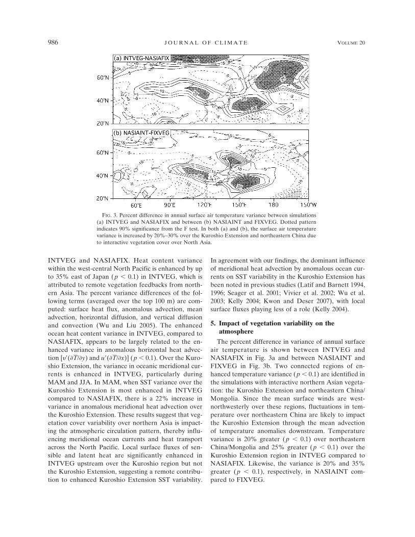
The percent difference in variance of annual surfaceair temperature is shown between INTVEG andNASIAFIX in Fig. 3a and between NASIAINT andFIXVEG in Fig. 3b. Two connected regions of en-hanced temperature variance (p � 0.1) are identified inthe simulations with interactive northern Asian vegeta-tion: the Kuroshio Extension and northeastern China/Mongolia. Since the mean surface winds are west-northwesterly over these regions, fluctuations in tem-perature over northeastern China are likely to impactthe Kuroshio Extension through the mean advectionof temperature anomalies downstream. Temperaturevariance is 20% greater (p � 0.1) over northeasternChina/Mongolia and 25% greater (p � 0.1) over theKuroshio Extension region in INTVEG compared toNASIAFIX. Likewise, the variance is 20% and 35%greater (p � 0.1), respectively, in NASIAINT com-pared to FIXVEG.

FIG. 3. Percent difference in annual surface air temperature variance between simulations(a) INTVEG and NASIAFIX and between (b) NASIAINT and FIXVEG. Dotted patternindicates 90% significance from the F test. In both (a) and (b), the surface air temperaturevariance is increased by 20%–30% over the Kuroshio Extension and northeastern China dueto interactive vegetation cover over North Asia.

986 J O U R N A L O F C L I M A T E VOLUME 20

Over the Kuroshio Extension, the variance in surfaceair temperature is 35% greater (p � 0.1) for MAM inINTVEG compared to NASIAFIX. Over northeasternChina, variance is 25% greater (p � 0.1) for Septem-ber–November (SON) in INTVEG compared toNASIAFIX. These seasonal results qualitatively agreewith the comparison of NASIAINT with FIXVEG. In-terestingly, the largest differences in temperature vari-ance between simulations are located outside the criti-cal North Asia box, suggesting substantial remote veg-etation feedbacks. Similar to studies by Bonan et al.(1995), Chase et al. (2000), Zhao et al. (2001), andLynch et al. (2003), we found that vegetation changeswithin the forest–tundra transition region over north-ern Asia can have significant widespread impacts onclimate.

6. Mechanism of remote feedback

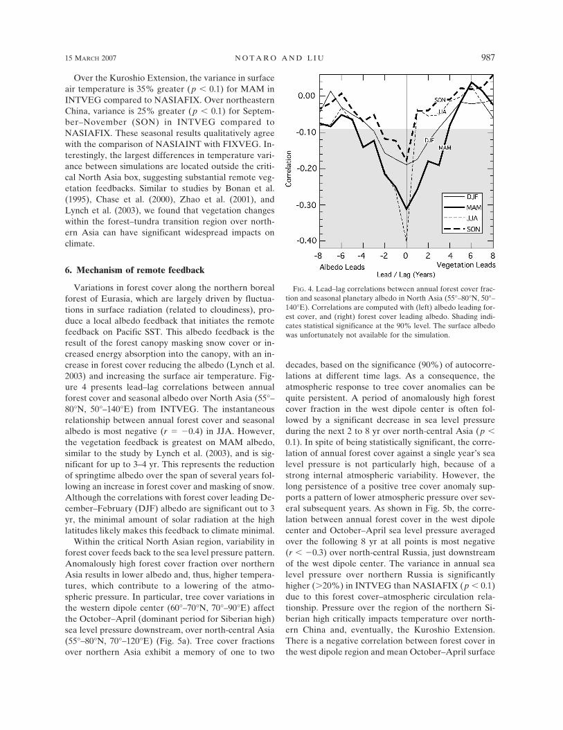
Variations in forest cover along the northern borealforest of Eurasia, which are largely driven by fluctua-tions in surface radiation (related to cloudiness), pro-duce a local albedo feedback that initiates the remotefeedback on Pacific SST. This albedo feedback is theresult of the forest canopy masking snow cover or in-creased energy absorption into the canopy, with an in-crease in forest cover reducing the albedo (Lynch et al.2003) and increasing the surface air temperature. Fig-ure 4 presents lead–lag correlations between annualforest cover and seasonal albedo over North Asia (55°–80°N, 50°–140°E) from INTVEG. The instantaneousrelationship between annual forest cover and seasonalalbedo is most negative (r � �0.4) in JJA. However,the vegetation feedback is greatest on MAM albedo,similar to the study by Lynch et al. (2003), and is sig-nificant for up to 3–4 yr. This represents the reductionof springtime albedo over the span of several years fol-lowing an increase in forest cover and masking of snow.Although the correlations with forest cover leading De-cember–February (DJF) albedo are significant out to 3yr, the minimal amount of solar radiation at the highlatitudes likely makes this feedback to climate minimal.

Within the critical North Asian region, variability inforest cover feeds back to the sea level pressure pattern.Anomalously high forest cover fraction over northernAsia results in lower albedo and, thus, higher tempera-tures, which contribute to a lowering of the atmo-spheric pressure. In particular, tree cover variations inthe western dipole center (60°–70°N, 70°–90°E) affectthe October–April (dominant period for Siberian high)sea level pressure downstream, over north-central Asia(55°–80°N, 70°–120°E) (Fig. 5a). Tree cover fractionsover northern Asia exhibit a memory of one to two

decades, based on the significance (90%) of autocorre-lations at different time lags. As a consequence, theatmospheric response to tree cover anomalies can bequite persistent. A period of anomalously high forestcover fraction in the west dipole center is often fol-lowed by a significant decrease in sea level pressureduring the next 2 to 8 yr over north-central Asia (p �0.1). In spite of being statistically significant, the corre-lation of annual forest cover against a single year’s sealevel pressure is not particularly high, because of astrong internal atmospheric variability. However, thelong persistence of a positive tree cover anomaly sup-ports a pattern of lower atmospheric pressure over sev-eral subsequent years. As shown in Fig. 5b, the corre-lation between annual forest cover in the west dipolecenter and October–April sea level pressure averagedover the following 8 yr at all points is most negative(r � �0.3) over north-central Russia, just downstreamof the west dipole center. The variance in annual sealevel pressure over northern Russia is significantlyhigher (20%) in INTVEG than NASIAFIX (p � 0.1)due to this forest cover–atmospheric circulation rela-tionship. Pressure over the region of the northern Si-berian high critically impacts temperature over north-ern China and, eventually, the Kuroshio Extension.There is a negative correlation between forest cover inthe west dipole region and mean October–April surface

FIG. 4. Lead–lag correlations between annual forest cover frac-tion and seasonal planetary albedo in North Asia (55°–80°N, 50°–140°E). Correlations are computed with (left) albedo leading for-est cover, and (right) forest cover leading albedo. Shading indi-cates statistical significance at the 90% level. The surface albedowas unfortunately not available for the simulation.

15 MARCH 2007 N O T A R O A N D L I U 987

air temperature averaged over the following 8 yr acrossa band stretching through eastern Russia, northeasternChina, Japan, and the Kuroshio Extension (Fig. 5c). Apositive forest cover anomaly over the western dipolecenter tends to lead to a weaker northern Siberian high,which limits its ability to access Arctic air masses, re-duces northerly winds and cold air advection to the eastof the high, and results in warmer conditions to thesoutheast. This establishes a link between the forestcover over northern Asia and temperatures over theKuroshio Extension.

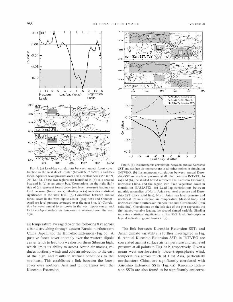
The link between Kuroshio Extension SSTs andAsian climate variability is further investigated in Fig.6. Annual Kuroshio Extension SSTs in INTVEG arecorrelated against surface air temperature and sea levelpressure at all points in Figs. 6a,b, respectively. Given amean west-northwesterly lower-tropospheric wind,temperatures across much of East Asia, particularlynortheastern China, are significantly correlated withKuroshio Extension SSTs (Fig. 6a). Kuroshio Exten-sion SSTs are also found to be significantly anticorre-

FIG. 5. (a) Lead–lag correlations between annual forest coverfraction in the west dipole center (60°–70°N, 70°–90°E) and Oc-tober–April sea level pressure over north–central Asia (55°–80°N,70°–120°E). These two regions are identified in (b) as a shadedbox and in (c) as an empty box. Correlations on the right (left)side of (a) represent forest cover (sea level pressure) leading sealevel pressure (forest cover). Shading in (a) indicates statisticalsignificance at the 90% level. (b) Correlation between annualforest cover in the west dipole center (gray box) and October–April sea level pressure averaged over the next 8 yr. (c) Correla-tion between annual forest cover in the west dipole center andOctober–April surface air temperature averaged over the next8 yr.

FIG. 6. (a) Instantaneous correlation between annual KuroshioSST and surface air temperature at all other points in simulationINTVEG. (b) Instantaneous correlation between annual Kuro-shio SST and sea level pressure at all other points in INTVEG. In(a) and (b), the shaded boxed represent the Kuroshio Extension,northeast China, and the region with fixed vegetation cover insimulation NASIAFIX. (c) Lead–lag correlations betweenmonthly anomalies of North Asian sea level pressure and Kuro-shio SST (thick solid line), North Asian sea level pressure andnortheast China’s surface air temperature (dashed line), andnortheast China’s surface air temperature and Kuroshio SST (thinsolid line). Correlations on the left side of the plot represent thefirst named variable leading the second named variable. Shadingindicates statistical significance at the 90% level. Subscripts inlegend indicate regional boxes in (a).

988 J O U R N A L O F C L I M A T E VOLUME 20

lated with sea level pressure over northern Russia (Fig.6b). The correlation pattern of Fig. 6b closely matchesthe pattern of EOF-1 for the North Asian annual sealevel pressure (41% of the variance). In particular, DJFsea level pressure over northern Russia is highly anti-correlated (r � �0.4) with the following MAM Kuro-shio Extension SST, suggesting a stronger wintertimenorthern Siberian high supporting lower springtimeKuroshio Extension SSTs. These findings reflect previ-ous studies using observational data. Panagiotopouloset al. (2005) noted that the Siberian high’s observedimpact on atmospheric circulation and temperature ex-tends over a vast area from the Arctic to the tropicalPacific, with the strength of the Siberian high negativelycorrelated with temperatures over Siberia and extend-ing southeastward to the Kuroshio Extension. Ob-served changes in sea level pressure anomalies over thenorthern Siberian high also have a strong influence onthe East Asian winter monsoon (Gong et al. 2001), witha stronger high leading to lower SSTs in the Sea ofJapan (Minobe et al. 2004).

Monthly lead–lag correlations are performed for theregions of North Asia (55°–80°N, 50°–140°E), northeastChina (38°–51°N, 105°–130°E), and the Kuroshio Ex-tension (30°–40°N, 140°E–180°) (Fig. 6c). The strongestnegative correlation between North Asia’s sea levelpressure and northeast China’s surface air temperatureis instantaneous, with a stronger northern Siberian highencouraging greater northerlies with cold advectionacross East Asia. Similarly, Gong et al. (2001) deter-mined that China’s observed wintertime temperaturesare strongly anticorrelated with sea level pressurevariations over the Eurasian high latitudes. In fact, theSiberian high accounts for 44% of the total observedwintertime temperature variance of China on average(Gong and Wang 1999). Observations reveal that, dur-ing the winter monsoon, the Siberian high producescold northerly and northwesterly winds across China,the Sea of Japan, and South China Sea (Chu et al. 2001;Gong et al. 2001).

There is a significant positive correlation betweennortheast China’s surface air temperature and Kuro-shio Extension SST, particularly with the former vari-able leading by one month. Northeast China’s air tem-peratures during DJF are particularly well correlated(r 0.4) with the following MAM Kuroshio ExtensionSSTs. Kuroshio Extension SSTs are significantly af-fected by East Asian air temperatures over the preced-ing half year, with the mean winds advecting theseanomalies over the North Pacific. Finally, North Asiansea level pressure is negatively correlated with Kuro-shio Extension SST, especially when pressure leads byone month. In summary, forest cover anomalies along

the north side of the Asian boreal forest lead to changesin albedo, which result in changes in temperature andsea level pressure. This atmospheric circulation re-sponse produces changes in air temperature over EastAsia that are later advected over the Kuroshio Exten-sion, impacting the SSTs.

The enhanced Kuroshio SST variance in INTVEGcompared to NASIAFIX results in a substantial changein variance of the large-scale atmospheric circulationover East Asia and the North Pacific (not shown). Themean annual 250-hPa winds over East Asia in INTVEGare dominated by a strong zonal jet stream across Japanwith wind speeds reaching 40 m s�1. The variance inannual wind speed peaks along the north and southsides of this jet core, particularly in the jet exit regionswhere the variance reaches 6–8 m s�1. The variance in250-hPa wind speed is enhanced by 20%–30% (p � 0.1)along the north and south sides of the upper-level jet inINTVEG compared to NASIAFIX, attributed to re-mote feedbacks from North Asian vegetation and di-rectly linked to enhanced Kuroshio SST variance. Theconsequence is greater meridional fluctuations in theposition of the East Asian upper-level jet stream, withlikely consequences on the circulation pattern acrossthe North Pacific and into North America. In an obser-vational study, Panagiotopoulos et al. (2005) likewisefound that the subtropical jet over China and the NorthPacific is stronger when the Siberian high is intense.Likewise, Lynch et al. (2003) performed an experimentin which they imposed a poleward expansion of theAsian boreal forest and found that the planetary wavepattern of the NH midlatitudes shifted poleward, illus-trating the impact of vegetation on the large-scale cir-culation pattern.

In comparing MAM 500-hPa height variance be-tween INTVEG and NASIAFIX, we determine thatthere is a 30% enhancement in height variance over theBering Sea in INTVEG, likely related to sea ice feed-backs, and a slight southward shift of the North Pacificstorm track, related to slightly lower mean tempera-tures over northern Asia and the North Pacific. There isup to a 20% reduction in MAM sea level pressure vari-ance over the Aleutian low in INTVEG.

7. Conclusions

Four simulations, using a fully coupled climate modelwith dynamic vegetation, FOAM-LPJ, are producedand analyzed to assess potential remote impacts of veg-etation variability on SST variability. The most substan-tial area of forest cover variability is simulated overNorth Asia, on the poleward side of the boreal forest,dominated by an east–west dipole pattern of forest

15 MARCH 2007 N O T A R O A N D L I U 989

cover variability. By comparing the simulationsINTVEG with NASIAFIX, and NASIAINT withFIXVEG, the impact of vegetation variability over thenorthern edge of the Asian boreal forest is isolated.Both comparisons show a robust signal of significantlyenhanced Kuroshio Extension SST variance (�30%)when annual vegetation cover is permitted to vary overnorth-central Russia. Likewise, surface air temperaturevariance is enhanced in the INTVEG and NASIAINTsimulations over the Kuroshio Extension and north-eastern China/Mongolia. A mechanism for the en-hanced variance is identified. Positive forest coveranomalies over the western dipole region of northernRussia, which tend to persist for years, reduce the al-bedo by absorbing more radiation in the canopy andmasking underlying snow cover. This lower albedo re-sults in higher surface air temperatures and, eventually,lower pressure along the northern Siberian high, whichreduces northerly winds and cold advection over north-east Asia. The mean winds then advect warm anomaliesover northeast China east-southeastward to the Kuro-shio Extension. Thus, the atmosphere serves as a bridgebetween vegetation variability over North Asia andSST variability over the North Pacific to compose aremote vegetation feedback.

While the lack of observational data of annual forestcover fraction makes it difficult to confirm these modelfindings, there are several reasons to have confidence inthe results, at least qualitatively. Both observed frac-tional vegetation cover (FVC) data and model outputshow relatively high variability in total vegetation coveron the poleward side of the Eurasian boreal forest, al-though the model’s variance appears to be too large.Using FOAM-LPJ, Notaro et al. (2005) simulated apoleward shift of the Eurasian boreal forest due to re-cent increases in atmospheric CO2, which agreed withsatellite data during the past two decades. The modelsimulates a reasonable PDO pattern, both spatially andtemporally. The simulated relationship between the Si-berian high and East Asian temperatures agrees wellwith observed studies.

Acknowledgments. The authors are grateful to Dr.Xubin Zeng for providing the satellite-based fractionalvegetation cover data. We thank Professor John Kutz-bach, Dr. Sam Levis, Mark Marohl, and two anony-mous reviewers for their helpful comments and Dr.Robert Gallimore for the use of two of his simulations.We appreciate the computer resources provided byNCAR. This work was supported by funding from theU.S. Department of Education (DOE), National Oce-anic and Atmospheric Administration (NOAA), andNational Science Foundation (NSF).

REFERENCES

Beringer, J., F. S. Chapin, C. C. Thompson, and A. D. McGuire,2005: Surface energy exchanges along a tundra-forest transi-tion and feedbacks to climate. Agric. For. Meteor., 131, 143–161.

Betts, A. K., and J. H. Ball, 1997: Albedo over the boreal forest.J. Geophys. Res., 102, 28 901–28 909.

Bonan, G. B., 2002: Ecological Climatology: Concepts and Appli-cations. Cambridge University Press, 678 pp.

——, D. Pollard, and S. L. Thompson, 1992: Effects of borealforest vegetation on global climate. Nature, 359, 716–718.

——, F. S. Chapin III, and S. L. Thompson, 1995: Boreal forestand tundra ecosystems as components of the climate system.Climatic Change, 29, 145–167.

——, S. Levis, S. Sitch, M. Vertenstein, and K. W. Oleson, 2003: Adynamic global vegetation model for use with climate mod-els: Concepts and description of simulated vegetation dynam-ics. Global Change Biol., 9, 1543–1566.

Bowers, J. D., and W. G. Bailey, 1989: Summer energy balanceregimes for alpine tundra, Plateau Mountain, Alberta,Canada. Arct. Alp. Res., 21, 135–143.

Chapin, F. S., W. Eugster, J. P. McFadden, A. H. Lynch, andD. A. Walker, 2000: Summer differences among arctic eco-systems in regional climate forcing. J. Climate, 13, 2002–2010.

Chase, T. N., R. A. Pielke, T. G. F. Kittel, R. R. Nemani, andS. W. Running, 2000: Simulated impacts of historical landcover changes on global climate in northern winter. ClimateDyn., 16, 93–105.

Chu, P. C., J. Lan, and C. Fan, 2001: Japan Sea thermohalinestructure and circulation. Part I: Climatology. J. Phys. Ocean-ogr., 31, 244–271.

Cramer, B. A., and Coauthors, 2001: Global response of terres-trial ecosystem structure and function to CO2 and climatechange: Results from six dynamic global vegetation models.Global Change Biol., 7, 357–373.

DeFries, R. S., J. R. G. Townshend, and M. C. Hansen, 1999:Continuous fields of vegetation characteristics at the globalscale at 1-km resolution. J. Geophys. Res., 104, 16 911–16 925.

——, M. C. Hansen, J. R. G. Townshend, A. C. Janetos, and T. R.Loveland, 2000: A new global 1-km dataset of percentagetree cover derived from remote sensing. Global Change Biol.,6, 247–254.

Delire, C., J. A. Foley, and S. Thompson, 2004: Long-term vari-ability in a coupled atmosphere–biosphere model. J. Climate,17, 3947–3959.

Drake, J., I. Foster, J. Michalakes, B. Toonen, and P. Worley,1995: Design and performance of a scalable parallel commu-nity climate model. Parallel Comput., 21, 1571–1591.

Gallimore, R., R. Jacob, and J. Kutzbach, 2005: Coupled atmo-sphere–ocean–vegetation simulations for modern and mid-Holocene climates: Role of extratropical vegetation coverfeedbacks. Climate Dyn., 25, 755–776.

Gong, D. Y., and S. W. Wang, 1999: Long-term variability of theSiberian High and the possible influence of global warming.Acta Geogr. Sin., 54, 125–133.

——, ——, and J.-H. Zhu, 2001: East Asian winter monsoon andArctic Oscillation. Geophys. Res. Lett., 28, 2073–2076.

Isard, S. A., and M. J. Belding, 1989: Evapotranspiration from thealpine tundra of Colorado, U.S.A. Arct. Alp. Res., 21, 71–82.

Jacob, R. L., 1997: Low frequency variability in a simulated at-

990 J O U R N A L O F C L I M A T E VOLUME 20

mosphere ocean system. Ph.D. thesis, University of Wiscon-sin—Madison, 159 pp.

Kaplan, A., M. Cane, Y. Kushnir, A. Clement, M. Blumenthal,and B. Rajagopalan, 1998: Analyses of global sea surfacetemperature 1856-1991. J. Geophys. Res., 103, 18 567–18 589.

Kelly, K. A., 2004: The relationship between oceanic heat trans-port and surface fluxes in the western North Pacific: 1970–2000. J. Climate, 17, 573–588.

Kiehl, J. T., J. J. Hack, G. B. Bonan, B. A. Boville, D. L. William-son, and P. J. Rasch, 1998: The National Center for Atmo-spheric Research Community Climate Model: CCM3. J. Cli-mate, 11, 1131–1150.

Kwon, Y.-O., and C. Deser, 2007: North Pacific decadal variabilityin the Community Climate System Model version 2. J. Cli-mate, in press.

Lafleur, P. M., and W. R. Rouse, 1995: Energy partitioning attreeline forest and tundra sites and its sensitivity to climatechange. Atmos.–Ocean, 33, 121–133.

Latif, M., and T. P. Barnett, 1994: Causes of decadal climate vari-ability over the North Pacific and North America. Science,206, 634–637.

——, and ——, 1996: Decadal climate variability over the NorthPacific and North America: Dynamics and predictability. J.Climate, 9, 2407–2423.

Liu, Z., and L. Wu, 2004: Atmospheric response to North PacificSST: The role of ocean–atmosphere coupling. J. Climate, 17,1859–1882.

——, J. Kutzbach, and L. Wu, 2000: Modeling climate shift of ElNiño in the Holocene. Geophys. Res. Lett., 27, 2265–2268.

——, B. Otto-Bliesner, J. Kutzbach, L. Li, and C. Shields, 2003:Coupled climate simulation of the evolution of global mon-soons in the Holocene. J. Climate, 16, 2472–2490.

——, M. Notaro, J. Kutzbach, and N. Liu, 2006: Assessing globalvegetation–climate feedbacks from observations. J. Climate,19, 787–814.

Lloyd, A. H., 2005: Ecological histories from Alaskan tree linesprovide insight into future change. Ecology, 86, 1687–1695.

Lundberg, A., and J. Beringer, 2005: Albedo and snowmelt ratesacross a tundra-to-forest transition. Preprints, 15th Int.Northern Research Basins Symp. and Workshop, Luleä toKvikkjokk, Sweden, Lund University, 10 pp.

Lynch, A. H., A. R. Rivers, and P. J. Bartlein, 2003: An assess-ment of the influence of land cover uncertainties on the simu-lation of global climate in the early Holocene. Climate Dyn.,21, 241–256.

Mantua, N. J., S. R. Hare, Y. Zhang, J. M. Wallace, and R. C.Francis, 1997: A Pacific interdecadal climate oscillation withimpacts on salmon production. Bull. Amer. Meteor. Soc., 78,1069–1079.

McFadden, J. P., 1998: The effects of plant growth forms on thesurface energy balance and moisture exchange of Arctic tun-dra. Ph.D. dissertation, University of California, Berkeley,123 pp. [Available from UMI Dissertation Services, 200 N.Zeeb Road, Ann Arbor, MI 48106-1346.]

McGuire, A. D., and Coauthors, 2001: Carbon balance of the ter-restrial biosphere in the twentieth century: Analyses of CO2,climate and land use effects with four process-based ecosys-tem models. Global Biogeochem. Cycles, 15, 183–206.

Miller, A. J., D. R. Cayan, and W. B. White, 1998: A westward-intensified decadal change in the North Pacific thermoclineand gyre-scale circulation. J. Climate, 11, 3112–3127.

Minobe, S., A. Sako, and M. Nakamura, 2004: Interannual tointerdecadal variability in the Japan Sea based on a new grid-

ded upper water temperature dataset. J. Phys. Oceanogr., 34,2382–2397.

Notaro, M., Z. Liu, R. Gallimore, S. J. Vavrus, J. E. Kutzbach,I. C. Prentice, and R. L. Jacob, 2005: Simulated and observedpreindustrial to modern vegetation and climate changes. J.Climate, 18, 3650–3671.

——, ——, and J. W. Williams, 2006: Observed vegetation–climate feedbacks in the United States. J. Climate, 19, 763–786.

——, S. Vavrus, and Z. Liu, 2007: Global vegetation and climatechange due to future increases in CO2 as projected by a fullycoupled model with dynamic vegetation. J. Climate, 20, 70–90.

Panagiotopoulos, F., M. Shahgedanova, A. Hannachi, and D. B.Stephenson, 2005: Observed trends and teleconnections ofthe Siberian High: A recently declining center of action. J.Climate, 18, 1411–1422.

Parker, D. E., P. D. Jones, C. K. Folland, and A. Bevan, 1994:Interdecadal changes of surface temperature since the latenineteenth century. J. Geophys. Res., 99, 14 373–14 399.

Reynolds, R. W., and T. M. Smith, 1994: Improved global sea sur-face temperature analyses. J. Climate, 7, 929–948.

Riseborough, D. W., and C. A. Burn, 1988: Influence of an or-ganic mat on the active layer. Proc. Fifth Int. Conf. on Per-mafrost, Trongheim, Norway, Tapir Publications, 633–638.

Robinson, D. A., and G. Kukla, 1985: Maximum surface albedo ofseasonally snow-covered lands in the Northern Hemisphere.J. Climate Appl. Meteor., 24, 402–411.

Rouse, W. R., D. W. Carlson, and E. J. Weick, 1992: Impacts ofsummer warming on the energy and water balance of wetlandtundra. Climatic Change, 22, 305–326.

Seager, R., Y. Kushnir, N. Naik, M. A. Cane, and J. A. Miller,2001: Wind-driven shifts in the latitude of the Kuroshio–Oyashio Extension and generation of SST anomalies on de-cadal timescales. J. Climate, 14, 4249–4265.

Shaeffer, J. D., and E. R. Reiter, 1987: Measurements of surfaceenergy budgets in the Rocky Mountains of Colorado. J. Geo-phys. Res., 92, 4145–4162.

Sitch, S., 2000: The role of vegetation dynamics in the control ofatmospheric CO2 content. Ph.D. dissertation, Lund Univer-sity, 213 pp.

——, and Coauthors, 2003: Evaluation of ecosystem dynamics,plant geography and terrestrial carbon cycling in the LPJdynamic global vegetation model. Global Change Biol., 9,161–185.

Smith, T. M., and R. W. Reynolds, 2003: Extended reconstructionof global sea surface temperatures based on COADS data(1854–1997). J. Climate, 16, 1495–1510.

——, and ——, 2004: Improved extended reconstruction of SST(1854–1997). J. Climate, 17, 2466–2477.

Snyder, P. K., C. Delire, and J. A. Foley, 2004: Evaluating theinfluence of different vegetation biomes on the global cli-mate. Climate Dyn., 23, 279–302.

Sturm, M., J. P. McFadden, G. E. Liston, F. S. Chapin III, C. H.Racine, and J. Holmgren, 2001: Snow–shrub interactions inArctic tundra: A hypothesis with climatic implications. J. Cli-mate, 14, 336–344.

Vivier, F., K. A. Kelly, and L. Thompson, 2002: Heat budget inthe Kuroshio Extension region: 1993–99. J. Phys. Oceanogr.,32, 3436–3454.

Wohlfahrt, J., S. P. Harrison, and P. Braconnot, 2004: Synergisticfeedbacks between ocean and vegetation on mid- and high-

15 MARCH 2007 N O T A R O A N D L I U 991

latitude climates during the mid-Holocene. Climate Dyn., 22,223–238.

Wu, L., and Z. Liu, 2002: Is tropical Atlantic variability driven bythe North Atlantic Oscillation? Geophys. Res. Lett., 29, 1653,doi:10.1029/2002GL014939.

——, and ——, 2003: Decadal variability in the North Pacific: Theeastern North Pacific mode. J. Climate, 16, 3111–3131.

——, and ——, 2005: North Atlantic decadal variability: Air–seacoupling, oceanic memory, and potential Northern Hemi-sphere resonance. J. Climate, 18, 331–349.

——, ——, and R. Gallimore, 2003: Pacific decadal variability:The tropical Pacific mode and North Pacific mode. J. Climate,16, 1101–1120.

Xie, S.-P., T. Kunitani, A. Kubokawa, M. Nonaka, and S. Hosoda,2000: Interdecadal thermocline variability in the North Pa-cific for 1958–97: A GCM simulation. J. Phys. Oceanogr., 30,2798–2813.

Zeng, N., and J. D. Neelin, 2000: The role of vegetation–climateinteraction and interannual variability in shaping the Africansavanna. J. Climate, 13, 2665–2670.

——, ——, K.-M. Lau, and C. J. Tucker, 1999: Enhancement ofinterdecadal climate variability in the Sahel by vegetationinteraction. Science, 286, 1537–1540.

——, K. Hales, and J. D. Neelin, 2002: Nonlinear dynamics in acoupled vegetation–atmosphere system and implications fordesert–forest gradient. J. Climate, 15, 3474–3487.

Zeng, X., R. E. Dickinson, A. Walker, M. Shaikh, R. S. DeFries,and J. Qi, 2000: Derivation and evaluation of global 1-kmfractional vegetation cover data for land modeling. J. Appl.Meteor., 39, 826–839.

Zhao, M., A. J. Pitman, and T. Chase, 2001: The impact of landcover change on the atmospheric circulation. Climate Dyn.,17, 467–477.

992 J O U R N A L O F C L I M A T E VOLUME 20