B O N N E V I L L E P O W E R A D M I N I S T R A T I O N

BP-14 Final Rate Proposal

Power Risk and Market Price Study

BP-14-FS-BPA-04

July 2013

BP-14-FS-BPA-04

Page i

TABLE OF CONTENTS

Page

COMMONLY USED ACRONYMS AND SHORT FORMS ..................................................... vii

1. INTRODUCTION ...............................................................................................................1

1.1 Purpose of the Power Risk and Market Price Study ................................................1 1.1.1 BPA’s Treasury Payment Probability Standard ...........................................2 1.1.2 How Risk and Market Price Results Are Used ............................................4

1.2 Overview of Risk Assessment and Mitigation.........................................................6 1.2.1 Risk Mitigation Objectives ..........................................................................6

1.2.2 Quantitative and Qualitative Risk Assessment and Mitigation ...................7

1.2.2.1 Overview of Quantitative Risk Assessment ..................................8

1.2.2.2 Overview of Quantitative Risk Mitigation ....................................8

1.2.2.3 Overview of Qualitative Risk Assessment and Mitigation ...........9

2. QUANTITATIVE RISK ASSESSMENT .........................................................................11 2.1 Introduction ............................................................................................................11

2.2 Study Models .........................................................................................................11 2.2.1 @RISK Computer Software ......................................................................12

2.2.2 R Statistical Software .................................................................................12 2.2.3 AURORAxmp............................................................................................13

2.2.3.1 Operating Risk Models................................................................13

2.2.3.2 Revenue Simulation Model (RevSim) ........................................14

2.2.4 Non-Operating Risk Model........................................................................15 2.2.4.1 NORM Methodology ..................................................................16 2.2.4.2 Data Gathering and Development of Probability

Distributions ................................................................................16 2.3 AURORAxmp Model Inputs .................................................................................17

2.3.1 Natural Gas Prices Used in AURORAxmp ...............................................17 2.3.1.1 Methodology for Deriving AURORAxmp Zone Natural

Gas Prices....................................................................................17 2.3.1.2 Recent Natural Gas Market Fundamentals..................................19 2.3.1.3 Henry Hub Forecast ....................................................................21 2.3.1.4 The Basis Differential Forecast ...................................................26 2.3.1.5 Natural Gas Price Risk ................................................................27

2.3.2 Load Forecasts Used in AURORAxmp .....................................................28

2.3.2.1 Load Forecast ..............................................................................29

2.3.2.2 Load Risk Model .........................................................................29 2.3.2.3 Yearly Load Model .....................................................................29 2.3.2.4 Monthly Load Risk......................................................................30

2.3.3 Hourly Load Risk .......................................................................................31 2.3.4 Hydroelectric Generation ...........................................................................31

2.3.4.1 PNW Hydro Generation Risk ......................................................31 2.3.4.2 British Columbia (BC) Hydro Generation Risk ..........................32

BP-14-FS-BPA-04

Page ii

2.3.4.3 California Hydro Generation Risk ..............................................33 2.3.4.4 Hydro Shaping.............................................................................33

2.3.5 Hourly Shape of Wind Generation ............................................................34 2.3.5.1 PNW Hourly Wind Generation Risk ...........................................35

2.3.6 Thermal Plant Generation ..........................................................................35 2.3.6.1 Columbia Generating Station Generation Risk ...........................36

2.3.7 Generation Additions Due to WECC-Wide Renewable Portfolio

Standards (RPS) .........................................................................................36 2.3.8 Transmission Capacity Availability ...........................................................37

2.3.8.1 PNW Hourly Intertie Availability Risk .......................................37 2.4 Market Price Forecasts Produced By AURORAxmp ............................................38 2.5 Inputs to RevSim....................................................................................................38

2.5.1 Deterministic Data .....................................................................................39 2.5.1.1 Loads and Resources ...................................................................39 2.5.1.2 Miscellaneous Revenues .............................................................39

2.5.1.3 Composite, Load Shaping, and Demand Revenue ......................39 2.5.2 Risk Data ....................................................................................................40

2.5.2.1 Federal Hydro Generation Risk...................................................40 2.5.2.2 BPA Load Risk............................................................................42 2.5.2.3 CGS Generation Risk ..................................................................43

2.5.2.4 PS Wind Generation Risk ...........................................................43 2.5.2.5 PS Transmission and Ancillary Services Expense Risk..............45

2.5.2.6 Electricity Price Risk (Market Price and Critical Water

AURORAxmp Runs) ..................................................................46

2.6 RevSim Model Outputs..........................................................................................47 2.6.1 4(h)(10)(C) Credits ....................................................................................47

2.6.2 System Augmentation Costs ......................................................................48 2.6.3 Surplus Energy Sales/Revenues and Balancing Power

Purchases/Expenses ...................................................................................50

2.6.4 Net Revenue ...............................................................................................52 2.7 Inputs to NORM ....................................................................................................53

2.7.1 CGS Operations and Maintenance (O&M)................................................53 2.7.2 Corps of Engineers and Bureau of Reclamation O&M .............................54

2.7.3 Conservation Expense ................................................................................55 2.7.4 Spokane Settlement ....................................................................................56 2.7.5 Power Services Transmission Acquisition and Ancillary Services ...........56 2.7.6 Power Services Internal Operations Expenses ...........................................57

2.7.7 Fish & Wildlife Expenses ..........................................................................58 2.7.7.1 BPA Direct Program Costs for Fish and Wildlife

Expenses .....................................................................................58

2.7.7.2 U.S. Fish and Wildlife (USF&W) Service Lower Snake

River Hatcheries Expenses .........................................................59 2.7.7.3 Bureau of Reclamation Leavenworth Complex O&M

Expenses .....................................................................................59

BP-14-FS-BPA-04

Page iii

2.7.7.4 Corps of Engineers Fish Passage Facilities Expenses .................59 2.7.8 Court-Ordered Spill Risk ...........................................................................60 2.7.9 Interest Expense Risk .................................................................................61 2.7.10 CGS Refueling Outage Risk ......................................................................62

2.7.11 Revenue from Sales of Variable Energy Resource Balancing

Services (VERBS) .....................................................................................63 2.7.12 Operating Reserve Revenue Risk ..............................................................64 2.7.13 The Accrual-to-Cash (ATC) Adjustment...................................................66

2.8 NORM Results .......................................................................................................67

3. QUANTITATIVE RISK MITIGATION ...........................................................................69 3.1 Introduction ............................................................................................................69

3.2 Risk Mitigation Tools ............................................................................................70 3.2.1 Liquidity .....................................................................................................70

3.2.1.1 PS Reserves .................................................................................70 3.2.1.2 The Treasury Facility ..................................................................71

3.2.1.3 Within-Year Liquidity Need .......................................................71 3.2.1.4 Liquidity Reserves Level ............................................................72

3.2.1.5 Liquidity Borrowing Level..........................................................72 3.2.1.6 Net Reserves ................................................................................72

3.2.2 Planned Net Revenues for Risk .................................................................73

3.2.3 The Cost Recovery Adjustment Clause (CRAC).......................................73 3.2.3.1 Description of the CRAC ............................................................74

3.2.3.2 Administrator’s Discretion to Reduce the CRAC .......................75

3.2.4 The NFB Adjustment .................................................................................75

3.2.5 Dividend Distribution Clause (DDC) ........................................................76 3.3 Overview of the ToolKit ........................................................................................76

3.4 ToolKit Inputs and Assumptions ...........................................................................77 3.4.1 RevSim Results ..........................................................................................77 3.4.2 Non-Operating Risk Model........................................................................78

3.4.3 Treatment of Treasury Deferrals ................................................................78 3.4.4 Starting PS Reserves ..................................................................................78 3.4.5 Starting ANR .............................................................................................78 3.4.6 PS Liquidity Reserves Level ......................................................................79

3.4.7 Treasury Facility ........................................................................................79 3.4.8 Interest Rate Earned on Reserves ..............................................................79 3.4.9 Interest Credit Assumed in Net Revenue ...................................................79

3.4.10 The Cash Timing Adjustment ....................................................................80 3.4.11 Cash Lag for PNRR ...................................................................................80

3.5 Quantitative Risk Mitigation Results .....................................................................81 3.5.1 TPP .............................................................................................................81

3.5.2 Ending PS Reserves ...................................................................................81 3.5.3 CRAC and DDC ........................................................................................82

BP-14-FS-BPA-04

Page iv

4. QUALITATIVE RISK ASSESSMENT AND MITIGATION .........................................83 4.1 Introduction ............................................................................................................83 4.2 FCRPS Biological Opinion Risks ..........................................................................83

4.2.1 The NFB Adjustment .................................................................................85

4.2.2 The Emergency NFB Surcharge ................................................................85 4.2.3 Multiple NFB Trigger Events ....................................................................86

4.3 Risks Associated with Tier 2 Rate Design .............................................................87 4.3.1 Introduction ................................................................................................87 4.3.2 Identification and Analysis of Risks ..........................................................87

4.3.2.1 Risk: The Contracted-for Power Is Not Delivered to BPA ........88 4.3.2.2 Risk: A Tier 2 Customer’s Load is Lower than the

Amount Forecast .........................................................................88

4.3.2.3 Risk: A Tier 2 Customer’s Load is Higher than the

Amount Forecast .........................................................................89 4.3.2.4 Risk: A Customer Does Not Pay for its Service at the

Tier 2 Rate...................................................................................90 4.3.2.5 Risk: A Customer’s Above-RHWM Load is Lower than

its Take-or-Pay VR1-2014 Rate Amounts ..................................90 4.4 Risks Associated with Resource Support Services Rate Design ...........................91

4.4.1 Introduction ................................................................................................91

4.4.2 Identification and Analysis of Risks ..........................................................91 4.5 Qualitative Risk Assessment Results .....................................................................92

4.5.1 Biological Opinion Risks ...........................................................................92 4.5.2 Risks Associated with Tier 2 Rate Design .................................................92

4.5.3 Risks Associated with Resource Support Services Rate Design ...............93

TABLES AND FIGURES .............................................................................................................95

TABLES

Table 1: Cash Prices at Henry Hub and Basis Differentials (nominal $/MMBtu) ...............97 Table 2: Natural Gas Price Risk Model Percentiles (Nominal Henry Hub) ........................97 Table 3: Average Market Price from the Market Price Run for FY14/FY15 ......................98

Table 4: Average Market Price from AURORAxmp Critical Water Run for

FY14/FY15 ............................................................................................................98 Table 5: RevSim Net Revenue Statistics (With PNRR of $0 million) ................................99

Table 6: Risk Modeling Accrual To Cash Adjustments (in $Millions) .............................100 Table 7: CRAC Annual Thresholds and Caps ...................................................................101 Table 8: DDC Thresholds and Caps...................................................................................101 Table 9: ToolKit Summary Statistics .................................................................................102

BP-14-FS-BPA-04

Page v

FIGURES

Figure 1: Risk Assessment Information Flow .....................................................................103 Figure 2: AURORAxmp Zonal Topology ...........................................................................104 Figure 3: Basis Locations ....................................................................................................105

Figure 4: January 2012 through June 2013 Henry Hub Gas prices .....................................106 Figure 5: Winter 2011-12 statistics .....................................................................................106 Figure 6: Natural Gas Storage trend, ca. April 2012 ...........................................................107 Figure 7: Natural Gas Storage trend, June 14, 2013 ............................................................107 Figure 8: Rig Counts and Production ..................................................................................108

Figure 9: Historical Coal Prices ..........................................................................................108 Figure 10: Sumas Imports .....................................................................................................109

This page intentionally left blank.

BP-14-FS-BPA-04

Page vii

COMMONLY USED ACRONYMS AND SHORT FORMS

AAC Anticipated Accumulation of Cash

AGC Automatic Generation Control

ALF Agency Load Forecast (computer model)

aMW average megawatt(s)

AMNR Accumulated Modified Net Revenues

ANR Accumulated Net Revenues

ASC Average System Cost

BiOp Biological Opinion

BPA Bonneville Power Administration

Btu British thermal unit

CDD cooling degree day(s)

CDQ Contract Demand Quantity

CGS Columbia Generating Station

CHWM Contract High Water Mark

COE, Corps, or USACE U.S. Army Corps of Engineers

Commission Federal Energy Regulatory Commission

Corps, COE, or USACE U.S. Army Corps of Engineers

COSA Cost of Service Analysis

COU consumer-owned utility

Council or NPCC Northwest Power and Conservation Council

CP Coincidental Peak

CRAC Cost Recovery Adjustment Clause

CSP Customer System Peak

CT combustion turbine

CY calendar year (January through December)

DDC Dividend Distribution Clause

dec decrease, decrement, or decremental

DERBS Dispatchable Energy Resource Balancing Service

DFS Diurnal Flattening Service

DOE Department of Energy

DSI direct-service industrial customer or direct-service industry

DSO Dispatcher Standing Order

EIA Energy Information Administration

EIS Environmental Impact Statement

EN Energy Northwest, Inc.

EPP Environmentally Preferred Power

ESA Endangered Species Act

e-Tag electronic interchange transaction information

FBS Federal base system

FCRPS Federal Columbia River Power System

FCRTS Federal Columbia River Transmission System

BP-14-FS-BPA-04

Page viii

FELCC firm energy load carrying capability

FHFO Funds Held for Others

FORS Forced Outage Reserve Service

FPS Firm Power Products and Services (rate)

FY fiscal year (October through September)

GARD Generation and Reserves Dispatch (computer model)

GEP Green Energy Premium

GRSPs General Rate Schedule Provisions

GTA General Transfer Agreement

GWh gigawatthour

HDD heating degree day(s)

HLH Heavy Load Hour(s)

HOSS Hourly Operating and Scheduling Simulator (computer model)

HYDSIM Hydrosystem Simulator (computer model)

ICE Intercontinental Exchange

inc increase, increment, or incremental

IOU investor-owned utility

IP Industrial Firm Power (rate)

IPR Integrated Program Review

IRD Irrigation Rate Discount

IRM Irrigation Rate Mitigation

IRMP Irrigation Rate Mitigation Product

JOE Joint Operating Entity

kW kilowatt (1000 watts)

kWh kilowatthour

LDD Low Density Discount

LLH Light Load Hour(s)

LRA Load Reduction Agreement

Maf million acre-feet

Mid-C Mid-Columbia

MMBtu million British thermal units

MNR Modified Net Revenues

MRNR Minimum Required Net Revenue

MW megawatt (1 million watts)

MWh megawatthour

NCP Non-Coincidental Peak

NEPA National Environmental Policy Act

NERC North American Electric Reliability Corporation

NFB National Marine Fisheries Service (NMFS) Federal Columbia

River Power System (FCRPS) Biological Opinion (BiOp)

NLSL New Large Single Load

NMFS National Marine Fisheries Service

BP-14-FS-BPA-04

Page ix

NOAA Fisheries National Oceanographic and Atmospheric Administration

Fisheries

NORM Non-Operating Risk Model (computer model)

Northwest Power Act Pacific Northwest Electric Power Planning and Conservation

Act

NPCC or Council Pacific Northwest Electric Power and Conservation Planning

Council

NPV net present value

NR New Resource Firm Power (rate)

NT Network Transmission

NTSA Non-Treaty Storage Agreement

NUG non-utility generation

NWPP Northwest Power Pool

OATT Open Access Transmission Tariff

O&M operation and maintenance

OATI Open Access Technology International, Inc.

OMB Office of Management and Budget

OY operating year (August through July)

PF Priority Firm Power (rate)

PFp Priority Firm Public (rate)

PFx Priority Firm Exchange (rate)

PNCA Pacific Northwest Coordination Agreement

PNRR Planned Net Revenues for Risk

PNW Pacific Northwest

POD Point of Delivery

POI Point of Integration or Point of Interconnection

POM Point of Metering

POR Point of Receipt

Project Act Bonneville Project Act

PRS Power Rates Study

PS BPA Power Services

PSW Pacific Southwest

PTP Point to Point Transmission (rate)

PUD public or people’s utility district

RAM Rate Analysis Model (computer model)

RAS Remedial Action Scheme

RD Regional Dialogue

REC Renewable Energy Certificate

Reclamation or USBR U.S. Bureau of Reclamation

REP Residential Exchange Program

RevSim Revenue Simulation Model (component of RiskMod)

RFA Revenue Forecast Application (database)

RHWM Rate Period High Water Mark

BP-14-FS-BPA-04

Page x

RiskMod Risk Analysis Model (computer model)

RiskSim Risk Simulation Model (component of RiskMod)

ROD Record of Decision

RPSA Residential Purchase and Sale Agreement

RR Resource Replacement (rate)

RRS Resource Remarketing Service

RSS Resource Support Services

RT1SC RHWM Tier 1 System Capability

RTO Regional Transmission Operator

SCADA Supervisory Control and Data Acquisition

SCS Secondary Crediting Service

Slice Slice of the System (product)

T1SFCO Tier 1 System Firm Critical Output

TCMS Transmission Curtailment Management Service

TOCA Tier 1 Cost Allocator

TPP Treasury Payment Probability

TRAM Transmission Risk Analysis Model

Transmission System Act Federal Columbia River Transmission System Act

TRL Total Retail Load

TRM Tiered Rate Methodology

TS BPA Transmission Services

TSS Transmission Scheduling Service

UAI Unauthorized Increase

ULS Unanticipated Load Service

USACE, Corps, or COE U.S. Army Corps of Engineers

USBR or Reclamation U.S. Bureau of Reclamation

USFWS U.S. Fish and Wildlife Service

VERBS Variable Energy Resources Balancing Service (rate)

VOR Value of Reserves

VR1-2014 First Vintage rate of the BP-14 rate period

WECC Western Electricity Coordinating Council (formerly WSCC)

WIT Wind Integration Team

WSPP Western Systems Power Pool

BP-14-FS-BPA-04

Page 1

1. INTRODUCTION 1

The Bonneville Power Administration’s (BPA) business environment is replete with uncertainty 2

that a rigorous ratesetting process must consider. The objective of the risk study is to identify, 3

model, and analyze the impacts that key risks and risk mitigation tools have on Power Services’ 4

(PS) net revenue (total revenue less total expenses) and cash flow. The risk study is meant to 5

ensure that power rates are set high enough that the probability that BPA can meet its cash 6

obligations is at least as high as required by BPA’s Treasury Payment Probability (TPP) 7

standard. This evaluation is carried out in two distinct steps: a risk assessment step, in which the 8

distributions, or profiles, of operating and non-operating risks are defined, and a risk mitigation 9

step, in which risk mitigation tools are assessed with respect to their ability to recover power 10

costs given these uncertainties. The risk assessment estimates both the central tendency of risks 11

and the potential variability of those risks. Both of these elements are used in the ratemaking 12

process. 13

14

In this study the words “risk” and “uncertainty” are used in similar ways. Generally, each can 15

have both up-side and down-side possibilities, that is, both beneficial and harmful impacts on 16

BPA objectives. The BPA objectives that may be affected by the risks considered in this study 17

are generally BPA’s financial objectives. 18

19

1.1 Purpose of the Power Risk and Market Price Study 20

The Power Risk and Market Price Study (Study) characterizes the market price and PS net 21

revenue distributions and demonstrates that the rates and risk mitigation tools together meet 22

BPA’s standard for financial risk tolerance, the TPP standard. This Study presents the natural 23

gas price forecast, the electricity market price forecast, the quantitative and qualitative analysis 24

BP-14-FS-BPA-04

Page 2

of risks to PS net revenue, and tools for mitigating those risks. It also establishes the adequacy 1

of those tools for meeting BPA’s TPP standard. 2

3

1.1.1 BPA’s Treasury Payment Probability Standard 4

In the WP-93 rate proceeding, BPA adopted and implemented its 10-Year Financial Plan, which 5

included a policy requiring that BPA set rates to achieve a high probability of meeting its 6

payment obligations to the U.S. Treasury (Treasury). 1993 Final Rate Proposal Administrator’s 7

Record of Decision (ROD), WP-93-A-02, at 72. The specific standard set in the 10-Year 8

Financial Plan was a 95 percent probability of making both of the annual Treasury payments in 9

the two-year rate period on time and in full. This TPP standard was established as a rate period 10

standard; that is, it focuses upon the probability that BPA can successfully make all of its 11

payments to Treasury over the entire rate period, not the probability for a single year. The 12

10-Year Financial Plan was updated July 31, 2008, and remains in effect. See 13

http://www.bpa.gov/Finance/FinancialInformation/FinancialPlan/Pages/default.aspx. 14

15

The Pacific Northwest Electric Power Planning and Conservation Act (Northwest Power Act) 16

states that BPA’s payments to Treasury are the lowest priority for revenue application, meaning 17

that payments to Treasury are the first to be missed if financial reserves are insufficient to pay all 18

bills on time. 16 U.S.C. § 839e (a)(2)(A). Therefore, TPP is a prospective measure of BPA’s 19

overall ability to meet its financial obligations. 20

21

The following items (explained in more detail in section 3 of this Study) are included in the 22

calculation of TPP: 23

(1) Starting PS Reserves (Starting Financial Reserves Available for Risk Attributed to 24

PS). Financial reserves comprise cash and investment instruments held in the 25

BP-14-FS-BPA-04

Page 3

Bonneville Fund and the deferred borrowing balance. Financial reserves 1

available for risk do not include funds held for others. For example, amounts in 2

the Bonneville Fund that were collected from customers after BPA stopped 3

making payments for Residential Exchange benefits in FY 2007 that will be 4

distributed eventually are excluded. Deferred borrowing amounts exist when 5

planned borrowing has not yet been completed. When the borrowing is 6

completed, cash in the Bonneville Fund is increased and the deferred borrowing 7

balance is reduced by the same amount, leaving financial reserves unchanged. 8

(2) Planned Net Revenues for Risk. PNRR is the final component of the revenue 9

requirement that may be added to annual expenses. PNRR is needed only when 10

the risk mitigation provided by starting financial reserves and other risk 11

mitigation tools is not sufficient to meet the TPP standard. 12

(3) BPA’s Treasury Facility. The Treasury Facility is an arrangement that BPA has 13

with the U.S. Treasury, allowing BPA to borrow up to $750 million on a short-14

term basis. The full $750 million in the Treasury Facility is considered to be 15

available for the liquidity needs associated with PS. The Treasury Facility 16

functions similar to additional financial reserves. 17

(4) Within-year Liquidity Need. The within-year liquidity need is an amount of cash 18

or short-term borrowing capability that must be set aside for meeting within-year 19

liquidity needs (or risks). The $300 million amount assumed for setting the 20

BP-12 rates has been increased to $320 million for the BP-14 Final Proposal to 21

provide assurance that BPA will have sufficient liquidity to meet up to 22

$20 million of possible outstanding margin calls required by BPA’s trading of 23

financial instruments. 24

25

BP-14-FS-BPA-04

Page 4

(5) Liquidity Reserves Level. The liquidity reserves level is the amount of PS 1

Reserves that is allocated for meeting the within-year liquidity need. For this 2

Study, the liquidity reserves level is $0. 3

(6) Liquidity Borrowing Level. The liquidity borrowing level is the amount of the 4

Treasury Facility set aside to meet the within-year liquidity need. For this Study, 5

the liquidity borrowing level is $320 million. This leaves $430 million of the 6

Treasury Facility available for year-to-year liquidity needs (i.e., TPP needs). 7

(7) Cost Recovery Adjustment Clause. The CRAC is an upward adjustment to the 8

applicable power and transmission rates. The adjustment is applied to rates 9

charged for service beginning in October following a fiscal year in which PS 10

Accumulated Net Revenue (ANR) falls below the CRAC threshold. The 11

threshold is set at the ANR equivalent of $0 in financial reserves available for risk 12

attributed to PS. See Power Rate Schedules and General Rate Schedule 13

Provisions (GRSPs), BP-14-A-03-AP01, GRSP II.C. 14

(8) Dividend Distribution Clause. The DDC is a downward adjustment to the 15

applicable power and transmission rates. The adjustment is applied to rates 16

charged for service beginning in October following a fiscal year in which ANR is 17

above the DDC threshold. The threshold is set at the ANR equivalent of 18

$750 million in financial reserves available for risk attributed to PS. See 19

GRSP II.E. 20

21

1.1.2 How Risk and Market Price Results Are Used 22

The main result from the risk assessment and mitigation process is the TPP calculation. If this 23

number is 95 percent or higher, then the rates and risk mitigation tools meet BPA’s TPP 24

standard. The results also include the thresholds and caps for the CRAC and the DDC. These 25

BP-14-FS-BPA-04

Page 5

values are incorporated in the General Rate Schedule Provisions and will be applied in later 1

calculations outside the ratesetting process for determining whether a CRAC or DDC will be 2

applied to certain power and transmission rates for FY 2014 or FY 2015. 3

4

Forecasts of electricity market prices are used in the Power Rates Study, BP-14-FS-BPA-01, for: 5

(a) Prices for surplus sales and balancing purchases 6

(b) Prices for augmentation purchases 7

(c) Load Shaping rates 8

(d) Load Shaping True-up rate 9

(e) Resource Shaping rates 10

(f) Resource Support Services (RSS) rates 11

(g) Shaping the Demand rates used for the Priority Firm Power (PF), Industrial Firm 12

Power (IP), and New Resources (NR) rate schedules 13

(h) PF Tier 2 Balancing Credit 14

(i) PF Unused Rate Period High Water Mark (RHWM) Credit 15

(j) Scaling PF Tier 1 Equivalent rates 16

(k) Scaling PF Melded rates 17

(l) Balancing Augmentation Credit 18

(m) Scaling IP energy rates 19

(n) Scaling NR energy rates 20

(o) Energy Shaping Service of the New Large Single Load (NLSL) True-Up rate 21

22

The electricity market price forecast also is used in the Generation Inputs Study, BP-14-23

FS-BPA-05, to value the energy in synchronous condensing, generation dropping, and station 24

BP-14-FS-BPA-04

Page 6

service; in section 2 of this Study for the risk assessment; and for setting the Average System 1

Costs (ASCs) (which occur in separate ASC processes) that are used in ratesetting. 2

3

1.2 Overview of Risk Assessment and Mitigation 4

The risk study uses a set of models, shown in Figure 1. These models are further described 5

throughout the course of the Study. 6

7

1.2.1 Risk Mitigation Objectives 8

The following policy objectives guide the development of the risk mitigation package: 9

(a) Create a rate design and risk mitigation package that meets BPA financial 10

standards, particularly achieving a 95 percent two-year Treasury Payment 11

Probability. 12

(b) Produce the lowest possible rates, consistent with sound business principles and 13

statutory obligations, including BPA’s long-term responsibility to invest in and 14

maintain the aging infrastructure of the Federal Columbia River Power System 15

(FCRPS). 16

(c) Set lower, but adjustable, effective rates rather than higher, more stable rates. 17

(d) Include in the risk mitigation package only those elements that can be relied upon. 18

(e) Do not let financial reserve levels build up to unnecessarily high levels. 19

(f) Allocate costs and risks of products to the rates for those products to the fullest 20

extent possible; in particular, prevent any risks arising from Tier 2 service from 21

imposing costs on Tier 1 or requiring stronger Tier 1 risk mitigation. 22

(g) Rely prudently on liquidity tools, and create means to replenish them when they 23

are used in order to maintain long-term availability. 24

25

BP-14-FS-BPA-04

Page 7

It is important to understand that these objectives are not completely independent and may 1

sometimes conflict with each other. Thus, BPA must create a balance among these objectives 2

when developing its overall risk mitigation strategy. 3

4

1.2.2 Quantitative and Qualitative Risk Assessment and Mitigation 5

This Study distinguishes between quantitative and qualitative perspectives of risk. The 6

quantitative risk assessment is a set of quantitative risk simulations that are modeled using a 7

Monte Carlo approach, a statistical technique in which deterministic analysis is performed on a 8

distribution of inputs, resulting in a distribution of outputs suitable for analysis. The output from 9

the quantitative risk assessment is a set of 3,200 possible financial results (net revenues) for each 10

of the two years in the rate period (fiscal years (FY) 2014–2015) and for the year preceding the 11

rate period (FY 2013). The models used in the quantitative risk assessment are described in 12

section 2 of this Study. 13

14

The 3,200 games from the quantitative risk assessment are used in the quantitative risk 15

mitigation step to determine if BPA’s financial risk standard, the 95 percent TPP standard, has 16

been met. The model used for the quantitative risk mitigation step is described in section 3 of 17

this Study. 18

19

BPA faces some risks that are incorporated into the risk assessment and mitigation in qualitative 20

rather than quantitative ways. For the most part, the qualitative risk assessment comprises 21

logical assessments of possible events that could have significant financial consequences for 22

BPA. The qualitative risk mitigation describes measures BPA has put in place, or responses 23

BPA would make, to these events, and then presents logical analyses of whether any significant 24

BP-14-FS-BPA-04

Page 8

residual financial risk remains for BPA after taking into account the existing or newly adopted 1

mitigation measures. The qualitative risk assessment is described in section 4 of this Study. 2

3

All of these analyses work together so that BPA develops rates that recover all of its costs and 4

provide a high probability of making its Treasury payments on time and in full during the rate 5

period. 6

7

1.2.2.1 Overview of Quantitative Risk Assessment 8

The quantitative risk assessment is performed using models that quantify uncertainty. There is 9

uncertainty in market prices, reflecting the uncertainty inherent in the fundamental drivers; e.g., 10

the natural gas price. There is uncertainty in the amount of surplus power that BPA will have 11

available for secondary sales. There is uncertainty in the costs faced by BPA beyond expenses 12

related to operation of the system; e.g., fish and wildlife-related expenses. These uncertainties 13

affect the PS net revenue. 14

15

Projections of market prices for electricity are used for many aspects of setting power rates, 16

including the quantitative analysis of risk, presented in section 2 of the Study. This Study 17

explains the data used for constructing the probabilistic market price forecast and how those data 18

are used in generating the PS net revenue forecast. 19

20

1.2.2.2 Overview of Quantitative Risk Mitigation 21

BPA’s primary tool for managing the financial risks it faces is financial reserves. Since the 22

WP-02 rate proceeding, BPA has included in its rate proposals cost recovery adjustment clauses 23

that can adjust power rates between rate proceedings. These clauses add additional risk 24

mitigation to that provided by financial reserves. In this rate proceeding, the CRAC, DDC, and 25

BP-14-FS-BPA-04

Page 9

National Marine Fisheries Service, Federal Columbia River Power System, Biological Opinion 1

(NFB) Mechanisms will apply to certain Transmission rates for Ancillary and Control Area 2

Services. When financial reserves available for risk plus the additional revenue earned through 3

the CRAC do not provide sufficient risk mitigation to meet the 95 percent TPP standard, PNRR 4

is added to the revenue requirement. This increases power rates, which generate additional 5

reserves. This Study documents the risk mitigation package included in the BP-14 power rates. 6

See section 1.2.1 for a discussion of the main policy objectives considered when developing this 7

risk mitigation package. 8

9

1.2.2.3 Overview of Qualitative Risk Assessment and Mitigation 10

Financial uncertainty that is not quantitatively modeled, and any mitigation measures for these 11

risks, are described in section 4 of this Study. There are three primary categories of qualitative 12

risks in this Study: risks associated with FCRPS Biological Opinions; risks associated with 13

Tier 2 rate design; and risks associated with Resource Support Services. Biological Opinion 14

risks are mitigated through the NFB Mechanisms described in this Study and GRSP II.N. 15

16

17

18

19

20

21

22

23

24

25

This page intentionally left blank.

BP-14-FS-BPA-04

Page 11

2. QUANTITATIVE RISK ASSESSMENT 1

2.1 Introduction 2

This section describes the uncertainties pertaining to Power Services, and hence BPA’s financial 3

risk in the context of setting power rates. Section 3 describes how BPA determines whether its 4

risk mitigation measures are sufficient to meet the TPP standard given the risks detailed in this 5

section. 6

7

Variability in PS net revenue, a product of uncertainty in both power generation and market 8

prices, is substantial. BPA also considers uncertainty in (1) customer load; (2) Columbia 9

Generating Station (CGS) output; (3) wind generation; (4) system augmentation costs; (5) PS 10

transmission and ancillary services expenses; and (6) 4(h)(10)(C) credits. The effects of these 11

risk factors on PS net revenue are quantified in this Study. 12

13

PS also faces risks not directly related to the operation of the power system. These non-14

operating risks are modeled in the Non-Operating Risk Model (NORM). These risks include the 15

potential for CGS, Corps of Engineers (USACE), and U.S. Bureau of Reclamation (USBR) 16

operations and maintenance (O&M) spending to differ from their forecasts. NORM also 17

accounts for variability in interest rate expense. NORM models variability in net revenues, 18

including uncertainty due to possible court orders related to the 2008 FCRPS BiOp and 19

uncertainty in the length of the CGS refueling outages in FY 2013 and FY 2015. 20

21

2.2 Study Models 22

BPA traditionally models risks using Monte Carlo simulation. Accordingly, AURORAxmp, 23

NORM, and ToolKit each run 3,200 iterations, or games. AURORAxmp estimates electricity 24

prices, which serve as inputs to numerous other studies, including this Study. RevSim (see 25

BP-14-FS-BPA-04

Page 12

section 2.2.3.2) combines Federal system generation with prices from AURORAxmp, as well as 1

4(h)(10)(c) credits and other revenues and expenses, to produce 3,200 values for net revenue. 2

The output of this process is combined with the distribution of output from NORM and provided 3

to ToolKit, which calculates TPP. If TPP is below the 95 percent standard required by BPA’s 4

10-Year Financial Plan, then one of several risk mitigation tools may be adjusted until the 5

standard is met. These options include (1) raising the CRAC threshold, which makes it more 6

likely that the CRAC will trigger; (2) increasing the cap on the annual revenue the CRAC can 7

collect; and/or (3) adding PNRR to the revenue requirement. 8

9

2.2.1 @RISK Computer Software 10

NORM is maintained in Microsoft Excel with the add-in risk simulation computer package 11

@RISK, a product of Palisade Corporation, Ithaca, NY. @RISK allows analysts to develop 12

models incorporating uncertainty in a spreadsheet environment. Uncertainty is incorporated by 13

specifying the probability distribution that reflects the specific risk, providing the necessary 14

parameters that describe the probability distribution, and letting @RISK sample values from the 15

probability distributions based on the parameters provided. The values sampled from the 16

probability distributions reflect their relative likelihood of occurrence. The parameters required 17

for appropriately quantifying risk are not developed in @RISK but in analyses external to 18

@RISK. 19

20

2.2.2 R Statistical Software 21

The risk models used in AURORAxmp were developed in R (www.r-project.org). R is an 22

open-source statistical software environment that compiles on several platforms. It is released 23

under the GNU GPL (GNU General Public License) and is free software. R supports the 24

development of risk models through an object-oriented, full procedural scripting environment. 25

BP-14-FS-BPA-04

Page 13

That is, it provides an interface for managing proprietary risk models and has a native random 1

number generator useful for sampling distributions from any kernel. For the various risk models, 2

the historical data is processed in R, the risk models are calibrated, and the risk distributions for 3

input into AURORAxmp are generated in a unified environment. 4

5

2.2.3 AURORAxmp 6

AURORAxmp (version 11.2.1001) is used to forecast electricity market prices. For all 7

assumptions other than those explicitly enumerated in section 2.3 of this Study, the model uses 8

data provided by the developer, EPIS Inc. AURORAxmp uses a linear program to minimize the 9

cost of meeting load in the Western Electricity Coordinating Council (WECC), subject to a 10

number of operating constraints. Given the solution (specifically, an output level for all 11

generating resources and a flow level for all interties), the price at any hub is the cost, including 12

wheeling and losses, of delivering a unit of power from the least-cost available resource. This 13

approximates the price of electricity by assuming that all resources are centrally dispatched, the 14

equivalent of cost-minimization in production theory, and that the marginal cost of electricity 15

approximates the price. 16

17

2.2.3.1 Operating Risk Models 18

Uncertainty in each of the following variables is modeled as independent: 19

(a) WECC loads 20

(b) Natural Gas Price 21

(c) Regional Hydroelectric Generation 22

(d) Pacific Northwest (PNW) Hourly Wind Generation 23

(e) CGS Generation 24

(f) PNW Hourly Intertie Availability 25

BP-14-FS-BPA-04

Page 14

(g) PS Transmission and Ancillary Services Expenses 1

2

Each model uses historical data to calibrate a statistical model. The model can then, by Monte 3

Carlo simulation, generate a distribution of outcomes. Each realization from the joint 4

distribution of these models constitutes one game and serves as input to AURORAxmp. Where 5

applicable, that game also serves as input to RevSim. The prices from AURORA, combined 6

with the generation and expenses from RevSim, constitute one net revenue game. It is important 7

to note that each risk model may not generate 3,200 games, and where necessary bootstrap is 8

used to produce a full distribution of 3,200 games. Each of the 3,200 draws from the joint 9

distribution is identified uniquely, which guarantees coordination between AURORAxmp prices 10

and RevSim inventory levels. 11

12

2.2.3.2 Revenue Simulation Model (RevSim) 13

RevSim calculates surplus energy revenue, balancing purchase expenses, system augmentation 14

purchase expenses, and 4(h)(10)(C) credits for use in the Rate Analysis Model (RAM2014). It 15

also simulates PS operating net revenue for use in ToolKit. Inputs to RevSim include the output 16

of certain risk models discussed above (to the extent that they affect generation) and prices from 17

AURORAxmp. RevSim also uses deterministic monthly load and resource data; revenue and 18

expenses from RAM2014; and non-varying revenue and expenses from the Power Revenue 19

Requirement Study, BP-14-FS-BPA-02, and section 2 of the Power Rates Study, BP-14-FS-20

BPA-01. 21

22

RevSim uses the monthly risk data generated by the risk models and the monthly electricity 23

prices estimated by AURORAxmp to compute surplus energy revenues, balancing purchase 24

power expenses, system augmentation expenses, and section 4(h)(10)(C) credits for each of 25

BP-14-FS-BPA-04

Page 15

3,200 games. The results are used in the revenue forecast and the calculation of power rates in 1

RAM2014. The monthly flat surplus energy values calculated by RevSim for all 3,200 games 2

per fiscal year are inputs to the PS Transmission and Ancillary Services Expense Risk Model, 3

which calculates the average PS transmission and ancillary services expenses included in the 4

Power Revenue Requirement Study, BP-14-FS-BPA-02. The transmission expense forecasts 5

from the PS Transmission and Ancillary Services Expense Risk Model are input into RevSim for 6

use in calculating net revenue risk. 7

8

Expenses associated with the purchase of system augmentation are estimated using two 9

approaches, one applying to the calculation of rates in RAM2014 and another determining net 10

revenue provided to the ToolKit model. Each of these approaches is discussed in detail in 11

section 2.6.2 of this Study. 12

13

RevSim uses the risk data generated by the various risk models and the monthly electricity 14

market prices estimated by AURORAxmp to calculate 3,200 annual net revenue outcomes for 15

each fiscal year of the rate period. These are input into ToolKit, which evaluates whether a 16

given risk mitigation package achieves BPA’s 95 percent TPP standard for the rate period. 17

18

Figure 1 shows the processes and interactions among the models and studies. 19

20

2.2.4 Non-Operating Risk Model 21

NORM is an analytical risk tool that quantifies the impacts of non-operating risks in the 22

ratesetting process. It was first used in ratesetting in the WP-02 rate proceeding. NORM models 23

PS non-operating risks and risks around corporate costs covered by power rates (Transmission 24

Services risks are not included in the analysis). NORM also models some changes in revenue 25

BP-14-FS-BPA-04

Page 16

and some changes in cash flow. While the operating risk models and RevSim are used to 1

quantify operating risks, such as variability in economic conditions, load, and generating 2

resource capability, NORM is used to model risks surrounding projections of non-operations-3

related revenue or expense levels in the PS revenue requirement. NORM models the accrual 4

impacts of the included risks, as well as Accrual-to-Cash (ATC) adjustments, which translate the 5

net revenue impacts into cash flow impacts. NORM supplies 3,200 games (or iterations) of net 6

revenue and cash flow impacts of the risks that it models. The outputs from NORM, along with 7

the outputs from RevSim, are passed to the ToolKit model to assess the TPP. 8

9

2.2.4.1 NORM Methodology 10

NORM follows BPA’s traditional approach to modeling risks, which uses Monte Carlo 11

simulation. In this technique, a model runs through a number of games or iterations. In each 12

game, each of the uncertainties is randomly assigned a value from a probability distribution 13

based on input specifications for that uncertainty. After all of the games are run, the results can 14

be analyzed and summarized or passed to other tools. 15

16

2.2.4.2 Data Gathering and Development of Probability Distributions 17

To obtain the data used to develop the probability distributions used by NORM, subject matter 18

experts were interviewed for each capital and expense item modeled. The subject matter experts 19

were asked to assess the risks concerning their cost estimates, including the possible range of 20

outcomes and the associated probabilities of occurrence. In some instances, the subject matter 21

experts provided a complete probability distribution. 22

23

24

25

BP-14-FS-BPA-04

Page 17

2.3 AURORAxmp Model Inputs 1

AURORAxmp produces a single electricity price forecast as a function of its inputs. That is, to 2

produce a given number of price forecasts requires that AURORAxmp be run that same number 3

of times, using different inputs. Risk models provide inputs to AURORAxmp, and the resulting 4

distribution of market price forecasts represents a quantitative measure of market price risk. As 5

mentioned, 3,200 independent games from the joint distribution of the risk models serve as the 6

basis for the 3,200 market price forecasts. The monthly Heavy Load Hour (HLH) and Light 7

Load Hour (LLH) electricity prices constitute the market price forecast. The following 8

subsections describe the various inputs and risk models used in AURORAxmp. 9

10

2.3.1 Natural Gas Prices Used in AURORAxmp 11

The price of natural gas is the predominant factor in determining the dispatch cost of a natural 12

gas generator. When natural gas-fired resources are the marginal unit (the least-cost available 13

generator to supply an incremental unit of energy), the price of natural gas determines the price 14

of electricity. As natural gas prices rise, so does the dispatch cost of a natural gas-fired 15

generator. To the extent that natural gas plants represent the marginal generation, rising natural 16

gas prices translate into an increase in the market price for electricity. 17

18

2.3.1.1 Methodology for Deriving AURORAxmp Zone Natural Gas Prices 19

Each natural gas plant modeled in AURORAxmp operates using fuel priced at a natural gas hub 20

according to the zone in which it is located. Each zone is a geographic subset of the WECC, 21

detailed in Figure 2. The following describes how AURORAxmp derives natural gas prices in 22

each zone. 23

24

25

BP-14-FS-BPA-04

Page 18

The foundation of natural gas prices in AURORAxmp is the price at Henry Hub, a trading hub 1

near Erath, Louisiana. Cash prices at Henry Hub are the primary reference point for the North 2

American natural gas market. 3

4

Though Henry Hub is the point of reference for natural gas markets, AURORAxmp uses prices 5

for 11 gas trading hubs in the WECC. The prices at hubs other than Henry are derived using 6

their basis differentials, or the differences in prices between Henry Hub and the hub in question. 7

Basis differentials reflect differences in the regional costs of supplying gas to meet demand after 8

accounting for pipeline constraints and pipeline costs. The 11 western hubs represent three 9

major supply basins that are the source for most of the natural gas delivered in the western 10

United States and western regional demand areas. 11

12

Sumas, Washington, is the primary hub for delivery of gas from the Western Canada 13

Sedimentary Basin to western Washington and western Oregon. The Opal, Wyoming, hub 14

represents the collection of Rocky Mountain supply basins that supply gas to the Pacific 15

Northwest and California. The San Juan Basin has its own hub, which primarily delivers gas to 16

southern California. AECO, the primary trading hub in Alberta, Canada, is the primary 17

benchmark for Canadian gas prices. Kingsgate is the hub that is associated with the demand 18

center in Spokane, Washington. Two eastern Oregon hub locations, Stanfield and Malin, are 19

included because major pipelines intersect at those locations. Pacific Gas and Electric (PG&E) 20

Citygate represents demand centers in Northern California. Finally, Topock, Arizona; 21

Ehrenberg, Arizona; and the Southern California Border represent intermediary locations 22

between the San Juan Basin and demand centers in Southern California. See Figure 3. For 23

purposes of the basis differential forecast, the same price is used for each of these three hubs, as 24

they are relatively specific to Southern California markets. The forecast of basis differentials is 25

BP-14-FS-BPA-04

Page 19

derived from historical price differences between Henry Hub and each of the other 11 trading 1

hubs, along with projections of regional supply and demand. 2

3

The final step is to estimate the basis differential between each of the western trading hubs and 4

its associated AURORAxmp zone. Sumas, AECO, Kingsgate, Stanfield, Malin, and PG&E 5

Citygate are associated with the Pacific Northwest, Northern California, and Canadian zones. 6

Opal is associated with the Montana, Idaho South, Wyoming, and Utah zones. San Juan, 7

Topock, Ehrenberg, and the Southern California Border are associated with the Nevada, 8

Southern California, Arizona, and New Mexico zones. 9

10

2.3.1.2 Recent Natural Gas Market Fundamentals 11

Henry Hub prices held around $4.00 from 2010 until late 2011 when they started to decline, 12

eventually hitting a low of $1.82 in April 2012 (Figure 4), a level previously considered 13

unrealistically low. By the end of September 2012 the Henry Hub price climbed above $3.00 14

and continued to increase to the $4.00 range by the spring of 2013. The following section 15

discusses natural gas supply and demand fundamentals in order to interpret these recent price 16

trends and the current state of the natural gas market. 17

18

The supply outlook for domestic natural gas continues to be robust due to continuing exploitation 19

of large shale gas deposits across the United States. Over the past few years, the prevalence of 20

horizontal drilling and hydraulic fracturing techniques has enabled the production of natural gas 21

where traditional vertical drilling was not cost effective, leading to ample, geographically diverse 22

supply and steady declines in prices. Drilling technology continues to advance in virtually every 23

area of exploration and production. Improvements in supply basin analysis have enabled 24

producers to find the “sweet spots” of various shale plays with increased accuracy, resulting in 25

BP-14-FS-BPA-04

Page 20

higher initial production rates, while the time and cost to place a drilling rig has decreased. 1

Utilization of multi-stage fracturing has also improved well productivity, with 20-plus stages of 2

fracturing a common occurrence in new wells. The same technology that unleashed the recent 3

gas boom has also contributed to a dramatic rise in domestic oil production, given the presence 4

of oil in certain shale plays that can now be produced at significant rates of return. 5

6

Demand for natural gas between the end of 2011 and early 2012 was affected by an extremely 7

warm winter in the U.S., reducing demand in residential/commercial heating and power 8

generation. The winter gas season of November 2011-March 2012 ranks as the warmest in the 9

last 50 years by NOAA (Figure 5), and weak seasonal demand led to a record level of gas in 10

storage, at around 2.3 trillion cubic feet (tcf), or around 800 billion cubic feet (bcf) greater than 11

at the end of the 2010-2011 withdrawal season. The unprecedented storage levels raised 12

concerns about operational flexibility at storage facilities at both the beginning and the end of 13

injection season, most importantly, the perceived maximum allowable storage level of 14

approximately 4.1 tcf. At the end of 2011, market forecasters were considering that if production 15

in 2012 continued to grow at the rate of the previous year, gas in storage would almost certainly 16

reach the maximum level (Figure 6), at which point all production would need to be either taken 17

to market or shut in, precipitating a collapse in gas prices to around $1. Anticipation of such an 18

event was the primary contributor to the price nadir in the spring of 2012, which encouraged 19

producers to reduce active drilling of new wells. The demand situation turned around when a hot 20

summer throughout most of the nation buoyed gas demand and helped to alleviate the storage 21

surplus through the injection season, such that by the end of October 2012, working gas in 22

storage totaled 3.908 tcf, only 114 bcf above that of October 2011 (Figure 7). With reduced fear 23

of storage congestion pricing and incremental demand from the weather, the Henry Hub price 24

BP-14-FS-BPA-04

Page 21

found support in the mid to high $2 level throughout the summer and recovered to above $3 by 1

September 2012. 2

3

While the winter of 2012-2013 was relatively mild, colder-than-expected temperatures in March 4

and April 2013 led to larger-than-expected natural gas storage withdrawals. The net withdrawal 5

of 94 bcf for the week ending March 29, 2013, was the largest net withdrawal on record for this 6

time of year. The unusually cold March also led to rising prices after three months of stagnant 7

prices. The end of March storage inventory was 1.687 tcf, which was 779 bcf lower than 8

March 2012 and 37 bcf below the five-year average end of March storage inventory. Prices 9

continued to climb in April as cold temperatures in the Midwest kept the market tight. 10

Speculation surrounding storage levels at a five-year low and a declining rig count contributed to 11

an average Henry Hub price of $4.17 in April 2013. This was the highest monthly average price 12

since July 2011. 13

14

The return to normal weather in the Midwest in May and strong storage injections along with 15

proof of robust production continuing into 2013 resulted in a decline in the Henry Hub price to 16

the high $3 range throughout June 2013. Storage inventory is now expected to exceed 3.8 tcf by 17

the end of the 2013 injection season. The price dynamics of 2013 reflect the types of triggers 18

leading to market changes during seasonal fluctuations in supply and demand fundamentals. 19

20

2.3.1.3 Henry Hub Forecast 21

The average of the monthly forecast of Henry Hub prices is $4.23/MMBtu (million British 22

thermal units) during FY 2014 and $4.36/MMBtu during FY 2015 (Table 1). 23

24

BP-14-FS-BPA-04

Page 22

Prices in the FY 2014-2015 rate period are expected to increase further from current levels due to 1

a slow rebalancing of the gas market. The rig count has been in steady decline since 2011 and 2

dropped off dramatically as prices fell during the winter of 2011-2012. As of June 21, 2013, 3

there were only 349 gas rigs operating, compared to 811 at the beginning of 2012 and 1,606 at 4

the all-time high in 2008. It is clear that producers have been exercising “drilling 5

rationalization” by attempting to cut production in an unfavorable price environment. It is 6

expected that the reduction in rig counts should lead to flat or slightly declining production in 7

2013, which should tighten supply relative to demand and move prices up from current levels. 8

Gas prices should slowly rise and approach the long-term marginal cost of production of natural 9

gas, historically represented by the Haynesville shale basin at around $4.50-$5/MMBtu. 10

11

However, many factors will limit the upside risk for natural gas prices. First and foremost, 12

despite the drop in rig count over the past two years, gas production remains stubbornly resilient. 13

While current domestic production in the lower 48 states has started to plateau, it is still expected 14

to remain above the record levels of 2011. Production averaged 65.7 bcf per day (bcf/d) in 15

2012, a 3.0 bcf/d increase year over year, with year-to-date production averaging 65.8 bcf/d as of 16

June 2013. The continued strength in gas supply can be explained by a rise in the number of rigs 17

drilling for oil, where natural gas is produced concurrently. The percentage share of gas rigs 18

versus oil rigs has continued to decline (Figure 8) to 20 percent in June 2013 compared to 19

47 percent in June 2011. Given the prices and high rates of return for globally fungible oil, the 20

“associated gas” produced from oil drilling is essentially free; that is, the well is profitable to 21

drill even at a natural gas price of $0. The classification of “gas” or “oil” rig is somewhat 22

murky, as are accurate statistics regarding the supply of associated gas. But it is probable that an 23

ever-growing share of natural gas production is relatively inelastic to its market price, which 24

would partially offset production declines from a reduction in dry gas drilling. 25

BP-14-FS-BPA-04

Page 23

In addition to enabling the recent oil production boom, the aforementioned advances in drilling 1

technology mean that producers are able to mobilize a rig and begin production within days 2

rather than weeks. If prices rise to an attractive level such that more gas can be profitably taken 3

to market, the supply response should be quicker than in the past, limiting prolonged upside risk 4

to prices. Finally, there is evidence that land lease terms such as the “held by production” clause 5

that necessitated active production of gas to retain the lease, along with other contractual 6

obligations, favorable portfolio hedges, and joint venture investments, encouraged or mandated 7

producers to continue drilling even in an unfavorable economic environment. While these 8

contracts are expected to diminish after 2012, contract terms agreed to five years ago are 9

undoubtedly a contributing factor to the economically irrational production strength of 2011 and 10

early 2012. 11

12

The low price environment has helped increase demand for natural gas by increased amounts of 13

coal-to-gas switching, where utilities decide to run gas generators as opposed to coal generators 14

based on lower variable cost. The average 2012 Henry Hub price of $2.74 made natural gas 15

competitive with Powder River Basin coal, among the cheapest coal used for power generation. 16

This trend continued throughout 2012, but 2012 summer demand was substantially higher than 17

2011 summer demand, meaning intrinsic demand for power generation in general, and not coal-18

to-gas switching, was primarily responsible for demand growth during the summer months. As 19

prices gradually rose in the shoulder season, the amount of switching reduced accordingly, 20

indicating that gas demand due to switching is extremely sensitive to price and starts to fall off as 21

the fuel cost for gas approaches that of Central Appalachian coal used in most East Coast 22

generators. Conversely, significant downward movements in the Powder River Basin (PRB) and 23

Central Appalachian (CAPP) coal prices during 2012 (Figure 9), as well as news that some 24

generator owners were renegotiating long-term coal and rail contracts, highlighted the tension in 25

BP-14-FS-BPA-04

Page 24

the coal markets resulting from loss of market share. Still, the overall consumption of natural 1

gas in the electricity sector in 2012 compared with a year earlier was greatly increased, occurring 2

mostly at the expense of coal. 3

4

Because the relationship between gas and coal is so dynamic, sustained demand has to come 5

from new sources of natural gas consumption. U.S. electricity demand is expected to grow at a 6

modest rate of 0.9 percent per year during FY 2014-2015, according to the Energy Information 7

Administration. The gradual but slow recovery in domestic manufacturing, as well as 8

investments in gas and natural gas liquids processing plants in the petrochemical and agricultural 9

sectors, are expected to boost industrial demand. But any potential game-changing demand 10

opportunity lies further in the future. The most promising area is the exportation of liquefied 11

natural gas (LNG), for which a few projects in the United States and Canada are on track to 12

begin in 2016. The opportunity to capture the high LNG price premium in Asia and Europe 13

should increase demand, but exports will be limited by processing capacity at the export facilities 14

and potential political headwinds, should prices rise dramatically. Plans to convert heavy-duty 15

vehicles to run on compressed natural gas (CNG) are in progress, but infrastructure limitations 16

and general long time horizons should mitigate enthusiasm about natural gas vehicles as a big 17

source of future demand. 18

19

While the debate over hydraulic fracturing and water contamination has brought natural gas 20

policy to the national conversation, most policy actions have taken place at the state level. 21

A New York state moratorium on fracking was passed in 2010 but is currently facing the 22

possibility of repeal. Drilling regulations in Texas focus on fracking fluid disclosures and are not 23

expected to have a noticeable impact on drilling costs. The EPA announced pending natural gas 24

regulations, but the focus is wastewater disposal as opposed to groundwater contamination or 25

BP-14-FS-BPA-04

Page 25

emissions. The Cross State Air Pollution Rule (CSAPR), which was forecast to have a large 1

positive impact on gas demand due to mandated coal retirements across the United States, has 2

been delayed by adverse court rulings, and future implementation of the law is uncertain. In fact, 3

the low gas prices of 2011 and 2012 had the same effect as many of the proposed coal 4

regulations: decreased coal-fired generation and a corresponding increase in gas demand. 5

6

In summary, the rate period natural gas price outlook still appears bound between the $3 and $5 7

range. Above $5, many more basins would provide attractive rates of return, and the resulting 8

responsiveness of supply should provide relief to the market. Below $3, coal-to-gas switching 9

increases, and even extremely cost-effective plays, such as the Marcellus shale in Pennsylvania, 10

become unprofitable, encouraging a supply correction. The price recovery during 2012, albeit 11

assisted by hot summer weather, is evidence that the sub $2 prices were a reaction to a possible 12

storage congestion situation resulting from a rare and extremely mild winter season. Barring 13

similar weather events in the near future, the combination of flat supply and slowly rising 14

demand should prevent prices from declining to the levels seen in 2012. 15

16

In the long term there are a few major points of uncertainty. The abundance of associated gas 17

and decreasing drilling costs call into question the historically assumed $4.50-$5 long-term 18

marginal cost of production in the current marginal supply basin of the Haynesville Shale in 19

Arkansas and Louisiana. Recent estimates have been forecasting a lower level of around $3.00-20

$3.50, which would significantly alter the long-term supply and demand equilibrium price of 21

natural gas. Additionally, shale gas could easily become a global resource, as basins similar to 22

those in the United States exist around the globe. Such a global market would blunt the effect of 23

domestic LNG exports on gas demand. On the other hand, the sizable investments being made 24

BP-14-FS-BPA-04

Page 26

now in gas units and processing plants will contribute to increased demand for the power 1

generation and industrial sectors, which could spur prices upward. 2

3

2.3.1.4 The Basis Differential Forecast 4

Table 1 shows the basis differential forecast for the 11 trading hubs in the western U.S. used by 5

AURORAxmp. 6

7

A number of factors will influence the Western gas markets and the price of natural gas at 8

regional trading hubs. The Ruby pipeline and connecting hubs located at Opal, Wyoming, and 9

Malin, Oregon, went online in July 2011 and provide approximately 1.5 bcf/day of capacity from 10

the Rocky Mountain producing basins to West Coast demand markets. With demand for 11

Rockies supply under pressure from significant production growth in the Marcellus, a competitor 12

for the mid-continent demand historically served by Rockies gas flowing east on the REX 13

pipeline, Ruby provides an important outlet for Rockies gas to flow to the premium California 14

markets. Because the variable cost of transportation on Ruby is very low, the basis differentials 15

between Opal and Malin have shrunk in recent years, from 21 cents in 2010 to 6 cents in 2012, 16

and are forecast to decrease further, to an average of 1 cent, during FY 2014-2015. 17

18

Northwest basis differentials are expected to remain fairly stable. Seasonal volatility is expected 19

to moderate somewhat at Sumas hub, as cheaper Canadian gas and pipeline expansions such as 20

Ruby and planned I-5 corridor projects allow more avenues for Rockies gas to reach the Pacific 21

Northwest during the winter peak demand season. The constraints at Sumas do present some 22

upside seasonal price risk, but yearly Canadian imports through this hub have been trending 23

downward over time (Figure 10). The expected greater availability of Rockies supply should 24

help meet demand in the region. Sumas basis is forecast to hold around a 15-cent discount to 25

BP-14-FS-BPA-04

Page 27

Henry Hub in FY 2014 and 13 cents in FY 2015. Stanfield, Kingsgate, and AECO hubs should 1

also stay relatively steady in FY 2014-2015. Downward price pressure on Canadian gas is very 2

likely in the long term, but current Western Canadian Sedimentary Basin supply has reduced in 3

response to the low price environment, which should prevent negative basis from increasing 4

further during the medium term. 5

6

In the California markets, PG&E Citygate remains one of the country’s premium gas hubs, a 7

status propagated in 2012 due to the extended San Onofre Nuclear Generating Station (SONGS) 8

outage. In June of 2013, SONGS’ operator, Southern California Edison, announced it will retire 9

all 2,200 MW of SONGS’ generating capacity, likely resulting in an increased demand for 10

natural gas. Approximately 1,900 MW of new gas-fired capacity is expected to ease the lost 11

output of SONGS. Uncertainty about replacement gas-fired generation meeting demand 12

requirements, as well as around the Clean Air Resources Board (CARB) policy implementation 13

of a carbon allowance market scheduled for 2013, provide some upside price risk from the 23- 14

and 27-cent premium level assumed for FY 2014 and 2015. 15

16

The three Southern California hubs are priced in relation to the San Juan supply basin, where 17

production has been resilient due to increasing oil drilling in the area, which was previously 18

known mostly for conventional dry gas production. These bases are expected to hold steady 19

through FY 2014-2015, with a 25- and 26-cent premium between San Juan and the Southern 20

California border. 21

22

2.3.1.5 Natural Gas Price Risk 23

Uncertainty regarding the price of natural gas is fundamental in evaluating electricity market 24

price risk. Again, to the extent that natural gas-fired generators deliver the marginal unit of 25

BP-14-FS-BPA-04

Page 28

electricity, the price of natural gas largely determines the market price of electricity. 1

Furthermore, as natural gas is an energy commodity, the price of natural gas is expected to 2

fluctuate, and that volatility is an important source of market uncertainty. 3

4

The natural gas risk model simulates daily natural gas prices, generates a distribution of 5

875 natural gas price forecasts, and presumes that the gas price forecast represents the median of 6

the resultant distribution. Because AURORAxmp treats all dollar-denominated inputs as 7

measured in real 2008 dollars, so too does the natural gas risk model. Model parameters are 8

estimated using historical Henry Hub natural gas prices. Once estimated, the parameters serve as 9

the basis for simulated possible future Henry Hub price streams. 10

11

The model also constrains the minimum price to $1. Furthermore, because RAM2014 and the 12

TPP calculations use only monthly electricity prices from AURORAxmp, and the addition of 13

daily natural gas prices does not appreciably affect either the volatility or expected value of 14

monthly electricity prices, the distribution of simulated natural gas prices is aggregated by month 15

prior to being input into AURORAxmp. The mean, median, and 5th and 95th percentiles of the 16

forecast distribution are reported in Table 2. 17

18

2.3.2 Load Forecasts Used in AURORAxmp 19

This Study uses the West Interconnect topology, which comprises 31 zones. It is one of the 20

default zone topologies supplied with the AURORAxmp model and requires a load forecast for 21

each zone. 22

23

24

25

BP-14-FS-BPA-04

Page 29

2.3.2.1 Load Forecast 1

AURORAxmp uses a WECC-wide, long-term load forecast as the base load forecast. Default 2

AURORAxmp forecasts are used for areas outside the United States. BPA produced a monthly 3

load forecast for each balancing authority in the WECC through 2032. As AURORAxmp uses a 4

cut-plane topology (see Figure 2) that does not correspond to the WECC balancing authorities, it 5

is necessary to map the balancing authority load forecast onto the AURORAxmp zones. See 6

Documentation Table 1. The forecast by balancing authority is in Documentation Table 2. 7

8

2.3.2.2 Load Risk Model 9

The load risk model uses a combination of three statistical methods to generate annual, monthly, 10

and hourly load risk distributions that, when combined, constitute an hourly load forecast for use 11

in AURORAxmp. When referring to the load model, this Study is referring to the combination 12

of these models. 13

14

2.3.2.3 Yearly Load Model 15

The annual load model addresses variability in loads created by long-term economic patterns. 16

That is, it incorporates variability at the yearly level and captures business cycles and other 17

departures from forecast that do not have impacts measurable at the sub-yearly level. The model 18

is calibrated using historical annual loads for each control area in the WECC, as aggregated into 19

the AURORAxmp zones defined in the West Interconnect topology. Furthermore, it assumes 20

that load growth at the annual level is correlated across regions, as defined by the Pacific 21

Northwest; California including Baja; Canada; and the Desert Southwest (which comprises all 22

AURORAxmp areas not listed in the other three). It also assumes that load growth is correlated 23

perfectly within them. This assumption guarantees that zones within each of these regions will 24

follow similar annual variability patterns. 25

BP-14-FS-BPA-04

Page 30

The model takes as given the history of annual loads at the balancing authority level, as given in 1

FERC Form 714 filings from 1993 to 2011 and aggregated into the regions described above. 2

The model estimates the load in each region using a time series econometric model. Once the 3

model is estimated, the parameters of the model are used to generate simulated load growth 4

patterns for each AURORAxmp zone. 5

6

2.3.2.4 Monthly Load Risk 7

Monthly load variability accounts for seasonal uncertainty in load patterns. The risk posed to 8

BPA revenue reflected through price variability due to seasonal load variations is potentially 9

substantial. Unseasonably hot summers in California, the Pacific Northwest, and the inland 10

Southwest have the potential to exert substantial pressure on prices at Mid-C and, as such, are an 11

important component of price risk. 12

13

In addition to an annual load forecast produced in average megawatts, AURORAxmp requires 14

factors for each month of a forecast year that, upon multiplication by the annual load forecast, 15

yield the monthly load, also in average megawatts. As such, the monthly load risk is represented 16

by a distribution of vectors of 12 factors with a mean of one. The monthly load risk model 17

generates a distribution of series of these factors for the duration of the forecast period. 18

19

The monthly load model takes as given the historical monthly load for each AURORAxmp zone, 20

normalized by their annual averages and centered on zero. These historical load factors, which 21

average to zero for any given year, constitute the observations used to calibrate a statistical 22

model that generates a distribution of monthly load factors. 23

24

25

BP-14-FS-BPA-04

Page 31

2.3.3 Hourly Load Risk 1

Hourly load risk embodies short-term price risk as would be expected during cold snaps, warm 2

spells, and other short-term phenomena. While this form of risk may not exert substantial 3

pressure on monthly average prices, it generates variability within months and represents a form 4

of risk that would not be captured in long-term business cycles or seasonal trends as reflected in 5

the monthly and annual load risk models. 6

7

The hourly load model takes as inputs hourly loads for each AURORAxmp zone from 2002 to 8

2011. The model groups these hourly load observations by week and month, and each group of 9

week-long hourly load observations constitutes a sample for its respective month. It then 10

normalizes the historical hourly loads by their monthly averages, so the sample space is 11

composed of hourly factors with an average of 1, and then uses a simple bootstrap with 12

replacement to draw sets of week-long, hourly observations from each month. Each draw thus 13

comprises 9,072 hours (54 weeks), with an average of 1. The model repeats this process 14

50 times, which generates 50 year-long hourly load factor time series. These 50 draws are 15

assigned randomly to the 3,200 AURORAxmp runs. 16

17

2.3.4 Hydroelectric Generation 18

Hydroelectric generation is a primary driver of Mid-Columbia electricity prices in 19

AURORAxmp because it represents a substantial portion of the average generation in the region. 20

Thus, fluctuations in its output can have a substantial effect on the marginal generator. 21

22

2.3.4.1 PNW Hydro Generation Risk 23

The PNW hydroelectric generation risk factor reflects uncertainty regarding the timing and 24

volume of streamflows. Given streamflows, HYDSIM computes PNW hydroelectric generation 25

BP-14-FS-BPA-04

Page 32

amounts in average monthly values. See Power Loads and Resources Study, BP-14-FS-BPA-03, 1

section 3.2, for a description of HYDSIM. HYDSIM produces 80 records of PNW monthly 2

hydroelectric generation, each one year long, based on actual water conditions in the region from 3

1929 through 2008 as applied to the current hydro development and operational constraints. For 4

each of the 3,200 games, the model samples one of the 80 water years for the first year of the rate 5

period (FY 2014) from a discrete uniform probability distribution using R, the software 6

described in section 2.2.1. The model then selects the next historical water year for the 7

following year of the rate period, FY 2015 (e.g., if the model uses 1929 for FY 2014, then it 8

selects 1930 for FY 2015). Should the model sample 2008 for fiscal 2014, it uses 1929 for 9

FY 2015. The model repeats this process for each of the 3,200 games and guarantees a uniform 10

distribution over the 80 water years. The resulting 3,200 water year combinations become 11

AURORAxmp inputs. 12

13

2.3.4.2 British Columbia (BC) Hydro Generation Risk 14

BC hydroelectric generation risk reflects uncertainty in the timing and volume of streamflows 15

and the impacts on monthly hydroelectric generation in British Columbia. The risk model uses 16

historical generation data from the same time period as the 80 water year HYDSIM study. The 17

source of this information is Statistics Canada, a publication produced by the Canadian 18

government. A minimal amount of interpolation is done to fill missing values. Because the 19

installed capacity of the hydroelectric generators varies over the 80 years, the model normalizes 20

the historical generation data into capacity factors (hydroelectric generation ÷ sum of capacity). 21

Historical capacity factors of the BC hydro system follow an evident trend. To treat this 22

problem, the model adjusts them. It then matches each of these 80 water year, adjusted records 23

to the corresponding record from the 80 water year HYDSIM record. They are sampled as 24

described in section 2.3.4.1. 25

BP-14-FS-BPA-04

Page 33

2.3.4.3 California Hydro Generation Risk 1

California hydroelectric generation risk reflects uncertainty with respect to the timing and 2

volume of streamflows and the impacts on monthly hydroelectric generation in California. 3

Historical generation data from the same 80-year history as the HYDSIM study was available 4

through the California Energy Commission (CEC), the Federal Power Commission, and the 5

Energy Information Agency (EIA). Again, a minimal amount of interpolation is used to replace 6

missing values. Because installed capacity of the hydroelectric generators varies over the 7

observed period, the model normalizes the data into capacity factors. As with the BC data, the 8

model de-trends the data and normalizes it around the last year from the historical record. These 9

historical water years are paired with the HYDSIM water years and distributed over the 10

3,200 games in the same way. 11

12

2.3.4.4 Hydro Shaping 13

AURORAxmp uses an algorithm to dispatch hydro generation. This algorithm produces an 14

hourly hydroelectric generation value that depends on average daily and hourly load, the average 15

monthly hydro generation (provided by HYDSIM), and the output of any resource defined as 16

“must run.” Several constraints give the user control over minimum and maximum generation 17

levels, the degree of hydro shaping (i.e., the extent to which it follows load), and so on. 18

AURORAxmp uses the default hydro shaping logic, with one exception. 19

20

Output from AURORAxmp suggests that its hydro shaping algorithm generates a diurnal 21

generation pattern that is inappropriate during high water. That is, the ratio of HLH generation 22

to LLH generation is too high. It is recognized that high water compromises the ability of the 23

hydro system to shape hydro between on-peak and off-peak hours. AURORAxmp limits 24

minimum generation to 44 percent of nameplate capacity during May and June, but operations 25

BP-14-FS-BPA-04

Page 34

data suggest that this system minimum generation can be as high as 75 percent of nameplate 1

capacity during high water months. To address this difference, a separate model is used to 2

implement the minimum generation constraints. These constraints generally restrict the 3

minimum generation to a higher percentage of nameplate capacity than default AURORAxmp 4

settings and reflect observed constraints to the degree to which the system can more realistically 5

shape hydroelectric generation. 6

7

To implement this ratio in AURORAxmp, the model limits the minimum hydro generation in 8

each month to the expected ratio of minimum generation to nameplate capacity based on an 9

econometric model. 10

11

2.3.5 Hourly Shape of Wind Generation 12

AURORAxmp models wind generation as a must-run resource with a minimum capacity of 13

70 percent. This assumption implies that, for any given hour, AURORAxmp dispatches 14

70 percent of the available capacity independent of economic fundamentals and the remaining 15

30 percent as needed. However, because AURORAxmp dispatches wind at -$0.01, it always 16

dispatches wind to its full available capacity. Wind is dispatched at -$0.01 to preserve a dispatch 17

order in which hydro is curtailed before wind, given the $0.00 price for hydro. The current 18

amount of wind generation operating in the PNW is just over 7,616 MW. The large amount of 19

wind in the PNW (and the rest of the WECC) affects the market price forecast at Mid-C by 20

changing the generating resource used to determine the marginal price. Modeling wind 21

generation on an hourly basis better captures the operational impacts that changes in wind 22

generation can have on the marginal resource compared to using average monthly wind 23

generation values. The hourly granularity for wind generation allows the price forecast to more 24

accurately reflect the economic decision faced by thermal generators. Each hour they must 25

BP-14-FS-BPA-04

Page 35

decide whether to operate in a volatile market in which the marginal price can be below the cost 1

of running the thermal generator, but start-up and shut-off constraints could prevent the generator 2

from shutting down. 3

4

2.3.5.1 PNW Hourly Wind Generation Risk 5

The PNW Hourly Wind Generation Risk Model simulates the uncertainty in wind generation 6

output that is derived by averaging the observed output of the BPA wind fleet every five minutes 7

for each hour and converting the data into hourly capacity factors. The source of these data is 8

BPA’s external Web site, www.bpa.gov. The data cover the period from 2006 through 2009. 9

The model samples this data, with replacement, using a k-nearest-neighbor algorithm (also called 10

a local bootstrap), a procedure that creates an artificial time series to represent a possible wind-11

generation time series. Through this process, the model creates 30 time series that include 12

8,784 hours to create a complete wind year. The model randomly samples these synthetic 13

records and applies them as a forced outage rate against the wind fleet in select AURORAxmp 14

zones. This approach captures potential variations in annual, monthly, and hourly wind 15

generation. 16

17

2.3.6 Thermal Plant Generation 18

The thermal generation units in AURORAxmp often drive the marginal unit price, whether the 19

units are natural gas, coal, or nuclear. With the exception of CGS generation, operation of 20

thermal resources in AURORAxmp is based on the EPIS-supplied database labeled North 21

American DB 2012-02. 22

23

24

25

BP-14-FS-BPA-04

Page 36

2.3.6.1 Columbia Generating Station Generation Risk 1

The CGS Generation Risk Model simulates monthly variability in the output of CGS such that 2

the average of the simulated outcomes is equal to the expected monthly CGS output specified in 3

the Power Loads and Resources Study, BP-14-FS-BPA-03, section 3.1.3. The simulated results 4

vary from the maximum output of the plant to zero output. The frequency distribution of the 5

simulated CGS output is negatively skewed: the median is higher than the mean. The shape of 6

the frequency distribution reflects the reality that thermal plants such as CGS typically operate at 7

output levels higher than average output levels, but occasional forced outages result in lower 8

monthly average output levels. The output of the model feeds both RevSim (see section 2.5 of 9

this Study) and AURORAxmp, where the results of the model are converted into equivalent 10

forced outage rates and applied to the nameplate capacity of CGS for each of 3,200 games. The 11

simulated frequency distribution for CGS output for October 2013 is shown in Figure 1 of the 12

Documentation. 13

14

2.3.7 Generation Additions Due to WECC-Wide Renewable Portfolio Standards (RPS) 15

As a result of RPS standards, renewable resource additions have been substantial during recent 16

years. The timing of incentives and structure of markets for Renewable Energy Credits (RECs) 17

spawned a surge in renewable resource additions well in advance of need and somewhat 18

independent of economic fundamentals. Two sources of data are used to quantify this growth. 19

20

First, the draft Midterm Assessment of the Sixth Northwest Conservation and Electric Power 21

Plan released by the Northwest Power and Conservation Council uses a resource build forecast. 22

This midterm assessment is a work in progress and represents the most current expectation of 23

future additions. It is critical to note that the addition of renewable resources in this report does 24

not account for the dynamic nature of incentive structures, or state requirements, and as such 25

BP-14-FS-BPA-04

Page 37

does not capture resource builds in advance of need. Second, to accommodate this shortcoming, 1

and assuming that the additional wind in the PNW results from the availability of Production Tax 2

Credits (PTC) and RPS standards, the forecast size of the BPA balancing authority area wind 3

fleet, as provided by BPA Transmission Services, is embedded in the resource build forecast 4

from the Council. This modification is detailed in the Generation Inputs Study, BP-14-FS-5

BPA-05, section 2.2. These sources are merged, which guarantees a forecast that is consistent 6

with the Power Loads and Resources Study, BP-14-FS-BPA-03, and captures generation likely 7

to be added due to the PTC and to fulfill RPS requirements in areas both within and outside the 8

Pacific Northwest. The WECC-wide resource additions are shown in Documentation Figure 2. 9

10

2.3.8 Transmission Capacity Availability 11

In AURORAxmp, transmission capacity limits the amount of electricity that can be transferred 12

between zones. Figure 2 shows the AURORAxmp representation of the major transmission 13

interconnections for the West Interconnect topology. The transmission path ratings for the 14

California-Oregon Intertie (AC Intertie or COI), the Direct Current Intertie (DC Intertie), and the 15

BC Intertie are based on historical intertie reports posted on the BPA OASIS Web site from 2003 16

through 2009. The ratings for the rest of the interconnections are based on the EPIS-supplied 17

database labeled North American DB 2012-02. 18

19

2.3.8.1 PNW Hourly Intertie Availability Risk 20

PNW hourly intertie risk represents uncertainty in the availability of transmission capacity on 21

each of three interties that connect the PNW with other regions in the WECC: AC Intertie, 22

DC Intertie, and BC Intertie. This risk is modeled in the PNW hourly intertie risk model using 23

the common statistical technique of sampling, with replacement from observed data for 24

BP-14-FS-BPA-04

Page 38

FY 2003–2009. These data are observed pairs of transmission ratings and the duration of those 1

ratings. To create a one-year record, the model samples 8,784 historical pairs of observations. 2

3

The model accounts for seasonal differences in transmission availability by sampling months 4

independently. The model generates 200 sampled records for each of the three interties and 5

implements them as a limit on the maximum path rating used in AURORAxmp. 6

7

For each of 3,200 games, each intertie has a single record that is independently selected from the 8

associated set of 200 records. The outage rate is applied to the Link Capacity Shape, a factor that 9

determines the amount of power that can be moved between zones in AURORAxmp for the 10

associated intertie. By using this method, quantification of this risk results in the average of the 11

simulated outcomes being equal to the expected path ratings in the historical record. 12

13

2.4 Market Price Forecasts Produced By AURORAxmp 14

Two electricity price forecasts are created using AURORAxmp. The market price forecast uses 15

hydro generation data for all 80 water years, and the critical water forecast uses hydro generation 16

for only the critical water year, 1937. Table 3 shows the FY 2014 through FY 2015 monthly 17

HLH and LLH prices from the market price forecast. Table 4 shows the FY 2014 and FY 2015 18

HLH and LLH prices of the critical water forecast. The mean, median, and 5th and 95th 19

percentiles of the market price run are shown in Documentation Figures 3 and 4. The same 20

information for the critical water run is shown in Documentation Figures 5 and 6. 21

22

2.5 Inputs to RevSim 23

As noted earlier, RevSim calculates surplus energy revenues, balancing and augmentation power 24

purchase expenses, and 4(h)(10)(C) credits that are used by RAM2014. It also determines, by 25

BP-14-FS-BPA-04

Page 39

simulation, PS operating net revenue risk, used by the ToolKit Model. Inputs to RevSim include 1

risk data simulated by various risk models (see section 2.2.3.1) and market prices calculated by 2

AURORAxmp, along with deterministic monthly data from other rate development studies. 3

4

2.5.1 Deterministic Data 5

Deterministic data are data provided as single forecast values, as opposed to data presented as a 6

distribution of many values. 7

8

2.5.1.1 Loads and Resources 9

Monthly HLH and LLH load and resource data are provided by the Power Loads and Resources 10

Study, BP-14-FS-BPA-03. A summary of these load and resource data in the form of monthly 11

energy for FY 2014–2015 is provided in the Power Loads and Resources Study Documentation, 12

BP-14-FS-BPA-03A, Table 4.1.1. 13

14

2.5.1.2 Miscellaneous Revenues 15

Miscellaneous revenues represent estimated revenues from contract administration, late fees, 16

interest on late payments, and mitigation payments. These revenues are not subject to change 17

through BPA’s ratesetting process. See Power Rates Study, BP-14-FS-BPA-01, section 4.2. 18

19

2.5.1.3 Composite, Load Shaping, and Demand Revenue 20

Composite, Non-Slice, Load Shaping, and Demand revenues are provided by RAM2014. 21

Consistent with the Tiered Rate Methodology (TRM), Composite and Non-Slice revenues do not 22

vary in the RevSim revenue simulation, but Load Shaping and Demand revenues do vary. The 23

Load Shaping billing determinants and Load Shaping rates from RAM2014 are input to RevSim 24

BP-14-FS-BPA-04

Page 40

to facilitate the calculation of changes in Load Shaping revenue. Demand billing determinants 1

and rates from RAM2014 are input to RevSim to facilitate the calculation of changes in Demand 2

revenue. Power Rates Study Documentation, BP-14-FS-BPA-01A,Table 2.5.5. 3

4

2.5.2 Risk Data 5

Uncertainty around the deterministic data provided to RevSim must be considered in the 6

determination of TPP in ToolKit. Specifically, the uncertainty considered in RevSim is called 7

“operational” uncertainty, as opposed to non-operational uncertainty considered in NORM. 8

Uncertainty in the deterministic data is represented by “risk data” or a distribution of many 9

values. 10

11

Operational risks represented as input data to RevSim are Federal hydro generation risk, PS load 12

risk, CGS generation risk, PS wind generation risk, PS transmission and ancillary services 13

expense risk, and electricity price risk. These inputs are reflected in the risk distributions for 14

surplus sales revenues, balancing purchase expenses, 4(h)(10)(C) credits, system augmentation 15

expenses, and PS net revenues calculated by RevSim and provided to ToolKit. 16

17

2.5.2.1 Federal Hydro Generation Risk 18

The Federal hydro generation risk factor reflects the uncertain impacts that the timing and 19

volume of streamflows have on monthly Federal hydro generation under specified hydro 20

operation requirements. Federal hydro generation risk is accounted for in RevSim by inputting 21

hydro generation estimates from the HYDSIM model and adjusting these results to account for 22

efficiency losses associated with standing ready to provide balancing reserve capacity, which is 23

discussed below. 24

25

BP-14-FS-BPA-04

Page 41

For FY 2014–2015, average monthly hydro generation risk is accounted for based on hydro 1

generation estimates from the HYDSIM model for monthly streamflow patterns experienced 2

from October 1928 through September 2008 (also referred to as the 80 water years). These 3

monthly hydro generation data are developed by simulating hydro operations sequentially over 4

all 960 months of the 80 water years. This analysis by HYDSIM is referred to as a continuous 5

study. See the Power Loads and Resources Study, BP-14-FS-BPA-03, section 3, regarding 6

HYDSIM, continuous study, and 80 water years. 7

8

For each of the 80 water years, monthly HLH and LLH energy splits for the Federal system 9

hydro generation are developed for each year of the rate period based on HOSS analyses that 10

incorporate results from HYDSIM hydro regulation studies. These monthly HLH and LLH 11

regulated hydro generation estimates are combined with monthly HLH and LLH independent 12

hydro generation estimates developed from historical data to yield total monthly Federal HLH 13

and LLH hydro generation. 14

15

Monthly values for Federal hydro generation for each of the 80 historical water years are 16

provided in the Documentation, Table 3 for FY 2014 and Table 4 for FY 2015. Monthly values 17

for Federal hydro HLH generation ratios for each of the 80 historical water years are provided in 18

the Documentation, Table 5 for FY 2014 and Table 6 for FY 2015. 19

20

Adjustments are made to the average monthly hydro generation in the 80 water year data to 21

represent efficiency losses associated with standing ready to provide balancing reserve capacity 22

for load and wind variability. Power Loads and Resources Study, BP-14-FS-BPA-03, 23

section 3.1.2.1.5. 24

25

BP-14-FS-BPA-04

Page 42

A significant factor in these adjustments is the shift of hydro generation from HLH to LLH. The 1

generation adjustments are reported in terms of HLH, LLH, and flat energy adjustments in the 2

Documentation, Tables 7–9 for FY 2014 and Tables 10–12 for FY 2015. These generation data 3

are added to the values presented in Documentation Tables 3–4 to yield the final monthly 4

Federal hydro generation for each of the 80 water years. 5

6

The monthly Federal hydro generation data are input into the RevSim Model to quantify the 7

impact that Federal hydro generation variability has on PS surplus energy revenues, balancing 8

power purchases, transmission and ancillary services expenses, and net revenues for 9

3,200 two-year simulations (FY 2014–2015). 10

11

The water year sequences developed for each game for PNW hydro generation are also used for 12

Federal hydro generation, resulting in a consistent set of PNW and Federal hydro generation 13

being used for each game in AURORAxmp and RevSim. See section 2.3.4.1 of this Study 14

regarding the development of water year sequences for PNW hydro generation. 15

16

2.5.2.2 BPA Load Risk 17

The BPA load risk factor represents the impacts that variability in the economy and temperature 18

can have on PS revenues and expenses. Under the TRM, fluctuations in customer loads and 19

revenues are considered as changes in Tier 1 loads, specifically through the Load Shaping and 20

Demand charges. Load fluctuations are also reflected as changes in surplus energy revenues and 21

balancing power purchase expenses. The level of regional economic activity affects the annual 22

amount of load placed on BPA. Fluctuations in load due to weather conditions cause monthly 23

variations in loads, especially during the winter and summer when heating and cooling loads are 24

highest. BPA annual load growth variability and monthly load variability due to weather are 25

BP-14-FS-BPA-04

Page 43

derived from PNW load variability simulated in the WECC Load Risk Model. See 1

section 2.3.2.4 of this Study for further details regarding the WECC Load Risk Model. BPA 2

load variability is derived such that the same percentage changes in PNW loads are used to 3

quantify BPA load variability. 4

5

While the WECC Load Risk Model considers WECC-wide loads for AURORAxmp, only the 6

PNW component of the load risk is applied to BPA loads for the revenue simulation. 7

8

2.5.2.3 CGS Generation Risk 9

The CGS generation risk factor reflects the impact that variability in the output of CGS has on 10

the amount of PS surplus energy sales and balancing power purchases estimated by RevSim. 11

CGS generation risk is modeled in the CGS Generation Risk Model. The methodology used in 12

quantifying CGS generation risk is described in section 2.3.6.1 of this Study; it also has an 13

impact on prices estimated by AURORAxmp. 14

15

2.5.2.4 PS Wind Generation Risk 16

The PS wind generation risk factor reflects the uncertainty in the amount and value of the energy 17

generated by the portions of the Condon, Klondike I and III, Stateline, and Foote Creek I, II, and 18

IV wind projects that are under contract to BPA. 19

20

The risk of the wind generation output is calculated in RevSim based on the differences between 21

the monthly weighted average purchase prices for all the output contracts between wind 22

generators and BPA and the wholesale electricity prices at which BPA can sell the amount of 23

variable energy produced. The output contracts specify that BPA pays for only the amount of 24

energy produced. The risk of the value of the wind generation is computed in RevSim in the 25

BP-14-FS-BPA-04

Page 44

following manner: (1) subtract from expenses the expected monthly payments for the expected 1

output from all the wind projects; (2) on a game-by-game basis, compute the monthly payments 2

for the output from all the wind projects; and (3) on a game-by-game basis, compute the 3

revenues associated with the wind generation from all the projects. 4

5

The PNW wind generation model is described in section 2.3.5.1. Since the PNW wind 6

generation model includes the output of wind projects that do not serve BPA loads, the results of 7

the PNW wind model are scaled such that the average wind generation output is equal to the 8

forecast wind generation in the Loads and Resources Study, BP-14-FS-BPA-03. 9

10

The simulated monthly wind generation results are specified in terms of flat energy. Results 11

shown in Documentation Figure 7 are the monthly flat energy output for all wind projects during 12

FY 2014–2015 at the 5th, 50th, and 95th percentiles. These monthly flat energy values are input 13

into RevSim, where they are converted into monthly HLH and LLH energy values by applying 14

HLH and LLH shaping factors that are associated with these wind projects. The source of these 15

HLH and LLH shaping factors is the data used to compute the monthly HLH and LLH wind 16

generation values included under Renewable Resources in the Power Loads and Resources 17

Study, BP-14-FS-BPA-03, section 3.1.3. 18

19

Results shown in Documentation Tables 13–14 report information from which the value of wind 20

generation during FY 2014–2015 can be observed at expected monthly flat energy output levels 21

and variable monthly electricity prices. Total deterministic wind generation purchase costs and 22

total revenues earned from the sale of all wind generation at average, median, 5th percentile, and 23

95th percentile electricity prices estimated by AURORAxmp are provided, with the value of the 24

wind generation being the difference between the revenues earned and purchase costs paid. 25

BP-14-FS-BPA-04

Page 45

2.5.2.5 PS Transmission and Ancillary Services Expense Risk 1

The PS transmission and ancillary services expense risk represents the uncertainty in 2

PS transmission and ancillary services expenses, relative to the expected value of these expenses 3

included in the power revenue requirement,which is $95.7 million during FY 2014 and 4

$94.5 million during FY 2015. Power Revenue Requirement Study Documentation, BP-14-FS-5

BPA-02A, Table 3A. This risk is modeled in the PS Transmission and Ancillary Services 6

Expense Risk Model. 7

8

The modeling of this risk is based on comparisons between monthly firm transmission capacity 9

that PS has under contract, the amount of existing firm contract sales, and the variability in 10

surplus energy sales estimated by RevSim. Expense risk computations reflect how transmission 11

and ancillary services expenses vary from the cost of the fixed, take-or-pay, firm transmission 12

capacity that PS has under contract, which must be paid for whether or not it is used. Because 13

PS has more firm transmission capacity under contract than it has firm contract sales, the 14

probability distribution for these expenses is asymmetrical. The asymmetry occurs because PS 15

does not incur the costs of purchasing additional transmission capacity until the amount of 16

surplus energy sales exceeds the amount of residual firm transmission capacity after serving all 17

firm sales. 18

19

Under conditions in which PS sells more energy than it has firm transmission rights, 20

transmission and ancillary services expenses will increase. Alternatively, under conditions in 21

which PS sells less energy than it has firm transmission rights, transmission and ancillary 22

services expenses will remain unchanged. 23

24

25

BP-14-FS-BPA-04

Page 46

Results shown in Documentation Figures 8 and 9 indicate how FY 2014–2015 transmission and 1

ancillary service expenses vary depending on the amount of surplus energy sales. In these 2

figures, the PS transmission and ancillary services expenses do not fall below $78.9 million in 3

FY 2014 and $75.8 million in FY 2015, regardless of the amount of surplus energy sales, 4

because PS must pay for the take-or-pay firm transmission capacity it has under contract. 5

6

Results shown in Documentation Figures 10 and 11 reflect the probability distributions for 7

transmission and ancillary service expenses during FY 2014–2015. These figures indicate how 8

often transmission and ancillary service expenses fall within various expense ranges. 9

10

2.5.2.6 Electricity Price Risk (Market Price and Critical Water AURORAxmp Runs) 11

As noted in section 2.4, two runs of the AURORAxmp model are used in this Study. One run 12

uses hydro generation for all 80 water years, referred to as the market price run. The other run 13

uses hydro generation for only the critical water year, 1937, and is referred to as the critical 14

water run. Both produce 3,200 games of monthly HLH and LLH prices for FY 2014–2015. 15

16

Prices from the market price run are used by RevSim to develop surplus sales revenues, 17

balancing power purchase expenses, and 4(h)(10)(C) credits for FY 2014–2015. These values 18

are provided to RAM2014 to develop rates for FY 2014–2015. 19

20

Expenses for system augmentation purchases for FY 2014–2015 use both the market price run 21

and the critical water run; these expenses are provided to RAM2014. 22

23

24

25

BP-14-FS-BPA-04

Page 47

2.6 RevSim Model Outputs 1

RevSim model outputs are provided to RAM2014, the ToolKit model, and the revenue forecast 2

component of the Power Rates Study, BP-14-FS-BPA-01, chapter 4. 3

4

2.6.1 4(h)(10)(C) Credits 5

The 4(h)(10)(C) credit risk is quantified in RevSim and reflects the uncertainty in the amount of 6

4(h)(10)(C) credits BPA receives from the U.S. Treasury. The 4(h)(10)(C) credit is the method 7

by which BPA implements section 4(h)(10)(C) of the Northwest Power Act. Section 4(h)(10)(C) 8

allows BPA to allocate its expenditures for system-wide fish and wildlife mitigation activities to 9

various purposes. The credit reimburses BPA for its expenditures allocated to the non-power 10

purposes of the Federal hydro projects. BPA reduces its annual Treasury payment by the amount 11

of the credit. This Study estimates the amount of 4(h)(10)(C) credits available for each of the 12

80 water years for FY 2014–2015 by summing the costs of the operating impacts on the hydro 13

system (power purchases) and the expenses and capital costs associated with BPA’s fish and 14

wildlife mitigation measures, and then multiplying the total cost by 0.223 (22.3 percent is the 15

percentage of the FCRPS attributed to non-power purposes). 16

17

Operating impact costs are calculated for each of the 80 water years in RevSim for FY 2014–18

2015 by multiplying spot market electricity prices from AURORAxmp by the amount of power 19

purchases (aMW) that qualifies for 4(h)(10)(C) credits. The amount of power purchases that 20

qualifies for 4(h)(10)(C) credits is derived outside of RevSim and is used in RevSim to calculate 21

the dollar amount of the 4(h)(10)(C) credits. A description of the methodology used to derive 22

the amount of power purchases associated with the 4(h)(10)(C) credits is contained in the Power 23

Loads and Resources Study, BP-14-FS-BPA-03, section 3.3. Tables 2.11.1 and 2.11.2 in the 24

BP-14-FS-BPA-04

Page 48

Power Loads and Resources Documentation contain the 4(h)(10)(C) power purchase amounts for 1

FY 2014 and FY 2015, respectively. 2

3

The direct program expenses and capital costs for FY 2014–2015 do not vary by water volume 4

and timing and are documented in the Power Revenue Requirement Study Documentation, 5

BP-14-FS-BPA-02A, sections 3 and 4. A summary of the costs included in the 6

4(h)(10)(C) calculation and the resulting credit for each fiscal year are shown in Table 15 of this 7

Study’s Documentation. 8

9

Results shown in Documentation Figures 12 and 13 reflect the probability distributions for the 10

4(h)(10)(C) credit during FY 2014–2015. The average 4(h)(10)(C) credit for the 3,200 games is 11

$97.2 million for FY 2014 and $93.0 million for FY 2015. These values are included in the 12

revenue forecast component of the Power Rates Study, BP-14-FS-BPA-01, chapter 4. 13

14

The 4(h)(10)(C) credit for each of the 3,200 games is included in the net revenue provided to the 15

ToolKit. 16

17

2.6.2 System Augmentation Costs 18

System augmentation costs for FY 2014–2015 are calculated using two different methods, one 19

for the deterministic value provided to RAM2014 and a second for the variable costs included in 20

the net revenue calculated in RevSim and provided to the ToolKit. 21

22

For the rate period, the deterministic value provided to RAM2014 is calculated by multiplying 23

the system augmentation amount (aMW) by the average AURORAxmp price from the critical 24

BP-14-FS-BPA-04

Page 49

water run. The system augmentation amount is provided by RAM2014. A summary of this 1

calculation is shown in Documentation Table 16. 2

3

The system augmentation costs included in the net revenue provided to the ToolKit represent the 4

uncertainty in the cost of system augmentation purchases not made prior to setting rates. The 5

uncertainty in the cost of system augmentation considers electricity price risk associated with 6

meeting that need. For each game, these variable cost values replace the deterministic values for 7

system augmentation costs provided to RAM2014. 8

9

To determine system augmentation cost risk, augmentation need (aMW) is divided into two 10

categories. The first category assumes that CGS is operating at the forecast level of output in a 11

non-planned-outage year for the entire rate period. This category is referred to as system 12

augmentation not needed due to CGS planned outages (Category 1). The second category of 13

system augmentation need is the need to replace the CGS output during planned outages. This 14

category of system augmentation need is referred to as system augmentation need due to CGS 15

planned outages (Category 2) and is relevant for only FY 2015 in this rate period. 16

17

System augmentation not due to CGS planned outages is further divided into two categories. 18

Fifty percent of the Category 1 augmentation is priced using the market price run, and the 19

remaining 50 percent is priced using the critical water run. The entire amount of system 20

augmentation due to CGS planned outages is priced at market prices from the market price run. 21

22

For FY 2014, a year without a planned CGS outage, all system augmentation would be classified 23

as Category 1 augmentation need, 50 percent of which is met with purchases at market prices 24

and the remaining 50 percent at prices from the critical water run. For FY 2015, a year with a 25

BP-14-FS-BPA-04

Page 50

planned CGS outage, the total system augmentation need is made up of both Category 1 and 1

Category 2 augmentation needs. Fifty percent of the Category 1 augmentation need is met with 2

purchases at prices from the critical water run, and the remaining 50 percent of the Category 1 3

augmentation need and all the Category 2 augmentation need are met at prices from the market 4

price run. 5

6

RevSim calculates the total system augmentation cost risk associated with each of the 7

3,200 games per fiscal year by summing the system augmentation costs computed by these two 8

approaches. Documentation Table 17 presents sample calculations based on the methodology 9

used to calculate system augmentation cost risk in RevSim for FY 2014–2015. 10

11

2.6.3 Surplus Energy Sales/Revenues and Balancing Power Purchases/Expenses 12

RevSim calculates surplus energy sales and revenues under various load, resource, and market 13

price conditions. A key attribute of RevSim is that each month is divided into two time periods, 14

Heavy Load Hours and Light Load Hours. For each simulation, RevSim calculates Power 15

Services’ HLH and LLH load and resource condition and determines HLH and LLH surplus 16

energy sales and balancing power purchases. This calculation accounts for the winter hedging 17

purchases of 69 aMW in FY 2014 and 0 aMW in FY 2015 described in the Power Loads and 18

Resources Study, BP-14-FS-BPA-03, section 3.1.4. 19

20

Transmission losses on BPA’s transmission system are incorporated into RevSim by reducing 21

Federal hydro generation and CGS output by 2.82 percent. Loads and Resources Study, BP-14-22

FS-BPA-03, section 3.1.5. 23

24

25

BP-14-FS-BPA-04

Page 51

Electricity prices estimated by AURORAxmp from the market price run are applied to the 1

surplus energy sales and balancing power purchase amounts to determine surplus energy 2

revenues and balancing power purchase expenses. These HLH and LLH revenues and expenses 3

are then combined with other revenues and expenses to calculate PS operating net revenues. 4

5

Surplus energy revenues and balancing purchase expenses for FY 2014–2015 are provided to 6

RAM2014. These revenues and expenses are based on the median net secondary revenue 7

(surplus energy revenue less balancing purchase expense) of the 3,200 games. The surplus 8

energy sales and balancing power purchases passed to RAM2014, both measured in annual 9

average megawatts, are the arithmetic means of these quantities over the 3,200 games for each 10

fiscal year. 11

12

In a data set with an even number of values, the median value is the mean of the two middle 13

values. Because these two middle games have specific qualities (i.e., loads, resources, prices, 14

and monthly shape) that may not be representative of the study as a whole, the mean of more 15

than two middle games was used to smooth out any particular features of individual games. To 16

avoid specific games distorting the results, the mean of 320 games was used. The values for 17

secondary sales revenues and balancing purchases expenses passed to RAM2014 are the 18

arithmetic means of the secondary sales revenues and balancing purchases expenses (calculated 19

and reported separately to RAM2014) for the 320 middle games as measured by net secondary 20

revenue (160 above the median net secondary revenue and 160 below). Documentation 21

Tables 18 and 19 provide summary calculations of the secondary sales revenues and balancing 22

purchase expenses provided to RAM2014 for FY 2014–2015. Documentation Tables 20 and 21 23

provide monthly values for the secondary sales revenues and balancing purchase expenses 24

provided to RAM2014 for FY 2014–2015. 25

BP-14-FS-BPA-04

Page 52

Secondary sales revenues and balancing purchase expenses for FY 2014–2015 (based on the 1

median approach described above) are shown in Documentation Table 22. 2

3

2.6.4 Net Revenue 4

RevSim results are used in an iterative process with ToolKit and RAM2014 to calculate PNRR 5

and, ultimately, rates that provide BPA with a 95 percent TPP for the two-year rate period. The 6

PS net revenue simulated in each RevSim run depends on the revenue components developed by 7

RAM2014, which in turn depend on the level of PNRR assumed when RAM2014 is run. 8

RevSim simulates intermediate sets of net revenue during this iterative process. The final set of 9

PS net revenue from RevSim is the set that yields a 95 percent TPP without requiring additional 10

PNRR. 11

12

Using 3,200 games of net revenue risk data simulated by RevSim and NORM and mathematical 13

descriptions of the CRAC and DDC, the ToolKit produces 3,200 games of cashflow and annual 14

ending reserve levels. From these games, the ToolKit calculates TPP, and then analysts can 15

change the amounts of PNRR in order to achieve TPP targets. 16

17

A statistical summary of the annual net revenue for FY 2014–2015 simulated by RevSim using 18

rates with $0 million in PNRR is reported in Table 5. PS net revenue over the rate period 19

averages $-2.1 million/year. This amount represents only the operating net revenues calculated 20

in RevSim. It does not reflect additional net revenue adjustments in the ToolKit model due to 21

the output from NORM, interest earned on financial reserves, or impacts of the CRAC and DDC. 22

The average net revenue in Table 5 will differ from the net revenue shown in the Power Revenue 23

Requirement Study, BP-14-FS-BPA-02, Table 1, which shows the results of a deterministic 24

forecast, which does not account for system augmentation risk. 25

BP-14-FS-BPA-04

Page 53

2.7 Inputs to NORM 1

The primary source of risk estimates in NORM is the judgment of subject matter experts who 2

have the most knowledge of how the expenses, and occasionally the revenue, associated with the 3

sources of uncertainty might vary from the forecasts embedded in the baseline assumptions used 4

in rate development. When available, historical data are used in the modeling of risks in NORM. 5

6

2.7.1 CGS Operations and Maintenance (O&M) 7

CGS O&M uncertainty is modeled for Base O&M and Nuclear Electric Insurance Limited 8

(NEIL) Insurance Premiums. NORM captures uncertainty around Base O&M and NEIL 9

insurance costs. For Base O&M, NORM distributes the minimum- and maximum-based subject 10

matter expert estimation of deviations from the expected value. The revenue requirement 11

amounts for CGS O&M for FY 2013, FY 2014, and FY 2015 are $335.3 million, $298.8 million, 12

and $338.6 million, respectively. Power Revenue Requirement Study Documentation, BP-14-13

FS-BPA-02A, Table 3A. For FY 2013, NORM models the maximum O&M expense as 14

2.5 percent greater than forecast and the minimum as 2.5 percent less than forcast. For FY 2014 15

and FY 2015, the maximums are 6 percent greater than forecast, and the minimums are 4 percent 16

less than forecast. 17

18

For NEIL insurance premiums, risk is modeled around forecast gross premiums and distributions 19

based on the level of earnings on the NEIL fund. Historically, member utilities have received 20

annual distributions based on the level of these earnings; the net premiums they pay are lower as 21

a result. During FY 2013–2015 BPA does not anticipate receiving any distributions; therefore, 22

the minimum and maximum deviations from expected are $0 for FY 2013 through FY 2015. 23

24

The distributions for CGS O&M are shown in Documentation Figure 14. 25

BP-14-FS-BPA-04

Page 54

2.7.2 Corps of Engineers and Bureau of Reclamation O&M 1

For Corps and Reclamation O&M, NORM models uncertainty around the following: 2

(a) Additional costs if a security event occurs or if the security threat level increases 3

(b) Additional costs if a fish event occurs 4

(c) Additional extraordinary maintenance 5

(d) Base O&M (for Reclamation only) 6

7

Historically, Reclamation has under-run its O&M budget. Therefore, NORM includes a 8

probability distribution around future Reclamation Base O&M expenditures that places a higher 9

probability on Reclamation under-running its budget than over-running it. The forecast for 10

FY 2013 for Reclamation’s O&M is $128.7 million. The forecasts for Reclamation’s O&M 11

budget included in the Revenue Requirement are $140.6 million in FY 2014 and $143.0 million 12

in FY 2015. Power Revenue Requirement Study Documentation, BP-14-FS-BPA-02A, 13

Table 3A. In the distributions for each year, the minimum possible values are $2 million less 14

than each forecast, and the maximum possible values are $1 million more than each forecast. 15

The most likely values are $500,000 less than the forecasts. 16

17

For additional security costs, NORM assumes for FY 2013 through FY 2015 that there is a 18

2 percent probability that an event will occur that leads to a requirement for additional security at 19

the Corps and Reclamation facilities. The additional annual cost if an event were to occur is the 20

same for both the Corps and Reclamation at $3 million each. 21

22

Additional fish environmental costs are modeled similarly, with a 2 percent probability that an 23

event that requires additional annual expenditures of $2 million each for both the Corps and 24

Reclamation will occur in FY 2013 through FY 2015. 25

BP-14-FS-BPA-04

Page 55

For additional hydro system needs, NORM models the uncertainty that additional repair and 1

maintenance costs at the Federal hydro projects could be incurred and the probability that an 2

outage event could occur. 3

4

The distributions for total Corps and Reclamation O&M are shown in Documentation Figure 15. 5

6

2.7.3 Conservation Expense 7

For this expense item, NORM models uncertainty around Conservation Acquisition and Low-8

Income and Tribal Weatherization. Conservation acquisition expense is modeled for each year 9

from FY 2013 through FY 2015 using a Program Evaluation and Review Technique (PERT) 10

distribution. A PERT distribution is a type of beta distribution for which minimum, most likely, 11

and maximum values are specified. Conservation acquisition expense is modeled with a 12

minimum value of 95 percent of the amount in the revenue requirement, a most-likely value 13

equal to the amount, and a maximum value of 105 percent of the amount. The amount for 14

FY 2013 for conservation acquisition expense is $15.5 million. The forecasts are $16.4 million 15

and $16.8 million in FY 2014 and FY 2015 respectively. Power Revenue Requirement Study 16

Documentation, BP-14-FS-BPA-02A, Table 3A. The distribution for conservation acquisition is 17

shown in this Study’s Documentation, Figure 16. 18

19

Low-income and tribal weatherization expense variability is not modeled for FY 2013 through 20

FY 2015. These expenses are expected to be equal to the revenue requirement amount for this 21

period. 22

23

24

25

BP-14-FS-BPA-04

Page 56

2.7.4 Spokane Settlement 1

Within the BP-14 rate period, legislation enacting a settlement with the Spokane Tribe, similar to 2

the settlement with the Colville Tribes, could pass. For FY 2014 and FY 2015, the payment to 3

the Spokane Tribe would equal 25 percent of the payments made to the Colville Tribes. This 4

payment amount is calculated from the forecast payments to the Colville Tribes of $21.4 million 5

in FY 2014 and $21.9 million FY 2015. Power Revenue Requirement Study Documentation, 6

BP-14-FS-BPA-02A, Table 3A. 7

8

NORM includes an assumption of a 20 percent probability that the legislation will pass, with 9

payments beginning in FY 2015. The distributions for Spokane Settlement payments are shown 10

in this Study’s Documentation, Figure 17. 11

12

2.7.5 Power Services Transmission Acquisition and Ancillary Services 13

For this cost item, NORM models uncertainty around Third-Party General Transfer Agreement 14

(GTA) Wheeling and Third-Party Transmission and Ancillary Services expenses. NORM 15

models third-party GTA wheeling cost for each year from FY 2013 through FY 2015 with a 16

PERT distribution with a minimum value of 95 percent of the revenue requirement amount, a 17

most-likely value of the revenue requirement amount, and a maximum value of 105 percent of 18

the revenue requirement amount. The forecast for FY 2013 for third-party GTA wheeling is 19

$52.9 million. The revenue requirement amounts are $55.5 million in FY 2014 and 20

$56.6 million in FY 2015. Power Revenue Requirement Study Documentation, BP-14-FS-21

BPA-02A, Table 3A. Figure 18 of this Study’s Documentation shows the distribution for 22

third-party GTA wheeling. 23

24

25

BP-14-FS-BPA-04

Page 57

The cost of third-party transmission and ancillary services is not anticipated to have substantial 1

variability in FY 2013, and thus risk was not modeled for that year. For FY 2014 and FY 2015, 2

a PERT distribution was utilized with a minimum value of 95 percent of the revenue requirement 3

amount, a most-likely value of the revenue requirement amount, and a maximum value of 4

105 percent of the revenue requirement amount. The amount in the revenue requirement for 5

FY 2013 for third-party transmission and ancillary services is $2.2 million. The amounts in the 6

revenue requirement are $2.3 million for each of FY 2014 and FY 2015. Power Revenue 7

Requirement Study Documentation, BP-14-FS-BPA-02A, Table 3A. 8

9

2.7.6 Power Services Internal Operations Expenses 10

For this item, NORM models uncertainty around the following expenses: 11

(a) PS System Operations 12

(b) PS Scheduling 13

(c) PS Marketing and Business Support 14

(d) Civil Service Retirement System (CSRS) Additional Post-Retirement Contribution 15

(e) PS allocation of Corporate G&A 16

17

The individual expenses that constitute PS System Operations are modeled with PERT 18

distributions. In the distributions, minimum values are 5 percent lower than the forecasts; most-19

likely values are the forecasts; and maximum values are 5 percent higher than the forecasts. This 20

same procedure is utilized for the individual expenses that constitute PS Scheduling and the 21

individual expenses that constitute PS Marketing and Business Support. The CSRS Additional 22

Post-Retirement Contribution is expected to equal the forecast amount. The revenue requirement 23

amounts for Power Services Internal Operations Expenses for FY 2013, FY 2014, and FY 2015 24

BP-14-FS-BPA-04

Page 58

are $157.1 million, $165.5 million, and $170.7 million, respectively. Power Revenue 1

Requirement Study Documentation, BP-14-FS-BPA-02A, Table 3A. 2

3

Figure 19 of this Study’s Documentation shows the distributions for total Internal Operations 4

Costs, including Corporate G&A. 5

6

2.7.7 Fish & Wildlife Expenses 7

NORM models uncertainty around four categories of fish and wildlife mitigation program 8

expense, as described below. 9

10

2.7.7.1 BPA Direct Program Costs for Fish and Wildlife Expenses 11

The costs of BPA’s Direct Program for fish and wildlife are uncertain, in large part because the 12

actual pace of implementation cannot be known, and there is a chance that program components 13

will not be implemented as planned. This does not reflect any uncertainty in BPA’s commitment 14

to the plans; it is merely a realistic understanding that it can take time to start and implement 15

programs, and the expenses of the programs may not be incurred in the fiscal years in which 16

BPA plans for them to be incurred. The uncertainty in fish and wildlife expenses is modeled 17

using PERT distributions. For FY 2013, FY 2014, and FY 2015, the most likely expense amount 18

is equal to the revenue requirement amount, with a minimum (maximum under-run) value of 19

1.5 percent lower than forecast and maximum values of 3 percent higher than forecast. The 20

revenue requirement amounts for BPA’s Direct Program for fish and wildlife for FY 2013, 21

FY 2014, and FY 2015 are $243.0 million, $254 million, and $260 million, respectively. Power 22

Revenue Requirement Study Documentation, BP-14-FS-BPA-02A, Table 3A. Figure 20 of this 23

Study’s Documentation illustrates the distributions for the BPA Direct Program expense. 24

25

BP-14-FS-BPA-04

Page 59

2.7.7.2 U.S. Fish and Wildlife (USF&W) Service Lower Snake River Hatcheries Expenses 1

Uncertainty in the expenses for the USF&W Service Lower Snake River Hatcheries is modeled 2

as a symmetric PERT distribution with a most-likely deviation from the revenue requirement of 3

$0, a minimum value of $3 million less than the revenue requirement, and a maximum value of 4

$3 million above the revenue requirement. The expected value deviation is $0. The revenue 5

requirement amounts for USF&W Service Lower Snake River Hatcheries for FY 2013, FY 2014, 6

and FY 2015 are $28.9 million, $30.7 million, and $31.7 million, respectively. Power Revenue 7

Requirement Study Documentation, BP-14-FS-BPA-02A, Table 3A. Figure 21 of this Study’s 8

Documentation shows the distributions for risk over the Lower Snake River Hatcheries expense. 9

10

2.7.7.3 Bureau of Reclamation Leavenworth Complex O&M Expenses 11

NORM models uncertainty of the O&M expense of Reclamation’s Leavenworth Complex using 12

the same PERT distribution for all three years, FY 2013 through FY 2015. The most-likely 13

value for the deviation from the revenue requirement is $0; the minimum value (maximum 14

under-run) is 3 percent lower than the most-likely value; and the maximum value is set to the 15

most-likely value. The revenue requirement amounts for Bureau of Reclamation Leavenworth 16

Complex O&M for FY 2013, FY 2014, and FY 2015 are included in the Bureau’s O&M budget, 17

which is discussed in section 2.7.2 of this Study. Documentation Figure 22 shows the 18

distributions for Leavenworth Complex O&M expense. 19

20

2.7.7.4 Corps of Engineers Fish Passage Facilities Expenses 21

NORM models uncertainty of the cost of the fish passage facilities for the Corps using the same 22

PERT distribution for all three years, FY 2013 through FY 2015. The most-likely value for the 23

deviation from the revenue requirement is $0; the minimum value for cost (maximum under-run) 24

is $3 million lower than the most-likely value; and the maximum value is set equal to the most-25

BP-14-FS-BPA-04

Page 60

likely value. The revenue requirement amounts for Corps of Engineers Fish Passage Facilities 1

Expenses for FY 2013, FY 2014, and FY 2015 are included in the Corps’s O&M budget, which 2

is discussed in section 2.7.2 of this Study. Documentation Figure 23 shows the distributions for 3

Fish Passage Facilities expense. 4

5

2.7.8 Court-Ordered Spill Risk 6

NORM models the uncertainty that BPA will be subject to a court order related to the 2008 7

FCRPS BiOp, or a subsequent FCRPS BiOp, requiring BPA to spill water at FCRPS projects at 8

levels different from those assumed in the hydro studies used for ratesetting. Power Loads and 9

Resources Study, BP-14-FS-BPA-03. Increased spill requirements would result in decreased 10

generation and revenue. A BiOp-related court order would be an NFB event, which would 11

increase the maximum amount that the CRAC can recover (the CRAC Cap). See section 4.2. 12

13

NORM assumes that if court-ordered spill is required in FY 2014 or FY 2015, the spill 14

requirements will be the same as those that BPA has operated under in FY 2011 and FY 2012. 15

NORM applies 3,200 games of monthly AURORA prices to the monthly generation difference 16

between assumed spill and court-ordered spill, adjusted for Slice, to calculate 3,200 games of 17

yearly revenue deviations under court-ordered spill. These deviations are calculated for FY 2013 18

through FY 2015. As BPA is currently subject to court-ordered spill for FY 2013, and this court-19

ordered spill is already assumed in the net revenue distributions generated by RevSim, NORM 20

applies a 100 percent probability of court-ordered spill to FY 2013. NORM applies a 95 percent 21

probability to each of FY 2014 and FY 2015. 22

23

The FY 2013 court-ordered spill revenue deviations calculated in NORM are supplied to ToolKit 24

only as NFB Event adjustments that increase the CRAC Cap for the CRAC applicable to 25

BP-14-FS-BPA-04

Page 61

FY 2014. The FY 2014 and FY 2015 court-ordered spill revenue deviations are supplied to 1

ToolKit as revenue and cash adjustments as well as adjustments to the CRAC Cap. 2

3

The Court-Ordered Spill risk results in an expected value net revenue impact in the risk 4

assessment of $0 for FY 2013, $15.9 million for FY 2014, and $15.3 million for FY 2015. 5

Documentation Figure 24 shows the distributions for Court-Ordered Spill Risk. 6

7

2.7.9 Interest Expense Risk 8

The impact of interest rate uncertainty on Federal and non-Federal bond interest expense is 9

modeled in NORM by calculating interest expense in each game from simulated interest rates 10

and forecast amounts of bond issuances. Interest rates for issuances of new and refinanced 11

Federal and non-Federal debt are simulated for each of the three years in the study, 12

distinguishing between year of issuance, type of debt (e.g., CGS bonds or Federal bonds), and 13

term. Revenue Requirement Study Documentation, BP-14-FS-BPA-02A, section 6. The interest 14

expense modeling is based on a forecast schedule of debt refinancing and new bond issuances. 15

The chance of the quantity of new borrowing or refinancing of current debt varying from the 16

forecast is not believed to be significant; therefore, no uncertainty in the amounts of incremental 17

borrowing is modeled. 18

19

Interest rates for different types of debt and for different terms of borrowing are modeled using 20

PERT probability distributions based on high, low, and most-likely rate estimates, with the high 21

and low estimates set at the 5th and 95th percentile of the probability distribution. 22

Documentation Table 23. Correlations among different rates in each year are modeled, as are 23

year-to-year correlations for each interest rate type. The difference in interest payments from the 24

deterministic forecast is calculated for every game run by NORM. The distribution of variation 25

BP-14-FS-BPA-04

Page 62

in the Federal and non-Federal interest from the deterministic forecast is shown in 1

Documentation Figure 25. 2

3

The impact of interest rate risk on FY 2013–2015 Federal appropriations is modeled separately 4

in NORM. The risk of varying total interest expense for FY 2013–2015 Federal appropriations 5

is modeled using a PERT distribution. The most-likely value for the deviation from revenue 6

requirement numbers is $0; the minimum value (largest negative deviation) is $5 million lower 7

than the most-likely value; and the maximum value is $5 million higher than the most-likely 8

value. This results in an expected value net revenue impact of $0 for each of the three years. 9

The revenue requirement amounts for interest on Federal Appropriations for FY 2013, FY 2014, 10

and FY 2015 are $218.1 million, $222.3 million, and $220.7 million, respectively. Power 11

Revenue Requirement Study Documentation, BP-14-FS-BPA-02A, Table 3A. Distributions for 12

Federal appropriations expense are shown in this Study’s Documentation, Figure 26. 13

14

2.7.10 CGS Refueling Outage Risk 15

In the spring of 2015, as it was in the spring of 2013, CGS will be taken out of service for 16

refueling and maintenance. There is uncertainty in the duration of these outages and thus 17

uncertainty in the amount of replacement power BPA must purchase from the market or the 18

amount of secondary energy available to be sold in the market. 19

20

CGS outage duration risk is modeled as deviations from expected net revenue due to variability 21

in the duration of the planned maintenance outages in FY 2013 and FY 2015. Increases or 22

decreases in downtime of the CGS plant result in changes in megawatthours generated, which 23

results in decreased or increased net revenue for Power Services in FY 2013 and FY 2015. This 24

BP-14-FS-BPA-04

Page 63

revenue variability is a function of plant outage duration, monthly flat AURORAxmp market 1

prices, and monthly flat CGS energy amounts from RevSim. 2

3

The outage duration for FY 2013 was modeled with a minimum of 40 days, a maximum of 4

75 days, and a median of 49 days. For FY 2015, the minimum is 47 days, the maximum is 5

90 days, and the median is 54 days. The probability distribution of the outage durations is shown 6

in Documentation Figure 27. 7

8

To calculate the impact of the outages on net revenue, 3,200 outage durations are simulated. The 9

difference between the simulated duration from NORM and the deterministic duration assumed 10

in RevSim is used to determine the number of additional days the plant is in or out of service in 11

each month. These additional days in or out of service are then applied to the gamed CGS 12

energy amounts from RevSim to calculate monthly megawatthour deviations. To reflect the 13

effect of CGS generation on market prices, AURORAxmp price games and CGS outage games 14

are aligned based on their CGS in-service amount. These prices are then multiplied by the 15

gamed generation deviations and adjusted for Slice, resulting in a net revenue deviation. The 16

distributions of revenue changes for FY 2013 and FY 2015 are shown in Documentation 17

Figure 28. 18

19

2.7.11 Revenue from Sales of Variable Energy Resource Balancing Services (VERBS) 20

In FY 2013–2015, Transmission Services (TS) will provide VERBS to wind and other variable 21

resource generators in BPA’s balancing authority area. TS will charge generators for VERBS 22

based on the installed capacity of the variable energy resources. TS will obtain from PS up to 23

900 MW of inc balancing reserve capacity and up to 1100 MW of dec balancing reserve capacity 24

BP-14-FS-BPA-04

Page 64

if needed to support these services and will pay PS for these generation inputs. Loads and 1

Resources Study, BP-14-FS-BPA-03, section 3.1.2.1.5. 2

3

The only uncertainty modeled in the NORM VERBS revenue model is the installed capacity of 4

variable energy resources for each year of the rate period. For FY 2013–2015, there is little to no 5

uncertainty in the installed capacity of wind generation over the rate period, so for each of 6

FY 2013, FY 2014, and FY 2015, the expected, high, and low installed capacity values are set to 7

the forecast value. The removal of this uncertainty results in the NORM model producing no 8

variation in VERBS revenue. 9

10

2.7.12 Operating Reserve Revenue Risk 11

Similar to VERBS, Operating Reserve is a service TS provides to transmission customers that 12

relies on generation inputs from PS. Generation Inputs Study, BP-12-FS-BPA-05, section 3. TS 13

will charge customers for the Operating Reserve services they receive from TS. TS will obtain 14

from PS the generation inputs needed to support these services and will pay PS for these 15

generation inputs. TS will pass on to PS the actual revenue from sales of Operating Reserve 16

products. Therefore, PS bears the revenue risks of Operating Reserve. 17

18

For FY 2014 and FY 2015, it is uncertain which regional reliability standard will be used for 19

determining transmission customers’ Spinning and Supplemental Operating Reserve 20

requirement. See Generation Inputs Study section 3.2. Under the regional reliability standard 21

currently in place, the Operating Reserve requirement is the greater of (1) the most severe single 22

contingency or (2) the sum of five percent of load responsibility served by hydro generation and 23

seven percent of load responsibility served by thermal generation. 24

25

BP-14-FS-BPA-04

Page 65

A new regional reliability standard has been submitted to the Federal Energy Regulatory 1

Commission (Commission) by the North American Electric Reliability Corporation (NERC). 2

Under the new standard, the Operating Reserve requirement is the greater of (1) the most-severe 3

single contingency or (2) the sum of three percent of load and three percent of net generation. 4

Based on the estimated timing of approval by NERC and the Commission followed by at least 5

six months for implementation, BPA’s forecast assumes that this new standard will be 6

implemented on or before the start of the FY 2014–2015 rate period. 7

8

Because a significant fraction of the generation in the BPA balancing authority area serves load 9

outside the balancing authority area, the transfer of some Operating Reserve responsibility to 10

load, as required under the proposed standard, would have the effect of transferring the 11

responsibility for some Operating Reserve outside the balancing authority area. This change 12

would reduce the amount of Operating Reserve TS needs to supply and reduce revenue from 13

sales of Operating Reserve, reducing the revenue TS passes to PS for generation inputs. Thus, if 14

the proposed standard is not adopted, the level of Operating Reserve revenue received will not be 15

the lower level anticipated under the proposed standard, but a higher level based on the current 16

standard. In that case, Operating Reserve revenue is expected to be $7 million higher than the 17

forecast amount per year. 18

19

Since implementation of the new standard, BAL-002, requires review and approval by NERC, 20

subsequent review and approval by the Commission, and a six-month implementation period 21

within WECC, NORM assumes a 100 percent probability that FY 2013 and FY 2014 Operating 22

Reserve revenue will be based on the current standard. NORM then assumes a 25 percent 23

probability that FY 2015 Operating Reserve revenue will be based on the current standard and a 24

BP-14-FS-BPA-04

Page 66

75 percent probability that Operating Reserve revenue will be based on the new standard. 1

Distributions for Operating Reserve revenue are shown in Documentation Figure 30. 2

3

2.7.13 The Accrual-to-Cash (ATC) Adjustment 4

One of the inputs to the ToolKit (through NORM) is the ATC Adjustment. Most of BPA’s 5

probabilistic modeling is performed in accrual terms; that is, using impacts on net revenue. 6

BPA’s TPP standard is a measure of the probability of having enough cash to make payments to 7

the Treasury. While cash flow and net revenue generally track each other closely, there can be 8

significant differences in any year. For instance, the requirement to repay Federal borrowing 9

over time is reflected in the accrual arena as depreciation of assets. Depreciation is an expense 10

that reduces net revenue, but there is no cash inflow or outflow associated with depreciation. 11

The same repayment requirement is reflected in the cash arena as cash payments to the Treasury 12

to reduce the principal balance on Federal bonds and appropriations. These cash payments are 13

not reflected on income statements. Therefore, in translating a net revenue result to a cash flow 14

result, the impact of depreciation must be removed, and the impact of cash principal payments 15

must be added. The 3,200 ATC adjustments calculated in NORM make the changes needed to 16

translate these accrual results (net revenue results) into the equivalent cash flows so that ToolKit 17

can calculate reserves values in each game and thus calculate TPP. 18

19

The ATC Adjustment is modeled probabilistically in NORM. NORM uses the deterministic 20

ATC Table, Table 6, as its starting point and includes 3,200 gamed adjustments for the Slice 21

True-Up, based on the calculated deviations in those revenue and expense items in NORM that 22

are subject to the True-Up. 23

24

25

BP-14-FS-BPA-04

Page 67

2.8 NORM Results 1

The output of NORM is an Excel file containing (1) the aggregate total net revenue deltas for all 2

of the individual risks that are modeled, (2) the associated ATC adjustments for each game, and 3

(3) the NFB Event net revenue deltas for FY 2013, FY 2014, and FY 2015. Each run has 4

3,200 games. The ToolKit uses this file in its calculations of TPP. Summary statistics and 5

distributions for each fiscal year are shown in Documentation Figure 31. 6

7

8

9

10

11

12

13

14

15

16

17

18

19

20

21

22

23

24

25

This page intentionally left blank.

BP-14-FS-BPA-04

Page 69

3. QUANTITATIVE RISK MITIGATION 1

3.1 Introduction 2

The preceding sections of this Study describe the risks that are modeled explicitly, with the 3

output of NORM and RevSim quantitatively portraying the financial uncertainty faced by PS in 4

each fiscal year. This section describes the tools used to mitigate these risks, such as financial 5

reserves and the CRAC, and how BPA evaluates the adequacy of this mitigation. The following 6

section describes the risks that BPA has analyzed qualitatively, that is, logically rather than 7

through modeling, and the measures for treating them. 8

9

The risk that is the primary subject of this Study is the possibility that BPA might not have 10

sufficient cash on September 30, the last day of a fiscal year, to fully meet its obligation to the 11

Treasury for that fiscal year. BPA’s TPP standard, described in section 1.1.1, defines a way to 12

measure this risk (TPP) and a standard that reflects BPA’s tolerance for this risk (no more than a 13

five percent probability of any deferrals in a two-year rate period). TPP and the ability of the 14

rates to meet the TPP standard are measured in the ToolKit by applying the risk mitigation tools 15

described in this section to the modeled financial risks described in the previous sections. 16

17

A second risk can be called within-year liquidity risk—the risk that, at some time within a fiscal 18

year, BPA will not have sufficient cash to meet its immediate financial obligations (whether to 19

the Treasury or to other creditors), even if BPA might have enough cash later in that year. In 20

each recent rate proceeding, a need for reserves for within-year liquidity (“liquidity reserves”) 21

has been defined. This level is based on a determination of BPA’s total need for liquidity and a 22

subsequent determination of how much of that need is properly attributed to Power Services. 23

24

25

BP-14-FS-BPA-04

Page 70

3.2 Risk Mitigation Tools 1

3.2.1 Liquidity 2

Cash and cash equivalents provide liquidity. For this rate proceeding, BPA has two sources of 3

liquidity: (1) Financial Reserves Available for Risk Attributed to PS (PS Reserves) and (2) the 4

Treasury Facility. These liquidity sources mitigate financial risk by serving as a temporary 5

source of cash for meeting financial obligations during years in which net revenue and the 6

corresponding cash flow are lower than anticipated. In years of above-expected net revenue and 7

cash flow, financial reserves will be replenished so they will be available in later years. 8

9

3.2.1.1 PS Reserves 10

PS Reserves are the fundamental protection against the financial impacts of the uncertainty BPA 11

faces in its financial reserves. For power ratesetting purposes, it is the Financial Reserves 12

Available for Risk attributed to the generation function (PS reserves) that is considered when 13

measuring TPP. Financial reserves available to the generation function include cash and 14

investments (“Treasury Specials”) held by BPA in the Bonneville Fund at the Treasury plus any 15

deferred borrowing. Deferred borrowing refers to amounts of capital expenditures that BPA has 16

made that authorize borrowing from the Treasury when BPA has not yet completed the 17

borrowing. Deferred borrowing amounts are converted to cash when needed by completing the 18

borrowing. 19

20

As $193 million of PS reserves is considered not to be available for risk, that amount is not 21

included in the starting financial reserves or any other part of the TPP calculation. First, PS 22

reserves exclude financial reserves that accumulated due to the suspension of payment of 2000 23

REP Settlement benefits in FY 2007. This exclusion comprises $75.4 million of principal and 24

interest that has accrued from April 2008, owed to IOUs under the 2008 Residential Exchange 25

BP-14-FS-BPA-04

Page 71

Interim Relief and Standstill Agreements (Contract Nos. 08PB-12438, 08PB-12439, 08PB-1

12441, 08PB-12442). Second, $73.8 million in funds BPA has received for previously unpaid 2

receivables for sales into the California ISO and California PX markets during the energy crisis 3

of 2000-2001 are excluded from PS Reserves. There remains a risk that BPA may be obligated 4

to refund some amount for BPA’s sales into these markets during the energy crisis as a result of 5

ongoing litigation. Third, $43.9 million of funds collected from customers under contracts that 6

obligate BPA to perform energy efficiency-related upgrades to the customers’ facilities also is 7

excluded. 8

9

3.2.1.2 The Treasury Facility 10

In FY 2008, BPA reached an agreement with the U.S. Treasury that made a $300 million 11

short-term note available to BPA for up to two years to pay expenses. BPA concluded that this 12

note can be prudently relied on as a source of liquidity. In FY 2009, BPA and the Treasury 13

agreed to expand this facility to $750 million. 14

15

3.2.1.3 Within-Year Liquidity Need 16

BPA needs to maintain access to short-term liquidity for responding to within-year needs, such 17

as uncertainty due to the unpredictable timing of cash receipts or cash payments, or known 18

timing mismatches. An illustrative timing mismatch is the large Energy Northwest bond 19

payment due in the spring. PF rates are set to recover the entire amount of this payment, but by 20

spring BPA will have received only about half of the PF revenue that will fully recover this cost 21

by the end of the fiscal year. In the BP-12 rate proceeding, BPA assumed that $300 million of 22

liquidity was needed for within-year needs associated with PS. The Within-Year Liquidity Need 23

amount has been increased for the BP-14 rates to provide a high level of assurance that BPA will 24

have sufficient liquidity to meet outstanding margin calls required by BPA’s new practice of 25

BP-14-FS-BPA-04

Page 72

trading financial instruments. BPA may sell or buy financial products to manage the price risk 1

of balancing sales and purchases of power. The outstanding balance of margin calls could total 2

as much as $20 million, making for a total within-year liquidity need of $320 million. 3

4

3.2.1.4 Liquidity Reserves Level 5

No PS Reserves need to be set aside for within-year liquidity; i.e., the Liquidity Reserves Level 6

is $0. Thus, all PS Reserves are considered to be available for the year-to-year liquidity needed 7

to support TPP. 8

9

3.2.1.5 Liquidity Borrowing Level 10

For this study, $320 million of the short-term borrowing capability provided by the Treasury 11

Facility is considered to be available only for within-year liquidity needs, fully meeting the need 12

for short-term liquidity. Thus, $430 million of the Treasury Facility is considered to be available 13

for year-to-year liquidity for TPP. 14

15

3.2.1.6 Net Reserves 16

The concept of “Net Reserves” is used in this Study. Net Reserves simplifies the discussion of 17

the above sources of liquidity by combining the two discrete sources into a single measure. Net 18

Reserves is the amount of PS Reserves above zero, less any balance on the Treasury Facility. In 19

each individual Monte Carlo game in the ToolKit, either PS Reserves are $0 or higher and the 20

balance on the Treasury Facility is $0, or PS Reserves are $0 and the balance on the Treasury 21

Facility is $0 or higher. In a single game, PS Reserves and the balance on the Treasury Facility 22

will not both be above $0. This is because the ToolKit models a positive outstanding balance on 23

the Treasury Facility if and only if PS Reserves are depleted. This clear-cut relationship does not 24

BP-14-FS-BPA-04

Page 73

hold for expected values calculated from a set of multiple games, though: it is mathematically 1

possible for the expected value of ending reserves attributed to PS to be above zero and for the 2

expected value of the outstanding balance on the Treasury Facility to be above zero. 3

4

3.2.2 Planned Net Revenues for Risk 5

Analyses of BPA’s TPP are conducted during rate development using current projections of PS 6

Reserves and other sources of liquidity. If the TPP is below the 95 percent two-year standard 7

established in BPA’s Financial Plan, then the projected reserves, along with whatever other risk 8

mitigation is considered in the risk study, are not sufficient to reach the TPP standard. This is 9

typically corrected by adding PNRR to the revenue requirement as a cost needing to be 10

recovered by rates. This addition has the effect of increasing rates, which will increase the net 11

cash flow, which will increase the available PS Reserves and therefore increase TPP. No PNRR 12

is needed to meet the TPP standard for the proposed rates; PNRR is $0 for both FY 2014 and 13

FY 2015. 14

15

3.2.3 The Cost Recovery Adjustment Clause (CRAC) 16

In most power rates in effect since 1993, BPA has employed CRACs or Interim Rate 17

Adjustments (IRAs) as upward rate adjustment mechanisms that can respond to the financial 18

circumstances BPA experiences before the next opportunity to adjust rates in a rate proceeding. 19

The CRAC explained here could increase rates for FY 2014 based on financial results for 20

FY 2013. It also could increase rates for FY 2015 based on the accumulation of financial results 21

for FY 2013 and FY 2014 (taking into account any CRAC applying to FY 2014 rates). The rates 22

subject to the CRAC (and eligible for the DDC, section 3.2.5 below) are the Non-Slice Customer 23

rate, the PF Melded rate, the IP rate, the NR rate, and the Reserves-based Ancillary and Control-24

BP-14-FS-BPA-04

Page 74

Area Services rates, which are levied by Transmission Services. Power GRSP II.C, BP-14-A-1

03-AP01; Transmission GRSP II.H, BP-14-A-03-AP02. 2

3

3.2.3.1 Description of the CRAC 4

The CRAC for FY 2014 and FY 2015 is an annual upward adjustment in various power and 5

transmission rates. The threshold for triggering the CRAC is an amount of Power Services 6

Accumulated Net Revenue (ANR) accumulated since the end of FY 2012. The ANR threshold 7

values are calibrated to be equivalent to $0 in PS net reserves. The CRAC will recover 8

100 percent of the first $100 million that ANR is below the threshold. Any amount beyond 9

$100 million will be collected at 50 percent, up to the CRAC annual limit on total collection, or 10

cap, of $300 million. For example, at an equivalent of negative $100 million in reserves at the 11

end of the fiscal year, $100 million will be collected in the next year. At the equivalent of 12

negative $150 million, $125 million will be collected ($100 million plus one-half of the next 13

$50 million). The CRAC will be implemented only if the amount of the CRAC is greater than or 14

equal to $5 million. 15

16

Calculations for the CRAC that could apply to FY 2014 rates will be made in July 2013; the 17

corresponding calculations for possible adjustments to FY 2015 rates will be made in 18

September 2014. A forecast of the year-end Power Services ANR will be made based on the 19

results of the Third Quarter Review and then compared to the thresholds for the CRAC and the 20

DDC. See section 3.2.5. If the ANR forecast is below the CRAC threshold, an upward rate 21

adjustment will be calculated for the duration of the upcoming fiscal year. If the forecast is 22

above the threshold for the DDC, a downward rate adjustment will be calculated to distribute 23

dividends to applicable rates for the duration of the upcoming fiscal year. See Table 7. 24

25

BP-14-FS-BPA-04

Page 75

3.2.3.2 Administrator’s Discretion to Reduce the CRAC 1

BPA’s CRAC methodology includes a process that allows BPA to look ahead to the remaining 2

fiscal year(s) of the rate period and determine whether the calculated CRAC amount could be 3

reduced without causing the PS TPP to fall short of BPA’s TPP standard. The ability to apply 4

discretion in the CRAC adjustment is tempered by the requirement to maintain the TPP standard 5

for the remainder of the rate period and the requirement to restore liquidity tools, such as the 6

Treasury Facility, if they are used. This requirement protects the TPP standard but provides for 7

lower rates if BPA determines that not all of the additional revenue is needed to meet the TPP 8

standard or to restore liquidity tools. 9

10

A CRAC that is calculated for FY 2014 may be reduced from the calculated amount as long as 11

the two-year TPP for FY 2014–2015 remains at or above 95 percent. BPA may adjust the 12

parameters (i.e., the Cap and Threshold) for the CRAC applicable to FY 2015 to maintain the 13

FY 2014–2015 TPP. A CRAC that is calculated for FY 2015 may be reduced from the 14

calculated amount as long as the one-year TPP for FY 2015 would still be at or above 15

97.5 percent. These reductions may not be made if they would reduce the generation of 16

incremental revenue intended to allow repayment of any borrowing under the Treasury Facility. 17

Because the CRAC thresholds have been set at the lowest level that allows for beginning prompt 18

replenishment of liquidity tools if they are used, any reduction in CRAC amounts would 19

compromise liquidity replenishment; therefore, there is effectively no Administrator’s discretion 20

for the CRACs that could apply to rates in FY 2014 or FY 2015. 21

22

3.2.4 The NFB Adjustment 23

NFB (NMFS [National Marine Fisheries Service] FCRPS [Federal Columbia River Power 24

System] BiOp [Biological Opinion]) risks are risks arising from litigation over the FCRPS BiOp. 25

BP-14-FS-BPA-04

Page 76

See section 4.2. Historically, NFB risks and mitigation have been treated qualitatively in 1

ratesetting. In developing the BP-14 rates, one potential NFB Trigger Event, court-ordered spill 2

related to an FCRPS BiOp, has been modeled quantitatively. See section 2.7.8. The NFB 3

Adjustment is modeled in the ToolKit in order to capture the impact of the NFB Adjustment in 4

mitigating the single modeled NFB risk on CRAC cost recovery and TPP. The remainder of the 5

NFB risks and mitigation are addressed through qualitative risk assessment and mitigation. See 6

section 4.2. The ToolKit models the NFB Adjustment as it is described in section 4.2.1. 7

8

3.2.5 Dividend Distribution Clause (DDC) 9

One of BPA’s financial policy objectives is to ensure that reserves do not accumulate to 10

excessive levels. See section 1.2.1. The DDC is triggered if Power Services ANR is above a 11

threshold (instead of below, as with the CRAC), and provides a downward adjustment to the 12

same power and transmission rates that are subject to the CRAC. In the same way that a CRAC 13

passes bad financial outcomes to BPA’s customers, a DDC passes good financial outcomes to 14

BPA’s customers. The total distribution is capped at $1,000 million per fiscal year. The DDC 15

will be implemented only if the amount of the DDC is greater than or equal to $5 million. See 16

Table 8. 17

18

3.3 Overview of the ToolKit 19

The ToolKit is an Excel 2003 spreadsheet that is used to evaluate the ability of PS to meet BPA’s 20

TPP standard, given the net revenue variability embodied in the distributions of operating and 21

non-operating risks. The ToolKit contains several parameters (e.g., Starting Reserves and CRAC 22

and DDC settings) defined within the ToolKit file itself. The ToolKit reads in data from two 23

external files, one each from RevSim and NORM. Most of the modeling of risks is performed 24

by the Operating Risk Models and NORM, as described in sections 2 and 3 of this Study. Most 25

BP-14-FS-BPA-04

Page 77

of the logic for simulating the financial results in the years included in a ToolKit analysis is in 1

VBA code (Microsoft’s Visual Basic for Applications). 2

3

The ToolKit is used to assess the effects of various policies, assumptions, changes in data, and 4

risk mitigation measures on the level of year-end reserves and liquidity attributable to Power 5

Services, and thus on TPP. It registers a deferral of a Treasury payment when reserves and all 6

sources of liquidity are exhausted in any given year. The ToolKit is run for 3,200 games or 7

iterations. TPP is calculated by dividing the number of games where a deferral did not occur in 8

either year of the rate period by 3,200. The ToolKit calculates the TPP and other risk statistics 9

and reports results. The ToolKit also allows analysts to calculate how much PNRR is needed in 10

rates, if any, to meet the TPP standard. The “Main” page of the ToolKit can be found in 11

Documentation Figure 32. 12

13

3.4 ToolKit Inputs and Assumptions 14

3.4.1 RevSim Results 15

The ToolKit reads in risk distributions generated by RevSim that are created for the current year, 16

FY 2013, and the rate period, FY 2014–2015. TPP is measured for only the two-year rate 17

period, but the starting Reserves Available for Risk for FY 2014 depend on events yet to unfold 18

in FY 2013; these runs reflect that FY 2013 uncertainty. See section 2 of this Study for more 19

detail on Operating Risk Models. 20

21

22

23

24

25

BP-14-FS-BPA-04

Page 78

3.4.2 Non-Operating Risk Model 1

The ToolKit reads in NORM distributions that are created for FY 2013–2015 that reflect the 2

uncertainty around non-operating expenses. See section 2 of this Study for more detail on 3

NORM. 4

5

3.4.3 Treatment of Treasury Deferrals 6

In the event of a deferral of payment of principal to the Treasury in the ToolKit, the ToolKit 7

assumes that BPA will track the balance of payments that have been deferred and will repay this 8

balance to the Treasury at its first opportunity. “First opportunity” is defined for TPP 9

calculations as the first time Power Services ends a fiscal year with more than $100 million in 10

net reserves. The same applies to subsequent fiscal years if the repayment cannot be completed 11

in the first year after the deferral. This is referred to as “hybrid” logic on the ToolKit main page. 12

13

3.4.4 Starting PS Reserves 14

The FY 2013 starting PS reserves have a known value of $217 million based upon the FY 2012 15

Fourth Quarter Review. Each of the 3,200 games starts with this value. See section 3.2.1.1 for a 16

description of PS Reserves. 17

18

3.4.5 Starting ANR 19

The FY 2013 starting ANR value of $0 million is known from the definition of ANR as being 20

accumulated PS net revenue since the end of FY 2012. Each of the 3,200 games starts with this 21

value. 22

23

24

25

BP-14-FS-BPA-04

Page 79

3.4.6 PS Liquidity Reserves Level 1

The PS Liquidity Reserves Level is an amount of PS Reserves set aside (i.e., not available for 2

TPP use) to provide liquidity for within-year cash flow needs. This amount is set to $0 million. 3

See section 3.2.1.4. 4

5

3.4.7 Treasury Facility 6

This Study relies on all $750 million of BPA’s Treasury Facility; $320 million for within-year 7

liquidity needs, as described in section 3.2.1.5, and the remaining $420 million to support PS 8

TPP. 9

10

3.4.8 Interest Rate Earned on Reserves 11

Interest earned on the both the cash component and the Treasury Specials component of PS 12

Reserves is 1.52 percent in FY 2013, 1.39 percent in FY 2014, and 2.09 percent in FY 2015. 13

Interest paid on use of the Treasury Facility is 0.33 percent, 0.56 percent, and 1.98 percent for 14

those three fiscal years. 15

16

3.4.9 Interest Credit Assumed in Net Revenue 17

An important feature of the ToolKit is the ability to calculate interest earned on PS reserves 18

separately for each game. The net revenue games the ToolKit reads in from RevSim include 19

deterministic assumptions of interest earned on reserves for each fiscal year; that is, the interest 20

earned does not vary from game to game. To capture the risk impacts of variability in interest 21

credit induced by variability in the level of reserves, in the TPP calculations the values embedded 22

in the RevSim results for interest earned on reserves are backed out of all ToolKit games and 23

replaced with game-specific calculations of interest credit. The interest credit assumptions 24

BP-14-FS-BPA-04

Page 80

embedded in RevSim results that are backed out are $15.67 million for FY 2013, $15.85 million 1

for FY 2014, and $13.91 million for FY 2015. 2

3

3.4.10 The Cash Timing Adjustment 4

The cash timing adjustment reflects the interest credit impact of the non-linear shape of PS 5

Reserves throughout a fiscal year as well as the interest earned on reserves attributed to PS that 6

are not available for risk and not modeled in the ToolKit. The ToolKit calculates interest earned 7

on reserves by making the simplifying assumption that reserves change linearly from the 8

beginning of the year to the end. It takes the average of the starting reserves and the ending 9

reserves and multiplies that figure by the interest rate for that year. Because PS cash payments to 10

the Treasury are not evenly spread throughout the year, but instead are heaviest in September, PS 11

will typically earn more interest in BPA’s monthly calculations than the straight-line method 12

yields. The cash timing adjustment is a number from the repayment study that approximates this 13

additional interest credit earned on reserves throughout the fiscal year along with the interest 14

earned on reserves attributed to PS that are not available for risk. The cash timing adjustments 15

for this Study are $13.0 million for FY 2013, $13.9 million for FY 2014, and $11.0 million for 16

FY 2015. 17

18

3.4.11 Cash Lag for PNRR 19

These numbers appear in the input section of the ToolKit’s main page, but they are calculated 20

automatically. When the ToolKit calculates a change in PNRR (either a decrease, or more 21

typically, an increase), it calculates how much of the cash generated by the increased rates would 22

be received in the subsequent year, because September revenue is not received until October. In 23

order to treat ToolKit-generated changes in the level of PNRR on the same basis as amounts of 24

PNRR that have already been assumed in previous iterations of rate calculations and are already 25

BP-14-FS-BPA-04

Page 81

embedded in the RevSim results, the ToolKit calculates the same kind of lag for PNRR that is 1

embedded in the RevSim output file the ToolKit reads. Because this Study does not require 2

PNRR, there are no cash adjustments for PNRR. 3

4

3.5 Quantitative Risk Mitigation Results 5

Summary statistics are shown in Table 9. 6

7

3.5.1 TPP 8

The two-year TPP is 99.59 percent. In 3,200 games, there are no deferrals for FY 2013 or 9

FY 2014. There are 13 deferrals for FY 2015, with the expected value of the amount deferred 10

equal to $0.13 million. The mean size of deferrals when they occur is $31.6 million. 11

12

3.5.2 Ending PS Reserves 13

Known starting PS Reserves for FY 2013 are $217 million. The expected values of ending net 14

reserves are $132 million for FY 2013, $113 million for FY 2014, and $110 million for FY 2015. 15

Over 3,200 games, the range of ending FY 2015 net reserves is from negative $430 million to 16

$990 million. The rate adjustment mechanisms would produce a CRAC of $265 million or a 17

DDC of $240 million in these extreme cases if the FY 2016 rates include mechanisms 18

comparable to those included in the FY 2014–2015 rates. The 50 percent confidence interval for 19

ending net reserves for FY 2015 is negative $106 million to $318 million. ToolKit summary 20

statistics for reserves and liquidity can be found in Documentation Figure 33 and Table 26. 21

22

23

24

BP-14-FS-BPA-04

Page 82

3.5.3 CRAC and DDC 1

The CRAC does not trigger in any of the 3,200 games for FY 2014. For FY 2015, the CRAC 2

triggers 983 times (31 percent), yielding an expected value of $29.6 million of CRAC revenue in 3

that year, with an average CRAC size of $96.3 million (averaged over only those games when 4

the CRAC triggers). The NFB adjustment results in additional CRAC recovery in 484 of the 5

983 CRAC games (15 percent of the 3,200-game total), yielding $1.3 million of the $24 million 6

expected value CRAC recovery. 7

8

The DDC does not trigger in any of the 3,200 games for FY 2014 or FY 2015. 9

The thesholds and caps for the CRAC and DDC applicable to rates for FY 2014 and FY 2015 are 10

shown in TablesTable 7 andTable 8. 11

12

13

14

15

16

17

18

19

20

21

22

23

24

25

BP-14-FS-BPA-04

Page 83

4. QUALITATIVE RISK ASSESSMENT AND MITIGATION 1

4.1 Introduction 2

The qualitative risk assessment described here is a logical analysis of the potential impacts of 3

risks that have been identified (but not included in the quantitative risk assessment), given the 4

risk mitigation measures that have been created, largely terms and conditions that define how 5

possible risk events would be treated. If this logical analysis indicates that significant financial 6

risk remains in spite of the risk mitigation measures, additional risk treatment might be 7

necessary. The three categories of risk analyzed here are financial risks to BPA arising from 8

legislation over the FCRPS Biological Opinion, financial risks to BPA or to Tier 1 costs arising 9

from BPA’s provision of service at Tier 2 rates, and financial risks to BPA or to Tier 1 costs 10

arising from BPA’s provision of Resource Support Services. 11

12

4.2 FCRPS Biological Opinion Risks 13

Certainty that BPA can cover its fish and wildlife program costs is an important objective. 14

Because of pending and possible litigation over BPA’s FCRPS fish and wildlife obligations, it is 15

impossible to determine now with any certainty the approach to fish recovery and the associated 16

costs that BPA will be required to implement during the rate period, FY 2014–2015. 17

18

The possibilities for FY 2014–2015 are many and mostly unknowable at this time and, as a 19

result, probabilities cannot be estimated for any particular scenario that might be created. 20

Because the uncertainty is open-ended, it is necessary to have an equally open-ended adjustment 21

mechanism to ensure that BPA can fund its fish and wildlife obligations despite the uncertainty. 22

This Study includes two related features that help to mitigate the financial risk to BPA and its 23

stakeholders caused by uncertainty over future fish and wildlife obligations under the FCRPS 24

BiOp and their financial impacts. These are the NFB Adjustment and the Emergency NFB 25

BP-14-FS-BPA-04

Page 84

Surcharge, collectively referred to as the NFB Mechanisms. NFB stands for the National 1

Marines Fisheries Service Federal Columbia River Power System Biological Opinion. 2

Implementation details for the NFB Mechanisms are given in GRSP II.N, BP-14-A-03-AP01. 3

4

The NFB Mechanisms will take effect should certain events, called trigger events, occur. An 5

NFB Trigger Event is one of the following events that results in changes to BPA’s FCRPS 6

Endangered Species Act (ESA) obligations compared to those in the most recent Power rate final 7

studies, as modified, prior to this Trigger Event: 8

(1) A court order in National Wildlife Federation vs. National Marine Fisheries, 9

CV 01-640-RE, or any other case filed regarding an FCRPS BiOp issued by 10

NOAA Fisheries Service, or any appeal thereof (“Litigation”) 11

(2) An agreement (whether or not approved by the Court) that results in the resolution 12

of issues in, or the withdrawal of parties from, the Litigation 13

(3) A new FCRPS BiOp 14

(4) A BPA commitment to implement Recovery Plans under the ESA that results in 15

the resolution of issues in, or the withdrawal of parties from, the Litigation 16

(5) Actions or measures ultimately required under the 2010 Supplemental BiOp that 17

differ from the 2010 Supplemental BiOp implementation forecast in the rate case 18

19

The NFB Mechanisms protect the financial viability of BPA and its financial resources from the 20

potentially large impact of changes in the operation of the Columbia River hydro system or in 21

fish and wildlife program costs that are directly related to FCRPS BiOp litigation (as specified 22

above). 23

24

25

BP-14-FS-BPA-04

Page 85

4.2.1 The NFB Adjustment 1

The NFB Adjustment adjusts the CRAC for any year in the rate period if one or more NFB 2

Trigger Events with financial effects occurred in the previous year (unless one or more 3

Emergency NFB Surcharges in the previous year completely collected additional revenue equal 4

to the financial effects). The adjustment allows the CRAC to collect more revenue under 5

specific conditions. The NFB Adjustment could modify the CRAC Cap applicable to rates for 6

FY 2014 or FY 2015. While the NFB Adjustment increases the revenue the CRAC can collect, 7

it does not necessarily result in higher revenue collected. If the NFB Adjustment triggers but 8

Power Services ANR is above the CRAC threshold specified in the GRSPs, there will be no 9

adjustment to rates, because the CRAC will not trigger. 10

11

4.2.2 The Emergency NFB Surcharge 12

The Emergency NFB Surcharge results in nearly immediate increases in net revenue for PS if 13

(a) an NFB Trigger Event occurs, and (b) BPA is in a “Cash Crunch” and cannot prudently wait 14

until the next year to collect incremental net revenue. A Cash Crunch is defined to exist when 15

BPA calculates that the within-year Agency TPP (i.e., including both TS and PS) is below 16

80 percent. The surcharge increases net revenue by making an upward adjustment to power and 17

transmission rates as specified in GRSP II.N, BP-14-A-03-AP01. 18

19

The Emergency NFB Surcharge addresses the fact that the CRAC does not produce revenue until 20

the year following the fiscal year in which financial effects of a Trigger Event are experienced. 21

Thus, the financial benefit of the NFB Adjustment may be too late if BPA is in a Cash Crunch 22

when a Trigger Event occurs. The surcharge may be implemented in FY 2014 if the events 23

required to impose the surcharge occur in that fiscal year or in FY 2015 if the requisite events 24

occur in that year. 25

BP-14-FS-BPA-04

Page 86

4.2.3 Multiple NFB Trigger Events 1

There can be multiple NFB Trigger Events in one year. If BPA is not in a Cash Crunch in such a 2

year, then there will be only one, final analysis near the end of the year that calculates the NFB 3

Adjustment to the cap on the CRAC applicable to the next fiscal year. If BPA is in a Cash 4

Crunch in such a year, there may be more than one Emergency NFB Surcharge calculated and 5

applied during that year. For example, there could be more than one court order in FY 2014 that 6

increases the financial impacts of operations in FY 2014. If BPA were in a Cash Crunch, there 7

could be an Emergency NFB Surcharge calculated for each of the Trigger Events and applied 8

during FY 2014. If BPA were not in a Cash Crunch in FY 2014, all of these triggering events 9

would be included in the calculation of the single NFB Adjustment that would increase the cap 10

on the CRAC applicable to FY 2015. 11

12

Each NFB Adjustment affects only one year. However, because the comparison used to 13

calculate the NFB Adjustment is between the actual operation for fish and the operation assumed 14

in the most-recent final rate proposal (as modified prior by previously responded-to NFB 15

Events), it is possible for a Trigger Event to affect operations for more than one year of the rate 16

period. For example, a decision in FY 2013 may affect operations in both FY 2013 and 17

FY 2014. The analysis of the total financial impact during FY 2013 for adjusting the cap on the 18

CRAC applying to FY 2014 would be separate from the analysis of the total financial impact 19

during FY 2014 for adjusting the cap on the CRAC applying to FY 2015 (or for implementing an 20

Emergency NFB Surcharge during FY 2014). Increases in the financial impacts during FY 2015 21

are not covered by the NFB Adjustment, because incorporating those increases through an NFB 22

Adjustment would require a CRAC during FY 2016, and the rates for FY 2016 are not covered 23

by this Study. However, financial impacts during FY 2015 are covered by the Emergency NFB 24

Surcharge provisions applicable to FY 2015. 25

BP-14-FS-BPA-04

Page 87

4.3 Risks Associated with Tier 2 Rate Design 1

4.3.1 Introduction 2

For the FY 2014–2015 rate period, BPA is establishing three Tier 2 rate alternatives: the Tier 2 3

Short-Term rate, the Tier 2 Load Growth Rate, and the Tier 2 VR1-2014 rate. Power Rates 4

Study, BP-14-FS-BPA-01, section 3.1.9. BPA has made all of the necessary power purchases to 5

meet its load obligations at the Tier 2 rate for the rate period. BPA purchased three flat annual 6

blocks of power from the market for delivery to BPA at the Mid-Columbia delivery point 7

(Mid-C). Power Rates Study section 3.1.7.3. Preventing risks associated with Tier 2 from 8

increasing costs for Tier 1 or requiring increased mitigation for Tier 1 is one of the objectives 9

guiding the development of the risk mitigation for the FY 2014–2015 rate period. See 10

section 1.2.1 of this study. 11

12

4.3.2 Identification and Analysis of Risks 13

The qualitative assessment of risks associated with Tier 2 cost recovery identified several 14

possible events that could pose a financial risk to either BPA or Tier 1 costs: 15

(a) The contracted-for power is not delivered to BPA. 16

(b) A customer’s Above-Rate Period High Water Mark load is lower than the 17

amount forecast. 18

(c) A customer’s Above-RHWM load is higher than the amount forecast. 19

(d) A customer does not pay for its Tier 2 service. 20

(e) A customer’s Above-RHWM load is lower than its take-or-pay VR1-2014 rate 21

amounts. 22

23

The following sections describe the analysis of these risks that determines whether there is any 24

significant financial risk to BPA or Tier 1 costs. 25

BP-14-FS-BPA-04

Page 88

4.3.2.1 Risk: The Contracted-for Power Is Not Delivered to BPA 1

BPA has executed three standard Western Systems Power Pool (WSPP) Schedule C contracts for 2

purchases made to meet its load obligations under Tier 2 rates for the rate period. Under the 3

WSPP Schedule C contracts, if a supplier fails to deliver power at Mid-C, the contract provides 4

for liquidated damages to be paid by the supplier. The liquidated damages cover the cost of any 5

replacement power purchased by BPA to the extent the cost of the replacement power exceeds 6

the original purchase price. 7

8

If there is a disruption in the delivery from Mid-C to the BPA point of delivery due to a 9

transmission event, BPA will supply replacement power and pass through the cost of the 10

replacement power to the Tier 2 purchasers by means of a Transmission Curtailment 11

Management Service (TCMS) calculation. The Power Rates Study, BP-14-FS-BPA-01, 12

section 3.1.9, explains how the TCMS calculation is performed for service at Tier 2 rates. BPA 13

will base the TCMS cost on the amount of megawatthours that was curtailed and the Powerdex 14

(or its replacement) Mid-C hourly index for the hour the event occurred. Based upon BPA’s past 15

experiences, it is not anticipated that such disruptions would affect a substantial number of hours 16

in a year. The market index is a fair, unbiased estimate of the cost of replacement power; 17

therefore, there is no reason to believe that if such events occur in a fiscal year BPA would incur 18

a net cost. 19

20

4.3.2.2 Risk: A Tier 2 Customer’s Load is Lower than the Amount Forecast 21

Each customer provided BPA an election regarding its intention to meet none, some, or all of its 22

Above-RHWM load with Tier 2-priced power from BPA. Elections were made by November 1, 23

2009, for FY 2014 and by September 30, 2011, for FY 2015. Using the Above-RHWM loads 24

that were computed in the RHWM process, which concluded in September 2012, and the 25

BP-14-FS-BPA-04

Page 89

customers’ elections, BPA has determined each customer’s Above-RHWM load served at a 1

Tier 2 rate for the BP-14 rate period. As noted in section 4.3.2.1, BPA has made contractual 2

commitments to purchase power sufficient to supply the necessary quantity of power at Tier 2 3

rates. 4

5

Even if the customer’s actual load is lower than the BPA forecast, the terms of the customer’s 6

Contract High Water Mark (CHWM) contract obligate the customer to continue to pay the full 7

cost of its purchases at the Tier 2 rates. This approach protects BPA and Tier 1 purchasers from 8

financial impacts of this event. The customer’s load reduction would free up some of the power 9

BPA has contracted for, and BPA would remarket this power. BPA would return the value of 10

the remarketed power to the customer by charging it less through the Load Shaping rate than it 11

would otherwise have been charged. BPA would effectively credit the customer for the 12

unneeded power at the Load Shaping rate, which is an unbiased estimate of the market value of 13

the power; thus, there would be no net cost to BPA. 14

15

4.3.2.3 Risk: A Tier 2 Customer’s Load is Higher than the Amount Forecast 16

This risk is the inverse of the previous risk. If a customer’s load is higher than forecast by BPA 17

and the customer’s sources of power (the sum of the quantity of power at Tier 2 rates the 18

customer committed to purchase, its Tier 1 power, and the amount of non-BPA power the 19

customer committed to its load) are inadequate to meet its total retail load, BPA would obtain 20

additional power from the market and charge the customer for this power at the Load Shaping 21

rate. The Load Shaping rate is an unbiased estimate of the market cost of the power. The 22

customer thus retains the primary obligation to pay for the additional power, and there would be 23

no net cost to BPA. 24

25

BP-14-FS-BPA-04

Page 90

4.3.2.4 Risk: A Customer Does Not Pay for its Service at the Tier 2 Rate 1

It is not possible for a customer to be in default on its Tier 2 charges and remain in good standing 2

for its Tier 1 service. If a customer does not pay for its service at the Tier 2 rate, it will be in 3

arrears for its PS bill and will be subject to late payment charges. BPA may require additional 4

forms of payment assurance if (1) BPA determines that the customer’s retail rates and charges 5

may not be adequate to provide revenue sufficient to enable the customer to make the payments 6

required under the contract, or (2) BPA identifies in a letter to the customer that BPA has other 7

reasonable grounds to conclude that the customer may not be able to make the payments required 8

under the contract. If the customer does not provide payment assurance satisfactory to BPA, 9

then BPA may terminate the CHWM contract. 10

11

4.3.2.5 Risk: A Customer’s Above-RHWM Load is Lower than its Take-or-Pay 12

VR1-2014 Rate Amounts 13

When customers subscribed to the VR1-2014 rate, they requested specific amounts of load to be 14

served at this rate on a take-or-pay basis for the term of the rate alternative’s application 15

(FY 2015-2019). Customers were eligible for amounts that were capped at levels based on BPA 16

load forecasts completed the previous spring. Once customers requested an amount, however, 17

and BPA was successful purchasing that amount, then the customers became contractually 18

committed to that purchase amount. Above-RHWM loads are set in a separate process prior to 19

the Initial Proposal for any general rate adjustment process. For the first year of application of 20

the VR1-2014 rate (FY 2015), the RHWM process concluded in September 2012. Based on that 21

process, some VR1-2014 customers elected, in accordance with section 10 of the CHWM 22

contract, to have BPA remarket amounts of their VR1-2014 purchases that are in excess of their 23

Above-RHWM load. These customers will continue to pay the full cost of the VR1-2014 24

purchase they elected, and BPA will allocate the power to the Tier 2 Short-Term cost pool at a 25

BP-14-FS-BPA-04

Page 91

market price. The market price will be the price at which BPA purchases its remaining Tier 2 1

power needs from the market. This market price will then be used as the price for computing the 2

remarketing credits BPA applies to the customers’ bills. Because BPA is selling the excess 3

VR1-2014 power at fixed prices to Short-Term customers, the revenues that will be received 4

from Short-Term customers will equal the remarketing credits paid to VR1-2014 customers, and 5

there is no risk to BPA. 6

7

4.4 Risks Associated with Resource Support Services Rate Design 8

4.4.1 Introduction 9

Resource Support Services (RSS) are resource-following services that help financially convert 10

the variable, non-dispatchable output from non-Federal generating resources to a known, 11

guaranteed shape. Operationally, BPA serves the net load placed on it after taking into 12

consideration the variability of the customer’s loads and resources. 13

14

RSS include Secondary Crediting Service (SCS), Diurnal Flattening Service (DFS), and Forced 15

Outage Reserve Service (FORS). The customers that have elected to purchase RSS and their 16

elections are listed in the Power Rates Study Documentation, BP-14-FS-BPA-01A, Table 3.17. 17

18

4.4.2 Identification and Analysis of Risks 19

The RSS pricing methodology is a value-based methodology that relies on a combination of 20

forecast market prices and costs associated with new capacity resources rather than aiming to 21

capture the actual cost of providing these services. Therefore, the primary risk for BPA is that 22

the “true” value of providing these services will be more or less than the established rate. This 23

pricing approach makes the sale of RSS no different from that of any other service or product 24

BP-14-FS-BPA-04

Page 92

BPA sells into the open market. Moreover, there is currently no transparent and/or liquid market 1

for such services, which makes after-the-fact measurements of the “true” value and the price paid 2

to BPA difficult. Furthermore, BPA does not intend to “color code” its operational decisions. 3

This means that BPA will not be able to measure the cost of following a customer’s load 4

separately from the cost of following its resources when a customer is taking some combination 5

of RSS. Therefore, in addition to the difficulty in quantifying the after-the-fact value difference 6

between the price paid and the “true” value, it would be extremely challenging, if not impossible, 7

to measure the difference between the price received by BPA and the cost incurred by BPA. 8

9

The total forecast cost of RSS is about $3 million annually. Power Rates Study, BP-14-FS-10

BPA-01, section 3.1.13.1. The magnitude of the risk of miscalculation of these RSS costs is not 11

large enough to affect TPP calculations. 12

13

4.5 Qualitative Risk Assessment Results 14

4.5.1 Biological Opinion Risks 15

The financial risks deriving from possible changes to Biological Opinions are adequately 16

mitigated by the NFB mechanisms. See section 4.2 in this Study and GRSP II.N. 17

18

4.5.2 Risks Associated with Tier 2 Rate Design 19

Tier 2 risks are adequately mitigated by the terms and conditions of service at the Tier 2 rate and 20

BPA’s credit risk policies, and no residual Tier 2 risk is borne by BPA or Tier 1. 21

22

23

24

BP-14-FS-BPA-04

Page 93

4.5.3 Risks Associated with Resource Support Services Rate Design 1

BPA uses a pricing construct that does not lead to prices for RSS that are systematically too high 2

or systematically too low. There is not a significant financial risk that the cost would affect the 3

Composite or Non-Slice cost pools or BPA generally, and as a consequence, there is no 4

quantification or mitigation of RSS risks in this Study. 5

6

7

8

9

10

11

12

13

14

15

16

17

18

19

20

21

22

23

24

25

This page intentionally left blank.

BP-14-FS-BPA-04

Page 95

TABLES AND FIGURES

This page intentionally left blank.

BP-14-FS-BPA-04

Page 97

Table 1: Cash Prices at Henry Hub and Basis Differentials (nominal $/MMBtu)

FY 2014 FY 2015

Henry Hub $4.23 $4.36

AECO -0.35 -0.34

Kingsgate -0.20 -0.16

Malin -0.07 -0.05

Opal -0.08 -0.06

PG&E 0.23 0.27

Topock/Socal/Ehrenberg 0.12 0.14

San Juan -0.13 -0.12

Stanfield -0.13 -0.09

Sumas -0.15 -0.13

Table 2: Natural Gas Price Risk Model Percentiles (Nominal Henry Hub)

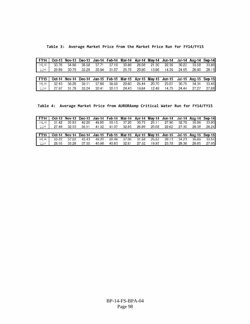
BP-14-FS-BPA-04

Page 98

Table 3: Average Market Price from the Market Price Run for FY14/FY15

Table 4: Average Market Price from AURORAxmp Critical Water Run for FY14/FY15

BP-14-FS-BPA-04

Page 99

Table 5: RevSim Net Revenue Statistics (With PNRR of $0 million)

BP-14-FS-BPA-04

Page 100

Table 6: Risk Modeling Accrual To Cash Adjustments (in $Millions)

A B C D E F

FY 2013 FY 2014 FY 2015

1 Depreciation/Amortization 218.1 224.4 229.3

2 Interest Adjustments (45.9) (45.9) (45.9)

3 ENW Direct Pay Prepaid Expense 12.4 (5.1) (8.0)

4 All Other (see lines 10:18 below) (26.0) (8.7) 8.7

5 Sub Total Lines 1:4 158.5 164.8 184.1

6 Less: Scheduled Federal Debt Amortization (181.6) (159.2) (163.3)

Less: PrePay Principal (8.0) (15.8) (16.6)

7 Less: Revenue/Reserve financing 0.0 0.0 0.0

8 Sub Total Lines 6:8 (189.6) (175.0) (179.8)

9 Accrual to Cash Adjustment (Lines 5 + 8) (31.1) (10.2) 4.2

All Other

10 #N/A 0.0 0.0 0.0

11 Slice Adjustment Cash Lagging out of this year 7.8 0.0 0.0

12 Slice Adjustment Cash Lagging from previous year (11.8) (7.8) 0.0

NORM Slice True Up Lagging out of this year 0.4 1.0 (1.4)

NORM Slice True Up Lagging in from previous year 0.0 (0.4) (1.0)

1 #N/A 0.0 0.0 0.0

2 Terminated contracts & Settlements 0.0 0.0 0.0

3 NTSA Accrual (6.2) 0.0 0.0

4 NTSA Cash Pmt (41.7) 6.2 0.0

5 Other Miscellaneous (0.7) (7.6) 11.1

6 Cash Receipts from FY12 Revenue 26.1 0.0 0.0

7 TOTAL All Other (26.0) (8.7) 8.7

BP-14-FS-BPA-04

Page 101

Table 7: CRAC Annual Thresholds and Caps

[Dollars in Millions]

A B C D E

ANR CRAC CRAC Approx. Maximum

Calculated at Applied Threshold as Threshold as CRAC Recovery

End of Fiscal to Fiscal Measured in Measured in Amount

Year Year ANR PS Reserves (CRAC Cap)*

2013 2014 -$185.5 $0 $300

2014 2015 -$175.3 $0 $300

* The CRAC Cap may be modified by NFB Adjustments

Table 8: DDC Thresholds and Caps

[Dollars in Millions]

A B C D E

ANR DDC DDC Approx. Maximum

Calculated at Applied Threshold as Threshold as DDC Distribution

End of Fiscal to Fiscal Measured in Measured in Amount

Year Year ANR PS Reserves (DDC Cap)

2013 2014 $564.5 $750 $1,000

2014 2015 $574.7 $750 $1,000

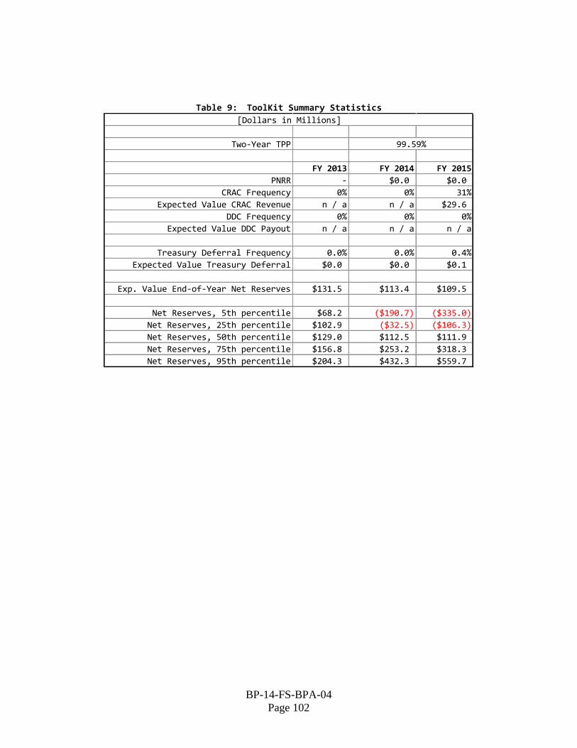
BP-14-FS-BPA-04

Page 102

Table 9: ToolKit Summary Statistics

Two-Year TPP

FY 2013 FY 2014 FY 2015

PNRR - $0.0 $0.0

CRAC Frequency 0% 0% 31%

Expected Value CRAC Revenue n / a n / a $29.6

DDC Frequency 0% 0% 0%

Expected Value DDC Payout n / a n / a n / a

Treasury Deferral Frequency 0.0% 0.0% 0.4%

Expected Value Treasury Deferral $0.0 $0.0 $0.1

Exp. Value End-of-Year Net Reserves $131.5 $113.4 $109.5

Net Reserves, 5th percentile $68.2 ($190.7) ($335.0)

Net Reserves, 25th percentile $102.9 ($32.5) ($106.3)

Net Reserves, 50th percentile $129.0 $112.5 $111.9

Net Reserves, 75th percentile $156.8 $253.2 $318.3

Net Reserves, 95th percentile $204.3 $432.3 $559.7

[Dollars in Millions]

99.59%

BP-14-FS-BPA-04

Page 103

Figure 1: Risk Assessment Information Flow

PN

W H

yd

ro G

en

era

tio

n,

Na

tura

l G

as P

rice

s,

PN

W &

Ca

lifo

rnia

Lo

ad

s,

CG

S O

utp

ut,

BP

A &

PN

W W

ind

Ge

ne

ratio

n,

an

d T

ran

sm

issio

n

& A

ncill

ary

Serv

ice

Exp

en

se

s

Fe

de

ral (

80

WY

) H

yd

ro G

ene

ration

, H

LH

Fe

de

ral H

yd

ro

Shapin

g R

atios, F

edera

l Hydro

Genera

tion A

dju

stm

ents

for

Op

era

ting

Re

se

rve

s

No

n-v

ary

ing

Lo

ad

s &

Re

so

urc

es

Sale

s &

Re

ve

nu

e F

ore

ca

st

for co

ntr

acts

no

t su

bje

ct to

BP

A r

ate

s.

Op

era

tio

na

l

Ris

k

Mo

de

ls

Pro

bab

ilit

y D

istr

ibu

tio

ns

Na

tura

l Ga

s P

rice

s,

PN

W &

Ca

lifo

rnia

Lo

ad

s, P

NW

Win

d G

en

era

tio

n,

CG

S

Ou

tput,

Tra

nsm

issio

n c

apa

city

ava

ilab

ility

, P

NW

, B

C &

Ca

lifo

rnia

(8

0

WY

) H

yd

ro G

en

era

tio

n a

nd

WY

Ind

ice

s

Re

vS

im

(& D

ata

ba

se

)

To

olK

itA

dju

st P

NR

R u

ntil

TP

P >

= 9

5%

Au

rora

PN

W H

LH

& L

LH

Ele

ctr

icity P

rice

s

Pro

babili

ty D

istr

ibution o

f

PS

Op

era

ting

Ne

t R

eve

nu

es

CR

AC

Re

ve

nu

es

,

DD

C C

red

its

,

& T

PP

RA

M R

eve

nu

es,

Exp

en

se

s

RA

M

PN

RR

NO

RM

Pro

babili

ty D

istr

ibutions

for N

on

-Op

era

tin

g

Re

ve

nu

es &

Exp

en

se

s

Pro

bab

ilit

y D

istr

ibu

tio

ns

BP

A L

oa

ds,

CG

S O

utp

ut,

Fe

de

ral

Hyd

ro G

ene

ration

In

dic

es ta

ble

s,

BP

A W

ind

Ge

ne

ratio

n,

Tra

nsm

issio

n a

nd

Ancill

ary

Se

rvic

e E

xp

en

se

s

Su

rplu

s E

ne

rgy

Re

ve

nu

es

,

Ba

lan

cin

g a

nd

Au

gm

en

tatio

n P

ow

er

Pu

rch

as

e E

xp

en

se

s, 4

(h)(

10

)(C

)

Cre

dits

PN

RR

Ch

an

ge

?Yes

No

DO

NE

!

Ste

p 1

: S

tart

ing

In

pu

ts t

o R

isk

An

aly

sis

Ste

p 2

: R

isk

An

aly

sis

Ste

p 3

: T

es

tin

g R

isk

Mit

iga

tio

n t

oo

ls

BP-14-FS-BPA-04

Page 104

Figure 2: AURORAxmp Zonal Topology

BP-14-FS-BPA-04

Page 105

Figure 3: Basis Locations

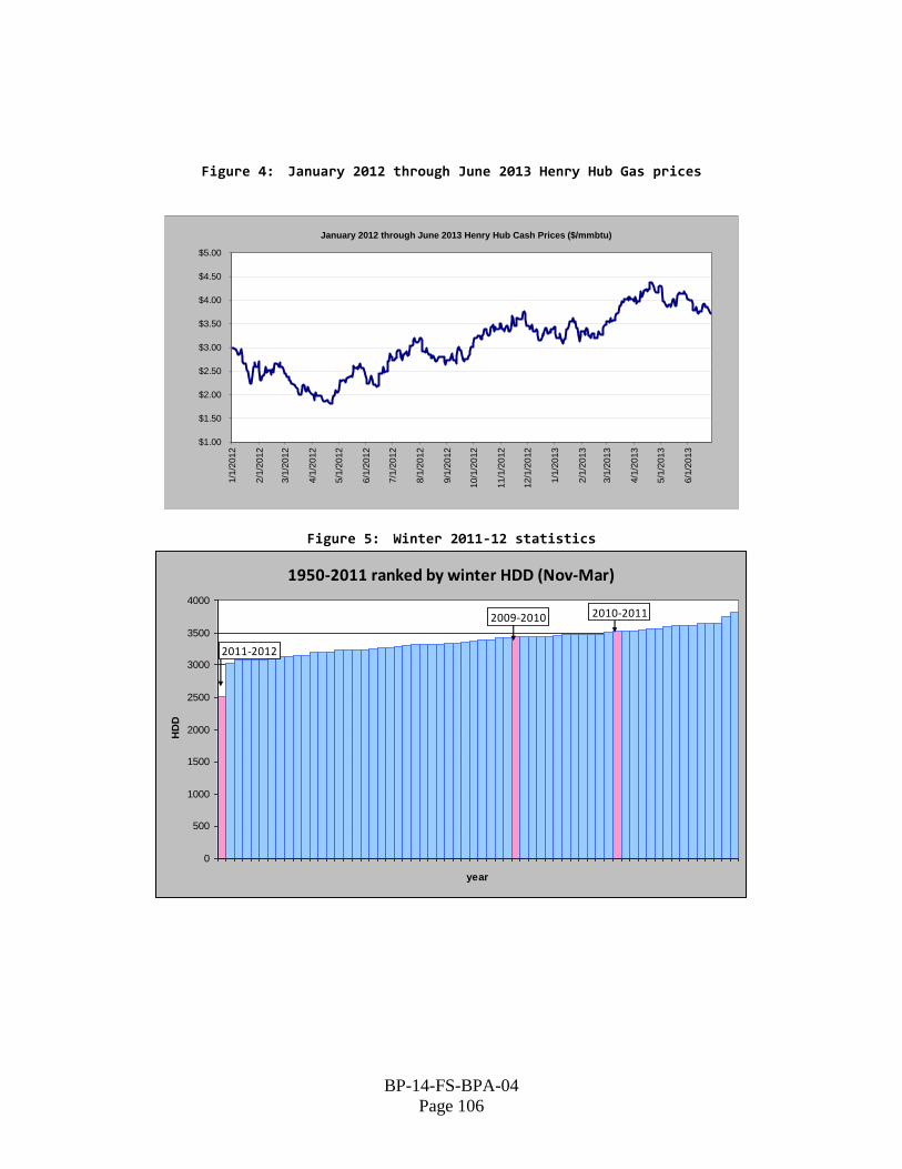
BP-14-FS-BPA-04

Page 106

Figure 4: January 2012 through June 2013 Henry Hub Gas prices

$1.00

$1.50

$2.00

$2.50

$3.00

$3.50

$4.00

$4.50

$5.00

1/1

/201

2

2/1

/201

2

3/1

/201

2

4/1

/201

2

5/1

/201

2

6/1

/201

2

7/1

/201

2

8/1

/201

2

9/1

/201

2

10/1

/20

12

11/1

/20

12

12/1

/20

12

1/1

/201

3

2/1

/201

3

3/1

/201

3

4/1

/201

3

5/1

/201

3

6/1

/201

3

January 2012 through June 2013 Henry Hub Cash Prices ($/mmbtu)

Figure 5: Winter 2011-12 statistics

1950-2011 ranked by winter HDD (Nov-Mar)

0

500

1000

1500

2000

2500

3000

3500

4000

year

HD

D

2011-2012

2009-2010 2010-2011

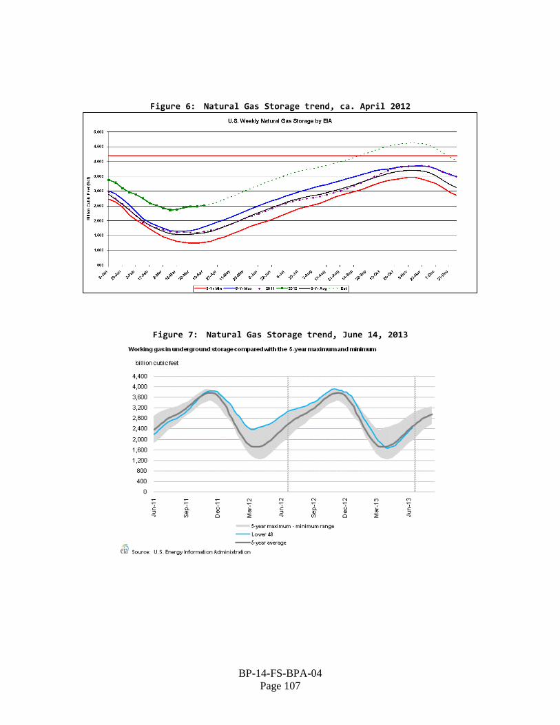
BP-14-FS-BPA-04

Page 107

Figure 6: Natural Gas Storage trend, ca. April 2012

Figure 7: Natural Gas Storage trend, June 14, 2013

BP-14-FS-BPA-04

Page 108

Figure 8: Rig Counts and Production

Figure 9: Historical Coal Prices

BP-14-FS-BPA-04

Page 109

Figure 10: Sumas Imports

BONNEVILLE POW ER ADMINISTRATION DOE/BP-4540 • July 2013