Embed Size (px)
Citation preview

Power System Security Assessment
Application of Learning Algorithms
Christian Andersson
Licentiate ThesisDepartment of Industrial Electrical Engineering
and Automation

Department ofIndustrial Electrical Engineering and AutomationLund UniversityBox 118SE-221 00 LUNDSWEDEN
http://www.iea.lth.se
ISBN 91-88934-39-XCODEN:LUTEDX/(TEIE-1047)/1-90/(2005)
c© Christian Andersson, 2005Printed in Sweden by Media-TryckLund UniversityLund, 2005
ii

School of Technology and SocietyMalmö University

iv
Abstract
The last years blackouts have indicated that the operation and control ofpower systems may need to be improved. Even if a lot of data was available,the operators at different control centers did not take the proper actions intime to prevent the blackouts. This depends partly on the reorganization ofthe control centers after the deregulation and partly on the lack of reliable de-cision support systems when the system is close to instability. Motivated bythese facts, this thesis is focused on applying statistical learning algorithmsfor identifying critical states in power systems. Instead of using a model ofthe power system to estimate the state, measured variables are used as inputdata to the algorithm. The algorithm classifies secure from insecure statesof the power system using the measured variables directly. The algorithm istrained beforehand with data from a model of the power system.
The thesis uses two techniques, principal component analysis (PCA) andsupport vector machines (SVM), in order to classify whether the power sys-tem can withstand an (n−1)-fault during a variety of operational conditions.The result of the classification with PCA is not satisfactory and the techniqueis not appropriate for the classification problem. The result with SVM ismuch more satisfying and the support vectors can be used on-line in order todetermine if the system is moving into a dangerous state, thus the operatorscan be supported at an early stage and proper actions can be taken.
In this thesis it is shown that the scaling of the variables is important forsuccessful results. The measured data includes angle difference, busbar volt-age and line current. Due to different units, such as kV, kA and MW, the datamust be preprocessed to obtain classification results that are satisfactory. Anew technique for finding the most important variables to measure or super-vise is also presented. Guided by the support vectors the variables which haslarge influence on the classification are indicated.
v

vi
Contents
Abstract iv
Preface 1Acknowledgement . . . . . . . . . . . . . . . . . . . . . . 1
1 Introduction 31.1 Previous work . . . . . . . . . . . . . . . . . . . . . . . . . 51.2 Objectives and contributions of the thesis . . . . . . . . . . 61.3 Outline of the thesis . . . . . . . . . . . . . . . . . . . . . . 71.4 Publications . . . . . . . . . . . . . . . . . . . . . . . . . . 7
2 Power system control 92.1 Power system stability . . . . . . . . . . . . . . . . . . . . 92.2 Power system operation . . . . . . . . . . . . . . . . . . . . 12
3 Data set 153.1 Data set structure . . . . . . . . . . . . . . . . . . . . . . . 153.2 The NORDEL power system . . . . . . . . . . . . . . . . . 163.3 NORDIC32 . . . . . . . . . . . . . . . . . . . . . . . . . . 183.4 The 2k factorial design . . . . . . . . . . . . . . . . . . . . 213.5 Dimension criterion . . . . . . . . . . . . . . . . . . . . . . 223.6 Training set . . . . . . . . . . . . . . . . . . . . . . . . . . 233.7 Classification set . . . . . . . . . . . . . . . . . . . . . . . 243.8 Conclusions . . . . . . . . . . . . . . . . . . . . . . . . . . 26
4 Principal component analysis 274.1 Principal component analysis . . . . . . . . . . . . . . . . . 27
vii

4.2 Number of principal components . . . . . . . . . . . . . . . 294.3 Scaling . . . . . . . . . . . . . . . . . . . . . . . . . . . . 30
4.3.1 Scaling to keep the physical properties . . . . . . . . 314.4 Classifying power system stability with PCA . . . . . . . . 324.5 Conclusions . . . . . . . . . . . . . . . . . . . . . . . . . . 32
5 Support vector machines 375.1 Linear support vector machines . . . . . . . . . . . . . . . . 37
5.1.1 Maximal margin optimization . . . . . . . . . . . . 385.1.2 Soft margin optimization . . . . . . . . . . . . . . . 40
5.2 Scaling . . . . . . . . . . . . . . . . . . . . . . . . . . . . 435.2.1 Scaling to keep the physical properties . . . . . . . . 435.2.2 Scaling of unit stator current after capacity . . . . . 445.2.3 Variables . . . . . . . . . . . . . . . . . . . . . . . 44
5.3 SVM training . . . . . . . . . . . . . . . . . . . . . . . . . 455.4 Classifying with a hyperplane . . . . . . . . . . . . . . . . 475.5 Reducing variable sets . . . . . . . . . . . . . . . . . . . . 51
5.5.1 Different variable setup . . . . . . . . . . . . . . . . 525.6 Implementation . . . . . . . . . . . . . . . . . . . . . . . . 725.7 Results . . . . . . . . . . . . . . . . . . . . . . . . . . . . . 735.8 Conclusions . . . . . . . . . . . . . . . . . . . . . . . . . . 74
6 Conclusions 756.1 Summary of the results . . . . . . . . . . . . . . . . . . . . 756.2 Future work . . . . . . . . . . . . . . . . . . . . . . . . . . 76
Bibliography 77
viii

Preface
During the final year of my B.Sc. studies in 2001 I was introduced to thechallenges related to planning and operation of power system by my currentPhD-advisor Bo Eliasson. I was studying computer and electrical engineer-ing at Campus Norrköping, Linköping Institute of Technology. When plan-ning my undergraduate project I contacted Daniel Karlsson at ABB Tech-nology Products and came to work with wide area protection system againstvoltage collapse. The project was supervised by Bo Eliasson at Malmö Uni-versity. It was during my undergraduate project I became aware of the specialproblems with multi input multi output system (MIMO), many of the powersystems today are probably the largest MIMO system ever built by mankind.In the summer of 2002 I was appointed a PhD position at Malmö Universityand was accepted to the post-graduate study program at Lund Institute ofTechnology.
1

2
Acknowledgement
First of all, I would like to thank my supervisors, Bo Eliasson for introducingme to the interesting problems in power system control and for his supportand advice. Gustaf Olsson for accepting me as a Ph.D. student at his depart-ment and for his encouragement and optimism. Olof Samuelsson who leadsthe electric power system automation research group at IEA, the guidance,support and comments on my work have been very important.
I am also very grateful to Sture Lindahl for support and many interestingdiscussions. Jan Erik Solem for introducing me to pattern recognition. Theconstant guidance, support and unlimited help has helped me a lot, this thesishad not been made without you. Lars Lindgren for help with the ARISTOsimulator and all the discussions about power systems we have had, I havelearned a lot from you.
I would like to thank the graduate students and researchers of the Indus-trial Electrical Engineering and Automation at Lund Institute of Technologyand Applied Mathematics Group at Malmö University, especially to: ErikAlpkvist, Yuanji Cheng, Pär Hammarstedt, Adam Karlsson, Niels Chris-tian Overgard, Fredrik Nyberg and Markus Persson for providing a creative,happy and sometimes confused atmosphere.
Furthermore, I would like to thank Gun Cervin and Yvonne Olsson atKranenbiblioteket, Malmö University for their excellent service. I am alsograteful to Jan Erik Solem, Olof Samuelsson and Christian Rosén for proof-reading this thesis.
I would like to thank my family and friends, especially my two youngersisters for their patience, even though I am always teasing them, (Josefin, jagvet att jag är ditt elände). Finally, Cissi, you´re the best.
Malmö, August 21, 2005Christian Andersson

Chapter 1
Introduction
In August and September 2003 three major blackouts occurred in N.E. NorthAmerica, S. Scandinavia and Italy. About 110 million people were affectedby these events. The interruption time ranged from a couple of hours to days.The reason why these blackouts occurred were partly due to the lack of sup-portive applications when the system is close to instability. If the powersystem is close to the stability limit, actions must be taken by system opera-tors to counteract a prospective blackout. Today a large problem for systemoperators is to identify critical states since there are thousands of parameterswhich describe and affect the state.
The deregulation of the power markets has contributed to the fact that thepower systems today are frequently operated close to stability limit. This isdue to a larger focus on economical profits instead of system security andpreventive maintenance.
The last three years the consumption of electrical power in the world hasincreased with 3 %, each year. That corresponds to investments of 60 bil-lion USD each year in production and transmission equipment to match theincreased consumption. If the trend continues actions must be taken to main-tain system stability.
The latest blackouts and deregulated power markets contribute to an in-creased requirement of Wide Area Protection Schemes (WAPS). The WAPSwill make it possible to change the operation criteria from: ”The power sys-tem should withstand the most severe credible contingency” to ”The powersystem should withstand the most severe credible contingency, followed byprotective actions from the WAPS.”
3

4 Chapter 1. Introduction
In this thesis classification of power system stability defines a method toseparate secure from insecure states in power systems. Due to the complex-ity of power system with the large amount of states and the large amountof variables that describe the states it is difficult to estimate the stabilityof power systems. The purpose with this thesis is to examine methods forclassifying power system stability with techniques from pattern recognition.The methods use the measured variables, such as busbar voltage, line currentand active current of generators, of the power system to decide the stabilityof the power system. The classification algorithm which is developed withtechniques for pattern recognition is trained from a data base. The data base,denoted training set, consists of measurements from different states of thepower system. With the algorithm it should be able to estimate the stabilityof all the states of the power system may operate in. Therefore it is importantthat the training set properly describes the variations of the power system. Itmust be considered that if the training set does not show enough variability,the algorithm is useless. A properly trained algorithm can separate the train-ing set into two parts. One consists of stable states and the other of unstablestates. The algorithm can then be used to decide the class of unknown states.
This should be used as a supportive tool for the system operators to fasterform an opinion of the actual state of the power system. This could alsomake it easier to decide what needs to be done by the system operators toavoid a blackout. Compared with the WAPS the classification method shouldprompt system operators at control centers to take preventive actions beforethe WAPS will act.
The work with this thesis started with the development of the training set.Thereafter Principal Component Analysis (PCA) was applied to the classifi-cation problem. The result with PCA was not satisfactory. Therefore Sup-port Vector Machines (SVM) was used to find a solution of the classificationproblem. SVM calculates a hyperplane that separates a data set from theirpredefined classes. The SVM method is more adaptable to the classificationproblem in this thesis than PCA and the result is much more satisfying.

1.1. Previous work 5
1.1 Previous work
This thesis deals with the problem of classification of power system stabil-ity. An overview of power system stability and design can be found in thestandard textbooks [13] and [22]. In [23] the CIGRE Study Committee 38and the IEEE Power System Dynamic Performance Committee gives a back-ground and overview of power system stability with the focus on definitionand classification. A nice introduction to power system voltage stability canbe found in [34], which has a detailed description of reactive power com-pensation and control. These books and reports gives a good overview andbackground to power system design and control.
Previous work on power systems stability has been focused on identifica-tion and finding methods to prevent instability. In [6] and [26] the problemwith voltage instability is analyzed, these two theses are a part of the previ-ous work that is the inspiration to this thesis. Another work that has beena great inspiration to this thesis is the research by Louis Wehenkel which issummarized in [39]. Wehenkel uses the same approach to the stability prob-lem as in this thesis but he uses decision trees instead of principal componentanalysis and support vector machines.
The knowledge about separation with a hyperplane has been known forquite long time, but the calculation of the hyperplane has caused problems.In 1992 Support Vector Machines (SVM) was introduced by Vapnik, see[37]. It is described in detail in [36]. The SVM calculate a hyperplane withthe maximal margin between the two classes. This is done using a globaloptimization problem on quadratic form, which can easily be solved.
The last years SVM has been used to find methods to solve many classi-fication and regression problems. In [16] and [31], SVM has been appliedto face detection with successful results. Text categorization has also beenimproved with SVM, see [18]. In [19], windows are detected from picturesof city scenes. The author has found one publication which deals with clas-sification of power system stability using SVM, see [30]. In the article clas-sification of power system stability is made with nonlinear SVM and neuralnetworks. The data set which is used has an impressive size, and the resultof the classification is very successful.

6 Chapter 1. Introduction
1.2 Objectives and contributions of the thesis
The main objective of this thesis is to investigate if it is possible to use sta-tistical learning algorithms for classification of power system stability. Theobjectives of this thesis are listed below.
• Find a method which makes it possible to classify the stability of apower system from measurements without calculating the state of thepower system.
• Adjust the classification method for the application to power systemstability.
• Investigate if the classification method can be implemented in real-time so that operation of power systems can be simplified and alsoimproved.
People with different background should be able to read and comprehend thethesis. This means that some readers will consider some parts of the thesis asobvious. However, if the reader is not oriented in power system fundamentalsan introduction can be found in [13] and [22]. The main contributions of thethesis are listed below.
• The power system stability is classified with a hyperplane, which iscalculated with Support Vector Machines (SVM). The SVM offers aclassification method with the largest distance between the two classes.
• Methods to improve the classification by using an appropriate scalingalgorithm. Investigations of which variables should be used to repre-sent the power system in order to improve the classification result.
• Methods to reduce the number of measured variables are introduced.Thus the classification can be made by a subset of the measurable vari-ables without losing the number of correct classifications.
• Method for handling the difficulties of classification with statisticallearning algorithm with a mixture of continuous and binary variables.
1.3. Outline of the thesis 7
1.3 Outline of the thesis
The thesis consists of two parts, the design of the data set and two differentmethods applied to the classification problem.
In the first part, Chapter 2, an overview of power system stability and op-eration is given. Furthermore, the contribution of this thesis to the power sta-bility problem is described. In Chapter 3, a short summary of the NORDELpower system and the operation rules is given. Thereafter, an introduction todesign of experiments with factorial design is given. Finally, the design ofthe data set is described.
The second part consists of Chapter 4 and Chapter 5. In Chapter 4 theunsupervised learning method principal component analysis is applied to theclassification problem and in Chapter 5 the supervised learning method ofcalculating a hyperplane with support vector machines is applied to the clas-sification problem. Chapter 6 summarizes the results and suggests futurework.
1.4 Publications
The thesis is based on the following publications:
[1] C. Andersson, J E. Solem and B. Eliasson. Classification of powersystem stability using support vector machines. In IEEE Power En-gineering Society General Meeting. San Francisco, California, USA,June 12-16. 2005.
[2] L. Lindgren, B. Eliasson and C. Andersson. Damping of power systemoscillations using phasor measurement units and braking resistors. InIFAC proceedings of reglermöte. Gothenburg, Sweden, May 26-27.2004.
[3] B. Eliasson and C. Andersson. New selective control strategy of powersystem properties. In IEEE Power Engineering Society General Meet-ing. Toronto, Ontario, Canada, July 13-17. 2003.
[4] B. Eliasson and C. Andersson. New selective control strategy of thevoltage collapse problem. In CIRED 17th International Conferenceon Electricity Distribution. Barcelona, Spain, May 12-15. 2003.

8 Chapter 1. Introduction

Chapter 2
Power system control
This chapter consists of a brief overview of power system operation and thesecurity limits that are taken to maintain system stability in stressed situa-tions.
2.1 Power system stability
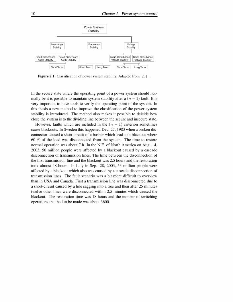
The stability of power systems is defined as: "The ability of an electric powersystem, for a given initial operating condition, to regain a state of operatingequilibrium after being subjected to a physical disturbance, with most sys-tem variables bounded so that practically the entire system remains intact",[23]. This means that some faults should not cause any instability problems.Figure 2.1 shows different stability states. Due to the complexity of powersystems, the different instabilities affect each other. A blackout scenariooften starts with a single stability problem but after the initial phase otherinstability problems may occur. Therefore the actions in order to prevent ablackout in stressed situations may be different. For a detailed description ofthe different stability scenarios see [23]. Due to mainly economical factorsthere is a limit of which faults the system should withstand and remain instability.
The synchronous NORDEL system (Sweden, Norway, Finland and Sealand)is dimensioned to fulfill (n−1) criterion, which means that the system shouldwithstand a single fault, e.g. short circuit of busbar or disconnection of nu-clear unit, see [1]. In Figure 2.2 the different operative states are illustratedand how the power systems operation state can change due to a disturbance.
9
10 Chapter 2. Power system control
Power System Stability
Rotor Angle Stability
Frequency Stability
Voltage Stability
Small-Disturbance Angle Stability
Small-Disturbance Angle Stability
Large-Disturbance Voltage Stability
Small-Disturbance Voltage Stability
Short Term Short Term Long TermShort Term Long Term
Figure 2.1: Classification of power system stability. Adapted from [23] .
In the secure state where the operating point of a power system should nor-mally be it is possible to maintain system stability after a (n − 1) fault. It isvery important to have tools to verify the operating point of the system. Inthis thesis a new method to improve the classification of the power systemstability is introduced. The method also makes it possible to deicide howclose the system is to the dividing line between the secure and insecure state.
However, faults which are included in the (n − 1) criterion sometimescause blackouts. In Sweden this happened Dec. 27, 1983 when a broken dis-connector caused a short circuit of a busbar which lead to a blackout where60 % of the load was disconnected from the system. The time to restorenormal operation was about 7 h. In the N.E. of North America on Aug. 14,2003, 50 million people were affected by a blackout caused by a cascadedisconnection of transmission lines. The time between the disconnection ofthe first transmission line and the blackout was 2,5 hours and the restorationtook almost 48 hours. In Italy in Sep. 28, 2003, 53 million people wereaffected by a blackout which also was caused by a cascade disconnection oftransmission lines. The fault scenario was a bit more difficult to overviewthan in USA and Canada. First a transmission line was disconnected due toa short-circuit caused by a line sagging into a tree and then after 25 minutestwelve other lines were disconnected within 2,5 minutes which caused theblackout. The restoration time was 18 hours and the number of switchingoperations that had to be made was about 3600.

2.1. Power system stability 11
SE
CU
RE
INS
EC
UR
EA
SE
CU
RE
PREVENTIVE STATE
NORMAL
Control and / or protective actions
Foreseen or unforeseen disturbance
Maximize economy and minimize the effect of uncertain contingencies
RESTORATIVE ALERT
IN EXTREMIS EMERGENCY
Resynchronization Load pickup
Tradeoff of preventive vs corrective control
Partial or total service interruption
Overloads Undervoltages Underfrequency... Instabilities
Preventive control
Emergency control (corrective)
Protections
Split Load shedding
Figure 2.2: The operating states and transitions for power systems. Adaptedfrom [12] .

12 Chapter 2. Power system control
In Figure 2.2 the state during abnormal situations are described with theinsecure and asecure states. If a power systems operating point moves fromthe secure to the insecure state, actions must be taken by system operatorsto return to the secure state. By the three blackouts in Sweden, N.E. NorthAmerica and Italy, it is shown that the preventive time interval can be be-tween 50 seconds to 2,5 hours. From a system operation point of view it ispossible to take actions before entering the insecure state. This thesis hasfocus on supportive information, before entering the insecure area. In theasecure state, only automatic actions and control are realistic.
Blackouts have occurred and will happen in the future, but the objectivefrom the power industry is to increase the time between the blackouts andalso minimize the number of people which are affected. By e.g. support-ive applications for the operators based on new technology, the preventionagainst blackouts can be improved. By increased automation the imbalancesbetween production and consumption can be quickly alleviated. Also theblack-start capability after a blackout can be improved.
2.2 Power system operation
In power system control today the operating point is validated by a stateestimator and tools to calculate system collapse limit. There are differentsoftware tools developed for this. In [35] the experience with implementinga voltage security assessment tool at B.C. Hydro, Burnaby, Canada is de-scribed. In Sweden today SPICA is used to calculate the voltage collapselimits. SPICA is developed by Swedish National Grid (Svenska Kraftnat)and uses an estimate to calculate the voltage collapse limits by load-flowcalculations. Mainly by increasing the load in sensitive parts of the systemand exposing them for a selection of (n − 1) faults. The predictor proposeschanges in such as,
• Transfer limits
• Increased production
• Decreased export by HVDC,
if the estimated operating point does not fulfill the (n − 1) condition.The limitations with the state estimators are that they use a model of the
power system. There is always a difference between the model and the real

2.2. Power system operation 13
system. It is also common to use load-flow calculations. In a load-flowcalculation the dynamic part of the elements in the model are neglected e.g.load dynamic and also often voltage regulators and current limiters. Theload-flow solver calculates an operating point where there is balance in activeand reactive power. There is a difference between load-flow calculation anddynamic simulation. When the operating condition changes, e.g. by a short-circuit of a busbar, the load-flow solver calculates the operating point afterclearance of the fault. The dynamic simulation also analyzes the effect bye.g. automatic equipment. Hence the operating point after the transientsare settled will be different compared with a load-flow calculation. Thiscan result in that the operating point calculated by load-flow is stable but ifthe scenario is analyzed by dynamic simulation a blackout can occur in thetransient phase.
In this thesis, dynamic simulations are used to develop classification meth-ods which are used to estimate the bound between the secure and the insecurestate, see Figure 2.2. Instead of using a traditional state estimator, statisticallearning algorithms are used to calculate an algorithm which uses measuredvariables, e.g. busbar voltage, angle difference and line current to classifythe stability.

14 Chapter 2. Power system control

Chapter 3
Data set
In this chapter the data set for verifying the statistical learning algorithmsapplied on classification of power system stability is described. With thealgorithm is should be possible to estimate the class for all states in the powersystem. It is therefore important that data set properly describe the variationsof the system. It must be considered that if the data set does not show enoughvariability, the SVM cannot be successfully applied.
To create a function for classification with a learning machine with the bestconditions, the space of operation should be covered by the data set. In e.g.chemical processes, design of experiments are used to cover the operationspace with a limited number of experiments, for details see [10].
The data set used to verify the classification algorithms has not been de-signed with experimental design since it would become very large. The timeit takes to prepare the simulator and collect the data are not covered in thisproject. Instead, the knowledge about the daily operation of the NORDELsystem and the problems that has caused stressed operation situations hasbeen taken into account to create the data set.
3.1 Data set structure
In this thesis the data set is organized as a matrix, see Table 3.1. A row in thematrix, denoted with an example, is the state of the power system contain-ing the measured variables. The label vector consists of the binary code
for each example. If the example sustains the dimension criterion (n − 1),see Section 3.5, has the binary code +1, otherwise -1.
15

16 Chapter 3. Data set
Table 3.1: Description of how the data set is organized, the label vector con-sists of the binary code to the corresponding examples.
VariablesExample 1
...Example l
Label+1...
-1
3.2 The NORDEL power system
In this presentation of NORDEL, Iceland and Jutland (Denmark) are ex-cluded, for details see Figure 3.1. The synchronous system consisting ofFinland, Norway, Sealand (Denmark) and Sweden is presented. The installedcapacity was 93 GW on Dec. 31, 2003, the maximum load was 58 GW, mea-sured on Jan. 15, 2003. In Table 3.2 the distribution of the installed capacityper country is listed. The information about the NORDEL power systempublished here is obtained from [4].
In Sweden, a large amount of hydro power is located in the northern partand nuclear power is located in the southern part. Because of a larger load de-mand in the south of Sweden the power flow normally is from north to south.The latest blackouts in Sweden (1983 and 2003) occurred because of reducedcapacity in the transmission system, see [3] and [7]. The NORDEL systemdata is not used here, but instead a simplified model called NORDIC32 isused. This simplified model should be compared with the NORDEL powersystem in order to give guidelines for the design of the data set. To classifythe stability of a power system, traditionally bus voltage and system fre-quency have been used. In Sweden the transfer of active power on roughly10 selected transmission lines are used as guidance for the system stabil-ity. The transmission system is divided into 4 cut-sets, called Snitt 1− 4.Snitt 4 measures the sum of active power of the 5 transmission lines thatconnect the south of Sweden with the rest of the system, see Figure 3.1. Op-eration aims at keeping the transport of active power through Snitt 4 belowa certain threshold to retain system stability from the most severe crediblecontingency.

3.2. The NORDEL power system 17
Figure 3.1: The NORDEL main grid, 2000, The cut-sets, Snitt 1 to 4, aremarked.

18 Chapter 3. Data set
Table 3.2: Installed capacity in NORDEL on 31 Dec. 2003, MW.Denmark Finland Norway Sweden
Hydro power 11 2 978 27 676 16 143Nuclear power - 2 640 - 9 441Other thermal power 9 704 11 225 305 7 378Renewable power 3 115 50 100 399
3.3 NORDIC32
The NORDIC32 (N32) system is used for the study [5]. It is an equivalent orsimplified model of a transmission system with similarities to the Swedishpower system, see Figure 3.2. The generation consists of approximately45 % nuclear, 45 % hydro and 10 % other thermal power. The installedcapacity is 17 GW, see Table 3.3. The system has 32 substations, 35 units,50 branches and the number of measurable variables are 653. To adjust thespinning reserve and speed droop the relation between N32 and NORDELare settled to approximately 1:4.
In order to produce the data set, the platform described below was used.Since 1996 the simulator ARISTO (Advanced Real-time Interactive Sim-ulator for Training and Operation) has been used for operator training atSwedish National Grid (Svenska Kraftnät). The simulator has unique fea-tures for stability analysis in real time [9]. Not only that, the simulationproves to be extremely robust during abnormal operating conditions. UsingARISTO the operators obtain a better understanding of the phenomena thatmay cause limitations and problems to power transmission and distributionsystems.
The load models in ARISTO cover the load dynamics (short and longterm) and load characteristics (voltage and frequency dependence) very well.Transmission lines are represented with pi-equivalents. The generation unitsare represented by synchronous generators and turbine governors, either ther-mal or hydro. The protection equipment implemented in ARISTO are
• Line distance protection
• Line over-current protection

3.3. NORDIC32 19
Table 3.3: Installed capacity in NORDIC32, MW.Finland Norway Sweden
Hydro power 4 605 1 520 4 740Nuclear power - - 4950Other thermal power - - 1 080
• Unit over/under frequency protection
• Unit over/under voltage protection
and the automatic equipment
• Load disconnection due to under-frequency
• Shunt capacitor/reactor connect/disconnect due to under/over voltage.
The detailed representation of power system models in ARISTO results ina more realistic data set than if a simple load-flow solver had been used.The difference between load-flow calculations and dynamic simulations isthat load-flow solvers calculate an operation point for the given conditions,whereas dynamic simulations calculate a time-simulation where the oper-ating point is calculated for each time step. The advantage with dynamicsimulations is that it is possible to analyze the influence of automatic protec-tion, control equipment and dynamic models on the power system. In thisstudy a three-phase short-circuit on a busbar is analyzed. With the dynamicsimulation it is possible to take into account what has happened during thetransients. With a load-flow solver it is only possible to analyze if thereis balance in active and reactive power after the disconnection of the fault.Therefore, the data set is more realistic with the dynamic simulation.
The main additives to the simulator consist of a multi-user communicationlink between the Application Programmable Interface (API) of ARISTO andMatlab/Simulink. This function is used to collect the data set.

20 Chapter 3. Data set
Figure 3.2: The NORDIC32 system.

3.4. The 2k factorial design 21
3.4 The 2k factorial design
Factorial designs are often used in designs of experiments. The purposeis to cover most of the variation in the process with a limited number ofexperiments, see [10] and [29]. The elements in the design consist of factorsand response. Response is the output of the process. Factors are the elementsin the process that influence the output. The factors can be both controllableand uncontrollable.
For classification of power system stability the label of the example is de-cided according to the Nordel grid planning rules for the Nordic transmissionsystem, for details see [1]. Therefore the factorial design is applied with thefollowing factors
• Production
• Transmission capability
• Consumption
and responses
• Bus voltages
• Angle differences
• Line current
• System frequency
• Load disconnection from system protection.
The purpose with factorial design is to define a high and a low level forevery factor. In 23 design the factors form a cube where the examples shallbe chosen from the corners of the cube, see Figure 3.3. If the factorial designis applied to the N32 system the number of simulations will be very large.Taken into account that the number of units are 35, branches 50 and loads59 the simulation time will be very long. Approximations can of course bemade. Using only nuclear power, a data set could be designed with factorialdesign. The number of substations with nuclear power are 5, thus the numberof examples in the data set would be 32. The problem is to design a data setthat also has a variation in production of hydro units, power flow, and load,

22 Chapter 3. Data set
Figure 3.3: Illustration of a factorial 23 design.
with a limited number of examples. Therefore factorial design is not usedto design the data set. Instead, knowledge from operation of the NORDELsystem with already known limits has been used in the design of the data set.
3.5 Dimension criterion
According to Nordic grid instructions, the Nordel system must fulfill the(n− 1) criterion, see [1] and [2]. An example is considered acceptable if thepower system can withstand any single failure. The system has withstood acontingency if:
• There is no load shedding, due to under frequency.
• The final post-fault voltage profile is acceptable.
• The final post-fault frequency is acceptable.
The contingencies are e.g. disconnection or short-circuit of a line, load,shunt or busbar. After fault clearance the voltage profile is acceptable ifall except one busbar are within 10 % of the normal operating voltage. Thesystem frequency is accepted if it does not drop below 49.0 and exceeds 49.5Hz after 30 seconds. The upper level demand on the frequency is 52.0 Hzand it must be lower than 50.6 Hz after 30 seconds.

3.6. Training set 23
To verify the (n−1) criterion for the examples, a three-phase short-circuitat all busbars, one at a time, is used to decide the binary code according tothe rules above. This is done for each of the training examples. The faultis cleared 80 ms after the fault appeared, see [13]. In practice this is donein ARISTO by first applying the fault to the example, then after 80 ms thefault is cleared, finally after 240 s it is considered that the transients areapproximately settled and the simulation is stopped. The binary code is thendecided for the example.
Because N32 is an equivalent, with reduced topology, the (n−1) criterionis not fulfilled by most of the examples in the data set. The data set is splitinto three classes:
1. Examples where a single fault leads to system black-out.
2. Examples where a single fault leads to black-out in two or three sub-stations.
3. Examples which fulfill the (n − 1) criterion.
Therefore a method shall be developed to identify class 1 and separateclass 1 from class 2 and 3.
3.6 Training set
As training data, four base generation patterns are used.
• NN, all nuclear power at maximum production.
• NO, all nuclear power at maximum production on the west coast, nonuclear power on the east coast.
• ON, all nuclear power at maximum production on the east coast, nonuclear power on the west coast.
• OO, no nuclear power on-line.
The first step is to find the minimum load level for the four generation pat-terns, by scaling the active power part of the load on a common system base.To create balance in the system at the minimum level the production of hy-dro power is corrected. As little hydro power as possible should be used to

24 Chapter 3. Data set
create balance in the minimum case. In order to achieve training data withthe characteristics of the NORDEL power system the following dimensioncriteria are used for all examples.
• The system frequency is within 50 ± 0,01 Hz.
• The voltage profile is adjusted according to [24], where the normal op-eration voltage on the 400 kV level is 400-415 kV, with the minimumaccepted voltage 395 kV and the maximum accepted voltage 420 kV.
• The spinning reserve in the system is 750 MW, divided on three hydropower units. It corresponds to the largest unit in N32.
• The ratio between N32 and NORDEL is approximately 1:4. Taken thisinto account the speed droop is tuned to about 1500 MW/Hz for allmodels. The Nordel system (Sweden, Finland, Norway and Sealand)it is 6000 MW/Hz, see [2].
When the minimum load level is achieved, a new model is created by increas-ing the load level by 5 % increments from the base load profile. Spinningreserve and the speed droop is tuned so that all models have similar charac-teristic. For the 4 generation patterns the load level is increased with 5 %until the maximum load level is identified. The total number of models inthe training data is 30, with a consumption between 3 280 and 13 570 MW.This is done in order to extend the generation/transmission patterns as muchas possible with a limited number of training models. The generation andconsumption of reactive and active power for the 30 examples in the trainingset are listed in Table 3.4. The label for the examples are also listed here.Table 3.4 shows that the increased consumption for the three different basepatterns, NN, NO, ON, does not imply a more stressed state.
3.7 Classification set
The classification algorithm is developed with a training set and validatedwith a classification set. To show the performance of the algorithm. Theclassification set consists of 16 examples. These are created from 16 of theexamples in the training data that have been manipulated e.g. increased loadfactor and disconnection of single line or unit. Thus, an example which

3.7. Classification set 25
Table 3.4: The system generation and consumption for the examples in thetraining set, MW and MVar.
Name PGeneration Pload QGeneration Qload Label
NN1 7 489 7 329 1 550 3 359 -1NN2 8 869 8 752 975 3 359 1NN3 9 968 9 846 1 244 3 359 1NN4 10 545 10 392 907 3 359 -1NN5 11 136 10 940 1 019 3 359 -1NN6 11 707 11 487 970 3 359 1NN7 12 463 12 034 2 386 3 359 -1NN8 12 948 12 581 1 640 3 359 1NN9 13 545 13 128 2 019 3 359 1NN10 14 075 13 566 2 832 3 359 -1NO1 4 541 4 376 1 126 3 359 1NO2 5 667 5 470 857 3 359 1NO3 6 826 6 564 998 3 359 1NO4 7 418 7 111 1 199 3 359 -1NO5 8 021 7 658 1 440 3 359 -1NO6 8 630 8 205 1 581 3 359 -1NO7 9 266 8 752 2 408 3 359 -1ON1 4 468 4 375 915 3 359 1ON2 5 556 5 470 873 3 359 1ON3 6 674 6 564 798 3 359 1ON4 7 243 7 111 780 3 359 -1ON5 7 819 7 657 777 3 359 -1ON6 8 405 8 205 908 3 359 1ON7 8 998 8 752 1 041 3 359 1ON8 9 608 9 299 1 382 3 359 1ON9 10 203 9 846 1 580 3 359 1ON10 10 835 10 393 2 262 3 359 1OO1 3 428 3 282 760 3 359 -1OO2 4 639 4 376 1 075 3 359 -1OO3 5 905 5 470 2 254 3 359 -1

26 Chapter 3. Data set
fulfills the criterion in the training set is manipulated so that it does not fulfillthe criterion in the classification set. The binary code for the examples isdecided with the same criterion as for the training set.
3.8 Conclusions
In this chapter the data set that will be used to verify the classification meth-ods in Chapter 4 and 5 described. The methods to design the different ex-amples and the dimension criterion for deciding the binary code are pre-sented. The detailed protection equipment in ARISTO, adjustment of spin-ning reserve, speed-droop, transient analysis and comparison to Nordel gridinstructions improves the quality of the data set. The ARISTO simulator isused instead of a normal load flow solver, which improves the quality.

Chapter 4
Principal component analysis
In this chapter an introduction to Principal Component Analysis (PCA) willbe given. PCA is one of the most popular unsupervised learning methods.The main reason is that the method reduces the dimension of the data set.With PCA the variables in the data set are projected to a lower dimensionalspace described by the principal components, see [14], [15] and [20]. Thusthe characteristics of a multivariate process can hopefully be shown in lowerdimensions. The projection of the data set on the principal components cangive an unexpected relationship between the process and the variables.
Today in supervision and control of power systems the main problemsare not to measure and collect data. The Supervisory Control And DataAcquisition (SCADA) system gives this possibility. The main problem is toidentify examples which do not fulfill the (n − 1) criterion. Furthermore, itmight not be necessary to use all measured variables from the power systemfor the identification. Which variables that can be reduced is an importantquestion to investigate.
4.1 Principal component analysis
PCA was introduced by Pearson in 1901 [32]. With PCA the dimension ofthe data set is reduced from Rd to Rn, where n ≤ d. The principal com-ponents are orthogonal in Rn. The principal components are the directionsin the data set with the highest variance, see Figure 4.1. An introduction tohow the principal components are calculated will be given below.
27

28 Chapter 4. Principal component analysis
**
***
**
**
**
***
*
*
*
*
*
**
* *
W1
Figure 4.1: The first linear principal component of a data set. The line mini-mizes the total squared distance from each point to its orthogonalprojection onto the line.
Denote the data setXl×d ,
where X is the data set stored as l examples with d variables. Let x =(x1, . . . , xd) be the mean value for all variables and,
X = [x1 − x1, . . . ,xd − xd] ,
where xi, i = 1, . . . , d are the columns in X.
The covariance matrix of X, see [25], is
Σ =1
l − 1X>X .
The principal components of X can be calculated by solving the eigenvalueproblem,
ΣΦ = ΛΦ ,

4.2. Number of principal components 29
where Φ is an orthogonal matrix and Λ is a diagonal matrix containing theeigenvalues. The eigenvectors to X>X, Φ can also be calculated with Sin-gular Value Decomposition (SVD) of X, as
X = USV>,
where Ul×l and Vd×d are orthogonal matrices and Sl×d is a diagonal matrixcontaining the singular values. The first principal component, the direction inthe data set with largest variance captured with a linear function, is the eigen-vector with the largest corresponding singular value. The SVD-factorizationis usually defined with the singular values in descending order.
In [15] and [11] the calculation of principal components are denoted with
X = TP + E , (4.1)
where Tl×n are called score vectors, Pd×n are called loading vectors, n isthe number of principal components and E is the residual or variance in thedata set not described by the principal components. T and P are calculatedas,
I = {i1, i2, . . . , id}J = {i1, i2, . . . , in}P = V>{I, J}T = XP> ,
where V>{I, J} are all the rows and the n first columns of V>.
4.2 Number of principal components
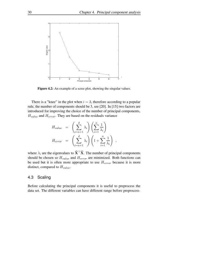
How to choose the correct number of principal components is something thatis difficult to answer. There are some values that can be calculated to guidethe decision. If too many principal components are used the dimension ofthe data set is not reduced enough. On the other hand, if too few principalcomponents are used, the residuals will be too large. For PCA the numberof components is usually chosen by guidance from the eigenvalues. In Fig-ure 4.2 the singular values of X are shown, it is sometimes denoted withscree plot [20].
30 Chapter 4. Principal component analysis
0 1 2 3 4 5 6 70
1
2
3
4
Principal component
Sin
gula
r val
ue
i
Figure 4.2: An example of a scree plot, showing the singular values.
There is a ”knee” in the plot when i = 3, therefore according to a popularrule, the number of components should be 3, see [20]. In [15] two factors areintroduced for improving the choice of the number of principal components,Hvalue and Herror. They are based on the residuals variance
Hvalue =
(d∑
i=n+1
λi
)(n∑
i=1
1
λi
)
Herror =
(d∑
i=n+1
λi
)(1 +
n∑
i=1
1
λi
),
where λi are the eigenvalues to X>X. The number of principal componentsshould be chosen so Hvalue and Herror are minimized. Both functions canbe used but it is often more appropriate to use Herror because it is moredistinct, compared to Hvalue.
4.3 Scaling
Before calculating the principal components it is useful to preprocess thedata set. The different variables can have different range before preprocess-

4.3. Scaling 31
ing, e.g. the angle difference is between 0-90 degrees and the production ofactive power difference between 0-600 MW. In practice, the examples in thedata set xi are stored as rows in a matrix. The columns z = (z1, . . . , zl)of this matrix are scaled to a predefined interval. There are different meth-ods to scale the variables in the examples e.g. mean-centering and univariatescaling, see [11].
zunivariate =z− m
σ, where (4.2)
m =1
l
l∑
i=1
zi
σ =
√√√√l∑
i=1
(zi − m)2
l − 1.
4.3.1 Scaling to keep the physical properties
To keep the physical properties of the system a new scaling method is in-troduced, by scaling the variables group-wise. First, the voltage V and I arecalculated in p.u. [13] as
Vp.u. =V
Vbase
and Ip.u. =I
Ibase
,
with a common system base Sbase. Which results in,
Ibase =Sbase√3Vbase
.
Then the variables are divided into groups, e.g. busbar V, load P, line I andangle differences. The groups are scaled with the univariate function (4.2).Instead of dividing with the standard deviation in every column, the columnsare divided with the largest absolute value found in groups of variables.
zgroup =z− m
Max, where (4.3)
Max = The largest absolute value in a group of variables .

32 Chapter 4. Principal component analysis
0 5 10 15 20 25 300
1000
2000
3000
4000
5000
6000
7000
8000
0 5 10 15 20 25 300
0.2
0.4
0.6
0.8
1
1.2
1.4
1.6
1.8
2x 10
7
(a) (b)
Figure 4.3: (a) The scree plot for the first 30 singular values to the training set.(b) The 30 first numbers of Herror for the training set.
4.4 Classifying power system stability with PCA
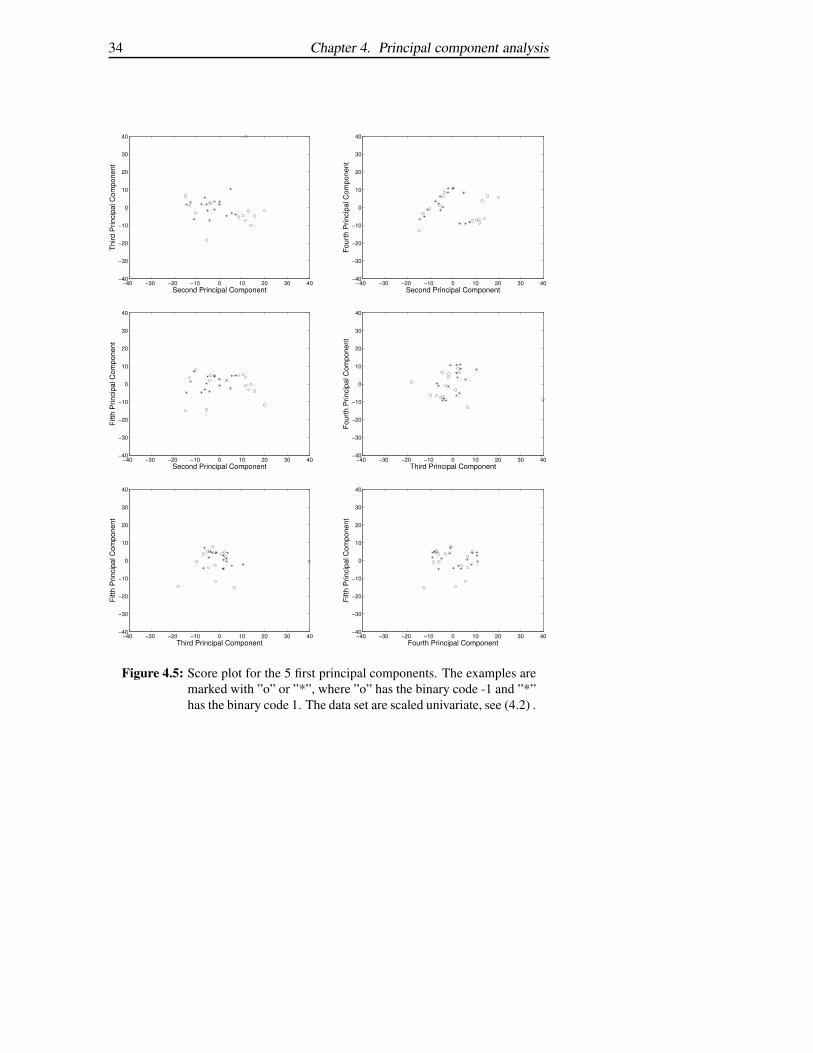
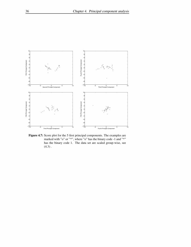
The principal components are calculated for the training set, see Section 3.6.According to Figure 4.3 (a), the number of principal components should bebetween six or seven if the ”knee” condition is used. In Figure 4.3 (b) thenumber of principal components should be 29, if Herror should be mini-mized. The purpose with principal components, to reduce the dimension,is not fulfilled according to Herror. In Figure 4.4 to 4.7 the score plots forthe five first principal components are presented. The two different scalingmethods from Section 4.3 are used. It is clearly shown in Figure 4.4 to 4.7that it is impossible to linearly separate the examples in the training set withdifferent binary code using these five principal components. Experimentshave shown that 19 principal components are needed to linearly separate theexamples.
4.5 Conclusions
In this chapter the possibility to use principal component analysis to classifythe stability of the data set presented in Chapter 3 is analyzed. Due to thecomplexity of power systems, with the large amount of variables that de-scribe the state of the system, it is not possible to use PCA to separate the

4.5. Conclusions 33
−40 −30 −20 −10 0 10 20 30 40−40
−30
−20
−10
0
10
20
30
40
First Principal Component
Sec
ond
Prin
cipa
l Com
pone
nt
−40 −30 −20 −10 0 10 20 30 40−40
−30
−20
−10
0
10
20
30
40
First Principal Component
Third
Prin
cipa
l Com
pone
nt
−40 −30 −20 −10 0 10 20 30 40−40
−30
−20
−10
0
10
20
30
40
First Principal Component
Four
th P
rinci
pal C
ompo
nent
−40 −30 −20 −10 0 10 20 30 40−40
−30
−20
−10
0
10
20
30
40
First Principal Component
Fifth
Prin
cipa
l Com
pone
nt
Figure 4.4: Score plot for the 5 first principal components. The examples aremarked with ”o” or ”*”, where ”o” has the binary code -1 and ”*”has the binary code 1. The data set are scaled univariate, see (4.2) .
examples in the training set with different binary code. A method for separa-tion in higher dimensions must be chosen to succeed with the classifications.
34 Chapter 4. Principal component analysis
−40 −30 −20 −10 0 10 20 30 40−40
−30
−20
−10
0
10
20
30
40
Second Principal Component
Third
Prin
cipa
l Com
pone
nt
−40 −30 −20 −10 0 10 20 30 40−40
−30
−20
−10
0
10
20
30
40
Second Principal Component
Four
th P
rinci
pal C
ompo
nent
−40 −30 −20 −10 0 10 20 30 40−40
−30
−20
−10
0
10
20
30
40
Second Principal Component
Fifth
Prin
cipa
l Com
pone
nt
−40 −30 −20 −10 0 10 20 30 40−40
−30
−20
−10
0
10
20
30
40
Third Principal Component
Four
th P
rinci
pal C
ompo
nent
−40 −30 −20 −10 0 10 20 30 40−40
−30
−20
−10
0
10
20
30
40
Third Principal Component
Fifth
Prin
cipa
l Com
pone
nt
−40 −30 −20 −10 0 10 20 30 40−40
−30
−20
−10
0
10
20
30
40
Fourth Principal Component
Fifth
Prin
cipa
l Com
pone
nt
Figure 4.5: Score plot for the 5 first principal components. The examples aremarked with ”o” or ”*”, where ”o” has the binary code -1 and ”*”has the binary code 1. The data set are scaled univariate, see (4.2) .

4.5. Conclusions 35
−10 −5 0 5 10−10
−8
−6
−4
−2
0
2
4
6
8
10
First Principal Component
Sec
ond
Prin
cipa
l Com
pone
nt
−10 −5 0 5 10−10
−8
−6
−4
−2
0
2
4
6
8
10
First Principal Component
Third
Prin
cipa
l Com
pone
nt
−10 −5 0 5 10−10
−8
−6
−4
−2
0
2
4
6
8
10
First Principal Component
Four
th P
rinci
pal C
ompo
nent
−10 −5 0 5 10−10
−8
−6
−4
−2
0
2
4
6
8
10
First Principal Component
Fifth
Prin
cipa
l Com
pone
nt
−10 −5 0 5 10−10
−8
−6
−4
−2
0
2
4
6
8
10
Second Principal Component
Third
Prin
cipa
l Com
pone
nt
−10 −5 0 5 10−10
−8
−6
−4
−2
0
2
4
6
8
10
Second Principal Component
Four
th P
rinci
pal C
ompo
nent
Figure 4.6: Score plot for the 5 first principal components. The examples aremarked with ”o” or ”*”, where ”o” has the binary code -1 and ”*”has the binary code 1. The data set are scaled group-wise, see(4.3) .
36 Chapter 4. Principal component analysis
−10 −5 0 5 10−10
−8
−6
−4
−2
0
2
4
6
8
10
Second Principal Component
Fifth
Prin
cipa
l Com
pone
nt
−10 −5 0 5 10−10
−8
−6
−4
−2
0
2
4
6
8
10
Third Principal Component
Four
th P
rinci
pal C
ompo
nent
−10 −5 0 5 10−10
−8
−6
−4
−2
0
2
4
6
8
10
Third Principal Component
Fifth
Prin
cipa
l Com
pone
nt
−10 −5 0 5 10−10
−8
−6
−4
−2
0
2
4
6
8
10
Fourth Principal Component
Fifth
Prin
cipa
l Com
pone
nt
Figure 4.7: Score plot for the 5 first principal components. The examples aremarked with ”o” or ”*”, where ”o” has the binary code -1 and ”*”has the binary code 1. The data set are scaled group-wise, see(4.3) .
Chapter 5
Support vector machines
This chapter is an introduction to Support Vector Machines (SVM), a newgeneration learning system based on recent advances in statistical learningtheory. Due to the large amount of variables that describe a state and thedifficulties to estimate the stability of a state SVM is used as a classifica-tion tool. The aim is to use support vectors for calculating a hyperplanein high dimensions. This hyperplane separates the data with the maximumdistance between the classes. The separation can be both linear and non-linear. The theory is applied to classification of power system stability. SVMhave been applied to real-world applications such as text categorizing, hand-written character recognition, image classification and biosequence analysis.
5.1 Linear support vector machines
SVM were introduced by Vapnik in 1992 [36] and has received considerableattention recently. The objective is to create a learning machine that respondswith a binary output to the test data. If the system sustains the dimensioncriterion it is marked by +1 otherwise it is marked -1. This designation is hereafter called the binary code. In order to train the machine, the training datamust properly describe the variations of the system. It must be consideredthat if the training data do not show enough variability, the SVM cannot besuccessfully applied.
37

38 Chapter 5. Support vector machines
5.1.1 Maximal margin optimization
Denote the training data
{xi , yi}, i = 1, . . . , l ,
where xi ∈ Rd are the input measurements and yi ∈ {−1, 1} are the corre-sponding binary responses. Suppose that there exists a hyperplane,
x ·w + b = 0 ,
with parameters (w, b), separating positive from negative examples. Let d+and d- denote the shortest distance from the hyperplane to the closest posi-tive/negative point respectively. The goal of the training is to find the hyper-plane which best separates the training data. For a linear SVM this results ina convex optimization problem, which has a global solution. The hyperplaneis therefore the plane in Rd, with the largest d+ and d-. This is a useful prop-erty that other classification methods e.g. neural networks [33] do not have.
The constraints that the hyperplane must separate the points,
xi ·w + b ≥ 0, for yi = +1
xi ·w + b ≤ 0, for yi = −1
may be combined intoyi(xi · w + b) ≥ 0 .
The points which lie on the hyperplane H1 : xi · w + b = −1 have theperpendicular distance from the origin |b − 1|/‖w‖, and the points on thehyperplane H2 : xi · w + b = 1 have the perpendicular distance from theorigin |b + 1|/‖w‖. Hence the margin is 1/||w||, see Figure 5.1.
The optimization problem{
Minimize ||w||2under the constraint di = yi(x ·w + b) ≥ 1 ,
(5.1)
can be solved, by the following transformation,
L(w, b,a) =1
2||w||2 −
l∑
i=1
aiyi(xi · w + b) +
l∑
i=1
ai , (5.2)

5.1. Linear support vector machines 39
b
wH
1
H2
d−
d+
* *
*
* *
o o
o
o
o
Figure 5.1: Linear separating hyperplane.
where a = (a1, . . . , al) are the Lagrange multipliers. The function is min-imized with respect to w and b. The constraints from the gradient of theoptimization problem with respect to w and b are
∂L(w, b,a)
∂w= w −
l∑
i=1
aiyixi = 0
∂L(w, b,a)
∂b=
l∑
i=1
aiyi = 0 .
Substituting these in (5.2) gives
L(w, b,a) =
l∑
i=1
ai −1
2
l∑
i,j=1
aiajyiyjxi · xj . (5.3)
The SVM maximizing (5.3) with respect to ai for the constraints∑
aiyi = 0and ai ≥ 0 gives the desired hyperplane. The optimization problem has aglobal solution, which gives the maximum margin between the two classes.The Karush-Kuhn-Tucker (KKT) [8] condition is used to determine b, thedistance from the origin to the hyperplane, see Figure 5.1.

40 Chapter 5. Support vector machines
According to the KKT condition
ai(yi(xi · w + b) − 1) = 0 .
This can be used to determine b for any i for which ai > 0. Every trainingpoint xi has a corresponding ai. The points which correspond to ai > 0 arecalled support vectors. These points lie on the hyperplanes, H1 and H2
and affect the decision of the machine.The classification data can be classified with the hyperplane using the sign
of the function
f(x) = x ·w + b =
l∑
i=1
aiyixi · x + b . (5.4)
5.1.2 Soft margin optimization
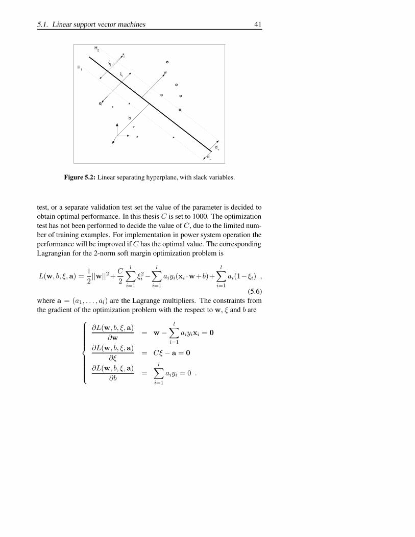
The maximal margin optimization calculates a hyperplane with a consistenthypothesis. The resulting distance between the two classes is always thelargest possible distance. In some classification problems it is not desirableto use the maximal margin optimization. If an example in the training setconsists of misleading data the hyperplane will be affected by this. There-fore soft margin optimization can be used to calculate a hyperplane, whichpermit some degree of incorrect separation. This hyperplane represents asimpler model than the possibly over-fitted hyperplane of the maximal mar-gin classifier. The so called slack variables ξ are used to represent the in-correct separation, see Figure 5.2. The hyperplane is calculated from thefollowing optimization problem, for details see [8].
2-Norm Soft Margin
Using the 2-norm for the slack variable, the optimization problem is
Minimize ||w||2 + C
l∑
i=1
ξ2i
under the constraint di = yi(x · w + b) ≥ 1 − ξi ,
(5.5)
where ξ = (ξ1, . . . , ξl) are the slack variables. The variable C must be cho-sen from a wide range of values. By using cross validation, leave-one-out
5.1. Linear support vector machines 41
b
wH
1
H2
d−
d+
* *
*
* *
o o
o
o
o
*j
ξj
o
ξi
i
Figure 5.2: Linear separating hyperplane, with slack variables.
test, or a separate validation test set the value of the parameter is decided toobtain optimal performance. In this thesis C is set to 1000. The optimizationtest has not been performed to decide the value of C , due to the limited num-ber of training examples. For implementation in power system operation theperformance will be improved if C has the optimal value. The correspondingLagrangian for the 2-norm soft margin optimization problem is
L(w, b, ξ,a) =1
2||w||2 +
C
2
l∑
i=1
ξ2i −
l∑
i=1
aiyi(xi ·w+b)+l∑
i=1
ai(1−ξi) ,
(5.6)where a = (a1, . . . , al) are the Lagrange multipliers. The constraints fromthe gradient of the optimization problem with the respect to w, ξ and b are
∂L(w, b, ξ,a)
∂w= w −
l∑
i=1
aiyixi = 0
∂L(w, b, ξ,a)
∂ξ= Cξ − a = 0
∂L(w, b, ξ,a)
∂b=
l∑
i=1
aiyi = 0 .

42 Chapter 5. Support vector machines
Substituting these in (5.6) gives
L(w, b,a) =
l∑
i=1
ai −1
2
l∑
i,j=1
aiajyiyjxi · xj −1
2C
l∑
i=1
a2i . (5.7)
The SVM maximizing (5.7) with respect to ai, for the constraints∑aiyi = 0 and ai ≥ 0, gives the desired hyperplane.According to the KKT condition b is determined with
ai(yi(x ·w + b) − 1 + ξi) = 0 ,
for any ai > 0.
1-Norm Soft Margin
Using the 1-norm for the slack variable, the optimization problem is
Minimize ||w||2 + C
l∑
i=1
ξi
under the constraint di = yi(x ·w + b) ≥ 1 − ξi
ξi ≥ 0 .
(5.8)
The 1-norm soft margin is refered to as ”the Box Constraint”, where ξi < C .The difference between 1-norm and 2-norm is that ξi is limited by C for 1-norm, and not by 2-norm. The corresponding Lagrangian for the 1-norm softmargin optimization problem is
L(w, b, ξ,a, r) =1
2||w||2+C
l∑
i=1
ξi−l∑
i=1
aiyi(xi·w+b−1+ξi)+l∑
i=1
riξi ,
(5.9)where a and r are the Lagrange multipliers. The function is minimized withrespect to w, ξ. The constrains from the gradient of the optimization problemwith the respect to w, ξ and b are
∂L(w, b, ξ,a, r)
∂w= w −
l∑
i=1
aiyixi = 0
∂L(w, b, ξ,a, r)
∂ξi
= C − ai − ri = 0
∂L(w, b, ξ,a, r)
∂b=
l∑
i=1
aiyi = 0 .

5.2. Scaling 43
Substituting these in (5.9) gives
L(w, b,a) =
l∑
i=1
ai −1
2
l∑
i,j=1
aiajyiyjxi · xj , (5.10)
which is identical with the maximal margin. The only difference is the de-termination if b with the KKT condition
{ai(yi(x · w + b) − 1 + ξi) = 0ξi(ai − C) = 0 ,
for any ai > 0.
5.2 Scaling
As in Chapter 4 the data set is preprocessed before calculation of the hyper-plane. In practice, the examples in the data set xi are stored as rows in amatrix. The columns z = (z1, . . . , zl) of this matrix are scaled to a prede-fined interval with a linear scaling [17],
zlinear =2(z − Min)
Max − Min− 1 (5.11)
Min = The smallest value in every column
Max = The largest value in every column.
5.2.1 Scaling to keep the physical properties
The scaling method that keeps the physical properties of the variables, whichwas introduced in Chapter 4, is also used to classify with SVM. It is hereapplied to the linear scaling. First, the voltage V and I are calculated in p.u.[13] as
Vp.u. =V
Vbase
and Ip.u. =I
Ibase
,
with a common system base Sbase. Which results in,
Ibase =Sbase√3Vbase
.

44 Chapter 5. Support vector machines
Then the variables are divided into groups e.g. busbar V, load P, line I andangle differences. The groups are scaled with the linear function (5.11).Instead of finding Min and Max in every column, the Min and Max valuesare found in groups of variables which are then scaled group-wise.
5.2.2 Scaling of unit stator current after capacity
The capacity of the power system to fulfil the (n − 1) criterion depends onthe spinning reserve. Therefore this is used to improve the classification.Instead of using the unit stator currents in the data set the stator current isused to calculate the unit capacity to increase the production. When thestator current is used in the data set no consideration of the unit capacity istaken. If a unit is idle, the stator current is almost 0. The unit has a largecapacity to prevent a stressed situation. When a unit is not connected to thepower system the stator current is 0, but the unit has no capacity to preventa stressed situation. Both units have almost the same stator current, but thecapacity to prevent a stressed situation is totaly different. Instead of usingIp.u., I∗ is calculated as
I∗ =Irated − I
Ibase
,
were Irated is on machine base. Using I∗ the influence of the hyperplanefrom a unit in nominal production and a disconnected unit are the same.
5.2.3 Variables
In total 653 variables are used in an example to describe the operating pointof the power system, post-fault. The variables are
• P, Q and I for lines, (156)
• V, f for busbars, (64)
• P, Q and I for loads, (180)
• P, Q and I for transformers, (24)
• P, Q and I for units, (108)
• Q and I for shunts, (84)
5.3. SVM training 45
• Angle differences, (37),
where the number of variables in each group are shown in parenthesis.
5.3 SVM training
Using the OSU SVM matlab toolbox [27] the support vectors are calculated.The number of support vectors is 20. The support vectors are used with (5.9)to calculate the hyperplane. The hyperplane is the optimal linear separationbetween the two classes. Using (5.4), the function value for each of theexamples in the training set is decided.
In Figure 5.3 (a)-(c) the function value for the 30 examples in the trainingset are marked by a ”o” or ”*” (”o” has the binary code -1 and ”*” +1). Theexamples which are used as support vectors have the function value ±1, asin Figure 5.3 (a)-(c). It is possible to find a hyperplane which separates thetwo classes in the training set, scaled by 3 different methods, with SVM.
In Section 3.3 one of the traditional methods to indicate if the (n − 1) isfulfilled in the Swedish part of the Nordel system, the cut-sets methodologywas introduced. Figure 5.4 shows that it is difficult to use the cut-sets toclassify the stability of the examples in the training set. The examples withdifferent binary code can not be separated with a certain threshold.
As the number of available examples is small, the performance of thetraining set is validated by leave-one-out cross validation, see [38]. Eachtime 29 of the 30 examples in the training set are used to train the SVM.The remaining example is then used for classification. This is done for all 30examples, see Figure 5.3 (d). With the leave-one-out test 28 of 30 examplesin the training set are correctly classified. The robustness in the training setis pretty good with a fault classification of 28/30.

46 Chapter 5. Support vector machines
0 5 10 15 20 25 30−3
−2
−1
0
1
2
3
Example
Func
tion
valu
e
0 5 10 15 20 25 30−3
−2
−1
0
1
2
3
Example
Func
tion
valu
e
(a) (b)
0 5 10 15 20 25 30−3
−2
−1
0
1
2
3
Example
Func
tion
valu
e
0 5 10 15 20 25 30−3
−2
−1
0
1
2
3
Example
Func
tion
valu
e
(c) (d)
Figure 5.3: Linear SVM with soft-margin optimization, where C = 1000. Ex-amples marked with ”o” has the binary code -1 and ”*” has thebinary code +1. The function value, see (5.4), for the training set.All 633 feature variables are used, 20 variables are excluded dueto variance equal to 0. (a) The variables are scaled linear group-wise, the unit stator current are also scaled after capacity. (b) Thevariables scaled linear group-wise. (c) The variables scaled lin-ear separately. (d) Leave-one-out test. The function value, for thetraining set, 28 of 30 examples are correctly classified. The vari-ables are scaled as in (b).

5.4. Classifying with a hyperplane 47
0 5 10 15 20 25 300
500
1000
1500
2000
2500
3000
3500
Example
Cut
−set
val
ue
0 5 10 15 20 25 300
200
400
600
800
1000
1200
1400
1600
1800
2000
Example
Cut
−set
val
ue
(a) (b)
Figure 5.4: (a) The sum of transferred active power through Snitt2, for theexamples in the training set. (b) Snitt4, for the examples in thetraining set.
5.4 Classifying with a hyperplane
The hyperplane described in Section 5.3 is used to classify the examples inthe classification set. With Equation (5.4) the function value is decided. Theclassification set is scaled with the three methods, which corresponds to theexamples in the training set. In Figure 5.5 (a)-(c) the function value, for theexamples in the classification set are marked as in Figure 5.3.
The four examples that are misclassified are classified to fulfill the (n−1)criterion, but they do not. The examples are originally represented in thetraining set and there they fulfill (n − 1), but in the classification set theactive power load is increased on a common system base so they do not. Thefaults which make the examples to not fulfill the (n − 1) are short circuit ofbusbar CT11_ B400, CT21_ A400 and FT50_ A400, see Figure 3.2. Thesefaults also cause blackouts for the examples in the training set so the faultsare represented both in the training and classification set.
The misclassification depends on that the training set has too few ex-amples, or that the variability of the examples in the training set does notdescribe the examples in the classification set. If the training set does notdescribe the examples in the classification set it is impossible to make acorrect classification. The number of variables used to describe the clas-

48 Chapter 5. Support vector machines
sification problem can also be too large, thus the hyperplane is over-fitted,see Figure 5.6. The hyperplane is over-fitted if the hyperplane is adjusted tothe training set instead of the classification problem, which hopefully is de-scribed by the training set. The linear SVM decreases the risk for overfitting,compared to using a nonlinear function. There is a need to investigate if theclassification can be improved with fewer variables.
As with the examples in the training set the cut-set methodology is notsuccessful to use to classify the examples in the classification set, see Fig-ure 5.7. The examples with different binary code can not be separated witha threshold.

5.4. Classifying with a hyperplane 49
0 2 4 6 8 10 12 14 16−3
−2
−1
0
1
2
3
Example
Func
tion
valu
e
0 2 4 6 8 10 12 14 16−3
−2
−1
0
1
2
3
ExampleFu
nctio
n va
lue
(a) (b)
0 2 4 6 8 10 12 14 16−20
−15
−10
−5
0
5
10
15
20
Example
Func
tion
valu
e
(c)
Figure 5.5: Linear SVM classification with soft-margin optimization, whereC = 1000. Examples marked with ”o” has the binary code -1 and”*” has the binary code +1. (a) The function value, for the clas-sification set. All 633 feature variables are used and scaled lineargroup-wise, the unit stator current are also scaled after capacity .(b) The function value, for the classification set. All 633 featurevariables, scaled linear group-wise. (c) The function value, for thetraining set. All 633 features variables scaled linear separately.

50 Chapter 5. Support vector machines
Figure 5.6: Illustration of overfitting classification.
0 2 4 6 8 10 12 14 160
500
1000
1500
2000
2500
3000
3500
Example
Cut
−set
val
ue
0 2 4 6 8 10 12 14 160
200
400
600
800
1000
1200
1400
1600
1800
2000
Example
Cut
−set
val
ue
(a) (b)
Figure 5.7: (a) Snitt2, for the classification set. (b) Snitt4, for the classificationset.

5.5. Reducing variable sets 51
5.5 Reducing variable sets
There is a need to analyze if the original data set consists of variables whichcause over-fitting problems. The problem is, given the original data set inRd, what is the best subset of feature variables in Rc, where c<d? It is notpossible to find an optimal solution for this problem. First of all, we do notknow the dimension of Rc and if we knew it, the number of possible subsetsis
nc =d!
(d − c)!c!
which is very large when d is 650.Therefore, a new method to reduce the dimension of the data set is intro-
duced, thus reducing the dimension of the data set without removing vari-ables which are important for the separation. First, all variables in the train-ing data with zero variance are removed. Then a method for further reductionis introduced. To reduce the variables the whole training data is scaled ac-cording to (5.11), and a hyperplane is calculated with SVM. By guidancefrom the normal w of the hyperplane, the dimension of the training set isreduced.
The unit normal of the hyperplane wn is calculated, as
wn =w
||w|| . (5.12)
The absolute value of the j’th component in wn indicates the contributionof the j’th variable to the hyperplane, see Figure 5.8. All components lowerthan a certain threshold, heuristically found, are removed. This procedure isimportant to analyze, so that over-fitting problems can be avoided.
The reduction method is applied on the data set, where the variables arereduced by guidance from the normal to the hyperplane. After the reduction anew hyperplane is calculated with the new variable setup. Then the functionvalue for the examples in the classification set is calculated.
Only 2 of 16 are misclassified, both with the original variable setup andwhen the number of variables is reduced from 633 to 70, see Figure 5.9. Thevariables that are used to describe the classification problem after reductionare,

52 Chapter 5. Support vector machines
ej
w
Figure 5.8: Reducing variables by guidance form the normal of the hyper-plane.
• P, Q and I for lines, (0, 9, 16 of 156)
• V, f for busbars, (5, 0 of 64)
• P, Q and I for loads, (0, 0, 0 of 180)
• P, Q and I for transformers, (0, 0, 0 of 24)
• P, Q and I for units, (3, 6, 1 of 108)
• Q and I for shunts, (11, 16 of 84)
• Angle differences, (2 of 37),
where the numbers of variables in each group is shown, ordered from left toright, in parenthesis.
5.5.1 Different variable setup
In [11], [14] and [28] it is indicated that variable have different variations pat-terns. Consideration must be taken about the difference between variables.

5.5. Reducing variable sets 53
0 2 4 6 8 10 12 14 16−3
−2
−1
0
1
2
3
Example
Func
tion
valu
e
0 2 4 6 8 10 12 14 16−3
−2
−1
0
1
2
3
Example
Func
tion
valu
e
(a) (b)
Figure 5.9: Linear SVM classification with soft-margin optimization, whereC = 1000. Examples marked with ”o” has the binary code -1 and”*” has the binary code +1. The variables are scaled linear group-wise, the unit stator current are also scaled after capacity. (a) All633 feature variables. (b) The 70 variables which have the largestinfluence on the hyperplane.
The variables can be divided into two groups:
• Qualitative
• Quantitative
Qualitative variables are normally represented numerically by codes. Theeasiest representation is a single binary code as 0 or 1, e.g. circuit breakersstatus. In this study circuit breakers/disconectors are not used in the data set,but shunt capacitors and reactors are included in the data set and they areapproximately qualitative.
Quantitative variables may assume any numerical value along a continu-ous scale. All variables in the data set are of this type except shunts. It isimportant to be aware of the difference between the two variable types.
There is a need to investigate if the number of variables that are used forclassification can be reduced. Large data sets can cause over-fitting prob-lems, it is also interesting to minimize the cost to measure and collect thedata set. Therefore the different variable groups are used, one-at-a-time, tocalculate the hyperplane with soft margin optimization. The variables are

54 Chapter 5. Support vector machines
scaled group-wise, unit stator current is also scaled after capacity. In Figures5.10-5.12 the results with the different variables are shown, some variablesgive a better hyperplane for separation than others. The load and frequencygives an unsatisfactory separation while line and voltage gives successfulseparation.

5.5. Reducing variable sets 55
0 5 10 15 20 25 30−30
−20
−10
0
10
20
30Bus voltage
Example
Func
tion
valu
e
0 5 10 15 20 25 30−30
−20
−10
0
10
20
30
Example
Func
tion
valu
e
P load
0 5 10 15 20 25 30−30
−20
−10
0
10
20
30
Example
Func
tion
valu
e
Q load
0 5 10 15 20 25 30−30
−20
−10
0
10
20
30
Example
Func
tion
valu
e
I load
0 5 10 15 20 25 30−30
−20
−10
0
10
20
30
Example
Func
tion
valu
e
Q shunt
0 5 10 15 20 25 30−30
−20
−10
0
10
20
30
Example
Func
tion
valu
e
I shunt
Figure 5.10: The function value for the SVM training based on the differentvariable groups in the training set. The soft-margin optimizationis used to calculate a hyperplane with slack variables, where C =1000, for further information see Section 5.1.2. The variables arescaled group-wise, where the unit stator current also are scaledafter capacity.
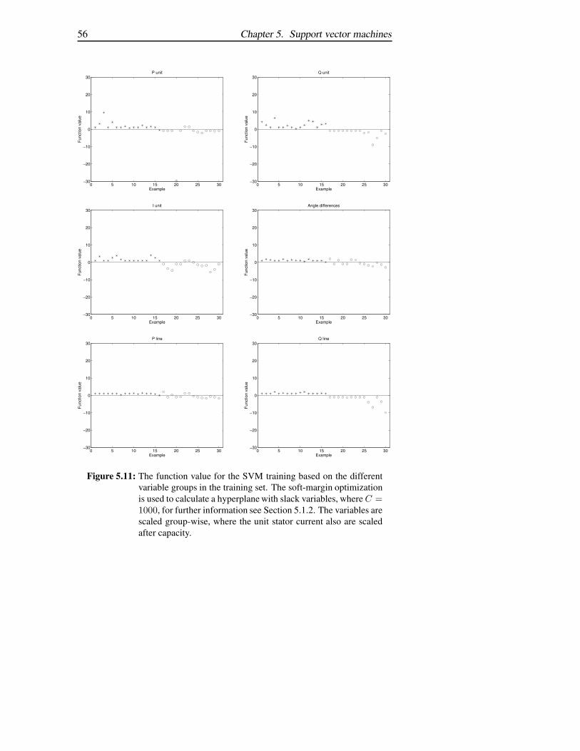
56 Chapter 5. Support vector machines
0 5 10 15 20 25 30−30
−20
−10
0
10
20
30
Example
Func
tion
valu
e
P unit
0 5 10 15 20 25 30−30
−20
−10
0
10
20
30
Example
Func
tion
valu
e
Q unit
0 5 10 15 20 25 30−30
−20
−10
0
10
20
30
Example
Func
tion
valu
e
I unit
0 5 10 15 20 25 30−30
−20
−10
0
10
20
30
Example
Func
tion
valu
e
Angle differences
0 5 10 15 20 25 30−30
−20
−10
0
10
20
30
Example
Func
tion
valu
e
P line
0 5 10 15 20 25 30−30
−20
−10
0
10
20
30
Example
Func
tion
valu
e
Q line
Figure 5.11: The function value for the SVM training based on the differentvariable groups in the training set. The soft-margin optimizationis used to calculate a hyperplane with slack variables, where C =1000, for further information see Section 5.1.2. The variables arescaled group-wise, where the unit stator current also are scaledafter capacity.

5.5. Reducing variable sets 57
0 5 10 15 20 25 30−30
−20
−10
0
10
20
30
Example
Func
tion
valu
e
I line
0 5 10 15 20 25 30−30
−20
−10
0
10
20
30
Example
Func
tion
valu
e
P transformer
0 5 10 15 20 25 30−30
−20
−10
0
10
20
30
Example
Func
tion
valu
e
Q transformer
0 5 10 15 20 25 30−30
−20
−10
0
10
20
30
Example
Func
tion
valu
e
I transformer
0 5 10 15 20 25 30−30
−20
−10
0
10
20
30
Example
Func
tion
valu
e
Frequency
Figure 5.12: The function value for the SVM training based on the differentvariable groups in the training set. The soft-margin optimizationis used to calculate a hyperplane with slack variables, where C =1000, for further information see Section 5.1.2. The variables arescaled group-wise, where the unit stator current also are scaledafter capacity.

58 Chapter 5. Support vector machines
0 5 10 15 20 25 30−2
−1.5
−1
−0.5
0
0.5
1
1.5
2
Example
Sca
led
varia
ble
valu
e
Figure 5.13: Two of the variables in the training set, scaled linear group-wise,CT22 X1 CurrentValue, qualitative, marked with ”�” and CT22A400 VoltageValue, quantitative, marked with ”+”.
It is possible to calculate a hyperplane that separates the examples in thetraining set with both P shunt and I shunt. Therefore, it should be naturalto use the two variable classes for the classification problem. But P shuntand I shunt are qualitative and therefore they have too large impact on thehyperplane. The hyperplane will then be trained to classify between twodifferent shunt patterns that can be identified in the training set. In Table 5.1the 30 variables which have the largest impact on the hyperplane are listed,19 of these are shunts. The difference between qualitative and quantitativevariables are shown in Figure 5.13. It is well known that mixing qualitativeand quantitative variables can give problems when building classifiers. Thereare methods for dealing with this, e.g. [21] and [38]. Usually these methodsrequire large training sets.

5.5. Reducing variable sets 59
Table 5.1: The 30 variables which have the largest influence on the hyperplane.The soft-margin optimization is used to calculate a hyperplane withslack variables, where C = 1000, for further information see Sec-tion 5.1.2. The variables are scaled group-wise, where the unit sta-tor current also are scaled after capacity.
Object w
||w||
CT22 X1 Shunt reactor (I) 0.4675CT32 X3 Shunt reactor (I) 0.3942CT22 X1 Shunt reactor (Q) 0.2635FT41 EK1 Shunt capacitor (I) 0.2276CT32 X3 Shunt reactor (Q) 0.2243CT31 X3 Shunt reactor (I) 0.2124FT42 X1 Shunt reactor (I) 0.1483FT44 X1 Shunt reactor (I) 0.1419FT50 X1 Shunt reactor (I) 0.1410CT11 T2 Unit (Q) 0.1364FT41 EK1 Shunt capacitor (Q) 0.1309CT21 X1 Shunt reactor (I) 0.1225CT31 X3 Shunt reactor (Q) 0.1207CT11 X1 Shunt reactor (I) 0.1100CT32 X1 Shunt reactor (I) 0.1075CT22 A400 Busbar (V) 0.0871CL1 Line (I) CT11 0.0867FT42 X1 Shunt reactor (Q) 0.0837FT44 X1 Shunt reactor (Q) 0.0810FT44 T11 Unit (Q) 0.0799FT50 X1 Shunt reactor (Q) 0.0773FT51 G2 Unit (Q) 0.0752FT50 X2 Shunt reactor (I) 0.0743CT72 G2 Unit (P) 0.0733CL8 Line (Q) CT22 0.0727CT122 A130 Busbar (V) 0.0718CT21 X1 Shunt reactor (Q) 0.0695FL14 Line (I) FT51 0.0690FL15 Line (I) FT51 0.0690CL3 Line (Q) CT22 0.0671

60 Chapter 5. Support vector machines
Due to the different variable types, different variable setups are applied toclassification with SVM. In Section 5.4 the data set was scaled with threedifferent methods. All three are also used here because no method could beexcluded from the results in Section 3. Five variable setups are compared,
1. Original variable setup, 653
2. Shunts removed, 569
3. All P and Q removed, 289
4. All P and Q, transformer and shunts removed, 257
5. All P and Q, frequency and shunts removed, 225
and the data set is scaled by three different methods,
1. Group-wise
2. Group-wise, unit stator current is also scaled by capacity
3. Separately.
The variable setup which gives the best separation are 2, 4 and 5.

5.5. Reducing variable sets 61
0 2 4 6 8 10 12 14 16−20
−15
−10
−5
0
5
10
15
20
Example
Func
tion
valu
e
Variable setup 1, scaling method 1
0 2 4 6 8 10 12 14 16−20
−15
−10
−5
0
5
10
15
20
Example
Func
tion
valu
e
Variable setup 1, scaling method 2
0 2 4 6 8 10 12 14 16−20
−15
−10
−5
0
5
10
15
20
Example
Func
tion
valu
e
Variable setup 1, scaling method 3
0 2 4 6 8 10 12 14 16−20
−15
−10
−5
0
5
10
15
20
Example
Func
tion
valu
eVariable setup 2, scaling method 1
0 2 4 6 8 10 12 14 16−20
−15
−10
−5
0
5
10
15
20
Example
Func
tion
valu
e
Variable setup 2, scaling method 2
0 2 4 6 8 10 12 14 16−20
−15
−10
−5
0
5
10
15
20
Example
Func
tion
valu
e
Variable setup 2, scaling method 3
Figure 5.14: The function value for the SVM classification based on the dif-ferent variable setups and different scaling methods. The soft-margin optimization is used to calculate a hyperplane with slackvariables, where C = 1000.

62 Chapter 5. Support vector machines
0 2 4 6 8 10 12 14 16−20
−15
−10
−5
0
5
10
15
20
Example
Func
tion
valu
eVariable setup 3, scaling method 1
0 2 4 6 8 10 12 14 16−20
−15
−10
−5
0
5
10
15
20
Example
Func
tion
valu
e
Variable setup 3, scaling method 2
0 2 4 6 8 10 12 14 16−20
−15
−10
−5
0
5
10
15
20
Example
Func
tion
valu
e
Variable setup 3, scaling method 3
0 2 4 6 8 10 12 14 16−20
−15
−10
−5
0
5
10
15
20
Example
Func
tion
valu
e
Variable setup 4, scaling method 1
0 2 4 6 8 10 12 14 16−20
−15
−10
−5
0
5
10
15
20
Example
Func
tion
valu
e
Variable setup 4, scaling method 2
0 2 4 6 8 10 12 14 16−20
−15
−10
−5
0
5
10
15
20
Example
Func
tion
valu
e
Variable setup 4, scaling method 3
Figure 5.15: The function value for the SVM classification based on the dif-ferent variable setups and different scaling methods. The soft-margin optimization is used to calculate a hyperplane with slackvariables, where C = 1000.

5.5. Reducing variable sets 63
0 2 4 6 8 10 12 14 16−20
−15
−10
−5
0
5
10
15
20
Example
Func
tion
valu
e
Variable setup 5, scaling method 1
0 2 4 6 8 10 12 14 16−20
−15
−10
−5
0
5
10
15
20
Example
Func
tion
valu
e
Variable setup 5, scaling method 2
0 2 4 6 8 10 12 14 16−20
−15
−10
−5
0
5
10
15
20
Example
Func
tion
valu
e
Variable setup 5, scaling method 3
Figure 5.16: The function value for the SVM classification based on the dif-ferent variable setups and different scaling methods. The soft-margin optimization is used to calculate a hyperplane with slackvariables, where C = 1000.

64 Chapter 5. Support vector machines
The method to reduce variables by guidance from the normal to the hy-perplane is applied to the data sets with the variable setups which give thebest classification, according to Figure 5.14-5.16. The variable setups withshunts are excluded. The linear scaling method is not used. The reductionis illustrated with a new plot, reduction plot, which shows the number ofcorrect classified examples in the classification set. The number of variablesin the data set is reduced by two different reduction methods:
1. The first one by increasing the threshold so one variable is excluded ata time, see Figure 5.17-5.18.
2. The other is by excluding the variable which has the least influenceon the hyperplane, the new data set is used to calculate the differencebetween the variables. Thereafter a new hyperplane is calculated andthe process is repeated, see Figure 5.19-5.20.
The variable groups that are dominating in the reduction process are pre-sented in Table 5.2. The variable setups that have varying classification resultare divided into subsets, see Figure 5.17-5.20. In these subsets the dominat-ing variable groups are presented in Table 5.2. This is only a guideline ofwhich variable groups that are excluded, there are other variable groups rep-resented in the subsets. In Table 5.3 the 30 variables which have the largestimpact on the hyperplane are listed. The variable setup where P, Q, trans-former and shunt are reduced is used. These 30 variables are also pointedout in Figure 5.21.

5.5. Reducing variable sets 65
0 100 200 300 400 5000
2
4
6
8
10
12
14
16
Variable setup 2, scaling method 1, reduction method 1
Number of variables
Cor
rect
cla
ssifi
catio
ns
4
123
0 100 200 300 400 5000
2
4
6
8
10
12
14
16
Variable setup 2, scaling method 2, reduction method 1
Number of variables
Cor
rect
cla
ssifi
catio
ns
4
3 2 1
(a) (b)
0 50 100 150 200 2500
2
4
6
8
10
12
14
16
Variable setup 4, scaling method 1, reduction method 1
Number of variables
Cor
rect
cla
ssifi
catio
ns
4
3 2 1
0 50 100 150 200 2500
2
4
6
8
10
12
14
16
Variable setup 4, scaling method 2, reduction method 1
Number of variables
Cor
rect
cla
ssifi
catio
ns
12
3
(c) (d)
Figure 5.17: The reduction plot based on the different variable setups and dif-ferent scaling methods. The x-axis show the numbers of variablesthat are used in the classification. The y-axis show the numberof correct classified examples in the classification set. The soft-margin optimization is used to calculate a hyperplane with slackvariables, where C = 1000.

66 Chapter 5. Support vector machines
0 50 100 150 2000
2
4
6
8
10
12
14
16
Variable setup 5, scaling method 1, reduction method 1
Number of variables
Cor
rect
cla
ssifi
catio
ns
123
4
0 50 100 150 2000
2
4
6
8
10
12
14
16
Variable setup 5, scaling method 2, reduction method 1
Number of variables
Cor
rect
cla
ssifi
catio
ns
12
3
(a) (b)
Figure 5.18: The reduction plot based on the different variable setups and dif-ferent scaling methods. The x-axis show the numbers of variablesthat are used in the classification. The y-axis show the numberof correct classified examples in the classification set. The soft-margin optimization is used to calculate a hyperplane with slackvariables, where C = 1000.

5.5. Reducing variable sets 67
0 100 200 300 400 5000
2
4
6
8
10
12
14
16
Number of variables
Cor
rect
cla
ssifi
catio
ns
Variable setup 2, scaling method 1, reduction method 2
0 100 200 300 400 5000
2
4
6
8
10
12
14
16
Number of variables
Cor
rect
cla
ssifi
catio
ns
Variable setup 2, scaling method 2, reduction method 2
(a) (b)
0 50 100 150 200 2500
2
4
6
8
10
12
14
16
Number of variables
Cor
rect
cla
ssifi
catio
ns
Variable setup 4, scaling method 1, reduction method 2
0 50 100 150 200 2500
2
4
6
8
10
12
14
16
Number of variables
Cor
rect
cla
ssifi
catio
ns
Variable setup 4, scaling method 2, reduction method 2
(c) (d)
Figure 5.19: The reduction plot based on the different variable setups and dif-ferent scaling methods. The x-axis show the numbers of variablesthat are used in the classification. The y-axis show the numberof correct classified examples in the classification set. The soft-margin optimization is used to calculate a hyperplane with slackvariables, where C = 1000.

68 Chapter 5. Support vector machines
0 50 100 150 2000
2
4
6
8
10
12
14
16
Number of variables
Cor
rect
cla
ssifi
catio
ns
Variable setup 5, scaling method 1, reduction method 2
1234
0 50 100 150 2000
2
4
6
8
10
12
14
16
Number of variables
Cor
rect
cla
ssifi
catio
ns
Variable setup 5, scaling method 2, reduction method 2
123
(a) (b)
Figure 5.20: The reduction plot based on the different variable setups and dif-ferent scaling methods. The x-axis show the numbers of variablesthat are used in the classification. The y-axis show the numberof correct classified examples in the classification set. The soft-margin optimization is used to calculate a hyperplane with slackvariables, where C = 1000.

5.5. Reducing variable sets 69
Table 5.2: The dominating variable groups that are excluded in the reductionin Figure 5.17-5.201 2 3 4
5.17 (a) Load (P, Q) Load (I)Angle differ-ence
Mixture ofall variables
Line (P, Q, I)Unit (P, Q I)Busbar (V)
5.17 (b) Load (P, Q) Load (I)Line (P)
Mixture ofall variables
Line (P, Q, I)Unit (P, Q I)Busbar (V)
5.17 (c) Load (I)Busbar (f)
Load (I)Unit (I)
Line (I)Angle differ-ence
Line (I)Busbar (V)Angle differ-ence
5.17 (d) Load (I)Busbar (f)
Line (I)Unit (I)Angle differ-ence
Busbar (V)Line (I)
5.18 (a) Load (I) Line (I)Load (I)Angle differ-ence
Line (I)Angle differ-enceBusbar (V)
Line (I)Busbar (V)Unit (I)
5.18 (b) Angle differ-enceLine (I)Load (I)
Line (I)Busbar (V)Unit (I)
Line (I)Busbar (V)
5.20 (a) Load (I) Load (I) Angle differ-enceLine (I)Unit (I)
Line (I)Busbar (V)
5.20 (b) Mixture ofall variables
Mixture ofall variables
Busbar (V)

70 Chapter 5. Support vector machines
Table 5.3: The 30 variables which have the largest influence on the hyperplanein Figure 5.17, variable setup 4, scaling method 2 and reductionmethod 1.
Object w
||w||
CT11 A400 Busbar (V) 0.3245FT44 A400 Busbar (V) 0.3212CT22 A400 Busbar (V) 0.3100CT111 A130 Busbar (V) 0.2843CT122 A130 Busbar (V) 0.2272FL2 Line (I) FT42 0.2249FL6 Line (I) FT61 0.1983FT41 A400 Busbar (V) 0.1708CT21 A400 Busbar (V) 0.1678CL1 Line (I) CT11 0.1656CL5 Line (I) CT12 0.1560CT12 A400 Busbar (V) 0.1474CT72 G2 Unit (I) 0.1423FT41 G1 Unit (I) 0.1260CT72 G3 Unit (I) 0.1201AT111 A130 Busbar (V) 0.1189CL4 Line (I) CT12 0.1121CT112 A130 Busbar (V) 0.1071CL7 Line (I) CT71 0.1065CL6 Line (I) CT71 0.1065FL3 Line (I) FT43 0.1047FT42 A400 Busbar (V) 0.0956FT142 A130 Busbar (V) 0.0937CT11 T1 Unit (I) 0.0913FL10 Line (I) FT62 0.0889CL17 Line (I) FT44 0.0878FL15 Line (I) FT51 0.0855FL14 Line (I) FT51 0.0855FT50 A400 Angle FT62 A400 0.0852RT132 G1 Unit (I) 0.0851

5.5. Reducing variable sets 71
Figure 5.21: The NORDIC32 system with the variables from Table 5.3marked. Bus voltage are marked with ”V”, unit stator currentwith ”U” and line current with ”—”.

72 Chapter 5. Support vector machines
5.6 Implementation
It is not a problem to calculate a hyperplane which can be used to classify thestability of the NORDEL power system. The calculation time for a trainingset which consists of 12000 examples and 1200 variables takes 3,3 s1 and todecide the function value for an example with Equation 5.4 takes 0,04 s. Theproblem is to obtain a training set which is representative for the NORDELsystem. The SCADA system gives the possibility to measure and collect thedata. But for each of the examples, which can be measured and collected,it is impossible to decide the binary code. An example can obviously bemodelled in a simulator, for example ARISTO, and the binary code can bedecided for the model. But it is important to be aware of the differencebetween model and reality. The questions that have to be investigated beforeimplementing this technique are:
• Is it possible to produce a training set with a model of the power sys-tem and use the training set to classify the stability of the real powersystem?
• Is it possible to classify an example, without having verified that thetraining set is representative for the classification example?
• What happens when a part of the data is misleading and contains mea-surement errors?
The author considers that it is possible to produce a training set in a sim-ulator, it is mainly based on the methods which are used today in the stateestimators. But the training set must be representative for the power systemand the amount of time to produce such a training set will be very large. In[39] the system that have been used consists of 561 buses, 1000 lines and 61generators. The number of examples in the data base are 11 000. The sec-ond question inspires for further research in this area, especially in findingmethods to verify if it is possible to classify an example with the existingtraining set. The last question is not a large problem if the misleading datais identified. Robustness studies must be made of which variables that canbe excluded. If the misleading data can be excluded the calculation time toremove these variables and calculate a new hyperplane is not a problem.
1On a 1,6 GHz Intel centrino PC with 512 MB RAM-memory and Windows XP usingMatlab 6.5.

5.7. Results 73
5.7 Results
Classification of the stability of the NORDIC32 system with a linear SVMshows that it is not enough to use the cut-sets methodology as indicationof instability, which is mainly used in the Nordic power system today, seeFigure 5.4 and 5.7. The examples with different binary code can not beseparated using the power flow through the cut-sets.
In Section 5.3 it is shown that a hyperplane can be calculated that separatesthe examples with different binary code. But due to the misclassifications inthe classification set, see Figure 5.5, different variable setups, scaling meth-ods and a reduction method to improve the classification are used. In Figure5.12 the different groups of variables are used one-at-a-time to calculate ahyperplane with soft-margin SVM. Some variable groups are more suitableto use for the classification than others. The difference between qualitativeand quantitative variables must be noticed. In Table 5.1 it can be seen that18 of the 30 variables that have the largest influence on the hyperplane arequalitative. It is reasonable to assume that the qualitative variables contributeto an over-fitted hyperplane which classifies the disconnection of shunt re-actors and capacitors instead of the stability of the power system, see Figure5.13. When the qualitative variables are excluded from the data set the clas-sification is improved. The number of correct classification and the distancebetween the two classes is increased.
In this chapter a new method to scale variables which keeps the physi-cal properties of the system by group-wise scaling is introduced, the unitstator currents are also scaled by capacity. Furthermore, a new method toreduce the number of feature variables is also introduced. In Figure 5.17-5.20 the different variable setups, scaling methods and reduction methodsare validated by the reduction plot. It can be seen in Figure 5.17-5.20 thatthe group-wise scaling method with unit stator current scaled after capacitygives the best classification. The variables that should be reduced from thedata set are, P, Q, transformer and shunts. In Table 5.2 -5.3 and Figure 5.21it is shown that the variables that have most influence on the hyperplane are:
• Busbar voltage magnitude.
• Line current magnitude.
• Generator current magnitude.

74 Chapter 5. Support vector machines
5.8 Conclusions
In this chapter support vector machines are used to calculate a hyperplaneto classify the stability of power systems. It is shown that it is possible tocalculate a hyperplane which separates the two classes. The unique featurefrom SVM, which calculate a hyperplane with the maximum distance be-tween the two classes, gives new possibilities to improve the classification ofpower system stability. The classification can be improved by using a vari-able setup where all P and Q, shunts and transformers are excluded. With thescaling method which keeps the physical properties of the variables and thecapacity of the units, the classification is improved. The number of variablescan furthermore be reduced by guidance from the normal of the hyperplane.
The data set must be selected with knowledge of the process, using al-ready known information and also a great consideration of what we want toclassify. In [11] it is mentioned that all variables that can be used should beused, because they have a contribution to the description of the process. Inpractice it is often a large covariance between variables and it can cause afault classification due to over-fitting classifications models [14].
The dataset that is used to improve the classification of power system sta-bility with SVM has not the proper variability for a final implementation.With a proper variability of the training set the corresponding support vec-tors can be used for development of an early warning system, in real-time.This application can be developed in Simulink interacting with the ARISTOsimulator.

Chapter 6
Conclusions
All results indicate that SVM is an effective method for classification ofpower system stability. The thesis presents some of the issues that need tobe adjusted to improve the classification result. The work involves the use ofstatistical learning algorithms to solve problems in power system operation.This thesis should also inspire for future research, because there is a largeamount of problems that have not been solved yet.
6.1 Summary of the results
The SVM method is more adaptable to the classification problem in this the-sis than PCA and the result is much more satisfying. With the linear SVMthe hyperplane is calculated that separates the stable from the unstable ex-ample in the training set with the maximum distance between them. Thehyperplane gives a better indication of the security of a state than the cut-setmethodology. The calculation time is also short due to the global optimiza-tion problem of the SVM. In general, the SVM does not perform well outsidethe span of the training data. The training and classification set in this thesisare too small. In the work by Wehenkel, see [39], the number of examples inthe training set is 11 000. For further work the number of examples must beincreased.
The three main contribution of this thesis are:
• The method to scale the variables to keep the physical properties andthe capability of the units, see Section 5.2.
75

76 Chapter 6. Conclusions
• The method which excludes the binary variables, due to the difficultiesto classification with SVM with a mixture of binary and continuousvariables, see Section 5.5.1.
• The method to reduce the number of variables by guidance from thehyperplane, see Section 5.5.
These three methods are introduced in this thesis and they contribute to im-prove the classification result.
6.2 Future work
The classification result in this thesis is quite successful, but the method mustbe further verified before a possible implementation in power system opera-tion. The size of the training and classification sets are too small and mustbe increased. With the ARISTO simulator it is possible to produce realisticsynthetic data, thanks to the detailed models and the dynamic simulations.However, the interface of ARISTO is not developed for this type of study.The amount of time it takes to develop the data set is very long. Thereforeconsideration must be taken if ARISTO should be used in the future for thisproject. The dimension of the training set should be at least the same numberof examples as measured variables, 653.
In this thesis linear SVM was used and the impact of adding non linearfunctions to the hyperplane has not been investigated. Therefore an analysisof the effect of adding non linearities to the SVM to solve the classificationproblem is motivated. The non linear SVM provide the user to the choosewhat non linear functions that shall be added and also the order of them. Thefrequently used functions today are polynomial, sigmoid and gaussian.
The scaling function was modified in this thesis to compensate for thecapability of the generators. It should be interesting to develop methodswhich also compensate for the transmission capability of the power system.By adding this, the changes in the transmission, e.g. disconnection of linesand changes in transmission capability due to over heated lines, could easierbe observed by the separating hyperplane. The improvements by adjustingthe scaling method will hopefully make the training set more robust.
In this thesis no methods have been developed for dealing with the prob-lem of how to check if the training set is representative for the classification

6.2. Future work 77
example. In general, classification methods can not be expected to performwell outside the span of the training data. With a larger training set, it wouldbe interesting to study the structure and span of the training data in the spaceof the measured variables.

78 Chapter 6. Conclusions

Bibliography
[1] Nordel grid planning rules for the nordic transmission system.www.nordel.org, 2005-02-27, 1992.
[2] Rekommandasjon for frekvens, tidsavvik, reglerstyrke og reserve.www.nordel.org, 2005-02-27, 1996.
[3] Elavbrottet 23 september 2003 - händelser och åtgärder.www.nordel.org, 2005-04-25, 2003.
[4] http://www.nordel.org, 2005.
[5] CIGRE TF 38.02.08. Long term dynamics. phase ii. final report. Tech-nical report, CE/SC 38 GT/WG 02, Ref. No. 102, 1995.
[6] S. Arnborg. Emergency control of power systems in voltage unstablecondition. PhD thesis, Royal Institute of Technology, Sweden, 1997.
[7] H. Blomqvist, editor. Elkraftsystem 1. Liber AB, 1997. ISBN 91-47-00064-3.
[8] N. Cristianini and J. Shawe-Taylor. An introduction to support vectormachines and other kernel-based learning methods. Cambridge Uni-versity Press, 2000. ISBN 0-521-78019-5.
[9] A. Edström and K. Walve. The training simulator aristo - design and ex-periences. In IEEE Power Engineering Society Winter Meeting, 1999.
[10] L. Eriksson, E. Johansson, N. Kettaneh-Wold, C. Wikström, andS. Wold. Design of experiments principles and applications. Umet-rics, 2000.
79

80 Bibliography
[11] L. Eriksson, E. Johansson, N. Kettaneh-Wold, and S. Wold. Multi- andmegavariate data analysis. Umetrics, 2001. ISBN 91-973730-1-X.
[12] L. H. Flink and K. Carlsen. Operating under stress and strain. In IEEESpectrum 15, 1978.
[13] J. Glover and M. Sarma. Power system analysis and design.Brooks/Cole, 2002. ISBN 0-534-95367-0.
[14] T. Hastie, R. Tibshirani, and J. Friedman. The element of statisticallearning; data mining, inference and prediction. Springer Series inStatistics, 2001. ISBN 0-387-95284-5.
[15] A. Höskuldsson. Prediction methods in science and technology. ThorPublishing, 1996. ISBN 87-985941-0-9.
[16] K. Hotta. Support vector machines with local summation kernel forrobust face recognition. In Proceedings 17th International Conferanceon Pattern Recognition, 2004.
[17] C-W. Hsu, C-C. Chang, and C-J Lin. A practical guide to support vectorclassification. Technical report, Department of Computer Science andInformation Engineering, National Taiwan University, 2002.
[18] T. Joachims. Text categorization with support vector machines: learn-ing with many relevant features. In Proceedings of ECML-98, 10thEuropean Conference on Machine Learning, 1998.
[19] B. Johansson. Computer vision using rich features - geometry and sys-tems. PhD thesis, Lund Institute of Technology, 2002.
[20] R. Johnson and D. Wichern. Applied multivariate statistical analysis.Prentice Hall, 2002. ISBN 0-13-834194-X.
[21] W. J. Krzanowski. Discrimination and classification using both binaryand continuous variables. Journal of the American statistical associa-tion, 1975.
[22] P. Kundur. Power system stability and control. McGraw-Hill, Inc, 1993.ISBN 0-07-035958-X.

Bibliography 81
[23] P. Kundur, J. Paserba, V. Ajjarapu, G. Andersson, A. Bose,C. Canizares, N. Hatziargyriou, D. Hill, A. Stankovic, C. Taylor, T. VanCutsem, and V. Vittal. Definition and classification of power systemstability. IEEE Transaction on Power Systems, 19(2), 2004.
[24] T. Larsson. Driftsinstruktion, spänningsreglering på stamnätet. Tech-nical report, Svenska Kraftnät, 2003.
[25] G. Lindgren and H. Rootzén. Stationära stokastiska processer. KFS iLund, 2003.
[26] P-A. Löf. On static analysis of long-term voltage stability. PhD thesis,Royal Institute of Technology, Sweden, 1995.
[27] J. Ma, Y. Zhao, and S. Ahalt. Osu svm classifier matlab toolbox (ver3.00), 2002. web http://eewww.eng.ohio-state.edu/ ∼maj/osu_svm.
[28] J. N. Miller and J. C. Miller. Statistics and chemometrics for analyticalchemistry. Prentice Hall, 2000. ISBN 0-130-022888-5.
[29] D. Montgomery. Design and analysis of experiments. John Wiley &Sons, 2001. 0-471-73304-0.
[30] L. S. Moulin, A. P. Alvares da Silva, M. A. El-Sharkawi, andR. J. Marks II. Support vector machines for transient stability analysisof large-scale power systems. IEEE Transaction on Power Systems, (2),2004.
[31] E. Osuna, R. Freund, and F. Girosi. Training support vector machines:an application to face detection. In Proceedings Conference ComputerVision and Pattern Recognition, 1997.
[32] K. Pearson. On lines and planes of closest fit to systems of points inspace. In J. Edcu. Psych., volume 2, pages 559–572. 1901.
[33] B. D. Ripley. Pattern recognition and neural networks. CambridgeUniversity Press, 1996. ISBN 0-521-46086-7.
[34] C. Taylor. Power system voltage stability. McGraw-Hill, Inc, 1994.ISBN 0-07-063184-0.

82 Bibliography
[35] E. Vaahedi, C. Fuchs, Y. Mansour W. Xu, H. Hamadanizadeh, andK. Morison. Voltage stability contingency screening and ranking. IEEETransaction on Power Systems, 14(1), 1999.
[36] V. Vapnik. The nature of statistical learning theory. Springer Verlag,1995. ISBN 0-387-98780-0.
[37] V. Vapnik, B. Boser, and I. Guyon. A training algorithm for optimalmargin classifier. In Proceedings of the 5th Annual ACM Workshop onComputer Learning Theory, 1992.
[38] A. Webb. Statistical Pattern Recognition. John Wiley & Sons, 2002.ISBN 0-470-84513-9.
[39] L. Wehenkel. Automatic learning techniques in power systems. KluwerAcademic Publisher, 1998. ISBN 0-7923-8068-1.