Practical limitations and applications of short dead …vista-clara.com/wp-content/uploads/2012/11/Walsh-et-al-2011-short... · Practical limitations and applications of short dead

© 2011 European Association of Geoscientists & Engineers 103

* [email protected]

Practical limitations and applications of short dead time surface NMR

David O.Walsh1*, Elliot Grunewald1, Peter Turner1, Andrew Hinnell2 and

Paul Ferre2

1 Vista Clara Inc., 2615 W Casino Road, Suite 4-JK, Everett Washington, Mukilteo, WA 98275, USA2 Department of Hydrology and Water Resources, University of Arizona, 1133 E James E Rogers Way, Tucson, AZ 85721-0011, USA

Received December 2009, revision accepted December 2010

ABSTRACTThere is increasing interest in the unique measurement capabilities of nuclear magnetic resonance (NMR) for hydrologic applications. In particular, the ability to quantify water content (both bound and free) and to infer the permeability distribution are critical to hydrologists. As the method has gained in acceptance, there has been growing interest in extending its range to near-surface and vadose zone applications and to measurement in finer grained and magnetic soils. All of these applications require improved resolution of early-time signals, which requires shorter measurement dead times. This paper analyses three physical/electrical processes that limit the minimum achiev-able measurement dead times in surface NMR applications: 1) inherent characteristics of electro-mechanical and semiconductor switching devices, 2) the effective bandwidth of the receiver and signal processing chain, 3) transient signals associated with induced eddy currents in the ground. We then describe two applications of surface NMR that rely on reduced measurement dead time: detection and characterization of fast decaying NMR signals in silt and clay and the detection of fast decaying NMR signals in magnetic geology.

not go to zero instantaneously; we will argue that this also applies to NMR. As a result, there are electronic limitations and limitations associated with electromagnetic (EM) propagation in the subsurface that limit the minimum time at which an instru-ment can begin to record data that are free of artefacts associated with the decline of the transmit signal; we refer to this time as the ‘measurement dead time’. Finally, there are additional limita-tions placed on the earliest interpretable data based on data processing and inversion techniques. We use the term ‘effective dead time’ to indicate the time after which the post-processed data are essentially free of artefacts associated with all of these sources. This effective dead time is the most accurate measure of the limits placed on the application of NMR by an inability to recover early time data and, therefore, we contend that this is the measure that should be used to compare the performance of NMR instruments. The original surface NMR instrument designs (e.g., Hydroscope and Numis) exhibited effective dead times in the range of 30–40 ms (Bernard 2007; Müller-Petke et al. 2009). In 2008, a new commercial instrument (GMR) was introduced that operated with a fixed measurement dead time of 8 ms and pro-duced an effective post-processed dead time of 10 ms plus 1/BW, where BW is the user-selected processing bandwidth in Hz. In 2010, the ‘instrument dead time’ was further reduced to 4 ms and

INTRODUCTIONSurface NMR methods generally apply a large alternating mag-netic field in the subsurface to excite a nuclear magnetic reso-nance (NMR) response from groundwater. This excitation field is generated using a loop of wire laid on the surface of the earth through which a large alternating current (i.e., hundreds of amperes) is pulsed. The instrument must be switched rapidly from this transmit state to its receive state, where the objective is to detect induced voltages as small as a few nanovolts. This switching requires specialized electronic hardware, which is the subject of current research and development. The time delay between the end of the applied excitation field and the start of the usable recorded data is referred to as the ‘dead time’. However, there is some ambiguity as to the exact defini-tion of ‘dead time’, leading to different descriptions being applied to different NMR instruments. To be precise, we offer the following definition of the components of surface NMR ‘dead time’. First, we define the ‘transmit time zero’ as the time at which the software controlled actuating signal for the transmitter is shut off. However, it is well-known in transient electromag-netic methods that the transmit current and the excitation field do

Near Surface Geophysics, 2011, 9, 103-111 doi:10.3997/1873-0604.2010073

D.O. Walsh et al.104

© 2011 European Association of Geoscientists & Engineers, Near Surface Geophysics, 2011, 9, 103-111

solidated sediments can exhibit T2* relaxation times of less than

30 ms and can be detected using short dead time surface NMR instrumentation. There is often a great need for water content characterization and monitoring in mining environments to predict both mineral weathering rates and contaminant fluxes. It is well- known that magnetic field inhomogeneity due to magnetic minerals can cause rapid dephasing of the surface NMR FID signal (Keating and Knight 2007; Grunewald and Knight 2011). It has been pre-viously suggested that in magnetic environments, both bound and mobile water content will simply be undetectable using standard FID or 90–90 (2-pulse) sequences (Roy et al. 2008; Legchenko et al. 2010). The recent availability of instrumenta-tion with shorter dead times enables reliable detection of fast decaying FID signals in magnetic geology and the ability to use the standard FID and 90–90 sequences to estimate water content, T

2* and T1. Instrumentation with shorter dead times also enhances

the ability to use spin echo sequences (Legchenko et al. 2010) with shorter echo delays and hence to improve the detection and quantification of water with shorter T2 decay rates.

LIMITATIONS IMPOSED BY EXISTING SURFACE NMR INSTRUMENTATIONWe examine three physical/electrical processes that limit the achievable measurement dead times in surface NMR applica-tions: 1) inherent characteristics of electromechanical and semi-conductor switching devices, 2) the effective bandwidth of the receiver and signal processing chain, 3) transient signals associ-ated with induced eddy currents in the ground. Our discussion is based specifically on the GMR instrument. But, while some of the concepts presented may not apply to different instrument designs, the findings and conclusions apply generally to NMR methods. We also provide two examples of improved use of sur-face NMR associated with reduced effective dead times: charac-terizing water in magnetically active geology; and profiling water in fine-grained sediments and in the unsaturated zone.

Switching delays The measurement dead time in a surface NMR instrument is limited first by the switching speed of the instrument itself. In general, two separate processes come into play:1 Delays associated with shutting off the transmit current.2 Delays associated with switching the system from transmit to

receive mode.High-power commercial surface NMR instruments use semi-conductor switching devices to generate an AC transmit wave-form from a DC voltage source and a series-tuned loops to maximize the voltage and current on the coil terminals during the transmit pulse. If one were able to instantly shut off the current in the surface coil, the effect would be a very large and damaging voltage transient across the coil terminals. To prevent this out-come while minimizing the turn-off time, the GMR instrument incorporates circuitry that lowers the Q-factor (i.e., the quality

the effective post-processed dead time to 4 ms plus 1/BW. In 2009, a lower-powered surface NMR instrument (NMR Midi II) cited a ‘dead time’ of 2.5 ms. Having defined the effective dead time of NMR instruments, it is important to understand the value of reducing this perform-ance characteristic. In this paper, we focus on hydrologic appli-cations that would benefit from the detection of fast decaying surface NMR signals. Firstly, it should be noted that reducing the effective dead time will generally improve the overall sig-nal-to-noise ratio and estimations of the water content, T

1 and T2

* distributions because the amplitude of the free induction decay (FID) signal is largest at the earliest part of the response. Therefore, including additional early time data improves the overall signal-to-noise (S/N) ratio and reduces errors when fit-ting exponential models to extrapolate the data back to the end of the transmit pulse, or to even earlier times (Walbrecker et al. 2009). In addition to this general benefit, we discuss three hydrologic applications that depend critically on improved early time data acquisition: the use of NMR to monitor water content in fine grained materials, which provide important pro-tections for water supply aquifers; the characterization and monitoring of water in the vadose zone, with relevance to both water supply and water quality applications; and the use of NMR in magnetic materials, including important applications in mining environments. One of the unique capabilities of NMR is its ability to distin-guish mobile or bound water from free water. This is particularly important when considering the mobility of contaminants in fine-grained materials. Reducing the surface NMR dead time allows for the necessary direct detection and characterization of water in these smaller saturated pore spaces. In homogeneous magnetic fields and in most non-magnetic porous sediments, the transverse surface NMR relaxation of water is dominated by surface relaxation. Hence the T

2 and T2* decay constants are gen-

erally proportional to the volume to surface ratio (or very roughly the pore diameter). Mean T2 and T2

* time decay constants are typically cited in the range of 0.3–3 ms for water saturated clays and 3–30 ms for water saturated silts (Sen et al. 1990; Shirov et al. 1991), with variations of an order of magnitude depending on the specific composition of the sediment (Müller 2003; Grunewald and Knight 2011). The ability of NMR to determine the distributions of the water content and permeability would find greatest use in vadose zone studies, where these parameters vary significantly with both space and time. The ability to detect and characterize shorter free induction decay signals enhances our ability to use NMR to characterize and monitor in the unsaturated zone. Water in the unsaturated zone tends to be held in the smallest available pore spaces. Hence, we generally expect water in an unsaturated for-mation to exhibit faster transverse relaxation (shorter T2 and T2

*) than water in the same formation when saturated (Hertzog et al. 2007; Costabel and Yaramanci 2009). Results presented here indicate that both bound and mobile water in unsaturated/uncon-

Limitations and applications of short dead time surface NMR 105


and Q is the quality factor of the tuned coil. The time constant for the step response (or ‘ring-up’ time constant) of an under damped parallel RLC circuit is approximately equal to 1/p BW, where BW is the bandwidth of the circuit response in Hz (Nilsson 1986). When a parallel tuned circuit is used to detect the surface NMR signal, the early portion of the detected signal is attenuated as the energy in the tuned circuit rises from its initial zero-energy state to a quasi-stationary state, which begins to reflect the monotonically-decreasing form of the NMR free induction decay signal. Hence the finite bandwidth of the receive electronics cor-rupts the initial portion of recorded data by filtering out wide-band NMR signals with short T2

* time decays and also by modu-lating the initial portion of the envelope of NMR signals with longer time constants. The GMR instrument uses wideband low-noise receive elec-tronics, with a detection bandwidth >1 kHz and does not employ capacitive tuning in receive mode. This wideband detection approach preserves as much of the early-time NMR signal as possible prior to post-processing and analysis. However, narrow-band filtering of the digitized NMR data in software, as part of the post-processing and interpretation, has an effect similar to filtering the analogue NMR signal in hardware: it corrupts the initial portion of recorded data by filtering out wideband NMR signals with short T2

* time decays and also by modulating the initial portion of the envelope of NMR signals with longer time constants. For both hardware-based and software-based filtering, the effective dead time of the data is increased by a factor approximately equal to the inverse of the bandwidth.

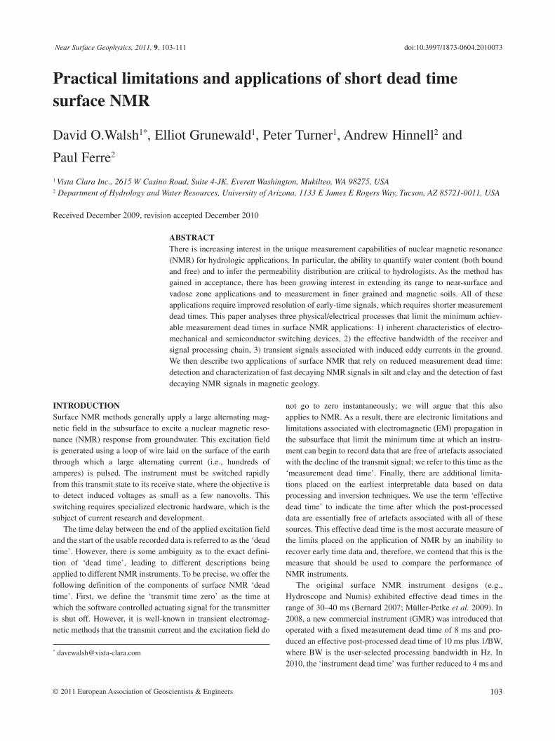
factor of the effective RLC circuit) of the coil when the transmit-ter is not engaged. This causes the voltage and current on the coil to dissipate in a controlled and reasonably rapid manner. This transmitter shut-off time is approximately 1 ms in most situa-tions and depends somewhat on the Q-factor of the tuned coil. An example of the GMR transmit waveform is shown in Fig. 1. In this example, the coil current and voltage are brought to zero within 0.7 ms of the end of the transmitter actuation sig-nal. This result is typical using single turn and 2-turn loops with diameters from 25–150 m. Hence, with the GMR instrument, the transmitter turn-off delay typically contributes around one mil-lisecond to the overall measurement dead time. A second category of hardware-related limitations to the dead time are delays and transients associated with switching from transmit to receive mode. The GMR utilizes electromechanical relays to isolate the receive circuitry from the transmitter during transmit mode. These devices have finite closing times, which add to the minimum measurement dead time. The present GMR software employs a conservative fixed switching delay of 4 ms between the end of an active transmit pulse and the closing of the receive relays.

Limitations related to bandwidthAnother fundamental limitation on the measurement dead time and/or the effective dead time is the bandwidth of the receive electronics and/or software filtering. The bandwidth of the receiver may be fixed in the hardware due to analogue filtering and/or due to parallel tuning of the loop in receive mode. A parallel-tuned receive loop exhibits a finite bandwidth of approximately f

o/Q, where fo is the resonant frequency of the coil

FIGURE 1

Illustration of transmitter shut-off time in the GMR instrument. This

example used a tuned 91 m square transmit loop. The transmitter is active

between t = –10 ms and t = 0 ms. The reduced Q-factor after t = 0 is

evidenced by the rapid decay of the coil current, compared with the

slower rise time at the start of the pulse.

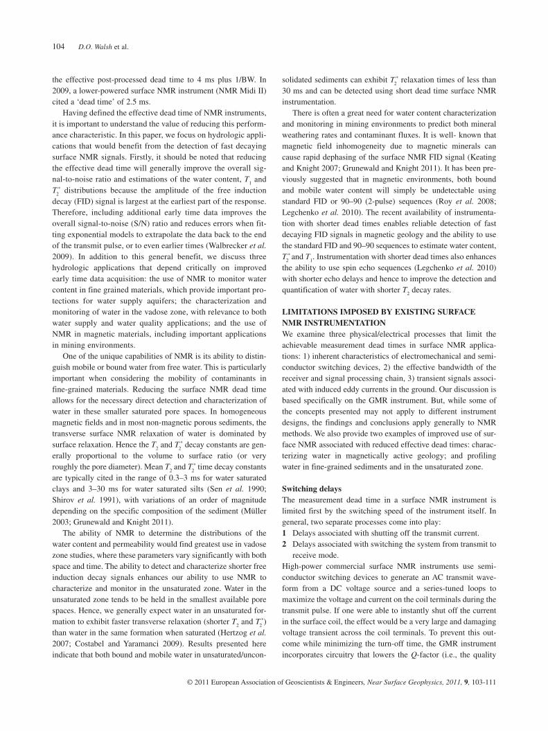
FIGURE 2

Three example signals showing dead time limitations related to the filter

bandwidth. The black lines show unfiltered exponential decays with

relaxation time constants of 5 ms, 15 ms and 45 ms. The coloured lines

show the signals after filtering using a Hanning window with a band-

width of 300 Hz. The filtered signals are coloured red for times

0 < t < 1/BW (0–3.3 ms), green for times 1/BW < t < 2/BW (3.3–6.6 ms)

and blue for times t > 2/BW (after 6.6 ms). The black circles reflect the

point at which each filtered signal turns concave up.



(0–3.3 ms), green for times 1/BW < t < 2/BW (3.3–6.6 ms) and blue for times t > 2/BW (after 6.6 ms). At times shorter than 1/BW, the filtered signal has much lower amplitude than the original unfiltered signal and is increasing monotonically in time. At a time of approximately 1/BW (3.3 ms) each filtered signal approaches its maximum and begins to decay, however, the time at which this maximum occurs varies somewhat depend-ing on the relaxation time constant. Immediately following the maximum, the filtered signal is rounded and concave down, unlike an exponential decay, until a point of inflection occurs (indicated by a black circle). After this inflection the signal becomes concave up and closely approximates the true unfiltered signal. For all three signals, this inflection point occurs very close to time t = 2/BW (~6.6 ms). Based on these examples, we suggest that a very conservative approach would exclude data at times shorter than t = 2/BW from the analysis. We note, however, that at time t = 1/BW the filtered signal has reached approximately 90% of its true value, suggest-ing that a more aggressive approach using a cut off time of t = 1/BW will likely result in only minor interpretation errors.

LIMITATIONS RELATED TO THE TRANSIENT EM RESPONSE OF THE GROUNDThe authors, among others, have in the past speculated on the potential for transient-EM induced eddy currents in the ground to obscure early time surface NMR signals. The argument goes that the surface NMR transmit pulse generates large values of dB/dt in the subsurface – larger in fact than many commer-cially available time-domain EM instruments can generate. Such large time-domain fluctuations of the magnetic field inevitably create eddy currents in an electrically-conductive earth and these eddy currents continue to flow and generate their own magnetic fields for some time after the termination of the surface NMR pulse. Computer modelling was performed to investigate the poten-tial for TEM-induced signals to interfere with short-time NMR signals. Computer simulations were performed using the Electro Magnetic Model Analysis (EMMA) software package (Aarhus Geophysics). The EMMA software package was used to model the vertical component of the transient magnetic field and its time derivative, generated by one cycle of a modelled surface NMR transmit pulse. The model assumed a circular single-turn transmit coil, a transmit frequency of 2.0 kHz and the field and field derivative was calculated at the centre of the transmit loop. All simulations assumed a uniform half-space resistivity, a peak transmit current of 400 A and the half-space resistivity and coil diameter were varied. The induced voltage on the transmit loop (i.e., coincident transmit/receive loop configuration) was estimated by assuming the induced field was uniform across the loop. This assumption is approximately valid in the late-time TEM response when the vertical depth of the propagating current filament (or ‘smoke ring’) is more than 3 times the diameter of the coil. The approx-

We illustrate this limitation related to the bandwidth in Fig. 2. In black we show three different signals prior to filtering with exponential relaxation times of 5 ms, 15 ms and 45 ms. Each signal is filtered using a Hanning window with a bandwidth of 300 Hz and the resulting filtered signals are shown in colour. The filtered signals are coloured red for times 0 < t < 1/BW

FIGURE 3

Left: simulation of TEM-induced voltage for a 50 m coil over a 100 Ωm

half-space, after zeroing the first 2 ms and filtering to a bandwidth of

400 Hz. Right: the same computer simulation result using a 50 m coil

over a 10 Ωm half-space, increasing the effective dead time from about

6 ms to about 9 ms.

FIGURE 4

Left: simulation of TEM-induced voltage for a 10 m diameter coil over a

40 Ωm half-space, after zeroing the first 2 ms and filtering to a bandwidth

of 400 Hz. Right: the same computer simulation result using a 150 m

diameter coil over a 40 Ωm half-space, increasing the effective dead time

from about 3 ms to about 10 ms.

FIGURE 5

Left: simulation of TEM-induced voltage for a 50 m diameter coil over a

10 Ωm half-space, after zeroing the first 2 ms and filtering to a bandwidth

of 400 Hz. Right: the same computer simulation but with the receive

switching time increased to 4 ms. In this simulation the longer switching

delay allows the TEM-induced energy to substantially decay prior to

‘closing’ the receive circuit and hence the effective dead time is actually

reduced from about 9 ms to about 7 ms.



In this paper we have not modelled the TEM-induced tran-sients with figure-eight coils. Intuitively, one would expect a figure-eight coil to be less susceptible to TEM-induced transients for two reasons. First the downward propagating current fila-ments from the two circles of figure-eight exhibit opposite cur-rent directions and hence their induced fields at the surface will tend to cancel as the currents filaments propagate downward and expand outward to the point where they nearly overlap. Second, the figure-eight coil in receive mode is insensitive to uniform vertical magnetic fields and as such it largely cancels the field from the downward propagating current filaments. These analyses demonstrate that transients associated with EM propagation in the subsurface are likely to place limits on the mini-mum achievable effective dead time. This impact will vary with the coil size and shape and the subsurface electrical properties. In general, the contributions to the effective dead time due to switching delays, finite bandwidth and transient effects are addi-tive. Thus, in the present data collection and processing scheme, the manufacturer cites an ‘instrument dead time’ of 4 ms and a minimum effective post-processed dead time of 4 ms + 1/BW, where BW is the processing bandwidth selected by the user dur-ing the post-processing stage.

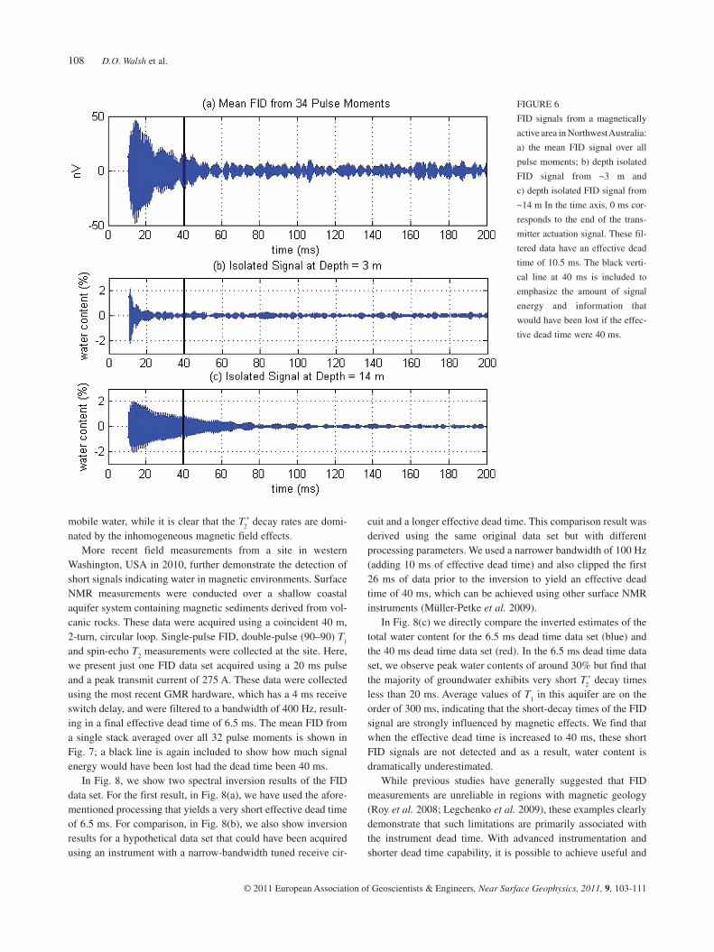
EXPERIMENTAL RESULTSDetection and characterization of groundwater in magnetic geologySurface NMR data were acquired in a region of Western Australia with widespread iron ore, using a GMR instrument with standard commercial software. Regional magnetic maps and ground based magnetometer surveys showed significant gradients in the static magnetic field at the survey site. A double-pulse (90–90) sequence was used to acquire surface NMR data. For the data presented here, we used a coincident 70 m square, single-turn transmit loop, with a maximum transmit current of 397 A, a transmit pulse length of 10 ms, an interpulse delay of 300 ms, a repetition delay of 6 s and 8 stacks of 34 pulse moments. In 2009 when these data were collected, the receive switching delay was 8 ms. These data were filtered to a bandwidth of 400 Hz, result-ing in a final effective dead time of 10.5 ms. The mean FID signal from the first pulse, averaged over all 34 pulse moments, is shown in Fig. 6(a). The black vertical bar in the time domain plot indicates where the processed data would have started if the effective dead time had been 40 ms. These data were processed using a linear 1D spatial inversion to isolate the NMR signals at discrete depth intervals followed by mono-exponential and multi-exponential fitting (Walsh 2008), which estimated the peak water content in the primary shallow frac-tured rock aquifer to be at least 7%. The NMR signals isolated at depths of 3 m (Fig. 6b) and 14 m (Fig. 6c) illustrate the range of T

2* decay rates produced by groundwater at this location. The

estimated mean T2* in this aquifer was approximately 20 ms,

while the estimated mean T1 in this aquifer ranged from 325–460 ms. These relatively long T1 decay rates are consistent with

imate downward velocity of the approximate current filament is given by

(1)

where σ is the half-space conductivity and υ is given in m/s (Ward and Hohmann 1988). The late-time TEM response of a conductive half-space to a step current in a surface loop is principally a non-oscillating power-law decay. The preprocessing of surface NMR data involves band-pass filtering the received signal to a band of a few hundred Hz around the Larmor frequency, which ranges from 1–3 kHz. So what really matters for surface NMR detec-tion is the transient response of the ground after switching delays and filtering. To simulate the effect of the TEM-induced voltage on the detected surface NMR signal, we processed the EMMA-modelled TEM data in the following steps. First the TEM data were inter-polated and re-sampled with a uniform sampling rate of 50 kHz. Next the initial portion of the TEM response was set to zero, for a period of 2–4 ms, to simulate the closing of receive switches at delays of 2–4 ms after the end of the transmit pulse. Finally the resultant data were digitally filtered, using a non-causal 10th order FIR Butterworth filter, to a bandwidth of 100–1000 Hz around the 2 kHz band of interest. This filtered TEM response was calculated using coil diameters from 10–150 m and for half-space resistivity values ranging from 1–1000 Ωm. The simulation results shown in Fig. 3 compare the modelled TEM-induced transients for a loop diameter of 50 m, a receive switching delay of 2 ms, a 400 Hz filter bandwidth and half-space resistivity values of 100 Ωm and 10 Ωm, respectively. If we set a detection threshold of 5 nV for the desired NMR signal, then these simulation results indicate that with a bandwidth of 400 Hz and receive switching time of 2 ms, the TEM response in the filtered data exceeds the detection threshold for the first 6 ms for a 100 Ωm half-space and the TEM response exceeds the detection threshold for the first 9 ms for a 10 Ωm half-space. The simulation results in Fig. 4 compare the TEM-induced transients for a 10 m diameter coil versus a 150 m diameter coil over the same 40 Ωm half-space. The amplitude of the induced voltage is expected to be proportional to d4, where d is the coil diameter. This is because the coil voltage is proportional to the area of the coil in receive mode and also the induced magnetic field and its time derivative are proportional to the area of the coil in the transmit mode (Ward and Hohmann 1988). The simulation results in Fig. 5 compare the TEM-induced transients for a 50 m diameter coil, over a 10 Ωm half-space, with the receive switching time set to 2 ms and 4 ms, respectively. This simulation indicates that in some cases it may be beneficial to delay the receive switching time to allow more time for the TEM-induced voltage on the coil to decay so that this energy does not enter the band-limited receive electronics and/or band-pass filter.



cuit and a longer effective dead time. This comparison result was derived using the same original data set but with different processing parameters. We used a narrower bandwidth of 100 Hz (adding 10 ms of effective dead time) and also clipped the first 26 ms of data prior to the inversion to yield an effective dead time of 40 ms, which can be achieved using other surface NMR instruments (Müller-Petke et al. 2009). In Fig. 8(c) we directly compare the inverted estimates of the total water content for the 6.5 ms dead time data set (blue) and the 40 ms dead time data set (red). In the 6.5 ms dead time data set, we observe peak water contents of around 30% but find that the majority of groundwater exhibits very short T2

* decay times less than 20 ms. Average values of T1 in this aquifer are on the order of 300 ms, indicating that the short-decay times of the FID signal are strongly influenced by magnetic effects. We find that when the effective dead time is increased to 40 ms, these short FID signals are not detected and as a result, water content is dramatically underestimated. While previous studies have generally suggested that FID measurements are unreliable in regions with magnetic geology (Roy et al. 2008; Legchenko et al. 2009), these examples clearly demonstrate that such limitations are primarily associated with the instrument dead time. With advanced instrumentation and shorter dead time capability, it is possible to achieve useful and

mobile water, while it is clear that the T2* decay rates are domi-

nated by the inhomogeneous magnetic field effects. More recent field measurements from a site in western Washington, USA in 2010, further demonstrate the detection of short signals indicating water in magnetic environments. Surface NMR measurements were conducted over a shallow coastal aquifer system containing magnetic sediments derived from vol-canic rocks. These data were acquired using a coincident 40 m, 2-turn, circular loop. Single-pulse FID, double-pulse (90–90) T1 and spin-echo T2 measurements were collected at the site. Here, we present just one FID data set acquired using a 20 ms pulse and a peak transmit current of 275 A. These data were collected using the most recent GMR hardware, which has a 4 ms receive switch delay, and were filtered to a bandwidth of 400 Hz, result-ing in a final effective dead time of 6.5 ms. The mean FID from a single stack averaged over all 32 pulse moments is shown in Fig. 7; a black line is again included to show how much signal energy would have been lost had the dead time been 40 ms. In Fig. 8, we show two spectral inversion results of the FID data set. For the first result, in Fig. 8(a), we have used the afore-mentioned processing that yields a very short effective dead time of 6.5 ms. For comparison, in Fig. 8(b), we also show inversion results for a hypothetical data set that could have been acquired using an instrument with a narrow-bandwidth tuned receive cir-

FIGURE 6

FID signals from a magnetically

active area in Northwest Australia:

a) the mean FID signal over all

pulse moments; b) depth isolated

FID signal from ~3 m and

c) depth isolated FID signal from

~14 m In the time axis, 0 ms cor-

responds to the end of the trans-

mitter actuation signal. These fil-

tered data have an effective dead

time of 10.5 ms. The black verti-

cal line at 40 ms is included to

emphasize the amount of signal

energy and information that

would have been lost if the effec-

tive dead time were 40 ms.



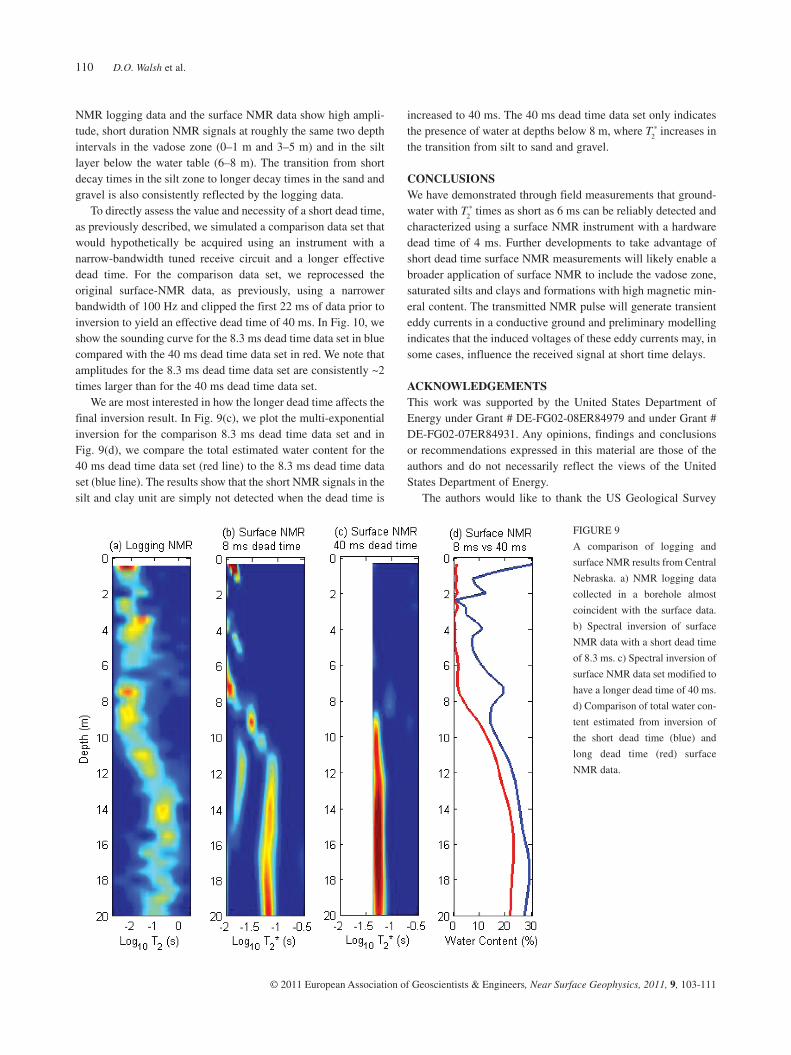
2010). This small-diameter NMR logging tool provides 0.5 m vertical resolution NMR measurements of the formation immediately surrounding a well or borehole in a 1D depth profile. The sensitive region of this tool is a cylindrical shell located approximately 19 mm radially from the tool centre. Logging data were acquired to a depth of 128 m in a 6 inch diameter well located coincident to the surface measurements. The logging tool was operated at a frequency of 250 kHz with an echo spacing of 2.5 ms, enabling quantification of water content with T2 relaxation constants on the order of 2 ms or longer. In Fig. 9 we show spectral inversion results for the NMR borehole logging data (Fig. 9a) and short dead time surface NMR data (Fig. 9b). In the vadose zone, the surface NMR data resolve strong signals with short T2

* (less than 20 ms) at depth intervals of 0–1 m and 3–4 m. The surface NMR data also resolve a strong signal from a silt layer in the saturated zone at a depth of 6–8 m. Deeper into the saturated zone, the surface NMR data indicate a transition between 8–12 m, over which T2

* gradually increases to ~100 ms in the deeper sand and gravel layers. The borehole NMR data provide an ideal ground-truth to evaluate the accuracy and reliability of the surface NMR data.

informative FID and T1 measurements of groundwater in mag-netic environments.

Application of short dead time to image vadose-zone and silt-bound waterVista Clara acquired a suite of surface NMR data in collaboration with the US Geological Survey in Central Nebraska, USA, dur-ing April 2009. This ongoing project has been supported by the Central Platte Natural Resource District (CPNRD), a regional government agency that manages groundwater in this agricul-tural region of the United States. The primary goal of the project is to develop and demonstrate methodologies for using surface NMR to improve regional groundwater models of the High Plains Aquifer system. For the collection of surface NMR data, we used a GMR instrument, which at the time had a receive switch delay of 5 ms; we again used standard processing and inversion software (Walsh 2008). In addition to large-loop surveys that investigate groundwater in the deep aquifer, we conducted a small loop survey at one site to investigate the vadose zone and a shallower aquifer. Driller’s logs and other geophysical logs from this site describe the upper 10 m of sediments as interbedded layers of silt and clay, underlain by sands and gravels at depths of 10–21 m. The depth of the water table was approximately 5 m. Single-pulse (FID) data were acquired at the site using a small loop with a transmit pulse length of 10 ms. A single-turn diamond-eight loop with a side dimension of 45 m was used to both transmit and receive. Two other coils were used for adaptive noise cancellation (Walsh 2008). To maximize sensitivity to short signals, the FID data were processed using a filter bandwidth of 300 Hz, resulting in an effective post-processed dead time of 8.3 ms. In addition to the 2009 surface NMR data, Vista Clara also acquired borehole NMR logging data at the site in 2010 using the newly developed Javelin tool (Vista Clara Inc., Mukilteo Washington, USA) (Walsh et al.

FIGURE 7

The FID signal from a coastal aquifer in Western Washington containing

magnetic sediments. Shown is the mean FID averaged over all 32 pulse

moments for a single stack. In the time axis, 0 ms corresponds to the end

of the transmitter actuation signal. These data have an effective dead time

of 6.5 ms. The black vertical line at 40 ms is included to emphasize the

amount of signal energy and information that would have been lost if the

effective dead time was 40 ms.

FIGURE 8

Comparison of spectral inversions and estimate water content from a

coastal aquifer in western Washington, USA containing magnetic sedi-

ments. a) Data set processed with effective dead time of 6.5 ms. b) Data

set processed with effective dead time of 40 ms. c) Comparison of

derived total water content for the 6.5 ms dead time (blue) and 40 ms

dead time (red) data sets.



increased to 40 ms. The 40 ms dead time data set only indicates the presence of water at depths below 8 m, where T2

* increases in the transition from silt to sand and gravel.

CONCLUSIONSWe have demonstrated through field measurements that ground-water with T2

* times as short as 6 ms can be reliably detected and characterized using a surface NMR instrument with a hardware dead time of 4 ms. Further developments to take advantage of short dead time surface NMR measurements will likely enable a broader application of surface NMR to include the vadose zone, saturated silts and clays and formations with high magnetic min-eral content. The transmitted NMR pulse will generate transient eddy currents in a conductive ground and preliminary modelling indicates that the induced voltages of these eddy currents may, in some cases, influence the received signal at short time delays.

ACKNOWLEDGEMENTSThis work was supported by the United States Department of Energy under Grant # DE-FG02-08ER84979 and under Grant # DE-FG02-07ER84931. Any opinions, findings and conclusions or recommendations expressed in this material are those of the authors and do not necessarily reflect the views of the United States Department of Energy. The authors would like to thank the US Geological Survey

NMR logging data and the surface NMR data show high ampli-tude, short duration NMR signals at roughly the same two depth intervals in the vadose zone (0–1 m and 3–5 m) and in the silt layer below the water table (6–8 m). The transition from short decay times in the silt zone to longer decay times in the sand and gravel is also consistently reflected by the logging data. To directly assess the value and necessity of a short dead time, as previously described, we simulated a comparison data set that would hypothetically be acquired using an instrument with a narrow-bandwidth tuned receive circuit and a longer effective dead time. For the comparison data set, we reprocessed the original surface-NMR data, as previously, using a narrower bandwidth of 100 Hz and clipped the first 22 ms of data prior to inversion to yield an effective dead time of 40 ms. In Fig. 10, we show the sounding curve for the 8.3 ms dead time data set in blue compared with the 40 ms dead time data set in red. We note that amplitudes for the 8.3 ms dead time data set are consistently ~2 times larger than for the 40 ms dead time data set. We are most interested in how the longer dead time affects the final inversion result. In Fig. 9(c), we plot the multi-exponential inversion for the comparison 8.3 ms dead time data set and in Fig. 9(d), we compare the total estimated water content for the 40 ms dead time data set (red line) to the 8.3 ms dead time data set (blue line). The results show that the short NMR signals in the silt and clay unit are simply not detected when the dead time is

FIGURE 9

A comparison of logging and

surface NMR results from Central

Nebraska. a) NMR logging data

collected in a borehole almost

coincident with the surface data.

b) Spectral inversion of surface

NMR data with a short dead time

of 8.3 ms. c) Spectral inversion of

surface NMR data set modified to

have a longer dead time of 40 ms.

d) Comparison of total water con-

tent estimated from inversion of

the short dead time (blue) and

long dead time (red) surface

NMR data.



Keating K. and Knight R. 2007. A laboratory study to determine the effect of iron oxides on proton NMR measurements. Geophysics 72, E27–E32.

Legchenko A., Vouillamoz J.-M. and Roy J. 2010. Application of the magnetic resonance method to the investigation of aquifers in the pres-ence of magnetic materials. Geophysics 75, L91. doi:10.1190/1.3494596

Müller M. 2003. Dispersion of nuclear magnetic resonance (NMR) relaxation. 20th Kolloquium Electromagnetische Tiefenforschung, 29 September–3 October 2003, Konigstien, Switzerland, Expanded Abstracts.

Müller-Petke M., Costabel S., Lange G. and Yaramanci U. 2009. Assessment of improved measurement technology for magnetic reso-nance sounding. 4th International Workshop on Magnetic Resonance Sounding, 20–23 October 2009, Grenoble, France, Expanded Abstracts, 153–158.

Nilsson J.W. 1986. Electric Circuits. Addison-Wesley.Roy J., Rouleau A., Chouteau M. and Bureau M. 2008. Widespread

occurrence of aquifers currently undetectable with the MRS technique in the Grenville geological province, Canada. Journal of Applied Geophysics 66, 82–93.

Sen P.N., Straley C., Kenyon W.E. and Whittingham M.S. 1990. Surface to volume ratio, charge density, nuclear magnetic relaxation and per-meability in clay bearing sandstones. Geophysics 55, 61–69.

Shirov M., Legchenko A. and Creer G. 1991. A new direct non-invasive groundwater detection technology for Australia. Exploration Geophysics 22, 333–338.

Walbrecker J.O., Hertrich M. and Green A.G. 2009. Accounting for relaxation processes during the pulse in surface NMR data. Geophysics 74, G27. doi:10.1190/1.3238366

Walsh D.O. 2008. Multi-channel surface NMR instrumentation and soft-ware for 1D/2D groundwater investigations. Journal of Applied Geophysics 66, 140–150.

Walsh D.O., Grunewald E., Turner P. and Frid I. 2010. Javelin: A slim-hole and microhole NMR logging tool. Fast Times 15(3), 67–72.

Ward S.H. and Hohmann G.W. 1988. Electromagnetic theory for geo-physical applications. In: Electromagnetic Methods in Applied Geophysics, 1 (ed. M.N. Nabighian), 131–311. SEG.

and the Central Platte Natural Resources District for their per-mission to use the surface NMR data from Nebraska, USA.. The authors would also like to thank GroundProbe Ltd Pty and Rio Tinto for their permission to use the surface NMR data from Western Australia. The authors finally would like to thank the Washington Department of Fish and Wildlife for their permission to use the surface NMR data from western Washington, USA.

REFERENCESAuken E., Nebel L., Sorensen K., Breiner M., Pellerin L. and Christensen

N.B. 2002. EMMA – A geophysical training and education tool for electromagnetic modeling and analysis. Journal of Environmental and Engineering Geophysics 7, 57–68.

Bernard J. 2007. Instruments and field work to measure a magnetic reso-nance sounding. Boletin Geologico y Minero 118, 459–472.

Costabel S. and Yaramanci U. 2009. Potential of Earth’s field NMR (EFNMR) to characterize the vadose zone. 4th International Workshop on Magnetic Resonance Sounding, 20–23 October 2009, Grenoble, France, Expanded Abstracts, 41–46.

Grunewald E. and Knight R. 2011. The effect of pore size and magnetic susceptibility on the surface NMR relaxation parameter T2

*. Near Surface Geophysics 9 (this issue).

Hertzog R.C., White T.A. and Straley C. 2007. Using NMR decay-time measurements to monitor and characterize DNAPL and moisture in sub surface porous media. Journal of Environmental and Engineering Geophysics 12, 293–306.

FIGURE 10

A comparison of the sounding curves for the 8.3 ms dead time data set

(blue) and 40 ms dead time comparison data set (red).

Documents

Practical limitations and applications of short dead …vista-clara.com/wp-content/uploads/2012/11/Walsh-et-al-2011-short... · Practical limitations and applications of short dead