1

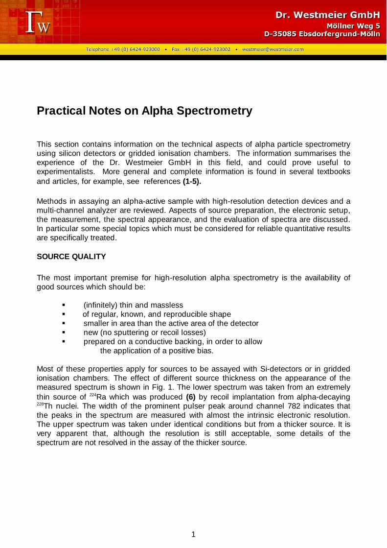
Practical Notes on Alpha Spectrometry This section contains information on the technical aspects of alpha particle spectrometry using silicon detectors or gridded ionisation chambers. The information summarises the experience of the Dr. Westmeier GmbH in this field, and could prove useful to experimentalists. More general and complete information is found in several textbooks and articles, for example, see references (1-5). Methods in assaying an alpha-active sample with high-resolution detection devices and a multi-channel analyzer are reviewed. Aspects of source preparation, the electronic setup, the measurement, the spectral appearance, and the evaluation of spectra are discussed. In particular some special topics which must be considered for reliable quantitative results are specifically treated. SOURCE QUALITY

The most important premise for high-resolution alpha spectrometry is the availability of good sources which should be: � (infinitely) thin and massless � of regular, known, and reproducible shape � smaller in area than the active area of the detector � new (no sputtering or recoil losses) � prepared on a conductive backing, in order to allow the application of a positive bias. Most of these properties apply for sources to be assayed with Si-detectors or in gridded ionisation chambers. The effect of different source thickness on the appearance of the measured spectrum is shown in Fig. 1. The lower spectrum was taken from an extremely thin source of 224Ra which was produced (6) by recoil implantation from alpha-decaying 228Th nuclei. The width of the prominent pulser peak around channel 782 indicates that the peaks in the spectrum are measured with almost the intrinsic electronic resolution. The upper spectrum was taken under identical conditions but from a thicker source. It is very apparent that, although the resolution is still acceptable, some details of the spectrum are not resolved in the assay of the thicker source.

2

Figure 1: Alpha spectra measured from an extremely thin recoil implanted source of 224Ra and from a somewhat thicker source. The small peak around channel 782 is from a pulser. ELECTRONIC SETUP

A block diagram of a typical setup for alpha-particle spectrometry (7) is shown in Fig. 2. It will be generally discussed in two parts: the detectors and the linear electronics for signal processing. Detectors The leftmost part of the figure could contain any appropriate type of detector such as: Surface Barrier Detector (SBD) This relatively cheap detector which is an article of consumption with a sensitive surface of up to 20 cm2 is an ideal device for simple and fast setups where small sources are to be assayed with good resolution. Depending on the size of the detector, the resolution of a small unit may be as good as 12 keV FWHM for 5.5 MeV alpha-particles. The resolution of very large SBDs will be around 40-50 keV FWHM. The bias voltage applied to SBD is usually in the range of 40 to 100 Volts where the polarity may be either positive or negative, depending on the type of the detector; it is therefore always best to check the manual for the correct voltage and polarity before applying the bias voltage! Also, most types of SBD must not be exposed to any light when the bias voltage is applied because they are sensitive to light and they will measure excessive noise in the low energy regime. There are ruggedized SBD available where the front electrode is covered with a thin aluminum (-oxide) layer which can be gently washed with appropriate agents. One must avoid any force to the surface of a SBD unit during the cleaning operation or else. SBDs which are handled with reasonable care will last about 1*108 to 5*108 impinging alpha particles or 1*107 to 5*107 fission fragments. The energetic particles will damage the

3

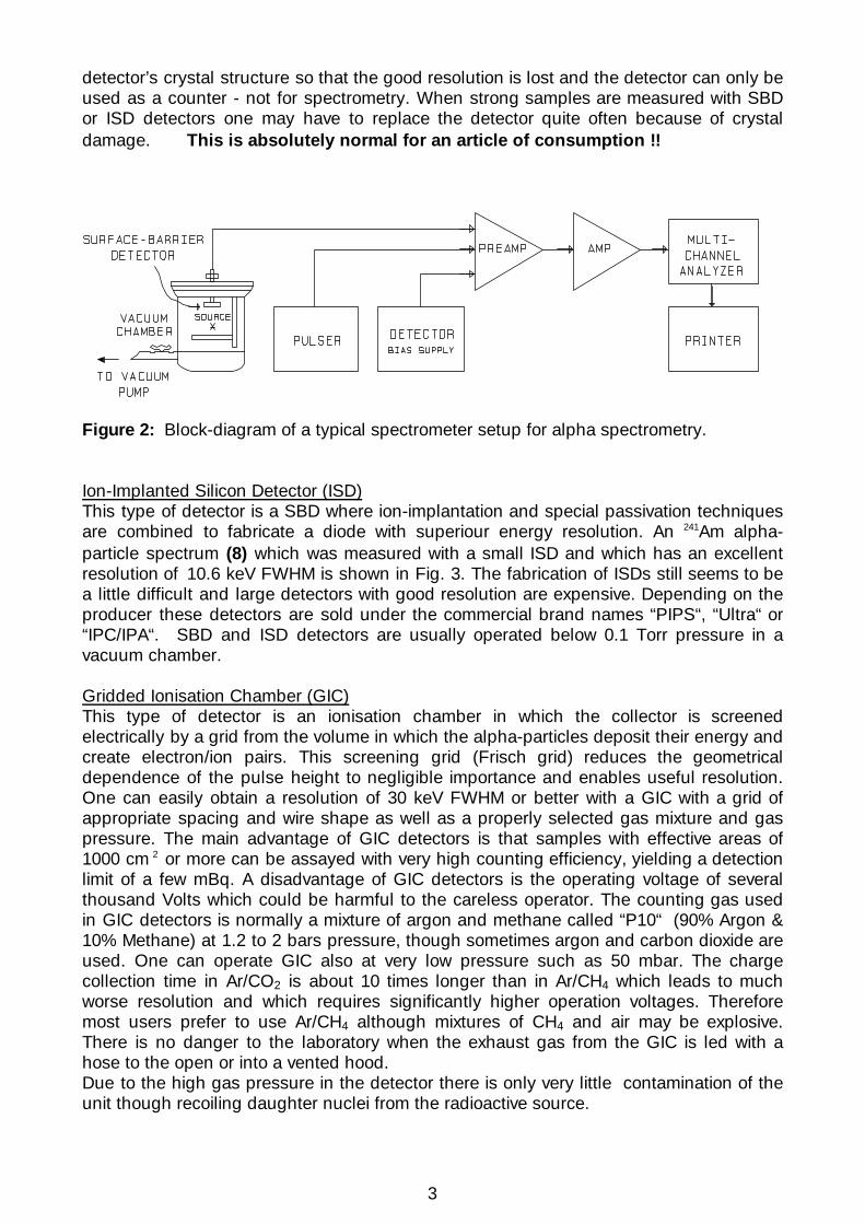
detector’s crystal structure so that the good resolution is lost and the detector can only be used as a counter - not for spectrometry. When strong samples are measured with SBD or ISD detectors one may have to replace the detector quite often because of crystal damage. This is absolutely normal for an article of consumption !!

Figure 2: Block-diagram of a typical spectrometer setup for alpha spectrometry. Ion-Implanted Silicon Detector (ISD) This type of detector is a SBD where ion-implantation and special passivation techniques are combined to fabricate a diode with superiour energy resolution. An 241Am alpha-particle spectrum (8) which was measured with a small ISD and which has an excellent resolution of 10.6 keV FWHM is shown in Fig. 3. The fabrication of ISDs still seems to be a little difficult and large detectors with good resolution are expensive. Depending on the producer these detectors are sold under the commercial brand names “PIPS“, “Ultra“ or “IPC/IPA“. SBD and ISD detectors are usually operated below 0.1 Torr pressure in a vacuum chamber. Gridded Ionisation Chamber (GIC) This type of detector is an ionisation chamber in which the collector is screened electrically by a grid from the volume in which the alpha-particles deposit their energy and create electron/ion pairs. This screening grid (Frisch grid) reduces the geometrical dependence of the pulse height to negligible importance and enables useful resolution. One can easily obtain a resolution of 30 keV FWHM or better with a GIC with a grid of appropriate spacing and wire shape as well as a properly selected gas mixture and gas pressure. The main advantage of GIC detectors is that samples with effective areas of 1000 cm 2

or more can be assayed with very high counting efficiency, yielding a detection limit of a few mBq. A disadvantage of GIC detectors is the operating voltage of several thousand Volts which could be harmful to the careless operator. The counting gas used in GIC detectors is normally a mixture of argon and methane called “P10“ (90% Argon & 10% Methane) at 1.2 to 2 bars pressure, though sometimes argon and carbon dioxide are used. One can operate GIC also at very low pressure such as 50 mbar. The charge collection time in Ar/CO2 is about 10 times longer than in Ar/CH4 which leads to much worse resolution and which requires significantly higher operation voltages. Therefore most users prefer to use Ar/CH4 although mixtures of CH4 and air may be explosive. There is no danger to the laboratory when the exhaust gas from the GIC is led with a hose to the open or into a vented hood. Due to the high gas pressure in the detector there is only very little contamination of the unit though recoiling daughter nuclei from the radioactive source.

4

There are other devices which may be used for the detection and spectrometry of alpha particles, but these will not be discussed within the context of this paper. All detectors mentioned above are operated at room temperature; cooling the detectors to an easily obtained -35oC brings a negligible enhancement in the resolution and no improvement in the efficiency. Analog Signal Processing The detector signal is fed into a pre-amplifier (see Fig. 2) where also the detector bias supply is connected. In order to reduce electronic noise and to improve resolution, the cable from the detector to the pre-amplifier should be as short as possible and well shielded. The pre-amplifier should be selected so as to match with the capacitance of the detector. The output signal from the pre-amplifier is fed via a shielded cable into a linear amplifier which has appropriate shaping and baseline restoration circuitry. Biased amplifiers are most frequently used in alpha spectrometry where the alpha energy range from 0 to 3 or 4 MeV is electronically suppressed. This feature serves for the suppression of electronic noise and beta particles and it allows measurement in the relevant energy

Figure 3: Spectrum of a 241Am alpha-particle source measured with an ISD detector (log scale). range from 4 to 9 MeV with suitable amplification. (There are only very few cases where alpha-particle energies below 4 MeV or above 9 MeV are of interest: out of the ca. 1900 known alpha lines from 592 nuclides (9) there are only 105 lines below 4 MeV and 64 lines above 9 MeV.) The unipolar output of the amplifier which is fed into the ADC input of the multichannel analyser system must have properly adjusted pole-zero cancellation, a shaping time of 4 µs or above, and a DC level which matches the ADC input level to within 10 mV. The connection is made with a well shielded 50 Ohms coaxial cable. If a long distance of 50 cm or more between the detector and the ADC input cannot be avoided then the only long cable should be connected from the pre-amplifier to the linear amplifier. A 12 % degradation of the resolution was measured when the pre-amplifier output signal was fed over 60 m of doubly shielded coaxial cable to the linear amplifier;

5

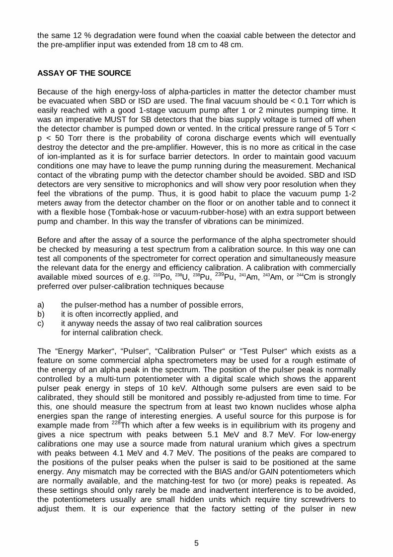
the same 12 % degradation were found when the coaxial cable between the detector and the pre-amplifier input was extended from 18 cm to 48 cm. ASSAY OF THE SOURCE Because of the high energy-loss of alpha-particles in matter the detector chamber must be evacuated when SBD or ISD are used. The final vacuum should be < 0.1 Torr which is easily reached with a good 1-stage vacuum pump after 1 or 2 minutes pumping time. It was an imperative MUST for SB detectors that the bias supply voltage is turned off when the detector chamber is pumped down or vented. In the critical pressure range of 5 Torr < p < 50 Torr there is the probability of corona discharge events which will eventually destroy the detector and the pre-amplifier. However, this is no more as critical in the case of ion-implanted as it is for surface barrier detectors. In order to maintain good vacuum conditions one may have to leave the pump running during the measurement. Mechanical contact of the vibrating pump with the detector chamber should be avoided. SBD and ISD detectors are very sensitive to microphonics and will show very poor resolution when they feel the vibrations of the pump. Thus, it is good habit to place the vacuum pump 1-2 meters away from the detector chamber on the floor or on another table and to connect it with a flexible hose (Tombak-hose or vacuum-rubber-hose) with an extra support between pump and chamber. In this way the transfer of vibrations can be minimized. Before and after the assay of a source the performance of the alpha spectrometer should be checked by measuring a test spectrum from a calibration source. In this way one can test all components of the spectrometer for correct operation and simultaneously measure the relevant data for the energy and efficiency calibration. A calibration with commercially available mixed sources of e.g. 210Po, 238U, 238Pu, 239Pu, 241Am, 243Am, or 244Cm is strongly preferred over pulser-calibration techniques because a) the pulser-method has a number of possible errors, b) it is often incorrectly applied, and c) it anyway needs the assay of two real calibration sources for internal calibration check. The “Energy Marker“, “Pulser“, “Calibration Pulser“ or “Test Pulser“ which exists as a feature on some commercial alpha spectrometers may be used for a rough estimate of the energy of an alpha peak in the spectrum. The position of the pulser peak is normally controlled by a multi-turn potentiometer with a digital scale which shows the apparent pulser peak energy in steps of 10 keV. Although some pulsers are even said to be calibrated, they should still be monitored and possibly re-adjusted from time to time. For this, one should measure the spectrum from at least two known nuclides whose alpha energies span the range of interesting energies. A useful source for this purpose is for example made from 228Th which after a few weeks is in equilibrium with its progeny and gives a nice spectrum with peaks between 5.1 MeV and 8.7 MeV. For low-energy calibrations one may use a source made from natural uranium which gives a spectrum with peaks between 4.1 MeV and 4.7 MeV. The positions of the peaks are compared to the positions of the pulser peaks when the pulser is said to be positioned at the same energy. Any mismatch may be corrected with the BIAS and/or GAIN potentiometers which are normally available, and the matching-test for two (or more) peaks is repeated. As these settings should only rarely be made and inadvertent interference is to be avoided, the potentiometers usually are small hidden units which require tiny screwdrivers to adjust them. It is our experience that the factory setting of the pulser in new

6

spectrometers is quite reliable and that one has to test the settings only once a year or after every new installation or repair. The distance to be chosen between the source and the detector is selected as a compromise between several constraints: � the count rate of the system should not exceed 400 - 500 Hz; if the count rate is higher than 1 kHz one definitely has to increase the distance between the source and the detector or to dilute the source � for very weak sources one may want to minimize the distance between the source and detector in order to maximize the geometrical efficiency � a very good resolution is only achieved when the distance between source and detector is large (> 2 * detector diameter) because then the alpha-particles traverse the dead layer on the detector surface almost perpendicular with minimal energy loss. Large distances, however, require also improved vacuum conditions and longer counting times � if a positive bias voltage is to be applied to the source as in specially designed chambers, in order to prevent conversion electrons and alpha recoils from reaching the detector, one should consider at least 1 mm distance per 100V bias. The "standard" setup of a weak source in front of a SBD or ISD without bias voltage to the source usually has more than 5 mm distance between the source and the detector surface. Out of these, ca. 1.5 mm is the unavoidable distance between the detector surface and the front end of the detector housing and the remaining 3.5 mm are caused by a poor construction of the source holder (even in commercially available systems!). The sample holder in alpha spectrometers should really be built in such a way that the source-to-detector distance can be continuously controlled and monitored at low distances. When the source distance is larger than 10 mm the typical sample holder shelf system is a good solution. The preferrably circular sources should be positioned under the detector (which is usually also circular) in such a way that source and detector surfaces are parallel with each other and the centers are axially aligned. For this setup one can easily calculate the geometrical opening angle from the source to the detector which defines the counting efficiency of the setup (see below). The dynamic energy range which is needed for the measurement of spectra of alpha-particles from radioactive decay usually covers ca. 5 MeV and it goes from 4 MeV to 9 MeV. Considering that the electronic resolution of a good detector usually is 15 keV FWHM or more, and that the total resolution will be even worse due to the finite thickness of the source, it is absolutely adequate and sufficient, to measure alpha-particle spectra of 1024 channels (1k) length. When a 5 MeV energy range is displayed on 1k channels, one channel is ca. 5 keV wide, i.e. the resolution (FWHM) of extremely well resolved peaks is 3 channels or above. A full width at half maximum of 3 channels is absolutely sufficient for any type of least-squares or other fitting procedure in the analysis of spectra and the measured data are easily analysed. The stretching of the spectrum on 2k or even 4k channels will not result in an improved ability to resolve close-lying multiplets or shoulder peaks. It will only enhance the amount of storage memory and evaluation time needed and it will make the statistical uncertainties worse. In fact, when the numbers of counts in a channel are low and their statistical uncertainties are therefore relatively large it may be impossible to discriminate a small low energy shoulder peak because it is statistically insignificant.

7

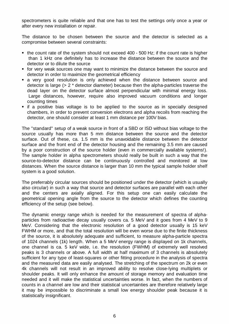
To show the effect of vacuum, bias voltage and source-to-detector distance Fig. 4 shows spectra measured with the same spectrometer from the same 241Am source, but under very different conditions. The spectra were measured with a normal linear amplifier without an energy bias, i.e. channel zero corresponds to approximately zero keV. The distributions found in alpha spectra at low energies (below channel 80 in Fig. 4) are either electronic noise counts or they may originate from negatrons, i.e. negatively charged beta particles, emitted from the source. All spectra shown in Fig. 4 were measured with a SBD with has a resolution of ca. 40 keV (FWHM). In the first spectrum the alpha distribution is a narrow peak around channel 680. The 241Am source was measured at close geometry, in moderate vacuum and with the recommended detector bias of -75V.

Figure 4: Alpha-particle spectra from 241Am measured with a SBD from the same source but under different conditions. For details, see text. The position of the main peak in channel 680 corresponds to an energy of 5485.6 MeV. In the second measurement (middle peak) the detector chamber was vented to normal pressure, the detector bias was switched off, and the source was again at 7 mm distance. There is still some appreciable response of the detector yielding a broader peak at channel 560 which corresponds to ca. 4.6 MeV. However, much more important than the loss in energy and resolution is the low energy noise contribution which is cut off in Fig. 4 at 2000 counts per channel and which peaks at over 2 million counts in one channel. The multichannel analyzer deadtime in this measurement without detector bias turned on was ca. 45 %. The third measurement (left peak) was made with the bias switched on, but at a large distance between source and detector and in a vented chamber. The resulting distribution is situated at an even lower energy and it contains only very few counts because the geometric efficiency for the larger distance is reduced by a factor of 6.6. Almost the same factor (6.3) is found in the ratio of peak-areas. The three spectra from Fig. 4 were measured for the same livetime of 102 seconds each. From the examples

8

shown in Fig. 4 it is clear that the proper operation of an alpha-particle spectrometer cannot be verified when only a few counts are visible in about the expected spectral range for the actual source. There are events measured even when the setting of the spectrometer is grossly mistaken. Instead, one has to measure the spectrum long enough until a well-defined peak is accumulated (peakheight > 1000 counts) and one must check the resolution of the setup. A fast resolution-check procedure that yields sufficiently good values for setup purposes is to interpolate at the high-energy (right) flank of the peak for the half-height channel. Twice the distance between the half-height channel and the center channel is about equal to the resolution (FWHM) in units of channels.

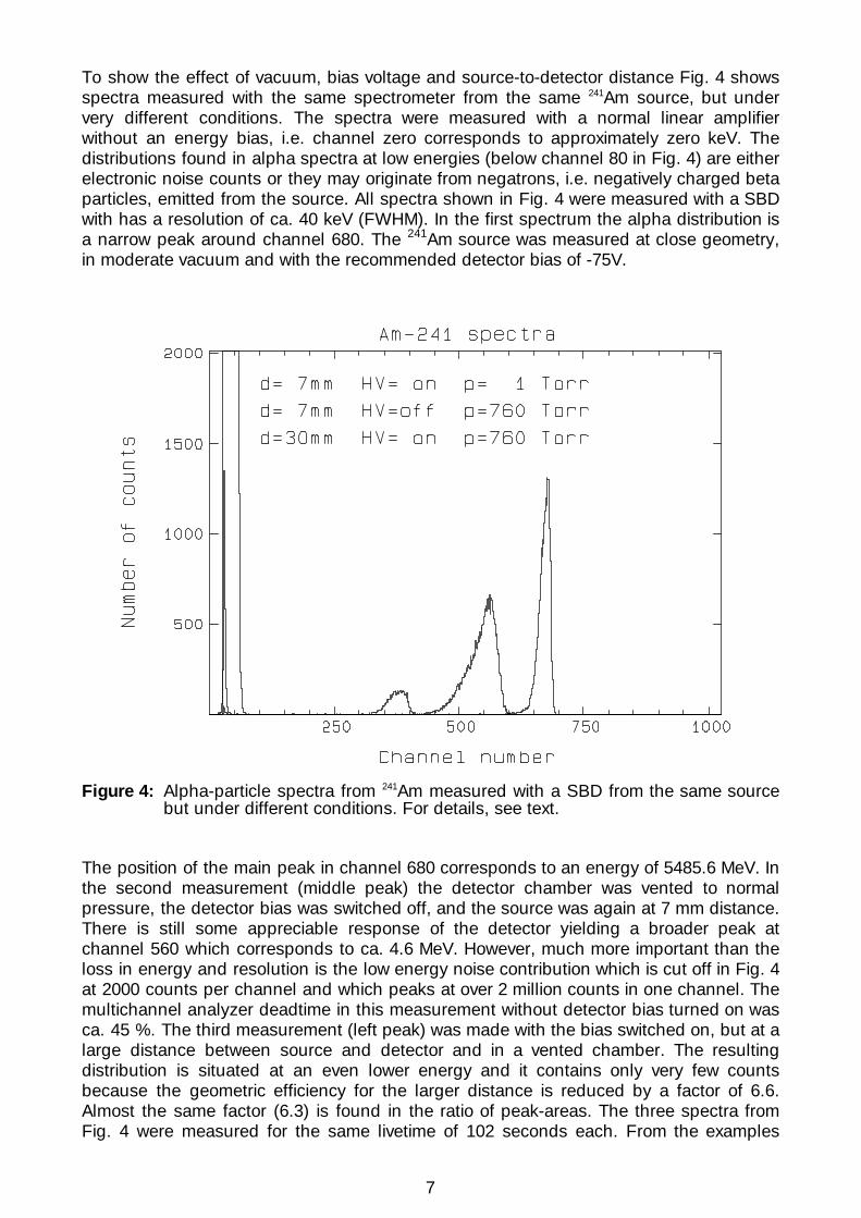
Figure 5: GIC alpha-particle spectrum from a thin mixed calibration source containing 239Pu, 241Am, and 244Cm. In Figs. 5 and 6 two sample spectra are shown which were measured with a gridded ionisation chamber. (10) The spectrum from Fig. 5 was measured from an essentially massless mixed calibration source and it exhibits peaks with very good resolution which sit on an almost constant background at ca. 0.1 % of the peakheight. This background is a typical property of alpha spectra in GIC and it comes from alpha-particles which deposited part of their energy in interactions with other material such as the chamber walls, grid wires or sample holder. In GIC detectors, this background is also from normal interactions where some fraction of the electrons from the ionisation process are lost through recombination or interaction with the grid. These events with incomplete energy deposition lead to a background distribution which under a peak or multiplet resembles very much the baseline distribution known from high-resolution gamma-ray spectrometry.

9

Figure 6: GIC alpha-particle spectrum from a very thick source. In contrast to the well resolved peaks from Fig. 5, the spectrum in Fig. 6 shows an almost unresolved distribution that decreases from the low-energy noise region over some intermediate structure down to "no counts" at high channel numbers. The spectrum shown in Fig. 6 was measured with a GIC from a thin layer of powdered granite rock which was milled to particles of 0.045 mm diameter or less. The energy loss of alpha-particles traversing through these thick granules is very large and consequently a low-energy tailing structure to the peaks is encountered which extends down to zero energy. ANALYSIS OF SPECTRA The quantitative analysis of alpha-particle spectra is aimed at the determination of the positions of peaks in units of channel numbers and of the areas of peaks in units of counts. Both quantities must be determined together with the associated uncertainties of these values. Using the energy- and efficiency-calibration data, the timing information from the measurement, and a nuclides library, these positions and areas are then converted into absolute activities of nuclides contained in the source. Simple analysis procedures

The analysis of high-activity-level alpha particle spectra from separated single-nuclide sources or of very-low-activity-level alpha spectra often does not require any sophisticated computerized procedures. In some of these cases it is sufficient to add up the number of counts in a preset window in order to get the area of the respective peak or peaks. The first momentum of the distribution of counts per channel is an approximation to the peak position which normally

10

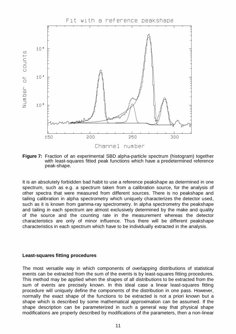
is good enough to check that this is really the peak of the expected nuclide. The method of extracting the positions of the peaks by the first momentum is restricted to the analysis of very simple spectra with only well-separated peaks. Whenever one has to analyze more complex spectra with overlapping peaks, where the number of peaks and their positions are not a priori known, these counting procedures cannot be applied. For the analysis of multiplet peaks which have resolved maxima, it appears to be a very poor approximation that the total number of counts in a sufficiently wide window be divided up according to the ratios of the heights of the individual peak maxima. Stripping methods which were once used for the resolution of NaI(Tl) gamma-ray spectra are also inapplicable to complex alpha particle spectra. Large peaks with well-resolved maxima may be extracted with reasonable accuracy, but the remaining distribution of counts per channel then is additionally scattered by the statistical fluctuations from the subtracted large peaks. These fluctuations cannot be accounted for when a predetermined reference function is subtracted. Moreover, one cannot assume a reference peakshape in an alpha spectrum which is generally usable for stripping or unfolding (see below). Consequently, there is no possibility to analyze small peaks in the vicinity of large ones by stripping methods. The principle of spectrum stripping is sometimes reversed in such a way that the measured spectrum is iteratively unfolded with a reference alpha peak function, where the positions and relative peak heights of the unfolded peaks are allowed to vary. Applying least-squares criteria for the fit between the measured spectrum and the calculated one, and minimizing the number of unfolded components in the resolved spectrum, one approaches the situation where a spectrum is simultaneously least-squares stripped from all peaks. When using this method of reference-peak definition one has to be aware of several implicit problems which will lead to large errors especially for minor peaks in the spectrum. The high-resolution 224Ra spectrum from Fig. 1 can be used as an example to visualize these implicit errors. The reference peakshape function was determined by a least-squares fit to the peak in channel 532 (see Fig. 1) where a minor contribution in channel 543 was also considered. Then this reference peakshape was used (FWHM and tailing shape fixed) to least-squares fit the positions and heights of peaks in the multiplet around channels 200 to 300. The result is shown in Fig. 7 where the original spectrum is plotted as a histogram and the fitted peaks as smooth lines. The baseline under the peaks is the analytical background distribution.(11) It is an apparent conclusion from Fig. 7 that the fitting of a pre-determined peakshape function to other peaks in the same spectrum but at different energies is absolutely inadequate. The FWHM of the reference peak in this example is considerably larger than the width of the peaks in Fig. 7 and consequently the least-squares fitting procedure misadjusted all peak-heights (and areas) and it was unable to reproduce the distribution around channel 290 as a multiplet peak. The fitting of a reference peakfunction to other peaks in the same spectrum may be applied for overview purposes, but it should be avoided when quantitative analyses are required.

11

Figure 7: Fraction of an experimental SBD alpha-particle spectrum (histogram) together with least-squares fitted peak functions which have a predetermined reference peak-shape. It is an absolutely forbidden bad habit to use a reference peakshape as determined in one spectrum, such as e.g. a spectrum taken from a calibration source, for the analysis of other spectra that were measured from different sources. There is no peakshape and tailing calibration in alpha spectrometry which uniquely characterizes the detector used, such as it is known from gamma-ray spectrometry. In alpha spectrometry the peakshape and tailing in each spectrum are almost exclusively determined by the make and quality of the source and the counting rate in the measurement whereas the detector characteristics are only of minor influence. Thus there will be different peakshape characteristics in each spectrum which have to be individually extracted in the analysis. Least-squares fitting procedures

The most versatile way in which components of overlapping distributions of statistical events can be extracted from the sum of the events is by least-squares fitting procedures. This method may be applied when the shapes of all distributions to be extracted from the sum of events are precisely known. In this ideal case a linear least-squares fitting procedure will uniquely define the components of the distribution in one pass. However, normally the exact shape of the functions to be extracted is not a priori known but a shape which is described by some mathematical approximation can be assumed. If the shape description can be parameterized in such a general way that physical shape modifications are properly described by modifications of the parameters, then a non-linear

12

least-squares fitting procedure can iteratively approximate the parameters to match the measured peakshapes and the components are found. The only premise for the applicability of such least-squares fitting procedures is the knowledge about a suitable shape function for alpha peaks and also for the baseline underlying the peaks. A general statement has been published for the peak shape of an alpha peak, (12,13) in which it is assumed that a single-energy delta function can be used with an exponential low-energy tail. The folding integral of this distribution with the Gaussian response function for the detector and electronics leads to the equation:

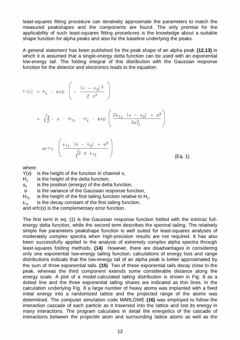
(Eq. 1) where Y(x) is the height of the function in channel x, H1 is the height of the delta function, x0 is the position (energy) of the delta function, σ is the variance of the Gaussian response function, HT1 is the height of the first tailing function relative to H1, εT1 is the decay constant of the first tailing function, and erfc(x) is the complementary error function. The first term in eq. (1) is the Gaussian response function folded with the intrinsic full-energy delta function, while the second term describes the spectral tailing. The relatively simple five parameters peakshape function is well suited for least-squares analyses of moderately complex spectra when high-precision results are not required. It has also been successfully applied to the analysis of extremely complex alpha spectra through least-squares folding methods. (14) However, there are disadvantages in considering only one exponential low-energy tailing function; calculations of energy loss and range distributions indicate that the low-energy tail of an alpha peak is better approximated by the sum of three exponential tails. (15) Two of these exponential tails decay close to the peak, whereas the third component extends some considerable distance along the energy scale. A plot of a model-calculated tailing distribution is shown in Fig. 8 as a dotted line and the three exponential tailing shares are indicated as thin lines. In the calculation underlying Fig. 8 a large number of heavy atoms was implanted with a fixed initial energy into a randomized lattice and the projected range of the atoms was determined. The computer simulation code MARLOWE (16) was employed to follow the interaction cascade of each particle as it traversed into the lattice and lost its energy in many interactions. The program calculates in detail the energetics of the cascade of interactions between the projectile atom and surrounding lattice atoms as well as the

13

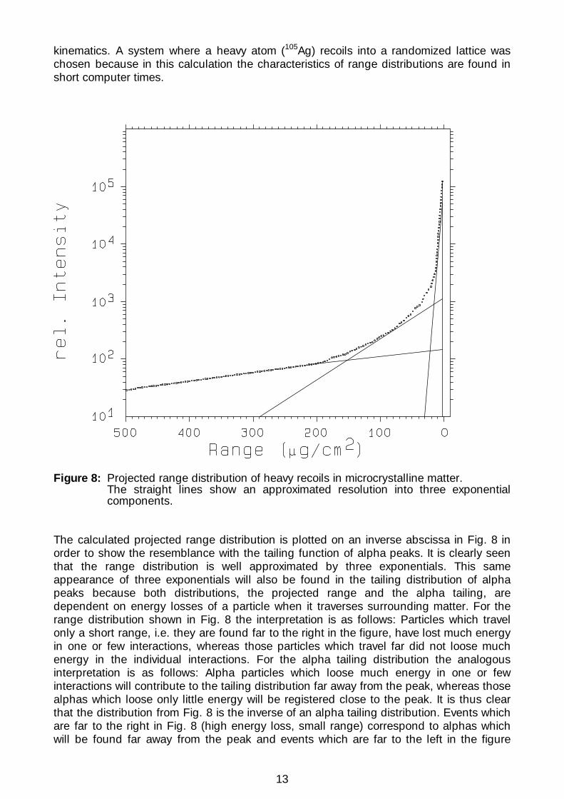
kinematics. A system where a heavy atom (105Ag) recoils into a randomized lattice was chosen because in this calculation the characteristics of range distributions are found in short computer times.

Figure 8: Projected range distribution of heavy recoils in microcrystalline matter. The straight lines show an approximated resolution into three exponential components. The calculated projected range distribution is plotted on an inverse abscissa in Fig. 8 in order to show the resemblance with the tailing function of alpha peaks. It is clearly seen that the range distribution is well approximated by three exponentials. This same appearance of three exponentials will also be found in the tailing distribution of alpha peaks because both distributions, the projected range and the alpha tailing, are dependent on energy losses of a particle when it traverses surrounding matter. For the range distribution shown in Fig. 8 the interpretation is as follows: Particles which travel only a short range, i.e. they are found far to the right in the figure, have lost much energy in one or few interactions, whereas those particles which travel far did not loose much energy in the individual interactions. For the alpha tailing distribution the analogous interpretation is as follows: Alpha particles which loose much energy in one or few interactions will contribute to the tailing distribution far away from the peak, whereas those alphas which loose only little energy will be registered close to the peak. It is thus clear that the distribution from Fig. 8 is the inverse of an alpha tailing distribution. Events which are far to the right in Fig. 8 (high energy loss, small range) correspond to alphas which will be found far away from the peak and events which are far to the left in the figure

14

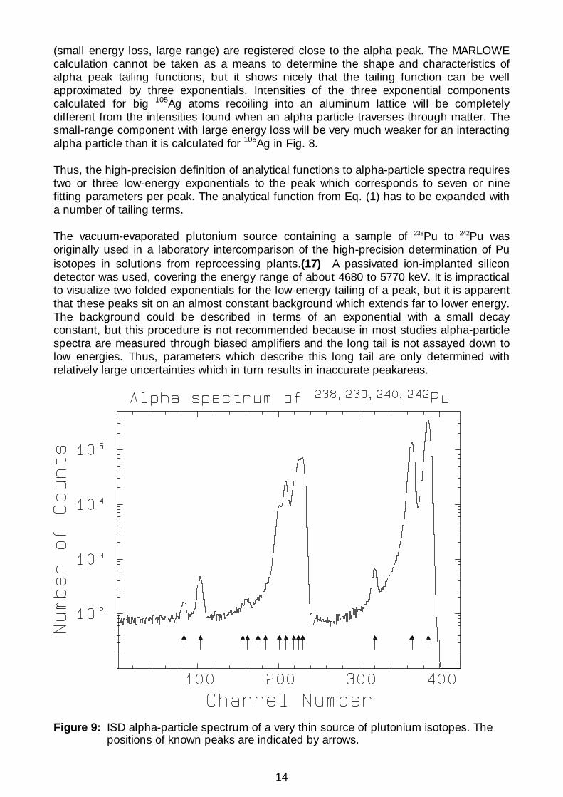
(small energy loss, large range) are registered close to the alpha peak. The MARLOWE calculation cannot be taken as a means to determine the shape and characteristics of alpha peak tailing functions, but it shows nicely that the tailing function can be well approximated by three exponentials. Intensities of the three exponential components calculated for big 105Ag atoms recoiling into an aluminum lattice will be completely different from the intensities found when an alpha particle traverses through matter. The small-range component with large energy loss will be very much weaker for an interacting alpha particle than it is calculated for 105Ag in Fig. 8. Thus, the high-precision definition of analytical functions to alpha-particle spectra requires two or three low-energy exponentials to the peak which corresponds to seven or nine fitting parameters per peak. The analytical function from Eq. (1) has to be expanded with a number of tailing terms. The vacuum-evaporated plutonium source containing a sample of 238Pu to 242Pu was originally used in a laboratory intercomparison of the high-precision determination of Pu isotopes in solutions from reprocessing plants.(17) A passivated ion-implanted silicon detector was used, covering the energy range of about 4680 to 5770 keV. It is impractical to visualize two folded exponentials for the low-energy tailing of a peak, but it is apparent that these peaks sit on an almost constant background which extends far to lower energy. The background could be described in terms of an exponential with a small decay constant, but this procedure is not recommended because in most studies alpha-particle spectra are measured through biased amplifiers and the long tail is not assayed down to low energies. Thus, parameters which describe this long tail are only determined with relatively large uncertainties which in turn results in inaccurate peakareas.

Figure 9: ISD alpha-particle spectrum of a very thin source of plutonium isotopes. The positions of known peaks are indicated by arrows.

15

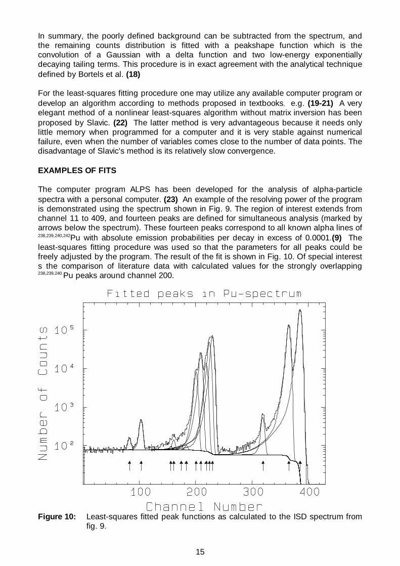
In summary, the poorly defined background can be subtracted from the spectrum, and the remaining counts distribution is fitted with a peakshape function which is the convolution of a Gaussian with a delta function and two low-energy exponentially decaying tailing terms. This procedure is in exact agreement with the analytical technique defined by Bortels et al. (18) For the least-squares fitting procedure one may utilize any available computer program or develop an algorithm according to methods proposed in textbooks, e.g. (19-21) A very elegant method of a nonlinear least-squares algorithm without matrix inversion has been proposed by Slavic. (22) The latter method is very advantageous because it needs only little memory when programmed for a computer and it is very stable against numerical failure, even when the number of variables comes close to the number of data points. The disadvantage of Slavic's method is its relatively slow convergence. EXAMPLES OF FITS The computer program ALPS has been developed for the analysis of alpha-particle spectra with a personal computer. (23) An example of the resolving power of the program is demonstrated using the spectrum shown in Fig. 9. The region of interest extends from channel 11 to 409, and fourteen peaks are defined for simultaneous analysis (marked by arrows below the spectrum). These fourteen peaks correspond to all known alpha lines of 238,239,240,242Pu with absolute emission probabilities per decay in excess of 0.0001.(9) The least-squares fitting procedure was used so that the parameters for all peaks could be freely adjusted by the program. The result of the fit is shown in Fig. 10. Of special interest s the comparison of literature data with calculated values for the strongly overlapping 238,239,240

Pu peaks around channel 200.

Figure 10: Least-squares fitted peak functions as calculated to the ISD spectrum from fig. 9.

16

In Table 1 the major peak intensities are listed as given in the literature (9,24) together with the calculated values of this work. Table 1: Comparison of calculated α-intensities with literature values __________ Nuclide α-transition Iα, literature Iα, this work % %

238Pu α0 71.6 ± 0.6 71.6 ± 1.4 α1 28.3 ±0.6 28.3 ± 0.8 α2 0.10 ± 0.03 0.11 ± 0.01

239Pu α0 73.3 ± 0.7 69.7 ± 3.5 α1 15.1 ± 0.2 19.0 ± 1.8 α2 11.5 ± 0.2 11.3 ± 0.9

240Pu α0 73.0 ± 0.3 72.4 ± 2.2 α1 27.0 ± 0.3 27.5 ± 1.1 α2 0.084 ± 0.001 0.071 ± 0.026

242Pu α0 77.5 ± 3.0 83.0 ± 7.5 α1 22.4 ± 2.0 17.0 ±4.2

Apparently the resolution of the α0 and α1 peaks of 239Pu which are both buried in the low energy flank of the dominating α0 peak of 240Pu is incomplete. However, adding the calculated intensities of the α0 and α1 peaks of 239Pu one gets an intensity of Iα0+ Iα1

= (88.7 ± 3.9) % which is in good agreement with the literature value of (88.4 ± 0.7) %, i.e., the 239Pu contribution is well resolved from the 240Pu peak. In order to test the consistency of calculated peak areas one may convert them into unnormalized atomic contents of the sample and compare the resulting atomic percentages with values obtained through two independent mass spectrometric surveys (17) of the same sample. The resulting percentages are listed in Table 2, showing an excellent agreement between this alpha spectrometric (fast) analysis and (slow) mass spectrometry. Table 2: Comparison of the isotopic contents of a plutonium reprocessing sample determined via mass- and alpha-spectrometry. ______________________________________________________ Isotope Mass spectrometer(17) This work % % ______________________________________________________ 238Pu 1.848 1.874 ± 0.050 239Pu 71.225 71.713 ± 2.909 240Pu 26.926 26.413 ± 0.883 ______________________________________________________

17

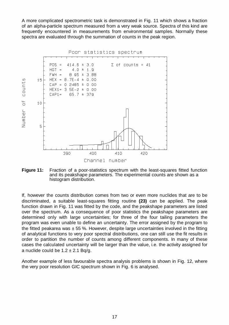
A more complicated spectrometric task is demonstrated in Fig. 11 which shows a fraction of an alpha-particle spectrum measured from a very weak source. Spectra of this kind are frequently encountered in measurements from environmental samples. Normally these spectra are evaluated through the summation of counts in the peak region.

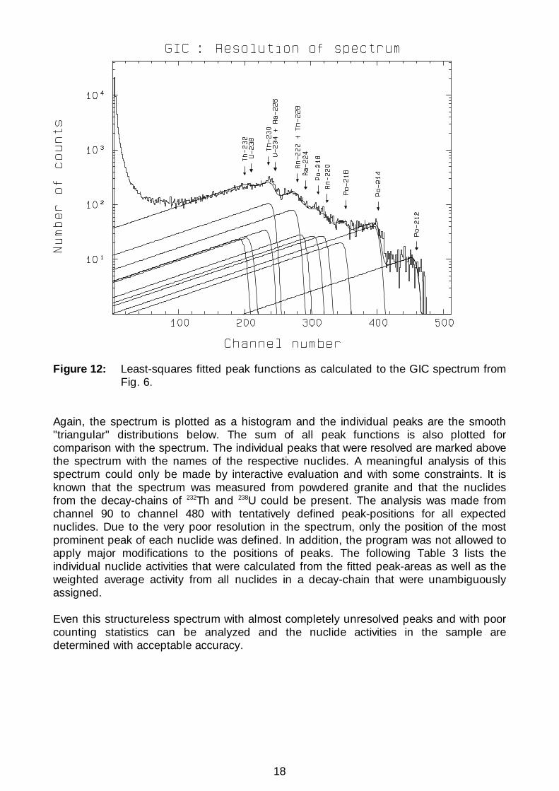
Figure 11: Fraction of a poor-statistics spectrum with the least-squares fitted function and its peakshape parameters. The experimental counts are shown as a histogram distribution. If, however the counts distribution comes from two or even more nuclides that are to be discriminated, a suitable least-squares fitting routine (23) can be applied. The peak function drawn in Fig. 11 was fitted by the code, and the peakshape parameters are listed over the spectrum. As a consequence of poor statistics the peakshape parameters are determined only with large uncertainties; for three of the four tailing parameters the program was even unable to define an uncertainty. The error assigned by the program to the fitted peakarea was ± 55 %. However, despite large uncertainties involved in the fitting of analytical functions to very poor spectral distributions, one can still use the fit results in order to partition the number of counts among different components. In many of these cases the calculated uncertainty will be larger than the value, i.e. the activity assigned for a nuclide could be 1.2 ± 2.1 Bq/g. Another example of less favourable spectra analysis problems is shown in Fig. 12, where the very poor resolution GIC spectrum shown in Fig. 6 is analysed.

18

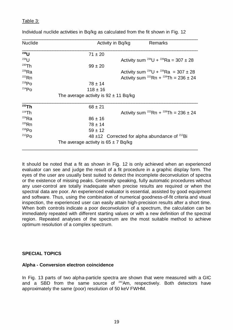
Figure 12: Least-squares fitted peak functions as calculated to the GIC spectrum from Fig. 6. Again, the spectrum is plotted as a histogram and the individual peaks are the smooth "triangular" distributions below. The sum of all peak functions is also plotted for comparison with the spectrum. The individual peaks that were resolved are marked above the spectrum with the names of the respective nuclides. A meaningful analysis of this spectrum could only be made by interactive evaluation and with some constraints. It is known that the spectrum was measured from powdered granite and that the nuclides from the decay-chains of 232Th and 238U could be present. The analysis was made from channel 90 to channel 480 with tentatively defined peak-positions for all expected nuclides. Due to the very poor resolution in the spectrum, only the position of the most prominent peak of each nuclide was defined. In addition, the program was not allowed to apply major modifications to the positions of peaks. The following Table 3 lists the individual nuclide activities that were calculated from the fitted peak-areas as well as the weighted average activity from all nuclides in a decay-chain that were unambiguously assigned. Even this structureless spectrum with almost completely unresolved peaks and with poor counting statistics can be analyzed and the nuclide activities in the sample are determined with acceptable accuracy.

19

Table 3: Individual nuclide activities in Bq/kg as calculated from the fit shown in Fig. 12 _____________________________________________________________________ Nuclide Activity in Bq/kg Remarks _____________________________________________________________________ 238U 71 ± 20 234U Activity sum 234U + 226Ra = 307 ± 28 230Th 99 ± 20 226Ra Activity sum 234U + 226Ra = 307 ± 28 222Rn Activity sum 222Rn + 228Th = 236 ± 24 218Po 78 ± 14 214Po 118 ± 16 The average activity is 92 ± 11 Bq/kg _____________________________________________________________________ 232Th 68 ± 21 228Th Activity sum 222Rn + 228Th = 236 ± 24 224Ra 86 ± 16 220Rn 78 ± 14 216Po 59 ± 12 212Po 48 ±12 Corrected for alpha abundance of 212Bi The average activity is 65 ± 7 Bq/kg _____________________________________________________________________ It should be noted that a fit as shown in Fig. 12 is only achieved when an experienced evaluator can see and judge the result of a fit procedure in a graphic display form. The eyes of the user are usually best suited to detect the incomplete deconvolution of spectra or the existence of missing peaks. Generally speaking, fully automatic procedures without any user-control are totally inadequate when precise results are required or when the spectral data are poor. An experienced evaluator is essential, assisted by good equipment and software. Thus, using the combination of numerical goodness-of-fit criteria and visual inspection, the experienced user can easily attain high-precision results after a short time. When both controls indicate a poor deconvolution of a spectrum, the calculation can be immediately repeated with different starting values or with a new definition of the spectral region. Repeated analyses of the spectrum are the most suitable method to achieve optimum resolution of a complex spectrum. SPECIAL TOPICS Alpha - Conversion electron coincidence

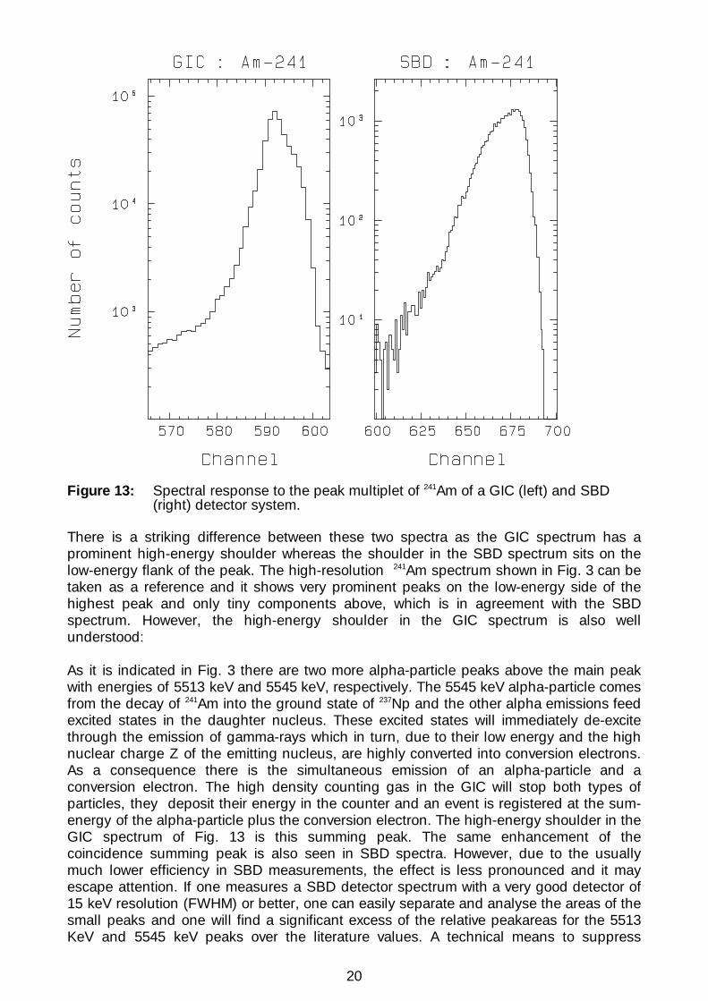
In Fig. 13 parts of two alpha-particle spectra are shown that were measured with a GIC and a SBD from the same source of 241Am, respectively. Both detectors have approximately the same (poor) resolution of 50 keV FWHM.

20

Figure 13: Spectral response to the peak multiplet of 241Am of a GIC (left) and SBD (right) detector system. There is a striking difference between these two spectra as the GIC spectrum has a prominent high-energy shoulder whereas the shoulder in the SBD spectrum sits on the low-energy flank of the peak. The high-resolution 241Am spectrum shown in Fig. 3 can be taken as a reference and it shows very prominent peaks on the low-energy side of the highest peak and only tiny components above, which is in agreement with the SBD spectrum. However, the high-energy shoulder in the GIC spectrum is also well understood: As it is indicated in Fig. 3 there are two more alpha-particle peaks above the main peak with energies of 5513 keV and 5545 keV, respectively. The 5545 keV alpha-particle comes from the decay of 241Am into the ground state of 237Np and the other alpha emissions feed excited states in the daughter nucleus. These excited states will immediately de-excite through the emission of gamma-rays which in turn, due to their low energy and the high nuclear charge Z of the emitting nucleus, are highly converted into conversion electrons. As a consequence there is the simultaneous emission of an alpha-particle and a conversion electron. The high density counting gas in the GIC will stop both types of particles, they deposit their energy in the counter and an event is registered at the sum-energy of the alpha-particle plus the conversion electron. The high-energy shoulder in the GIC spectrum of Fig. 13 is this summing peak. The same enhancement of the coincidence summing peak is also seen in SBD spectra. However, due to the usually much lower efficiency in SBD measurements, the effect is less pronounced and it may escape attention. If one measures a SBD detector spectrum with a very good detector of 15 keV resolution (FWHM) or better, one can easily separate and analyse the areas of the small peaks and one will find a significant excess of the relative peakareas for the 5513 KeV and 5545 keV peaks over the literature values. A technical means to suppress

21

coincidences with conversion electrons in SBD measurements is to apply a potential between the source and the detector, where the source is at the positive level. Geometric efficiency

When alpha-particles from radioactive decay are measured with high-density detector materials such as SBD, ISD or GIC detectors, the efficiency of the detector is defined by the solid angle subtended by the active detector surface to the source, where 4π sr are equivalent to 100 % efficiency. This direct relation between the solid angle and the efficiency is true because the heavy alpha-particle with an energy below 2.5 MeV/u is easily stopped within the high-density detector material (the projected range of decay alpha particles is less than 100 µm in Si and less than 10 cm in air at 760 Torr). The purely geometric definition of the detector efficiency is just seemingly a simplification, as can be seen from the large number of publications dealing with that subject e.g. (25-28) The solid angle can be approximately calculated to a good precision for the case of a circular detector whose planar active area is axially aligned with a circular source. Some commercially available computer codes e.g. (23) contain this calculation. If, however, the shape of the active detector surface or of the source is not circular, if the circles are not properly aligned, if the detector material is of very low density, or if the emitting source has an appreciable thickness, then the detector efficiency can hardly be calculated but it must rather be calibrated with sources of known activity for each individual geometric setup that shall later be employed for a measurement. In such a calibration measurement the geometry (shape, thickness, positioning) of source and detector must be exactly be same as in the actual measurement. If possible, one should even use calibration sources which contain the expected nuclides with about the expected activity or even better, one should spike the sample with a known amount of a non-interfering activity. Measurement of daughter nuclides

In many cases the alpha spectrum will contain peaks of a long-lived radioactive parent and also of a number of short-lived daughter nuclei in transient equilibrium. The peaks of these daughter nuclei are usually very well separated in energy from the bulk of counts in the spectrum and therefore very easily analyzed. However, one has to consider two major physical effects when the activity of a mother is evaluated via daughter nuclides: Loss of radon daughters If the source is assayed in vacuum with a SBD or ISD, then the noble gas element radon may diffuse out of the source and escape from the measurement. This effect is most prominent when the source is a thin chemical precipitate or electrodeposit, where radon losses of over 40 % have been encountered. Therefore one cannot use the nicely separated alpha peaks of polonium for a quantitative determination of radium, thorium or uranium in a sample. Efficiency corrections There are many experiments were α-decaying products are collected on a catcher or deposited on a foil after chemical sepration. These sources are then placed in front of a detector, and α-spectra are taken for activity determinations. Because of the large energy loss of α-particles in matter, one can calculate the intrinsic efficiency of a SBD from purely geometric factors (corresponding to the angle α in Fig. 14). There are disturbances to the geometrically defined detection efficiency because the charge collection from interactions near the detector edge is poor, but this effect appears to be of minor importance. Thus

22

one may define the geometric acceptance to be the average efficiency with which the detector sees the source and call it E0. For measurements of α-decays of mother and first daughter nuclides, this quantity E0 is the correct value for the detection probability. In many cases (for example, in a survey of trans-thorium reaction products) one also has to evaluate the α-lines of daughter nuclides far down the decay chain in order to obtain the formation cross-section for the mother. If the daughters have half-lives which are short compared to that of the mother, one can easily measure the decay-chain, since it is in transient equilibrium. In these cases, however, one may not take the average quantity E0 to be the detection efficiency for all daughters because when α-emitting nuclides decay, there is a 50 % probability that the α-recoil vectors are directed into the source and source holder, whereas the other 50 % are directed away from the source. The α-recoil energies of heavy α-daughter nuclei are on the order of 100 keV, which is enough for daughter nuclei to recoil out of a thin source. A fraction E0 of all decaying nuclei will be deposited on the sensitive detector face, and in the subsequent daughter-decay the alpha particle is registered with a 50 % detection efficiency. For longer decay-chains this process of recoiling to and fro will go on continuously. In order to calculate numerically the detection probabilities of daughter nuclides one must introduce four more geometric acceptance values. These values describe the probability with which a nucleus recoiling from the source (or source holder) will be deposited on the whole detector surface and vice versa.

Figure 14: Geometric model setup of SBD/source/source holder and angles defining the individual acceptances E0 through E4. The acceptances are called E1-E4 and are defined as follows: E1 = acceptance for the whole detector seeing the source (α), E2 = acceptance for the source holder seeing the whole detector (β) E3 = acceptance for the sensitive detector face seeing the source holder (δ), E4 = acceptance for the whole detector seeing the source holder (γ). The greek letters correspond to the acceptance angles shown in Fig. 14, which also shows the geometric arrangement for the determination of E1-E4. Except for the case when the source holder is deposited directly on the sensitive detector surface (E0=E1=E2=E3=E4=0.5), E0-E4 will all have different values. One can calculate these values with the usual integration method for α-efficiencies of extended sources. An explanation of the equations used to calculate the detection probabilities for daughter nuclei is given in ref. (29)

23

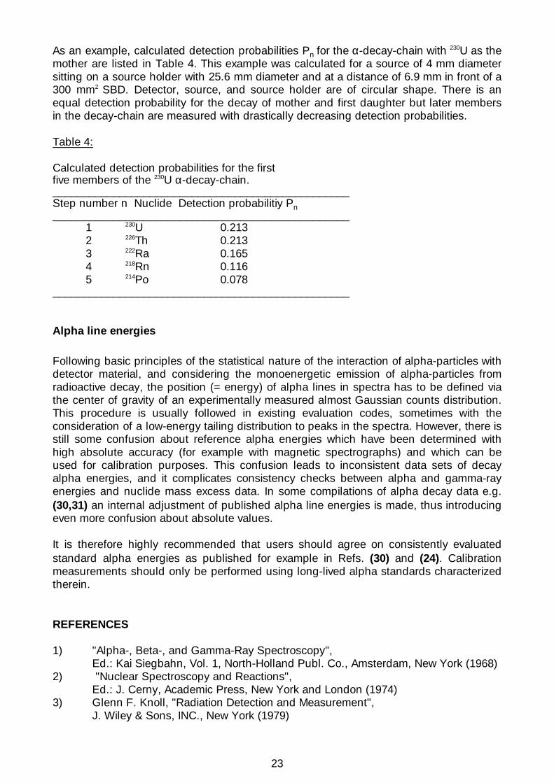
As an example, calculated detection probabilities Pn for the α-decay-chain with 230U as the mother are listed in Table 4. This example was calculated for a source of 4 mm diameter sitting on a source holder with 25.6 mm diameter and at a distance of 6.9 mm in front of a 300 mm2 SBD. Detector, source, and source holder are of circular shape. There is an equal detection probability for the decay of mother and first daughter but later members in the decay-chain are measured with drastically decreasing detection probabilities. Table 4: Calculated detection probabilities for the first five members of the 230U α-decay-chain. _________________________________________________ Step number n Nuclide Detection probabilitiy Pn _________________________________________________ 1 230U 0.213 2 226Th 0.213 3 222Ra 0.165 4 218Rn 0.116 5 214Po 0.078 _________________________________________________ Alpha line energies

Following basic principles of the statistical nature of the interaction of alpha-particles with detector material, and considering the monoenergetic emission of alpha-particles from radioactive decay, the position (= energy) of alpha lines in spectra has to be defined via the center of gravity of an experimentally measured almost Gaussian counts distribution. This procedure is usually followed in existing evaluation codes, sometimes with the consideration of a low-energy tailing distribution to peaks in the spectra. However, there is still some confusion about reference alpha energies which have been determined with high absolute accuracy (for example with magnetic spectrographs) and which can be used for calibration purposes. This confusion leads to inconsistent data sets of decay alpha energies, and it complicates consistency checks between alpha and gamma-ray energies and nuclide mass excess data. In some compilations of alpha decay data e.g. (30,31) an internal adjustment of published alpha line energies is made, thus introducing even more confusion about absolute values. It is therefore highly recommended that users should agree on consistently evaluated standard alpha energies as published for example in Refs. (30) and (24). Calibration measurements should only be performed using long-lived alpha standards characterized therein. REFERENCES 1) "Alpha-, Beta-, and Gamma-Ray Spectroscopy", Ed.: Kai Siegbahn, Vol. 1, North-Holland Publ. Co., Amsterdam, New York (1968) 2) "Nuclear Spectroscopy and Reactions", Ed.: J. Cerny, Academic Press, New York and London (1974) 3) Glenn F. Knoll, "Radiation Detection and Measurement", J. Wiley & Sons, INC., New York (1979)

24

4) "Detectors in Nuclear Science", Ed.: A. Bromley, Nucl. Instr. Meth. 162 (1979) Nos. 1-3 5) Nuclear Instruments and Methods in Physics Research Sections A: Spectrometers, Detectors and Associated Equipment. 226 (1984) p.1-218 6) M. Ivanovich and R. M. Warchal, Report AERE-R 10044, AEAE, Harwell (1981) 7) After: ORTEC Application Note AN34 (1976), Experiment 4. 8) "Nuclear spectroscopy at room temperature", Technical Note, Enertec/Schlumberger (1983) 9) W. Westmeier and A. Merklin, Physik Daten/Physics Data 29-1 (1985) 1-88 Fachinformationszentrum EPM GmbH, Karlsruhe, FRG 10) GIC spectra, courtesy of Prof. Dr. B. Sansoni from KfA Jülich GmbH. 11) W. Westmeier, Nucl. Instr. Meth. A242 (1986) 437 12) W. Wätzig and W. Westmeier, Nucl. Instr. Meth. 153 (1978) 517 13) A. L'Hoir, Nucl. Instr. Meth. 223 (1984) 336 14) W. Westmeier, Thesis, Philipps-Universität Marburg (1981) unpublished 15) W. Westmeier, Int. J. Appl. Radiat. Isot. 35-4 (1983) 236 16) M.T. Robinson and I.M. Torrens, Phys. Rev. B9-12 (1974) 5008 17) G. Bortels et al., Report No. KfK2862/EUR6402e, Part III, Kernforschungszentrum Karlsruhe (1979) 18) G. Bortels and P. Collaers, Appl. Radiat. Isot. 38-10 (1987) 831 19) William H. Press et al., "Numerical Recipes", Cambridge University Press, Cambridge, New York, Melbourne (1986) 20) S. Brandt, "Datenanalyse", 3. Auflage, Bibliographisches Institut, Mannheim (1988)

25

21) J. Dreszer, "Mathematik Handbuch", Verlag Harri Deutsch, Zürich-Frankfurt/Main-Thun (1975) 22) Ilfan A. Slavic, Nucl. Instr. Meth. 134 (1976) 285 23) Dr. Westmeier GmbH, "ALPS, a program for the high-precision analysis of alpha-particle spectra", commercial product 24) "Proposed Recommended List of Heavy Element Radionuclide Decay Data", IAEA Report INDC(NDS)-149/NE, ed. by A. Lorenz, IAEA, Wien (1983) 25) C. L. Lindeken and D. N. Montan, Health Physics 13 (1967) 405 26) M. P. Ruffle, Nucl. Instr. Meth. 52 (1967) 354 27) R. P. Gardner and K. Vergese, Nucl. Instr. Meth. 93 (1971) 163 28) U. Prösch et al., Isotopenpraxis 10 (1979) 297 29) W. Westmeier, Nucl. Instr. Meth. 163 (1979) 593 30) A. Rytz, Atomic Data and Nuclear Data Tables 47 (1991) 205 31) Nuclear Data Sheets, Ed.: M. J. Martin and J. K. Tuli, Academic Press INC., New York