Embed Size (px)
Citation preview

ISSN 0015-4628, Fluid Dynamics, 2021, Vol. 56, No. 4, pp. 513–538. © The Author(s), 2021. This article is an open access publication.Russian Text © The Author(s), 2021, published in Izvestiya RAN. Mekhanika Zhidkosti i Gaza, 2021, Vol. 56, No. 4, pp. 73–99.
Prandtl’s Secondary Flows of the Second Kind.Problems of Description, Prediction, and Simulation
N. V. Nikitina,*, N. V. Popelenskayaa,**, and A. Strohb,***a Institute of Mechanics, Moscow State University, Michurinskii pr. 1, Moscow, 119192 Russia
b Institute of Fluid Mechanics, Karlsruhe Institute of Technology, Karlsruhe, Germany*e-mail: [email protected]
**e-mail: [email protected]***e-mail: [email protected]
Received March 23, 2021; revised March 25, 2021; accepted March 25, 2021
Abstract—The occurrence of turbulent pulsations in straight pipes of noncircular cross-section leadsto the situation, when the average velocity field includes not only the longitudinal component but alsotransverse components that form a secondary f low. This hydrodynamic phenomenon discovered atthe twenties of the last century (J. Nikuradse, L. Prandtl) has been the object of active research to thepresent day. The intensity of the turbulent secondary f lows is not high; usually, it is not greater than2–3% of the characteristic f low velocity. Nevertheless, their contribution to the processes of transversetransfer of momentum and heat is comparable to that of turbulent pulsations. In this paper, a reviewof experimental, theoretical, and numerical studies of secondary f lows in straight pipes and channelsis given. Emphasis is placed on the issues of revealing the physical mechanisms of secondary f low for-mation and developing the models of the apriori assessment of their forms. The specific features of thesecondary f low development in open channels and channels with inhomogeneously rough walls aretouched upon. The approaches of semiempirical simulation of turbulent f lows in the presence of sec-ondary f lows are discussed.
Keywords: turbulent f lows in straight pipes, secondary f lows, Navier–Stokes equations, direct numer-ical simulation, rough walls, RANS modeling
DOI: 10.1134/S0015462821040091
One of the interesting and practically important manifestations of turbulence is the capability to inducethe so-named secondary f lows, that is, organized f luid motions in the plane perpendicular to the mainstream direction. The most known in this respect are f lows in straight pipes of noncircular cross-section.Fairly far from the entry laminar f lows in these pipes are one-dimensional, that is, at any point the f luidvelocity is directed along the pipe. Contrariwise, in turbulent regimes the average velocity field containsnonzero transverse components. The first experimental evidence of the generation of turbulent secondaryflows was obtained by Nikuradse in pipes with rectangular and triangular cross-sections [1]. He found thatthe isotachs (contours of the mean longitudinal velocity in the cross-sectional plane) have unusual con-vexities directed toward the corners (Fig. 1). Prandtl supposed that the characteristic distortions of the iso-tachs are caused by secondary f lows induced by turbulent pulsations. The f luid f lows along the bisectortoward the corner and spreads on both sides along the walls. Thus, the f luid particles with a greatermomentum are transferred from the f low core to the walls, into the corner region, which gives rise to ananomalous velocity increase in this region of the pipe [2–4] (Fig. 2). Prandtl’s supposition on the occur-rence of secondary f lows in straight noncircular pipes was confirmed in [5] by mean velocity measure-ments and turbulent f low visualization in pipes with different cross-sections. In those times the secondaryflow intensity could not be reliably measured. The first direct measurements of the secondary f lows inrectangular pipes were carried out only 30 years later [6]. Secondary f lows in straight pipes occur only inturbulent f lows. Prandtl [7, 8] proposed to call these f lows the secondary f lows of the second kind, as dis-tinct from the secondary f lows of the first kind occurring within curved f lows under the action of centrif-ugal effects in both turbulent and laminar f lows. The intensity of the secondary f lows of the first kind canbe as high as tens of percents of the main stream velocity. The characteristic velocities of the secondaryflows of the second kind are considerably lower. In pipes they are usually not greater than 2–3%. None-
513
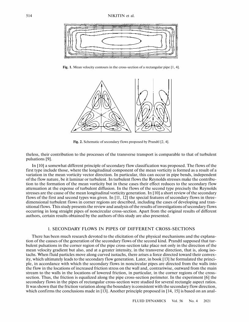
514 NIKITIN et al.
Fig. 1. Mean velocity contours in the cross-section of a rectangular pipe [1, 4].
Fig. 2. Schematic of secondary f lows proposed by Prandtl [2, 4].
theless, their contribution to the processes of the transverse transport is comparable to that of turbulentpulsations [9].
In [10] a somewhat different principle of secondary f low classification was proposed. The f lows of thefirst type include those, where the longitudinal component of the mean vorticity is formed as a result of avariation in the mean vorticity vector direction. In particular, this can occur in pipe bends, independentof the f low nature, be it laminar or turbulent. In turbulent f lows the Reynolds stresses make the contribu-tion to the formation of the mean vorticity but in these cases their effect reduces to the secondary f lowattenuation at the expense of turbulent diffusion. In the f lows of the second type precisely the Reynoldsstresses are the cause of the mean longitudinal vorticity generation. In [10] a short review of the secondaryflows of the first and second types was given. In [11, 12] the special features of secondary f lows in three-dimensional turbulent f lows in corner regions are described, including the cases of developing and tran-sitional f lows. This study presents the review and analysis of the results of investigations of secondary f lowsoccurring in long straight pipes of noncircular cross-section. Apart from the original results of differentauthors, certain results obtained by the authors of this study are also presented.
1. SECONDARY FLOWS IN PIPES OF DIFFERENT CROSS-SECTIONS
There has been much research devoted to the elicitation of the physical mechanisms and the explana-tion of the causes of the generation of the secondary f lows of the second kind. Prandtl supposed that tur-bulent pulsations in the corner region of the pipe cross-section take place not only in the direction of themean velocity gradient but also, and at a greater intensity, in the transverse direction, that is, along iso-tachs. When f luid particles move along curved isotachs, there arises a force directed toward their convex-ity, which ultimately leads to the secondary f low generation. Later, in book [13] he formulated the princi-ple, in accordance with which the secondary f lows in noncircular pipes are directed from the walls intothe f low in the locations of increased friction stress on the wall and, contrariwise, outward from the mainstream to the walls in the locations of lowered friction, in particular, in the corner regions of the cross-section. Thus, the friction is equalized along the pipe cross-section perimeter. In the experiment [6] thesecondary f lows in the pipes of rectangular cross-section were studied for several rectangle aspect ratios.It was shown that the friction variation along the boundary is consistent with the secondary f low direction,which confirms the conclusions made in [13]. Another principle proposed in [14, 15] is based on an anal-
FLUID DYNAMICS Vol. 56 No. 4 2021
PRANDTL’S SECONDARY FLOWS OF THE SECOND KIND 515
ysis of the terms of the balance equation for the kinetic energy of turbulence. If at certain location of theflow the kinetic energy production is considerably greater than viscous dissipation, then there arises a sec-ondary f low transferring the f luid particles with a greater kinetic energy from this region toward theregions, where the energy production is inferior than dissipation.
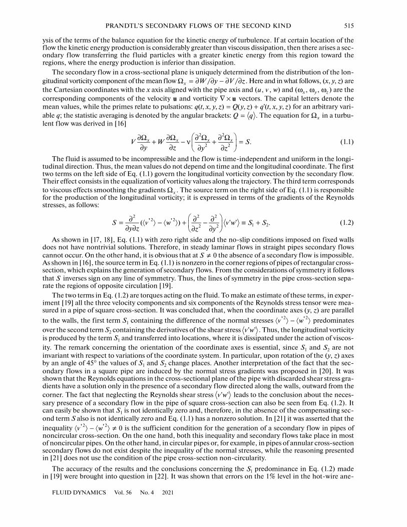
The secondary f low in a cross-sectional plane is uniquely determined from the distribution of the lon-gitudinal vorticity component of the mean flow . Here and in what follows, (x, y, z) arethe Cartesian coordinates with the x axis aligned with the pipe axis and ( , , w) and ( , , ) are thecorresponding components of the velocity and vorticity vectors. The capital letters denote themean values, while the primes relate to pulsations: for an arbitrary vari-able q; the statistic averaging is denoted by the angular brackets: . The equation for in a turbu-lent f low was derived in [16]
(1.1)
The fluid is assumed to be incompressible and the f low is time-independent and uniform in the longi-tudinal direction. Thus, the mean values do not depend on time and the longitudinal coordinate. The firsttwo terms on the left side of Eq. (1.1) govern the longitudinal vorticity convection by the secondary f low.Their effect consists in the equalization of vorticity values along the trajectory. The third term correspondsto viscous effects smoothing the gradients . The source term on the right side of Eq. (1.1) is responsiblefor the production of the longitudinal vorticity; it is expressed in terms of the gradients of the Reynoldsstresses, as follows:
(1.2)
As shown in [17, 18], Eq. (1.1) with zero right side and the no-slip conditions imposed on fixed wallsdoes not have nontrivial solutions. Therefore, in steady laminar f lows in straight pipes secondary f lowscannot occur. On the other hand, it is obvious that at the absence of a secondary f low is impossible.As shown in [16], the source term in Eq. (1.1) is nonzero in the corner regions of pipes of rectangular cross-section, which explains the generation of secondary f lows. From the considerations of symmetry it followsthat inverses sign on any line of symmetry. Thus, the lines of symmetry in the pipe cross-section sepa-rate the regions of opposite circulation [19].
The two terms in Eq. (1.2) are torques acting on the f luid. To make an estimate of these terms, in exper-iment [19] all the three velocity components and six components of the Reynolds stress tensor were mea-sured in a pipe of square cross-section. It was concluded that, when the coordinate axes (y, z) are parallelto the walls, the first term S1 containing the difference of the normal stresses predominatesover the second term S2 containing the derivatives of the shear stress . Thus, the longitudinal vorticityis produced by the term S1 and transferred into locations, where it is dissipated under the action of viscos-ity. The remark concerning the orientation of the coordinate axes is essential, since S1 and are notinvariant with respect to variations of the coordinate system. In particular, upon rotation of the (y, z) axesby an angle of 45° the values of S1 and S2 change places. Another interpretation of the fact that the sec-ondary f lows in a square pipe are induced by the normal stress gradients was proposed in [20]. It wasshown that the Reynolds equations in the cross-sectional plane of the pipe with discarded shear stress gra-dients have a solution only in the presence of a secondary f low directed along the walls, outward from thecorner. The fact that neglecting the Reynolds shear stress leads to the conclusion about the neces-sary presence of a secondary f low in the pipe of square cross-section can also be seen from Eq. (1.2). Itcan easily be shown that S1 is not identically zero and, therefore, in the absence of the compensating sec-ond term S also is not identically zero and Eq. (1.1) has a nonzero solution. In [21] it was asserted that theinequality is the sufficient condition for the generation of a secondary f low in pipes ofnoncircular cross-section. On the one hand, both this inequality and secondary f lows take place in mostof noncircular pipes. On the other hand, in circular pipes or, for example, in pipes of annular cross-sectionsecondary f lows do not exist despite the inequality of the normal stresses, while the reasoning presentedin [21] does not use the condition of the pipe cross-section non-circularity.
The accuracy of the results and the conclusions concerning the predominance in Eq. (1.2) madein [19] were brought into question in [22]. It was shown that errors on the 1% level in the hot-wire ane-
Ω = ∂ ∂ − ∂ ∂/ /x W y V zu v ωx ωy ωz
u ∇ × u, , , = , + , , ,( ) ( ) '( )q t x y z Q y z q t x y z
=Q q Ωx
∂Ω ∂Ω ∂ Ω ∂ Ω+ − ν + = ∂ ∂ ∂ ∂
2 2
2 2 .x x x xV W Sy z y z
Ωx
∂ ∂ ∂= − + − ≡ + ∂ ∂ ∂ ∂
2 2 22 2
1 22 2' '( ) ' ' .S w w S S
y z z yv v
≠ 0S
S
− v2 2' 'w
v' 'w
2S
v' 'w
− ≠v2 2' ' 0w
1S
FLUID DYNAMICS Vol. 56 No. 4 2021
516 NIKITIN et al.
mometer signal in the measurement system used can lead to 100% errors in evaluating the shear stresses. More accurate measurements [23] showed that the Reynolds stress gradients generating the
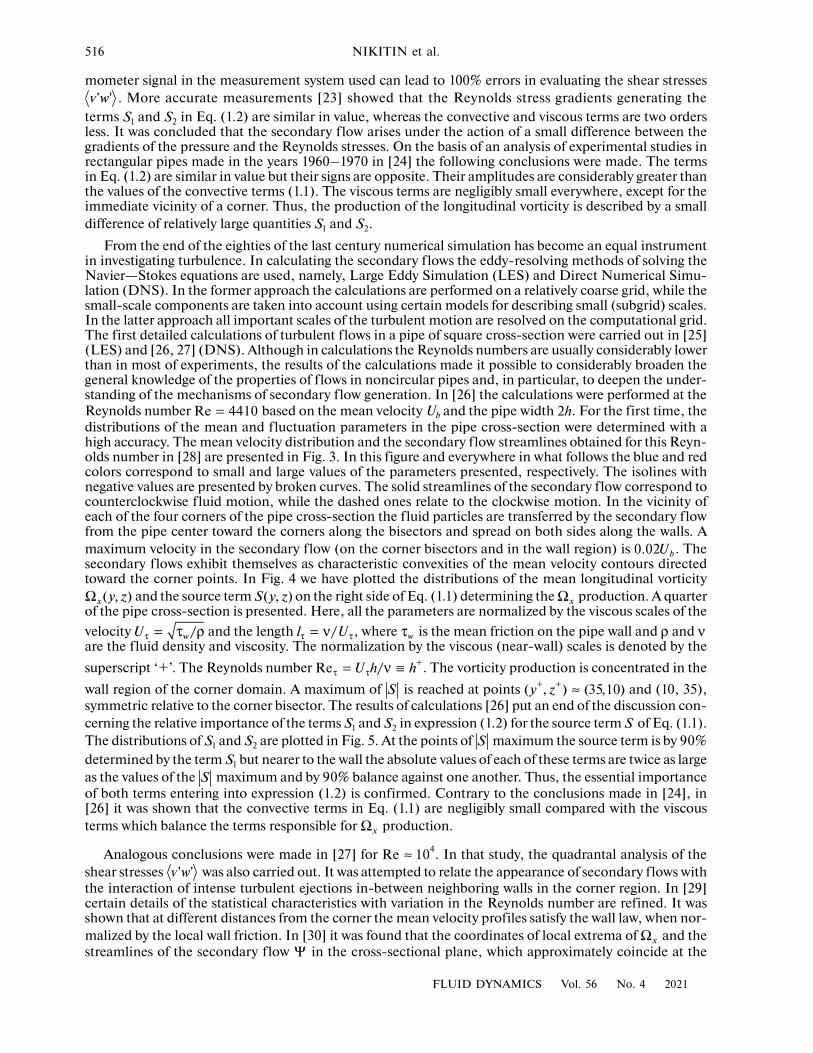
terms and in Eq. (1.2) are similar in value, whereas the convective and viscous terms are two ordersless. It was concluded that the secondary f low arises under the action of a small difference between thegradients of the pressure and the Reynolds stresses. On the basis of an analysis of experimental studies inrectangular pipes made in the years 1960–1970 in [24] the following conclusions were made. The termsin Eq. (1.2) are similar in value but their signs are opposite. Their amplitudes are considerably greater thanthe values of the convective terms (1.1). The viscous terms are negligibly small everywhere, except for theimmediate vicinity of a corner. Thus, the production of the longitudinal vorticity is described by a smalldifference of relatively large quantities and .
From the end of the eighties of the last century numerical simulation has become an equal instrumentin investigating turbulence. In calculating the secondary f lows the eddy-resolving methods of solving theNavier—Stokes equations are used, namely, Large Eddy Simulation (LES) and Direct Numerical Simu-lation (DNS). In the former approach the calculations are performed on a relatively coarse grid, while thesmall-scale components are taken into account using certain models for describing small (subgrid) scales.In the latter approach all important scales of the turbulent motion are resolved on the computational grid.The first detailed calculations of turbulent f lows in a pipe of square cross-section were carried out in [25](LES) and [26, 27] (DNS). Although in calculations the Reynolds numbers are usually considerably lowerthan in most of experiments, the results of the calculations made it possible to considerably broaden thegeneral knowledge of the properties of f lows in noncircular pipes and, in particular, to deepen the under-standing of the mechanisms of secondary f low generation. In [26] the calculations were performed at theReynolds number based on the mean velocity Ub and the pipe width . For the first time, thedistributions of the mean and fluctuation parameters in the pipe cross-section were determined with ahigh accuracy. The mean velocity distribution and the secondary f low streamlines obtained for this Reyn-olds number in [28] are presented in Fig. 3. In this figure and everywhere in what follows the blue and redcolors correspond to small and large values of the parameters presented, respectively. The isolines withnegative values are presented by broken curves. The solid streamlines of the secondary f low correspond tocounterclockwise f luid motion, while the dashed ones relate to the clockwise motion. In the vicinity ofeach of the four corners of the pipe cross-section the f luid particles are transferred by the secondary f lowfrom the pipe center toward the corners along the bisectors and spread on both sides along the walls. Amaximum velocity in the secondary f low (on the corner bisectors and in the wall region) is . Thesecondary f lows exhibit themselves as characteristic convexities of the mean velocity contours directedtoward the corner points. In Fig. 4 we have plotted the distributions of the mean longitudinal vorticity
and the source term on the right side of Eq. (1.1) determining the production. A quarterof the pipe cross-section is presented. Here, all the parameters are normalized by the viscous scales of thevelocity and the length , where is the mean friction on the pipe wall and and are the f luid density and viscosity. The normalization by the viscous (near-wall) scales is denoted by thesuperscript ‘+’. The Reynolds number . The vorticity production is concentrated in thewall region of the corner domain. A maximum of is reached at points and (10, 35),symmetric relative to the corner bisector. The results of calculations [26] put an end of the discussion con-cerning the relative importance of the terms and in expression (1.2) for the source term of Eq. (1.1).The distributions of and are plotted in Fig. 5. At the points of maximum the source term is by 90%determined by the term but nearer to the wall the absolute values of each of these terms are twice as largeas the values of the maximum and by 90% balance against one another. Thus, the essential importanceof both terms entering into expression (1.2) is confirmed. Contrary to the conclusions made in [24], in[26] it was shown that the convective terms in Eq. (1.1) are negligibly small compared with the viscousterms which balance the terms responsible for production.
Analogous conclusions were made in [27] for . In that study, the quadrantal analysis of theshear stresses was also carried out. It was attempted to relate the appearance of secondary f lows withthe interaction of intense turbulent ejections in-between neighboring walls in the corner region. In [29]certain details of the statistical characteristics with variation in the Reynolds number are refined. It wasshown that at different distances from the corner the mean velocity profiles satisfy the wall law, when nor-malized by the local wall friction. In [30] it was found that the coordinates of local extrema of and thestreamlines of the secondary f low in the cross-sectional plane, which approximately coincide at the
v' 'w1S 2S
1S 2S
=Re 4410 2h
.0 02 bU
Ω ,( )x y z ,( )S y z Ωx
τ = τ ρ/wU τ τ= ν/l U τw ρ ν
+τ τ= ν ≡Re /U h h
S + +, ≈ ,( ) (35 10)y z
1S 2S S1S 2S S
1SS
Ωx
≈ 4Re 10v' 'w
ΩxΨ
FLUID DYNAMICS Vol. 56 No. 4 2021

PRANDTL’S SECONDARY FLOWS OF THE SECOND KIND 517
Fig. 3. Mean velocity distribution U/Ub (a) and secondary f low streamlines (stream function contours, ) (b) in the cross-section of a square pipe at [26, 28].
�0.5
�0.5 0.5 1.00�0.5 0.5 1.00 �1.0
0.5
1.0
0
�0.5
�1.0
0.5
1.0(a) (b)z/h z/h
y/h y/h
0
���������
���������
���
���
���
���������
������������
���
���
���������
���������
���������
���
���
���
��
��
��
Ψ = ± ./ 0 0004bh U n = −1 6n =Re 4410
Fig. 4. Distributions of the mean longitudinal vorticity , (a) and the source term in Eq. (1.1)
, (b) in the cross-section of a square pipe at ( ) [26, 28].
150z+
100
50
0
150z+
y+y+
100
50
050 100 150 50 100 150
(a) (b)
+Ω = ± .0 01x n = −1 6n+ = ± .0 0001S n = −1 7n =Re 4410 τ =Re 150
lowest Reynolds numbers , diverge at greater Re values. In this case, the coordinates of localextrema of no longer vary with increase in Re, when expressed in viscous units. On the contrary, thecoordinates of extrema of remain constant on the global scale. A certain statistical relationship betweenthe secondary f low and turbulent near-wall structures, such as streaky structures occurring in the wallregion of a turbulent boundary layer, can be observable. The streaky structures that are closest to the cor-ner have predominantly an elevated velocity and are formed at a distance of 50 viscous lengths. In thiscase, the sign of the quasilongitudinal vortices in the wall region predominantly coincides with the signof . In [31], where LES calculations were performed for three Reynolds numbers, ( ), it was concluded that, when normalized by the viscous scales, the values and distri-butions of the terms corresponding to viscous diffusion and the longitudinal vorticity production inEq. (1.1) do not change with variation in . DNS calculations were carried out in [32] up to ( ). Emphasis was placed on the refinement of the distributions of the mean velocity compo-nents and the pulsation intensities. The calculations up to even greater values were performedin [33]. It was shown that outside the corner region the secondary f lows can be at a good accuracy approx-imated by the eigenfunctions of the Laplace operator. It was concluded that at high Reynolds numbers theeffect of the secondary f lows on the integral properties of the f low is only slight.
∼Re 2000Ωx
Ψ
Ωx τ = , ,Re 190 300 550≈ −Re 6000 20000
Re τ =Re 600≈Re 21400
≈Re 40000
FLUID DYNAMICS Vol. 56 No. 4 2021
518 NIKITIN et al.
Fig. 5. Distributions of the quantities and (1.2) in the cross-section of a square pipe at ( ) [26, 28];
, (a) and , (b).
150z+
100
50
0
150z+
y+y+
100
50
050 100 150 50 100 150
(a) (b)
1S 2S =Re 4410 τ =Re 150+ = ± .1 0 0002S n = −1 7n + = ± .2 0 0002S n = −1 6n
Fig. 6. Distribution of the mean velocity U/Ub (a) and secondary f low streamlines (stream function contours, ) (b) in the cross-section of a rectangular pipe with the aspect ratio 4:1 at [34].
�0.5
�3 �2 �1 0�1.0
0.5
1.0
0
�1.0
�0.5
�4
0.5
1.0(a) (b)z/h z/h
y/h�3 �2 �1 0�4
y/h
0
���������
������������������
���������
���������
���������
���������
���������
��Ψ = ± ./ 0 0005bh U n = −1 8n =Re 4410
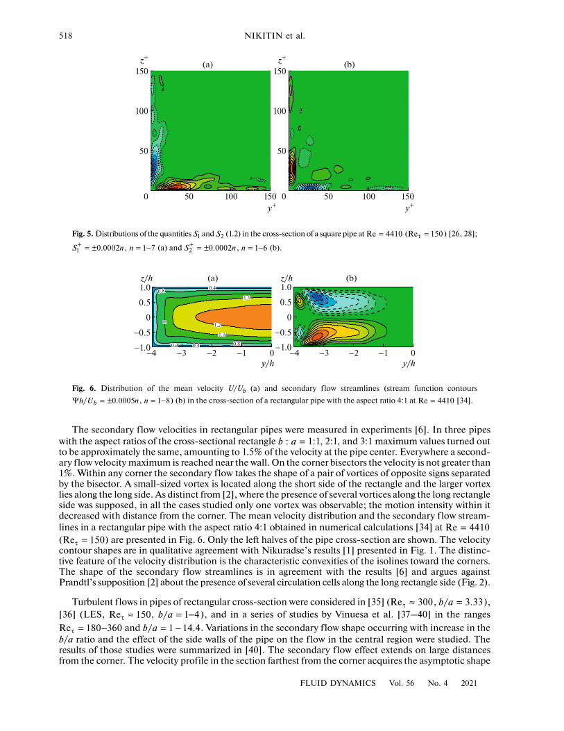
The secondary f low velocities in rectangular pipes were measured in experiments [6]. In three pipeswith the aspect ratios of the cross-sectional rectangle 1:1, 2:1, and 3:1 maximum values turned outto be approximately the same, amounting to 1.5% of the velocity at the pipe center. Everywhere a second-ary f low velocity maximum is reached near the wall. On the corner bisectors the velocity is not greater than1%. Within any corner the secondary f low takes the shape of a pair of vortices of opposite signs separatedby the bisector. A small-sized vortex is located along the short side of the rectangle and the larger vortexlies along the long side. As distinct from [2], where the presence of several vortices along the long rectangleside was supposed, in all the cases studied only one vortex was observable; the motion intensity within itdecreased with distance from the corner. The mean velocity distribution and the secondary f low stream-lines in a rectangular pipe with the aspect ratio 4:1 obtained in numerical calculations [34] at ( ) are presented in Fig. 6. Only the left halves of the pipe cross-section are shown. The velocitycontour shapes are in qualitative agreement with Nikuradse’s results [1] presented in Fig. 1. The distinc-tive feature of the velocity distribution is the characteristic convexities of the isolines toward the corners.The shape of the secondary f low streamlines is in agreement with the results [6] and argues againstPrandtl’s supposition [2] about the presence of several circulation cells along the long rectangle side (Fig. 2).
Turbulent f lows in pipes of rectangular cross-section were considered in [35] ( , ),[36] (LES, , ), and in а series of studies by Vinuesa et al. [37–40] in the ranges
and . Variations in the secondary f low shape occurring with increase in theb/a ratio and the effect of the side walls of the pipe on the f low in the central region were studied. Theresults of those studies were summarized in [40]. The secondary f low effect extends on large distancesfrom the corner. The velocity profile in the section farthest from the corner acquires the asymptotic shape
: =b a
=Re 4410τ =Re 150
τ ≈Re 300 = ./ 3 33b aτ ≈Re 150 = −/ 1 4b a
τ = −Re 180 360 = − ./ 1 14 4b a
FLUID DYNAMICS Vol. 56 No. 4 2021
PRANDTL’S SECONDARY FLOWS OF THE SECOND KIND 519
only for . For the purpose of possible attenuation of the secondary f low Vidal et al. [41–43] inves-tigated f low in rectangular tubes with rounded corners. Contrary to the expectations, the rounding of thecorners did not lead to the secondary f low attenuation and in certain cases even favored its enhancement.The vortices are formed near the junctions between the roundednesses and straight regions. In the casesin which a straight lateral wall in a rectangular pipe was replaced by a semicircular wall, only one vortexeach is formed near the junction between the semicircle and the long rectilinear walls rather than conven-tional four vortices (a vortex pair each near each angle).
In [9] turbulent f low in pipes of elliptical cross-section were calculated. The calculations were carriedout in the Cartesian coordinate system. The no-slip boundary conditions on the curvilinear boundarieswere satisfied using the method of virtual boundaries [44]. The f lows in the pipes with ellipse semiaxisratios and 1/2 were studied for . It was found that in both cases the secondary f lowstake the form of two vortex pairs of opposite sign. The f luid f lows from the pipe center toward the wallsalong the large semiaxes, spreads along the walls to both sides, and returns from the walls to the pipe centeralong the short semiaxes. In the f low core the greatest secondary f low velocity is less than 1% of the meanvelocity, while near the walls it amounts to 1 and 1.4% in the wide and narrow pipes, respectively. Despitethe so small intensity, the secondary f lows have a considerable effect on the mean flow velocity distribu-tion in the pipe cross-section, which is comparable with the effect of turbulent stresses. The effects of thesecondary f lows and turbulent stresses are opposite: the former tend to extend the velocity contours alongthe large ellipse semiaxes, whereas the turbulent stresses constrict them toward the pipe center. To moreaccurately reproduce the f low details in the wall region in [45, 46] the calculations of f lows in ellipticalpipes were carried out. In those studies the Navier—Stokes equations were solved in the elliptical cylin-drical coordinate system in which the pipe wall coincides with a coordinate surface. The method of solvingthe Navier—Stokes equations in an arbitrary curvilinear coordinate system [47] was used. The inferencesmade in [9] were confirmed and refined and the terms of Eq. (1.1) for the longitudinal vorticity wereassessed. The source term on the right side of Eq. (1.1) has noticeable nonzero values only in a narrowwall layer, where it can be represented similarly to Eq. (1.2) in the form of the sum of two terms, of whichthe first, , is the second mixed derivative of the difference between the normal Reynolds stresses, whilethe second, , is the difference of the second derivatives of the Reynolds shear stress. Elementary esti-mates show that and act as the longitudinal vorticity source and sink, respectively. The and distributions in the pipe cross-section turn out to be surprisingly similar in shape, amounting to about30% of .
In the pipes of circular cross-section secondary f lows do not occur due to the central symmetry of theflow. Obviously that in the pipes of annular cross-section secondary f lows do not arise for the same rea-son. Secondary f lows in the pipes with eccentric annular cross-section were studied experimentally in [48,49]. According to measurements [48], the secondary f low takes the shape of pairwise, oppositely directedvortices, placed symmetrically relative to the line of symmetry in the cross-sectional plane. Circulationcells are mostly pressed against the inner cylinder. The f luid moves from the narrow gap toward the widegap along the inner cylinder and returns backward, approximately midway between the cylinders. In thewidest part of the gap the secondary f low velocity is directed from the inner to the outer cylinder. In [49]the secondary f low direction was opposite. Moreover, in the narrow part of the gap one more pair of vor-tices of smaller intensity was noticed. We note that the plausibility of both results is not high, which wasadmitted by their authors themselves. Moreover, the measurements in the two cited experiments wereconducted for considerably differing geometric parameters and Reynolds numbers. In [50, 51] direct cal-culations of turbulent f low in eccentric annular pipes were carried out at two Reynolds numbers
and 8000. The algorithm [47] was applied in the bicylindrical coordinate system, in which bothpipe walls are coordinate surfaces. The secondary f low pattern thus obtained resembles the results of [48]:the f luid particles move along the inner cylinder from the narrow to the wide gap and return backward inthe mid-cross-section. Nearer to the outer cylinder, from the side of the wide gap there is a less intensecirculation cell with opposite rotation direction. Topologically equivalent secondary f low pattern with twovortices of opposite sign in each half of the cross-section was obtained numerically in [52]. However, asdistinct from [50, 51], the less intense vortex is located in the narrow rather than in the wide part of thegap. These differences in the secondary f low shapes can be attributed to a considerable difference in thegeometries of the pipes considered in [50, 51] and [52].
Secondary f lows along external corners are studied in less detail. We can note only the experimentsperformed in the Melbourne University [53–55] and numerical calculations [56, 57]. In the experimentsa f low along a ridge formed by two f lat plates joined at right angle was studied. In the calculations f low inin a gap between two pipes of square cross-section nested within each other was considered; the pipe had
>/ 10b a
=/ 2/3b a =Re 6000
S
1S2S
1S 2S 1S − 2S2S
1S
=Re 4000
FLUID DYNAMICS Vol. 56 No. 4 2021
520 NIKITIN et al.
Fig. 7. Distribution of the mean velocity U/Ub (a) and secondary f low streamlines (stream function contours, ) (b) in the cross-section of a pipe with an external angle at [58].
(a) (b)
���������
���������
���������
���������
��
��
��
��
������
������������������
������������������
���������
���������
���������
���������
���������
���
���
���
���������
Ψ = ± ./ 0 0004bh U n = −1 9n =Re 4000
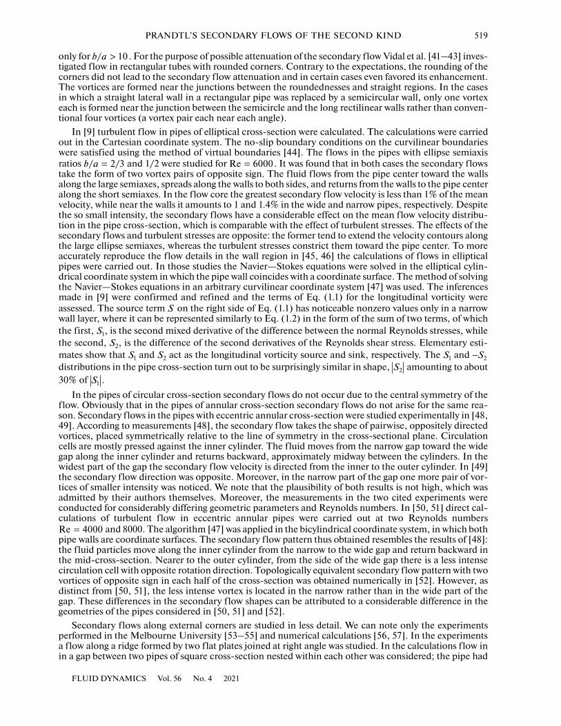
four internal and four external 90° corners. Although the Reynolds numbers in the calculations and exper-iments were considerably different, the results concerning the secondary f low features in the vicinity ofthe external corner are in qualitative agreement. In Fig. 7 we have plotted that mean velocity distributionand the secondary f low streamlines in the pipe, whose cross-section has an external corner [58]. The sec-ondary f low in the vicinity of the external corner takes the shape of a pair of vortices placed symmetricallyrelative to the corner bisector. The f luid motion in the secondary f low is directed from the corner towardthe f low along the bisector and toward the corner along the walls, that is, it is opposite to the case of theinternal corner. Correspondingly, the velocity contours have characteristic convexities directed from thecorner toward the f low. In the vicinity of the external corner the secondary f low intensity amounts to5.25% of , which is considerably greater than the analogous intensity near the internal corners, where amaximum value is about 2%. In [57] the distributions of the terms and and the expressions for thelongitudinal vorticity production (1.2) were calculated. As in the vicinities of the internal angles, and turn out to be similar in value and opposite in sign. Their role in the vorticity generation changes in differentparts of the vicinity of the corner.
Secondary f lows in the channels with free surfaces have been actively studied in view of their obviousgeophysical importance. The secondary f lows are associated with the zones of f luid elevation and lower-ing that comprise the entire f low thickness. In the full-scale conditions the secondary f lows have a con-siderable effect on gas and heat transfer and the self-aeration on the free surface. Thanks to the transportof bottom deposits by secondary f lows, the bottom shape changes and the bottom roughness becomesinhomogeneous, with the formation of longitudinal ridges and depressions, which enhances the second-ary f lows and ultimately leads to the generation of a chain of longitudinal vortices with alternate directionof rotation in the channel width. For this reason, the greatest attention is given to an investigation of f lowsin channels with a rough bottom in the presence of inhomogeneities of different type in the bottom rough-ness distributions [59–64].
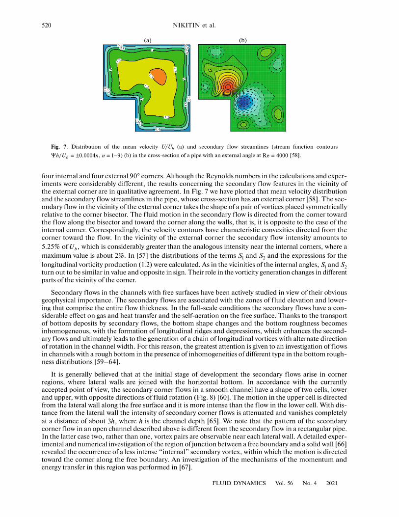
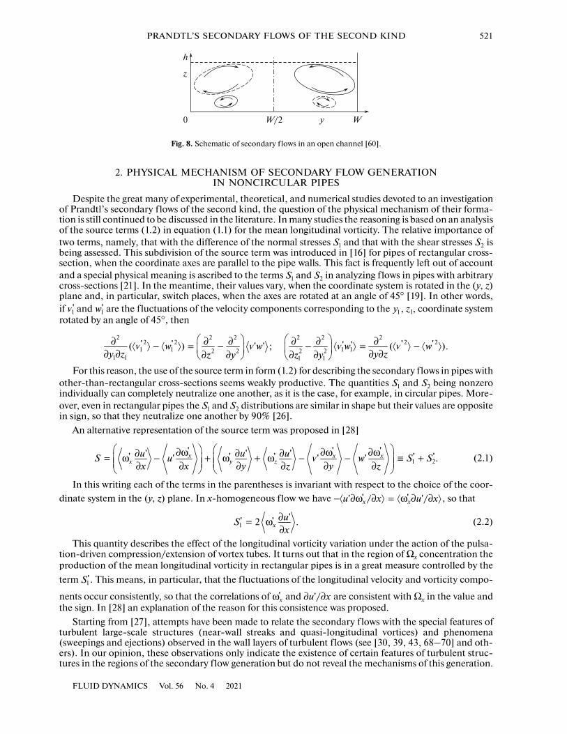
It is generally believed that at the initial stage of development the secondary f lows arise in cornerregions, where lateral walls are joined with the horizontal bottom. In accordance with the currentlyaccepted point of view, the secondary corner f lows in a smooth channel have a shape of two cells, lowerand upper, with opposite directions of f luid rotation (Fig. 8) [60]. The motion in the upper cell is directedfrom the lateral wall along the free surface and it is more intense than the f low in the lower cell. With dis-tance from the lateral wall the intensity of secondary corner f lows is attenuated and vanishes completelyat a distance of about , where is the channel depth [65]. We note that the pattern of the secondarycorner f low in an open channel described above is different from the secondary f low in a rectangular pipe.In the latter case two, rather than one, vortex pairs are observable near each lateral wall. A detailed exper-imental and numerical investigation of the region of junction between a free boundary and a solid wall [66]revealed the occurrence of a less intense “internal” secondary vortex, within which the motion is directedtoward the corner along the free boundary. An investigation of the mechanisms of the momentum andenergy transfer in this region was performed in [67].
bU1S 2S
1S 2S
3h h
FLUID DYNAMICS Vol. 56 No. 4 2021
PRANDTL’S SECONDARY FLOWS OF THE SECOND KIND 521
Fig. 8. Schematic of secondary f lows in an open channel [60].
h
z
0 W/2 Wy
2. PHYSICAL MECHANISM OF SECONDARY FLOW GENERATIONIN NONCIRCULAR PIPES
Despite the great many of experimental, theoretical, and numerical studies devoted to an investigationof Prandtl’s secondary f lows of the second kind, the question of the physical mechanism of their forma-tion is still continued to be discussed in the literature. In many studies the reasoning is based on an analysisof the source terms (1.2) in equation (1.1) for the mean longitudinal vorticity. The relative importance oftwo terms, namely, that with the difference of the normal stresses and that with the shear stresses isbeing assessed. This subdivision of the source term was introduced in [16] for pipes of rectangular cross-section, when the coordinate axes are parallel to the pipe walls. This fact is frequently left out of accountand a special physical meaning is ascribed to the terms and in analyzing f lows in pipes with arbitrarycross-sections [21]. In the meantime, their values vary, when the coordinate system is rotated in the (y, z)plane and, in particular, switch places, when the axes are rotated at an angle of 45° [19]. In other words,if and are the f luctuations of the velocity components corresponding to the , z1, coordinate systemrotated by an angle of 45°, then
For this reason, the use of the source term in form (1.2) for describing the secondary f lows in pipes withother-than-rectangular cross-sections seems weakly productive. The quantities and being nonzeroindividually can completely neutralize one another, as it is the case, for example, in circular pipes. More-over, even in rectangular pipes the and distributions are similar in shape but their values are oppositein sign, so that they neutralize one another by 90% [26].
An alternative representation of the source term was proposed in [28]
(2.1)
In this writing each of the terms in the parentheses is invariant with respect to the choice of the coor-dinate system in the (y, z) plane. In x-homogeneous f low we have , so that
(2.2)
This quantity describes the effect of the longitudinal vorticity variation under the action of the pulsa-tion-driven compression/extension of vortex tubes. It turns out that in the region of Ωx concentration theproduction of the mean longitudinal vorticity in rectangular pipes is in a great measure controlled by theterm . This means, in particular, that the f luctuations of the longitudinal velocity and vorticity compo-
nents occur consistently, so that the correlations of and are consistent with Ωx in the value andthe sign. In [28] an explanation of the reason for this consistence was proposed.
Starting from [27], attempts have been made to relate the secondary f lows with the special features ofturbulent large-scale structures (near-wall streaks and quasi-longitudinal vortices) and phenomena(sweepings and ejections) observed in the wall layers of turbulent f lows (see [30, 39, 43, 68–70] and oth-ers). In our opinion, these observations only indicate the existence of certain features of turbulent struc-tures in the regions of the secondary f low generation but do not reveal the mechanisms of this generation.
1S 2S
1S 2S
1'v 1'w 1y
∂ ∂ ∂ ∂ ∂ ∂ − = − ; − = − ∂ ∂ ∂ ∂∂ ∂ ∂ ∂
2 2 2 2 2 22 2 2 2
1 1 1 12 2 2 21 1 1 1
' ' ' '' '( ) ' ' ( ).w w w wy z y zz y z y
v v v v
1S 2S
1S 2S
∂ω ∂ω ∂ω∂ ∂ ∂= ω − + ω + ω − − ≡ + ∂ ∂ ∂ ∂ ∂ ∂ 1 2
' ' '' ' '' ' ' ' '' ' ' .x x xx y z
u u uS u w S Sx x y z y z
v
− ∂ω ∂ = ω ∂ ∂ ' '' / '/x xu x u x
∂= ω∂1
'' '2 .xuSx
1'S
ω'x ∂ ∂'/u x
FLUID DYNAMICS Vol. 56 No. 4 2021
522 NIKITIN et al.
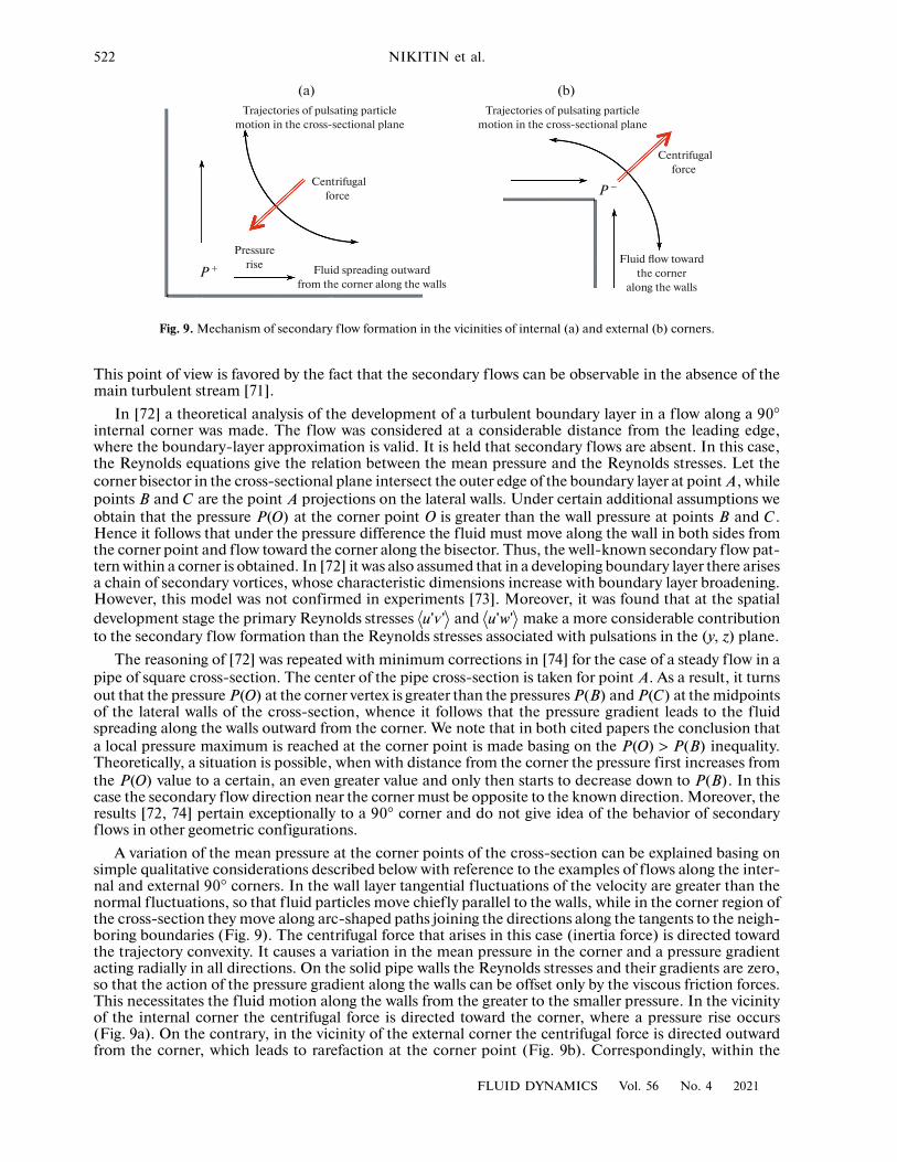
Fig. 9. Mechanism of secondary f low formation in the vicinities of internal (a) and external (b) corners.
Trajectories of pulsating particlemotion in the cross-sectional plane
Trajectories of pulsating particlemotion in the cross-sectional plane
(a) (b)
Centrifugalforce
Centrifugalforce
P �
P Pressure
rise Fluid spreading outwardfrom the corner along the walls
Fluid flow towardthe corner
along the walls
This point of view is favored by the fact that the secondary f lows can be observable in the absence of themain turbulent stream [71].
In [72] a theoretical analysis of the development of a turbulent boundary layer in a f low along a 90°internal corner was made. The f low was considered at a considerable distance from the leading edge,where the boundary-layer approximation is valid. It is held that secondary f lows are absent. In this case,the Reynolds equations give the relation between the mean pressure and the Reynolds stresses. Let thecorner bisector in the cross-sectional plane intersect the outer edge of the boundary layer at point , whilepoints and are the point projections on the lateral walls. Under certain additional assumptions weobtain that the pressure at the corner point O is greater than the wall pressure at points and .Hence it follows that under the pressure difference the f luid must move along the wall in both sides fromthe corner point and flow toward the corner along the bisector. Thus, the well-known secondary f low pat-tern within a corner is obtained. In [72] it was also assumed that in a developing boundary layer there arisesa chain of secondary vortices, whose characteristic dimensions increase with boundary layer broadening.However, this model was not confirmed in experiments [73]. Moreover, it was found that at the spatialdevelopment stage the primary Reynolds stresses and make a more considerable contributionto the secondary f low formation than the Reynolds stresses associated with pulsations in the (y, z) plane.
The reasoning of [72] was repeated with minimum corrections in [74] for the case of a steady f low in apipe of square cross-section. The center of the pipe cross-section is taken for point . As a result, it turnsout that the pressure at the corner vertex is greater than the pressures and at the midpointsof the lateral walls of the cross-section, whence it follows that the pressure gradient leads to the f luidspreading along the walls outward from the corner. We note that in both cited papers the conclusion thata local pressure maximum is reached at the corner point is made basing on the inequality.Theoretically, a situation is possible, when with distance from the corner the pressure first increases fromthe value to a certain, an even greater value and only then starts to decrease down to . In thiscase the secondary f low direction near the corner must be opposite to the known direction. Moreover, theresults [72, 74] pertain exceptionally to a 90° corner and do not give idea of the behavior of secondaryflows in other geometric configurations.
A variation of the mean pressure at the corner points of the cross-section can be explained basing onsimple qualitative considerations described below with reference to the examples of f lows along the inter-nal and external 90° corners. In the wall layer tangential f luctuations of the velocity are greater than thenormal f luctuations, so that f luid particles move chiefly parallel to the walls, while in the corner region ofthe cross-section they move along arc-shaped paths joining the directions along the tangents to the neigh-boring boundaries (Fig. 9). The centrifugal force that arises in this case (inertia force) is directed towardthe trajectory convexity. It causes a variation in the mean pressure in the corner and a pressure gradientacting radially in all directions. On the solid pipe walls the Reynolds stresses and their gradients are zero,so that the action of the pressure gradient along the walls can be offset only by the viscous friction forces.This necessitates the f luid motion along the walls from the greater to the smaller pressure. In the vicinityof the internal corner the centrifugal force is directed toward the corner, where a pressure rise occurs(Fig. 9a). On the contrary, in the vicinity of the external corner the centrifugal force is directed outwardfrom the corner, which leads to rarefaction at the corner point (Fig. 9b). Correspondingly, within the
AB C A
( )P O B C
v' 'u ' 'u w
A( )P O ( )P B ( )P C
>( ) ( )P O P B
( )P O ( )P B
FLUID DYNAMICS Vol. 56 No. 4 2021
PRANDTL’S SECONDARY FLOWS OF THE SECOND KIND 523
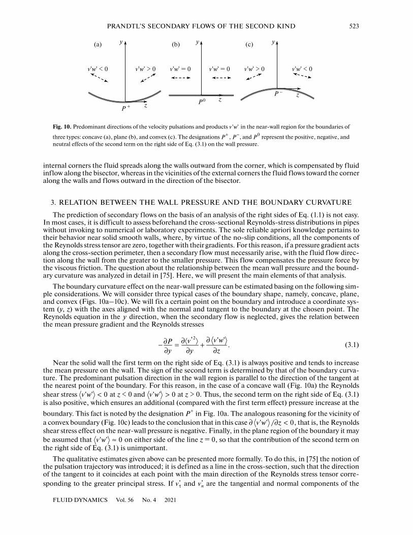
Fig. 10. Predominant directions of the velocity pulsations and products in the near-wall region for the boundaries of
three types: concave (a), plane (b), and convex (c). The designations , , and represent the positive, negative, andneutral effects of the second term on the right side of Eq. (3.1) on the wall pressure.
P +
P �
P 0
zz
z
y y y
v'w' < 0 v'w' > 0
(a) (b) (c)
v'w' = 0 v'w' = 0 v'w' > 0 v'w' < 0
v ' 'w+P −P 0P
internal corners the f luid spreads along the walls outward from the corner, which is compensated by f luidinflow along the bisector, whereas in the vicinities of the external corners the f luid f lows toward the corneralong the walls and flows outward in the direction of the bisector.
3. RELATION BETWEEN THE WALL PRESSURE AND THE BOUNDARY CURVATURE
The prediction of secondary f lows on the basis of an analysis of the right sides of Eq. (1.1) is not easy.In most cases, it is difficult to assess beforehand the cross-sectional Reynolds-stress distributions in pipeswithout invoking to numerical or laboratory experiments. The sole reliable apriori knowledge pertains totheir behavior near solid smooth walls, where, by virtue of the no-slip conditions, all the components ofthe Reynolds stress tensor are zero, together with their gradients. For this reason, if a pressure gradient actsalong the cross-section perimeter, then a secondary f low must necessarily arise, with the f luid f low direc-tion along the wall from the greater to the smaller pressure. This f low compensates the pressure force bythe viscous friction. The question about the relationship between the mean wall pressure and the bound-ary curvature was analyzed in detail in [75]. Here, we will present the main elements of that analysis.
The boundary curvature effect on the near-wall pressure can be estimated basing on the following sim-ple considerations. We will consider three typical cases of the boundary shape, namely, concave, plane,and convex (Figs. 10a–10c). We will fix a certain point on the boundary and introduce a coordinate sys-tem (y, z) with the axes aligned with the normal and tangent to the boundary at the chosen point. TheReynolds equation in the direction, when the secondary f low is neglected, gives the relation betweenthe mean pressure gradient and the Reynolds stresses
(3.1)
Near the solid wall the first term on the right side of Eq. (3.1) is always positive and tends to increasethe mean pressure on the wall. The sign of the second term is determined by that of the boundary curva-ture. The predominant pulsation direction in the wall region is parallel to the direction of the tangent atthe nearest point of the boundary. For this reason, in the case of a concave wall (Fig. 10a) the Reynoldsshear stress at z < 0 and at z > 0. Thus, the second term on the right side of Eq. (3.1)is also positive, which ensures an additional (compared with the first term effect) pressure increase at theboundary. This fact is noted by the designation in Fig. 10a. The analogous reasoning for the vicinity ofa convex boundary (Fig. 10c) leads to the conclusion that in this case , that is, the Reynoldsshear stress effect on the near-wall pressure is negative. Finally, in the plane region of the boundary it maybe assumed that on either side of the line z = 0, so that the contribution of the second term onthe right side of Eq. (3.1) is unimportant.
The qualitative estimates given above can be presented more formally. To do this, in [75] the notion ofthe pulsation trajectory was introduced; it is defined as a line in the cross-section, such that the directionof the tangent to it coincides at each point with the main direction of the Reynolds stress tensor corre-sponding to the greater principal stress. If and are the tangential and normal components of the
y
∂∂ ∂− = +∂ ∂ ∂
2' ' '.
wPy y z
vv
<v' ' 0w >v' ' 0w
+P∂ ∂ <v' ' / 0w z
≈v' ' 0w
τv ' v 'n
FLUID DYNAMICS Vol. 56 No. 4 2021
524 NIKITIN et al.
velocity f luctuation components along the trajectory, then and . It was proved thatan any point on the trajectory
(3.2)
Here, n is the principal normal and is the radius of curvature of the trajectory. The first term on theright side of Eq. (3.2) indicates that the pressure variation along the normal is opposite to the normal stressvariation in the same direction and does not depend on the curvature of the pulsation trajectory. The sec-ond term is always positive, whence it follows that the f luctuating motion along a curved trajectoryincreases the pressure in the direction of the trajectory convexity. This increase is proportional to the tra-jectory curvature.
The curving of the pulsation trajectories takes place near curved walls, where and ,d being the distance to the wall. As , and it may be assumed that the pulsation trajec-tory curvature is similar in value with the wall curvature. It is reasonable to suggest that the pulsation tra-jectory curvature retains the sign even at a certain distance from the wall, so that the effect of the secondterm on the right side of Eq. (3.2) leads to a finite variation in the wall pressure. Thus, with variation inthe wall curvature a proportional variation of the pressure might be expected in the neighboring regions ofthe pipe cross-section perimeter: with increase in the wall curvature the pressure increases on concavewalls and decreases on convex walls. As noted above, the Reynolds stresses cannot balance out the pres-sure force action along the wall, so that a secondary f low must arise. In accordance with the above, themotion in the secondary f low must be directed from the greater toward the smaller curvature along con-cave walls and vice versa along the convex walls.
Obviously that the curving of the pulsation trajectories occurs also in corner regions. The family of pul-sation trajectories in a pipe of square cross-section for [28] is presented in Fig. 11a. The radiusof curvature of the pulsation trajectories is zero directly at the corner point and increases with distancefrom it. A noticeable curving of the trajectories can be observable in the region, where . In thesame region there exists a considerable anisotropy of normal stresses, which makes a contribution to thesecond term on the right side of Eq. (3.2). In Fig. 11b the pressure field is presented, together with the sec-ondary f low streamlines. Precisely in the zone of curving of the pulsation trajectories an additional wallpressure rise is observable, as compared with the boundary regions, more distant from the corner. Beyondthis region the pulsation trajectories are parallel to the walls and it is only the first term on the right sideof Eq. (3.2) that contributes to the wall pressure rise. In the internal corners both terms on the right sideof Eq. (3.2) are positive and their effects are added. In the vicinities of the external corners the pulsationtrajectories are directed outward from the corner by their convexities, so that the second term on the rightside of Eq. (3.2) tends to diminish the pressure in the corner. This leads to rarefaction (relative to the sur-rounding regions of the perimeter) in the corner region and a secondary f low directed along the wallstoward the corner and along the bisector outward from the corner.
4. PREDICTION AND EXPLANATION OF THE SECONDARY FLOW SHAPEIN NONCIRCULAR PIPES
The arguments and estimates of the preceding section concerning the relation between the curvatureof the pipe cross-section boundary and the mean pressure and the direction of the generated secondaryflow can be formulated in the form of the following principle. The secondary f low along the pipe walls isdirected from the points of local pressure maximum to those of local pressure minimum. The conse-quence of this principle is the f luid inflow from the external f low toward the points of local pressure max-ima on the walls and, contrariwise, the f luid return from the walls into the external f low from the pointsof local pressure minimum. In the vicinity of any extremum the streamlines take the form presented inFig. 12. At the points of local extrema of the boundary curvature the pressure extrema of the same type arereached on concave walls and of the opposite type on convex walls.
This principle can be used for approximately estimating and predicting the shape of the secondaryflows occurring in one or another version of the pipe cross-section. For this purpose, an attempt shouldbe made to determine the points of local pressure extrema on the pipe cross-section boundary basing onan analysis of the boundary curvature, symmetry conditions, or some other considerations. Two extremaof the same type cannot be next to one another on an interval of a boundary but they must necessarily beseparated by at least one extremum of the opposite type.
τ > v v2 2' 'n τ =' ' 0nv v
τ∂ − ∂− = +∂ ∂
2 2 2' ' '.n nP
n n Rv v v
R
τ v ∼
2 2' d v ∼
2 4'n d→ 0d τ �
2 2' 'nv v
τ =Re 150
+ +, < 50y z
FLUID DYNAMICS Vol. 56 No. 4 2021

PRANDTL’S SECONDARY FLOWS OF THE SECOND KIND 525
Fig. 11. Directions of the tangents to pulsation trajectories in a square pipe (a) and mean pressure field and secondaryflow streamlines (b) at . The vector lengths in panel (a) are proportional to the anisotropy degree of the normalstresses . A quarter pipe cross-section is presented.
150z+
100
50
0
150z+
y+y+
100
50
050 100 150 50 100 150
(a) (b)
τ =Re 150
τ τ − + v v v v2 2 2 2( )/( )' ' ' 'n n
Fig. 12. Secondary f low streamline shapes in the vicinities of the points of local minimum and maximum of themean wall pressure.
P � P
+
−P +P
Fig. 13. Mean pressure distribution (a) and secondary f low streamlines (b) in a pipe with the cross-section in the shapeof a circular sector with the vertex angle of 90° [76].
A
C C '
B 'B
D
A(a) (b)
C C '
B 'B
D
We will try to apply the receipt presented above to certain particular cases. In Figs. 13 and 14 we havepresented the pressure distributions and the secondary f low streamlines in the pipes with cross-sectionsin the shape of a circular sector with the vertex angles 90° and 270° obtained in the DNS calculations at
[76]. Here, Ub is the mean velocity and is the hydraulic diameter.
An apriori analysis of the pipe cross-section with the vertex angle 90° (Fig. 13) allows one to make thefollowing conclusions. For the reasons described above, in three internal corners A, , and the pressureis greater than on the surrounding intervals of the perimeter. On the rectilinear intervals and theremust be points of local pressure minimum; we will denote them as and . Any variations in the bound-ary curvature or any other reasons indicating the presence of other extrema are absent from these intervals.
= ν ≈Re / 2800b hU D hD
B 'BAB 'AB
C 'C
FLUID DYNAMICS Vol. 56 No. 4 2021
526 NIKITIN et al.
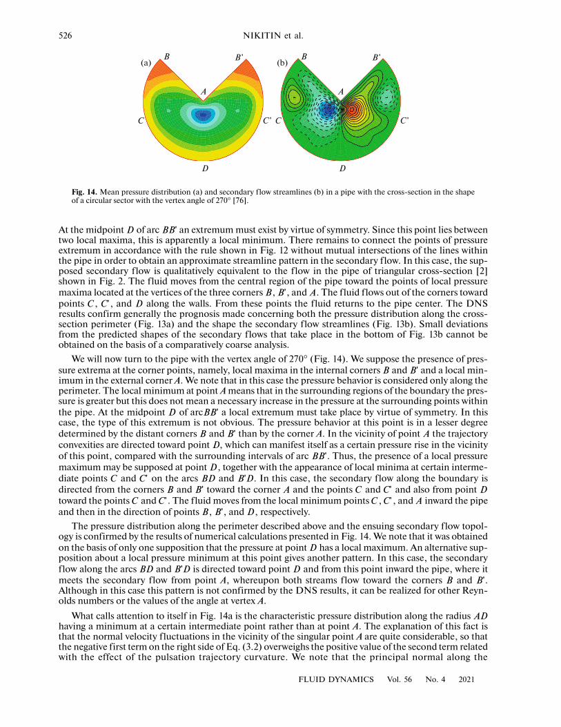
Fig. 14. Mean pressure distribution (a) and secondary f low streamlines (b) in a pipe with the cross-section in the shapeof a circular sector with the vertex angle of 270° [76].
A
C C '
B 'B
D
A
C C '
B 'B
D
(a) (b)
At the midpoint of arc an extremum must exist by virtue of symmetry. Since this point lies betweentwo local maxima, this is apparently a local minimum. There remains to connect the points of pressureextremum in accordance with the rule shown in Fig. 12 without mutual intersections of the lines withinthe pipe in order to obtain an approximate streamline pattern in the secondary f low. In this case, the sup-posed secondary f low is qualitatively equivalent to the f low in the pipe of triangular cross-section [2]shown in Fig. 2. The f luid moves from the central region of the pipe toward the points of local pressuremaxima located at the vertices of the three corners , , and . The f luid f lows out of the corners towardpoints , , and along the walls. From these points the f luid returns to the pipe center. The DNSresults confirm generally the prognosis made concerning both the pressure distribution along the cross-section perimeter (Fig. 13a) and the shape the secondary f low streamlines (Fig. 13b). Small deviationsfrom the predicted shapes of the secondary f lows that take place in the bottom of Fig. 13b cannot beobtained on the basis of a comparatively coarse analysis.
We will now turn to the pipe with the vertex angle of 270° (Fig. 14). We suppose the presence of pres-sure extrema at the corner points, namely, local maxima in the internal corners and and a local min-imum in the external corner A. We note that in this case the pressure behavior is considered only along theperimeter. The local minimum at point A means that in the surrounding regions of the boundary the pres-sure is greater but this does not mean a necessary increase in the pressure at the surrounding points withinthe pipe. At the midpoint of arc a local extremum must take place by virtue of symmetry. In thiscase, the type of this extremum is not obvious. The pressure behavior at this point is in a lesser degreedetermined by the distant corners and than by the corner A. In the vicinity of point the trajectoryconvexities are directed toward point , which can manifest itself as a certain pressure rise in the vicinityof this point, compared with the surrounding intervals of arc . Thus, the presence of a local pressuremaximum may be supposed at point , together with the appearance of local minima at certain interme-diate points and on the arcs and . In this case, the secondary f low along the boundary isdirected from the corners and toward the corner and the points and and also from point toward the points and . The f luid moves from the local minimum points , , and inward the pipeand then in the direction of points , , and , respectively.
The pressure distribution along the perimeter described above and the ensuing secondary f low topol-ogy is confirmed by the results of numerical calculations presented in Fig. 14. We note that it was obtainedon the basis of only one supposition that the pressure at point has a local maximum. An alternative sup-position about a local pressure minimum at this point gives another pattern. In this case, the secondaryflow along the arcs and is directed toward point and from this point inward the pipe, where itmeets the secondary f low from point A, whereupon both streams flow toward the corners and .Although in this case this pattern is not confirmed by the DNS results, it can be realized for other Reyn-olds numbers or the values of the angle at vertex A.
What calls attention to itself in Fig. 14a is the characteristic pressure distribution along the radius having a minimum at a certain intermediate point rather than at point A. The explanation of this fact isthat the normal velocity f luctuations in the vicinity of the singular point A are quite considerable, so thatthe negative first term on the right side of Eq. (3.2) overweighs the positive value of the second term relatedwith the effect of the pulsation trajectory curvature. We note that the principal normal along the
D 'BB
B 'B AC 'C D
B 'B
D 'BB
B 'B AD
'BBD
C 'C BD 'B DB 'B A C 'C D
C 'C C 'C AB 'B D
D
BD 'B D DB 'B
AD
FLUID DYNAMICS Vol. 56 No. 4 2021
PRANDTL’S SECONDARY FLOWS OF THE SECOND KIND 527
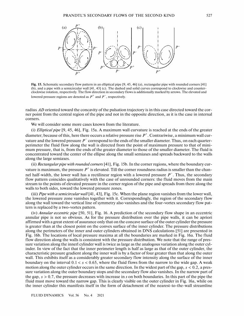
Fig. 15. Schematic secondary f low pattern in an elliptical pipe [9, 45, 46] (a), rectangular pipe with rounded corners [41](b), and a pipe with a semicircular wall [41, 43] (c). The dashed and solid curves correspond to clockwise and counter-clockwise rotation, respectively. The flow direction in secondary f lows is additionally marked by arrows. The elevated andlowered pressure regions are denoted as and , respectively.
P � P
�
P � P
�P � P
�
P �
P + P
+P
+ P +
P +
(a) (b) (c)
+P −P
radius oriented toward the concavity of the pulsation trajectory is in this case directed toward the cor-ner point from the central region of the pipe and not in the opposite direction, as it is the case in internalcorners.
We will consider some more cases known from the literature.(i) Elliptical pipe [9, 45, 46], Fig. 15a. A maximum wall curvature is reached at the ends of the greater
diameter; because of this, here there occurs a relative pressure rise . Contrariwise, a minimum wall cur-vature and the lowered pressure correspond to the ends of the smaller diameter. Thus, on each quarter-perimeter the f luid f low along the wall is directed from the point of maximum pressure to that of mini-mum pressure, that is, from the ends of the greater diameter to those of the smaller diameter. The f luid isconcentrated toward the center of the ellipse along the small semiaxes and spreads backward to the wallsalong the large semiaxes.
(ii) Rectangular pipe with rounded corners [41], Fig. 15b. In the corner regions, where the boundary cur-vature is maximum, the pressure is elevated. Till the corner roundness radius is smaller than the chan-nel half-width, the lower wall has a rectilinear region with a lowered pressure . Thus, the secondaryflow pattern coincides qualitatively with the case of unrounded corners: the f luid moves from the mainstream to the points of elevated pressure in the corner region of the pipe and spreads from there along thewalls to both sides, toward the lowered pressure zones.
(iii) Pipe with a semicircular wall [41, 43], Fig. 15c. When the plane region vanishes from the lower wall,the lowered pressure zone vanishes together with it. Correspondingly, the region of the secondary f lowalong the wall toward the vertical line of symmetry also vanishes and the four-vortex secondary f low pat-tern is replaced by a two-vortex pattern.
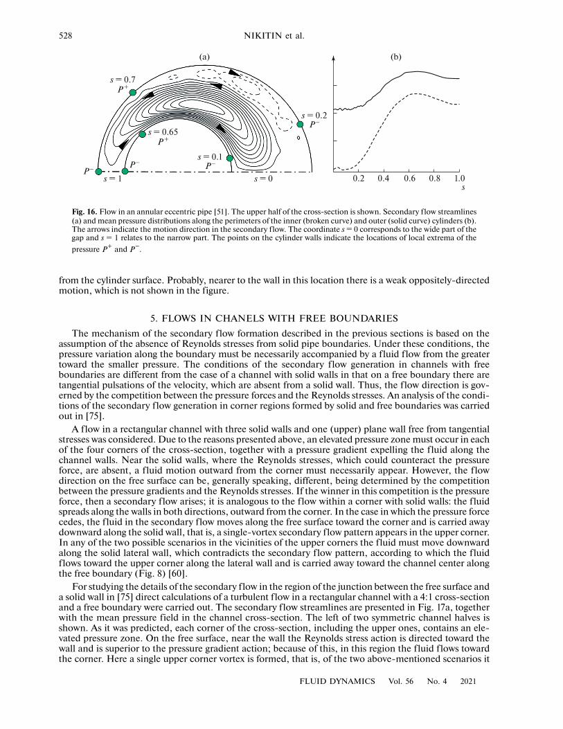
(iv) Annular eccentric pipe [50, 51], Fig. 16. A prediction of the secondary f low shape in an eccentricannular pipe is not so obvious. As for the pressure distribution over the pipe walls, it can be aprioriaffirmed with a great extent of assurance only that on the concave surface of the outer cylinder the pressureis greater than at the closest point on the convex surface of the inner cylinder. The pressure distributionsalong the perimeters of the inner and outer cylinders obtained in DNS calculations [51] are presented inFig. 16b. The locations of local pressure maxima at all the boundaries are marked in Fig. 16a. The f luidflow direction along the walls is consistent with the pressure distribution. We note that the range of pres-sure variation along the innerl cylinder wall is twice as large as the analogous variation along the outer cyl-inder. In view of the fact that the inner perimeter length is half as large as that of the outer cylinder, thecharacteristic pressure gradient along the inner wall is by a factor of four greater than that along the outerwall. This exhibits itself as a considerably greater secondary f low intensity along the surface of the innerboundary on the interval , where the f luid f lows from the narrow to the wide gap. A weakmotion along the outer cylinder occurs in the same direction. In the widest part of the gap, , a pres-sure variation along the outer boundary stops and the secondary f low also vanishes. In the narrow part ofthe gap, , the pressure decreases with increase in s on both boundaries. In this part of the pipe thefluid must move toward the narrow gap. This is clearly visible on the outer cylinder in Fig. 16a, while onthe inner cylinder this manifests itself in the form of detachment of the nearest-to-the-wall streamline
AD
+P−P
+P−P
. < < .0 1 0 65s< .0 2s
> .0 7s
FLUID DYNAMICS Vol. 56 No. 4 2021
528 NIKITIN et al.
Fig. 16. Flow in an annular eccentric pipe [51]. The upper half of the cross-section is shown. Secondary f low streamlines(a) and mean pressure distributions along the perimeters of the inner (broken curve) and outer (solid curve) cylinders (b).The arrows indicate the motion direction in the secondary f low. The coordinate s = 0 corresponds to the wide part of thegap and s = 1 relates to the narrow part. The points on the cylinder walls indicate the locations of local extrema of thepressure and .
s = 0.7P
+
s = 0.65P
+
s = 0.1P −
s = 0.2P −
0.2 0.4 0.6 0.8 1.0s
s = 1 s = 0P − P
−
(a) (b)
+P −P
from the cylinder surface. Probably, nearer to the wall in this location there is a weak oppositely-directedmotion, which is not shown in the figure.
5. FLOWS IN CHANELS WITH FREE BOUNDARIESThe mechanism of the secondary f low formation described in the previous sections is based on the
assumption of the absence of Reynolds stresses from solid pipe boundaries. Under these conditions, thepressure variation along the boundary must be necessarily accompanied by a f luid f low from the greatertoward the smaller pressure. The conditions of the secondary f low generation in channels with freeboundaries are different from the case of a channel with solid walls in that on a free boundary there aretangential pulsations of the velocity, which are absent from a solid wall. Thus, the f low direction is gov-erned by the competition between the pressure forces and the Reynolds stresses. An analysis of the condi-tions of the secondary f low generation in corner regions formed by solid and free boundaries was carriedout in [75].
A flow in a rectangular channel with three solid walls and one (upper) plane wall free from tangentialstresses was considered. Due to the reasons presented above, an elevated pressure zone must occur in eachof the four corners of the cross-section, together with a pressure gradient expelling the f luid along thechannel walls. Near the solid walls, where the Reynolds stresses, which could counteract the pressureforce, are absent, a f luid motion outward from the corner must necessarily appear. However, the f lowdirection on the free surface can be, generally speaking, different, being determined by the competitionbetween the pressure gradients and the Reynolds stresses. If the winner in this competition is the pressureforce, then a secondary f low arises; it is analogous to the f low within a corner with solid walls: the f luidspreads along the walls in both directions, outward from the corner. In the case in which the pressure forcecedes, the f luid in the secondary f low moves along the free surface toward the corner and is carried awaydownward along the solid wall, that is, a single-vortex secondary f low pattern appears in the upper corner.In any of the two possible scenarios in the vicinities of the upper corners the f luid must move downwardalong the solid lateral wall, which contradicts the secondary f low pattern, according to which the f luidflows toward the upper corner along the lateral wall and is carried away toward the channel center alongthe free boundary (Fig. 8) [60].
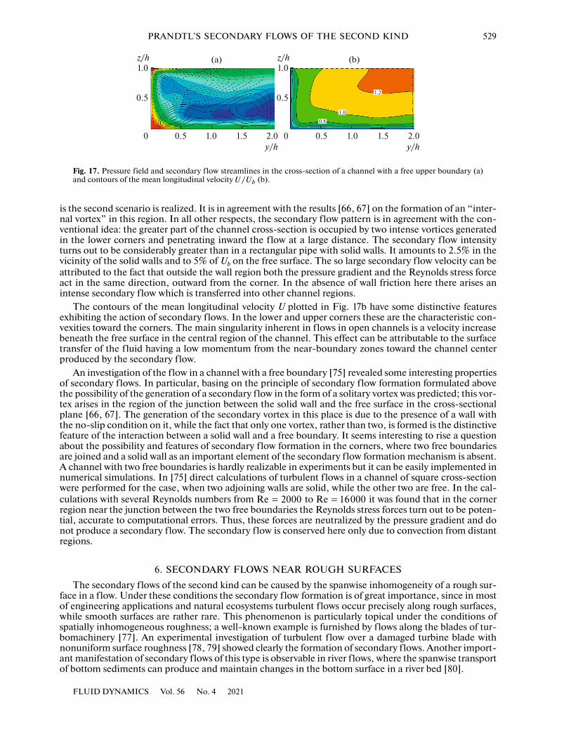
For studying the details of the secondary f low in the region of the junction between the free surface anda solid wall in [75] direct calculations of a turbulent f low in a rectangular channel with a 4:1 cross-sectionand a free boundary were carried out. The secondary f low streamlines are presented in Fig. 17a, togetherwith the mean pressure field in the channel cross-section. The left of two symmetric channel halves isshown. As it was predicted, each corner of the cross-section, including the upper ones, contains an ele-vated pressure zone. On the free surface, near the wall the Reynolds stress action is directed toward thewall and is superior to the pressure gradient action; because of this, in this region the f luid f lows towardthe corner. Here a single upper corner vortex is formed, that is, of the two above-mentioned scenarios it
FLUID DYNAMICS Vol. 56 No. 4 2021
PRANDTL’S SECONDARY FLOWS OF THE SECOND KIND 529
Fig. 17. Pressure field and secondary f low streamlines in the cross-section of a channel with a free upper boundary (a)and contours of the mean longitudinal velocity (b).
0.5
0.5 1.0 1.5 2.0
1.0(a) (b)z/h
y/h0
0.5
0.5 1.0 1.5 2.0
1.0z/h
y/h0
���������
���������
���������
/ bU U
is the second scenario is realized. It is in agreement with the results [66, 67] on the formation of an “inter-nal vortex” in this region. In all other respects, the secondary f low pattern is in agreement with the con-ventional idea: the greater part of the channel cross-section is occupied by two intense vortices generatedin the lower corners and penetrating inward the f low at a large distance. The secondary f low intensityturns out to be considerably greater than in a rectangular pipe with solid walls. It amounts to 2.5% in thevicinity of the solid walls and to 5% of Ub on the free surface. The so large secondary f low velocity can beattributed to the fact that outside the wall region both the pressure gradient and the Reynolds stress forceact in the same direction, outward from the corner. In the absence of wall friction here there arises anintense secondary f low which is transferred into other channel regions.
The contours of the mean longitudinal velocity U plotted in Fig. 17b have some distinctive featuresexhibiting the action of secondary f lows. In the lower and upper corners these are the characteristic con-vexities toward the corners. The main singularity inherent in f lows in open channels is a velocity increasebeneath the free surface in the central region of the channel. This effect can be attributable to the surfacetransfer of the f luid having a low momentum from the near-boundary zones toward the channel centerproduced by the secondary f low.
An investigation of the f low in a channel with a free boundary [75] revealed some interesting propertiesof secondary f lows. In particular, basing on the principle of secondary f low formation formulated abovethe possibility of the generation of a secondary f low in the form of a solitary vortex was predicted; this vor-tex arises in the region of the junction between the solid wall and the free surface in the cross-sectionalplane [66, 67]. The generation of the secondary vortex in this place is due to the presence of a wall withthe no-slip condition on it, while the fact that only one vortex, rather than two, is formed is the distinctivefeature of the interaction between a solid wall and a free boundary. It seems interesting to rise a questionabout the possibility and features of secondary f low formation in the corners, where two free boundariesare joined and a solid wall as an important element of the secondary f low formation mechanism is absent.A channel with two free boundaries is hardly realizable in experiments but it can be easily implemented innumerical simulations. In [75] direct calculations of turbulent f lows in a channel of square cross-sectionwere performed for the case, when two adjoining walls are solid, while the other two are free. In the cal-culations with several Reynolds numbers from to it was found that in the cornerregion near the junction between the two free boundaries the Reynolds stress forces turn out to be poten-tial, accurate to computational errors. Thus, these forces are neutralized by the pressure gradient and donot produce a secondary f low. The secondary f low is conserved here only due to convection from distantregions.
6. SECONDARY FLOWS NEAR ROUGH SURFACESThe secondary f lows of the second kind can be caused by the spanwise inhomogeneity of a rough sur-
face in a f low. Under these conditions the secondary f low formation is of great importance, since in mostof engineering applications and natural ecosystems turbulent f lows occur precisely along rough surfaces,while smooth surfaces are rather rare. This phenomenon is particularly topical under the conditions ofspatially inhomogeneous roughness; a well-known example is furnished by f lows along the blades of tur-bomachinery [77]. An experimental investigation of turbulent f low over a damaged turbine blade withnonuniform surface roughness [78, 79] showed clearly the formation of secondary f lows. Another import-ant manifestation of secondary f lows of this type is observable in river f lows, where the spanwise transportof bottom sediments can produce and maintain changes in the bottom surface in a river bed [80].
=Re 2000 =Re 16000
FLUID DYNAMICS Vol. 56 No. 4 2021
530 NIKITIN et al.
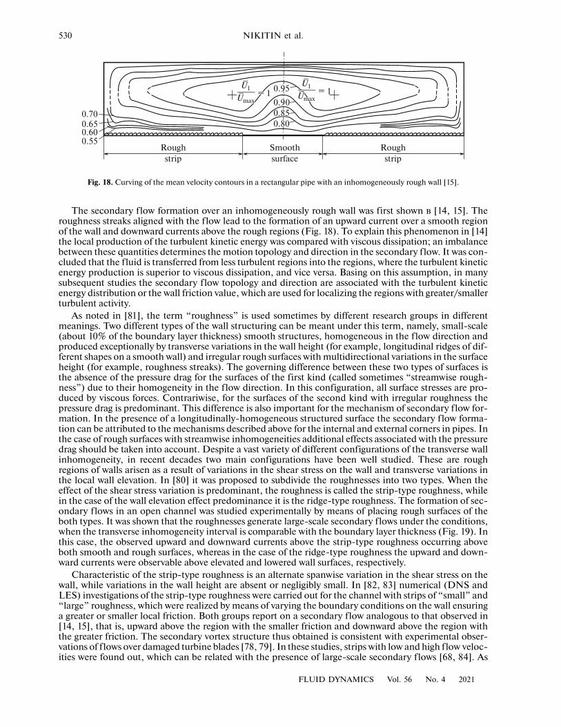
Fig. 18. Curving of the mean velocity contours in a rectangular pipe with an inhomogeneously rough wall [15].
0.70
0.600.55
0.800.800.80
0.900.900.900.950.950.95
0.850.850.85
Roughstrip
Roughstrip
Smoothsurface
0.65
= 1 = 1 = 1 ���� ���� ���� � � �
� � �U1U1U1
UmaxUmaxUmax = 1 = 1 = 1 ���� ���� ����
� � � � � �U1U1U1
UmaxUmaxUmax
The secondary f low formation over an inhomogeneously rough wall was first shown в [14, 15]. Theroughness streaks aligned with the f low lead to the formation of an upward current over a smooth regionof the wall and downward currents above the rough regions (Fig. 18). To explain this phenomenon in [14]the local production of the turbulent kinetic energy was compared with viscous dissipation; an imbalancebetween these quantities determines the motion topology and direction in the secondary f low. It was con-cluded that the f luid is transferred from less turbulent regions into the regions, where the turbulent kineticenergy production is superior to viscous dissipation, and vice versa. Basing on this assumption, in manysubsequent studies the secondary f low topology and direction are associated with the turbulent kineticenergy distribution or the wall friction value, which are used for localizing the regions with greater/smallerturbulent activity.
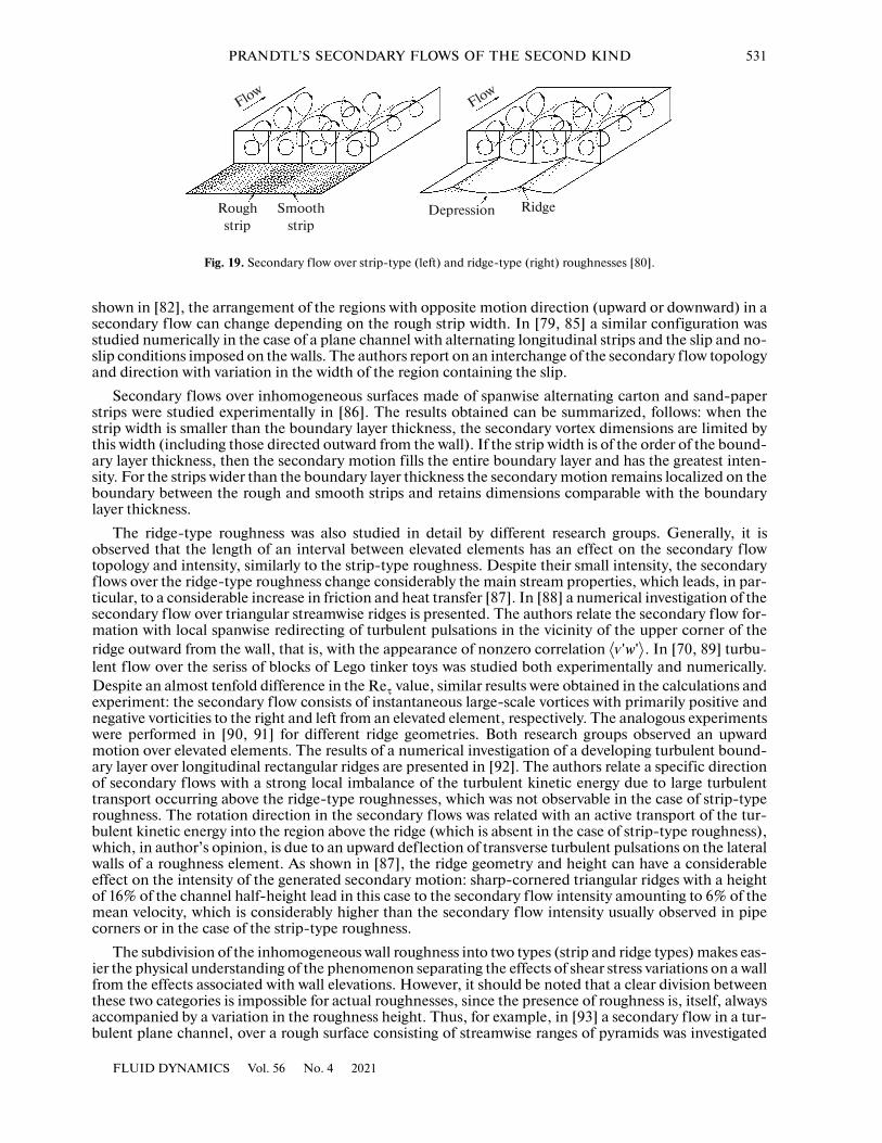
As noted in [81], the term “roughness” is used sometimes by different research groups in differentmeanings. Two different types of the wall structuring can be meant under this term, namely, small-scale(about 10% of the boundary layer thickness) smooth structures, homogeneous in the f low direction andproduced exceptionally by transverse variations in the wall height (for example, longitudinal ridges of dif-ferent shapes on a smooth wall) and irregular rough surfaces with multidirectional variations in the surfaceheight (for example, roughness streaks). The governing difference between these two types of surfaces isthe absence of the pressure drag for the surfaces of the first kind (called sometimes “streamwise rough-ness”) due to their homogeneity in the f low direction. In this configuration, all surface stresses are pro-duced by viscous forces. Contrariwise, for the surfaces of the second kind with irregular roughness thepressure drag is predominant. This difference is also important for the mechanism of secondary f low for-mation. In the presence of a longitudinally-homogeneous structured surface the secondary f low forma-tion can be attributed to the mechanisms described above for the internal and external corners in pipes. Inthe case of rough surfaces with streamwise inhomogeneities additional effects associated with the pressuredrag should be taken into account. Despite a vast variety of different configurations of the transverse wallinhomogeneity, in recent decades two main configurations have been well studied. These are roughregions of walls arisen as a result of variations in the shear stress on the wall and transverse variations inthe local wall elevation. In [80] it was proposed to subdivide the roughnesses into two types. When theeffect of the shear stress variation is predominant, the roughness is called the strip-type roughness, whilein the case of the wall elevation effect predominance it is the ridge-type roughness. The formation of sec-ondary f lows in an open channel was studied experimentally by means of placing rough surfaces of theboth types. It was shown that the roughnesses generate large-scale secondary f lows under the conditions,when the transverse inhomogeneity interval is comparable with the boundary layer thickness (Fig. 19). Inthis case, the observed upward and downward currents above the strip-type roughness occurring aboveboth smooth and rough surfaces, whereas in the case of the ridge-type roughness the upward and down-ward currents were observable above elevated and lowered wall surfaces, respectively.
Characteristic of the strip-type roughness is an alternate spanwise variation in the shear stress on thewall, while variations in the wall height are absent or negligibly small. In [82, 83] numerical (DNS andLES) investigations of the strip-type roughness were carried out for the channel with strips of “small” and“large” roughness, which were realized by means of varying the boundary conditions on the wall ensuringa greater or smaller local friction. Both groups report on a secondary f low analogous to that observed in[14, 15], that is, upward above the region with the smaller friction and downward above the region withthe greater friction. The secondary vortex structure thus obtained is consistent with experimental obser-vations of f lows over damaged turbine blades [78, 79]. In these studies, strips with low and high f low veloc-ities were found out, which can be related with the presence of large-scale secondary f lows [68, 84]. As
FLUID DYNAMICS Vol. 56 No. 4 2021
PRANDTL’S SECONDARY FLOWS OF THE SECOND KIND 531
Fig. 19. Secondary f low over strip-type (left) and ridge-type (right) roughnesses [80].
FlowFlow
Roughstrip
Smoothstrip
Depression Ridge
shown in [82], the arrangement of the regions with opposite motion direction (upward or downward) in asecondary f low can change depending on the rough strip width. In [79, 85] a similar configuration wasstudied numerically in the case of a plane channel with alternating longitudinal strips and the slip and no-slip conditions imposed on the walls. The authors report on an interchange of the secondary f low topologyand direction with variation in the width of the region containing the slip.
Secondary f lows over inhomogeneous surfaces made of spanwise alternating carton and sand-paperstrips were studied experimentally in [86]. The results obtained can be summarized, follows: when thestrip width is smaller than the boundary layer thickness, the secondary vortex dimensions are limited bythis width (including those directed outward from the wall). If the strip width is of the order of the bound-ary layer thickness, then the secondary motion fills the entire boundary layer and has the greatest inten-sity. For the strips wider than the boundary layer thickness the secondary motion remains localized on theboundary between the rough and smooth strips and retains dimensions comparable with the boundarylayer thickness.
The ridge-type roughness was also studied in detail by different research groups. Generally, it isobserved that the length of an interval between elevated elements has an effect on the secondary f lowtopology and intensity, similarly to the strip-type roughness. Despite their small intensity, the secondaryflows over the ridge-type roughness change considerably the main stream properties, which leads, in par-ticular, to a considerable increase in friction and heat transfer [87]. In [88] a numerical investigation of thesecondary f low over triangular streamwise ridges is presented. The authors relate the secondary f low for-mation with local spanwise redirecting of turbulent pulsations in the vicinity of the upper corner of theridge outward from the wall, that is, with the appearance of nonzero correlation . In [70, 89] turbu-lent f low over the seriss of blocks of Lego tinker toys was studied both experimentally and numerically.Despite an almost tenfold difference in the value, similar results were obtained in the calculations andexperiment: the secondary f low consists of instantaneous large-scale vortices with primarily positive andnegative vorticities to the right and left from an elevated element, respectively. The analogous experimentswere performed in [90, 91] for different ridge geometries. Both research groups observed an upwardmotion over elevated elements. The results of a numerical investigation of a developing turbulent bound-ary layer over longitudinal rectangular ridges are presented in [92]. The authors relate a specific directionof secondary f lows with a strong local imbalance of the turbulent kinetic energy due to large turbulenttransport occurring above the ridge-type roughnesses, which was not observable in the case of strip-typeroughness. The rotation direction in the secondary f lows was related with an active transport of the tur-bulent kinetic energy into the region above the ridge (which is absent in the case of strip-type roughness),which, in author’s opinion, is due to an upward deflection of transverse turbulent pulsations on the lateralwalls of a roughness element. As shown in [87], the ridge geometry and height can have a considerableeffect on the intensity of the generated secondary motion: sharp-cornered triangular ridges with a heightof 16% of the channel half-height lead in this case to the secondary f low intensity amounting to 6% of themean velocity, which is considerably higher than the secondary f low intensity usually observed in pipecorners or in the case of the strip-type roughness.
The subdivision of the inhomogeneous wall roughness into two types (strip and ridge types) makes eas-ier the physical understanding of the phenomenon separating the effects of shear stress variations on a wallfrom the effects associated with wall elevations. However, it should be noted that a clear division betweenthese two categories is impossible for actual roughnesses, since the presence of roughness is, itself, alwaysaccompanied by a variation in the roughness height. Thus, for example, in [93] a secondary f low in a tur-bulent plane channel, over a rough surface consisting of streamwise ranges of pyramids was investigated
v' 'w
τRe
FLUID DYNAMICS Vol. 56 No. 4 2021
532 NIKITIN et al.
numerically for different spacings between the ranges. An effect of the change in the secondary f low direc-tion was revealed with increase in the interval between the roughness ranges higher than the channelheight. For smaller intervals an upward motion occurs above roughness elements, which is consistent withthe secondary f lows over the ridge-type roughnesses, while at large spacings a downward motion arisesover the elements. Recently, in [94] it was shown that the rotation direction in the secondary f lows abovea wall with a roughness strip depends on the relative height of the mean level of the roughness strip (ele-vated or lowered). In that study three different levels of the mean height of the roughness strip were con-sidered. They corresponded to elevated (caused by deposits), submerged (owing to erosion or corrosion),and intermediate roughness heights. Depending on this parameter, the secondary f low direction corre-sponded to either the strip-type or the ridge-type roughness.
7. RANS-MODELING OF SECONDARY FLOWSThe majority of numerical investigations of Prandtl’s secondary f lows of the second kind were per-
formed using direct numerical simulation (DNS) or large eddy simulation (LES). The secondary f lowsbecome visible in calculations only as a result of the averaging of the velocity field over a considerable timeinterval. These investigations are computationally expensive even at low Reynolds numbers, since in thepresence of only one homogeneous spatial direction a reliable averaging can be obtained when the f low iscalculated during a considerable time. In predicting secondary f lows the application of more cost-savingapproaches based on the solution of the Reynolds equations (RANS-modeling) using semiempirical clo-sure models turns out to be nontrivial matter owing to the absence of universal models. Moreover, the sec-ondary f low generation is, in its essence, a result of the Reynolds stress anisotropy, which cannot be cap-tured by the widely used classical models based on the assumption of the linear turbulent viscosity [95,96]. Therefore, in describing secondary f lows it is necessary to use specialized sophisticated turbulencemodels. In turn, this complexity puts bounds to the application and adoption of these models for solvingengineering problems. The calculations become more expensive, while an extended numerical rigidity dueto the nonlinearity reduces the model reliability leading to deterioration of convergence [97].
As can be seen from Eqs. (1.1) and (1.2), the secondary motion is generated due to the appearance ofa difference between the Reynolds normal stress gradients and the transverse shear stress gra-dients [7]. Therefore, the capability of a turbulence model to predict Prandtl’s secondary f lows ofthe second kind is directly related with its capability of capturing the Reynolds stress anisotropy. Theentire class of the closure models based on the linear Boussinesq relation supposes that the Reynoldsstresses are determined by local mean strain rates
where is vortex viscosity, k is the kinetic energy of turbulence, Sij is the strain rate tensor of the meanflow, and is the Kronecker tensor [95]. Under this assumption, Eqs. (1.1) and (1.2) do not have nonzerosolutions, so that a correct description of secondary f lows is impossible. Thus, the most popular models,such as the Spalart–Allmaras model [98], [99], [100], or SST [101] cannot describe thesecondary f low generation [102].
The anisotropy of the Reynolds stress tensor can be taken into account using the corresponding mod-ification of the Boussinesq approximation. An example of this modification was given in [97], where thestandard – model [103] based on the assumption on the linear turbulent viscosity was extended witha nonisotropic contribution to the Boussinesq relation. The extended model was successfully testedagainst an example of lows in pipes of square and triangular cross-sections, for which reasonable agree-ment with the available data on the turbulent stress distributions and the secondary f low topologies wasobtained. It should be noted that the proposed modification is rather specific for particular sets of condi-tions [96], which can considerably reduce the range of its applicability [95]. The turbulence models resolv-ing the anisotropy, such as the Reynolds stress transport model (RSTM), introduced in [104], representthe most accurate and fundamentally more complete means of closing the Reynolds equations [96]. Inthose models, a set of the transport equations for individual components of the Reynolds stress tensor issolved, these equations being supplemented with the equations for the turbulence length or temporalscale, which excludes completely the turbulent viscosity hypothesis [95]. The RST models resolve auto-matically the Reynolds stress anisotropy and are capable to describe the secondary f low formation. Themain problem of RSTM consists in the closure of the term governing the pressure deformation and thediffusion term in the Reynolds stress transport equations which are treated in different ways in different
− v2 2' 'w
v' 'w
− = ν − δ2' ' 2 ,3i j t ij iju u S k
νt
δij
− εk − ωk − ωk
v2 f
FLUID DYNAMICS Vol. 56 No. 4 2021
PRANDTL’S SECONDARY FLOWS OF THE SECOND KIND 533
formulations. It should also be noted that the RST models pertain to the most computationally expensiveRANS models, owing to their higher complexity and a greater set of equations necessary for the solution:the RSTM solution requires twice as much time compared with the solution of the nonlinear model[95]. The RST approach was first applied to numerical simulation of f low in a square channel [105], thevelocity profiles and turbulent characteristics obtained being in reasonable agreement with the experi-mental data. In [106] developing and developed flows in closed and open channels were studied using theRST model of Launder, Reece, and Rodi (the so-named LRR model). Good agreement of the secondaryflows in different configurations was obtained with the experimental data [1, 107] and the previous calcu-lations [105, 108]. In the other known RST model, the so-named SSG model [109], an extended qua-dratic pressure-strain correlation model was used (instead of the linear pressure-strain dependence inLRR [110]). It was shown that the SSG model is superior to the LRR model [109] and is simpler in numer-ical realization [111]. The SSG model was tested in [112] against an example of f low in a rectangular openchannel. The authors reported that the SSG model predicts successfully not only the mean flow but alsothe distinctive features of the pulsation characteristics. This model was applied in studying the propertiesof turbulent f lows in rectangular [111] and trapezoidal [113] channels, meandering f lows in open channels[114], and flows in rectangular open channels of limited depth with bottom vegetation [115].
For the purpose of reducing the computational efforts in solving the transport equations for individualcomponents of the Reynolds stress tensor on the basis of the RST approach, a new class of turbulencemodels was developed. It uses simplified algebraic relations for calculating the Reynolds stresses, the so-called algebraic stress transport models (ASTM). The first attempt to use ASTM in calculating f lows innoncircular pipes was undertaken in [108] on the basis of the AST formulation proposed in [116]. Themodel ensures an acceptable representation of the secondary f low despite the fact that the turbulentanisotropy is underestimated by an order of magnitude [117, 118]. Moreover, certain coefficients of themodel should be so tuned that the secondary motion intensity could diminish down to the lower and,therefore, more physical values. Later, an analogous ASTM realization proposed in [119] was applied in[120, 121] for calculating f lows in rectangular and elliptical channels. The tendencies of the main streamdeformation by the secondary f low obtained in the calculations were correct despite some errors in thedetails of the mean flow velocity and wall friction distributions. In [122] the ASTM model proposed in[108] was extended with an additional equation for the turbulent kinetic energy with an anisotropicapproach to the determination of turbulent viscosity. The model was used in calculating f lows in a squarepipe and open rectangular channels of different shapes. The authors report on good agreement for all fea-tures of the mean and secondary f lows, including the modification of turbulent characteristics near thefree surface. In the further model modification [24] the contribution of the secondary f low velocity to thecalculation of the Reynolds stresses was taken into account (it was neglected [108] or simplified [105, 121]in the previous studies). The calculations were performed for the cases of a square pipe and a rectangularchannel with partially rough walls. The comparison with the experiment [15] showed that the model per-forms better than [108, 122] but suffers, nevertheless, from certain underestimation of the primary f lowdeformation and the secondary f low intensity. A class of model analogous to ASTM was developed froman RST analysis based on the nonlinear strain–stress dependence [123]. This class of models is callednonlinear (or anisotropic) models of turbulent viscosity [95]. The nonlinear realizations of the and
models proposed in [123] were applied for calculating f lows in rectangular straight channels [124]and curvilinear channels [125]. It was shown that, as distinct from their linear counterparts, the nonlinearmodels are capable to more successfully predict turbulent secondary f lows and their effect on the pri-mary f low.
In [126, 127] the nonlinear model is compared with the RST-based LRR model [110] for differ-ent geometries in configurations of pipes and open channels. Generally, both models are capable to fairlyaccurately predict the secondary f low formation and its detailed features. However, the author emphasizesthat the velocity profile deformation due to the secondary f low is better captured in the RST approach,whereas the secondary f low effect on the wall friction is better reproduced by the nonlinear model.The comparison between the results of f low simulation in a trapezoidal channel obtained using the ,
, SST, LRR, and SSG models [128] emphasizes the superiority of the SSG formulation. As mightbe expected, the linear models of turbulent viscosity do not reproduce the secondary f lows. The LRRmodel presents an incomplete topology of the secondary f low. The SSG model is the unique modeldemonstrating detailed and accurate secondary f low characteristics. Summarizing the talk it can be saidthat the RST models ensure the most complete and accurate description of secondary f lows within theframework of the RANS modeling. The SSG model gives more accurate results than the LRR model anddemonstrates the performance comparable with less computationally expensive models, such as theASTM model and nonlinear models of turbulent viscosity.
− εk
− εk−k l
− εk
− εk− εk
− ωk
FLUID DYNAMICS Vol. 56 No. 4 2021
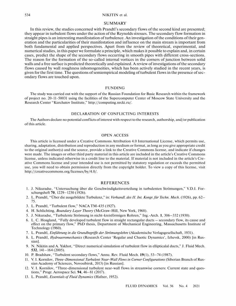
534 NIKITIN et al.
SUMMARYIn this review, the studies concerned with Prandtl’s secondary f lows of the second kind are presented;
they appear in turbulent f lows under the action of the Reynolds stresses. The secondary f low formation instraight pipes is an interesting manifestation of turbulence. An investigation of the conditions of their gen-eration and the particularities of their manifestation and influence on the main stream is important fromboth fundamental and applied perspectives. Apart from the review of theoretical, experimental, andnumerical studies, in this paper we formulate a principle, which makes it possible to explain and, in certaincases, predict the shape of the secondary f lows occurring in smooth pipes with different cross-sections.The reason for the formation of the so-called internal vortices in the corners of junction between solidwalls and a free surface is predicted theoretically and explained. A review of investigations of the secondaryflows caused by wall roughness inhomogeneities, which has been actively studied in the recent years, isgiven for the first time. The questions of semiempirical modeling of turbulent f lows in the presence of sec-ondary f lows are touched upon.
FUNDINGThe study was carried out with the support of the Russian Foundation for Basic Research within the framework
of project no. 20-11-50031 using the facilities of the Supercomputer Center of Moscow State University and theResearch Center “Kurchatov Institute,” http://computing.nrcki.ru/.
DECLARATION OF CONFLICTING INTERESTSThe Authors declare no potential conflicts of interest with respect to the research, authorship, and/or publication
of this article.
OPEN ACCESSThis article is licensed under a Creative Commons Attribution 4.0 International License, which permits use,
sharing, adaptation, distribution and reproduction in any medium or format, as long as you give appropriate creditto the original author(s) and the source, provide a link to the Creative Commons license, and indicate if changeswere made. The images or other third party material in this article are included in the article's Creative Commonslicense, unless indicated otherwise in a credit line to the material. If material is not included in the article's Cre-ative Commons license and your intended use is not permitted by statutory regulation or exceeds the permitteduse, you will need to obtain permission directly from the copyright holder. To view a copy of this license, visithttp://creativecommons.org/licenses/by/4.0/.
REFERENCES1. J. Nikuradse, “Untersuchung über die Geschwindigkeitsverteilung in turbulenten Strömungen,” V.D.I. For-
schungsheft 70, 1229–1230 (1926).2. L. Prandtl, “Über die ausgebildete Turbulenz,” in: Verhandl. des II. Int. Kongr. für Techn. Mech. (1926), pp. 62–
75.3. L. Prandtl, “Turbulent f low,” NACA TM-435 (1927).4. H. Schlichting, Boundary Layer Theory (McGraw-Hill, New York, 1968).5. J. Nikuradse, “Turbulente Strömung in nicht-kreisförmigen Rohren,” Ing.-Arch. 1, 306–332 (1930).6. L. C. Hoagland, “Fully developed turbulent f low in straight rectangular ducts – secondary f low, its cause and
effect on the primary f low,” PhD thesis, Department of Mechanical Engineering, Massachusetts Institute ofTechnology (1960).
7. L. Prandtl, Einführung in die Grundbegriffe der Strömungslehre (Akademische Verlagsgesellschaft, 1931).8. L. Prandtl, Hydroaeromechanics (Research Center ‘Regular and Chaotic Dynamics’, Izhevsk, 2000) [in Rus-
sian].9. N. Nikitin and A. Yakhot, “Direct numerical simulation of turbulent f low in ellipticalal ducts,” J. Fluid Mech.
532, 141–164 (2005).10. P. Bradshaw, “Turbulent secondary f lows,” Annu. Rev. Fluid Mech. 19(1), 53–74 (1987).11. V. I. Kornilov, Three-Dimensional Turbulent Near-Wall Flows in Corner Configurations (Siberian Branch of Rus-
sian Academy of Sciences, Novosibirsk, 2013) [in Russian].12. V. I. Kornilov, “Three-dimensional turbulent near-wall f lows in streamwise corners: Current state and ques-
tions,” Progr. Aerospace Sci. 94, 46–81 (2017).13. L. Prandtl, Essentials of Fluid Dynamics (Hafner, 1952).
FLUID DYNAMICS Vol. 56 No. 4 2021
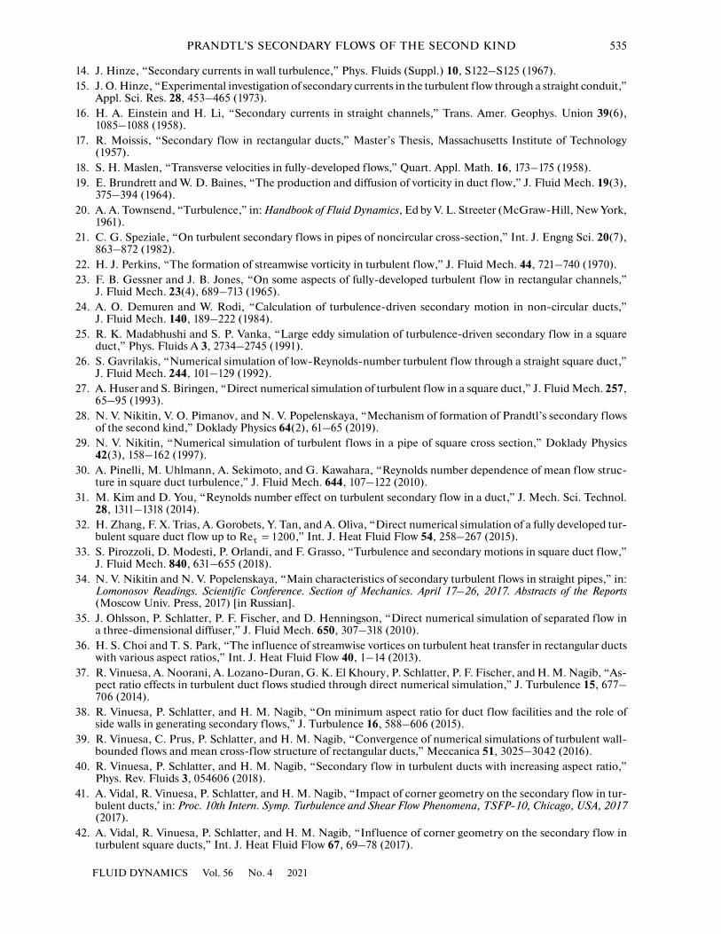
PRANDTL’S SECONDARY FLOWS OF THE SECOND KIND 535
14. J. Hinze, “Secondary currents in wall turbulence,” Phys. Fluids (Suppl.) 10, S122–S125 (1967).15. J. O. Hinze, “Experimental investigation of secondary currents in the turbulent f low through a straight conduit,”
Appl. Sci. Res. 28, 453–465 (1973).16. H. A. Einstein and H. Li, “Secondary currents in straight channels,” Trans. Amer. Geophys. Union 39(6),
1085–1088 (1958).17. R. Moissis, “Secondary f low in rectangular ducts,” Master’s Thesis, Massachusetts Institute of Technology
(1957).18. S. H. Maslen, “Transverse velocities in fully-developed f lows,” Quart. Appl. Math. 16, 173–175 (1958).19. E. Brundrett and W. D. Baines, “The production and diffusion of vorticity in duct f low,” J. Fluid Mech. 19(3),
375–394 (1964).20. A. A. Townsend, “Turbulence,” in: Handbook of Fluid Dynamics, Ed by V. L. Streeter (McGraw-Hill, New York,
1961).21. C. G. Speziale, “On turbulent secondary f lows in pipes of noncircular cross-section,” Int. J. Engng Sci. 20(7),
863–872 (1982).22. H. J. Perkins, “The formation of streamwise vorticity in turbulent f low,” J. Fluid Mech. 44, 721–740 (1970).23. F. B. Gessner and J. B. Jones, “On some aspects of fully-developed turbulent f low in rectangular channels,”
J. Fluid Mech. 23(4), 689–713 (1965).24. A. O. Demuren and W. Rodi, “Calculation of turbulence-driven secondary motion in non-circular ducts,”
J. Fluid Mech. 140, 189–222 (1984).25. R. K. Madabhushi and S. P. Vanka, “Large eddy simulation of turbulence-driven secondary f low in a square
duct,” Phys. Fluids A 3, 2734–2745 (1991).26. S. Gavrilakis, “Numerical simulation of low-Reynolds-number turbulent f low through a straight square duct,”
J. Fluid Mech. 244, 101–129 (1992).27. A. Huser and S. Biringen, “Direct numerical simulation of turbulent f low in a square duct,” J. Fluid Mech. 257,
65–95 (1993).28. N. V. Nikitin, V. O. Pimanov, and N. V. Popelenskaya, “Mechanism of formation of Prandtl’s secondary f lows
of the second kind,” Doklady Physics 64(2), 61–65 (2019).29. N. V. Nikitin, “Numerical simulation of turbulent f lows in a pipe of square cross section,” Doklady Physics
42(3), 158–162 (1997).30. A. Pinelli, M. Uhlmann, A. Sekimoto, and G. Kawahara, “Reynolds number dependence of mean flow struc-
ture in square duct turbulence,” J. Fluid Mech. 644, 107–122 (2010).31. M. Kim and D. You, “Reynolds number effect on turbulent secondary f low in a duct,” J. Mech. Sci. Technol.
28, 1311–1318 (2014).32. H. Zhang, F. X. Trias, A. Gorobets, Y. Tan, and A. Oliva, “Direct numerical simulation of a fully developed tur-
bulent square duct f low up to ,” Int. J. Heat Fluid Flow 54, 258–267 (2015).33. S. Pirozzoli, D. Modesti, P. Orlandi, and F. Grasso, “Turbulence and secondary motions in square duct f low,”
J. Fluid Mech. 840, 631–655 (2018).34. N. V. Nikitin and N. V. Popelenskaya, “Main characteristics of secondary turbulent f lows in straight pipes,” in:
Lomonosov Readings. Scientific Conference. Section of Mechanics. April 17–26, 2017. Abstracts of the Reports(Moscow Univ. Press, 2017) [in Russian].
35. J. Ohlsson, P. Schlatter, P. F. Fischer, and D. Henningson, “Direct numerical simulation of separated f low ina three-dimensional diffuser,” J. Fluid Mech. 650, 307–318 (2010).
36. H. S. Choi and T. S. Park, “The influence of streamwise vortices on turbulent heat transfer in rectangular ductswith various aspect ratios,” Int. J. Heat Fluid Flow 40, 1–14 (2013).
37. R. Vinuesa, A. Noorani, A. Lozano-Duran, G. K. El Khoury, P. Schlatter, P. F. Fischer, and H. M. Nagib, “As-pect ratio effects in turbulent duct f lows studied through direct numerical simulation,” J. Turbulence 15, 677–706 (2014).
38. R. Vinuesa, P. Schlatter, and H. M. Nagib, “On minimum aspect ratio for duct f low facilities and the role ofside walls in generating secondary f lows,” J. Turbulence 16, 588–606 (2015).
39. R. Vinuesa, C. Prus, P. Schlatter, and H. M. Nagib, “Convergence of numerical simulations of turbulent wall-bounded flows and mean cross-flow structure of rectangular ducts,” Meccanica 51, 3025–3042 (2016).
40. R. Vinuesa, P. Schlatter, and H. M. Nagib, “Secondary f low in turbulent ducts with increasing aspect ratio,”Phys. Rev. Fluids 3, 054606 (2018).
41. A. Vidal, R. Vinuesa, P. Schlatter, and H. M. Nagib, “Impact of corner geometry on the secondary f low in tur-bulent ducts,’ in: Proc. 10th Intern. Symp. Turbulence and Shear Flow Phenomena, TSFP-10, Chicago, USA, 2017(2017).
42. A. Vidal, R. Vinuesa, P. Schlatter, and H. M. Nagib, “Influence of corner geometry on the secondary f low inturbulent square ducts,” Int. J. Heat Fluid Flow 67, 69–78 (2017).
τ =Re 1200
FLUID DYNAMICS Vol. 56 No. 4 2021
536 NIKITIN et al.
43. A. Vidal, R. Vinuesa, P. Schlatter, and H. M. Nagib, “Turbulent rectangular ducts with minimum secondaryflow,” Int. J. Heat Fluid Flow 72, 317–328 (2018).
44. J. Kim, D. Kim, and H. Choi, “An immersed-boundary finite-volume method for simulations of f low in com-plex geometries,” J. Comput. Phys. 171, 132–150 (2001).
45. T. V. Voronova and N. V. Nikitin, “Direct numerical simulation of the turbulent f low in an ellipticalal pipe,”Comput. Math. Math. Phys. 46(8), 1378–1386 (2006).
46. T. V. Voronova and N. V. Nikitin, “Results of direct numerical simulation of the turbulent f low in a pipe of el-lipticalal cross-section,” Fluid Dynamics 42(2), 201–211 (2007).
47. N. Nikitin, “Finite-difference method for incompressible Navier–Stokes equations in arbitrary orthogonal cur-vilinear coordinates,” J. Comput. Phys. 217, 759–781 (2006).
48. S. C. Kacker, “Some aspects of fully developed turbulent f low in non-circular ducts,” J. Fluid Mech. 57, 583–602 (1973).
49. J. M. Nouri, H. Umur, and J. H. Whitelaw, “Flow of Newtonian and non-Newtonian fluids in concentric andeccentric annuli,” J. Fluid Mech. 253, 617–641 (1993).
50. N. V. Nikitin, “ Direct numerical simulation of turbulent f lows in eccentric pipes,” Comput. Math. Math. Phys.46(3), 489–504 (2006).
51. N. Nikitin, H. Wang, and S. Chernyshenko, “Turbulent f low and heat transfer in eccentric annulus,” J. FluidMech. 638, 95–116 (2009).
52. N. Kanaris, X. Albets-Chico, and S. C. Kassinos, “Numerical simulations of turbulent f low in an eccentric an-nulus of unit eccentricity,” in: 9th Intern. Symp. on Turbulence and Shear Flow Phenomena, TSFP 2015. vol. 3,TSFP-9. (2015).
53. N. R. Panchapakesan and P. N. Joubert, “Turbulent boundary layer development along a streamwise edge(Chine) – mean flow,” in: 13th Australasian Fluid Mechanics Conference, Monash. (1998), pp. 373–376.
54. N. R. Panchapakesan and P. N. Joubert, “Turbulence measurements in the boundary layer over a streamwiseedge (Chine),” in: Turbulence and Shear Flow Phenomena, Santa Barbara (1999).
55. K. A. M. Moinuddin, P. N. Joubert, and M. S. Chong, “Experimental investigation of turbulence-driven sec-ondary motion over a streamwise external corner,” J. Fluid Mech. 511, 1–23 (2004).
56. H. Xu and A. Pollard, “Large eddy simulation of turbulent f low in a square annular duct,” Phys. Fluids 13(11),3321–3337 (2001).
57. H. Xu, “Direct numerical simulation of turbulence in a square annular duct,” J. Fluid Mech. 621, 23–57 (2009).58. N. V. Nikitin and N. V. Popelenskaya, “Turbulent f low along an external corner,” in: Lomonosov Readings. Sci-
entific Conference. Section of Mechanics. October 2020. Abstracts of the Reports (Moscow Univ. Press, 2020) [inRussian].
59. A. Tominaga, I. Nezu, K. Ezaki, and H. Nakagawa, “Three-dimensional turbulent structure in straight open-channel f lows,” J. Hydraul. Res. 27, 149–173 (1989).
60. I. Nezu and H. Nakagawa, Turbulence in Open-Channel Flows (Balkema, Rotterdam, 1993).61. Y. Pan and S. Banerjee, “Numerical investigation of free-surface turbulence in open-channel f lows,” Phys. Flu-
ids 7, 1649–1664 (1995).62. I. Albayrak and U. Lemmin, “Secondary currents and corresponding surface velocity patterns in a turbulent
open-channel f low over a rough bed,” J. Hydraul. Eng. 137(11), 1318–1334 (2011).63. S.-Q. Yang, S. K. Tan, and X.-K. Wang, “Mechanism of secondary currents in open channel f lows,” J. Geo-
phys. Res. 117, F04014 (2012).64. T. Stoesser, R. McSherry, and B. Fraga, “Secondary currents and turbulence over a non-uniformly roughened
open-channel bed,” Water 7(9), 4896–4913 (2015).65. I. Nezu. and W. Rodi, “Experimental study on secondary currents in open channels f low,” in: Proc. 21st Con-
gress of IAHR. 2. Melbourne. Australia (1985), pp. 19–23.66. L. M. Grega, T. Wey, R. I. Leighton, and J. C. Neves, “Turbulent mixed-boundary f low in a corner formed by
a solid wall and a free-surface,” J. Fluid Mech. 294, 17–46 (1995).67. R. Broglia, A. Pascarelli, and U. Piomelli, “Large-eddy simulations of ducts with a free surface,” J. Fluid Mech.
484, 223–253 (2003).68. W. Anderson, J Barros., K. Christensen, and A. Awasthi, “Numerical and experimental study of mechanisms
responsible for turbulent secondary f lows in boundary layer f lows over spanwise heterogeneous roughness,”J. Fluid Mech. 768, 316–347 (2015).
69. O. Marin, R. Vinuesa, A. V. Obabko, and P. Schlatter, “Characterization of the secondary f low in hexagonalducts,” Phys. Fluids 28, 125101 (2016).
70. C. Vanderwel, A. Stroh, J. Kriegseis, B. Frohnapfel, and B. Ganapathisubramani, “The instantaneous structureof secondary f lows in turbulent boundary layers,” J. Fluid Mech. 862, 845–870 (2019).
71. K. Nagata, J. C. R. Hunt, Y. Sakai, and H. Wong, “Distorted turbulence and secondary f low near right-angledplates,” J. Fluid Mech. 668, 446–479 (2011).
FLUID DYNAMICS Vol. 56 No. 4 2021
PRANDTL’S SECONDARY FLOWS OF THE SECOND KIND 537
72. E. A. Eichelbrenner and J. H. Preston, “On the role of secondary f low in turbulent boundary layers in corners(and salients),” J. Mécanique 10, 91–112 (1971).
73. F. B. Gessner, “The origin of secondary f low in turbulent f low along a corner,” J. Fluid Mech. 58, 1–25 (1973).74. Dai Yi-Jun and Xu Chun-Xiao, “Wall pressure and secondary-flow origination in a square duct,” Phys. Fluids
31, 085104 (2019).75. N. Nikitin, “Turbulent secondary f lows in channels with no-slip and shear-free boundaries,” J. Fluid Mech.
917, A24 (2021).76. D. E. Pivovarov, N. V. Popelenskaya, and N. V. Nikitin, “Direct numerical simulation of turbulent f low over an
external corner,” in: Abstracts of the Reports Presented to XXIV International Conference ‘Nonlinear Problems ofHydrodynamic Stability and Turbulence’, Ed by N. V. Nikitin and N. V. Popelenskaya (Moscow Univ. Press,2020) [in Russian].
77. J Bons., R. Taylor, S. McClain, R. Rivir, “The many faces of turbine surface roughness,” in: ASME Turbo Expo2001: Power for Land, Sea, and Air (2001), pp. V003T01A042–V003T01A042.
78. R. Mejia-Alvarez and K. T. Christensen, “Wall-parallel stereo particle image velocimetry measurements in theroughness sublayer of turbulent f low over-lying highly irregular roughness,” Phys. Fluids 25(11), 115109 (2013).
79. J. M. Barros and K. T. Christensen, “Observations of turbulent secondary f lows in a rough-wall boundary lay-er,” J. Fluid Mech. 748, R1 (2014).
80. Z.-Q. Wang and N.-S. Cheng, “Time-mean structure of secondary f lows in open channel with longitudinalbedforms,” Adv. Water Resources 29(11), 1634–1649 (2006).
81. I. Castro, J. Kim, A. Stroh, and H. Lim, “Channel f low with large longitudinal ribs,” J. Fluid Mech. 915, A92(2021).
82. D. Chung, J. P. Monty, and N. Hutchins, “Similarity and structure of wall turbulence with lateral wall shearstress variations,” J. Fluid Mech. 847, 591–613 (2018).
83. D. Willingham, W. Anderson, K. T. Christensen, and J. M. Barros, “Turbulent boundary layer f low over trans-verse aerodynamic roughness transitions: Induced mixing and flow characterization,” Phys. Fluids 26(2),025111 (2014).
84. Y. Zheng and W. Anderson, “Flow-roughness heterogeneity: critical obliquity and salient parameters,” J. FluidMech. 913, A12 (2021).
85. S. Türk, G. Daschiel, A. Stroh, Y. Hasegawa, and B. Frohnapfel, “Turbulent f low over superhydrophobic sur-faces with streamwise grooves,” J. Fluid Mech. 747, 186–217 (2014).
86. D. D. Wangsawijaya, R. Baidya, D. Chung, I. Marusic, and N. Hutchins, “The effect of spanwise wavelengthof surface heterogeneity on turbulent secondary f lows,” J. Fluid Mech. 894, A7 (2020).
87. A. Stroh, K. Schäfer, P. Forooghi, and B. Frohnapfel, “Secondary f low and heat transfer in turbulent f low overstreamwise ridges,” Int. J. Heat Fluid Flow 81, 108518 (2020).
88. D. B. Goldstein and T.-C. Tuan, “Secondary f low induced by riblets,” J. Fluid Mech. 363, 115–151 (1998).89. C. Vanderwel and B. Ganapathisubramani, “Effects of spanwise spacing on large-scale secondary f lows in
rough-wall turbulent boundary layers,” J. Fluid Mech. 774, 1–12 (2015).90. T. Medjnoun, C. Vanderwel, and B. Ganapathisubramani, “Characteristics of turbulent boundary layers over
smooth surfaces with spanwise heterogeneities,” J. Fluid Mech. 838, 516–543 (2018).91. A. Zampiron, S. Cameron, and V. Nikora, “Secondary currents and very-large-scale motions in open-channel
flow over streamwise ridges,” J. Fluid Mech. 887, A17 (2020).92. H. Hwang and J. Lee, “Secondary f lows in turbulent boundary layers over longitudinal surface roughness,”
Phys. Rev. Fluids 3, 014608 (2018).93. J. Yang and W. Anderson, “Numerical study of turbulent channel f low over surfaces with variable spanwise het-
erogeneities: Topographically-driven secondary f lows affect external-layer similarity of turbulent length scales,”Flow, Turbulence, Combustion 100(1), 1–17 (2018).
94. A. Stroh, K. Schäfer, B. Frohnapfel, and P. Forooghi, “Rearrangement of secondary f low over spanwise het-erogeneous roughness,” J. Fluid Mech. 885, R5 (2020).
95. S. Pope, Turbulent Flows (Cambridge, 2001).96. M. Leschziner and D. Drikakis, “Turbulence modelling and turbulent-flow computation in aeronautics,” Aero-
naut. J. 106, 349–384 (2002).97. R. Pecnik and G. Iaccarino, “Predictions of turbulent secondary f lows using the – model,” in: 38th Fluid
Dynamics Conference and Exhibit (2008), p. 3852.98. P. Spalart and S. Allmaras, “A one-equation turbulence model for aerodynamic f lows,” in: 30th Aerospace Sci-
ences Meeting and Exhibit (1992), p. 439.99. W. Jones and B. Launder, “The prediction of laminarization with a two-equation model of turbulence,” Int. J.
Heat Mass Transfer 15(2), 301–314 (1972).100. D. Wilcox, Turbulence Modeling for CFD, Vol. 2 (DCW Industries, La Canada 1993).
v2 f
FLUID DYNAMICS Vol. 56 No. 4 2021
538 NIKITIN et al.
101. F. Menter, “Two-equation eddy-viscosity turbulence models for engineering applications,” AIAA J. 32(8),1598–1605 (1994).
102. G. Alfonsi, “Reynolds-averaged Navier–Stokes equations for turbulence modeling,” Appl. Mech. Rev. 62(4),040802 (2009).
103. P. Durbin, “Near-wall turbulence closure modeling without ‘damping functions’,” Theor. Comput. Fluid Dyn.3(1), 1–13 (1991).
104. J. Rotta, “Statistische Theorie nichthomogener Turbulenz,” Zeitschrift für Physik 129(6), 547–572 (1951).105. D. Naot, A. Savit, and M. Wolfshtin, “Numerical calculation of Reynolds stresses in a square duct with sec-
ondary f low,” Wärme- und Stoffübertragung 7(3), 151–161 (1974).106. G. Reece, “Development and application of a generalized Reynolds-stress model of turbulence,” PhD Thesis,
University of London (1977).107. H. Leutheusser, “Turbulent f low in rectangular ducts,” J. Hydraul. Eng. 89(3), 1–19 (1963).108. B. Launder and W. Ying, “Prediction of f low and heat transfer in ducts of square cross-section,” Proc. Inst. Me-
chanical Engineers 187(1), 455–461 (1973).109. C. Speziale, S. Sarkar, and T. Gatski, “Modelling the pressure-strain correlation of turbulence: an invariant dy-
namical systems approach,” J. Fluid Mech. 227, 245–272 (1991).110. B. Launder, G. Reece, and W. Rodi, “Progress in the development of a Reynolds-stress turbulence closure,”
J. Fluid Mech. 68(3), 537–566 (1975).111. N. de Cacqueray, D. Hargreaves, and H. Morvan, “A computational study of shear stress in smooth rectangular
channels,” J. Hydraul. Res. 47(1), 50–57 (2009).112. H. Kang and S. Choi, “Reynolds stress modelling of rectangular open channel f low,” Intern. J. Numer. Meth-
ods Fluids 51(11), 1319–1334 (2006).113. K. Ansari, H. P. Morvan, and D. M. Hargreaves, “Numerical investigation into secondary currents and wall
shear in trapezoidal channels,” J. Hydraul. Eng. 137(4), 432–440 (2011).114. H. Jing, Y. Guo, C. Li, and J. Zhang, “Three-dimensional numerical simulation of compound meandering
open channel f low by the Reynolds stress model,” Intern. J. Numer. Methods Fluids. 59(8), 927–943 (2009).115. S. Choi and H. Kang, “Characteristics of mean flow and turbulence statistics of depth-limited f lows with sub-
merged vegetation in a rectangular open channel,” J. Hydraul. Res. 54(5), 527–540 (2016).116. K. Hanjalic and B. Launder, “A Reynolds stress model of turbulence and its application to thin shear f lows,”
J. Fluid Mech. 52(4), 609–638 (1972).117. S. Kacker, “Discussion of ‘prediction of f low and heat transfer in ducts of square cross-section’,” Proc. Inst.
Mechanical Engineers 187, D147–D148 (1973).118. A. Nakayama, W. Chow, and D. Sharma, “Calculation of fully developed turbulent f lows in ducts of arbitrary
cross-section,” J. Fluid Mech. 128, 199–217 (1983).119. D. Tatchell, “Convection processes in confined three-dimensional boundary layers,” PhD Thesis. Imperial
College London (1975).120. A. Gosman and C. Rapley, “Fully-developed f low in passages of arbitrary cross-section,” Recent Advances in
Numerical Methods in Fluids 1, 335–399 (1980).121. C. Rapley, “The simulation of secondary f low effects in turbulent noncircular passage f lows,” Intern. J. Numer.
Methods Fluids 2(4), 331–347 (1982).122. D. Naot and W. Rodi, “Calculation of secondary currents in channel f low,” J. Hydraul. Eng. 108(8), 948–968
(1982).123. C. Speziale, “On nonlinear and models of turbulence,” J. Fluid Mech. 178, 459–475 (1987).124. B. Younis and O. Abdellatif, “Modeling sediment transport in rectangular ducts with a two-equation model of
turbulence,” in: Sediment Transport Modeling (ASCE, 1989), pp. 197–202.125. N. Hur, S. Thangam, and C. Speziale, “Numerical study of turbulent secondary f lows in curved ducts,” J. Fluid
Eng. 112, 205–211 (1990).126. D. Cokljat, “Turbulence models for non-circular ducts and channels,” PhD Thesis. City University London
(1993).127. D. Cokljat and B. Younis, “Second-order closure study of open-channel f lows,” J. Hydraul. Eng. 121(2), 94–
107 (1995).128. M. Tajnesaie, E. J. Nodoushan, R. Barati, and M. A. Moghadam, “Performance comparison of four turbulence
models for modeling of secondary f low cells in simple trapezoidal channels,” J. Hydraul. Eng. 26(2), 187–197(2020).
Translated by M. Lebedev
−k l − εk
FLUID DYNAMICS Vol. 56 No. 4 2021