Pre-aggregation functions: construction and an application

1

Pre-aggregation functions: construction and anapplication

Giancarlo Lucca, Jose Antonio Sanz, Gracaliz Pereira Dimuro, Benjamın Bedregal, Radko Mesiar, AnnaKolesarova, Humberto Bustince,IEEE Senior Member

Abstract—In this work we introduce the notion of pre-aggregation function. Such a function satisfies the same boundaryconditions as an aggregation function, but, instead of requiringmonotonicity, only monotonicity along some fixed direction (di-rectional monotonicity) is required. We present some examplesof such functions. We propose three different methods to buildpre-aggregation functions. We experimentally show that in fuzzyrule-based classification systems, when we use one of thesemethods, namely, the one based on the use of the Choquetintegral replacing the product by other aggregation functions,if we consider the minimum or the Hamacher product t-normsfor such construction, we improve the results obtained whenapplying the fuzzy reasoning methods obtained using two classicalaveraging operators like the maximum and the Choquet integral.

Index Terms—Aggregation functions, directional monotonicity,fuzzy measures, Choquet integral, fuzzy rule-based classificationsystems, fuzzy reasoning method

I. I NTRODUCTION

Aggregation functions [1], [2] are crucial tools nowadays todeal with many computation problems [3], [4], [5], [6], [7].The key property for defining them, apart from the boundaryconditions, is monotonicity and, more specifically, monotoneincreasingness. However, some other statistical tools, such asthe mode, are not included in this family, although they areuseful, since, even if they are properly defined as functions,monotonicity is violated.

The problem of relaxing the definition of monotonicity hasrecently attracted a lot of interest. In [8], Wilkin and Beliakovproposed the notion of weak monotonicity in order to extendthe usual monotonicity property. In this case, monotonicity is

This work was supported in part by the Spanish Ministry of Sci-ence and Technology under projects TIN2008-06681-C06-01,TIN2010-15055, TIN2013-40765-P, TIN2011-29520, by the Brazilian funding agencyCNPQ under Processes 481283/2013-7, 306970/2013-9, 232827/2014-1 and307681/2012-2, and by grants VEGA 1/0419/13 and VEGA 1/0420/15.

G. Lucca and G. Pereira Dimuro are with PPGCOMP, Centro de CienciasComputacionais, Universidade Federal do Rio Grande, Rio Grande, Brazil,e-mail: [email protected]

J. Sanz and H. Bustince are with the Departamento ofAutomatica y Computacion and with the Institute of Smart Cities,Universidad Publica de Navarra, Navarra, 31006 Spain e-mails:{joseantonio.sanz,bustince}@unavarra.es.

B. Bedregal is with Departamento de Informatica e Matematica Aplicada,Universidade Federal do Rio Grande do Norte, Natal, Brazil,e-mail: [email protected].

R. Mesiar is with the Slovak University of Technology, Radlinskeho 11,810 05 Bratislava, Slovakia and with the Institute of Information Theory andAutomation, Academy of Sciences of the Czech Republic, 18208 Prague,Czech Republic

A. Kolesarova is with the Institute of Information Engineering, Automa-tion and Mathematics, Slovak University of Technology, 812 37 Bratislava,Slovakia.

required only along the direction of the first quadrant diagonal.This concept of weak monotonicity has been further extendedby Bustince et al. [9] by introducing the notion of directionalmonotonicity, which allows monotonicity along (some) fixedray. In particular, directionally monotone functions encom-pass weak monotone functions, as well as the mode and anyaggregation function.

In particular, in this paper we consider the following objec-tives:

1) To introduce the concept of pre-aggregation functions.2) To study the first properties of these new functions.3) To introduce three different methods for building pre-

aggregation functions.4) To show an application where the introduction of the

new concept of pre-aggregation function is justified.To achieve these goals we use the notion of directional

monotonicity. Moreover, for one of the construction methodsthat we propose, in the definition of the Choquet integral wereplace the product by the minimum or the Hamacher productt-norm, and, in this way, we obtain pre-aggregation functionsthat are not aggregation functions. We show that using thesenew functions in a Fuzzy Rule-based Classification System(FRBCS), and, in particular, in the Fuzzy Reasoning Method(FRM) of FARC-HD [10], which is currently one of the mostaccurate FRBCSs, the obtained results are better than bothapplying the classical Choquet integral and the well-knownFRM of the winning rule.

This paper is organized as follows. In Section II, wepresent some related preliminary concepts that are necessary tounderstand the paper. In Section III we introduce the notionofpre-aggregation function and discuss some properties. Threemethods of construction of pre-aggregation functions aredescribed in Section IV. The generalization of the FRM usingpre-aggregation functions is described in detail in Section V.The experimental framework and the analysis of the obtainedresults when considering some of our pre-aggregation func-tions are reported in Section VI. In Section VII we draw themain conclusions and the detailed results of the experimentsare available in the Appendix.

II. PRELIMINARIES

A. Aggregation functions

An important class of operators that are used in this paperare theaggregation functions[1], [11]:

Definition 2.1: A function A : [0, 1]n → [0, 1] is said tobe ann-ary aggregation function if the following conditionshold:

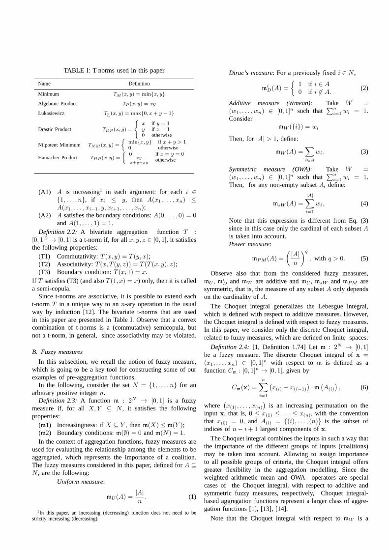
TABLE I: T-norms used in this paper

Name Definition

Minimum TM (x, y) = min{x, y}

Algebraic Product TP (x, y) = xy

Łukasiewicz TŁ(x, y) = max{0, x+ y − 1}

Drastic Product TDP (x, y) =

x if y = 1y if x = 10 otherwise

Nilpotent Minimum TNM (x, y) =

{

min{x, y} if x+ y > 10 otherwise

Hamacher Product THP (x, y) =

{

0 if x = y = 0xy

x+y−xyotherwise

(A1) A is increasing1 in each argument: for eachi ∈{1, . . . , n}, if xi ≤ y, then A(x1, . . . , xn) ≤A(x1, . . . , xi−1, y, xi+1, . . . , xn);

(A2) A satisfies the boundary conditions:A(0, . . . , 0) = 0andA(1, . . . , 1) = 1.

Definition 2.2: A bivariate aggregation functionT :[0, 1]2 → [0, 1] is a t-norm if, for allx, y, z ∈ [0, 1], it satisfiesthe following properties:

(T1) Commutativity:T (x, y) = T (y, x);(T2) Associativity:T (x, T (y, z)) = T (T (x, y), z);(T3) Boundary condition:T (x, 1) = x.

If T satisfies (T3) (and alsoT (1, x) = x) only, then it is calleda semi-copula.

Since t-norms are associative, it is possible to extend eacht-norm T in a unique way to ann-ary operation in the usualway by induction [12]. The bivariate t-norms that are usedin this paper are presented in Table I. Observe that a convexcombination of t-norms is a (commutative) semicopula, butnot a t-norm, in general, since associativity may be violated.

B. Fuzzy measures

In this subsection, we recall the notion of fuzzy measure,which is going to be a key tool for constructing some of ourexamples of pre-aggregation functions.

In the following, consider the setN = {1, . . . , n} for anarbitrary positive integern.

Definition 2.3: A function m : 2N → [0, 1] is a fuzzymeasure if, for allX,Y ⊆ N , it satisfies the followingproperties:

(m1) Increasingness: ifX ⊆ Y , thenm(X) ≤ m(Y );(m2) Boundary conditions:m(∅) = 0 andm(N) = 1.In the context of aggregation functions, fuzzy measures are

used for evaluating the relationship among the elements to beaggregated, which represents the importance of a coalition.The fuzzy measures considered in this paper, defined forA ⊆N , are the following:

Uniform measure:

mU (A) =|A|

n. (1)

1In this paper, an increasing (decreasing) function does notneed to bestrictly increasing (decreasing).

Dirac’s measure: For a previously fixedi ∈ N ,

miD(A) =

{

1 if i ∈ A0 if i 6∈ A.

(2)

Additive measure (Wmean): Take W =(w1, . . . , wn) ∈ [0, 1]n such that

∑ni=1 wi = 1.

ConsidermW ({i}) = wi

Then, for |A| > 1, define:

mW (A) =∑

i∈A

wi. (3)

Symmetric measure (OWA): Take W =(w1, . . . , wn) ∈ [0, 1]n such that

∑ni=1 wi = 1.

Then, for any non-empty subsetA, define:

msW (A) =

|A|∑

i=1

wi. (4)

Note that this expression is different from Eq. (3)since in this case only the cardinal of each subsetAis taken into account.Power measure:

mPM (A) =

(

|A|

n

)q

, with q > 0. (5)

Observe also that from the considered fuzzy measures,mU , mi

D andmW are additive andmU , msW andmPM aresymmetric, that is, the measure of any subsetA only dependson the cardinality ofA.

The Choquet integral generalizes the Lebesgue integral,which is defined with respect to additive measures. However,the Choquet integral is defined with respect to fuzzy measures.In this paper, we consider only the discrete Choquet integral,related to fuzzy measures, which are defined on finite spaces:

Definition 2.4: [1, Definition 1.74] Letm : 2N → [0, 1]be a fuzzy measure. The discrete Choquet integral ofx =(x1, . . . , xn) ∈ [0, 1]n with respect tom is defined as afunctionCm : [0, 1]n → [0, 1], given by

Cm(x) =

n∑

i=1

(

x(i) − x(i−1)

)

·m(

A(i)

)

, (6)

where(

x(1), . . . , x(n)

)

is an increasing permutation on theinput x, that is,0 ≤ x(1) ≤ . . . ≤ x(n), with the conventionthat x(0) = 0, and A(i) = {(i), . . . , (n)} is the subset ofindices ofn− i+ 1 largest components ofx.

The Choquet integral combines the inputs in such a way thatthe importance of the different groups of inputs (coalitions)may be taken into account. Allowing to assign importanceto all possible groups of criteria, the Choquet integral offersgreater flexibility in the aggregation modelling. Since theweighted arithmetic mean and OWA operators are specialcases of the Choquet integral, with respect to additive andsymmetric fuzzy measures, respectively, Choquet integral-based aggregation functions represent a larger class of aggre-gation functions [1], [13], [14].

Note that the Choquet integral with respect tomW is a

weighted arithmetic mean, and with respect tomsW is an OWAoperator2. These facts explain the acronyms we have chosenin the present work for these measures.

C. Directional monotonicity

This subsection is devoted to recalling the basic concept forour definition of pre-aggregation function, that of directionalmonotonicity [9].

Definition 2.5: Let ~r = (r1, . . . , rn) be a real n-dimensional vector,~r 6= ~0. A function F : [0, 1]n → [0, 1]is ~r-increasing if for all points(x1, . . . , xn) ∈ [0, 1]n and forall c > 0 such that(x1 + cr1, . . . , xn + crn) ∈ [0, 1]n it holds

F (x1 + cr1, . . . , xn + crn) ≥ F (x1, . . . , xn) .

That is, an~r-increasing function is a function which isincreasing along the ray (direction) determined by the vector~r. For this reason, we say thatF is directionally monotone,or, more specifically, directionally increasing. Note thateveryincreasing function (in the usual sense) is, in particular,~r-increasing, for every non-negative real vector~r. However,the class of directionally increasing functions is much widerthan that of aggregation functions. For instance:

• Fuzzy implication functions (see [21]) are(−1, 1)-increasing functions. This implies that many other func-tions, which are widely used in applications and whichcan be obtained from implication functions, are alsodirectionally increasing. This is the case, for instance,of some subsethood measures (see [22]);

• Many functions used for comparison of data are alsodirectionally increasing. In particular, this is the case ofthose based on component-wise comparison by means ofthe Euclidean distance|x − y|, as for restricted equiva-lence functions [23];

• Weakly increasing functions ([8]) are a particular caseof directionally increasing functions, with~r = (1, . . . , 1).

III. PRE-AGGREGATION FUNCTIONS

In this section we introduce the notion of pre-aggregationfunction and discuss some properties and construction meth-ods.

Definition 3.1: A function F : [0, 1]n → [0, 1] is said to bean n-ary pre-aggregation function if the following conditionshold:

(PA1) There exists a real vector~r ∈ [0, 1]n (~r 6= ~0) suchthatF is ~r-increasing.

(PA2) F satisfies the boundary conditions:F (0, . . . , 0) = 0andF (1, . . . , 1) = 1.

Example 3.1:Some examples of pre-aggregation functionsare the following.

(i) Consider the mode,Mod(x1, . . . , xn), defined as thefunction that gives back the value which appears mosttimes in the consideredn-tuple, or the smallest of thevalues that appears most times, in case there is more than

2The OWA operators were first introduced by Yager [15], and several formsand usage of OWA operators have been discussed in the literature [16], [17],[18], [19], [20].

one. Then, the mode is(1, . . . , 1)-increasing, and it is aparticular case of pre-aggregation function which is notan aggregation function.

(ii) F (x, y) = x− (max{0, x− y})2 is, for instance,(0, 1)-increasing, and it is an example of a pre-aggregationfunction which is not an aggregation function.

(iii) Weakly increasing functions satisfying the boundarycon-ditions (PA2) are also pre-aggregation functions whichneed not be aggregation functions.

(iv) Take λ ∈]0, 1[. The weighted Lehmer meanLλ :[0, 1]2 → [0, 1], given by

Lλ(x, y) =λx2 + (1− λ)y2

λx+ (1− λ)y

(with convention0/0 = 0) is (1− λ, λ)-increasing, so itis a pre-aggregation function.

(v) DefineA,B : [0, 1]2 → [0, 1] by

A(x, y) =

{

x(1− x) if y ≤ 3/4 ,

1 otherwise,

and

B(x, y) =

{

y(1− y) if x ≤ 3/4 ,

1 otherwise.

Then bothA andB are pre-aggregation functions whichare not aggregation functions. In fact,A is (0, a)-increasing for anya > 0 but for no other direction~r = (a, b), b > 0, while B is (b, 0)-increasing for anyb > 0 but for no other direction~r = (a, b), a > 0.However, C = (A + B)/2 is not a pre-aggregationfunction, just illustrating the fact that the class of all pre-aggregation functions with a fixed dimensionn is not aconvex class.

If F is a pre-aggregation function with respect to a vector~r we just say thatF is an~r-pre-aggregation function.

Remark 3.1:Note that ifA : [0, 1]n → [0, 1] is an aggre-gation function, thenA is also a pre-aggregation function. Infact, if, for a non-zero vector~r ∈ [0, 1]n we denote byPA~r

the class of all~r-increasing pre-aggregation functions, thenthe class of all pre-aggregation functionsPA is the unionof all these classesPA~r, while the class of all aggregationfunctions is the intersection of all the classesPA~r. The latterintersection is the same as the intersection overPA~ei , where~ei = (0, ..1, ..0), i ∈ {1, . . . , n}, is the vector having 1 asi-thvalue, and all other coordinates are equal to zero.

Note that the reverse of the first claim of Remark 3.1 doesnot hold, as the cases considered in Example 3.1 (i) and (ii)show. Pre-aggregation functions which are not aggregationfunctions will be called proper pre-aggregation functions.However, we can use aggregation functions to obtain direc-tionally increasing functions as follows.

The next results were proved for directionally monotonefunctions in our recent paper [9].

Proposition 3.1:Let A : [0, 1]m → [0, 1] be an aggregationfunction. Let Fi : [0, 1]n → [0, 1] (i ∈ {1, . . . ,m}) be afamily of m ~r-pre-aggregation functions for the same vector~r ∈ [0, 1]n. Then, the functionA(F1, . . . , Fm) : [0, 1]n →

[0, 1], defined as

A(F1, . . . , Fm)(x1, . . . , xn) =

A(F1(x1, . . . , xn), . . . , Fm(x1, . . . , xn))

is also an~r-pre-aggregation function.Proof:

Due to ([9], Proposition 3), only the boundary conditions forthe functions(F1, . . . , Fm) should be guaranteed. However,their validity is obvious.

The following corollary is straightforward.Corollary 3.1: Let F1, F2 : [0, 1]n → [0, 1] be two ~r-pre-

aggregation functions for the same vector~r ∈ [0, 1]n. Then:

(i) F1+F2

2 is also an~r-pre-aggregation function.(ii) F1F2 is also an~r-pre-aggregation function.

Regarding duality, we can state the following.Proposition 3.2:Let F : [0, 1]n → [0, 1] be an ~r-pre-

aggregation function for~r ∈ [0, 1]n. Then, the function

F d(x1, . . . , xn) = 1− F (1− x1, . . . , 1− xn)

is also an~r-pre-aggregation function.Proof:

Obviously,F d(0, . . . , 0) = 0 andF d(1, . . . , 1) = 1. Now,the result follows from ([9], Proposition 3).

The following corollary is now straight.Corollary 3.2: Let F be an ~r- pre-aggregation function.

Then, the functionF+Fd

2 is a self-dual~r-pre-aggregationfunction.

IV. T HREE METHODS OF CONSTRUCTING

PRE-AGGREGATION FUNCTIONS

In this section we introduce and illustrate three methodsof constructing pre-aggregation functions. The first method isbased on the composition of appropriate functions, the secondone is inspired by the construction of the discrete Choquetintegral, and the third of the proposed methods is inspired bythe construction of the discrete Sugeno integral.

A. Construction of pre-aggregation functions by composition

Fix n ∈ N. Let I be a proper subset ofN = {1, . . . , n} andconsider thatI = {i1, . . . , ik} with i1 < . . . < ik. For ann-tuple x = (x1, . . . , xn) ∈ [0, 1]n, its I-projection is ak-tuplexI = (xi1 , . . . , xik), wherek is the cardinality ofI. We willuse I-projectionsxI of points x ∈ [0, 1]n and I-projections~rI of (geometrical) vectors~r ∈ [0, 1]n as well. Finally, fora functionF : [0, 1]n → [0, 1], let D↑(F ) = {~r ∈ [0, 1]n |F is ~r - increasing}. Note that the zero vector is not excludednow.

Proposition 4.1:Let {I1, . . . , Ik} be a partition ofN , k >1. For j ∈ {1, . . . , k}, let nj = |Ij | and consider functionsFj : [0, 1]

nj → [0, 1] such thatFj(1, . . . , 1) = 1. Then, forany aggregation functionG : [0, 1]k → [0, 1], the compositefunctionH : [0, 1]n → [0, 1] defined by

H(x) = G (F1 (xI1) , . . . , Fk (xIk))

is ~r-increasing for any vector~r ∈ [0, 1]n such that~rIj ∈D↑(Fj), j = 1, . . . , k, andH(1) = 1. Moreover, if there is aj0 ∈ {1, . . . , k} such thatFj0 is a pre-aggregation function,and 0 is an annihilator ofG, then the functionH is a pre-aggregation function.

Proof: Clearly, H(1) = G (F1 (1I1) , . . . , Fk (1Ik)) =G(1, . . . , 1) = 1. Moreover, if Fj0(0, . . . , 0) = 0 for somej0 ∈ {1, . . . , k} and0 is an annihilator ofG, then

H(0) = G(

F1 (0I1) , . . . , Fj0

(

0Ij0

)

, . . . , Fk (0Ik))

= G (F1 (0I1) , . . . , 0, . . . , Fk (0Ik)) = 0.

Next, consider a vector~r ∈ [0, 1]n such that~rIj ∈ D↑(Fj)for eachj = 1, . . . , k. Then, for anyc > 0 and x ∈ [0, 1]n

such that alsox+ c~r ∈ [0, 1]n, it holds that

H(x+ c~r) = G (F1 (xI1 + c~rI1) , . . . , Fk (xIk + c~rIk))

≥ G (F1 (xI1) , . . . , Fk (xIk)) = H(x),

where the inequality follows from the increasing mono-tonicity of the aggregation functionG, and the fact thatFj

(

xIj + c~rIj)

≥ Fj

(

xIj

)

, j = 1, . . . , k.Now, suppose thatFj0 is a pre-aggregation function,

i.e., Fj0(0, . . . , 0) = 0 and Fj0 is ~v-increasing for somenon-zero vector~v ∈ [0, 1]nj0 . Due to the above men-tioned facts,H satisfies the boundary conditions and isdirectionally increasing in the direction of a non-zero vec-tor ~r ∈ [0, 1]n such that ~rIj0 = ~v and ~rN\Ij0

=(0, . . . , 0), which proves thatH is a pre-aggregation function.

�

Example 4.1: Let n = 2 and ~v = (v1, v2) ∈ ]0, 1]2.For obtaining a proper pre-aggregation function which is~v-increasing, it is enough to consider the weighted Lehmer meanLλ : [0, 1]

2 → [0, 1] with λ = v2

v1+v2, see Example 3.1(iv),

given by

Lλ(x, y) =v2x

2 + v1y2

v2x+ v1y.

This fact and Proposition 4.1 allow us to construct a pre-aggregation functionH which is directionally increasing inthe direction of any a-priori given vector~0 6= ~r ∈ [0, 1]n.

Consider, for example,n = 4 and~r = (0.5, 0.4, 0.3, 0.7).Let G = TM , I1 = {1, 3}, I2 = {2, 4}, F1 = L3/8, F2 =L7/11. ThenH : [0, 1]4 → [0, 1] given by

H(x1, x2, x3, x4) = min

{

3x21 + 5x2

3

3x1 + 5x3,7x2

2 + 4x24

7x2 + 4x4

}

is an~r-increasing proper pre-aggregation function.

B. Choquet-like construction method of pre-aggregation func-tions

This method is inspired in the way the Choquet integral isbuilt, replacing the product operation in Equation (6) by otheraggregation functions.

Let m : 2N → [0, 1] be a fuzzy measure andM : [0, 1]2 →[0, 1] be a function such thatM(0, x) = 0 for everyx ∈ [0, 1].Taking as basis the Choquet integral, we define the function

CMm

: [0, 1]n → [0, n] by

CMm(x) =

n∑

i=1

M(

x(i) − x(i−1),m(

A(i)

))

, (7)

where N = {1, . . . , n}, (x(1), . . . , x(n)) is an increasingpermutation on the inputx, that is,0 ≤ x(1) ≤ . . . ≤ x(n),with the convention thatx(0) = 0, andA(i) = {(i), . . . , (n)}is the subset of indices ofn− i+ 1 largest components ofx.Note thatCM

mis well defined by (7) even if the permutation

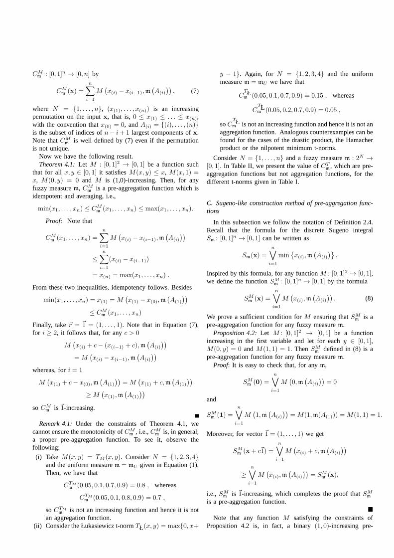
is not unique.Now we have the following result.Theorem 4.1:Let M : [0, 1]2 → [0, 1] be a function such

that for all x, y ∈ [0, 1] it satisfiesM(x, y) ≤ x, M(x, 1) =x, M(0, y) = 0 and M is (1,0)-increasing. Then, for anyfuzzy measurem, CM

mis a pre-aggregation function which is

idempotent and averaging, i.e.,

min(x1, . . . , xn) ≤ CMm(x1, . . . , xn) ≤ max(x1, . . . , xn).

Proof: Note that

CMm(x1, . . . , xn) =

n∑

i=1

M(

x(i) − x(i−1),m(

A(i)

))

≤n∑

i=1

(x(i) − x(i−1))

= x(n) = max(x1, . . . , xn) .

From these two inequalities, idempotency follows. Besides

min(x1, . . . , xn) = x(1) = M(

x(1) − x(0),m(

A(1)

))

≤ CMm(x1, . . . , xn)

Finally, take~r = ~1 = (1, . . . , 1). Note that in Equation (7),for i ≥ 2, it follows that, for anyc > 0

M(

x(i) + c− (x(i−1) + c),m(

A(i)

))

= M(

x(i) − x(i−1),m(

A(i)

))

whereas, fori = 1

M(

x(1) + c− x(0),m(

A(1)

))

= M(

x(1) + c,m(

A(1)

))

≥ M(

x(1),m(

A(1)

))

soCMm

is ~1-increasing.

Remark 4.1:Under the constraints of Theorem 4.1, wecannot ensure the monotonicity ofCM

m, i.e.,CM

mis, in general,

a proper pre-aggregation function. To see it, observe thefollowing:

(i) Take M(x, y) = TM (x, y). ConsiderN = {1, 2, 3, 4}and the uniform measurem = mU given in Equation (1).Then, we have that

CTMm

(0.05, 0.1, 0.7, 0.9) = 0.8 , whereas

CTMm

(0.05, 0.1, 0.8, 0.9) = 0.7 ,

soCTMm

is not an increasing function and hence it is notan aggregation function.

(ii) Consider the Łukasiewicz t-normTŁ(x, y) = max{0, x+

y − 1}. Again, for N = {1, 2, 3, 4} and the uniformmeasurem = mU we have that

CTŁm (0.05, 0.1, 0.7, 0.9) = 0.15 , whereas

CTŁm (0.05, 0.2, 0.7, 0.9) = 0.05 ,

soCTŁm is not an increasing function and hence it is not an

aggregation function. Analogous counterexamples can befound for the cases of the drastic product, the Hamacherproduct or the nilpotent minimum t-norms.

ConsiderN = {1, . . . , n} and a fuzzy measurem : 2N →[0, 1]. In Table II, we present the value ofCT

m, which are pre-

aggregation functions but not aggregation functions, for thedifferent t-norms given in Table I.

C. Sugeno-like construction method of pre-aggregation func-tions

In this subsection we follow the notation of Definition 2.4.Recall that the formula for the discrete Sugeno integralSm : [0, 1]n → [0, 1] can be written as

Sm(x) =

n∨

i=1

min{

x(i),m(

A(i)

)}

.

Inspired by this formula, for any functionM : [0, 1]2 → [0, 1],we define the functionSM

m: [0, 1]n → [0, 1] by the formula

SMm(x) =

n∨

i=1

M(

x(i),m(

A(i)

))

. (8)

We prove a sufficient condition forM ensuring thatSMm

is apre-aggregation function for any fuzzy measurem.

Proposition 4.2:Let M : [0, 1]2 → [0, 1] be a functionincreasing in the first variable and let for eachy ∈ [0, 1],M(0, y) = 0 andM(1, 1) = 1. ThenSM

mdefined in (8) is a

pre-aggregation function for any fuzzy measurem.Proof: It is easy to check that, for anym,

SMm(0) =

n∨

i=1

M(

0,m(

A(i)

))

= 0

and

SMm(1) =

n∨

i=1

M(

1,m(

A(i)

))

= M(1,m(A(1))) = M(1, 1) = 1.

Moreover, for vector~1 = (1, . . . , 1) we get

SMm(x+ c~1) =

n∨

i=1

M(

x(i) + c,m(

A(i)

))

≥n∨

i=1

M(

x(i),m(

A(i)

))

= SMm(x),

i.e., SMm

is ~1-increasing, which completes the proof thatSMm

is a pre-aggregation function.�

Note that any functionM satisfying the constraints ofProposition 4.2 is, in fact, a binary(1, 0)-increasing pre-

TABLE II: Some pre-aggregation functions obtained using the t-norms

T-Norm Resulting pre-aggregation function

Minimum CTMm

(x) =∑n

i=1 min{

x(i) − x(i−1),m(

A(i)

)}

Łukasiewicz CTŁm

(x) =∑n

i=1 max{

0, x(i) − x(i−1) + m

(

A(i)

)

− 1}

Drastic Product CDPm

(x) =∑n

i=1

x(1) if i = 1

m

(

A(i)

)

if x(i) − x(i−1) = 10 otherwise

Nilpotent Minimum CNMm

(x) =∑n

i=1

min{

x(i) − x(i−1),m(

A(i)

)}

if x(i) − x(i−1) + m

(

A(i)

)

> 10 otherwise

Hamacher Product CHPm

(x) =∑n

i=1

0 if x(i) = x(i−1) andm(

A(i)

)

= 0

(x(i)−x(i−1))·m(A(i))x(i)−x(i−1)+m(A(i))−(x(i)−x(i−1))·m(A(i))

otherwise

aggregation function which satisfiesM(0, y) = 0 for eachy ∈ [0, 1].

Example 4.2:(i) Let M : [0, 1]2 → [0, 1] be any aggrega-tion function. ThenSM

m: [0, 1]n → [0, 1] is also an aggregation

function, independently ofm.

(ii) Consider the functionF , F (x, y) = x|2y − 1|. Note thatF is a proper pre-aggregation function which satisfies theconstraints of Proposition 4.2, and thus, for anym, the function

SFm: [0, 1]n → [0, 1], SF

m(x) =

n∨

i=1

F(

x(i),m(

A(i)

))

is a pre-

aggregation function (even an aggregation function thought Fis not).For example, forn = 2, m({1}) = 1/3, m({2}) = 3/4, weget

SFm(x, y) =

{

x ∨ y2 if x ≤ y,

y ∨ x3 if x > y.

V. THE FUZZY REASONING METHOD USING

PRE-AGGREGATIONFUNCTIONS

In this section, we present a generalization of the FRMproposed by Barrenechea et al. [24], using the proposedpre-aggregation functions, which are the result of combiningdifferent t-norms and fuzzy measures. To do so, we firstexplain the components of standard FRBCSs and then, thenew FRM is introduced.

A classification problem consists ofm training examplesxp = (xp1, . . . , xpn, yp), with p = 1, . . . ,m, wherexpi, withi = 1, . . . , n, is the value of theith attribute variable andyp ∈ C = {C1, C2, . . . , CM} is the label of the class of thepth training example.

Among all the techniques used to face classification prob-lems, one of the most used are the Fuzzy Rule-based Classifi-cation Systems (FRBCSs) [25], since they allow the inclusionof all the available information in the system modelling, gen-erating an interpretable model and providing accurate results.The two main components of FRBCSs are:

(i) The Knowledge Base containing the Rule Base andthe Data Base, where the fuzzy inference rules andthe membership functions are stored, respectively.

(ii) The Fuzzy Reasoning Mechanism, which is used toclassify examples using the information available inthe Knowledge Base.

The choice of the aggregation function plays a crucial rolein FRBCSs [26], [27], since it determines the behaviour of theFuzzy Reasoning Method (FRM) [28]. This is due to the factthat in the FRM the local information given by each fuzzyrule is aggregated to provide global information, which isassociated with each class of the problem [28], [27], [29],[30], [31]. Finally, the example is assigned to the class havingthe maximumglobal information.

The usage of themaximumas the aggregation function inthe FRM to obtain the global information is very commonin the literature, which is known as the FRM of the winningrule [28], [27], [32], [33]. However, whenever one considers,for each class, just the information given by a single fuzzyrule having the highest compatibility with the example, theavailable information provided by the remaining fuzzy rulesof the system is ignored.

Denote byxp = (xp1, . . . , xpn), the n-dimensional vectorof attribute values corresponding to an examplexp. The fuzzyrules that are used in this work are of the following form:RuleRj :

If xp1 is Aj1 and . . . andxpn is Ajn thenxp in Ckj with RWj ,

(9)whereRj is the label of thejth rule, Aji is an antecedentfuzzy set modelling a linguistic term,Ck

j is the label of theconsequent fuzzy setCk modelling the class associated to therule Rj , with k ∈ {1, . . . ,M}, andRWj ∈ [0, 1] is the ruleweight [34].

Let xp = (xp1, . . . , xpn) be a new example to be classified,L the number of rules in the rule base andM the number ofclasses of the problem. The new FRM using pre-aggregationfunctions presents the following steps:

Matching degree:it is the strength of the activation of theif-part of the rules for the examplexp, which is computed

using a t-normT ′ : [0, 1]n → [0, 1]:

µAj(xp) = T ′(µAj1

(xp1), . . . , µAjn(xpn)), with j = 1, . . . , L.

(10)Association degree:it is the association degree of the

examplexp with the class of each rule in the rule base, givenby:

bkj (xp) = µAj(xp)·RW k

j , with k = Class(Rj), j = 1, . . . , L.(11)

Example classification soundness degree for all classes:inthis step, we apply pre-aggregation functions (Equation (7))to combine the association degrees calculated in the previousstep, obtaining the classification soundness degrees, definedby:

Yk(xp) = CTm

(

bk1(xp), . . . , bkL(xp)

)

, with k = 1, . . . ,M,(12)

whereCTm

is the obtained pre-aggregation, which is the resultof combining a bivariate t-normT : [0, 1]2 → [0, 1] and afuzzy measurem : 2N → [0, 1].

Since, wheneverbki (xp) = 0, it holds that:

CTm(bk1(xp), . . . , b

kL(xp))

= CTm(bk1(xp), . . . , b

kj−1(xp), b

kj+1(xp), . . . , b

kL(xp)),

then, for practical reasons, onlybkj > 0 are considered inEquation (12).

Classification: A decision function F : [0, 1]M →{1, . . . ,M} defined over the example classification soundnessdegrees of all classes and determining the class correspondingto the maximum soundness degree is given by:

F (Y1, . . . , YM ) = mink=1...M

k such thatYk = maxw=1,...,M

(Yw).

(13)In practical applications, it is sufficient to consider

F (Y1, . . . , YM ) = argmaxk=1,...,M

(Yk). (14)

Barrenechea et al. proposed to use the classical Choquetintegral (product t-norm) instead of pre-aggregation in Equa-tion (12). They also considered tuning the exponent of thepower measure using an evolutionary algorithm [24]. Specifi-cally they used the CHC evolutionary model [35], which wasused to define the most suitable exponent to be used for eachclass.3 We denote this proposal as power measure geneticallyadjusted (PowerGA).

VI. A NALYSIS OF THE APPLICATION OF

PRE-AGGREGATION FUNCTIONS IN CLASSIFICATION

PROBLEMS

This section is aimed at providing an application of pre-aggregation functions in real-world problems. Specifically, asintroduced in Section V, we consider to introduce this newtheory to extend the FRM proposed by Barrenechea et al. [24],which was applied to tackle classification problems.

The aim of the experimental study is to see whether theusage of pre-aggregation functions in this FRM allows the

3See [24] for a detailed explanation of the evolutionary algorithm.

results of the classical Choquet integral (product t-norm)tobe enhanced. To do so, we test the performance of the FRMusing 30 different pre-aggregation functions, which are allthe possible combinations among the six t-norms shown inTable I and the five fuzzy measures (see Section II) consid-ered in this paper. Finally, as it was done in [24], we alsoanalyse if the best FRM (the best pre-aggregation) is able toenhance the results of the well-known FRM of the WinningRule (WR), that is, the usage of the maximum to aggregatethe information in the third step of the FRM described inSection V. Consequently, we want to show that the usage ofpre-aggregation functions allows the results obtained with twoclassical averaging operators to be enhanced.

In the remainder of this section, we first explain theadopted experimental framework (Section VI-A) and then wepresent the results as well as their corresponding analysis(Section VI-B).

A. Experimental framework

We use 27 real world data-sets selected from the KEELdataset repository [36]. Table III summarizes the properties ofthese datasets, showing, for each dataset, the identifier (Id.) aswell as the name (Dataset), the number of instances(#Inst),the number of attributes(#Att) and the number of classes(#Class). Themagic, page-blocks, penbased, ring, satimageand twonormdatasets have been stratified sampled at 10% inorder to reduce their size for training. Examples with missingvalues have been removed, e.g., in thewisconsindataset.

TABLE III: Datasets used in this study

Id. Dataset #Inst #Att #Class

App Appendiciticis 106 7 2Bal Balance 625 4 3Ban Banana 5300 2 2Bnd Bands 365 19 2Bup Bupa 345 6 2Cle Cleveland 297 13 5Eco Ecoli 336 7 8Gla Glass 214 9 6Hab Haberman 306 3 2Hay Hayes-Roth 160 4 3Iri Iris 150 4 3Led Led7digit 500 7 10Mag Magic 1,902 10 2New Newthyroid 215 5 3Pag Pageblocks 5,472 10 5Pho Phoneme 5,404 5 2Pim Pima 768 8 2Rin Ring 740 20 2Sah Saheart 462 9 2Sat Satimage 6,435 36 7Seg Segment 2,310 19 7Tit Titanic 2,201 3 2Two Twonorm 740 20 2Veh Vehicle 846 18 4Win Wine 178 13 3Wis Wisconsin 683 11 2Yea Yeast 1,484 8 10

We adopt the model proposed in [24], [37], [38], that is, a5-fold cross-validation model, where a dataset is split in fivepartitions randomly, each partition with 20% of the examples,and a combination of four of them is then used for trainingand the other is used for testing. This process is repeated five

times by using a different partition to test the system each time.For each partition the output is computed as the mean of thenumbers of correctly classified examples divided by the totalnumber of examples for each partition, that is, the accuracyrate. Then, we consider the average result of the five partitionsas the final classification rate of the algorithm. This procedureis a standard for testing the performance of classifiers [39],[40].

We use FARC-HD [10], which is short for Fuzzy Associ-ation Rule-based Classification model for High Dimensionalproblems, to accomplish the fuzzy rule learning process. Wehave considered the following configuration: the product t-norm as the conjunction operatorT ′, the Certainty Factoras the rule weightRWj , 5 linguistic labels per variable,0.05 for the minimum support, 0.8 as the threshold for theconfidence, the depth of the search trees is limited to 3 andthe parameter determining the number of fuzzy rules that covereach example,kt, is set to 2. For the genetic process, we haveused populations composed of 50 individuals, 30 bits per genfor the Gray codification (for incest prevention) and 20,000as the maximum number of iterations. Finally, for the Diracfuzzy measure, the value of the variablei used to decide ifi ∈ A, for A ⊆ N = {0, . . . , n}, we adopt the median value,given by,

i =

{

n+12 if n is odd

n2 + 1 if n is even.

In order to give statistical support to the analysis of theresults we consider the usage of hypothesis validation tech-niques [41], [42]. Specifically, we use non-parametric tests,since the initial conditions that guarantee the reliability of theparametric tests cannot be performed [43].

In fact, we use the aligned Friedman test [44] to detectstatistical differences among a group of results and to showhow good a method is with respect to the others. In thismethod, the algorithm achieving the lowest average rankingis the best one. Furthermore, we apply the post-hoc Holm’stest [45] to study whether the best method rejects the equalityhypothesis with respect to its partners. The post-hoc procedureallows us to know whether a hypothesis of comparison couldbe rejected at a specified level of significanceα. Specifically,we compute the adjustedp-value (APV) to take into accountthat multiple tests are conducted. As a result, we can directlycompare the APV with the level of significanceα so as to beable to reject the null hypothesis.

Finally, we also consider the usage of the Wilcoxon test [46]in order to perform pair-wise comparisons.

B. Experimental Results

The summary of the results provided by all the differentconfigurations of the FRM, i.e. all the pre-aggregation func-tions, are introduced in Table IV. Each column of this tableshows the results obtained using the fuzzy measure reportedin its top cell using the six t-norms, which are shown byrows. The number in each cell is the average of the accuracyrate obtained in the 27 datasets by the corresponding pre-aggregation function. The best result for each fuzzy measureis highlighted in bold-face. The number in brackets is the

number of datasets in which each t-norm has obtained the bestperformance for each fuzzy measure (ties are excluded). Thedetailed results obtained in each dataset are available in A.

TABLE IV: Averaged results obtained by the different pre-aggregation functions considered in the study.

Uniform Dirac Wmean OWA PowerGA

Product 78.68 (7) 78.01 (3) 78.12 (4) 77.33 (4) 78.55 (5)Minimum 78.85 (7) 77.81 (0) 78.75 (7) 78.33 (10) 79.00 (7)

Łukasiewicz 76.61 (1) 77.81 (1) 76.92 (0) 76.44 (1) 78.14 (0)Drastic 76.66 (0) 77.81 (0) 76.66 (1) 76.66 (2) 76.66 (1)

Nilpotent 76.88 (1) 77.81 (0) 76.76 (3) 76.60 (1) 78.78 (5)Hamacher 79.16 (8) 77.81 (1) 79.19 (10) 78.61 (7) 79.42 (7)

From these results we can observe two situations:

• The performance of the product, minimum and Hamacheris in general clearly better than that of Łukasiewicz,Drastic product and Nilpotent minimum.

• The performance of all the t-norms using the Dirac’smeasure is almost the same.

The reason implying the low performance of Łukasiewicz,Drastic product and Nilpotent product is that after aggregatinga set of values, the obtained one is similar to that obtainedif we aggregated them using the minimum function (not thepre-aggregation associated with the minimum), which usuallyobtains poor results. The explanation is as follows: letx andy be the result of the fuzzy measure and the subtraction ofthe elements to be aggregated using the Choquet integral,respectively.

• Łukasiewicz:x + y − 1 is lower than0 on half of itsdomain. Therefore, most of the time we do not addanything, which implies obtaining the minimum or avalue close to it.

• Drastic product: the value of the fuzzy measure is never1 (except when we have all the elements) and it is verydifficult to have a difference between two values to beaggregated equal to 1. Therefore, most of the time weadd0.

• Nilpotent minimum: in the same way than Łukasiewicz,on half of the domainx + y is greater than1. Conse-quently, we also add0 most of the times.

Regarding the behaviour of the Dirac’s measure, the similarbehaviour among all the t-norms is due to the fact that thismeasure returns always either 1 or 0. Furthermore, it is knownthat T (x(i) − x(i−1), 0) = 0 andT (x(i) − x(i−1), 1) = x(i) −x(i−1), for any t-normT . Consequently, the selected t-normT does not have a great influence on the results of the pre-aggregation functions.

Due to the aforementioned poor results obtained whenapplying Łukasiewicz, Drastic product and Nilpotent mini-mum, we focus the remainder of the analysis on the product,minimum and Hamacher t-norms.

From the results on Table IV, we can observe that, withthe exception of the Dirac’s fuzzy measure, the results of theHamacher t-norm are better than those of the minimum t-norm,which in turn are better than the ones of the product. This trendis also present, in general, on the number of datasets in whicheach of these t-norms obtain the best result.

In order to support the previous findings, we carry out astatistical test to compare, for each fuzzy measure, the product,minimum and Hamacher t-norms. To do so, we have used theAligned Friedman test as well as the Holm’s post-hoc test. Theresults of these statistical techniques are reported in Table V,where in each column we find the different fuzzy measureswhereas the three t-norms are shown in rows. The numberin each cell is the average rank computed with the alignedFriedman test and the number in brackets is the APV computedwith the Holm’s test. The best t-norm for each fuzzy measureis the one with the less rank, which stressed inbold-face,whereas the APV is underlinedin case of statistical differencesin favour to the best t-norm.

TABLE V: Aligned Friedman and Holm tests to compare thedifferent pre-aggregation functions.

Uniform Dirac WMean OWA PowerGA

Product 42.94 (0.21) 38.13 51.09 (0.002) 53.91 (0.003) 50.78 (0.004)Minimum 45.13 (0.21) 43.38 (0.771) 42.13 (0.054) 35.24 (0.828) 41.20 (0.112)Hamacher 50.22 41.18 (0.771) 29.78 33.85 31.02

From the results in Table V, we can observe that the usageof the Hamacher t-norm provides the best behaviour for allthe fuzzy measures, with the exception of the one definedby Dirac due to the previous mentioned behaviour. In fact,we find statistical differences with respect to the productwhen using the additive (WMean), symmetric (OWA) andPower GA fuzzy measures and a low APV when using theuniform measure. Therefore, we can conclude that the usageof the Hamacher t-norm allows us to enhance the results ofthe product.

Furthermore, we also want to analyse if the minimum is alsoappropriate when compared with the usage of the product.To do so, we compare, for each fuzzy measure, the resultsprovided by the product versus the ones of the minimum. Toperform these comparisons, we have applied the Wilcoxon’stest to conduct such pair-wise comparisons. The obtainedresults are introduced in Table VI, where we can observethat when using the additive (WMean), symmetric (OWA) andPower GA fuzzy measures there is a trend in favour to theminimum whereas in the two remainder fuzzy measures thebehaviour of these two t-norms is similar.

TABLE VI: Wilcoxon Test to compare the product (R+)versus the minimum (R−).

Comparison R+ R− p-value

Uniform+Prod vs. Uniform+Min 195.5 182.5 0.925Dirac+Prod vs. Dirac+Min 214 164 0.625WMean+Prod vs. WMean+Min 135.5 242.5 0.200OWA+Prod vs. OWA+Min 107.5 270.5 0.004Power GA+Prod vs. PowerGA+Min 132 249 0.148

Finally, we want to study whether the results obtained bythe best pre-aggregation function are able to improve thoseprovided by the well-known FRM of the WR, that is, the usageof the maximum to aggregate the information. According toTable IV, we select the pre-aggregation function resultingofthe combination among the PowerGA fuzzy measure andthe Hamacher t-norm (PowerGA+Ham), since it provides

the best average result. The results provided by this pre-aggregation function as well as those obtained with the WR arereported in Table VII, where the best result for each datasetishighlighted inbold-face. From these results, it can be observedthat the global behaviour of PowerGA+Ham is better thanthat of the WR. This is due to the fact that PowerGA+Hamprovides the best result in 17 out of the 27 datasets consideredin the study. We also apply the Wilcoxon’s test to supportthese findings, whose obtained results are shown in Table VIII.According to the statistical results, we can confirm with a highlevel of confidence that the usage of PowerGA+Ham is betterthan that of the WR.

TABLE VII: Results in testing provided by CardGA+Hamand WR.

Dataset WR PowerGA+Ham

App 84.89 82.99Bal 82.08 82.72Ban 84.30 85.96Bnd 68.56 72.13Bup 61.16 65.80Cle 55.23 55.58Eco 75.61 80.07Gal 63.11 63.10Hab 71.22 72.21Hay 79.46 79.49Iri 94.67 93.33

Led 69.80 68.60Mag 79.60 79.76New 94.42 95.35Pag 94.52 94.34Pho 82.01 83.83Pim 75.38 73.44Rin 90.00 88.79Sah 67.31 70.77Sat 80.40 80.40Seg 92.99 93.33Tit 78.87 78.87

Two 84.32 85.27Veh 67.62 68.20Win 94.36 96.63Wis 96.49 96.78Yea 56.54 56.53

Mean 78.70 79.42

TABLE VIII: Wilcoxon Test to compare the power measuregenetically adjusted method with the Hamacher t-norm (R+)versus the classical FRM of the Winning Rule (R−).

Comparison R+ R− p-value

Power GA+Ham vs. WR 267.5 110.5 0.06

VII. C ONCLUSION

In this paper, based on the notion of an aggregation func-tion, we have introduced the concept of a pre-aggregationfunction. We have described three construction methods forsuch functions. In particular, one of them derives from theChoquet integral by using other t-norms in the place of theproduct t-norm considered in the standard definition of theChoquet integral. Furthermore, we have proposed to apply thisspecific instance of pre-aggregation in the FRM of FRBCSs

to aggregate the local information given by each fuzzy rule ofthe system.

In the experimental study we have shown that the usageof the Hamacher or even the minimum t-norms allows oneto improve the results obtained when applying the classicalChoquet integral, that is, when using the product t-norm.Moreover, we have checked that the pre-aggregation providingthe best results, which is obtained combining the Hamachert-norm and the power measure genetically learnt, enhances theresults achieved by the well-known FRM of the winning rule,that is, applying the maximum as the aggregation function.Therefore, the pre-aggregation functions introduced in thispaper can offer greater flexibility for FRBCSs, enlargingthe scope of the application of the approach proposed byBarrenechea et al. [24].

Future work is concerned with the study of the propertiessatisfied by the pre-aggregation functions, and the usage ofoverlap functions [6], [7], [47], [48], [49] for the general-ization of the Choquet integral, also using a fuzzy intervalapproach [50], [51], [52], [53], [54], as, e.g., in [55], [33],[31].

APPENDIX

The tables in this Appendix present the obtained resultsin each dataset considering the different t-norms, for eachfuzzy measure. Each table contains the results obtained witha different fuzzy measure:

• Table IX: results of the uniform measure for the six t-norms.

• Table X: results of the Dirac’s fuzzy measure for the sixt-norms.

• Table XI: results of an additive fuzzy measure for the sixt-norms.

• Table XII: results of the ordered weighted averagingfuzzy measure for the six t-norms.

• Table XIII: results of the genetic uniform fuzzy measurefor the six t-norms.

The structure of these 5 tables is as follows: in each row wefind a dataset and in each column we introduce a different t-norm. The best result for each dataset is stressed inboldface.

REFERENCES

[1] G. Beliakov, A. Pradera, and T. Calvo,Aggregation Functions: A Guidefor Practitioners. Berlin: Springer, 2007.

[2] M. Grabisch, J. Marichal, R. Mesiar, and E. Pap,Aggregation Functions.Cambridge: Cambridge University Press, 2009.

[3] H. Bustince, E. Barrenechea, T. Calvo, S. James, and G. Beliakov,“Consensus in multi-expert decision making problems using penaltyfunctions defined over a cartesian product of lattices,”InformationFusion, vol. 17, pp. 56–64, 2014.

[4] H. Bustince, M. Pagola, R. Mesiar, E. Hullermeier, and F. Herrera,“Grouping, overlaps, and generalized bientropic functions for fuzzymodeling of pairwise comparisons,”IEEE Transactions on Fuzzy Sys-tems, vol. 20, no. 3, pp. 405–415, 2012.

[5] H. Bustince, J. Montero, and R. Mesiar, “Migrativity of aggregationoperators,”Fuzzy Sets and Systems, vol. 160, no. 6, pp. 766–777, 2009.

[6] H. Bustince, J. Fernandez, R. Mesiar, J. Montero, and R. Orduna,“Overlap functions,”Nonlinear Analysis, vol. 72, no. 3-4, pp. 1488–1499, 2010.

[7] A. Jurio, H. Bustince, M. Pagola, A. Pradera, and R. Yager, “Someproperties of overlap and grouping functions and their application toimage thresholding,”Fuzzy Sets and Systems, vol. 229, pp. 69 – 90,2013.

TABLE IX: Detailed results in testing using the uniformmeasure.

Dataset Product Minimum Lukasiewicz Drastic Nilpotent Hamacher

App 86.80 84.89 87.75 83.03 82.12 85.89Bal 78.24 82.24 75.04 76.80 77.12 80.96Ban 84.45 83.38 82.70 82.72 81.91 84.19Bnd 64.00 70.24 64.07 65.56 63.81 69.96Bup 64.35 63.19 63.77 63.48 65.22 65.80Cle 57.57 55.55 55.24 56.89 52.51 56.90Eco 78.28 76.20 72.91 75.61 75.61 79.17Gal 65.90 63.58 62.62 62.17 62.16 64.47Hab 74.50 72.53 73.51 73.20 73.84 72.87Hay 81.00 78.69 78.77 78.77 79.52 79.49Iri 94.00 94.00 94.00 92.67 94.67 93.33

Led 68.20 68.80 67.40 67.00 68.40 69.00Mag 79.02 79.49 76.50 77.28 76.97 80.65New 94.42 95.35 93.02 92.56 92.56 94.88Pag 94.16 93.80 93.61 94.34 94.16 94.34Pho 83.14 81.92 80.18 79.70 79.81 83.33Pim 72.26 74.74 71.62 72.65 72.40 74.48Rin 85.81 88.24 78.38 78.11 79.59 87.43Sah 70.97 70.55 68.83 68.61 69.70 69.68Sat 84.50 81.80 77.76 78.38 76.36 79.47Seg 92.60 93.07 90.00 90.69 89.74 93.25Tit 78.87 78.87 78.87 78.87 78.87 78.87

Two 80.54 83.24 77.84 77.70 76.22 82.70Veh 63.53 68.56 66.78 64.89 65.72 69.03Win 94.37 93.81 88.71 88.73 95.49 95.51Wis 95.90 96.05 95.02 95.32 94.44 95.76Yea 56.94 56.26 53.44 53.97 56.94 56.00

Mean 78.68 78.85 76.61 76.66 76.88 79.16

TABLE X: Detailed results in testing using the Dirac’s mea-sure.


Dataset Product Minimum Lukasewitz Drastic Nilpo HamacherApp 80.17 80.17 80.17 80.17 80.17 80.17Bal 78.24 78.24 77.60 78.24 78.08 78.24Ban 84.09 84.09 84.09 84.09 84.09 84.09Bnd 70.67 65.97 65.97 65.97 65.97 65.97Bup 64.06 64.06 64.06 64.06 64.06 64.06Cle 55.56 55.56 55.56 55.56 55.56 55.56Eco 77.70 77.70 77.70 77.70 77.70 77.70Gal 64.98 64.98 64.98 64.98 64.98 64.98Hab 71.23 71.23 71.23 71.23 71.23 71.23Hay 78.69 78.69 79.46 78.69 78.69 78.69Iri 93.33 93.33 93.33 93.33 93.33 93.33



Mean 78.01 77.81 77.81 77.81 77.80 77.81

[8] T. Wilkin and G. Beliakov, “Weakly monotone aggregation functions,”International Journal of Intelligent Systems, vol. 30, pp. 144–169, 2015.

[9] H. Bustince, A. Kolesarova, J. Fernandez, and R. Mesiar, “Directionalmonotonicity of fusion functions,”European Journal of OperationalResearch, in press, doi.10.1016/j.ejor.2015.01.018.

[10] J. Alcala-Fdez, R. Alcala, and F. Herrera, “A fuzzy association rule-based classification model for high-dimensional problems withgeneticrule selection and lateral tuning,”IEEE Transactions on Fuzzy Systems,vol. 19, no. 5, pp. 857–872, 2011.

[11] G. Mayor and E. Trillas, “On the representation of some aggrega-tion functions,” in Proceedings of IEEE International Symposium onMultiple-Valued Logic. Los Alamitos: IEEE, 1986, pp. 111–114.

[12] E. P. Klement, R. Mesiar, and E. Pap,Triangular Norms. Dordrecht:Kluwer Academic Publisher, 2000.

[13] M. Grabisch and C. Labreuche, “A decade of application of the Choquetand Sugeno integrals in multi-criteria decision aid,”Annals of Opera-tions Research, vol. 175, no. 1, pp. 247–286, 2010.

[14] J.-L. Marichal, “Aggregation of interacting criteriaby means of thediscrete Choquet integral,” inAggregation Operators, ser. Studies inFuzziness and Soft Computing, T. Calvo, G. Mayor, and R. Mesiar,Eds. Physica-Verlag HD, 2002, vol. 97, pp. 224–244.

[15] R. R. Yager, “On ordered weighted averaging aggregation operators inmulticriteria decision making,”Systems, Man and Cybernetics, IEEE

TABLE XI: Detailed results in testing using an additivemeasure (WMean).





Mean 78.12 78.75 76.92 76.66 76.76 79.19

TABLE XII: Detailed results in testing using a symmetricmeasure (OWA).





Mean 77.33 78.33 76.44 76.66 76.60 78.61

Transactions on, vol. 18, no. 1, pp. 183–190, 1988.[16] B. S. Ahn, “A priori identification of preferred alternatives of OWA

operators by relational analysis of arguments,”Information Sciences,vol. 180, no. 23, pp. 4572 – 4581, 2010.

[17] Y.-L. He, J. N. Liu, Y.-X. Hu, and X.-Z. Wang, “OWA operator basedlink prediction ensemble for social network,”Expert Systems withApplications, vol. 42, no. 1, pp. 21 – 50, 2015.

[18] B. Llamazares, “Constructing choquet integral-based operators thatgeneralize weighted means and OWA operators,”Information Fusion,vol. 23, pp. 131 – 138, 2015.

[19] J. M. Merigo and A. M. Gil-Lafuente, “Decision-making in sport man-agement based on the OWA operator,”Expert Systems with Applications,vol. 38, no. 8, pp. 10 408 – 10 413, 2011.

[20] X. Sang and X. Liu, “An analytic approach to obtain the least squaredeviation OWA operator weights,”Fuzzy Sets and Systems, vol. 240, pp.103 – 116, 2014.

[21] H. Bustince, P. Burillo, and F. Soria, “Automorphisms, negations andimplication operators,”Fuzzy Sets and Systems, vol. 134, no. 2, pp.209–229, 2013.

[22] H. Bustince, M. Pagola, and E. Barrenechea, “Construction of fuzzyindices from fuzzy DI-subsethood measures: Application to the globalcomparison of images,”Information Sciences, vol. 177, no. 3, pp. 906– 929, 2007.

TABLE XIII: Detailed results in testing using the powermeasure genetically adjusted (PowerGA.


App 80.13 81.17 81.17 83.03 83.98 82.99Bal 82.40 82.72 80.32 76.80 81.28 82.72Ban 86.32 85.28 84.40 82.72 84.21 85.96Bnd 64.00 70.25 71.02 65.56 69.37 72.13Bup 66.96 61.16 65.22 63.48 64.06 65.80Cle 55.58 56.26 55.20 56.89 54.54 55.58Eco 76.51 78.57 74.72 75.61 77.41 80.07Gal 64.02 64.96 64.49 62.17 64.51 63.10Hab 72.52 71.87 73.18 73.20 73.84 72.21Hay 79.49 77.95 77.98 78.77 78.75 79.49Iri 91.33 92.67 92.00 92.67 94.00 93.33



Mean 78.55 79.00 78.14 76.66 78.78 79.42

[23] H. Bustince, E. Barrenechea, and M. Pagola, “Image thresholdingusing restricted equivalence functions and maximizing the measures ofsimilarity,” Fuzzy Sets and Systems, vol. 158, no. 5, pp. 496 – 516, 2007.

[24] E. Barrenechea, H. Bustince, J. Fernandez, D. Paternain, and J. A. Sanz,“Using the Choquet integral in the fuzzy reasoning method of fuzzyrule-based classification systems,”Axioms, vol. 2, no. 2, pp. 208–223,2013.

[25] H. Ishibuchi, T. Nakashima, and M. Nii,Classification and modelingwith linguistic information granules: Advanced approaches to linguisticData Mining. Springer-Verlag, Berlin, 2004.

[26] ——, Classification and Modeling with Linguistic Information Gran-ules, Advanced Approaches to Linguistic Data Mining, ser. AdvancedInformation Processing. Berlin: Springer, 2005.

[27] H. Ishibuchi and Y. Nojima, “Pattern classification withlinguistic rules,”in Fuzzy Sets and Their Extensions: Representation, Aggregation andModels, ser. Studies in Fuzziness and Soft Computing, H. Bustince,F. Herrera, and J. Montero, Eds. Berlin: Springer, 2008, vol. 220, pp.377–395.

[28] O. Cordon, M. J. del Jesus, and F. Herrera, “A proposal onreason-ing methods in fuzzy rule-based classification systems,”InternationalJournal of Approximate Reasoning, vol. 20, no. 1, pp. 21 – 45, 1999.

[29] M. Elkano, M. Galar, J. Sanz, A. Fernandez, E. Barrenechea, F. Herrera,and H. Bustince Sola, “Enhancing multi-class classificationin farc-hd fuzzy classifier: On the synergy between n-dimensional overlapfunctions and decomposition strategies,”IEEE Transactions on FuzzySystems, 2014, in press.

[30] S. R. Samantaray, K. El-Arroudi, G. Joos, and I. Kamwa, “A fuzzy rule-based approach for islanding detection in distributed generation,” PowerDelivery, IEEE Transactions on, vol. 25, no. 3, pp. 1427–1433, 2010.

[31] J. A. Sanz, M. Galar, A. Jurio, A. Brugos, M. Pagola, and H. Bustince,“Medical diagnosis of cardiovascular diseases using an interval-valuedfuzzy rule-based classification system,”Applied Soft Computing, vol. 20,pp. 103 – 111, 2014.

[32] J. Sanz, A. Fernandez, H. Bustince, and F. Herrera, “A genetic tuning toimprove the performance of fuzzy rule-based classification systems withinterval-valued fuzzy sets: Degree of ignorance and lateral position,”International Journal of Approximate Reasoning, vol. 52, no. 6, pp.751–766, 2011.

[33] J. A. Sanz, A. Fernandez, H. Bustince, and F. Herrera, “Improving theperformance of fuzzy rule-based classification systems with interval-valued fuzzy sets and genetic amplitude tuning,”Information Sciences,vol. 180, no. 19, pp. 3674 – 3685, 2010.

[34] H. Ishibuchi and T. Nakashima, “Effect of rule weights infuzzy rule-based classification systems,”Fuzzy Systems, IEEE Transactions on,vol. 9, no. 4, pp. 506–515, 2001.

[35] L. J. Eshelman, “The CHC adaptive search algorithm: How tohavesafe search when engaging in nontraditional genetic recombination,”in Foundations of Genetic Algorithms, G. J. E. Rawlings, Ed. SanFrancisco: Morgan Kaufmann, 1991, pp. 265–283.

[36] J. Alcala-Fdez, A. Fernandez, J. Luengo, J. Derrac, S. Garcıa,L. Sanchez, and F. Herrera, “KEEL data-mining software tool: Data setrepository, integration of algorithms and experimental analysis frame-work,” Journal of Multiple-Valued Logic and Soft Computing, vol. 17,no. 2–3, pp. 255–287, 2011.

[37] G. Lucca, J. Sanz, R. Vargas, G. P. Dimuro, B. Bedregal, andH. Bustince, “Using t-norms for generalizing Choquet integrals withan application to fuzzy rule-based classification systems,”in RecentAdvances on Fuzzy Systems, Proceedings of III Brazilian Congress onFuzzy Systems (III CBSF), B. Bedregal, F. Gomide, F. Bergamaschi,L. Barros, R. Santiago, R. Moares, and W. Seixas, Eds. Joao Pessoa:SBMAC, 2014, pp. 300 – 3102.

[38] J. Sanz, A. Fernandez, H. Bustince, and F. Herrera, “IVTURS: Alinguistic fuzzy rule-based classification system based ona new interval-valued fuzzy reasoning method with tuning and rule selection,” IEEETransactions on Fuzzy Systems, vol. 21, no. 3, pp. 399–411, 2013.

[39] M. Galar, A. Fernandez, E. Barrenechea, H. Bustince, and F. Herrera,“An overview of ensemble methods for binary classifiers in multi-classproblems: Experimental study on one-vs-one and one-vs-all schemes,”Pattern Recognition, vol. 44, no. 8, pp. 1761 – 1776, 2011.

[40] ——, “A review on ensembles for the class imbalance problem:Bagging-, boosting-, and hybrid-based approaches,”Systems, Man, andCybernetics, Part C: Applications and Reviews, IEEE Transactions on,vol. 42, no. 4, pp. 463–484, 2012.

[41] S. Garcıa, A. Fernandez, J. Luengo, and F. Herrera, “A study of statis-tical techniques and performance measures for genetics–based machinelearning: Accuracy and interpretability,”Soft Computing, vol. 13, no. 10,pp. 959–977, 2009.

[42] D. Sheskin, Handbook of parametric and nonparametric statisticalprocedures, 2nd ed. Chapman & Hall/CRC, 2006.

[43] J. Demsar, “Statistical comparisons of classifiers over multiple data sets,”Journal of Machine Learning Research, vol. 7, pp. 1–30, 2006.

[44] J. L. Hodges and E. L. Lehmann, “Ranks methods for combination of in-dependent experiments in analysis of variance,”Annals of MathematicalStatistics, vol. 33, pp. 482–497, 1962.

[45] S. Holm, “A simple sequentially rejective multiple test procedure,”Scandinavian Journal of Statistics, vol. 6, pp. 65–70, 1979.

[46] F. Wilcoxon, “Individual comparisons by ranking methods,” Biometrics,vol. 1, pp. 80–83, 1945.

[47] B. C. Bedregal, G. P. Dimuro, H. Bustince, and E. Barrenechea, “Newresults on overlap and grouping functions,”Information Sciences, vol.249, pp. 148–170, 2013.

[48] G. P. Dimuro and B. Bedregal, “Archimedean overlap functions: Theordinal sum and the cancellation, idempotency and limiting properties,”Fuzzy Sets and Systems, vol. 252, pp. 39 – 54, 2014.

[49] G. P. Dimuro, B. Bedregal, and R. H. N. Santiago, “On(G,N)-implications derived from grouping functions,”Information Sciences,vol. 279, pp. 1 – 17, 2014.

[50] B. C. Bedregal, G. P. Dimuro, and R. H. S. Reiser, “An approach tointerval-valued R-implications and automorphisms,” inProceedings ofthe Joint 2009 International Fuzzy Systems Association World Congressand 2009 European Society of Fuzzy Logic and Technology Conference,IFSA/EUSFLAT, J. P. Carvalho, D. Dubois, U. Kaymak, and J. M.da Costa Sousa, Eds., 2009, pp. 1–6.

[51] B. C. Bedregal, G. P. Dimuro, R. H. N. Santiago, and R. H. S.Reiser,“On interval fuzzy S-implications,”Information Sciences, vol. 180, no. 8,pp. 1373 – 1389, 2010.

[52] G. Dimuro, “On interval fuzzy numbers,” in2011 Workshop-School onTheoretical Computer Science, WEIT 2011. Los Alamitos: IEEE, 2011,pp. 3–8.

[53] G. P. Dimuro, B. C. Bedregal, R. H. N. Santiago, and R. H. S.Reiser,“Interval additive generators of interval t-norms and interval t-conorms,”Information Sciences, vol. 181, no. 18, pp. 3898 – 3916, 2011.

[54] G. P. Dimuro, B. R. C. Bedregal, R. H. S. Reiser, and R. H. N.Santiago,“Interval additive generators of interval t-norms,” inProceedings ofthe 15th International Workshop on Logic, Language, Information andComputation, WoLLIC 2008, Edinburgh, ser. Lecture Notes in ArtificialIntelligence, W. Hodges and R. de Queiroz, Eds. Berlin: Springer,2008, no. 5110, pp. 123–135.

[55] H. Bustince, M. Galar, B. Bedregal, A. Kolesarova, and R. Mesiar, “Anew approach to interval-valued Choquet integrals and the problem ofordering in interval-valued fuzzy set applications,”IEEE Transactionson Fuzzy Systems, vol. 21, no. 6, pp. 1150–1162, 2013.

Giancarlo Lucca G. Lucca has obtained his under-graduate and master degrees at Universidade Fed-eral do Rio Grande (FURG/Brazil). Currently, is aPhD student at Universidad Publica de Navarra, inPamplona, under the advising of Prof. HumbertoBustince.

Jose Antonio SanzJose Antonio Sanz received theM.Sc. degree in computer sciences and the Ph.D.degree, both form the Public University of Navarrein 2008 and 2011 respectively. He is currently an As-sociate Lecturer with the Department of Automaticsand Computation, Public University of Navarre. Heis the author of 16 published original articles in inter-national journals and is involved in teaching artificialintelligence for students of computer sciences. Hereceived the best paper award in the FLINS 2012international conference and the Pepe Milla award

in 2014. His research interests include fuzzy techniques for classificationproblems, interval-valued fuzzy sets, genetic fuzzy systems, data mining andmedical applications of soft computing techniques. Dr. Sanz is member of theEuropean Society for Fuzzy Logic and Technology.

Gracaliz Pereira Dimuro Gracaliz Pereira Dimurohas obtained his undergraduate degree at Universi-dade Catlica de Pelotas (Brazil) and MSc and PhDdegrees at the Instituto de Informtica of Univer-sidade Federal do Rio Grande do Sul - UFRGS(Brazil). Currently, she is an Adjunct Professor at theCentro de Cincias Computacionais of UniversidadeFederal do Rio Grande - FURG (Brazil), researcherof the Brazilian research funding agency CNPQ andis in a sabbatic research year at Universidad Publicade Navarra, with a grant by the Science Without

Borders Program (CNPq/Brazil).

Benjamn Bedregal was born in Arica, Chile. Hereceived the Engineering degree in Computing fromthe Tarapac University (UTA), in Arica, Chile, theM.Sc. degree in informatics and the Ph.D. degreein computer sciences from the Federal Universityof Pernambuco (UFPE), Recife, Brazil, in 1987and 1996, respectively. In 1996, he became As-sistant Professor at the Department of Informaticsand Applied Mathematics, Federal University of RioGrande do Norte (UFRN), Natal, Brazil, where heis currently a Full Professor. His research interests

include: nonstandard fuzzy sets theory, aggregation functions, fuzzy connec-tives, clustering, fuzzy lattices, and fuzzy automata.

Radko Mesiar is head of the Department ofMathematics at Faculty of Civil Engineering, STUBratislava. Graduated at Comenius University, Fac-ulty of Mathematics and Physics, in 1974, PhD at thesame faculty obtained in 1979 with PhD thesis ’Sub-additive martingale processes’. Since 1978 memberof the Department of Mathematics at Faculty of CivilEngineering, STU Bratislava. DSc since 1996 (inCzech Republic, Academy of Sciences). Associateprofessor since 1983, full professor since 1998.Fellow member of Czech Academy of Sciences,

Institute of Information and Automation, Praha (Czech Republic, since 1995)and of IRAFM, University of Ostrava (Czech Republic, since 2006). Co-authorof two scientific monographs (Triangular Norms, Kluwer, 2000;AggregationFunctions, Cambridge University Press, 2009), 5 edited volumes and author ofmore than 200 papers in WoS journals. Founder and organizer ofconferencesFSTA and AGOP.

Anna Kolesarova comes from Slovakia. She re-ceived her M.Sc. degree in mathematics and physicsfrom the Comenius University in Bratislava andPhD. degree from the Slovak Academy of Sciences.In 2008 she became a full professor at the Insti-tute of Information Engineering, Automation andMathematics, Slovak University of Technology inBratislava. Her current research interests include ag-gregation functions, with a special stress to copulas,measures and integrals, decision making and fuzzyarithmetic.

Humberto Bustince (M?08) received the Ph.D. de-gree in mathematics from the Public University ofNavarra, Pamplona, Spain, in 1994. He is currentlya Full Professor with the Department of Automaticsand Computation, Public University of Navarra. Heis the author of more than 65 published originalarticles and is involved in teaching artificial in-telligence for students of computer sciences. Hisresearch interests include fuzzy logic theory, ex-tensions of fuzzy sets (type-2 fuzzy sets, interval-valued fuzzy sets, Atanassovs intuitionistic fuzzy

sets), fuzzy measures, aggregation functions, and fuzzy techniques for imageprocessing. Dr. Bustince is a board member of the European Society for FuzzyLogic and Technology. He is the Editor-in-Chief of the Mathware and SoftComputing Magazine.

Documents

Pre-aggregation functions: construction and an application