Precautionary Savings in the

Netherlands

Effect of the Great Recession and European Crises Jantine Timmerman

MSc 06/2018-028

Precautionary Savings in the Netherlands:

Effect of the Great Recession and European Crises

08/06/2018

Abstract:

This paper focuses on the effect of the economic downturns in Europe during 2008-2014 and

analyzes whether precautionary savings show deviating levels compared to pre-crisis and post-

crisis periods. Precautionary savings in the Netherlands was 5% lower in the period after the

crisis when the subjective earnings variance is used as proxy for income uncertainty. When the

subjective unemployment risk variance is used as proxy, the pre-crisis period exhibits 10%

lower precautionary savings. Risk aversion does not influence the level of one’s level of

precautionary savings.

JEL Classification: D150, D140, D110, E710

Keywords: Precautionary Savings, Risk Aversion, Effects Financial Crisis

Combined Master Thesis Finance & Economics ’17-‘18

Rijksuniversiteit Groningen – Faculty of Economics and Business

Jantine Timmerman - S2544393

Supervisor: Prof. V. Angelini

1

1. Introduction

One of the main assumptions of economic models is an agent to behave rationally and optimize

their behavior to maximize returns, welfare or utility. For a long time, savings have been

assumed to be irrational and could be attributed to individual psychological flaws. Keynes

(1936) argued that savings were instead a rational response to macro-economic circumstances

and could be used to maximize one’s utility (Watson, 2003). The basic model trying to theorize

savings is the two-period model with time separability of utility by Fisher (1930). Assuming no

uncertainty and interest rates equaling time preference parameters, consumption levels should

be smoothed over the two periods. This relation is conceptualized as the Euler equation.

Under certainty, one can easily smooth consumption over time to maximize utility. At

the beginning of a life, one is likely to earn less than at the end. During the working lifetime,

one needs to accumulate assets for retirement purposes, to be able to consume after the income

flow out of labour has stopped. Without credit constraints, rational consumers have negative

assets in the first stage of their life and slowly starts to accumulate assets for retirement

purposes. Next to retirement, there are two other main reasons for savings; bequest motives and

self-insurance against income uncertainty. In reality people experience income uncertainty and

can make appropriate expectations on all future income levels at best. Based on these

expectations, one can derive which levels of consumption yield most utility provided the

expectations are true. When the individual earns less than expected, e.g. by losing their job,

they cannot sustain this level of consumption and have to decrease consumption. To insure

oneself against such a shock, people can accumulate assets. When this income drop occurs, one

can deplete their assets to be able to consume the same (lower) amount. Risk averse individuals

do not like risk, yet without prudence will not exhibit any different behavior than risk-neutral

individuals.

Previous papers have not yet reached a consensus on the economic relevance of

precautionary saving, nor on the best method to proxy income uncertainty . The first problem

arises in conceptualizing a model which captures the precautionary motive, and simultaneously

provides a closed form solution. Most scholars agree upon the use of the exponential utility

function, which has the downside of the counterintuitive Constant Absolute Risk Aversion

(CARA). Another point of debate is choosing the variable to measure income risk. By using

subjective measures (Guiso et al., 1992), the perceived risk of individuals is accounted for, and

this perception eventually determines one’s behavior. Yet this approach suffers from

measurement errors (Kennickell and Lusardi, 2004). That provides an argument for the use of

objective measures (Carroll, 1992). The different approaches yield different magnitudes for the

precautionary savings motive. Subjective measures yield lower values in general than objective,

varying between 2% and 30% of total savings (Lusardi and Kennickell, 2004). Yet as

2

Mastrogiacomo and Alessie (2014) argue, one cannot directly compare different results when

sample sizes differ.

What this paper will contribute to existing literature, is measuring the effect of the

economic downturn in Europe during 2008-2014 on the earnings variance in the Netherlands.

Since the Netherlands has just recently exited a situation of economic downturn, there is little

literature on post-crisis effect on precautionary savings. Previous literature has explored the

effect of the Great Recession on the subjective income variance (Broadway and Halsken, 2017),

yet focusing on Australia which is situated on a different continent with different economic

conditions. Additionally, the possible channel through which changes may arise, risk-aversion,

has been included as an interaction with income uncertainty, whereas many papers have not

done this. Next to the standard proxy of income uncertainty, an alternative measure of income

uncertainty, the subjective probabilities of being without a job next year is included in this

paper. The additional controls which influence asset accumulation should decrease potential

problems of omitted variable bias. The data has been gathered from the Dutch Household

Survey over the period of 2004-2016.

The paper continues as follows; section 2 elaborates on the relevant literature; section 3

specifies the theoretical model; section 4 focusses on the data; section 5 provides an overview

of the empirical results; and in section 6 a conclusion and policy recommendation can be found.

2. Literature Review

Theoretical model

Approximating a model for precautionary savings is restricted to two options which can

provide a closed form solution within a multi-period setting. These are the quadratic and

exponential utility function. Solving the Euler equation for quadratic utility functions, one

smooths expected consumption over time. This level of consumption is equal to a person’s

permanent income. Friedman (1957) defined this as the expected average income an individual

will earn annually based on its personal characteristics. Within this framework, consumption

only depends on the current expectation of all future labour income. There is no prudence

(which require a positive third derivative of the utility function) in this model and without

positive prudence individuals will not respond to uncertainty. In the model with quadratic

utility, individuals behave identical to a situation without uncertainty. The outcome of

consumption with uncertainty but without prudence is therefore called “the Certainty

Equivalent (CE)”. Testing the CE against actual data, consumption overreacts to shocks in

income (Kimball, 1990-a) and excess smoothing is exhibited, which are two of the many

consumption puzzles.

The alternative for the CE is using the exponential utility function, which has the

drawback of exhibiting CARA. Under CARA, one’s risk aversion is independent of wealth, yet

as proven by Kimball (1990-b), individuals show decreasing absolute prudence, and thus

3

decreasing risk aversion. Additionally, the model allows for negative consumption. Exponential

functions do yield positive prudence, thus one will decrease current consumption due to

uncertainty. Higher wealth buffers provide more security against income risk and offers room

for an increasing consumption pattern over time (Caballero, 1989) 1 as Equation (1) illustrates.

This increase in consumption is in line with empirical data on the development of wealth over

time.

𝐶𝑡 = 𝑟 ∗ 𝐴𝑡−1 + 𝑦𝑡 − 𝜃∗𝜎2

2 (1)

𝐶𝑡 is consumption at time t, r is the interest yield which is gained or must be paid over

the level of assets of the previous period (𝐴𝑡−1). 𝑦𝑡 represents the labour income at time t. The

third term illustrates the precautionary savings term, where 𝜃 is absolute risk aversion and 𝜎2

is variance of the labour income, representing the uncertainty. This precautionary motive

decreases current consumption, yet with increasing asset levels, consumption increases with

time. This effect increases with an increase in absolute risk aversion and variance in labour

income. The Caballero model has been able to explain overshooting in consumption after

income shocks. If wealth drops, one needs to decrease consumption drastically to obtain the

desired precautionary buffer as quickly as possible.

Weil (1993) introduced a ‘Constant Elasticity of Substitution’ (CES) utility function to

overcome the possibility of negative consumption. This specification still needs CARA to find

a closed form solution. Weil (1993) recognized the simplicity of the model as its main

shortcoming.

A group of scholars (see Jappelli et al., 2007; Heaton and Lucas, 1997; Carroll, 1992),

extended the standard measure of precautionary behavior by introducing the ‘buffer stock

model’. This model assumes people strive for a stable wealth/income ratio, which requires

tracking of income and precautionary savings to hold. The last condition is needed to prevent

lifetime smoothening of consumption. Empirical data has not coincided with this theory yet.

Measurement of earnings variance

Results of different papers on the economic significance of precautionary savings varied

between constituting only 2 percent of household of household household’s net worth (Guiso

et al., 1992) and substantial amounts of 46 percent (Carroll and Samwick, 1998). Lusardi and

Kennickell (2004) and Mastrogiacomo and Alessie (2014) have compared the results of the

most influential papers and both argued that the differences are caused by the different measures

of income uncertainty, with objective measures obtaining higher levels than subjective

measures.

1 The assumption behind this model is the absence of bequest motives and habit formation, which make the

underlying utility function time separable. Agents are assumed to have infinite lives with no risks except for

labour income.

4

There are two ways to measure objective income uncertainty based on Kimball (1990 -

a); the Equivalent Precautionary Premium (EPP) and the log of the variance of the log of income

(lnvarly). EPP is the theoretical definition of precautionary savings. It is comparable to a risk

premium, which is the amount of money someone would like to sacrifice to take away the risk

over next period’s wealth. The EPP is defined as the amount of money one would like to save

in order to have a riskless level of wealth in the next period(s). When uncertainty prevails, this

optimal level of savings can be found by satisfying the condition of equal marginal utility of

consumption in for situations with and without savings. Many studies that use objective

measures adopt the log of the variance of log income as a proxy for income uncertainty, which

is easier to compute since no assumptions on the utility function are needed (Broadway and

Halsken, 2017). Carroll and Samwick (1998) adapted both objective measures and found, using

simulations, that under the Panel Study of Income Dynamics (PSID) respondents in the USA

from 1981-1987, wealth is reduced with 36% of net worth if all respondents faced the same

uncertainty as the group with the lowest uncertainty.

Guiso et al. (1992) argued that subjective measures based upon survey-data are the

superior measures of income uncertainty to find the size of precautionary savings based on two

arguments. First, using riskiness of job types as proxy yields self-selection problems. When one

is risk-neutral, one is more likely to choose a job in which earnings are uncertain than those

who are risk averse. Those who have self-selected themselves into jobs with high income

uncertainty, are less likely to be risk averse/ prudent and thus will not show more precautionary

savings. Another flawed method flawed is using simulations, which would only predict

behavior upon assumed parameters, and whether people actually behave as the simulation

predicts is unknown. Their study used the SHIW (Survey Household Income and Wealth) which

included questions regarding perceived income uncertainty for the next year for all Italian

respondents in 1989. They find a small size of precautionary savings of 2%. One might expect

that single households face more uncertainty since their household income depends on the

income of one person, whereas bigger households have at least two members which can share

the risk of one household member experiencing an income drop. As single households face

more uncertainty than households with two spouses, the absence of a difference in

precautionary savings between the two households could be explained by risk sharing outside

the household, e.g. friends helping each other financially when faced with an income change.

Kennickell and Lusardi (2004) attribute the differences between both approaches to the

fact that the subjective uncertainty one year ahead does not incorporate enough life time

variation to capture all precautionary behavioral responses, whereas the multiperiod approach

of objective uncertainty incorporates this better. Their own research focused on the USA, using

the Survey of Consumer Finance of 1995 and 1998, which contained information on the desired

level of precautionary assets. Approximately 8% of net worth and 20% of financial wealth is

built up for precautionary reasons. This effect is most pronounced under the elderly and

business owners.

5

Mastrogiacomo and Alessie (2014) argue that next to different methods, differences

between papers are caused by different populations and datasets, which make studies

incomparable. Their solution is using the same dataset and estimating the effect based on both

an objective (Carroll and Samwick, 1998) and subjective (Guiso et al., 1992) measure. The

subjective approach with the income risk as experienced by the head of the household yields

precautionary savings shares of 4% of net worth. This is comparable to Lusardi (2007), who

studied the effect of precautionary savings in Italy. Many workers have fixed contracts with

predetermined wages, causing one year ahead earnings variance to be a weak proxy for earnings

uncertainty. This measurement error would lead to endogeneity problems, and thus yields

unreliable results. Whereas Lusardi (2007) instrumented earnings variance by regional

unemployment rates, Mastrogiacomo and Alessie (2014) used the length of eligibility to

unemployment benefits as IV. Both Lusardi (2007) and Mastrogiacomo and Alessie (2014) find

higher precautionary shares in savings, reaching 24% of total assets when using the instrument.

The instrument does increase the magnitude of precautionary savings up to levels comparable

to that of the objective approach, however this does not proof the validity of results

(Mastrogiacomo and Alessie, 2014). This result does seem to be able to solve some of the

measurement errors of the initial measure. Furthermore, Mastrogiacomo and Alessie (2014)

argue that the household uncertainty is larger than solely the head’s labour uncertainty. When

they re-estimate the above with uncertainty of both spouses, the initial proxy of subjective

survey income uncertainty yields a precautionary savings motive of 5% of total savings. When

adopting the IV, total precautionary savings is about 30%. To compare the subjective to the

objective approach, they constructed the objective precautionary motive as the difference

between the actual wealth distribution and the simulated distribution where everyone would

face the same low level of labor uncertainty. This approach yielded the result of 30% of savings

being explained by precautionary motives, which is the same as under the subjective approach.

Influence Financial Crisis

Broadway and Halsken (2017) developed the idea of Mastrogiacomo and Alessie (2014)

and controlled for both objective and subjective uncertainty by including both variables

simultaneously in their model, with the change in assets over time as their dependent variable.

The data originated from Australia covering a representative population over the period 2002-

2014, where a survey was distributed every four years. They find that the subjective term was

small and insignificant before the crisis, indicating that at this time, people could estimate their

real risk exposure well. Yet after the crisis, the subjective motive significantly increased savings

with 3.3 percentage points on top of the objective estimates. This implies overestimation of

income risk after the crisis. The joint effect of subjective and objective income risk resulted in

1.5% of savings consisting of precautionary savings on average. Furthermore, they found that

those who invested more in non-financial wealth showed higher precautionary savings, and

those with higher liquid savings tended to have lower future savings. This is in line with buffer

6

stock behavior. People who had to use up their reserves during the crisis would save more

afterwards, and those with higher buffers suffered less from income shocks.

There has been discussion on whether changes in savings behavior during crises

originated from precautionary motives or an anticipation of credit restrictions. Carroll et al.

(2012) find that the effect of credit restrictions on savings behavior is only small on US citizen

during 1966-2010, yet precautionary motives and especially the decrease in wealth affected the

savings on a large scale. The side note must be made that excluding the first 14 years makes the

fit of the model significantly better. In this period from 1980 onwards, there was excess

borrowing in the US. This excess borrowing is called precautionary borrowing by Allan et al.

(2012). Individuals anticipate the possibility of recessions and credit restrictions, people can

exercise the option of getting a loan before any recession. During the economic downturn one

might not be able to obtain loans, thus precautionary borrowing ensures the access to additional

credit. Allen et al. (2012) argue that if precautionary motives would not be of importance,

assuming temporarily shocks of the crisis, one would decumulate savings in order to smooth

consumption during the crisis. When the crisis starts, the value of assets falls, and people want

to de-lever to maintain their desired leverage ratio. However, what was observed during the

Great Recession was an increase in savings combined with a decrease of debt for all age groups.

If the diminishing supply of credit would cause the increase of savings instead of precautionary

motives, young adults, who did not have the opportunity to demonstrate precautionary

borrowing, should show a fall in savings to maintain constant consumption levels, and the

elderly should dis-save and deplete their buffer. Allen et al. (2012) find an increase in savings

of 4% during the recent recession under all age groups in the United Kingdom. The savings

rates return to the initial ones from before the crisis when perceived uncertainty drops again.

Mastrogiacomo and Alessie (2011) also find that precautionary savings is equal for all ages and

cohorts, which is counterintuitive, as the elderly should have already built up enough

precautionary buffer and face less future income risks. Broadway and Halsken (2017) excluded

the population older than 50 years from their sample. Based upon intuition and theory this is a

valid assumption, however based upon the finding of Mastrogiacomo and Alessie (2011) they

should have included those exceeding the age of 50.

Many other scholars have also studied the effect of the Great Recession on the

importance of precautionary savings. As Mody et al. (2012) argued, by 2012 the world still has

not recovered fully from the Great Recession, and it is unknown how long this increased

uncertainty will stay. Their study focused on comparing the macro data of 27 developed

countries during 1980-2010, and found that if uncertainty increases, measured by

unemployment risk and GDP volatility, savings increases. 40% of the world savings can be

attributed to precautionary actions against uncertainty. Additionally, they found that the

uncertainty of the size of investment returns hardly had influenced total savings.

7

Determinants of savings

A channel through which the crisis affects consumers is changes in wealth. Maki and

Palumbo (2001) use micro- and macro-economic data on the US of 1989-1998, a period of

booming equity markets, to see how consumption changes due to changes in wealth. The

decrease in the propensity to save is mainly attributed to individuals who were heavily invested

in equity. This would suggest people are affected by increases in equity wealth. Yet Paiella

(2007) studies the same effect in Italy with the SHIW of 1991-2002 and finds only a small

effect of the booming economy on consumption. Like other scholars, (Maki and Palumbo,

2001) she suggests the possibility of reversed causation or even an unobservable economic

variable that causes the positive relationship between stock value and consumption. A direct

effect of stock value on consumption, would only affect the consumption propensity of the

small elite who hold many assets. Moreover, until the gains have been realized, uncertainty

about the real gains remains. Due to mental accounts, individuals classify certain investments

as long-term investments. Then individuals are not willing to close these accounts (e.g. sell

stocks) in the short-term, leading to unrealized gains and remaining uncertainty. This could also

explain that the propensity to consume out of housing wealth is lower than financial wealth, as

real estate is considered to be an alternative way of financing their retirement (Mastrogiacomo

and Alessie, 2011).

Zandi (1999) argues that this overconfidence due to thriving economic markets affect

all, not only those who invest in stocks. This overconfidence could lead to overconsumption

before the crisis, resulting in too small buffers, leading to a substantial increase in savings

during and after the crisis when confidence drops. Response to the economic conditions differs

between nations, Italians exhibited increased investments in stocks, whereas the US households

realized equity gains when the economy thrived before the crisis.

Next to the influence of uncertainty on investments and wealth, there are multiple

explanatory variables which could influence the level of savings. As Naranjo and Van Gameren

(2016) mentioned, when individuals struggle financially they might want to increase savings,

yet they are unable to insure themselves through precautionary savings. Furthermore, Collins

(2012) finds that financial literacy is needed to optimize utility through self-insurance.

Based upon previous research, this paper expects that precautionary savings increase

during the crisis as subjective uncertainty will increase and return to normal levels when the

economy has recovered. The effect of the crisis will be stronger under risk averse individuals,

who respond stronger to uncertainty changes due to higher prudence levels. The uncertainty of

the whole household should be incorporated for the best results. Using proxies regarding

unemployment risk should decrease measurement error and incorporate household uncertainty

better than one year ahead earnings variance. The additional controls in this paper should

decrease omitted variable bias. Wealth levels are expected to be higher for ‘having invested in

stocks’, ‘a head or spouse having lost their job during the sample-period’ and ‘being financial

literate’ whereas ‘being financially constraint’ would decrease the level of assets.

8

3. Theoretical Model

The model Caballero (1990) proposed is used by many scholars (Mastrogiacomo and

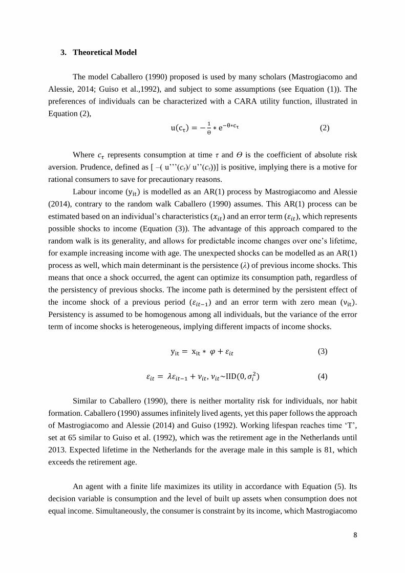
Alessie, 2014; Guiso et al.,1992), and subject to some assumptions (see Equation (1)). The

preferences of individuals can be characterized with a CARA utility function, illustrated in

Equation (2),

u(cτ) = −1

ϴ∗ e−θ∗cτ (2)

Where 𝑐𝜏 represents consumption at time τ and ϴ is the coefficient of absolute risk

aversion. Prudence, defined as [ –( u’’’(cτ)/ u’’(cτ))] is positive, implying there is a motive for

rational consumers to save for precautionary reasons.

Labour income (yit) is modelled as an AR(1) process by Mastrogiacomo and Alessie

(2014), contrary to the random walk Caballero (1990) assumes. This AR(1) process can be

estimated based on an individual’s characteristics (𝑥𝑖𝑡) and an error term (𝜀𝑖𝑡), which represents

possible shocks to income (Equation (3)). The advantage of this approach compared to the

random walk is its generality, and allows for predictable income changes over one’s lifetime,

for example increasing income with age. The unexpected shocks can be modelled as an AR(1)

process as well, which main determinant is the persistence (λ) of previous income shocks. This

means that once a shock occurred, the agent can optimize its consumption path, regardless of

the persistency of previous shocks. The income path is determined by the persistent effect of

the income shock of a previous period (𝜀𝑖𝑡−1) and an error term with zero mean (νit).

Persistency is assumed to be homogenous among all individuals, but the variance of the error

term of income shocks is heterogeneous, implying different impacts of income shocks.

yit = xit ∗ 𝜑 + 𝜀𝑖𝑡 (3)

𝜀𝑖𝑡 = 𝜆𝜀𝑖𝑡−1 + 𝜈𝑖𝑡, 𝜈𝑖𝑡~IID(0, 𝜎𝑖2) (4)

Similar to Caballero (1990), there is neither mortality risk for individuals, nor habit

formation. Caballero (1990) assumes infinitely lived agents, yet this paper follows the approach

of Mastrogiacomo and Alessie (2014) and Guiso (1992). Working lifespan reaches time ‘T’,

set at 65 similar to Guiso et al. (1992), which was the retirement age in the Netherlands until

2013. Expected lifetime in the Netherlands for the average male in this sample is 81, which

exceeds the retirement age.

An agent with a finite life maximizes its utility in accordance with Equation (5). Its

decision variable is consumption and the level of built up assets when consumption does not

equal income. Simultaneously, the consumer is constraint by its income, which Mastrogiacomo

9

and Alessie (2014) formulate according to Equation (6). 𝐴𝑡−1 is last year’s level of assets and

r is the discount rate. The left-hand side illustrates total lifetime consumption, and the righthand

side total assets over a lifetime.

max Et [∑u(cτ)

(1+ρ)τ−tTτ=t ] (5)

∑cτ

(1+r)τ−tTτ=t = (1 + r)At−1 + ∑

yτ

(1+r)τ−tTτ=t (6)

At time τ=0, one starts with zero assets, as any assets accumulated before would be

bequests from parents, which do not origin from own labour income. Due to both not allowing

for negative assets at time T and no bequest motive, assets equal zero at time T.

Due to mental accounting, housing wealth is often regarded as retirement savings, and

individuals do not consume out of this wealth (Mastrogiacomo and Alessie, 2011). By

excluding housing wealth from the restriction of zero assets at time T, agents do not take zero

assets into retirement. Additionally, Paiella (2007) found that propensity to consume out of

wealth gains was minimal for housing wealth. Heaton and Lucas (1997) argue that people invest

in financial assets to protect themselves against income shocks and Hockguertel (2003) finds

that people invest more in safe liquid assets if exposed to more uncertainty. Therefore, the main

regression will focus on financial wealth, which is more likely to be used for precautionary

reasons, whereas the illiquid assets are more likely to be used for retirement purposes.

A closed form solution to the maximization problem in Equation (6) is found by solving

the Euler Equation, when time preference equals the discount rate and time separability of

utility holds.

∂u(ct)

∂ct= Et [

∂u(ct+1)

∂ct+1] (7)

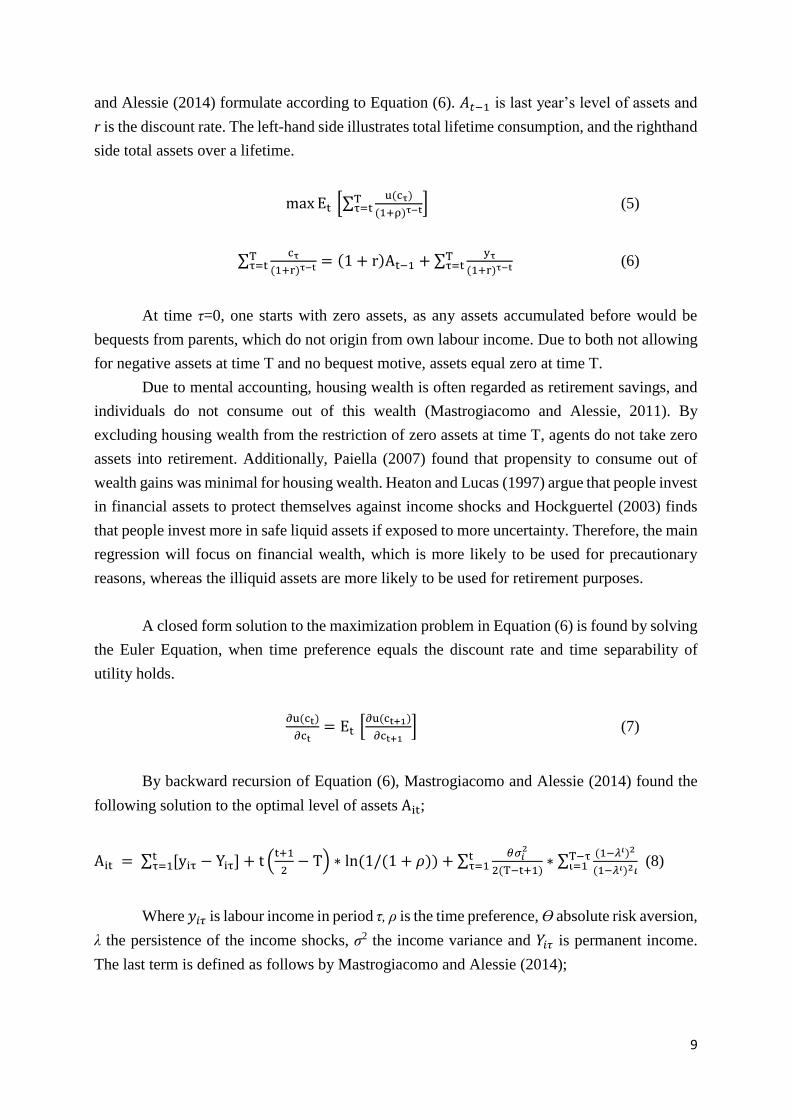
By backward recursion of Equation (6), Mastrogiacomo and Alessie (2014) found the

following solution to the optimal level of assets Ait;

Ait = ∑ [yiτ − Yiτtτ=1 ] + t (

t+1

2− T) ∗ ln(1/(1 + 𝜌)) + ∑

𝜃𝜎𝑖2

2(T−t+1)

tτ=1 ∗ ∑

(1−𝜆𝜄)2

(1−𝜆𝜄)2𝜄

T−τι=1 (8)

Where 𝑦𝑖𝜏 is labour income in period τ, ρ is the time preference, ϴ absolute risk aversion,

λ the persistence of the income shocks, σ2 the income variance and 𝑌𝑖𝜏 is permanent income.

The last term is defined as follows by Mastrogiacomo and Alessie (2014);

10

Yit = (T − t + 1)−1 ∗ (Ait−1 + ∑ EityiτTτ=1 ) (9)

𝑤𝑖𝑡ℎ 𝐴𝑖𝑡−1 representing the assets of the previous year and 𝐸𝑖𝑡𝑦𝑖𝜏 are the expectations

at time t of all future income. It is assumed that at time t the expectations for all future income

streams are equivalent to the expected income of the next year. These expectations can be

altered each period.

In this paper, the definition of permanent income is modified, since Equation (9) yields

multiple negative or economically infeasibly low values of permanent income. Similar to Guiso

et al. (1992), the term ‘permanent earnings’ is used to emphasizing the focus on the earnings

uncertainty of the labour force, regardless of their working status. Guiso et al. (1992) assumed

dynamic income levels, which depend on an individual’s characteristics, such as age and

education. This paper simplifies the model of Guiso et al. (1992), constructing permanent

earnings (𝑌𝑖𝑡) as a function of recent net income and the number of future labour earnings that

left, which depends on age;

𝑌𝑖𝑡 = (𝑦𝑖𝑡 + (65 − 𝐴𝑔𝑒𝑖𝑡) ∗ (𝐸𝑖𝑡[𝑦𝑖𝑡+1]))/(66 − 𝐴𝑔𝑒𝑖𝑡) (10)

With yit being household net income, and 𝐸𝑖𝑡[𝑦𝑖𝑡+1] representing next year’s expected

household net income, which is assumed to be the expected income level for all future periods.

Without uncertainty or prudence, one consumes permanent income every year, and the

difference between current income and permanent income determines the level of assets/

liabilities. This is portrayed by the first term in Equation (8) and together with the second term,

which represents impatience, the optimal solution without prudence and uncertainty would be

obtained. The third term depicts the precautionary motive, which increases assets. When

uncertainty, risk aversion or persistence of the shocks increases, precautionary savings increase.

An effect that is solely found in a model with finite time is the dependency on age. For

those who have already built up many assets and only have a small period of exposure to income

risk remaining, exhibition of precautionary behavior is less likely. A younger individual, who

still has an extended period of income risk exposure and has not accumulated many assets yet,

is more likely to exhibit precautionary behavior. In infinite time models one faces uncertainty

for an infinite period of time, diminishing the influence of age.

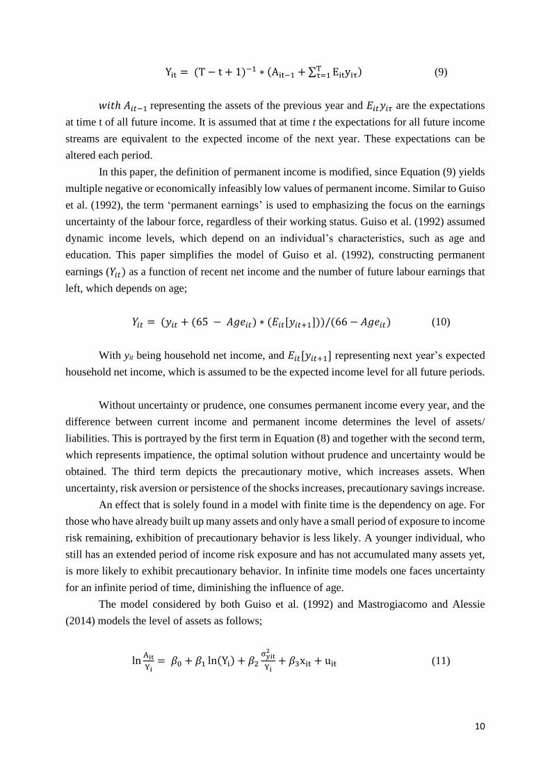
The model considered by both Guiso et al. (1992) and Mastrogiacomo and Alessie

(2014) models the level of assets as follows;

lnAit

Yi= 𝛽0 + 𝛽1 ln(Yi) + 𝛽2

σyit2

Yi+ 𝛽3xit + uit (11)

11

The dependent variable is the log of assets divided by permanent earnings. The right-

hand side contains the log of permanent earnings ln(Yi), the conditional variance of income

variance divided by permanent earnings (σit2 /Yi), a vector of controls 𝑥𝑖𝑡 and the error term uit.

The model in this paper is based on Equation (11), yet with the extension that the income

variance is dependent on the time-period. D denotes the dummy for either pre-crisis period or

post-crisis period and ϴ is the dummy for being risk averse.

lnAit

Yi= 𝛽0 + 𝛽1 ln(Yi) + 𝛽2Dcrisis

σit2

Yi+ 𝛽3𝐷𝑐𝑟𝑖𝑠𝑖𝑠 + 𝛽4𝜃it + 𝛽5xit + uit (12)

4. Data

In this paper use is made of data of the DNB Household Survey administered by

CentERdata (Tilburg University, The Netherlands). The survey is annually distributed amongst

a representative sample of the Dutch population since 1993. For this study, the waves of the

year 20042 till 2017 are used, in which information on the previous and current year is asked.

The Great Recession started at the end of 2007 and ended in 2008. For Europe, this was

followed by the Solvency Crisis until 2010 and followed up by the European Debt Crisis until

and including 2013. During the third quarter of 2015, the CBS3 concluded that the Netherlands

had overcome the crisis with growth in many domestic sectors compared to the previous year.

Therefore, 2015 has been assumed to be the first year of post-crisis. This results in four years

of pre-crisis, seven years of economic downturn, and two years of post-crisis. The 7-year period

will be referred to as the ‘crisis period’.

During this period, information on 60,855 individuals was gathered, of which 25,379

were the heads of the household. Annually, between 1,600 and 2,300 households responded to

the survey. Unfortunately, not all respondents have filled out the annual survey satisfactory,

hence a large amount of observations had to be dropped for which relevant information is

unknown. One cause of missing information is the distribution of the sub-questionnaire during

different periods of the year. Missing data on gender and birthyear could be reconstructed when

this information was provided consistently in another year. For education, missing values could

be filled up when the highest obtained education of the year before and after is known, and

those levels were identical.

Due to non-response, addition of new households and inconsistency of relevant

questions, the unbalanced panel data set is reduced to 3,097.4 Annually, between 200 and 300

households can be used for the analysis. This sample includes 1,034 unique households which

remain 4.6 years in the sample on average, with a maximum of 14 appearances. The paper uses

four sample sizes; the main sample, a second sample with alternative measure of income risk;

2 Data of 2003 used to calculate lags for 2004. 3 https://www.rtlz.nl/algemeen/economie/cbs-crisis-lijkt-achter-ons 4 Deviating values regarding; expected income changes, net income, net worth, financial wealth or the ranges for

next year’s income and resulted in 26 exclusions.

12

one with the additional controls; and the fourth with both additional controls and the alternative

uncertainty measure.5 The three other samples are smaller in size; respectively containing

3,014, 1,794, and 1,717 observations.

4.1 Variable construction

Assets

Like Mastrogiacomo and Alessie (2014), who make use of different waves of the DHS

data set, net worth is calculated as the addition of all assets and subtraction of liabilities. For

financial worth, mortgages, real-estate, and other illiquid assets such as boats were not included.

Unfortunately, the survey does not ask for each item which member(s) of the household is/are

the owner(s), only for deposits, checking-accounts, and savings the survey provides this

information. Arrears, mortgages, and real estate are assumed to be owned by all members of

the household, who are assumed to be equally responsible for housing assets. For other items,

it was assumed that they were individually owned, unless the household members provided the

same value. Furthermore, if the exact level of assets or liabilities is not known by the

respondents, they are offered value ranges in which they can scale their assets/ liability. The

midpoint of this range is used in that case. Some questions on assets have been adjusted, added

or deleted. An overview of the construction and adjustments can be found in Appendix A.

Permanent Earnings & head of household

Equation (10) defines the value of permanent earnings, which is defined as an average

of current household net income and the expectations of the head of the household of next year’s

net income. Section 4.2 elaborates on the expected future income level. The head of household

has been determined based upon a question regarding financial decision making within the

household. If this question yielded no dominant decider, the person who was registered as head

of household was considered as the head of household.

Risk aversion & Crisis Dummies

A respondent is asked to provide a number within a scale of 1-7 to rate how much they

agree with the statement, with ‘1’ representing totally disagree and ‘7’ totally agree with a

question regarding risk averseness. As the crisis might affect risk, risk aversion is not assumed

to be time-invariant, and changes are thus allowed. Most respondents only change their answers

remotely, yet each year a small group changes drastically. Table 1 shows that the average

change per head did not differ more around the crisis years. When a respondent altered their

answer to the risk aversion question with one-point difference compared to the previous year,

it does not necessarily mean that risk aversion changes. Out of the 2,502 people of whom a

5 Reduced size due to missing information or questions not annually occurring

13

previous risk aversion score is known, 2.005 have changed their score.6 When a respondent

answered with a 5 or higher, they are considered to be risk averse.7 About one third of the

observations changed more than twice from being risk averse to not risk averse or vice versa

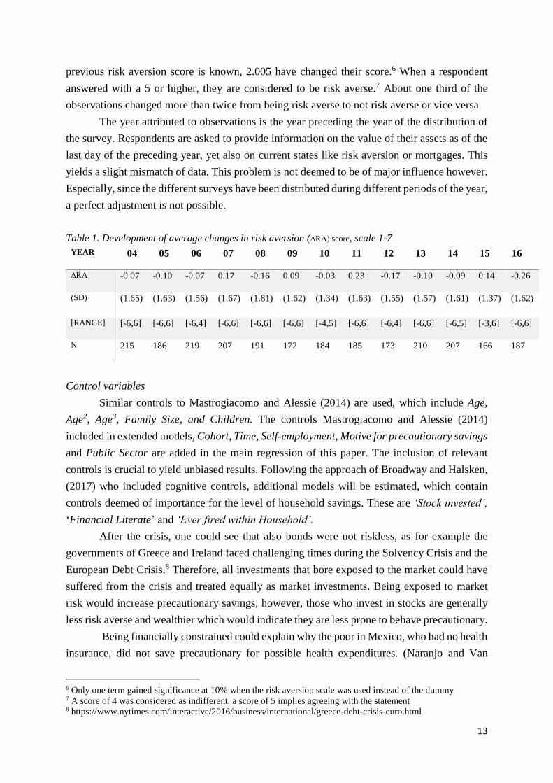
The year attributed to observations is the year preceding the year of the distribution of

the survey. Respondents are asked to provide information on the value of their assets as of the

last day of the preceding year, yet also on current states like risk aversion or mortgages. This

yields a slight mismatch of data. This problem is not deemed to be of major influence however.

Especially, since the different surveys have been distributed during different periods of the year,

a perfect adjustment is not possible.

Table 1. Development of average changes in risk aversion (∆RA) score, scale 1-7

YEAR 04 05 06 07 08 09 10 11 12 13 14 15 16

∆RA -0.07 -0.10 -0.07 0.17 -0.16 0.09 -0.03 0.23 -0.17 -0.10 -0.09 0.14 -0.26

(SD)

(1.65) (1.63) (1.56) (1.67) (1.81) (1.62) (1.34) (1.63) (1.55) (1.57) (1.61) (1.37) (1.62)

[RANGE] [-6,6] [-6,6] [-6,4] [-6,6] [-6,6] [-6,6] [-4,5] [-6,6] [-6,4] [-6,6] [-6,5] [-3,6] [-6,6]

N 215 186 219 207 191 172 184 185 173 210 207 166 187

Control variables

Similar controls to Mastrogiacomo and Alessie (2014) are used, which include Age,

Age2, Age3, Family Size, and Children. The controls Mastrogiacomo and Alessie (2014)

included in extended models, Cohort, Time, Self-employment, Motive for precautionary savings

and Public Sector are added in the main regression of this paper. The inclusion of relevant

controls is crucial to yield unbiased results. Following the approach of Broadway and Halsken,

(2017) who included cognitive controls, additional models will be estimated, which contain

controls deemed of importance for the level of household savings. These are ‘Stock invested’,

‘Financial Literate’ and ‘Ever fired within Household’.

After the crisis, one could see that also bonds were not riskless, as for example the

governments of Greece and Ireland faced challenging times during the Solvency Crisis and the

European Debt Crisis.8 Therefore, all investments that bore exposed to the market could have

suffered from the crisis and treated equally as market investments. Being exposed to market

risk would increase precautionary savings, however, those who invest in stocks are generally

less risk averse and wealthier which would indicate they are less prone to behave precautionary.

Being financially constrained could explain why the poor in Mexico, who had no health

insurance, did not save precautionary for possible health expenditures. (Naranjo and Van

6 Only one term gained significance at 10% when the risk aversion scale was used instead of the dummy 7 A score of 4 was considered as indifferent, a score of 5 implies agreeing with the statement 8 https://www.nytimes.com/interactive/2016/business/international/greece-debt-crisis-euro.html

14

Gameren, 2016). Following Collins (2012), financial advice cannot substitute financial literacy,

it can only complement financial literacy. If one is less financially educated, one is less able to

make optimal financial decisions, resulting in insufficient self-insurance.

An effect of the crisis was the increase in unemployment.9 Therefore, a variable is

constructed to see whether one of the two spouses has been fired until that point in time, based

on working status. When one faced an income shock, resources had to be depleted and might

be more prone to future precautionary savings (Broadway and Halsken, 2017).

Cohorts are constructed per decade, starting with cohort1, which includes those born

between 1985 - 1994. Someone born in 1994 would be legally responsible for their own

finances in the Netherlands in 2017, which is the year of the last collection of data. Six cohorts

are constructed in total. The oldest cohort drops out of the sample when the crisis starts. Older

cohorts are assumed to have retired in this model, thus cannot provide any data on their earnings

variance.

Motivation to save for unexpected expenses is used as control variable as the crisis could

affect one’s opinion on precautionary savings. The bequest motive which Mastrogiacomo and

Alessie (2014) included has been deterred from the model. Rossi and Sansone (2017) studied

the effect of uncertainty on the level of bequest levels in Italy in the period of 2004-2012 and

found no effect. See appendix A for further information on the construction of variables.

Ideally, expected real income changes should be considered, as opposed to nominal

changes used in this paper. The survey asks individuals to present their expectations on price

changes, yet the phrasing of the question regarding the inflation has been changed. Up and until

including 2007, one could provide any expected inflation rate, similarly to the question

regarding expectations on income. From 2008 onwards, the survey asks respondents how likely

they think it is that prices change within the range of [0% - 15%]. Answers to the initial question

regarding inflation yielded answers exceeding both limits provided by the latter question, yet

the biggest objection against using both data sets is a bias of getting predetermined inflation

rates or having to determine yourself. This would lead to a bias. Additionally, inflation rates

have been historically low during this period, with an average of 1.65%.10 Similar to

Mastrogiacomo and Alessie (2014), the inflation rate has not been accounted for.

4.2 Earnings Variance

Subjective earnings variance is based upon the survey question asking respondents to

provide the highest and lowest expected income level on the household level for upcoming year.

The variable of earnings variance was based upon the following question until 2008:

9 https://www.volkskrant.nl/economie/werkloosheid-daalt-maar-is-nog-altijd-hoger-dan-voor-crisis-vooral-

mannen-vinden-moeilijk-baan~b592378e/ 10 http://nl.inflation.eu/inflatiecijfers/nederland/historische-inflatie/cpi-inflatie-nederland.aspx

15

“We would like to know a little bit more about what you expect will happen to the net income

of your household in the next 12 months. What do you expect to be the LOWEST total net

monthly income your household may realize in the next 12 months? (=LAAG)… What do you

expect to be the HIGHEST total net income your household may realize in the next 12

months?(=HOOG)”

“Below, we will show you a number of amount that could theoretically be the total net income

of your household. Please indicate with each amount what you think is the probability [..] that

the total net income of your household will be LESS than this amount in the next 12 months.”

“What do you think is the probability that the total net income of your household will be less

than €[LAAG+((HOOG-LAAG)*({2,4,6,8}))/10] in the next 12 months?”

The above stated question is not clear, the first sub-question asks for monthly income

and the second sub-question for annual income. After 2008, the question was rephrased as

follows:

‘What do you expect to be the LOWEST total net yearly income your household may realize in

the next 12 months?’

The average expected income, assuming annual incomes were provided, was €18,976

before 2008 and €35,284 after. Equation (16) elaborates on the construction of expected

income. Based upon visual judgement (Appendix C) the difference between before and after the

rephrasing of the question is also clear.11 There is a range in which hardly any values are situated

around €5,000.-. Expected incomes below €5,000.- before 2008 were assumed to be monthly

income estimations and these incomes have been multiplied by 12. An annual income of

€5,000.- is very low, especially considering that the gross minimum wage is around €1,500.-

per month12. One cannot presume all respondents filled out monthly data in preceding years,

due to part-time work for example. Yet, for those who have been assumed to have provided

monthly data before 2008 and still provide income levels below €5,000.-, the assumption is

made these respondents repeatedly filled out the questionnaire wrong.13 Those who had an

expected income lower than €100, which was simultaneously lower than last year’s income

divided by 12 were dropped.

If a respondent thinks it will earn at least €100 (LAAG/income00) and a maximum of

€200 (HOOG/income100), they are asked to provide the probability of earning at least €120

(income20), €140 (income40), €160 (income60) and €180 (income80). The probabilities of

earning these incomes are denoted as pro1, pro2, pro3, and pro4 respectively. The probability

11 Of all observations with expected lower income than €10,000.-, 80% was in the period of 2004-2007. 12 Gross minimum in 2010; https://www.plusonline.nl/werken/uitkeringen-per-1-januari-2010 13 These changes have been made for 808 individuals before 2008 and 66 from 2008 onwards (Main sample)

16

of earning at least income00, is equal to zero. The chance on one specific value on a continuous

scale is zero. The probability of earning at least income100 is equal to 100%.

To be consistent, the probabilities should satisfy the following conditions; The

probabilities cannot descent to sustain increasing monotonicity; pro1 has to exceed 0, otherwise

income00 is not the lowest expected income; pro1-pro4 cannot be 100%, otherwise income100

cannot be obtained. Two alternate answer strategies were found under the respondents for which

the answers are still valid.

• When the increasing monotonicity assumption was violated, one could have also

answered the question by focusing on the smaller income ranges separately instead of

the whole area on the left of the suggested income level. They focus on the 20% income

ranges instead of adding the probabilities e.g. provide the probability of earning between

€100-€120 and €120-€140 instead of between €100-€120 and €100-€140.

If the total sum of separate probabilities attained a maximum of 99%, this alternative

approach is used.

• When strictly descending probabilities were provided, which also exceeded 99% if

added, they were assumed to have switched the distribution around. If the first

probability is 90% and the second 80%, it is assumed that the respondent believes that

there is a 90% probability that he or she will earn at least €120 and a probability of 80%

of earning at least €140. These answers have been altered by proposing that being 90%

sure of earning at least this amount is equal to being 10% sure that €120 is the maximum

and thus earning at least €120.14

Due to inconsistency under all three methods, 719 observations had to be dropped. Dominitz

and Manski (1997) studied the strength of this measure with “LAAG”, “HOOG” questions for

income uncertainty and found that it was a feasible and useful measure of income expectations,

yet to be used with caution of incoherent answers.

Earnings variance has been calculated by following the approach of Mastrogiacomo and

Alessie (2014). The respondents in their dataset were asked to rate how likely they deem relative

income changes within a range of [-15%,+15%]. To calculate these relative income changes

(∆𝜍 )for the sample in this paper, this year’s net income (yit) is subtracted from the five possible

income levels based upon the question stated above. These expected income

values (𝑖𝑛𝑐𝑜𝑚𝑒𝜍0) are set at the midpoint of the lower bound and the upper bound of each 20%

range. The difference of the net income and expected income value is divided by net income

(yit), see Equation (14). Calculating the total expected income change is done by multiplying

the expected percentage change by the probabilities of obtaining these expected income values.

To obtain these percentages, the probabilities were cut into smaller pieces, similar to the first

alternative answer strategy. By subtracting the probability of earning 20% more from the initial

14 The probability of earning a precise amount on a continues scale is zero.

17

value, the probability of earning the expected income value is calculated (𝑝𝑟𝑜20/40/60/80/

100). Equation (13) illustrates the construction of the expected total income change. The

variance of the income change, 𝜎2, is computed with the help of the standard formula of

variance in Equation (15).

E[%∆yit] = ∑ 𝑝𝑟𝑜𝜄 ∗ 𝐸[∆𝜍] for ι = 20,40,60,80,100 & ς=1,2,3,4,5 (13)

E[∆𝜍] = (𝑖𝑛𝑐𝑜𝑚𝑒𝜍0 − 𝑦𝑖𝑡)/𝑦𝑖𝑡 ,where ς=1,2,3,4 or 5 (14)

σ2 = ∑ proι0 ∗ (𝐸[∆𝜍] − E[%∆yit])2

for ι = 2,4,6,8,10 & ς = 0,2,4,6,8 (15)

To find the conditional variance (𝜎𝑦2), one needs to multiply the variance with the square

of current income, σ2 ∗ yit2 . The measure of conditional variance divided by permanent earnings

(σ2yit /Yit) is the initial estimate of earnings variance within this paper.

Expected income for the next period is calculate by multiplying the expected income

values (𝑖𝑛𝑐𝑜𝑚𝑒𝜍0) with the probability of net income being situated within that income

range(proι0);

E[𝑦𝑡+1] = ∑ proι0 ∗ 𝑖𝑛𝑐𝑜𝑚𝑒𝜍0 for ι = 20,40,60,80,100 & ς=1,2,3,4,5 (16)

Whereas to Mastrogiacomo and Alessie (2014) found a mean ratio of the standard

deviation of future income to current income (σyit/yit) of 3%, this paper finds 9.43%. The

individuals in this sample have slight pessimistic expectations for their future income. The

average increase in earnings is 36.86%, with an expected earnings variance of 4.46%. When

the 118 individuals who believe their income exceeds this year’s at least with 100% are ignored,

the average income change is -2.5%. The value of (σy/yit) drops to 7.04%, which is still quite

high compared to Mastrogiacomo and Alessie (2014). When the observations of which the

minimum or maximum expected change in income exceeded [-15%-15%], which are the ranges

the respondents faced in the data of Mastrogiacomo and Alessie (2014), 1,887 observations are

left, who have an expected income change of 0.06% with (σyit/yit) dropping to 5.55%. The

average expected income for next year is €33,886 compared to the average income of €36,335

of the previous year. The questions regarding income expectations follow shortly after the

questions regarding current net income, which increases the likelihood of proper expectations.

18

4.2.1 Variance unemployment risk

As Kennickell and Lusardi (2004) argued, the shortcoming of the approach above is the

inability of one year ahead income variance to capture lifetime income risks. Mastrogiacomo

and Alessie (2014) use length of entitlement to unemployment benefits as instrument for

income risk. Since Dutch employment contracts specify predetermined wages, the main

uncertainty for workers is being fired. This paper uses the subjective probability of being

without a job next year as alternative measurement of earnings variance. Those who were

employed had to answer the first question, those who are unemployed but looking the second;

“What do you think is the probability that you lose your job in the next 12 months?”

“What do you think is the probability that you find a job in the next 12 months?”

For those who were not currently employed but were searching for a job, the probability

of being without a job (pJL) in the next period is determined by subtracting the chance of getting

a job from 100%.

Respondents who are certain they will lose their job next year face lower expected

income, however face no uncertainty. Therefore, the variance of the chance of being

unemployed next year must be estimated. For binomial distributions, this is done by using

Equation (17);

var(𝑝𝐽𝐿) = 1 ∗ (1 − 𝑝𝐽𝐿) (17)

Mastrogiacomo and Alessie (2014) have shown that the uncertainty of the spouse is of

importance as well. The relevant question only had to be answered by those working or looking

for a job, e.g. the working population. Most spouses were voluntary not working, thus the

chance of an income shock through them is zero. The alternative measure of earnings risk is

estimated as the variance of the chance of at least one of both spouses having zero income out

of labour next year. The chance of at least one household member being jobless (pJLHH) is

estimated by Equation (18), in which pJLH is the head’s subjective probability of being without

a job next year and pJHS is the equivalent for the spouse.15 The corresponding variance,

var(pJLHH), is calculated similar to Equation (17).

𝑝𝐽𝐿𝐻𝐻 = [1 − (1 − 𝑝𝐽𝐿𝐻) ∗ (1 − 𝑝𝐽𝐿𝑆)] (18)

15 Assuming zero correlation between both events.

19

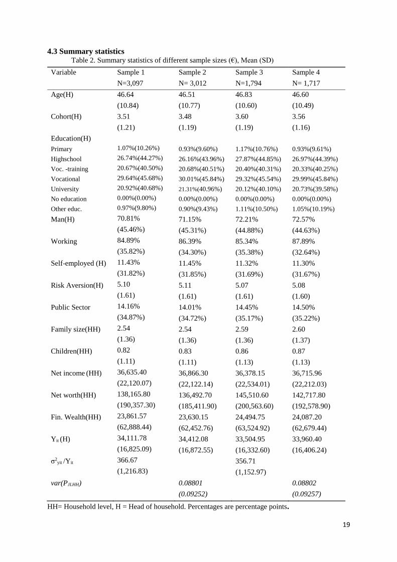
4.3 Summary statistics Table 2. Summary statistics of different sample sizes (€), Mean (SD)

Variable Sample 1

N=3,097

Sample 2

N= 3,012

Sample 3

N=1,794

Sample 4

N= 1,717

Age(H)

Cohort(H)

Education(H)

Primary

Highschool

Voc. -training

Vocational

University

No education

Other educ.

Man(H)

Working

Self-employed (H)

Risk Aversion(H)

Public Sector

Family size(HH)

Children(HH)

Net income (HH)

Net worth(HH)

Fin. Wealth(HH)

Yit (H)

σ2yit /Yit

var(PJLHH)

46.64

(10.84)

3.51

(1.21)

1.07%(10.26%)

26.74%(44.27%)

20.67%(40.50%)

29.64%(45.68%)

20.92%(40.68%)

0.00%(0.00%)

0.97%(9.80%)

70.81%

(45.46%)

84.89%

(35.82%)

11.43%

(31.82%)

5.10

(1.61)

14.16%

(34.87%)

2.54

(1.36)

0.82

(1.11)

36,635.40

(22,120.07)

138,165.80

(190,357.30)

23,861.57

(62,888.44)

34,111.78

(16,825.09)

366.67

(1,216.83)

46.51

(10.77)

3.48

(1.19)

0.93%(9.60%)

26.16%(43.96%)

20.68%(40.51%)

30.01%(45.84%)

21.31%(40.96%)

0.00%(0.00%)

0.90%(9.43%)

71.15%

(45.31%)

86.39%

(34.30%)

11.45%

(31.85%)

5.11

(1.61)

14.01%

(34.72%)

2.54

(1.36)

0.83

(1.11)

36,866.30

(22,122.14)

136,492.70

(185,411.90)

23,630.15

(62,452.76)

34,412.08

(16,872.55)

0.08801

(0.09252)

46.83

(10.60)

3.60

(1.19)

1.17%(10.76%)

27.87%(44.85%)

20.40%(40.31%)

29.32%(45.54%)

20.12%(40.10%)

0.00%(0.00%)

1.11%(10.50%)

72.21%

(44.88%)

85.34%

(35.38%)

11.32%

(31.69%)

5.07

(1.61)

14.45%

(35.17%)

2.59

(1.36)

0.86

(1.13)

36,378.15

(22,534.01)

145,510.60

(200,563.60)

24,494.75

(63,524.92)

33,504.95

(16,332.60)

356.71

(1,152.97)

46.60

(10.49)

3.56

(1.16)

0.93%(9.61%)

26.97%(44.39%)

20.33%(40.25%)

29.99%(45.84%)

20.73%(39.58%)

0.00%(0.00%)

1.05%(10.19%)

72.57%

(44.63%)

87.89%

(32.64%)

11.30%

(31.67%)

5.08

(1.60)

14.50%

(35.22%)

2.60

(1.37)

0.87

(1.13)

36,715.96

(22,212.03)

142,717.80

(192,578.90)

24,087.20

(62,679.44)

33,960.40

(16,406.24)

0.08802

(0.09257)

HH= Household level, H = Head of household. Percentages are percentage points.

20

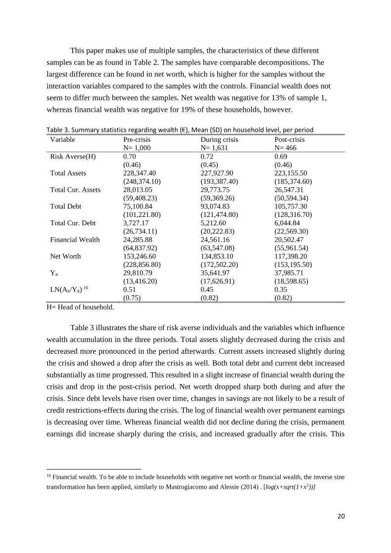
This paper makes use of multiple samples, the characteristics of these different

samples can be as found in Table 2. The samples have comparable decompositions. The

largest difference can be found in net worth, which is higher for the samples without the

interaction variables compared to the samples with the controls. Financial wealth does not

seem to differ much between the samples. Net wealth was negative for 13% of sample 1,

whereas financial wealth was negative for 19% of these households, however.

Table 3. Summary statistics regarding wealth (€), Mean (SD) on household level, per period

Variable Pre-crisis

N= 1,000

During crisis

N= 1,631

Post-crisis

N= 466

Risk Averse(H)

0.70

(0.46)

0.72

(0.45)

0.69

(0.46)

Total Assets

Total Cur. Assets

228,347.40

(248,374.10)

28,013.05

(59,408.23)

227,927.90

(193,387.40)

29,773.75

(59,369.26)

223,155.50

(185,374.60)

26,547.31

(50,594.34)

Total Debt

Total Cur. Debt

75,100.84

(101,221.80)

3,727.17

(26,734.11)

93,074.83

(121,474.80)

5,212.60

(20,222.83)

105,757.30

(128,316.70)

6,044.84

(22,569.30)

Financial Wealth 24,285.88

(64,837.92)

24,561.16

(63,547.08)

20,502.47

(55,961.54)

Net Worth

Yit

153,246.60

(228,856.80)

29,810.79

(13,416.20)

134,853.10

(172,502.20)

35,641.97

(17,626.91)

117,398.20

(153,195.50)

37,985.71

(18,598.65)

LN(Ait/Yit) 16

0.51

(0.75)

0.45

(0.82)

0.35

(0.82)

H= Head of household.

Table 3 illustrates the share of risk averse individuals and the variables which influence

wealth accumulation in the three periods. Total assets slightly decreased during the crisis and

decreased more pronounced in the period afterwards. Current assets increased slightly during

the crisis and showed a drop after the crisis as well. Both total debt and current debt increased

substantially as time progressed. This resulted in a slight increase of financial wealth during the

crisis and drop in the post-crisis period. Net worth dropped sharp both during and after the

crisis. Since debt levels have risen over time, changes in savings are not likely to be a result of

credit restrictions-effects during the crisis. The log of financial wealth over permanent earnings

is decreasing over time. Whereas financial wealth did not decline during the crisis, permanent

earnings did increase sharply during the crisis, and increased gradually after the crisis. This

16 Financial wealth. To be able to include households with negative net worth or financial wealth, the inverse sine

transformation has been applied, similarly to Mastrogiacomo and Alessie (2014) . [log(x+sqrt(1+x2))]

21

rapid increase could be the result of the vague question regarding monthly/ annual income

expectations.

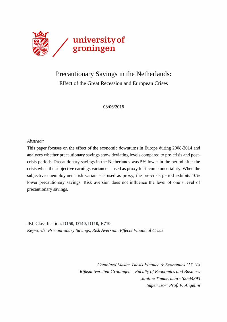
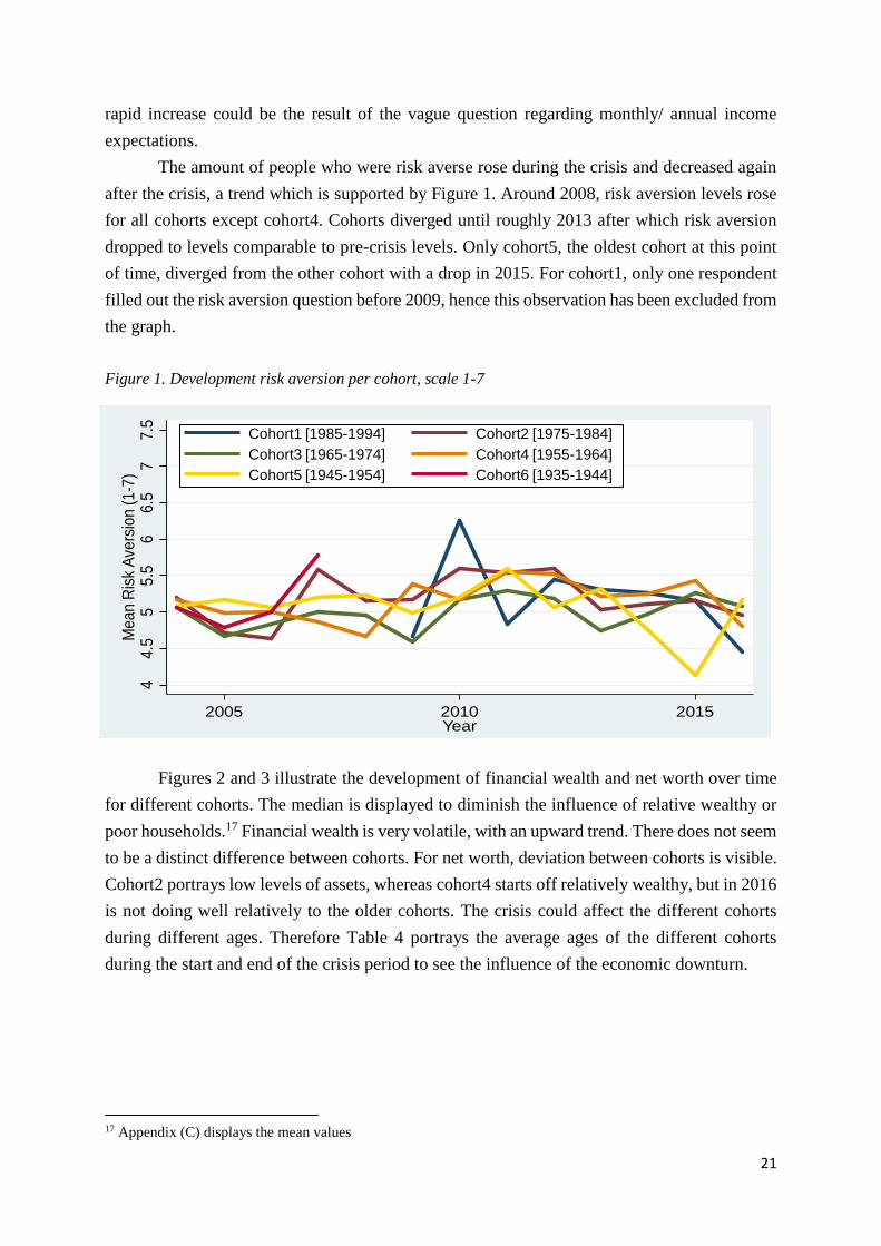
The amount of people who were risk averse rose during the crisis and decreased again

after the crisis, a trend which is supported by Figure 1. Around 2008, risk aversion levels rose

for all cohorts except cohort4. Cohorts diverged until roughly 2013 after which risk aversion

dropped to levels comparable to pre-crisis levels. Only cohort5, the oldest cohort at this point

of time, diverged from the other cohort with a drop in 2015. For cohort1, only one respondent

filled out the risk aversion question before 2009, hence this observation has been excluded from

the graph.

Figure 1. Development risk aversion per cohort, scale 1-7

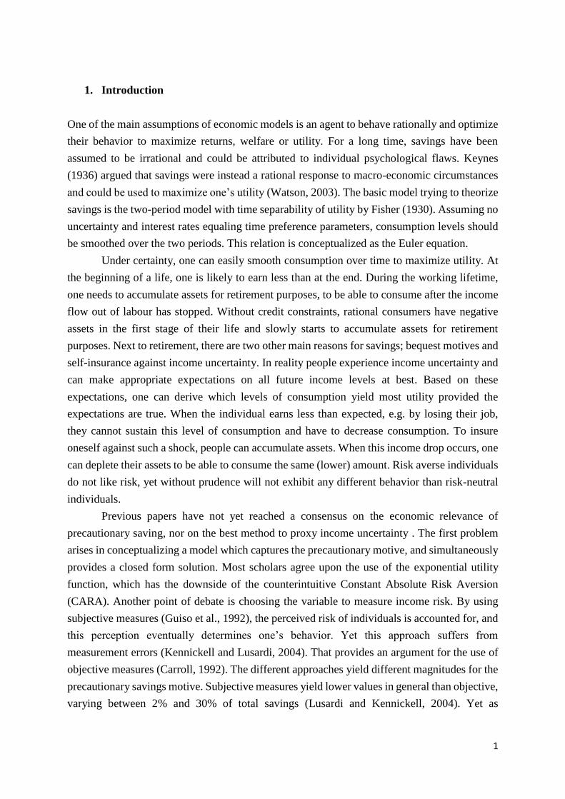
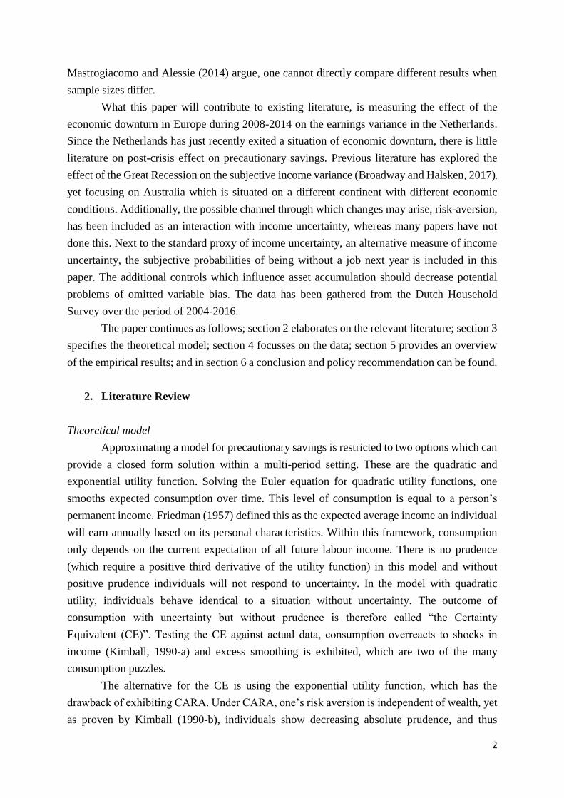
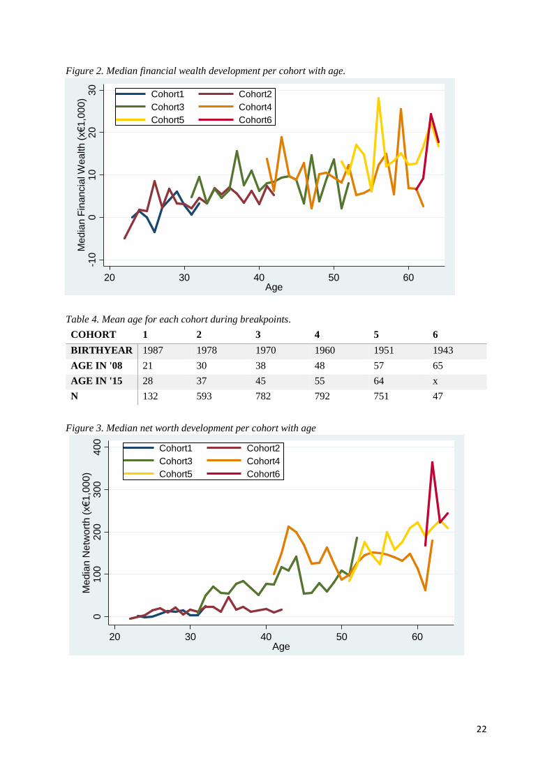
Figures 2 and 3 illustrate the development of financial wealth and net worth over time

for different cohorts. The median is displayed to diminish the influence of relative wealthy or

poor households.17 Financial wealth is very volatile, with an upward trend. There does not seem

to be a distinct difference between cohorts. For net worth, deviation between cohorts is visible.

Cohort2 portrays low levels of assets, whereas cohort4 starts off relatively wealthy, but in 2016

is not doing well relatively to the older cohorts. The crisis could affect the different cohorts

during different ages. Therefore Table 4 portrays the average ages of the different cohorts

during the start and end of the crisis period to see the influence of the economic downturn.

17 Appendix (C) displays the mean values

44.

55

5.5

66.

57

7.5

Mea

n R

isk

Ave

rsio

n (1

-7)

2005 2010 2015Year

Cohort1 [1985-1994] Cohort2 [1975-1984]Cohort3 [1965-1974] Cohort4 [1955-1964]Cohort5 [1945-1954] Cohort6 [1935-1944]

44.

55

5.5

66.

57

7.5

Mea

n R

isk

Ave

rsio

n (1

-7)

2005 2010 2015Year

Cohort1 [1985-1994] Cohort2 [1975-1984]Cohort3 [1965-1974] Cohort4 [1955-1964]Cohort5 [1945-1954] Cohort6 [1935-1944]

22

Figure 2. Median financial wealth development per cohort with age.

Table 4. Mean age for each cohort during breakpoints.

COHORT 1 2 3 4 5 6

BIRTHYEAR 1987 1978 1970 1960 1951 1943

AGE IN '08 21 30 38 48 57 65

AGE IN '15 28 37 45 55 64 x

N 132 593 782 792 751 47

Figure 3. Median net worth development per cohort with age

-10

010

2030

Med

ian

Fin

anci

al W

ealth

(x€

1,00

0)

20 30 40 50 60Age

Cohort1 Cohort2Cohort3 Cohort4Cohort5 Cohort6

010

020

030

040

0M

edia

n N

etw

orth

(x€

1,00

0)

20 30 40 50 60Age

Cohort1 Cohort2Cohort3 Cohort4Cohort5 Cohort6

-10

010

2030

Med

ian

Fin

anci

al W

ealth

(x€

1,00

0)

20 30 40 50 60Age

Cohort1 Cohort2Cohort3 Cohort4Cohort5 Cohort6

-10

010

2030

Med

ian

Fin

anci

al W

ealth

(x€

1,00

0)

20 30 40 50 60Age

Cohort1 Cohort2Cohort3 Cohort4Cohort5 Cohort6

23

Figure 2 illustrates cohort2 obtaining more stability during the crisis. Cohort3 and

cohort4 face a fall in wealth around the start and experience a rather volatile path after the crisis.

Cohort5 and cohort6 face a fall in wealth around the start of the crisis as well.

Cohort1, cohort2, and cohort5 show no outspoken response to the crisis in Figure 3.

Cohort3’s worth increases around the start of the crisis and drops when it ends. Cohort4 and

cohort6 face a drop in net worth around the start, and cohort4 endures another drop in worth

when the crisis ends. The two youngest cohorts illustrate lower levels of net worth. These

cohorts benefited least from the economic boom before the crisis and are thus less equipped

against the economic downturn. The figures show no other pronounced effects of the crisis.

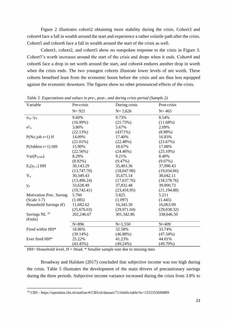
Table 5. Expectations and values in pre-, post-, and during crisis period (Sample 2)

Variable Pre-crisis

N= 921

During crisis

N= 1,626

Post-crisis

N= 465

σyit /yit

σ2it

P(No job t+1) H

P(Jobless t+1) HH

Var(PJLHH)

Eit[yt+1] HH

Yit

yit

Motivation Prec. Saving

(Scale 1-7)

Household Savings (€)

Savings NL 18

(€mln)

9.60%

(16.99%)

3.80%

(22.13%)

14.09%

(21.01%)

15.90%

(22.56%)

8.29%

(8.92%)

30,143.29

(13,747.70)

30,349.43

(13,496.24)

33,628.49

(19,742.41)

5.760

(1.085)

11,682.62

(25,676.03)

202,246.67

9.73%

(21.73%)

5.67%

(4371%)

17.40%

(22.48%)

18.67%

(24.46%)

9.21%

(9.47%)

35,403.36

(18,047.90)

35,675.14

(17,637.76)

37,832.48

(23,416.95)

5.825

(1.097)

16,345.30

(29,971.04)

301,342.86

8.54%

(11.68%)

2.09%

(8.98%)

16.83%

(23.67%)

17.88%

(25.10%)

8.40%

(9.07%)

37,990.43

(19,034.66)

38,042.11

(18,578.76)

39,900.73

(21,194.88)

5.211

(1.445)

16,063.09

(29,038.32)

338,646.50

N=896 N=1,550 N=409

Fired within HH*

18.86%

(39.14%)

32.58%

(46.88%)

33.74%

(47.34%)

Ever fired HH*

25.22%

(43.45%)

41.23%

(49.24%)

44.01%

(49.70%)

HH= Household level, H = Head. * Smaller sample size due to missing data

Broadway and Halsken (2017) concluded that subjective income was too high during

the crisis. Table 5 illustrates the development of the main drivers of precautionary savings

during the three periods. Subjective income variance increased during the crisis from 3.8% to

18 CBS - https://opendata.cbs.nl/statline/#/CBS/nl/dataset/7116shfo/table?ts=1525355690809

24

5.7% and dropped to 2.1% in the post-crisis period. The standard deviation of net income is an

objective measure of income variance, and this increased during the crisis and dropped in the

post-crisis period. The subjective earnings variance moves along with the objective. The head’s

perceived probability of being unemployed next year increases in the crisis period to 17.4% for

the head and drops in the period after the crisis to 16.8%. The probability of either spouse being

unemployed next year corresponds, yet with slightly elevated percentages. The variance of the

probability of being jobless increased during the crisis from 8.3% to 9.2% and decreased to

8.4% in the post-crisis period. Entering the crisis brought along both an increase in the

subjective unemployment variance and an increase of households who had a member lose its

job. After the crisis the subjective risk of unemployment decreased, however the number of

households in which a member lost its job increased slightly. Both proxies of income

uncertainty did rise during the crisis and dropped again afterwards. Expected future income

(Eit[yt+1]) was substantially lower before the crisis and increased with respect to the crisis period

in the post-crisis period. Actual income (yit) rose with time as well, resulting in an increase of

permanent earnings (Yit). The respondent’s motivation for precautionary savings increases a bit

during the crisis, but drops again in the post-crisis period. The level of savings increases during

the crisis, which is found in national data as well. Yet whereas domestic levels increase also

after the crisis, this sample shows a slight decrease. In the three periods, around 52% of the

respondents expected next year’s income to exceed this year’s net income.

5. Empirical Results

The White test and Durbin Watson test find proof for the presence of heteroskedasticity

and autocorrelation in the data. Guiso et al. (1992) acknowledged possible heteroskedasticity

problems and attempted to diminish the problem by dividing the variables by permanent

earnings. This does not solve the problem in this paper and similarly to Guiso et al. (1992)

White standard errors are applied. These error terms adjust for the positive autocorrelation as

well.

Pooled OLS

Similar to Mastrogiacomo and Alessie (2014), Guiso et al. (1992), and Broadway and

Halsken (2017) who use subjective earnings variance, the first regressions are based on pooled

OLS (POLS) models. POLS corrects for within-group different standard errors. The

coefficients are determined similar to cross-sectional data set. For comparability reasons, the

POLS model of Mastrogiacomo and Alessie (2014) is estimated. Their results are quite different

compared to this paper. Their coefficient of subjective earnings variance, b2, is significant at a

1% level, which translates in a precautionary savings rate of 4% of net worth. The identical

regression in this paper yields an insignificant coefficient. The precautionary motive remains

insignificant when financial wealth instead of net wealth is used.

25

Table 6. Regression outputs. Dependent var.: LN(Ait/Yit), POLS, White errors. Proxy: σ2yit

/Yit

VARIABLES (1) ° (2) (3) (4) (5)

LN(Yit) -0.142 0.0385 0.0585 0.0463 -0.0556

(0.0895) (0.0571) (0.0588) (0.0586) (0.0700)

σ2yit

/Yit -3.02e-05 3.17e-06 9.03e-06 6.47e-06 2.26e-05

(2.00e-05) (1.13e-05) (1.74e-05) (1.76e-05) (2.45e-05)

σ2yit

/Yit *Pre -2.40e-05 -2.33e-05 -2.33e-05

(2.10e-05) (2.15e-05) (3.03e-05)

σ2yit

/Yit *Post 8.38e-06 8.14e-06 2.12e-06

(2.89e-05) (2.86e-05) (4.58e-05)

ϴit 0.0961** 0.109**

(0.0409) (0.0452)

Pre-crisis 0.128*** 0.0815 0.0916

(0.0374) (0.0507) (0.0609)

Post-crisis -0.0635 -0.0156 -0.0622

(0.0465) (0.0545) (0.0645)

Age 0.123 0.192* 0.204** 0.178 0.0726

(0.160) (0.101) (0.100) (0.115) (0.132)

Age2 -0.00133 -0.00367 -0.00395* -0.00363 -0.000964

(0.00362) (0.00230) (0.00228) (0.00264) (0.00297)

Age3/102 0.000704 0.00249 0.00270 0.00254 0.000472

(0.00265) (0.00169) (0.00168) (0.00195) (0.00216)

Family Size 0.415*** -0.0392 -0.0455 -0.0403 -0.185**

(0.101) (0.0559) (0.0557) (0.0549) (0.0720)

Children -0.326*** -0.0129 -0.00874 -0.00927 0.101

(0.120) (0.0690) (0.0686) (0.0677) (0.0828)

Self-employed 0.137* 0.0929

(0.0704) (0.0793)

Public-sector 0.157*** 0.147**

(0.0601) (0.0617)

Cohorts Yes Yes

Prec. Motive 0.0133 0.000301

(0.0151) (0.0160)

Stock Invested 0.340***

(0.0576)

Financially

Literate

0.152***

(0.0384)

Fired within HH -0.0466

(0.0500)

Financially

Struggling

-0.210***

(0.0466)

Constant -1.322 -3.296** -3.697** -3.037* -0.924

(2.328) (1.491) (1.491) (1.626) (1.908)

Observations 3,097 3,097 3,097 3,097 1,794

R-squared 0.166 0.069 0.076 0.088 0.145

AIC 10,192 7,204 7,189 7,167 3,993

Joint significance - - -

Significant at ***1%, **5%, *10%. ° Dependent variable: Net worth instead of financial worth

26

Model (3) expands the basic model of Mastrogiacomo and Alessie (2014) by including

interaction dummies of the different periods with earnings variance over permanent earnings

(σ2y/Yit) to capture differences in precautionary savings among the three periods. A Wald test

shows that the precautionary savings terms are not jointly significant from zero and thus no

conclusions can be based on its coefficients. The same holds for the two other alternative

specifications, models (4) and (5). Model (4) includes the controls of Model (3) with

additionally a dummy for risk aversion and the additional controls used by Mastrogiacomo and

Alessie (2014) (Self-employment, Public Servant, Cohort Dummies and Motivation).

Additionally, Model (5) includes the controls proposed in this paper (Stock-invested,

Financially Literacy, Ever fired within HH, and Financially Struggling). Table 6 provides an

overview of the different POLS models. The controls of pre-/post- crisis are significant at a 1%

level in Model (3), indicating that the time periods to influence the level of wealth. In models

(4) and (5), the crisis dummies are jointly insignificant, yet together with risk aversion

significant at a 10% and 5% level respectively. This effect of the crisis and being risk aversion

does alter one’s financial wealth, but not through precautionary motives. The Akaike

Information Criterion (AIC) or Bayesian Information Criterion (BIC) statistic test for

explanatory power of a model, but unlike the R2, ‘punish’ for including irrelevant variables.

The lower the statistic, the more explanatory power a model has. Model (5) yields the AIC store

of 3,993, which is a substantial improvement compared to the single lowest statistic of Model

(4), 7,167.

Instrumental Variable

Due to measurement errors, endogeneity problems can arise. By including instrumental

variables (IV) in the regression, the bias caused by endogeneity can be decreased. Endogeneity

arises when variables are correlated to other variables on the right-hand side of the regression.

When an IV is endogenous and valid, the endogeneity of a suspicious variable can be tested.

For this test, overidentification is required, thus at least one more instrument must be included

than variables that are possibly endogenous. Variance of unemployment risk (var(PJLHH)),

together with the square of the probability of being unemployed (pJLHH2) will be used as

instruments. A respondent’s variance of unemployment risk who is 10% certain of

unemployment is identical to a respondent’s who is 90% certain. Controlling for a relatively

high or low chance could influence an individual’s perception of risk. Kahneman and Tversky

(1979) argue that individuals do not respond in a linear manner to risk, but due to loss aversion

they respond more heavily to uncertain losses than gains. Therefore, the square of the

probability is included as IV. The correlation between the income variance term σ2yit

/Yit and

pJHH2 is 0.06, and with var(pJLHH) is 0.03, which is quite low. The correlation between pJHH

2

and var(pJLHH) is 0.315. This would imply that households who assume the chance of losing a

job is relatively high, often face higher volatility, e.g. chances relatively close to 50%, compared

to those with lower chances.

27

The Sargan test for exogeneity fails to reject exogeneity of the instruments. The validity

of the instruments is tested by regressing (σ2y/Yit) on var(pJLHH), (pJLHH)2, and the other control

variables. The two instruments are jointly significant at 1%, implying that at least one of the

two terms significantly is influencing income variance. The F-statistics of the two variables is

about 5 for all three model specifications. The rule of thumb states that a minimum F-statistic

of 10 is required to ensure validity of the instrument. Since validity of the instruments is not

undisputed, the results of the test for endogeneity of the instrumented variables need to be

interpreted with caution. The endogeneity test19 fails to reject exogeneity of the variable σ2y/Yit,

hence there is no need for instrumenting the income variance terms based on this test. The

results of the IV regression can be found in Appendix B, however do not yield significant

precautionary savings terms. Using only the variance of being unemployed as instrument could

lead to biased results due to impossibility to test its exogeneity and its weak validity. The

variable var(pJLHH) is found to be a weaker instrument on its own.

Fixed Effects

Next to using OLS models and IV instruments to estimate the effect of precautionary

savings (see Carroll et al., 2012; Broadway and Halsken, 2017; Mastrogiacomo and Alessie,

2014), some research has adapted fixed effects models when doing research into savings

behavior (Mastrogiacomo and Alessie, 2011; Hochguertel, 2003) without using an IV. Since

the endogeneity test does not show endogeneity problems, the alternative panel specifications

should be considered. Fixed effects (FE) attribute a household specific term to the constant in

the regression, whereas the alternative panel estimator, random effects, attributes household

specific differences to the error term. This error term cannot be correlated with explanatory

variables, whereas the additional term for the constant is allowed to correlate. The Hausman

test has been executed to see whether random effects or fixed effects is a better specification,

and the test favored FE. Pooled OLS is consistent when unobservable household characteristics

that influence the dependent variable are not correlated to one of the explanatory variables.

Whether the FE or POLS specification is appropriate, one needs to test the hypotheses

of homogeneous coefficients for all individuals. Pooled OLS accounts for different households,

however does not allow for different coefficients. The F-test of these intercepts to be

homogenous for each household was rejected when running the FE regression. Pooled OLS

estimates provide inefficient results, and thus FE should be used. The White tests illustrate that

FE regressions also suffers from heterogeneity; thus robust White errors should be attributed.

The disadvantage of FE is that time invariant variables are dropped, resulting in the drop of

some cohorts in this model. The financial decision maker can change within a household over

time. For 80 households, a change in heads resulted in a change of cohort.

19 -estat endogenous- in Stata 15

28

Table 7. Regression outputs. Dependent var.: LN(Ait/Yit), FE, White errors. Proxy: σ2yit

/Yit .

VARIABLES (2-FE) (3-FE) (4-FE) (5-FE)

LN(Yit) -0.402*** -0.405*** -0.406*** -0.439***

(0.0464) (0.0472) (0.0471) (0.0704)

σ2yit

/Yit 2.28e-06 1.68e-05 1.72e-05 3.79e-05

(1.06e-05) (1.64e-05) (1.65e-05) (3.04e-05)

σ2yit

/Yit *Pre -2.83e-05 -2.88e-05 -4.34e-05

(1.99e-05) (1.99e-05) (3.38e-05)

σ2yit

/Yit *Post -1.90e-05 -1.92e-05 -9.58e-05**

(2.69e-05) (2.64e-05) (4.34e-05)

ϴit -0.0218 -0.00376

(0.0274) (0.0381)

Pre-crisis 0.00979 0.00224 0.0191

(0.0412) (0.0426) (0.0585)

Post-crisis 0.0851* 0.0801* 0.0695

(0.0442) (0.0441) (0.0661)

Age 0.144 0.144 0.183 0.0745

(0.141) (0.141) (0.147) (0.158)

Age2 -0.00271 -0.00282 -0.00366 -0.00144

(0.00303) (0.00302) (0.00314) (0.00344)

Age3/102 0.00181 0.00191 0.00248 0.00113

(0.00212) (0.00211) (0.00219) (0.00243)

Family Size 0.0180 0.0132 0.0122 -0.0964

(0.0646) (0.0640) (0.0632) (0.142)

Children 0.0599 0.0647 0.0632 0.180

(0.0934) (0.0935) (0.0924) (0.186)

Self-employed -0.0213 -0.0379

(0.0703) (0.131)

Public-sector 0.0636 -0.00895

(0.0485) (0.0856)

Cohort Dummies Yes Yes

Precautionary Motive -0.0162 -0.0265

(0.0107) (0.0171)

Stock Invested 0.240***

(0.0805)

Financially Literate -0.0749*

(0.0430)

Fired within HH -0.0345

(0.0655)

Financially Struggling -0.0566

(0.0427)

Constant 1.869 2.042 1.644 4.238*

(2.097) (2.123) (2.223) (2.380)

Observations 3,097 3,097 3,097 1,794

R-squared 0.098 0.102 0.106 0.131

AIC 1,464 1,459 1,461 705

F-test: u0 =0 7.88 7.83 7.70 4.80

Joint significance - - 10%

Significant at ***1%, **5%, *10%

29

The results of the regressions can be found in Table 7. The models obtain lower AIC

scores than the POLS models. Model (5-FE) has a significant post-precautionary savings term

at a 5% level. Precautionary savings are 3.5 percentage points lower in the period after the crisis

than during the crisis20. The other precautionary terms are not significant individually, however

a Wald test shows they are jointly significant at a 10% significance level. Savings increase in

the crisis-period and drop again afterwards. Furthermore, the dummy for post-crisis is

significant in models (3) and (4), whereas pre-crisis loses its significance compared to the

Pooled OLS models. This implies that total financial wealth is lower after the crisis. Financially

literacy is now significantly negatively associated with financial wealth, which is

counterintuitive. Those who are financially restricted are not significantly showing lower

financial wealth levels anymore either.

FE- var(pJLHH)

Only one model provides a significant precautionary savings term. A cause could be

flawed measurement of income variance. Being fired is the biggest income risk individuals face

(Mastrogiacomo and Alessie, 2014), and could be a better subjective proxy of income

uncertainty. The FE models (1d-5d) have been re-estimated with var(pJLHH) as dependent

variable, replacing (σ2y/Yit). Again, the F-test of the FE regression rejects the hypothesis of

homogenous intercepts, thus FE specifications are appropriate. The results can be found in

Table 8.

Models (3d-5d) show significant negative precautionary terms for the pre-crisis period

at a 5% significance level. The precautionary savings levels were 7.5, 7.2, and 10.6 percentage

points lower before the crisis than during. The Wald test indicates that the precautionary terms

of Model (3d) are jointly significant at 10%, and in Model (5d) these terms are jointly significant

at a 5% level. The pre-crisis dummy is significant in Model (5d), whereas the post-crisis dummy

was significant in models (3-FE) and (4-FE). Financial literacy still has a negative coefficient,

although this coefficient is not significant anymore.

To be able to make a fair comparison between the two proxies for income uncertainty,

the respective samples must be identical. This is provided by models (2b)-(5b) which re-

estimate (2-FE)-(5-FE) with the sample sizes of models (2d)-(5d). The results of models (2-

FE)-(5-FE) are comparable to (2b)-(5b) with comparable AIC scores. The time dummies gain

joint significance in Model (3b). Since Model (5) performs best with significantly lower AIC

scores, the remainder of regressions will be performed on sample 4 for both measures of income

risks.

20 % of precautionary savings = 1 − (1/(exp((∑ 𝑏𝑖) ∗ (σ2y/Yit̅̅ ̅̅ ̅̅ ̅̅ ̅̅ ̅)))) (Mastrogiacomo and Alessie, 2014),

where bi are the coefficients of the precautionary savings terms.

30

Table 8. Regression outputs relevant variables on LN(Ait/Yit), FE, White errors, Proxy: var(pJLHH).

VARIABLES 2d 3d 4d 5d

LN(Yit) -0.405*** -0.402*** -0.403*** -0.430***

(0.0474) (0.0478) (0.0477) (0.0689)

Var(PJLHH)it -0.175 0.0769 0.0693 0.0207

(0.157) (0.173) (0.173) (0.265)

Var(PJLHH)it*Pre -0.816** -0.788** -1.146***

(0.340) (0.342) (0.409)

Var(PJLHH)it*Post 0.160 0.189 0.101

(0.400) (0.400) (0.635)

ϴit -0.0178 0.00685

(0.0283) (0.0405)

Pre-crisis 0.0727 0.0625 0.120*

(0.0461) (0.0478) (0.0668)

Post-crisis 0.0695 0.0614 0.0370

(0.0515) (0.0517) (0.0863)

Age 0.166 0.177 0.212 0.0718

(0.148) (0.146) (0.152) (0.164)

Age2 -0.00318 -0.00361 -0.00438 -0.00152

(0.00319) (0.00314) (0.00327) (0.00358)

Age3/102 0.00213 0.00250 0.00302 0.00128

(0.00223) (0.00220) (0.00229) (0.00254)

Family Size 0.0214 0.0161 0.0146 -0.0871

(0.0660) (0.0640) (0.0630) (0.142)

Children 0.0616 0.0671 0.0670 0.176

(0.0957) (0.0934) (0.0923) (0.185)

Self-employed -0.0211 -0.0380

(0.0705) (0.131)

Public-sector 0.0617 -0.0189

(0.0498) (0.0870)

Cohort Dummies Yes Yes

Precautionary Motive -0.0166 -0.0288

(0.0111) (0.0178)

Stock Invested 0.271***

(0.0813)

Financially Literate -0.0789*

(0.0454)

Fired within HH -0.0557

(0.0693)

Financially Struggling -0.0547

(0.0439)

Constant 1.580 1.577 1.251 4.330*

(2.200) (2.181) (2.293) (2.452)

Observations 3,012 3,012 3,012 1,717

R-squared 0.100 0.109 0.112 0.147

AIC 1,475 1,453 1,457 702

F-test: u0 =0 7.70 7.60 7.60 4.60

Joint Significance - 10% - 5%

Significant at ***1%, **5%, *10%

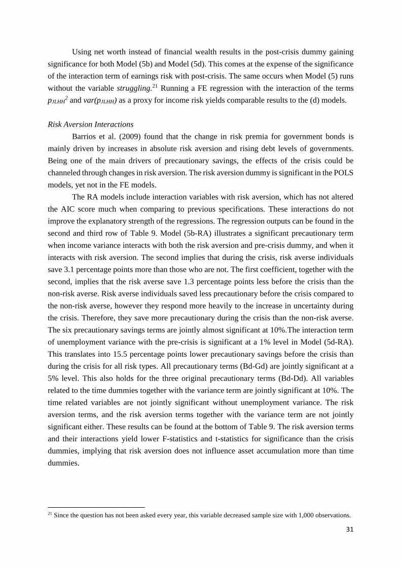
31

Using net worth instead of financial wealth results in the post-crisis dummy gaining

significance for both Model (5b) and Model (5d). This comes at the expense of the significance

of the interaction term of earnings risk with post-crisis. The same occurs when Model (5) runs

without the variable struggling.21 Running a FE regression with the interaction of the terms

pJLHH2 and var(pJLHH) as a proxy for income risk yields comparable results to the (d) models.

Risk Aversion Interactions

Barrios et al. (2009) found that the change in risk premia for government bonds is

mainly driven by increases in absolute risk aversion and rising debt levels of governments.

Being one of the main drivers of precautionary savings, the effects of the crisis could be

channeled through changes in risk aversion. The risk aversion dummy is significant in the POLS

models, yet not in the FE models.

The RA models include interaction variables with risk aversion, which has not altered

the AIC score much when comparing to previous specifications. These interactions do not

improve the explanatory strength of the regressions. The regression outputs can be found in the

second and third row of Table 9. Model (5b-RA) illustrates a significant precautionary term

when income variance interacts with both the risk aversion and pre-crisis dummy, and when it

interacts with risk aversion. The second implies that during the crisis, risk averse individuals

save 3.1 percentage points more than those who are not. The first coefficient, together with the

second, implies that the risk averse save 1.3 percentage points less before the crisis than the

non-risk averse. Risk averse individuals saved less precautionary before the crisis compared to

the non-risk averse, however they respond more heavily to the increase in uncertainty during

the crisis. Therefore, they save more precautionary during the crisis than the non-risk averse.

The six precautionary savings terms are jointly almost significant at 10%.The interaction term

of unemployment variance with the pre-crisis is significant at a 1% level in Model (5d-RA).

This translates into 15.5 percentage points lower precautionary savings before the crisis than

during the crisis for all risk types. All precautionary terms (Bd-Gd) are jointly significant at a

5% level. This also holds for the three original precautionary terms (Bd-Dd). All variables

related to the time dummies together with the variance term are jointly significant at 10%. The

time related variables are not jointly significant without unemployment variance. The risk

aversion terms, and the risk aversion terms together with the variance term are not jointly

significant either. These results can be found at the bottom of Table 9. The risk aversion terms

and their interactions yield lower F-statistics and t-statistics for significance than the crisis

dummies, implying that risk aversion does not influence asset accumulation more than time

dummies.

21 Since the question has not been asked every year, this variable decreased sample size with 1,000 observations.

32

Table 9. Risk aversion interaction, Sensitivity 1 & 2, LN(Ait/Yit), both proxies, FE, robust errors.

# VARIABLES 5b-RA 5d-RA 5b-S1 5b -S2

A LN(Yit) -0.453*** -0.430*** -0.382*** -0.444***

(0.0719) (0.0688) (0.116) (0.0836)

B σ2y/Yit -1.89e-05 -5.38e-05 7.69e-05**

(3.39e-05) (3.50e-05) (3.31e-05)

C σ2/Yit *Pre 3.88e-05 0.000133*** -5.94e-05

(4.70e-05) (4.50e-05) (4.55e-05)

D σ2/Yit *Post -5.56e-05 -0.000100*** -0.000130

(4.41e-05) (3.57e-05) (0.000163)

E σ2/Yit *Pre*ϴ -0.000121*

(6.24e-05)

F σ2/Yit *Post*ϴ -0.000130

(0.000146)

G σ2/Yit *ϴ 8.68e-05*

(4.49e-05)

Bd Var(PJLHH)it 0.345

(0.377)

Cd Var(PJLHH)it*Pre -1.641***

(0.607)

Dd Var(PJLHH)it*Post 0.909

(1.467)

Ed Var(PJLHH)it*Pre*ϴ -1.054

(1.670)

Fd Var(PJLHH)it*Post *ϴ 0.688

(0.770)

Gd Var(PJLHH)it *ϴ -0.432

(0.435)

H Pre*ϴ 0.0319 0.345

(0.0803) (0.106)

I Post*ϴ -0.00308 0.0310

(0.125) (0.173)

J ϴ -0.0170 0.0541 0.0376 -0.0204

(0.0509) (0.0644) (0.0511) (0.0630)

K Pre-crisis 0.000315 0.172* -0.0356 0.0757

(0.0861) (0.0995) (0.0729) (0.0785)

L Post-crisis 0.0871 0.0150 0.151* 0.0782

(0.117) (0.151) (0.0865) (0.0867)

Age 0.0868 0.0696 0.168 0.0139

(0.170) (0.167) (0.226) (0.208)

Age2 -0.00178 -0.00147 -0.00457 0.000197

(0.00370) (0.00364) (0.00485) (0.00459)

Age3/102 0.00140 0.00125 0.00386 -6.58e-05

(0.00261) (0.00258) (0.00340) (0.00329)

Family Size -0.103 -0.0747 -0.0901 0.0458

(0.145) (0.141) (0.202) (0.125)

Children 0.204 0.164 0.303 -0.00499

(0.190) (0.183) (0.260) (0.119)

Self-employed -0.0378 -0.0301 -0.116 -0.00353

(0.136) (0.130) (0.138) (0.219)

Public-sector -0.0397 -0.0253 0.148 0.0676

(0.0908) (0.0883) (0.129) (0.110)

Cohort Dummies Yes Yes Yes Yes

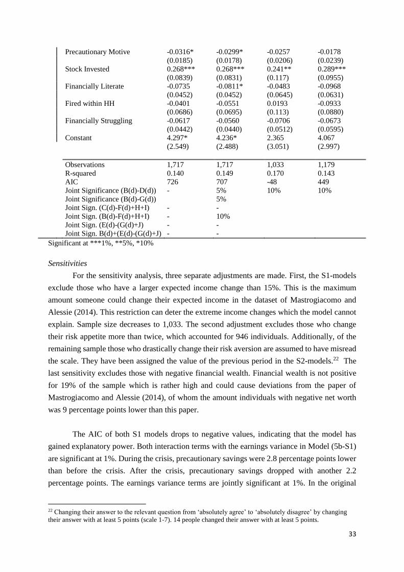
33

Precautionary Motive -0.0316* -0.0299* -0.0257 -0.0178

(0.0185) (0.0178) (0.0206) (0.0239)

Stock Invested 0.268*** 0.268*** 0.241** 0.289***

(0.0839) (0.0831) (0.117) (0.0955)

Financially Literate -0.0735 -0.0811* -0.0483 -0.0968

(0.0452) (0.0452) (0.0645) (0.0631)

Fired within HH -0.0401 -0.0551 0.0193 -0.0933

(0.0686) (0.0695) (0.113) (0.0880)

Financially Struggling -0.0617 -0.0560 -0.0706 -0.0673

(0.0442) (0.0440) (0.0512) (0.0595)

Constant 4.297* 4.236* 2.365 4.067

(2.549) (2.488) (3.051) (2.997)

Observations 1,717 1,717 1,033 1,179

R-squared 0.140 0.149 0.170 0.143

AIC 726 707 -48 449

Joint Significance (B(d)-D(d))

Joint Significance (B(d)-G(d))

Joint Sign. (C(d)-F(d)+H+I)

Joint Sign. (B(d)-F(d)+H+I)

Joint Sign. (E(d)-(G(d)+J)

Joint Sign. B(d)+(E(d)-(G(d)+J)

-

-

-

-

-

5%

5%

-

10%

-

-

10%

10%

Significant at ***1%, **5%, *10%

Sensitivities

For the sensitivity analysis, three separate adjustments are made. First, the S1-models

exclude those who have a larger expected income change than 15%. This is the maximum

amount someone could change their expected income in the dataset of Mastrogiacomo and

Alessie (2014). This restriction can deter the extreme income changes which the model cannot

explain. Sample size decreases to 1,033. The second adjustment excludes those who change

their risk appetite more than twice, which accounted for 946 individuals. Additionally, of the

remaining sample those who drastically change their risk aversion are assumed to have misread

the scale. They have been assigned the value of the previous period in the S2-models.22 The

last sensitivity excludes those with negative financial wealth. Financial wealth is not positive

for 19% of the sample which is rather high and could cause deviations from the paper of

Mastrogiacomo and Alessie (2014), of whom the amount individuals with negative net worth

was 9 percentage points lower than this paper.

The AIC of both S1 models drops to negative values, indicating that the model has

gained explanatory power. Both interaction terms with the earnings variance in Model (5b-S1)

are significant at 1%. During the crisis, precautionary savings were 2.8 percentage points lower

than before the crisis. After the crisis, precautionary savings dropped with another 2.2

percentage points. The earnings variance terms are jointly significant at 1%. In the original

22 Changing their answer to the relevant question from ‘absolutely agree’ to ‘absolutely disagree’ by changing

their answer with at least 5 points (scale 1-7). 14 people changed their answer with at least 5 points.

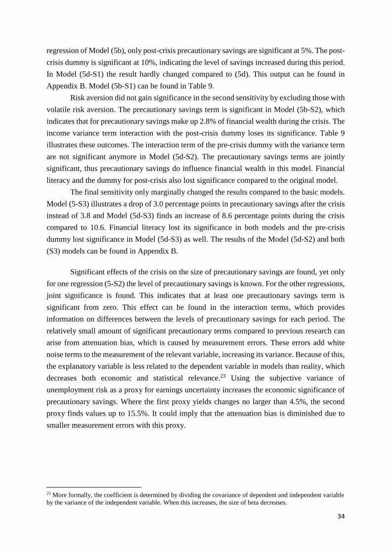
34

regression of Model (5b), only post-crisis precautionary savings are significant at 5%. The post-

crisis dummy is significant at 10%, indicating the level of savings increased during this period.

In Model (5d-S1) the result hardly changed compared to (5d). This output can be found in

Appendix B. Model (5b-S1) can be found in Table 9.

Risk aversion did not gain significance in the second sensitivity by excluding those with

volatile risk aversion. The precautionary savings term is significant in Model (5b-S2), which

indicates that for precautionary savings make up 2.8% of financial wealth during the crisis. The

income variance term interaction with the post-crisis dummy loses its significance. Table 9

illustrates these outcomes. The interaction term of the pre-crisis dummy with the variance term

are not significant anymore in Model (5d-S2). The precautionary savings terms are jointly

significant, thus precautionary savings do influence financial wealth in this model. Financial

literacy and the dummy for post-crisis also lost significance compared to the original model.

The final sensitivity only marginally changed the results compared to the basic models.

Model (5-S3) illustrates a drop of 3.0 percentage points in precautionary savings after the crisis

instead of 3.8 and Model (5d-S3) finds an increase of 8.6 percentage points during the crisis

compared to 10.6. Financial literacy lost its significance in both models and the pre-crisis

dummy lost significance in Model (5d-S3) as well. The results of the Model (5d-S2) and both

(S3) models can be found in Appendix B.

Significant effects of the crisis on the size of precautionary savings are found, yet only

for one regression (5-S2) the level of precautionary savings is known. For the other regressions,

joint significance is found. This indicates that at least one precautionary savings term is

significant from zero. This effect can be found in the interaction terms, which provides

information on differences between the levels of precautionary savings for each period. The

relatively small amount of significant precautionary terms compared to previous research can

arise from attenuation bias, which is caused by measurement errors. These errors add white

noise terms to the measurement of the relevant variable, increasing its variance. Because of this,

the explanatory variable is less related to the dependent variable in models than reality, which

decreases both economic and statistical relevance.23 Using the subjective variance of

unemployment risk as a proxy for earnings uncertainty increases the economic significance of

precautionary savings. Where the first proxy yields changes no larger than 4.5%, the second

proxy finds values up to 15.5%. It could imply that the attenuation bias is diminished due to

smaller measurement errors with this proxy.

23 More formally, the coefficient is determined by dividing the covariance of dependent and independent variable

by the variance of the independent variable. When this increases, the size of beta decreases.

35

6. Conclusion and Policy Recommendations

Previous research into precautionary savings has shown that its economic relevance

varies per country and estimation method of income uncertainty. When subjective measures are

used, economic relevance is generally smaller with precautionary savings making up about 4%

of savings (Kennickell and Lusardi, 2004). Using objective measures, the size increases to 30%

(Mastrogiacomo and Alessie, 2014). Using the appropriate proxy for income uncertainty, in

their case eligibility to unemployment benefits, and aggregating risk on household level, the

objective and subjective measure provide comparable outcomes. This paper uses the subjective

earnings risk reported by Dutch households during 2004-2016 as the initial measure of income

risk to estimate the effect of the crisis on precautionary savings. As an alternative, the variance

of unemployment risk on household level was used.

This paper finds that the measure of subjective income variance yields lower statistically

and economically significant results than the proxy regarding unemployment risk.

Approximations of the exact level of precautionary savings could only be found in one model

for the level of during the crisis, which equaled 2.7% of financial wealth. This is a rather

economically insignificant result. However, the effects of the crisis on the level of precautionary

savings yielded larger differences of a higher level, reaching up to a 15% difference between

precautionary savings before and during the crisis. This is achieved when the proxy for earning

uncertainty is variance of unemployment risk. The other proxy, income variance, yielded the

result of lower precautionary savings after the crisis of about 3% compared to during the crisis.

When the risk aversion type was accounted for, one finds that before the crisis, risk averse

individuals save less precautionary than the non-risk averse. However, during the crisis risk

averse individuals exhibited more precautionary savings than the non-risk averse. A possible

explanation of non-risk averse people having more precautionary savings before the crisis is

that risk averse saved more regardless of income risks before the crisis, which lowers the need

for an additional buffer against income risks. Yet when the crisis started, the risk averse

individuals responded more heavily to the increase in uncertainty than the non-risk averse. The

risk averse insignificantly show higher savings in the period before the crisis.

The proxy of unemployment risk increases the significance of the models and is deemed

to be a suitable alternative measure of income uncertainty. Exogeneity of the original proxy of

income uncertainty, earnings variance, cannot be rejected. As a result, an IV has not been

implemented, as opposed to comparable papers. This paper’s insignificant precautionary

savings terms, when the identical initial regression of Mastrogiacomo and Alessie (2014) is

performed, do suggest that the measure of earnings variance in this paper might suffer from

measurement errors. Especially since the model’s explanatory power increased when only the

reasonable ranges for income changes were included in the regressions.

36

Risk aversion hardly influenced one’s level of financial wealth, and only has significant

influences when it interacts with the uncertainty proxies. The other controls proposed in this

paper increased explanatory power of the models, and thus reducing the problem of omitted

variable bias. Precautionary terms were only significant when these controls were added.

Investing in stocks is an important variable for the model, being strongly positively significant

in all models. Financial literacy has proven to be significant in multiple model specifications,

however a peculiar negative sign is found. This could also be caused by generally higher

savings.

Based on the results in this paper, it can be concluded that during the crisis the Dutch

population exhibited more precautionary behavior in terms of higher savings than in periods

before and after the crisis. This is in line with the finding of Broadway and Halsken (2017),

however they find that precautionary savings overshoot during the Great Recession. The higher

level of precautionary savings during the crisis does not necessarily prove overshooting for this

data set. When uncertainty increases, the rational response of a prudent agent is to increase

savings, yet if there is overshooting in savings, this is a suboptimal outcome from a welfare

perspective. When overshooting occurs, the government should tackle this inefficiency. Also,

when one cannot speak of overshooting a drop in consumption during economic downturn

amplifies the problem of a decelerating economy. In order to stimulate the economy,

governments could provide additional security to employees to overcome subjective income

uncertainty. Putting more restrictions in place to complicate firing employees during economic

downturn hurts employers. Increased unemployment benefits during economic downturn could

provide a solution, yet one must be weary of moral hazard if doing so. Employees would not

be incentivized to search for a new job if these benefits are too high.

For future research on precautionary savings, using the variance of unemployment risk

as proxy for earnings uncertainty, offers great possibilities. This variable seems to suffer less

from measurement errors and focuses on the main earnings uncertainty employees face, which

is unemployment. The other proxy for earnings uncertainty, earnings variance, yields more

favorable results when restricted to sensible ranges of income changes, and these restrictions

are advised to implement in future research as well. Real income changes are what really drives

agents, thus better results could be obtained when inflation rates are included, especially when

inflation rates rise again. By including more post-crisis years in future papers, the difference

between the crisis and the post-crisis period can be evaluated better, because this paper only

has information on two years of post-crisis circumstances. This inclusion of more observations

could improve the economic and statistical significance of comparable models. Also, research

into the differences in precautionary savings for those who invest in stocks, and those who are

financially literate would be an interesting expansion of current literature. These variables have

shown to significantly influence the level of assets and due to this difference in financial buffer

could exhibit different precautionary behavior.

37

Reference list

Alan, S., Crossley, T., Low, H., 2012. Saving on a rainy day, borrowing for a rainy day,

Unpublished working paper. Koc University.

Alessie, R., Lusardi, A., 1997. Consumption, savings, and habit formation. Economics Letters

55, 103-108.

Barrios, S., Iversen, P., Lewandowska, M., Setzer, R., 2009. Determinants of intra-euro area

government bond spreads during the financial crisis," European Economy. Economic Papers

388.

Broadway, B., Halsken- DeNew, J.P., 2017. Keep calm and consume? Subjective uncertainty

and precautionary savings. Unpublished working paper. Melbourne Institute Working Paper

18.

Caballero, R.J., 1989. Consumption puzzle and precautionary savings. Journal of Monetary

Economics 25, 113-136.

Carroll, C.D., Hall, R.E., Zeldes, S.P., 1992. The buffer-stock theory of saving. Brookings

Papers on Economic Activity 2, 61-156.

Carroll, C.D., Samwick, A.A., 1998. How important is precautionary savings? The Review of

Economics and Statistics, 80-3, 410-419.

Carroll, C.D., Slacalek, J., Sommer, M., 2012. Dissecting saving dynamics: Measuring wealth,

precautionary, and credit effects. Unpublished working paper. ECB Working Paper 1474.

Collins, J.M., 2012. Financial advice: A substitute for financial literacy? Financial Services

Review 21.

Dominitz, J., Manski, C.F., 1997. Using expectations data to study subjective income

expectations. Journal of the American Statistical Association, 92- 439, 855-867.

Fisher, I., 1930. The theory of interest, as determined by impatience to spend income and

opportunity to invest it. Macmillan, New York.

Friedman, M., 1957. A Theory of the Consumption Function. Princeton University

Press, New Jersey, pp. 20- 37.

38

Gourinchas P.O., Parker, J.A., 2003. Consumption over the lifecycle. Econometrica 70-1, 47-

89.

Guiso, L., Jappelli, T., Terlizzese, D., 1992. Earnings uncertainty and precautionary saving.

Journal of Monetary Economics 30 , 307- 337.

Heaton, J., Lucas, D., 1997. Market frictions, savings behavior, and portfolio choice.

Macroeconomic Dynamics 1-1, 76 – 101.

Hochguertel, S., 2003. Precautionary motives and portfolio decisions. Journal of Applied

Econometrics 18, 61-77.

Jappelli, T., Padula, M., Pistaferri, L., 2008. A direct test of the buffer-stock model of saving.

Journal of European Economic Association 6-6, 1186-1210.

Kahneman, D., Tversky, A., 1979. Prospect Theory: An analysis of decision under risk.

Econometrica 47-2, 263-292.

Kennickell, A., Lusardi, A., 2004. Disentangling the importance of the precautionary saving

motive. Unpublished working paper. CFS Working Paper 15.

Keynes, J. M., (1936). The general theory of employment, interest and money. New York:

Harcourt Brace Jovanovich.

Kimball, M.S., 1990-a. Precautionary saving in the small and in the large. Econometrica 58-1,

53-73.

Kimball, M.S., 1990-b. Precautionary saving and the marginal propensity to consume.

Unpublished Working Paper. NBER Working Paper 3403.

Maki, D.M., Palumbo, M.G., 2001. Disentangling the wealth effect: A cohort analysis of

household saving in the 1990s. Unpublished working paper. FEDS Working Paper 21.

Mastrogiacomo, M., Alessie, R., 2011. Did you really save so little for your retirement? An

analysis of retirement savings and unconventional retirement accounts. Netspar Discussion

Paper 12.

39

Mastrogiacomo, M., Alessie, R., 2014. The precautionary savings motive and household

savings. Oxford Economic Papers- New Series 66-1, 164-187.

Mody. A., Ohnsorge, F., Sandri, D., 2012. Precautionary savings in the Great Recession. IMF

Economic Review, 60-1, 114-138.

Naranjo, D.V., Van Gameren, E., 2016. Precautionary savings in Mexico: Evidence form the

Mexican health and aging study. Review of Income and Wealth 62-2, 334-361.

Paiella, M. , 2007. Does wealth affect consumption? Evidence for Italy. Journal of

Macroeconomics 29, 189- 205.

Rossi, M., Sansone, D., 2016. Precautionary savings and the self-employed: Does uncertainty

magnitude matter. Netspar Discussing Paper 7.

Watson, J.J., 2003.The relationship of materialism to spending tendencies, saving, and debt.

Journal of Economic Psychology 24, 723-739.

Weil, P., 1993. Precautionary savings and the permanent income hypothesis. Review of

Economic Studies 60, 367-383.

Zandi, M.P., 1999. “Wealth worries”. Regional Financial Review Aug, 1-8.

Appendix

40

Appendix A: Variables

Definitions:

Financial wealth: Sum of current assets and current liabilities

Net worth: Sum of financial assets, illiquid assets and mortgages.

Current assets: Savings, deposits, saving certificates, growth funds, mutual funds, bonds,

shares, money lend out, other investments, life-course savings and savings at the employer. If

checking-accounts are positive they are added.

Current liabilities: Personal loans, credit lines, other loans, remaining loans, loans from the

family, study loans, credit cards, other debt and arrears. If checking-accounts are negative they

are added as well.

Illiquid assets: Real-estate, cars, motorcycles, boats, campers, annuity insurance and

endowment insurance.

Construction:

Example of value ranges offered to respondents. For all values except 15, the value of assets

was determined as the average of the value range. For 15, the asset/liability was given the lower

bound.

“Into which of the categories mentioned below did the remaining debt go?

1 less than € 50 .......................................................................................FAMI1

2 € 50 to € 250 ........................................................................................FAMI1

3 € 250 to € 500 ......................................................................................FAMI1

4 € 500 to € 750 ......................................................................................FAMI1

5 € 750 to € 1.000 ...................................................................................FAMI1

6 € 1.000 to € 2.500 ................................................................................FAMI1

7 € 2.500 to € 5.000 ................................................................................FAMI1

8 € 5.000 to € 7.500 ................................................................................FAMI1

9 € 7.500 to € 10.000 ..............................................................................FAMI1

10 € 10.000 to € 11.500 ..........................................................................FAMI1

11 € 11.500 to € 14.000 ..........................................................................FAMI1

12 € 14.000 to € 17.000 ..........................................................................FAMI1

13 € 17.000 to € 20.000 ..........................................................................FAMI1

14 € 20.000 to € 25.000 ..........................................................................FAMI1

15 € 25.000 or more ................................................................................FAMI1

-9 don’t know ..........................................................................................FAMI1”

Changes in survey:

• Savings earned at employer has been adjusted.

41

• Number of loans on estate have been decreased.

• Growth fund has been deleted from the survey since 2008.

• Life course something added in the survey 2007

Creation of variables:

Working:

Respondents gave contradicting answers regarding occupation. The question which asks

specifically about primary occupation was used as the leading variable, yet if at least one

question would suggest employment, the person is classified as part of the working population.

Education: Special education added to other education, since this group was very small. No one

of the heads has no education. All the high school groups have been merged into one group as

well.

Risk Aversion:

“I think it is more important to have safe investments and guaranteed returns, than to take a

risk to have a chance to get the highest possible returns.”

Answer the following question, where a score of at least 5 out of 7 would classify

someone as ‘Risk averse’

Motivation for precautionary savings:

“To save to have some savings to cover unforeseen expenses” Used as a scale variable.

Struggling financially24:

“if necessary, we/I can reduce our/my household’s expenditures by 5% without a problem”

Answer the following question, where a score of at least 5 out of 7 would classify

someone as ‘Struggling’

Head of household:

“BESLIS Which of the following four statements would best describe the way in which financial

matters are decided in your household?

1 I leave it to my partner to decide on financial matters .............................................. GELDH

2 My partner has more influence than me on financial decisions ................................ GELDH

3 My partner and I have equal influence on financial decisions .................................. GELDH

4 I have more influence on financial decisions than my partner does ......................... GELDH

5 My partner leaves the financial decisions to me… .................................................. GELDH”

When one spouse answers 1/2/3 and the other 4/5, the one with the 4/5 score is

considered the head. If this yields no dominance, it is the person registered as head of household.

24 The relevant question is not asked during the surveys of 2008, 2010, 2012. 2014 and 2016

42

Appendix B: Regressions

Table B.1 IV regression, on LN(Ait/Yit), White Errors. Proxy : σ2y/Yit, IVs: var(pJLHH) & pJLHH

2

VARIABLES 2c 3c 4c 5c

σ2y/Yit -0.000294 -5.24e-05 -0.000198 0.000367

(0.000224) (0.000232) (0.000287) (0.000273)

σ2/Yit *Pre -0.00194 0.000642 -0.000232

(0.00198) (0.00259) (0.000740)

σ2/Yit *Post -2.96e-05 -0.000293 -0.00247

(0.00128) (0.00151) (0.00293)

LN(Yit) 0.157 0.371 0.0359 -0.0335

(0.119) (0.293) (0.328) (0.189)

ϴ 0.0855 0.159**

(0.110) (0.0697)

Age 0.223** 0.353 0.249 0.221

(0.113) (0.231) (0.266) (0.181)

Age2 -0.00438* -0.00757 -0.00463 -0.00405

(0.00258) (0.00540) (0.00581) (0.00399)

Age3/102 0.00295 0.00538 0.00289 0.00240

(0.00190) (0.00399) (0.00442) (0.00287)

Family Size -0.0570 -0.128 -0.0308 -0.306**

(0.0621) (0.133) (0.113) (0.119)

Children 0.00972 0.0624 -0.00652 0.227*

(0.0759) (0.129) (0.108) (0.133)

Self-employed 0.133 0.173

(0.479) (0.302)

Pre-crisis 0.882 -0.154 0.133

(0.788) (0.986) (0.281)

Post-crisis -0.0800 0.108 0.758

(0.518) (0.615) (0.826)

Public-sector 0.189 0.140*

(0.208) (0.0753)

Cohort Dummies Yes Yes

Precautionary Motive 0.0307 -0.0648

(0.0555) (0.0553)

Stock Invested 0.382***

(0.102)

Financially Literate 0.128**

(0.0596)

Fired within HH 0.0235

(0.0862)

Financially Struggling -0.215***

(0.0589)

Constant -4.769** -8.572 -4.494 -2.883

(2.010) (5.254) (4.517) (3.160)

Observations 3,012 3,012 3,012 1,717

Sargan (p-value)ˁ 0.019(0.89) 0.827(0.84) 5.657(0.13) 2.846(0.42)

Validity (F-Stat) ˁ 5.03 5.27 5.97 4.52

Exogeneity° (p-value) 1.642(0.20) 0.913(0.43) 0.308(0.82) 2.055(0.10)

°σ2y/Yit, ˁVar(PJLHH) + (PJLHH)2 . Significant at ***1%, **5%, *10%

43

Table B.2. FE regression, LN(Ait/Yit) White Errors, sample size equal to proxy var(pJL). Proxy: σ2y/Yit

VARIABLES 2b 3b 4b 5b

LN(Yit) -0.406*** -0.409*** -0.411*** -0.450***

(0.0471) (0.0479) (0.0477) (0.0721)

σ2y/Yit 2.83e-06 1.77e-05 1.83e-05 4.03e-05

(1.07e-05) (1.64e-05) (1.65e-05) (3.07e-05)

σ2/Yit *Pre -2.89e-05 -2.94e-05 -4.35e-05

(2.00e-05) (1.99e-05) (3.45e-05)

σ2/Yit *Post -2.16e-05 -2.16e-05 -0.000101**

(2.65e-05) (2.60e-05) (4.43e-05)

ϴ -0.0208 -0.000249

(0.0283) (0.0411)

Age 0.172 0.171 0.208 0.0796

(0.147) (0.147) (0.153) (0.167)

Age2 -0.00333 -0.00343 -0.00422 -0.00163

(0.00317) (0.00315) (0.00328) (0.00363)

Age3/102 0.00225 0.00234 0.00288 0.00130

(0.00221) (0.00220) (0.00228) (0.00256)

Family Size 0.0179 0.0133 0.0122 -0.0999

(0.0654) (0.0646) (0.0637) (0.145)

Children 0.0639 0.0689 0.0681 0.190

(0.0954) (0.0954) (0.0942) (0.190)

Self-employed -0.0220 -0.0400

(0.0719) (0.136)

Pre-crisis 0.0134 0.00452 0.0205

(0.0417) (0.0432) (0.0596)

Post-crisis 0.0878** 0.0826* 0.0748

(0.0445) (0.0445) (0.0669)

Public-sector 0.0622 -0.0262

(0.0498) (0.0899)

Cohort Dummies Yes Yes

Precautionary Motive -0.0171 -0.0334*

(0.0112) (0.0185)

Stock Invested 0.263***

(0.0838)

Financially Literate -0.0778*

(0.0453)

Fired within HH -0.0464

(0.0688)

Financially Struggling -0.0601

(0.0439)

Constant 1.522 1.692 1.357 4.405*

(2.191) (2.211) (2.318) (2.501)

Observations 3,012 3,012 3,012 1,717

R-squared 0.099 0.103 0.107 0.136

AIC 1,477 1,472 1,473 726

F-test: u0 =0 7.68 7.64 7.53 4.57

Joint Significance - - - 5%

Significant at ***1%, **5%, *10%

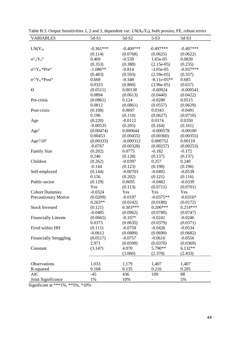
44

Table B.3. Output Sensitivities 1, 2 and 3, dependent var: LN(Ait/Yit), both proxies, FE, robust errors

VARIABLES 5d-S1 5d-S2 5-S3 5d-S3

LN(Yit) -0.361*** -0.400*** -0.497***

-0.497***

(0.114) (0.0768) (0.0625) (0.0622)

σ2y/Yit° 0.469 -0.539 1.65e-05 0.0830

(0.353) (0.388) (2.15e-05) (0.235)

σ2/Yit *Pre° -1.086** -0.814 -3.05e-05 -0.937***

(0.483) (0.593) (2.59e-05) (0.357)

σ2/Yit *Post° 0.669 -0.348 -8.11e-05** 0.685

0.0323 (0.860) (3.96e-05) (0.637)

ϴ (0.0511) 0.00138 -0.00924 -0.000541

0.0894 (0.0613) (0.0440) (0.0422)

Pre-crisis (0.0861) 0.124 -0.0280 0.0515

0.0812 (0.0861) (0.0557) (0.0629)

Post-crisis (0.108) 0.0697 0.0343 -0.0491

0.196 (0.110) (0.0627) (0.0710)

Age (0.220) -0.0112 0.0174 0.0350

-0.00535 (0.205) (0.164) (0.161)

Age2 (0.00474) 0.000644 -0.000578 -0.00100

0.00453 (0.00455) (0.00360) (0.00355)

Age3/102 (0.00333) -0.000312 0.000752 0.00110

-0.0767 (0.00328) (0.00257) (0.00253)

Family Size (0.202) 0.0775 -0.182 -0.172

0.246 (0.128) (0.137) (0.137)

Children (0.262) -0.0397 0.257 0.240

-0.144 (0.123) (0.198) (0.196)

Self-employed (0.144) -0.00703 -0.0492 -0.0538

0.156 (0.202) (0.121) (0.116)

Public-sector (0.129) 0.0695 -0.0482 -0.0339

Yes (0.113) (0.0711) (0.0701)

Cohort Dummies -0.0324 Yes Yes Yes

Precautionary Motive (0.0209) -0.0197 -0.0375** -0.0316*

0.263** (0.0242) (0.0180) (0.0172)

Stock Invested (0.121) 0.303*** 0.206*** 0.214***

-0.0485 (0.0962) (0.0780) (0.0747)

Financially Literate (0.0665) -0.107* -0.0241 -0.0246

0.0373 (0.0635) (0.0379) (0.0371)

Fired within HH (0.111) -0.0759 -0.0426 -0.0534

-0.0612 (0.0889) (0.0690) (0.0682)

Financially Struggling (0.0517) -0.0757 -0.0610 -0.0556

2.971 (0.0599) (0.0370) (0.0369)

Constant (3.147) 4.070 5.790** 6.132**

(3.060) (2.370) (2.433)

Observations 1,033 1,179 1,407 1,407

R-squared 0.168 0.135 0.216 0.205

AIC -45 436 109 88

Joint Significance 1% 10% - 5%

Significant at ***1%, **5%, *10%

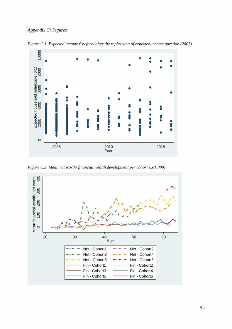
45

Appendix C: Figures

Figure C.1. Expected income € before/ after the rephrasing of expected income question (2007)

Figure C.2. Mean net worth/ financial wealth development per cohort (x€1,000)

010

020

030

040

0M

ean

finan

cial

wea

lth/ n

et w

orth

20 30 40 50 60Age

Net - Cohort1 Net - Cohort2Net - Cohort3 Net - Cohort4Net - Cohort5 Net - Cohort6Fin - Cohort1 Fin - Cohort2Fin - Cohort3 Fin - Cohort4Fin - Cohort5 Fin - Cohort6

020

004

000

6000

8000

1000

0E

xpec

ted

hou

seho

ld n

etin

com

e (t

+1)

2005 2010 2015Year