Swarthmore College Swarthmore College

Works Works

Physics & Astronomy Faculty Works Physics & Astronomy

4-1-2021

Precise Transit And Radial-Velocity Characterization Of A Precise Transit And Radial-Velocity Characterization Of A

Resonant Pair: The Warm Jupiter TOI-216c And Eccentric Warm Resonant Pair: The Warm Jupiter TOI-216c And Eccentric Warm

Neptune TOI-216b Neptune TOI-216b

R. I. Dawson

C. X. Huang

R. Brahm

K. A. Collins

M. J. Hobson

See next page for additional authors

Follow this and additional works at: https://works.swarthmore.edu/fac-physics

Part of the Astrophysics and Astronomy Commons

Let us know how access to these works benefits you

Recommended Citation Recommended Citation R. I. Dawson, C. X. Huang, R. Brahm, K. A. Collins, M. J. Hobson, A. Jordán, J. Dong, J. Korth, T. Trifonov, L. Abe, A. Agabi, I. Bruni, R. P. Butler, M. Barbieri, K. I. Collins, D. M. Conti, J. D. Crane, N. Crouzet, G. Dransfield, P. Evans, N. Espinoza, T. Gan, T. Guillot, T. Henning, J. J. Lissauer, Eric L. N. Jensen, W. M. Sainte, D. Mékarnia, G. Myers, S. Nandakumar, H. M. Relles, P. Sarkis, P. Torres, S. Shectman, F.-X. Schmider, A. Shporer, C. Stockdale, J. Teske, A. H. M. J. Triaud, S. X. Wang, C. Ziegler, G. Ricker, R. Vanderspek, D. W. Latham, S. Seager, J. Winn, J. M. Jenkins, L. G. Bouma, J. A. Burt, D. Charbonneau, A. M. Levine, S. McDermott, B. McLean, M. E. Rose, A. Vanderburg, and B. Wohler. (2021). "Precise Transit And Radial-Velocity Characterization Of A Resonant Pair: The Warm Jupiter TOI-216c And Eccentric Warm Neptune TOI-216b". The Astronomical Journal. Volume 161, Issue 4. DOI: 10.3847/1538-3881/abd8d0 https://works.swarthmore.edu/fac-physics/425

This work is brought to you for free by Swarthmore College Libraries' Works. It has been accepted for inclusion in Physics & Astronomy Faculty Works by an authorized administrator of Works. For more information, please contact myworks@swarthmore.edu.

Authors Authors R. I. Dawson, C. X. Huang, R. Brahm, K. A. Collins, M. J. Hobson, A. Jordán, J. Dong, J. Korth, T. Trifonov, L. Abe, A. Agabi, I. Bruni, R. P. Butler, M. Barbieri, K. I. Collins, D. M. Conti, J. D. Crane, N. Crouzet, G. Dransfield, P. Evans, N. Espinoza, T. Gan, T. Guillot, T. Henning, J. J. Lissauer, Eric L. N. Jensen, W. M. Sainte, D. Mékarnia, G. Myers, S. Nandakumar, H. M. Relles, P. Sarkis, P. Torres, S. Shectman, F.-X. Schmider, A. Shporer, C. Stockdale, J. Teske, A. H. M. J. Triaud, S. X. Wang, C. Ziegler, G. Ricker, R. Vanderspek, D. W. Latham, S. Seager, J. Winn, J. M. Jenkins, L. G. Bouma, J. A. Burt, D. Charbonneau, A. M. Levine, S. McDermott, B. McLean, M. E. Rose, A. Vanderburg, and B. Wohler

This article is available at Works: https://works.swarthmore.edu/fac-physics/425

Precise Transit and Radial-velocity Characterization of a Resonant Pair: The WarmJupiter TOI-216c and Eccentric Warm Neptune TOI-216b

Rebekah I. Dawson1 , Chelsea X. Huang2,36 , Rafael Brahm3,4 , Karen A. Collins5 , Melissa J. Hobson4,6 ,Andrés Jordán3,4, Jiayin Dong1,7 , Judith Korth8, Trifon Trifonov9 , Lyu Abe10, Abdelkrim Agabi10, Ivan Bruni11,

R. Paul Butler12 , Mauro Barbieri13 , Kevin I. Collins14 , Dennis M. Conti15 , Jeffrey D. Crane16 , Nicolas Crouzet17 ,Georgina Dransfield18, Phil Evans19, Néstor Espinoza20 , Tianjun Gan21 , Tristan Guillot10 , Thomas Henning9 ,

Jack J. Lissauer22, Eric L. N. Jensen23 , Wenceslas Marie Sainte24, Djamel Mékarnia10 , Gordon Myers25 ,Sangeetha Nandakumar13, Howard M. Relles5, Paula Sarkis9 , Pascal Torres4,6, Stephen Shectman16 ,

François-Xavier Schmider10 , Avi Shporer2 , Chris Stockdale26 , Johanna Teske16,37, Amaury H. M. J. Triaud18 ,Sharon Xuesong Wang16, Carl Ziegler27 , G. Ricker2 , R. Vanderspek2 , David W. Latham5 , S. Seager2,28,29, J. Winn30 ,

Jon M. Jenkins22 , L. G. Bouma30 , Jennifer A. Burt31 , David Charbonneau5 , Alan M. Levine2, Scott McDermott32,Brian McLean33 , Mark E. Rose22 , Andrew Vanderburg34,38 , and Bill Wohler22,35

1 Department of Astronomy & Astrophysics, Center for Exoplanets and Habitable Worlds, The Pennsylvania State University, University Park, PA 16802, USArdawson@psu.edu

2 Department of Physics and Kavli Institute for Astrophysics and Space Research, Massachusetts Institute of Technology, Cambridge, MA 02139, USA3 Facultad de Ingeniería y Ciencias, Universidad Adolfo Ibáñez, Av. Diagonal las Torres 2640, Peñalolén, Santiago, Chile

4 Millennium Institute for Astrophysics, Chile5 Harvard-Smithsonian Center for Astrophysics, 60 Garden Street, Cambridge, MA 02138, USA

6 Instituto de Astrofísica, Facultad de Física, Pontificia Universidad Católica de Chile, Chile7 Center for Computational Astrophysics, Flatiron Institute, 162 Fifth Avenue, New York, NY 10010, USA

8 Rheinisches Institut für Umweltforschung, Abteilung Planetenforschung an der Universität zu Köln, Universität zu Köln, Aachenerstraße 209, D-50931 Köln,Germany

9 Max Planck Institute for Astronomy, Koenigstuhl 17, D-69117 Heidelberg, Germany10 Université Côte d’Azur, Observatoire de la Côte d’Azur, CNRS, Laboratoire Lagrange Bd de l’Observatoire, CS 34229, F-06304 Nice Cedex 4, France

11 INAF OAS, Osservatorio di Astrofisica e Scienza dello Spazio di Bologna via Piero Gobetti 93/3, Bologna, Italy12 Carnegie Institution for Science, Earth & Planets Laboratory, 5241 Broad Branch Road NW, Washington, DC 20015, USA

13 INCT, Universidad de Atacama, calle Copayapu 485, Copiapó, Atacama, Chile14 George Mason University, 4400 University Drive, Fairfax, VA 22030 USA

15 American Association of Variable Star Observers, 49 Bay State Road, Cambridge, MA 02138, USA16 Observatories of the Carnegie Institution for Science, 813 Santa Barbara Street, Pasadena, CA 91101, USA

17 European Space Agency (ESA), European Space Research and Technology Centre (ESTEC), Keplerlaan 1, 2201 AZ Noordwijk, The Netherlands18 University of Birmingham, School of Physics & Astronomy, Edgbaston, Birmingham B15 2TT, UK

19 El Sauce Observatory, Coquimbo Province, Chile20 Space Telescope Science Institute, 3700 San Martin Drive, Baltimore, MD 21218, USA

21 Department of Astronomy, Tsinghua University, Beijing 100084, People’s Republic of China22 NASA Ames Research Center, Moffett Field, CA 94035, USA

23 Department of Physics & Astronomy, Swarthmore College, Swarthmore PA 19081, USA24 Institut Paul Emile Victor, Concordia Station, Antarctica

25 AAVSO, 5 Inverness Way, Hillsborough, CA 94010, USA26 Hazelwood Observatory, Australia

27 Dunlap Institute for Astronomy and Astrophysics, University of Toronto, 50 St. George Street, Toronto, Ontario M5S 3H4, Canada28 Department of Earth, Atmospheric, and Planetary Sciences, Massachusetts Institute of Technology, Cambridge, MA 02139, USA

29 Department of Aeronautics and Astronautics, Massachusetts Institute of Technology, Cambridge, MA 02139, USA30 Department of Astrophysical Sciences, Princeton University, 4 Ivy Lane, Princeton, NJ 08540, USA

31 Jet Propulsion Laboratory, California Institute of Technology, 4800 Oak Grove Drive, Pasadena, CA 91109, USA32 Proto-Logic LLC, 1718 Euclid Street NW, Washington, DC 20009, USA

33 Mikulski Archive for Space Telescopes, Space Telescope Science Institute, 3700 San Martin Drive, Baltimore, MD 21218, USA34 Department of Astronomy, The University of Texas at Austin, Austin, TX 78712, USA

35 SETI Institute, Mountain View, CA 94043, USAReceived 2020 July 31; revised 2020 December 12; accepted 2021 January 4; published 2021 March 4

Abstract

TOI-216 hosts a pair of warm, large exoplanets discovered by the TESS mission. These planets were found to be inor near the 2:1 resonance, and both of them exhibit transit timing variations (TTVs). Precise characterization of theplanets’ masses and radii, orbital properties, and resonant behavior can test theories for the origins of planetsorbiting close to their stars. Previous characterization of the system using the first six sectors of TESS data sufferedfrom a degeneracy between planet mass and orbital eccentricity. Radial-velocity measurements using HARPS,FEROS, and the Planet Finder Spectrograph break that degeneracy, and an expanded TTV baseline from TESS andan ongoing ground-based transit observing campaign increase the precision of the mass and eccentricitymeasurements. We determine that TOI-216c is a warm Jupiter, TOI-216b is an eccentric warm Neptune, and thatthey librate in 2:1 resonance with a moderate libration amplitude of -

+60 22 deg, a small but significant free

The Astronomical Journal, 161:161 (16pp), 2021 April https://doi.org/10.3847/1538-3881/abd8d0© 2021. The American Astronomical Society. All rights reserved.

36 Juan Carlos Torres Fellow.37 NASA Hubble Fellow.38 NASA Sagan Fellow.

1

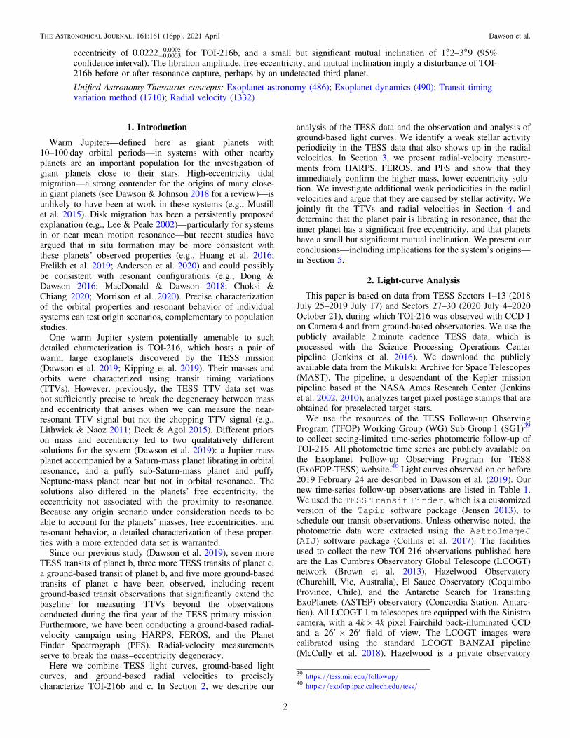
eccentricity of -+0.0222 0.0003

0.0005 for TOI-216b, and a small but significant mutual inclination of 1°.2–3°.9 (95%confidence interval). The libration amplitude, free eccentricity, and mutual inclination imply a disturbance of TOI-216b before or after resonance capture, perhaps by an undetected third planet.

Unified Astronomy Thesaurus concepts: Exoplanet astronomy (486); Exoplanet dynamics (490); Transit timingvariation method (1710); Radial velocity (1332)

1. Introduction

Warm Jupiters—defined here as giant planets with10–100 day orbital periods—in systems with other nearbyplanets are an important population for the investigation ofgiant planets close to their stars. High-eccentricity tidalmigration—a strong contender for the origins of many close-in giant planets (see Dawson & Johnson 2018 for a review)—isunlikely to have been at work in these systems (e.g., Mustillet al. 2015). Disk migration has been a persistently proposedexplanation (e.g., Lee & Peale 2002)—particularly for systemsin or near mean motion resonance—but recent studies haveargued that in situ formation may be more consistent withthese planets’ observed properties (e.g., Huang et al. 2016;Frelikh et al. 2019; Anderson et al. 2020) and could possiblybe consistent with resonant configurations (e.g., Dong &Dawson 2016; MacDonald & Dawson 2018; Choksi &Chiang 2020; Morrison et al. 2020). Precise characterizationof the orbital properties and resonant behavior of individualsystems can test origin scenarios, complementary to populationstudies.

One warm Jupiter system potentially amenable to suchdetailed characterization is TOI-216, which hosts a pair ofwarm, large exoplanets discovered by the TESS mission(Dawson et al. 2019; Kipping et al. 2019). Their masses andorbits were characterized using transit timing variations(TTVs). However, previously, the TESS TTV data set wasnot sufficiently precise to break the degeneracy between massand eccentricity that arises when we can measure the near-resonant TTV signal but not the chopping TTV signal (e.g.,Lithwick & Naoz 2011; Deck & Agol 2015). Different priorson mass and eccentricity led to two qualitatively differentsolutions for the system (Dawson et al. 2019): a Jupiter-massplanet accompanied by a Saturn-mass planet librating in orbitalresonance, and a puffy sub-Saturn-mass planet and puffyNeptune-mass planet near but not in orbital resonance. Thesolutions also differed in the planets’ free eccentricity, theeccentricity not associated with the proximity to resonance.Because any origin scenario under consideration needs to beable to account for the planets’ masses, free eccentricities, andresonant behavior, a detailed characterization of these proper-ties with a more extended data set is warranted.

Since our previous study (Dawson et al. 2019), seven moreTESS transits of planet b, three more TESS transits of planet c,a ground-based transit of planet b, and five more ground-basedtransits of planet c have been observed, including recentground-based transit observations that significantly extend thebaseline for measuring TTVs beyond the observationsconducted during the first year of the TESS primary mission.Furthermore, we have been conducting a ground-based radial-velocity campaign using HARPS, FEROS, and the PlanetFinder Spectrograph (PFS). Radial-velocity measurementsserve to break the mass–eccentricity degeneracy.

Here we combine TESS light curves, ground-based lightcurves, and ground-based radial velocities to preciselycharacterize TOI-216b and c. In Section 2, we describe our

analysis of the TESS data and the observation and analysis ofground-based light curves. We identify a weak stellar activityperiodicity in the TESS data that also shows up in the radialvelocities. In Section 3, we present radial-velocity measure-ments from HARPS, FEROS, and PFS and show that theyimmediately confirm the higher-mass, lower-eccentricity solu-tion. We investigate additional weak periodicities in the radialvelocities and argue that they are caused by stellar activity. Wejointly fit the TTVs and radial velocities in Section 4 anddetermine that the planet pair is librating in resonance, that theinner planet has a significant free eccentricity, and that planetshave a small but significant mutual inclination. We present ourconclusions—including implications for the system’s origins—in Section 5.

2. Light-curve Analysis

This paper is based on data from TESS Sectors 1–13 (2018July 25–2019 July 17) and Sectors 27–30 (2020 July 4–2020October 21), during which TOI-216 was observed with CCD 1on Camera 4 and from ground-based observatories. We use thepublicly available 2 minute cadence TESS data, which isprocessed with the Science Processing Operations Centerpipeline (Jenkins et al. 2016). We download the publiclyavailable data from the Mikulski Archive for Space Telescopes(MAST). The pipeline, a descendant of the Kepler missionpipeline based at the NASA Ames Research Center (Jenkinset al. 2002, 2010), analyzes target pixel postage stamps that areobtained for preselected target stars.We use the resources of the TESS Follow-up Observing

Program (TFOP) Working Group (WG) Sub Group 1 (SG1)39

to collect seeing-limited time-series photometric follow-up ofTOI-216. All photometric time series are publicly available onthe Exoplanet Follow-up Observing Program for TESS(ExoFOP-TESS) website.40 Light curves observed on or before2019 February 24 are described in Dawson et al. (2019). Ournew time-series follow-up observations are listed in Table 1.We used the TESS Transit Finder, which is a customizedversion of the Tapir software package (Jensen 2013), toschedule our transit observations. Unless otherwise noted, thephotometric data were extracted using the AstroImageJ(AIJ) software package (Collins et al. 2017). The facilitiesused to collect the new TOI-216 observations published hereare the Las Cumbres Observatory Global Telescope (LCOGT)network (Brown et al. 2013), Hazelwood Observatory(Churchill, Vic, Australia), El Sauce Observatory (CoquimboProvince, Chile), and the Antarctic Search for TransitingExoPlanets (ASTEP) observatory (Concordia Station, Antarc-tica). All LCOGT 1m telescopes are equipped with the Sinistrocamera, with a 4k× 4k pixel Fairchild back-illuminated CCDand a ¢ ´ ¢26 26 field of view. The LCOGT images werecalibrated using the standard LCOGT BANZAI pipeline(McCully et al. 2018). Hazelwood is a private observatory

39 https://tess.mit.edu/followup/40 https://exofop.ipac.caltech.edu/tess/

2

The Astronomical Journal, 161:161 (16pp), 2021 April Dawson et al.

with an f/8 Planewave Instruments CDK12 0.32 m telescopeand an SBIG STT3200 2.2k× 1.5k CCD, giving a ¢ ´ ¢20 13field of view. El Sauce is a private observatory that hosts anumber of telescopes; the observations reported here werecarried out with a Planewave Instruments CDK14 0.36 mtelescope and an SBIG STT-1603-3 1536k× 1024k CCD,giving a ¢ ´ ¢19 13 field of view. ASTEP is a 0.4 m telescopewith an FLI Proline 16801E 4k× 4k CCD, giving a ¢ ´ ¢63 63field of view. The ASTEP photometric data were extractedusing a custom IDL-based pipeline.

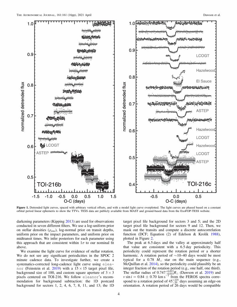
We fit the transit light curves (Figure 1) using the TAPsoftware package (Gazak et al. 2012), which implementsMarkov Chain Monte Carlo (MCMC) using the Mandel &Agol (2002) transit model and the Carter & Winn (2009)wavelet likelihood function, with the modifications describedin Dawson et al. (2014). The results are summarized in Table 2and Table 3. For TESS light curves, we use the presearch data-conditioned flux, which is corrected for systematic (e.g.,instrumental) trends using cotrending basis vectors (Smith et al.2012; Stumpe et al. 2014). For all light curves, we use theCarter & Winn (2009) wavelet likelihood function (which, forthe red noise component, assumes noise with an amplitude thatscales as frequency−1) with free parameters for the amplitudeof the red σr and white noise σr and a linear trend fitsimultaneously to each transit light-curve segment with othertransit parameters. For the ground-based observations, we fit alinear trend to airmass instead of time. We assign eachinstrument and filter (TESS, Hazelwood g′ and Rc, LCOGT i′and I, El Sauce Rc, and ASTEP Rc) its own set of limb-darkening parameters because of the different wave bands. Weuse one set of noise parameters for all the TESS light curvesand an additional set for each ground-based light curve. Weadopt uniform priors on the planet-to-star radius ratio (Rp/Rå),the impact parameter b (which can be either negative orpositive; we report |b|), the midtransit time, the limb-darkeningcoefficients q1 and q2 (Kipping 2013), and the slope andintercept of each transit segment’s linear trend. For the grazingtransits of the inner planet, we impose a uniform prior on Rp/Rå

from 0 to 0.17, with the upper limit corresponding to a planetradius of 0.13 solar radii (see Dawson et al. 2019 for detailsand justification). Despite a well-constrained transit depth

(Table 2), the inner planet’s radius ratio is highly uncertain dueto degeneracy between the radius ratio and impact parameter(see Figure 3 of Dawson et al. 2019). We also impose auniform prior on the log of the light-curve stellar density ρcirc.We use ρcirc, the stellar density derived from the light curveassuming a circular orbit, to compute the Mandel & Agol(2002) model normalized separation of centers z= d/Rå,assuming Mp=Må and a circular orbit:

r r= Å Åz P P a R 1circ1 3 2 3( ) ( ) ( ) ( )

where P is the orbital period, the subscript ⊕ denotes Earth,and the subscript e denotes the Sun. We will later combine theposteriors ρcirc from the light curve and ρå (from Dawson et al.’s2019 isochrone fit) to constrain the orbital eccentricity(Section 4.2). We perform an additional set of fits where weallow for a dilution factor for the TESS light curves and find theresults to be indistinguishable. We measure a dilution factorof -

+1.000 0.0110.012.

We also perform two additional fits to look for transitduration variations, following Dawson (2020). In the first fit,we allow the impact parameter to vary with the priorrecommended by Dawson (2020). We find tentative evidencefor the variation in the transit impact parameter for the innerplanet, with an impact parameter change scale of -

+0.007 0.0030.004. In

the second fit, we allow ρcirc (Equation (1)) and b to vary foreach transit with a prior that corresponds to a uniform prior intransit duration (Dawson 2020). Again, the inner planetexhibits tentative evidence for variation in its transit durations.We fit a line to the transit durations as a function of midtransittime and determine a 3σ confidence interval on the slope of−0.4 to 4 s day−1 for the inner planet and −1 to 0.4 s day−1 forthe outer planet.For comparison and to ensure that the results are not

sensitive to the correlated noise treatment, we also fit the lightcurves using the exoplanet package (Foreman-Mackeyet al. 2019), which uses Gaussian process regression. Each setof TESS light curves along with eight ground-based lightcurves is modeled with a light-curve transit model built fromstarry (Luger et al. 2019) plus a Matern-3/2 Gaussianprocess kernel with a white noise term. Seven sets of limb-

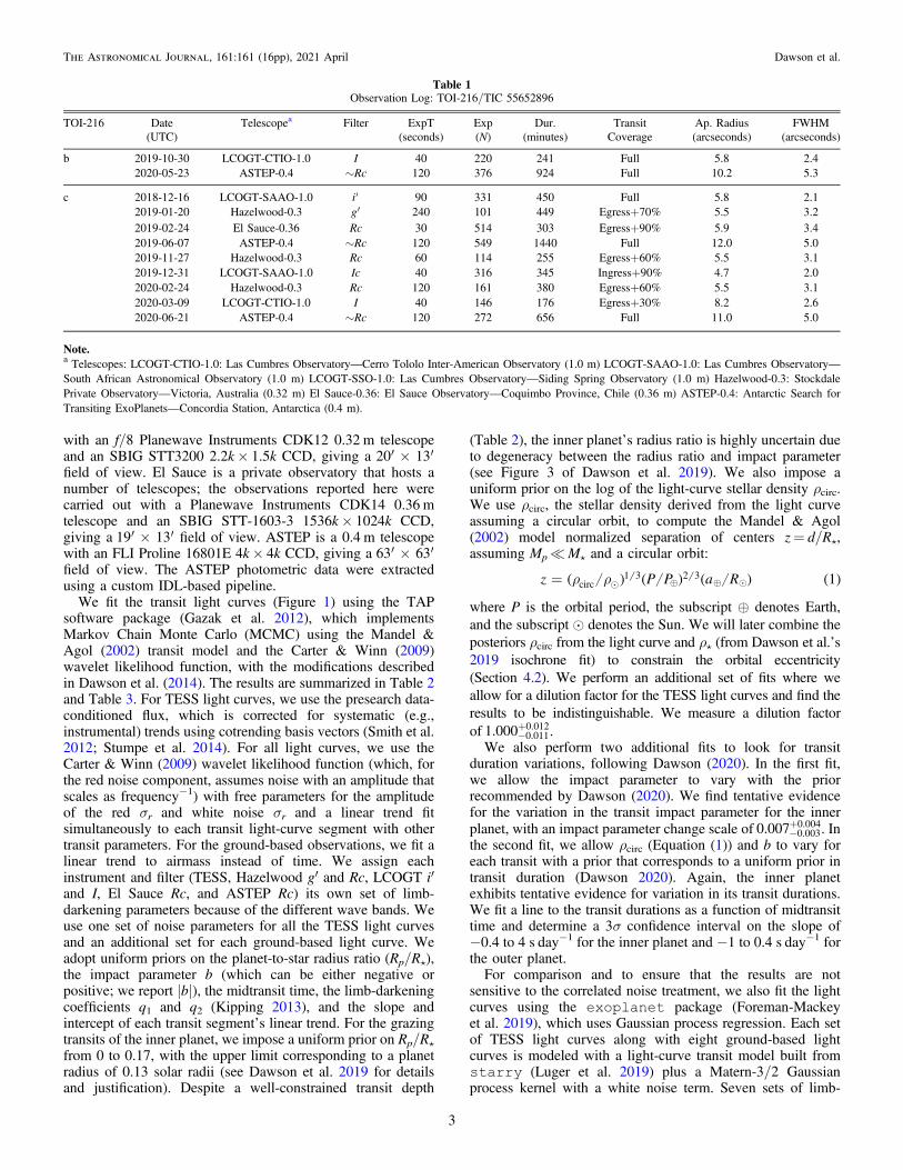
Table 1Observation Log: TOI-216/TIC 55652896

TOI-216 Date Telescopea Filter ExpT Exp Dur. Transit Ap. Radius FWHM(UTC) (seconds) (N) (minutes) Coverage (arcseconds) (arcseconds)

b 2019-10-30 LCOGT-CTIO-1.0 I 40 220 241 Full 5.8 2.42020-05-23 ASTEP-0.4 ∼Rc 120 376 924 Full 10.2 5.3

c 2018-12-16 LCOGT-SAAO-1.0 ¢i 90 331 450 Full 5.8 2.12019-01-20 Hazelwood-0.3 ¢g 240 101 449 Egress+70% 5.5 3.22019-02-24 El Sauce-0.36 Rc 30 514 303 Egress+90% 5.9 3.42019-06-07 ASTEP-0.4 ∼Rc 120 549 1440 Full 12.0 5.02019-11-27 Hazelwood-0.3 Rc 60 114 255 Egress+60% 5.5 3.12019-12-31 LCOGT-SAAO-1.0 Ic 40 316 345 Ingress+90% 4.7 2.02020-02-24 Hazelwood-0.3 Rc 120 161 380 Egress+60% 5.5 3.12020-03-09 LCOGT-CTIO-1.0 I 40 146 176 Egress+30% 8.2 2.62020-06-21 ASTEP-0.4 ∼Rc 120 272 656 Full 11.0 5.0

Note.a Telescopes: LCOGT-CTIO-1.0: Las Cumbres Observatory—Cerro Tololo Inter-American Observatory (1.0 m) LCOGT-SAAO-1.0: Las Cumbres Observatory—South African Astronomical Observatory (1.0 m) LCOGT-SSO-1.0: Las Cumbres Observatory—Siding Spring Observatory (1.0 m) Hazelwood-0.3: StockdalePrivate Observatory—Victoria, Australia (0.32 m) El Sauce-0.36: El Sauce Observatory—Coquimbo Province, Chile (0.36 m) ASTEP-0.4: Antarctic Search forTransiting ExoPlanets—Concordia Station, Antarctica (0.4 m).

3

The Astronomical Journal, 161:161 (16pp), 2021 April Dawson et al.

darkening parameters (Kipping 2013) are used for observationsconducted in seven different filters. We use a log-uniform prioron stellar densities (ρcirc), log-normal prior on transit depths,uniform prior on the impact parameters, and uniform prior onmidtransit times. We infer posteriors for each parameter usingthis approach that are consistent within 1σ to our nominal fitabove.

We examine the light curve for evidence of stellar rotation.We do not see any significant periodicities in the SPOC 2minute cadence data. To investigate further, we create asystematics-corrected long-cadence light curve using elea-nor (Feinstein et al. 2019) with a 15× 15 target pixel file,background size of 100, and custom square aperture of 3× 3pixels centered on TOI-216. We follow eleanorʼs recom-mendation for background subtraction: the 1D postcardbackground for sectors 1, 2, 4, 6, 7, 8, 11, and 13; the 1D

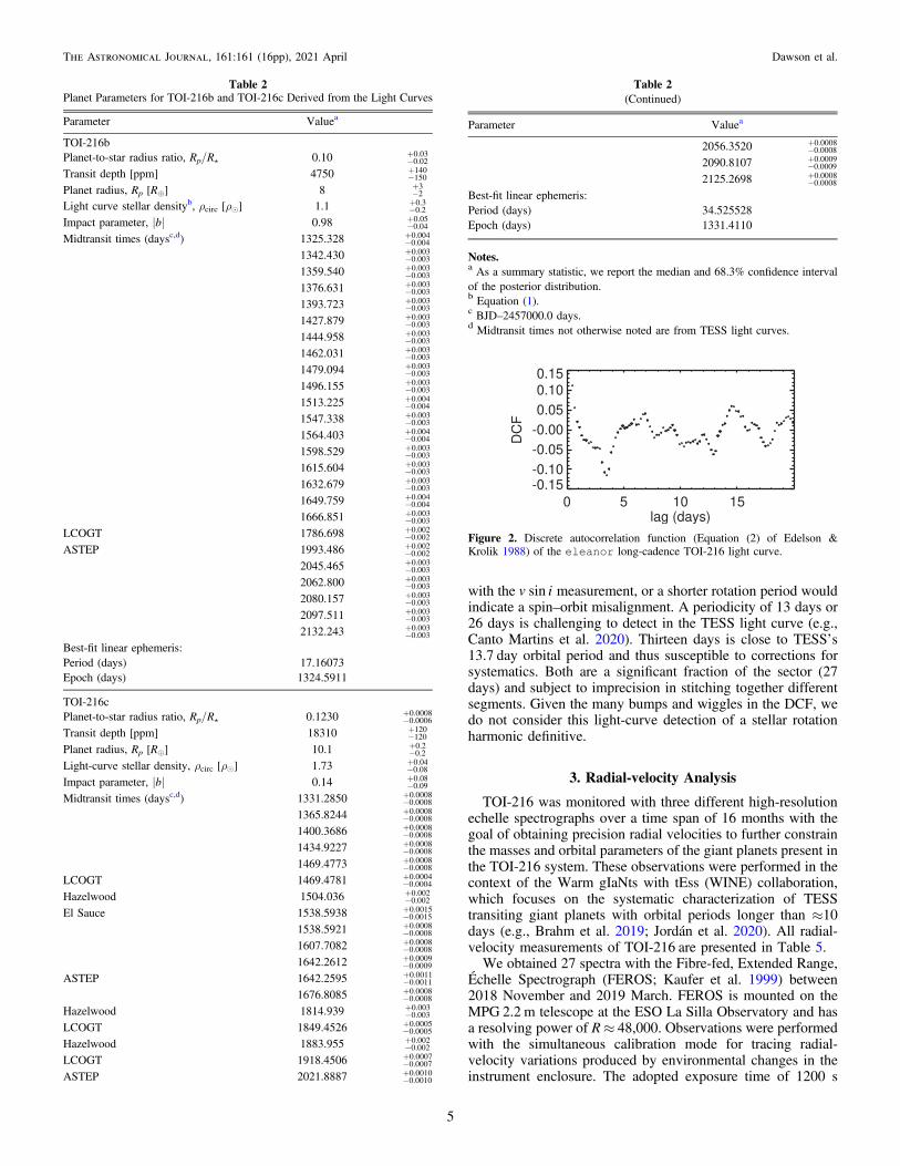
target pixel file background for sectors 3 and 5; and the 2Dtarget pixel file background for sectors 9 and 12. Then, wemask out the transits and compute a discrete autocorrelationfunction (DCF; Equation (2) of Edelson & Krolik 1988),plotted in Figure 2.The peak at 6.5 days and the valley at approximately half

that value are consistent with a 6.5 day periodicity. Thisperiodicity could represent the rotation period or a shorterharmonic. A rotation period of ∼10–40 days would be mosttypical for a 0.78 Me star on the main sequence (e.g.,McQuillan et al. 2014), so the periodicity could plausibly be aninteger fraction of the rotation period (e.g., one half, one third).The stellar radius of -

+ R0.747 0.0140.015

(Dawson et al. 2019) and= v isin 0.84 0.70 km s−1 from the FEROS spectra corre-

spond to a rotation period of -+45 20

225 days assuming an edge-onorientation. A rotation period of 26 days would be compatible

Figure 1. Detrended light curves, spaced with arbitrary vertical offsets, and with a model light curve overplotted. The light curves are phased based on a constantorbital period linear ephemeris to show the TTVs. TESS data are publicly available from MAST and ground-based data from the ExoFOP-TESS website.

4

The Astronomical Journal, 161:161 (16pp), 2021 April Dawson et al.

with the v isin measurement, or a shorter rotation period wouldindicate a spin–orbit misalignment. A periodicity of 13 days or26 days is challenging to detect in the TESS light curve (e.g.,Canto Martins et al. 2020). Thirteen days is close to TESS’s13.7 day orbital period and thus susceptible to corrections forsystematics. Both are a significant fraction of the sector (27days) and subject to imprecision in stitching together differentsegments. Given the many bumps and wiggles in the DCF, wedo not consider this light-curve detection of a stellar rotationharmonic definitive.

3. Radial-velocity Analysis

TOI-216 was monitored with three different high-resolutionechelle spectrographs over a time span of 16 months with thegoal of obtaining precision radial velocities to further constrainthe masses and orbital parameters of the giant planets present inthe TOI-216 system. These observations were performed in thecontext of the Warm gIaNts with tEss (WINE) collaboration,which focuses on the systematic characterization of TESStransiting giant planets with orbital periods longer than ≈10days (e.g., Brahm et al. 2019; Jordán et al. 2020). All radial-velocity measurements of TOI-216 are presented in Table 5.We obtained 27 spectra with the Fibre-fed, Extended Range,

Échelle Spectrograph (FEROS; Kaufer et al. 1999) between2018 November and 2019 March. FEROS is mounted on theMPG 2.2 m telescope at the ESO La Silla Observatory and hasa resolving power of R≈ 48,000. Observations were performedwith the simultaneous calibration mode for tracing radial-velocity variations produced by environmental changes in theinstrument enclosure. The adopted exposure time of 1200 s

Table 2Planet Parameters for TOI-216b and TOI-216c Derived from the Light Curves

Parameter Valuea

TOI-216bPlanet-to-star radius ratio, Rp/Rå 0.10 -

+0.020.03

Transit depth [ppm] 4750 -+

150140

Planet radius, Rp [R⊕] 8 -+

23

Light curve stellar densityb, ρcirc [ρe] 1.1 -+

0.20.3

Impact parameter, |b| 0.98 -+

0.040.05

Midtransit times (daysc,d) 1325.328 -+

0.0040.004

1342.430 -+

0.0030.003

1359.540 -+

0.0030.003

1376.631 -+

0.0030.003

1393.723 -+

0.0030.003

1427.879 -+

0.0030.003

1444.958 -+

0.0030.003

1462.031 -+

0.0030.003

1479.094 -+

0.0030.003

1496.155 -+

0.0030.003

1513.225 -+

0.0040.004

1547.338 -+

0.0030.003

1564.403 -+

0.0040.004

1598.529 -+

0.0030.003

1615.604 -+

0.0030.003

1632.679 -+

0.0030.003

1649.759 -+

0.0040.004

1666.851 -+

0.0030.003

LCOGT 1786.698 -+

0.0020.002

ASTEP 1993.486 -+

0.0020.002

2045.465 -+

0.0030.003

2062.800 -+

0.0030.003

2080.157 -+

0.0030.003

2097.511 -+

0.0030.003

2132.243 -+

0.0030.003

Best-fit linear ephemeris:Period (days) 17.16073Epoch (days) 1324.5911

TOI-216cPlanet-to-star radius ratio, Rp/Rå 0.1230 -

+0.00060.0008

Transit depth [ppm] 18310 -+

120120

Planet radius, Rp [R⊕] 10.1 -+

0.20.2

Light-curve stellar density, ρcirc [ρe] 1.73 -+

0.080.04

Impact parameter, |b| 0.14 -+

0.090.08

Midtransit times (daysc,d) 1331.2850 -+

0.00080.0008

1365.8244 -+

0.00080.0008

1400.3686 -+

0.00080.0008

1434.9227 -+

0.00080.0008

1469.4773 -+

0.00080.0008

LCOGT 1469.4781 -+

0.00040.0004

Hazelwood 1504.036 -+

0.0020.002

El Sauce 1538.5938 -+

0.00150.0015

1538.5921 -+

0.00080.0008

1607.7082 -+

0.00080.0008

1642.2612 -+

0.00090.0009

ASTEP 1642.2595 -+

0.00110.0011

1676.8085 -+

0.00080.0008

Hazelwood 1814.939 -+

0.0030.003

LCOGT 1849.4526 -+

0.00050.0005

Hazelwood 1883.955 -+

0.0020.002

LCOGT 1918.4506 -+

0.00070.0007

ASTEP 2021.8887 -+

0.00100.0010

Table 2(Continued)

Parameter Valuea

2056.3520 -+

0.00080.0008

2090.8107 -+

0.00090.0009

2125.2698 -+

0.00080.0008

Best-fit linear ephemeris:Period (days) 34.525528Epoch (days) 1331.4110

Notes.a As a summary statistic, we report the median and 68.3% confidence intervalof the posterior distribution.b Equation (1).c BJD–2457000.0 days.d Midtransit times not otherwise noted are from TESS light curves.

Figure 2. Discrete autocorrelation function (Equation (2) of Edelson &Krolik 1988) of the eleanor long-cadence TOI-216 light curve.

5

The Astronomical Journal, 161:161 (16pp), 2021 April Dawson et al.

yielded spectra with signal-to-noise ratios in the range from 40to 75. FEROS spectra were processed from raw data with theceres pipeline (Brahm et al. 2017), which delivers precisionradial velocities and line bisector span measurements via cross-correlation with a binary mask resembling the spectralproperties of a G2-type star. The radial-velocity uncertaintiesfor the FEROS observations of TOI-216 range between 7 and15 m s−1. We remove two outliers from the FEROS radial-velocity time series at 1503.75 and 1521.57 days. Allsubsequent results do not include these outliers. We havechecked that no results except the inferred jitter for the FEROSdata set are sensitive to whether or not the outliers are included.

We observed TOI-216 on 15 different epochs between 2018December and 2019 October with the High Accuracy Radialvelocity Planet Searcher (HARPS; Mayor et al. 2003) mountedon the ESO 3.6 m telescope at the ESO La Silla Observatory, inChile. We adopted an exposure time of 1800 s for theseobservations using the high-radial-velocity accuracy mode(HAM; R≈ 115,000), which produced spectra with signal-to-noise ratios of ≈40 per resolution element. As in the case ofFEROS, HARPS data for TOI-216 was processed with theceres pipeline, delivering radial-velocity measurements withtypical errors of ≈5 m s−1.

TOI-216 was also monitored with the PFS (Crane et al.2006, 2008, 2010) mounted on the 6.5 m Magellan II ClayTelescope at Las Campanas Observatory (LCO), in Chile.These spectra were obtained on 18 different nights, between2018 December and 2020 March, using the 0 3× 2 5 slit,which delivers a resolving power of R= 130,000. Due to itsmoderate faintness, TOI-216 was observed with the 3× 3binning mode to minimize read-out noise, and an exposure timeof 1200 s was adopted to reach a radial-velocity precisionof≈ 2 m s−1. An iodine cell was used in these observations asa reference for the wavelength calibration. The PFS data wereprocessed with a custom IDL pipeline (Butler et al. 1996).Three consecutive 1200 s iodine-free exposures of TOI-216were obtained to construct a stellar spectral template for

disentangling the iodine spectra from the stellar one forcomputing the radial velocities.It is immediately evident that the radial velocities show good

agreement with Dawson et al.ʼs (2019) higher-mass solution,which was fit to the earlier, transit-time-only data set (Figure 3),and with the solution of Kipping et al. (2019) based on transittimes from the first six sectors. The bottom panel of Figure 3shows the radial velocities phased to the outer planet’s orbitalperiod. We compute a generalized Lomb–Scargle periodogram(Cumming et al. 1999; Zechmeister & Kürster 2009) in Figures 4and 5. The x-axis is frequency f in cycles per day. The y-axis is thesquare root of the power, where we define power as

=S - S

Ss s

s

-

Power2

, 2f

iv v

iv

i1

i f i

i

i

i

i

, ,02

2,02

2

2

( )

( )

where σi is the reported uncertainty (Table 5) and vi,0 is the

radial-velocity (Table 5) with the error weighted meansS

s

vi i i2

1

i2

for each of the three data sets (PFS, HARPS, and FEROS)subtracted. The sinusoidal function vi,f is

p p= - + - +v A f t t BA f t t Ccos 2 sin 2 , 3i f i i k, 0 0[ ( )] [ ( )] ( )

where A and B are computed following Zechmeister & Kürster(2009), k is each of the three data sets, t0 is the time of the firstobserved radial velocity, and

= -S

S

p ps

s

- + -

C . 4k

iA f t t BA f t t

i

cos 2 sin 2

1

i i

i

i

0 02

2

( )( [ ( )] [ ( )])

We see a peak in the periodogram at planet c’s orbital period(Figure 4, left panel). The noise-free planet c model (overplotted,dashed; a Keplerian signal computed using the parameters ofplanet c from Table 4 sampled at the observed times in Table 5)shows that many of the other peaks seen in the three periodograms

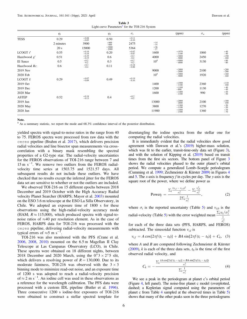
Table 3Light-curve Parametersa for the TOI-216 System

q1 q2 σr (ppm) σw (ppm)

TESS 0.29 -+

0.050.08 0.50 -

+0.100.11

2 minutes 3900 -+

600600 2475 -

+1414

20 s 15000 -+

20002000 5364 -

+2726

LCOGT i′ 0.55 -+

0.100.10 0.20 -

+0.070.07 1600 -

+11001970 1060 -

+4040

Hazelwood g′ 0.51 -+

0.150.25 0.6 -

+0.20.2 4000 -

+30003000 2450 -

+180190

El Sauce 0.5 -+

0.20.2 0.3 -

+0.20.2 104 -

+40004000 3130 -

+8080

Hazelwood Rc: 0.6 -+

0.40.3 0.11 -

+0.080.18

2019 Nov 9000 -+

20003000 2100 -

+200200

2020 Feb 104 -+

30003000 1920 -

+160160

LCOGT I: 0.29 -+

0.090.07 0.49 -

+0.100.19

2019 Oct 1400 -+

11001500 2360 -

+100110

2019 Dec 1200 -+

8001100 1130 -

+4040

2020 Mar 1600 -+

11001400 990 -

+5050

ASTEP 0.52 -+

0.130.18 0.4 -

+0.20.2

2019 Jun 13000 -+

20002000 2100 -

+100100

2020 May 3800 -+

11001300 1270 -

+5050

2020 Jun 11900 -+

15001500 1360 -

+7070

Note.a As a summary statistic, we report the mode and 68.3% confidence interval of the posterior distribution.

6

The Astronomical Journal, 161:161 (16pp), 2021 April Dawson et al.

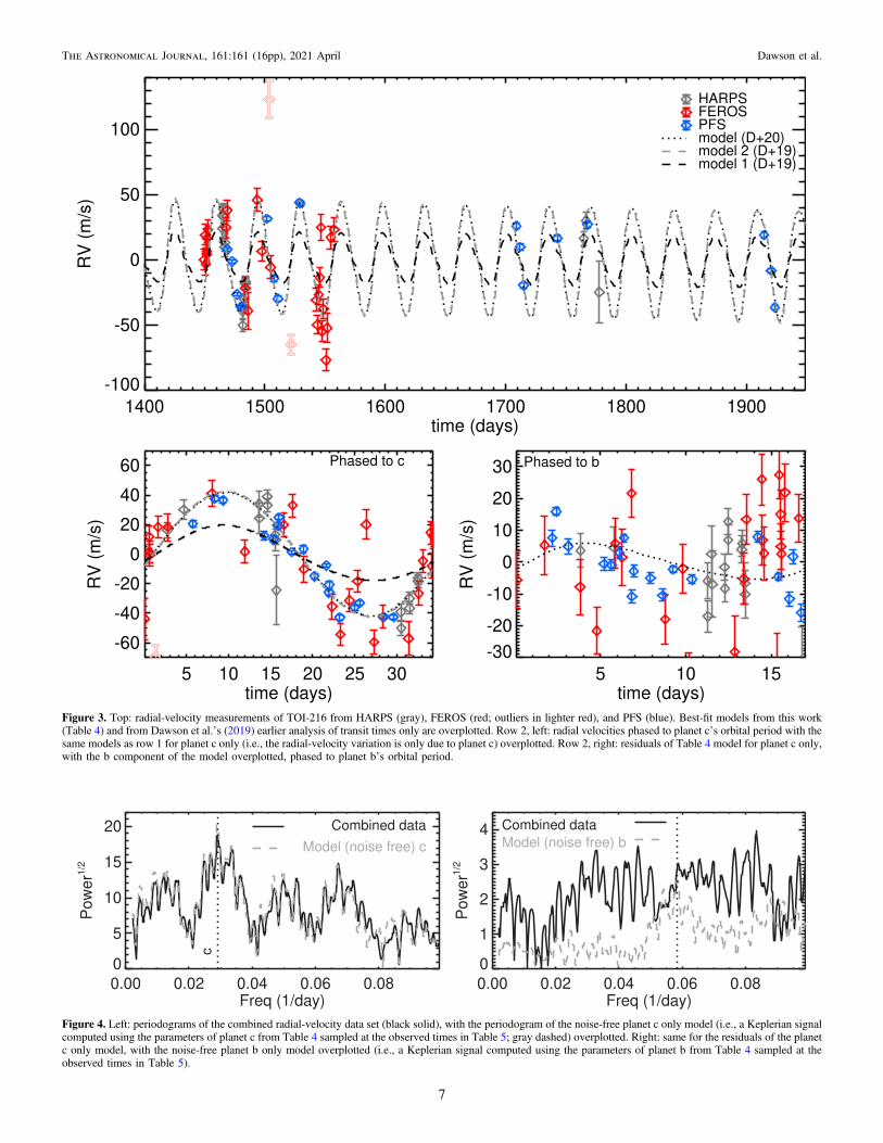
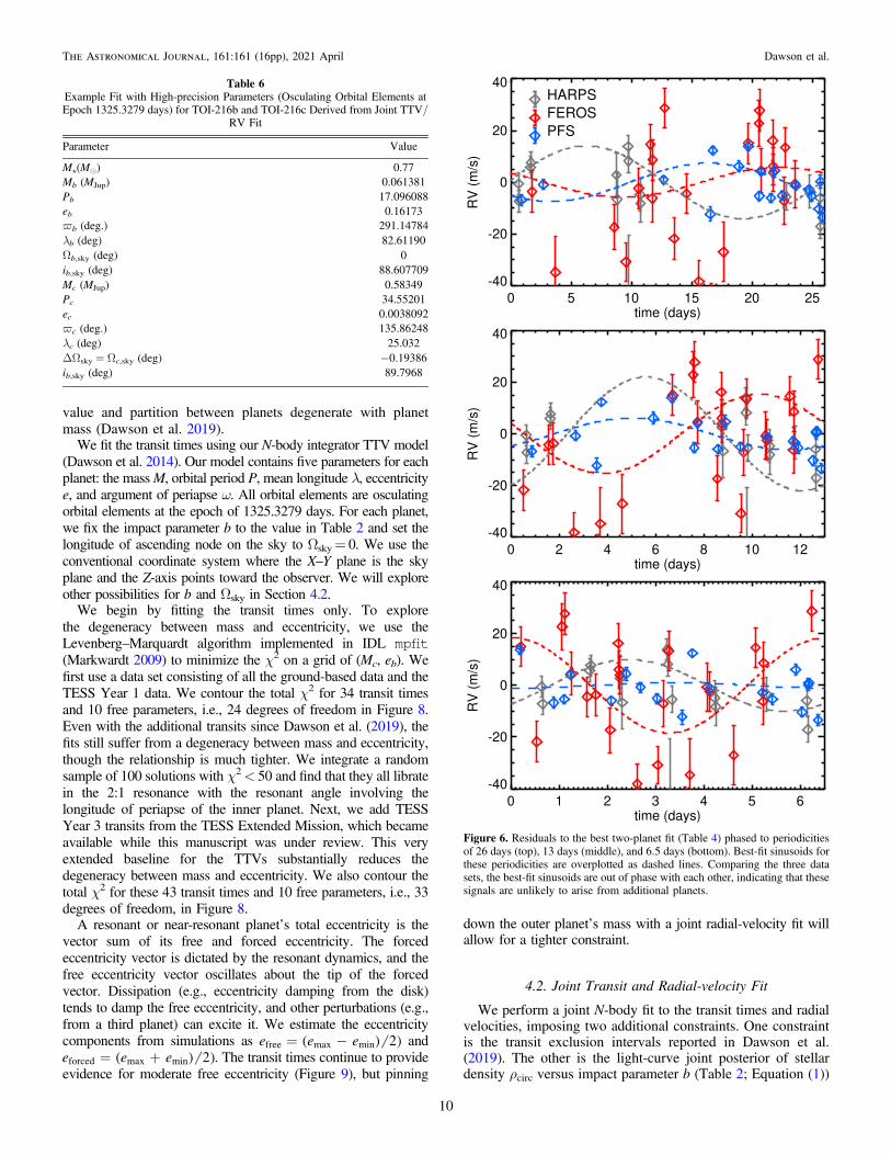
Figure 3. Top: radial-velocity measurements of TOI-216 from HARPS (gray), FEROS (red; outliers in lighter red), and PFS (blue). Best-fit models from this work(Table 4) and from Dawson et al.ʼs (2019) earlier analysis of transit times only are overplotted. Row 2, left: radial velocities phased to planet c’s orbital period with thesame models as row 1 for planet c only (i.e., the radial-velocity variation is only due to planet c) overplotted. Row 2, right: residuals of Table 4 model for planet c only,with the b component of the model overplotted, phased to planet b’s orbital period.

Figure 4. Left: periodograms of the combined radial-velocity data set (black solid), with the periodogram of the noise-free planet c only model (i.e., a Keplerian signalcomputed using the parameters of planet c from Table 4 sampled at the observed times in Table 5; gray dashed) overplotted. Right: same for the residuals of the planetc only model, with the noise-free planet b only model overplotted (i.e., a Keplerian signal computed using the parameters of planet b from Table 4 sampled at theobserved times in Table 5).

7

The Astronomical Journal, 161:161 (16pp), 2021 April Dawson et al.

are aliases of planet c’s orbital period (i.e., they are caused by theobservational time sampling of the planet’s signal). Planet b’ssignal is below the noise level (Figure 3, bottom-right panel;Figure 4, right panels). In the PFS data set, including planet bimproves the chi-squared from 403 to 328 (for 18 data points and 5additional parameters); for the HARPS and FEROS data sets, thereis no improvement in chi-squared. Given that planet b is barelydetected, we cannot rule out other planets in the system withsmaller orbital radial-velocity amplitudes.Systems containing an outer planet in or near a 2:1 mean

motion resonance with a less-massive inner planet can bemistaken for a single eccentric planet, because the first-eccentricity harmonic appears at half the planet’s orbital period(e.g., Anglada-Escudé et al. 2010; Kürster et al. 2015). In thecase of the system TOI-216, the lack of detection of TOI-216bis not due to this phenomenon because the solution we subtractoff for planet c has near-zero eccentricity. However, withoutprior knowledge that the system contains a resonant pair, if weonly had the radial-velocity data sets and the data sets were lessnoisy (or had more data points), we might be sensitive to planetb’s signal but mistakenly interpret it as planet c’s eccentricity.The residuals of the two-planet fit (and one-planet fit) show

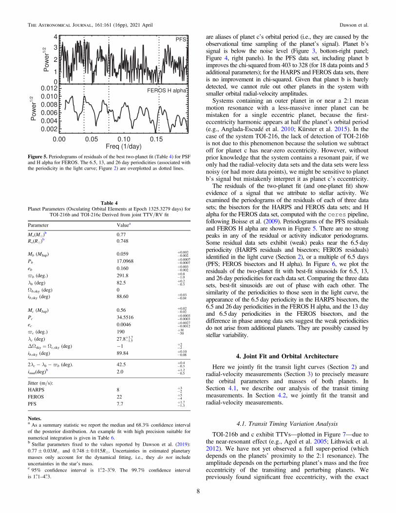
evidence of a signal that we attribute to stellar activity. Weexamined the periodograms of the residuals of each of three datasets; the bisectors for the HARPS and FEROS data sets; and Halpha for the FEROS data set, computed with the ceres pipeline,following Boisse et al. (2009). Periodograms of the PFS residualsand FEROS H alpha are shown in Figure 5. There are no strongpeaks in any of the residual or activity indicator periodograms.Some residual data sets exhibit (weak) peaks near the 6.5 dayperiodicity (HARPS residuals and bisectors; FEROS residuals)identified in the light curve (Section 2), or a multiple of 6.5 days(PFS; FEROS bisectors and H alpha). In Figure 6, we plot theresiduals of the two-planet fit with best-fit sinusoids for 6.5, 13,and 26 day periodicities for each data set. Comparing the three datasets, best-fit sinusoids are out of phase with each other. Thesimilarity of the periodicities to those seen in the light curve, theappearance of the 6.5 day periodicity in the HARPS bisectors, the6.5 and 26 day periodicities in the FEROS H alpha, and the 13 dayand 6.5 day periodicities in the FEROS bisectors, and thedifference in phase among data sets suggest the weak periodicitiesdo not arise from additional planets. They are possibly caused bystellar variability.

4. Joint Fit and Orbital Architecture

Here we jointly fit the transit light curves (Section 2) andradial-velocity measurements (Section 3) to precisely measurethe orbital parameters and masses of both planets. InSection 4.1, we describe our analysis of the transit timingmeasurements. In Section 4.2, we jointly fit the transit andradial-velocity measurements.

4.1. Transit Timing Variation Analysis

TOI-216b and c exhibit TTVs—plotted in Figure 7—due tothe near-resonant effect (e.g., Agol et al. 2005; Lithwick et al.2012). We have not yet observed a full super-period (whichdepends on the planets’ proximity to the 2:1 resonance). Theamplitude depends on the perturbing planet’s mass and the freeeccentricity of the transiting and perturbing planets. Wepreviously found significant free eccentricity, with the exact

Figure 5. Periodograms of residuals of the best two-planet fit (Table 4) for PSFand H alpha for FEROS. The 6.5, 13, and 26 day periodicities (associated withthe periodicity in the light curve; Figure 2) are overplotted as dotted lines.

Table 4Planet Parameters (Osculating Orbital Elements at Epoch 1325.3279 days) for

TOI-216b and TOI-216c Derived from joint TTV/RV fit

Parameter Valuea

Må(Me)b 0.77

Rå(Re)b 0.748

Mb (MJup) 0.059 -+

0.0020.002

Pb 17.0968 -+

0.00070.0007

eb 0.160 -+

0.0020.003

ϖb (deg.) 291.8 -+

1.00.8

λb (deg) 82.5 -+

0.30.2

Ωb,sky (deg) 0ib,sky (deg) 88.60 -

+0.040.03

Mc (MJup) 0.56 -+

0.020.02

Pc 34.5516 -+

0.00030.0003

ec 0.0046 -+

0.00120.0027

ϖc (deg.) 190 -+

5030

λc (deg) -+27.8 1.5

1.7

ΔΩsky = Ωc,sky (deg) −1 -+

22

ib,sky (deg) 89.84 -+

0.080.10

2λc − λb − ϖb (deg). 42.5 -+

0.30.4

imut(deg)b 2.0 -

+0.51.2

Jitter (m/s):HARPS 8 -

+23

FEROS 22 -+

45

PFS 7.7 -+

1.31.7

Notes.a As a summary statistic we report the median and 68.3% confidence intervalof the posterior distribution. An example fit with high precision suitable fornumerical integration is given in Table 6.b Stellar parameters fixed to the values reported by Dawson et al. (2019):0.77 ± 0.03Me and 0.748 ± 0.015Re. Uncertainties in estimated planetarymasses only account for the dynamical fitting, i.e., they do not includeuncertainties in the starʼs mass.c 95% confidence interval is 1°. 2–3°. 9. The 99.7% confidence intervalis 1°. 1–4°. 3.

8

The Astronomical Journal, 161:161 (16pp), 2021 April Dawson et al.

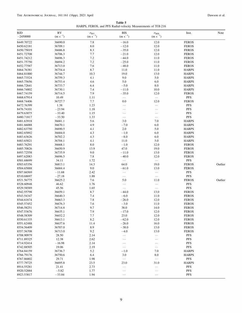
Table 5HARPS, FEROS, and PFS Radial-velocity Measurements of TOI-216

BJD RV σRV BIS σBIS Inst. Note−2450000 (m s−1) (m s−1) (m s−1) (m s−1)

8449.70722 36690.0 7.8 −16.0 12.0 FEROS8450.62181 36709.1 8.0 −12.0 12.0 FEROS8450.75019 36686.8 8.3 −35.0 12.0 FEROS8451.72708 36706.3 7.7 −21.0 12.0 FEROS8451.74212 36696.3 7.2 −44.0 11.0 FEROS8451.75750 36694.2 7.2 −25.0 11.0 FEROS8452.77587 36713.0 7.6 −48.0 11.0 FEROS8464.76381 36754.4 8.7 11.0 11.0 HARPS8464.81000 36744.7 10.3 19.0 13.0 HARPS8465.73524 36759.3 4.1 9.0 5.0 HARPS8465.75656 36753.4 4.6 5.0 6.0 HARPS8466.72641 36733.7 6.4 −5.0 8.0 HARPS8466.74802 36730.1 7.4 −11.0 10.0 HARPS8467.74159 36714.5 7.9 −35.0 12.0 FEROS8468.67914 10.49 1.11 L L PFS8468.74406 36727.7 7.7 0.0 12.0 FEROS8472.76399 1.38 1.23 L L PFS8476.74101 −23.94 1.18 L L PFS8479.63075 −33.40 1.15 L L PFS8480.71817 −33.50 1.33 L L PFS8481.63918 36681.1 5.6 3.0 7.0 HARPS8481.66088 36670.1 4.9 −7.0 6.0 HARPS8482.63750 36690.5 4.1 2.0 5.0 HARPS8482.65892 36684.0 4.3 −1.0 6.0 HARPS8483.63626 36702.2 4.3 −8.0 6.0 HARPS8483.65821 36704.1 4.1 11.0 5.0 HARPS8483.76291 36668.1 8.0 −1.0 12.0 FEROS8485.70826 36650.9 13.9 47.0 19.0 FEROS8493.72558 36735.9 9.0 −11.0 13.0 FEROS8497.62083 36696.5 7.8 −40.0 12.0 FEROS8501.68699 34.11 1.72 L L PFS8503.65356 36813.1 14.3 64.0 19.0 FEROS Outlier8504.65888 36684.4 9.0 −61.0 13.0 FEROS8507.66569 −11.68 2.42 L L PFS8510.68697 −27.18 1.88 L L PFS8521.56775 36625.2 7.6 5.0 11.0 FEROS Outlier8528.60948 46.62 1.76 L L PFS8529.58589 45.56 1.65 L L PFS8542.55798 36659.1 8.7 −44.0 13.0 FEROS8543.54347 36640.3 7.4 −6.0 11.0 FEROS8544.61674 36663.3 7.8 −26.0 12.0 FEROS8545.57452 36676.3 7.6 −3.0 11.0 FEROS8546.58251 36714.8 9.7 38.0 14.0 FEROS8547.53676 36635.1 7.9 −17.0 12.0 FEROS8548.58309 36652.2 7.7 23.0 12.0 FEROS8550.61335 36613.1 8.2 −62.0 12.0 FEROS8551.62488 36637.6 11.4 −26.0 16.0 FEROS8554.56409 36707.0 8.9 −38.0 13.0 FEROS8557.56708 36713.0 9.2 −4.0 13.0 FEROS8708.90979 28.50 2.14 L L PFS8711.89325 12.38 2.62 L L PFS8714.92414 −16.98 2.14 L L PFS8742.88505 19.06 2.19 L L PFS8764.84159 36736.7 5.2 −1.0 7.0 HARPS8766.79176 36750.6 6.4 3.0 8.0 HARPS8767.86802 29.71 1.98 L L PFS8777.79725 36695.8 23.5 23.0 31.0 HARPS8914.55281 21.41 2.73 L L PFS8920.52884 −5.82 1.77 L L PFS8923.53817 −33.84 1.94 L L PFS

9

The Astronomical Journal, 161:161 (16pp), 2021 April Dawson et al.

value and partition between planets degenerate with planetmass (Dawson et al. 2019).

We fit the transit times using our N-body integrator TTV model(Dawson et al. 2014). Our model contains five parameters for eachplanet: the massM, orbital period P, mean longitude λ, eccentricitye, and argument of periapse ω. All orbital elements are osculatingorbital elements at the epoch of 1325.3279 days. For each planet,we fix the impact parameter b to the value in Table 2 and set thelongitude of ascending node on the sky to Ωsky= 0. We use theconventional coordinate system where the X–Y plane is the skyplane and the Z-axis points toward the observer. We will exploreother possibilities for b and Ωsky in Section 4.2.

We begin by fitting the transit times only. To explorethe degeneracy between mass and eccentricity, we use theLevenberg–Marquardt algorithm implemented in IDL mpfit(Markwardt 2009) to minimize the χ2 on a grid of (Mc, eb). Wefirst use a data set consisting of all the ground-based data and theTESS Year 1 data. We contour the total χ2 for 34 transit timesand 10 free parameters, i.e., 24 degrees of freedom in Figure 8.Even with the additional transits since Dawson et al. (2019), thefits still suffer from a degeneracy between mass and eccentricity,though the relationship is much tighter. We integrate a randomsample of 100 solutions with χ2< 50 and find that they all libratein the 2:1 resonance with the resonant angle involving thelongitude of periapse of the inner planet. Next, we add TESSYear 3 transits from the TESS Extended Mission, which becameavailable while this manuscript was under review. This veryextended baseline for the TTVs substantially reduces thedegeneracy between mass and eccentricity. We also contour thetotal χ2 for these 43 transit times and 10 free parameters, i.e., 33degrees of freedom, in Figure 8.

A resonant or near-resonant planet’s total eccentricity is thevector sum of its free and forced eccentricity. The forcedeccentricity vector is dictated by the resonant dynamics, and thefree eccentricity vector oscillates about the tip of the forcedvector. Dissipation (e.g., eccentricity damping from the disk)tends to damp the free eccentricity, and other perturbations (e.g.,from a third planet) can excite it. We estimate the eccentricitycomponents from simulations as = -e e e 2free max min( ) ) and

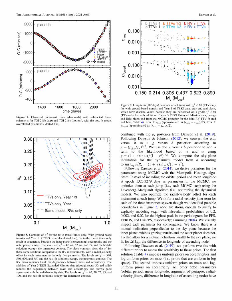
= +e e e 2forced max min( ) ). The transit times continue to provideevidence for moderate free eccentricity (Figure 9), but pinning

down the outer planet’s mass with a joint radial-velocity fit willallow for a tighter constraint.

4.2. Joint Transit and Radial-velocity Fit

We perform a joint N-body fit to the transit times and radialvelocities, imposing two additional constraints. One constraintis the transit exclusion intervals reported in Dawson et al.(2019). The other is the light-curve joint posterior of stellardensity ρcirc versus impact parameter b (Table 2; Equation (1))

Figure 6. Residuals to the best two-planet fit (Table 4) phased to periodicitiesof 26 days (top), 13 days (middle), and 6.5 days (bottom). Best-fit sinusoids forthese periodicities are overplotted as dashed lines. Comparing the three datasets, the best-fit sinusoids are out of phase with each other, indicating that thesesignals are unlikely to arise from additional planets.

Table 6Example Fit with High-precision Parameters (Osculating Orbital Elements atEpoch 1325.3279 days) for TOI-216b and TOI-216c Derived from Joint TTV/

RV Fit

Parameter Value

Må(Me) 0.77Mb (MJup) 0.061381Pb 17.096088eb 0.16173ϖb (deg.) 291.14784λb (deg) 82.61190Ωb,sky (deg) 0ib,sky (deg) 88.607709Mc (MJup) 0.58349Pc 34.55201ec 0.0038092ϖc (deg.) 135.86248λc (deg) 25.032ΔΩsky = Ωc,sky (deg) −0.19386ib,sky (deg) 89.7968

10

The Astronomical Journal, 161:161 (16pp), 2021 April Dawson et al.

combined with the ρå posterior from Dawson et al. (2019).Following Dawson & Johnson (2012), we convert the ρcircversus b to a g versus b posterior according to

r r= g circ1 3( ) . We use the g versus b posterior to add a

term to the likelihood based on e and ω usingw= + -g e e1 sin 1 2 1 2( ) ( ) . We compute the sky-plane

inclination for the dynamical model from b accordingto w= + -i a R e esin 1 sin 1sky

2( ) ( ).Following Dawson et al. (2014), we derive posteriors for the

parameters using MCMC with the Metropolis–Hastings algo-rithm. Instead of including the orbital period and mean longitudeat epoch 1325.3279 days as parameters in the MCMC, weoptimize them at each jump (i.e., each MCMC step) using theLevenberg–Marquardt algorithm (i.e., optimizing the dynamicalmodel). We also optimize the radial-velocity offset for eachinstrument at each jump. We fit for a radial-velocity jitter term foreach of the three instruments; even though we identified possibleperiodicities in Figure 5, none are strong enough to justify toexplicitly modeling (e.g., with false-alarm probabilities of 0.2,0.002, and 0.02 for the highest peak in the periodogram for PFS,FEROS, and HARPS, respectively; Cumming 2004). We visuallyinspect each parameter for convergence. We know there is amutual inclination perpendicular to the sky plane because theinner planet exhibits grazing transits and the outer planet does not.To also allow for a mutual inclination parallel to the sky plane, wefit for ΔΩsky, the difference in longitude of ascending node.Following Dawson et al. (2019), we perform two fits with

different priors to assess the sensitivity to these priors. The firstsolution (Table 4) imposes uniform priors on eccentricities andlog-uniform priors on mass (i.e., priors that are uniform in logspace). The second imposes uniform priors on mass and log-uniform priors on eccentricity. All other fitted parameters(orbital period, mean longitude, argument of periapse, radial-velocity jitters, difference in longitude of ascending node) have

Figure 7. Observed midtransit times (diamonds) with subtracted linearephemeris for TOI-216b (top) and TOI-216c (bottom), with the best-fit modeloverplotted (diamonds, dotted line).

Figure 8. Contours of χ2 for the fit to transit times only. With ground-basedtransits and Year 1 of TESS data (blue dotted line), fits to the transit times onlyresult in degeneracy between the inner planet’s (osculating) eccentricity and theouter planet’s mass. The levels are χ2 = 42, 47, 52, 62, and 77, and the best-fitsolutions occupy the innermost contour. The black contours show the χ2 forthese same solutions compared to the RV measurements, with a radial-velocityoffset for each instrument as the only free parameter. The levels are χ2 = 540,560, 600, and 650 and the best-fit solutions occupy the innermost contour. TheRV measurements break the degeneracy between mass and eccentricity. Theaddition of Year 3 TESS Extended Mission data (through sector 30; red solid)reduces the degeneracy between mass and eccentricity and shows goodagreement with the radial-velocity data. The levels are χ2 = 65, 70, 75, 85, and100, and the best-fit solutions occupy the innermost contour.

Figure 9. Long-term (106 days) behavior of solutions with χ2 < 60 (TTV-onlyfits with ground-based transits and Year 1 of TESS data, gray and and black,which have discrete values because they are performed on a grid); χ2 < 80(TTV-only fits with addition of Year 3 TESS Extended Mission data, orangeand light blue); and from the MCMC posterior for the joint RV-TTV fit (redand blue, Table 4). Row 1: efree (approximated as -e e 2max min( ) ); Row 2:eforced (approximated as +e e 2max min( ) ).

11

The Astronomical Journal, 161:161 (16pp), 2021 April Dawson et al.

uniform priors. With the data set in Dawson et al. (2019), theresults were very sensitive to the priors; with the new data setthat includes radial velocities and an expanded TTV baseline,the results with different priors are nearly indistinguishable. Inboth cases, we impose the 3σ limits on change in transitduration derived in Section 2. We measure a small butsignificant mutual inclination of 1°.2–3°.9 (95% confidenceinterval). An example fit with high precision suitable fornumerical integration is given in Table 6.

To ensure that our results are robust and that the parameterspace has been thoroughly explored by the fitting algorithm(particularly the degeneracy between eccentricity and mass), wecarry out a fit using a different N-body code and fitting algorithm.We use the Python Tool for Transit Variations (PyTTV;Korth 2020) to fit the transit times (Table 2), radial velocities(Table 5), and the stellar parameters reported in Dawson (2020).The parameter estimation is carried out by a joint N-body fit usingRebound with the IAS15 integrator (Rein & Liu 2012; Rein &Spiegel 2015) and Reboundx (Tamayo et al. 2020), to model allof the observables without approximations. Within the simulation,carried out in barycentric coordinates, a common coordinatesystem was chosen where the x–y plane is the plane of sky. The x-axis points to the east, the y-axis points to the north, and the z-axispoints to the observer. Ω is measured from east to north, and ω ismeasured from the plane of sky. For the parameter estimation withPyTTV, the gravitational forces between the planets and theinfluence of general relativity (GR) were considered, in case theinfluence of GR is significant enough to be visible in the TTVs; forthis system, general relativistic precession does not significantlyaffect the TTVs. The parameter estimation is initialized usingRayleigh priors on eccentricities (Van Eylen et al. 2019) anduniform priors on log values for the planetary masses. Theestimation of physical quantities from the TTV signal is done intwo steps. First, the posterior mode is found using the differentialevolution algorithm implemented in PyTransit (Parviainen2015). The optimization is carried out varying the planetarymasses, orbital periods, inclinations, eccentricities and argumentsof periastron. The eccentricity and argument of periastron aremapped from sampling parameters we cos and we sin . Thelongitudes of the ascending nodes are fixed for both planets. Afterthe posterior mode is found, a sample from the posterior isobtained using the affine-invariant MCMC ensemble sampleremcee (Foreman-Mackey et al. 2013). The parameters anduncertainties are consistent with those reported in Table 4.

4.3. Dynamics and Origin

We randomly draw 1000 solutions from the posterior for longerintegrations of 106 days using mercury6 (Chambers et al. 1996).We compute the libration amplitudes for the 2:1 resonant angle2λc− λb−ϖb, where the longitude of periapse ϖb=ωb+Ωb.We can now definitively determine that the system is librating inresonance. The libration amplitude is well constrained to -

+60 22 deg.

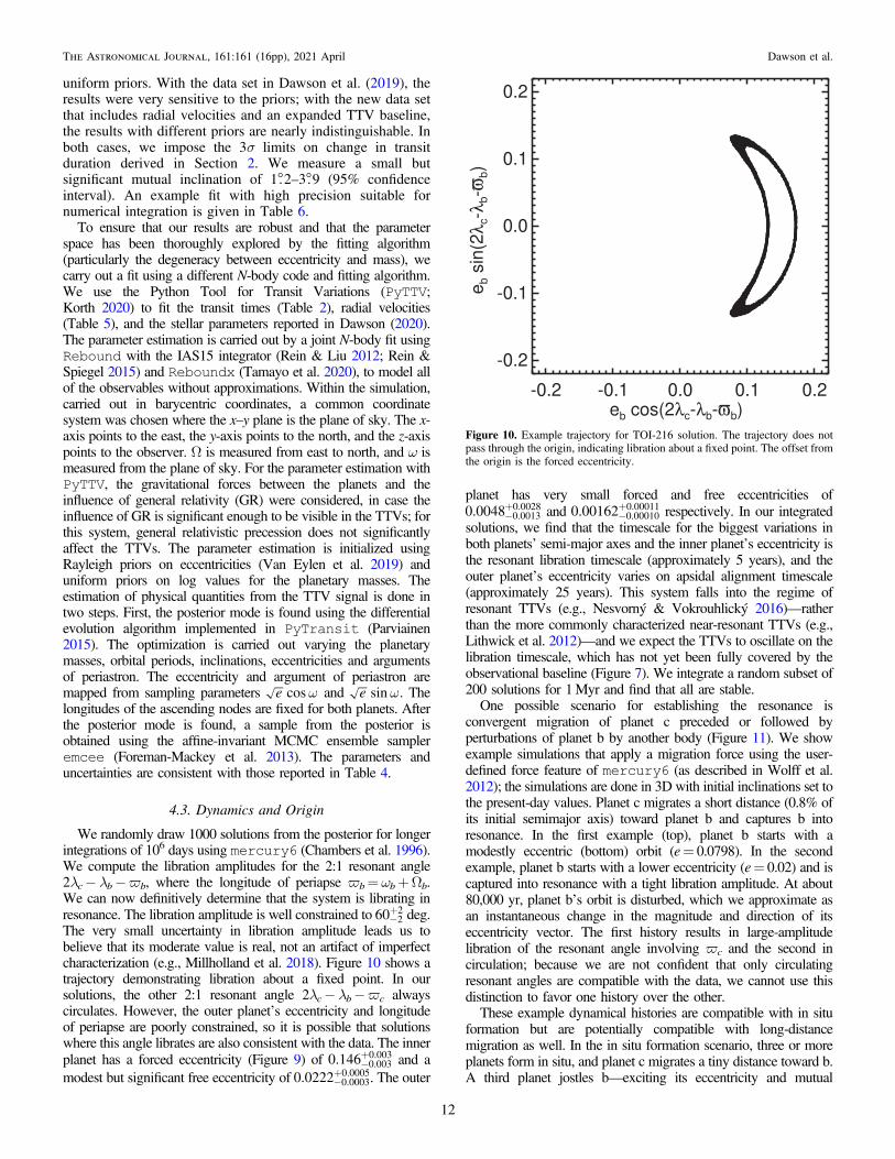
The very small uncertainty in libration amplitude leads us tobelieve that its moderate value is real, not an artifact of imperfectcharacterization (e.g., Millholland et al. 2018). Figure 10 shows atrajectory demonstrating libration about a fixed point. In oursolutions, the other 2:1 resonant angle 2λc− λb−ϖc alwayscirculates. However, the outer planet’s eccentricity and longitudeof periapse are poorly constrained, so it is possible that solutionswhere this angle librates are also consistent with the data. The innerplanet has a forced eccentricity (Figure 9) of -

+0.146 0.0030.003 and a

modest but significant free eccentricity of -+0.0222 0.0003

0.0005. The outer

planet has very small forced and free eccentricities of-+0.0048 0.0013

0.0028 and -+0.00162 0.00010

0.00011 respectively. In our integratedsolutions, we find that the timescale for the biggest variations inboth planets’ semi-major axes and the inner planet’s eccentricity isthe resonant libration timescale (approximately 5 years), and theouter planet’s eccentricity varies on apsidal alignment timescale(approximately 25 years). This system falls into the regime ofresonant TTVs (e.g., Nesvorný & Vokrouhlický 2016)—ratherthan the more commonly characterized near-resonant TTVs (e.g.,Lithwick et al. 2012)—and we expect the TTVs to oscillate on thelibration timescale, which has not yet been fully covered by theobservational baseline (Figure 7). We integrate a random subset of200 solutions for 1Myr and find that all are stable.One possible scenario for establishing the resonance is

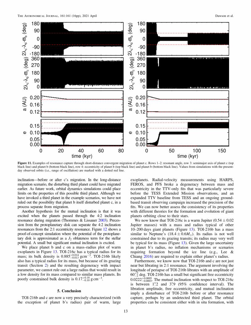
convergent migration of planet c preceded or followed byperturbations of planet b by another body (Figure 11). We showexample simulations that apply a migration force using the user-defined force feature of mercury6 (as described in Wolff et al.2012); the simulations are done in 3D with initial inclinations set tothe present-day values. Planet c migrates a short distance (0.8% ofits initial semimajor axis) toward planet b and captures b intoresonance. In the first example (top), planet b starts with amodestly eccentric (bottom) orbit (e= 0.0798). In the secondexample, planet b starts with a lower eccentricity (e= 0.02) and iscaptured into resonance with a tight libration amplitude. At about80,000 yr, planet b’s orbit is disturbed, which we approximate asan instantaneous change in the magnitude and direction of itseccentricity vector. The first history results in large-amplitudelibration of the resonant angle involving ϖc and the second incirculation; because we are not confident that only circulatingresonant angles are compatible with the data, we cannot use thisdistinction to favor one history over the other.These example dynamical histories are compatible with in situ

formation but are potentially compatible with long-distancemigration as well. In the in situ formation scenario, three or moreplanets form in situ, and planet c migrates a tiny distance toward b.A third planet jostles b—exciting its eccentricity and mutual

Figure 10. Example trajectory for TOI-216 solution. The trajectory does notpass through the origin, indicating libration about a fixed point. The offset fromthe origin is the forced eccentricity.

12

The Astronomical Journal, 161:161 (16pp), 2021 April Dawson et al.

inclination—before or after c’s migration. In the long-distancemigration scenario, the disturbing third planet could have migratedearlier. As future work, orbital dynamics simulations could placelimits on the properties of this possible third planet. Although wehave invoked a third planet in the example scenarios, we have notruled out the possibility that planet b itself disturbed planet c, in aprocess separate from migration.

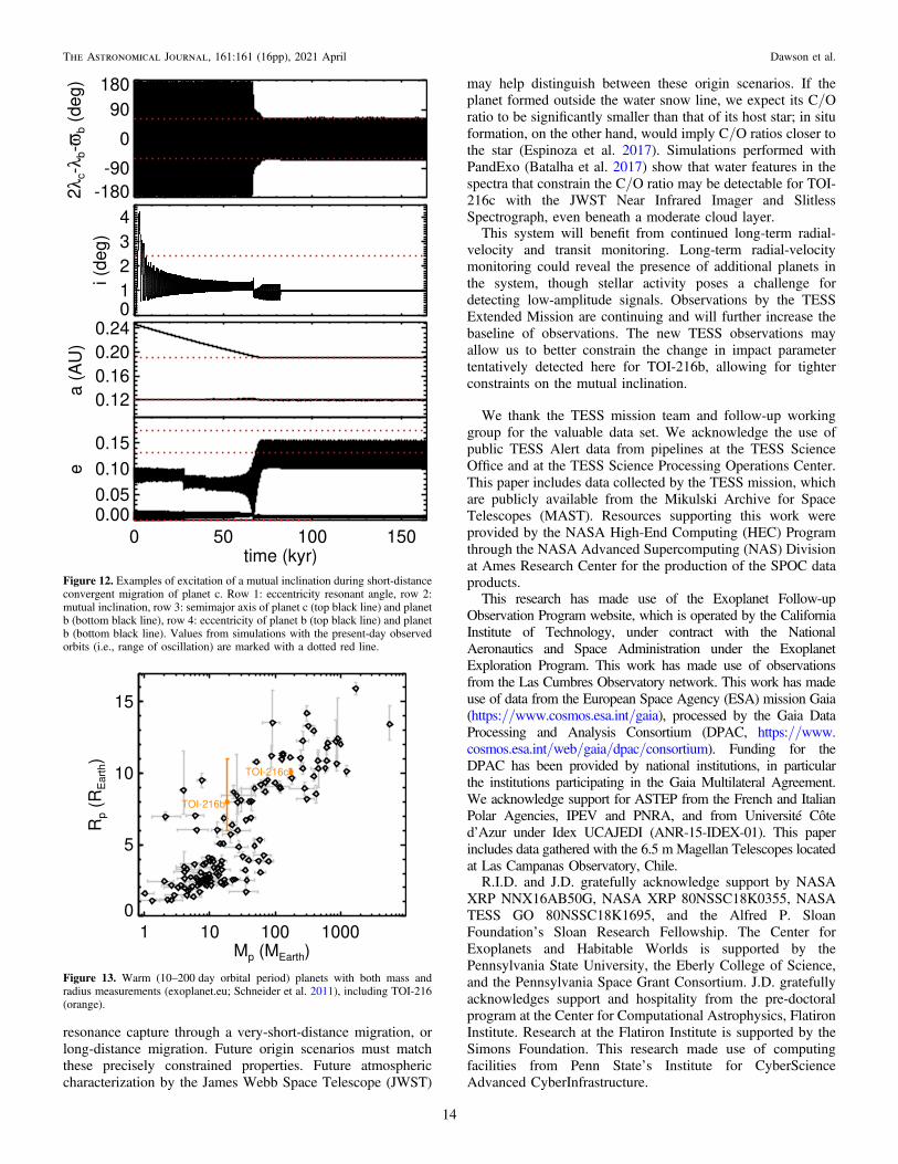
Another hypothesis for the mutual inclination is that it wasexcited when the planets passed through the 4:2 inclinationresonance during migration (Thommes & Lissauer 2003). Preces-sion from the protoplanetary disk can separate the 4:2 inclinationresonances from the 2:1 eccentricity resonance. Figure 12 shows aproof-of-concept simulation where the potential of the protoplane-tary disk is approximated as a J2 oblateness term for the stellarpotential. A small but significant mutual inclination is excited.

We place planet b and c on a mass–radius plot of warmexoplanets in Figure 13. TOI-216c has a typical radius for itsmass; its bulk density is -

+ -0.885 gcm0.0130.014 3. TOI-216b likely

also has a typical radius for its mass, but because of its grazingtransit (Section 2) and the resulting degeneracy with impactparameter, we cannot rule out a large radius that would result ina low density for its mass compared to similar mass planets. Itspoorly constrained bulk density is -

+ -0.17 g cm0.100.18 3.

5. Conclusion

TOI-216b and c are now a very precisely characterized (withthe exception of planet b’s radius) pair of warm, large

exoplanets. Radial-velocity measurements using HARPS,FEROS, and PFS broke a degeneracy between mass andeccentricity in the TTV-only fits that was particularly severebefore the TESS Extended Mission observations, and anexpanded TTV baseline from TESS and an ongoing ground-based transit observing campaign increased the precision of thefits. We can now better assess the consistency of its propertieswith different theories for the formation and evolution of giantplanets orbiting close to their stars.We now know that TOI-216c is a warm Jupiter (0.54± 0.02

Jupiter masses) with a mass and radius typical of other10–200 days giant planets (Figure 13). TOI-216b has a masssimilar to Neptune’s (18.4± 0.6M⊕). Its radius is not wellconstrained due to its grazing transits; its radius may very wellbe typical for its mass (Figure 13). Given the large uncertaintyin planet b’s radius, no inflation mechanisms or scenariosrequiring formation beyond the ice line (e.g., Lee &Chiang 2016) are required to explain either planet’s radius.Furthermore, we know now that TOI-216b and c are not just

near but librating in 2:1 resonance. The argument involving thelongitude of periapse of TOI-216b librates with an amplitude of

-+60 2

2 deg. TOI-216b has a small but significant free eccentricity

-+0.0222 0.0003

0.0005. The mutual inclination with respect to TOI-216cis between 1°.2 and 3°.9 (95% confidence interval). Thelibration amplitude, free eccentricity, and mutual inclinationimply a disturbance of TOI-216b before or after resonancecapture, perhaps by an undetected third planet. The orbitalproperties can be consistent either with in situ formation, with

Figure 11. Examples of resonance capture through short-distance convergent migration of planet c. Rows 1–2: resonant angle, row 3: semimajor axis of planet c (topblack line) and planet b (bottom black line), row 4: eccentricity of planet b (top black line) and planet b (bottom black line). Values from simulations with the present-day observed orbits (i.e., range of oscillation) are marked with a dotted red line.

13

The Astronomical Journal, 161:161 (16pp), 2021 April Dawson et al.

resonance capture through a very-short-distance migration, orlong-distance migration. Future origin scenarios must matchthese precisely constrained properties. Future atmosphericcharacterization by the James Webb Space Telescope (JWST)

may help distinguish between these origin scenarios. If theplanet formed outside the water snow line, we expect its C/Oratio to be significantly smaller than that of its host star; in situformation, on the other hand, would imply C/O ratios closer tothe star (Espinoza et al. 2017). Simulations performed withPandExo (Batalha et al. 2017) show that water features in thespectra that constrain the C/O ratio may be detectable for TOI-216c with the JWST Near Infrared Imager and SlitlessSpectrograph, even beneath a moderate cloud layer.This system will benefit from continued long-term radial-

velocity and transit monitoring. Long-term radial-velocitymonitoring could reveal the presence of additional planets inthe system, though stellar activity poses a challenge fordetecting low-amplitude signals. Observations by the TESSExtended Mission are continuing and will further increase thebaseline of observations. The new TESS observations mayallow us to better constrain the change in impact parametertentatively detected here for TOI-216b, allowing for tighterconstraints on the mutual inclination.

We thank the TESS mission team and follow-up workinggroup for the valuable data set. We acknowledge the use ofpublic TESS Alert data from pipelines at the TESS ScienceOffice and at the TESS Science Processing Operations Center.This paper includes data collected by the TESS mission, whichare publicly available from the Mikulski Archive for SpaceTelescopes (MAST). Resources supporting this work wereprovided by the NASA High-End Computing (HEC) Programthrough the NASA Advanced Supercomputing (NAS) Divisionat Ames Research Center for the production of the SPOC dataproducts.This research has made use of the Exoplanet Follow-up

Observation Program website, which is operated by the CaliforniaInstitute of Technology, under contract with the NationalAeronautics and Space Administration under the ExoplanetExploration Program. This work has made use of observationsfrom the Las Cumbres Observatory network. This work has madeuse of data from the European Space Agency (ESA) mission Gaia(https://www.cosmos.esa.int/gaia), processed by the Gaia DataProcessing and Analysis Consortium (DPAC, https://www.cosmos.esa.int/web/gaia/dpac/consortium). Funding for theDPAC has been provided by national institutions, in particularthe institutions participating in the Gaia Multilateral Agreement.We acknowledge support for ASTEP from the French and ItalianPolar Agencies, IPEV and PNRA, and from Université Côted’Azur under Idex UCAJEDI (ANR-15-IDEX-01). This paperincludes data gathered with the 6.5 m Magellan Telescopes locatedat Las Campanas Observatory, Chile.R.I.D. and J.D. gratefully acknowledge support by NASA

XRP NNX16AB50G, NASA XRP 80NSSC18K0355, NASATESS GO 80NSSC18K1695, and the Alfred P. SloanFoundation’s Sloan Research Fellowship. The Center forExoplanets and Habitable Worlds is supported by thePennsylvania State University, the Eberly College of Science,and the Pennsylvania Space Grant Consortium. J.D. gratefullyacknowledges support and hospitality from the pre-doctoralprogram at the Center for Computational Astrophysics, FlatironInstitute. Research at the Flatiron Institute is supported by theSimons Foundation. This research made use of computingfacilities from Penn State’s Institute for CyberScienceAdvanced CyberInfrastructure.

Figure 12. Examples of excitation of a mutual inclination during short-distanceconvergent migration of planet c. Row 1: eccentricity resonant angle, row 2:mutual inclination, row 3: semimajor axis of planet c (top black line) and planetb (bottom black line), row 4: eccentricity of planet b (top black line) and planetb (bottom black line). Values from simulations with the present-day observedorbits (i.e., range of oscillation) are marked with a dotted red line.

Figure 13. Warm (10–200 day orbital period) planets with both mass andradius measurements (exoplanet.eu; Schneider et al. 2011), including TOI-216(orange).

14

The Astronomical Journal, 161:161 (16pp), 2021 April Dawson et al.

We thank Caleb Cañas and David Nesvorný for helpfulcomments and discussions. We thank the referee for a helpfulreport.

R.B. acknowledges support from FONDECYT Project11200751 and from CORFO project No. 14ENI2-26865. A.J., R.B., and M.H. acknowledge support from projectIC120009 “Millennium Institute of Astrophysics (MAS)” ofthe Millennium Science Initiative, Chilean Ministry ofEconomy. A.J. acknowledges additional support from FON-DECYT project 1171208. This research received funding fromthe European Research Council (ERC) under the EuropeanUnion’s Horizon 2020 research and innovation program(grant agreement No. 803193/BEBOP), and from the Scienceand Technology Facilities Council (STFC; grant No. ST/S00193X/1). J. Korth acknowledges support by DFG grantsPA525/19-1 within the DFG Schwerpunkt SPP 1992, Explor-ing the Diversity of Extrasolar Planets. Part of this research wascarried out at the Jet Propulsion Laboratory, California Instituteof Technology, under a contract with the National Aeronauticsand Space Administration (NASA).

Software: mpfit (Markwardt 2009), TAP (Gazak et al. 2012),Tapir (Jensen 2013), TESS pipeline (Jenkins et al. 2016;Twicken et al. 2018; Li et al. 2019), AstroImageJ (Collinset al. 2017), exoplanet (Foreman-Mackey et al. 2019),astropy (Astropy Collaboration et al. 2013, 2018), cel-erite (Foreman-Mackey et al. 2017; Foreman-Mackey 2018),starry (Luger et al. 2019), pymc3 (Salvatier et al. 2016),theano (Theano Development Team 2016), ceres (Brahmet al. 2017), PyTTV, PyTransit (Parviainen 2015), emcee(Foreman-Mackey et al. 2013), eleanor (Feinstein et al.2019).

ORCID iDs

Rebekah I. Dawson https://orcid.org/0000-0001-9677-1296Chelsea X. Huang https://orcid.org/0000-0003-0918-7484Rafael Brahm https://orcid.org/0000-0002-9158-7315Karen A. Collins https://orcid.org/0000-0001-6588-9574Melissa J. Hobson https://orcid.org/0000-0002-5945-7975Jiayin Dong https://orcid.org/0000-0002-3610-6953Trifon Trifonov https://orcid.org/0000-0002-0236-775XR. Paul Butler https://orcid.org/0000-0003-1305-3761Mauro Barbieri https://orcid.org/0000-0001-8362-3462Kevin I. Collins https://orcid.org/0000-0003-2781-3207Dennis M. Conti https://orcid.org/0000-0003-2239-0567Jeffrey D. Crane https://orcid.org/0000-0002-5226-787XNicolas Crouzet https://orcid.org/0000-0001-7866-8738Néstor Espinoza https://orcid.org/0000-0001-9513-1449Tianjun Gan https://orcid.org/0000-0002-4503-9705Tristan Guillot https://orcid.org/0000-0002-7188-8428Thomas Henning https://orcid.org/0000-0002-1493-300XEric L. N. Jensen https://orcid.org/0000-0002-4625-7333Djamel Mékarnia https://orcid.org/0000-0001-5000-7292Gordon Myers https://orcid.org/0000-0002-9810-0506Paula Sarkis https://orcid.org/0000-0001-8128-3126Stephen Shectman https://orcid.org/0000-0002-8681-6136François-Xavier Schmider https://orcid.org/0000-0003-3914-3546Avi Shporer https://orcid.org/0000-0002-1836-3120Chris Stockdale https://orcid.org/0000-0003-2163-1437Amaury H. M. J. Triaud https://orcid.org/0000-0002-5510-8751Carl Ziegler https://orcid.org/0000-0002-0619-7639

G. Ricker https://orcid.org/0000-0003-2058-6662R. Vanderspek https://orcid.org/0000-0001-6763-6562David W. Latham https://orcid.org/0000-0001-9911-7388J. Winn https://orcid.org/0000-0002-4265-047XJon M. Jenkins https://orcid.org/0000-0002-4715-9460L. G. Bouma https://orcid.org/0000-0002-0514-5538Jennifer A. Burt https://orcid.org/0000-0002-0040-6815David Charbonneau https://orcid.org/0000-0002-9003-484XBrian McLean https://orcid.org/0000-0002-8058-643XMark E. Rose https://orcid.org/0000-0003-4724-745XAndrew Vanderburg https://orcid.org/0000-0001-7246-5438

References

Agol, E., Steffen, J., Sari, R., & Clarkson, W. 2005, MNRAS, 359, 567Anderson, K. R., Lai, D., & Pu, B. 2020, MNRAS, 491, 1369Anglada-Escudé, G., López-Morales, M., & Chambers, J. E. 2010, ApJ,

709, 168Astropy Collaboration, Price-Whelan, A. M., Sipőcz, B. M., et al. 2018, AJ,

156, 123Astropy Collaboration, Robitaille, T. P., Tollerud, E. J., et al. 2013, A&A,

558, A33Batalha, N. E., Mandell, A., Pontoppidan, K., et al. 2017, PASP, 129, 064501Boisse, I., Moutou, C., Vidal-Madjar, A., et al. 2009, A&A, 495, 959Brahm, R., Espinoza, N., Jordán, A., et al. 2019, AJ, 158, 45Brahm, R., Jordán, A., & Espinoza, N. 2017, PASP, 129, 034002Brown, T. M., Baliber, N., Bianco, F. B., et al. 2013, PASP, 125, 1031Butler, R. P., Marcy, G. W., Williams, E., et al. 1996, PASP, 108, 500Canto Martins, B. L., Gomes, R. L., Messias, Y. S., et al. 2020, ApJS, 250, 20Carter, J. A., & Winn, J. N. 2009, ApJ, 704, 51Chambers, J. E., Wetherill, G. W., & Boss, A. P. 1996, Icar, 119, 261Choksi, N., & Chiang, E. 2020, MNRAS, in pressCollins, K. A., Kielkopf, J. F., Stassun, K. G., & Hessman, F. V. 2017, AJ,

153, 77Crane, J. D., Shectman, S. A., & Butler, R. P. 2006, Proc. SPIE, 6269, 626931Crane, J. D., Shectman, S. A., Butler, R. P., et al. 2010, Proc. SPIE, 7735,

773553Crane, J. D., Shectman, S. A., Butler, R. P., Thompson, I. B., & Burley, G. S.

2008, Proc. SPIE, 7014, 701479Cumming, A. 2004, MNRAS, 354, 1165Cumming, A., Marcy, G. W., & Butler, R. P. 1999, ApJ, 526, 890Dawson, R. I. 2020, AJ, 159, 223Dawson, R. I., Huang, C. X., Lissauer, J. J., et al. 2019, AJ, 158, 65Dawson, R. I., & Johnson, J. A. 2012, ApJ, 756, 122Dawson, R. I., & Johnson, J. A. 2018, ARA&A, 56, 175Dawson, R. I., Johnson, J. A., Fabrycky, D. C., et al. 2014, ApJ, 791, 89Deck, K. M., & Agol, E. 2015, ApJ, 802, 116Dong, R., & Dawson, R. 2016, ApJ, 825, 77Edelson, R. A., & Krolik, J. H. 1988, ApJ, 333, 646Espinoza, N., Fortney, J. J., Miguel, Y., Thorngren, D., & Murray-Clay, R.

2017, ApJ, 838, L9Feinstein, A. D., Montet, B. T., Foreman-Mackey, D., et al. 2019, PASP, 131,

094502Foreman-Mackey, D. 2018, RNAAS, 2, 31Foreman-Mackey, D., Agol, E., Ambikasaran, S., & Angus, R. 2017, AJ,

154, 220Foreman-Mackey, D., Czekala, I., Luger, R., et al. 2019, dfm/exoplanet:

exoplanet v0.2.1, Zenodo, doi:10.5281/zenodo.3462740Foreman-Mackey, D., Hogg, D. W., Lang, D., & Goodman, J. 2013, PASP,

125, 306Frelikh, R., Jang, H., Murray-Clay, R. A., & Petrovich, C. 2019, ApJ, 884, L47Gazak, J. Z., Johnson, J. A., Tonry, J., et al. 2012, AdAst, 2012, 697967Huang, C., Wu, Y., & Triaud, A. H. M. J. 2016, ApJ, 825, 98Jenkins, J. M., Caldwell, D. A., & Borucki, W. J. 2002, ApJ, 564, 495Jenkins, J. M., Caldwell, D. A., Chandrasekaran, H., et al. 2010, ApJ, 713, L87Jenkins, J. M., Twicken, J. D., McCauliff, S., et al. 2016, Proc. SPIE, 9913,

99133EJensen, E. 2013, Tapir: A Web Interface for Transit/Eclipse Observability,

Astrophysics Source Code Library, ascl:1306.007Jordán, A., Brahm, R., Espinoza, N., et al. 2020, AJ, 159, 145

15

The Astronomical Journal, 161:161 (16pp), 2021 April Dawson et al.

Kaufer, A., Stahl, O., Tubbesing, S., et al. 1999, Msngr, 95, 8Kipping, D., Nesvorný, D., Hartman, J., et al. 2019, MNRAS, 486, 4980Kipping, D. M. 2013, MNRAS, 435, 2152Korth, J. 2020, PhD thesis, Univ. Cologne, https://kups.ub.uni-koeln.de/

11289/Kürster, M., Trifonov, T., Reffert, S., Kostogryz, N. M., & Rodler, F. 2015,

A&A, 577, A103Lee, E. J., & Chiang, E. 2016, ApJ, 817, 90Lee, M. H., & Peale, S. J. 2002, ApJ, 567, 596Li, J., Tenenbaum, P., Twicken, J. D., et al. 2019, PASP, 131, 024506Lithwick, Y., & Naoz, S. 2011, ApJ, 742, 94Lithwick, Y., Xie, J., & Wu, Y. 2012, ApJ, 761, 122Luger, R., Agol, E., Foreman-Mackey, D., et al. 2019, AJ, 157, 64MacDonald, M. G., & Dawson, R. I. 2018, AJ, 156, 228Mandel, K., & Agol, E. 2002, ApJ, 580, L171Markwardt, C. B. 2009, in ASP Conf. Ser. 411, Astronomical Data Analysis

Software and Systems XVIII, ed. D. A. Bohlender, D. Durand, & P. Dowler(San Francisco, CA: ASP), 251

Mayor, M., Pepe, F., Queloz, D., et al. 2003, Msngr, 114, 20McCully, C., Volgenau, N. H., Harbeck, D.-R., et al. 2018, Proc. SPIE, 10707,

107070KMcQuillan, A., Mazeh, T., & Aigrain, S. 2014, ApJS, 211, 24

Millholland, S., Laughlin, G., Teske, J., et al. 2018, AJ, 155, 106Morrison, S. J., Dawson, R. I., & MacDonald, M. 2020, ApJ, 904, 157Mustill, A. J., Davies, M. B., & Johansen, A. 2015, ApJ, 808, 14Nesvorný, D., & Vokrouhlický, D. 2016, ApJ, 823, 72Parviainen, H. 2015, MNRAS, 450, 3233Rein, H., & Liu, S. F. 2012, A&A, 537, A128Rein, H., & Spiegel, D. S. 2015, MNRAS, 446, 1424Salvatier, J., Wiecki, T. V., & Fonnesbeck, C. 2016, PeerJ Computer Science,

2, e55Schneider, J., Dedieu, C., Le Sidaner, P., Savalle, R., & Zolotukhin, I. 2011,

A&A, 532, A79Smith, J. C., Stumpe, M. C., Van Cleve, J. E., et al. 2012, PASP, 124, 1000Stumpe, M. C., Smith, J. C., Catanzarite, J. H., et al. 2014, PASP, 126, 100Tamayo, D., Rein, H., Shi, P., & Hernand ez, D. M. 2020, MNRAS, 491,

2885Theano Development Team 2016, arXiv:1605.02688Thommes, E. W., & Lissauer, J. J. 2003, ApJ, 597, 566Twicken, J. D., Catanzarite, J. H., Clarke, B. D., et al. 2018, PASP, 130,

064502Van Eylen, V., Albrecht, S., Huang, X., et al. 2019, AJ, 157, 61Wolff, S., Dawson, R. I., & Murray-Clay, R. A. 2012, ApJ, 746, 171Zechmeister, M., & Kürster, M. 2009, A&A, 496, 577

16

The Astronomical Journal, 161:161 (16pp), 2021 April Dawson et al.