Radial Velocity

Christophe LovisUniversite de Geneve

Debra A. FischerYale University

The radial velocity technique was utilized to make the first exoplanet discoveries andcontinues to play a major role in the discovery and characterization of exoplanetary systems. Inthis chapter we describe how the technique works, and the current precision and limitations. Wethen review its major successes in the field of exoplanets. With more than 250 planet detections,it is the most prolific technique to date and has led to many milestone discoveries, such ashot Jupiters, multi-planet systems, transiting planets around bright stars, the planet-metallicitycorrelation, planets around M dwarfs and intermediate-mass stars, and recently, the emergenceof a population of low-mass planets: ice giants and super-Earths. In the near future radialvelocities are expected to systematically explore the domain of telluric and icy planets downto a few Earth masses close to the habitable zone of their parent star. They will also be usedto provide the necessary follow-up observations of transiting candidates detected by spacemissions. Finally, we also note alternative radial velocity techniques that may play an importantrole in the future.

1. INTRODUCTION

Since the end of the XIXth century, radial velocities havebeen at the heart of many developments and advances in as-trophysics. In 1888, Vogel at Potsdam used photography todemonstrate Christian Dopplers theory (in 1842) that starsin motion along our line of site would exhibit a change incolor. This color change, or wavelength shift, is commonlyknown as a Doppler shift and it has been a powerful toolover the past century, used to measure stellar kinematics, todetermine orbital parameters for stellar binary systems, andto identify stellar pulsations. By 1953, radial velocities hadbeen compiled for more than 15,000 stars in the GeneralCatalogue of Stellar Radial Velocities (Wilson 1953) witha typical precision of 750 m s−1, not the precision that istypically associated with planet-hunting. However, at thattime, Otto Struve proposed that high precision stellar radialvelocity work could be used to search for planets orbitingnearby stars. He made the remarkable assertion that Jupiter-like planets could reside as close as 0.02 AU from their hoststars. Furthermore, he noted that if such close-in planetswere ten times the mass of our Jupiter, the reflex stellar ve-locity for an edge-on orbit would be about 2 km s−1 anddetectable with 1950’s Doppler precision (Struve 1952).

Two decades later, Griffin & Griffin (1973) identified akey weakness in radial velocity techniques of the day; thestellar spectrum was measured with respect to an emissionspectrum. However, the calibrating lamps (typically tho-rium argon) did not illuminate the slit and spectrometercollimator in the same way as the star. Griffin & Griffinoutlined a strategy for improving Doppler precision to a re-markable 10 m s−1 by differentially measuring stellar line

shifts with resepct to telluric lines. Assuming that telluriclines are at rest relative to the spectrometer, these absorp-tion lines would trace the stellar light path and illuminatethe optics in the same way and at the same time as the star.Although Griffin & Griffin did not obtain this high preci-sion, they had highlighted some of the key challenges thatcurrent techniques have overcome.

By 1979, Gordon Walker and Bruce Campbell had a ver-sion of telluric lines in a bottle: a glass cell containing hy-drogen fluoride that was inserted in the light path at theCFHT (Campbell & Walker 1979). Like telluric lines, theHF absorption lines were imprinted in the stellar spectrumand provided a precise wavelength solution spanning about50 A. The spectrum was recorded with a photon-countingReticon photodiode array. Working from 1980 to 1992, theymonitored 17 main sequence stars and 4 subgiant stars andachieved the unprecedented precision of 15 m s−1. Unfor-tunately, because of the small sample size, no planets werefound. However, upper limits were set onM sin i for orbitalperiods out to 15 years for the 21 stars that they observed(Walker et al. 1995).

Cross-correlation speedometers were also used to mea-sure radial velocities relative to a physical template. In1989, an object with M sin i of 11 MJup was discoveredin an 84-day orbit around HD 114762 (Latham et al. 1989).The velocity amplitude of the star was 600 m s−1 and al-though the single measurement radial velocity precisionwas only about 400 m s−1, hundreds of observations effec-tively beat down the noise to permit this first detection of asubstellar object.

In 1993, the ELODIE spectrometer was commissionedon the 1.93-m telescope at Observatoire de Haute-Provence

1

(OHP, France). To bypass the problem of different lightpaths for stellar and reference lamp sources described byGriffin & Griffin (1973), two side-by-side fibers were usedat ELODIE. Starlight passed through one fiber and lightfrom a thorium argon lamp illuminated the second fiber.The calibration and stellar spectrum were offset in thecross-dispersion direction on the CCD detector and a ve-locity precision of about 13 m s−1 enabled the detection ofa Jupiter-like planet orbiting 51 Pegasi (Mayor & Queloz1995). In a parallel effort to achieve high Doppler preci-sion, a glass cell containing iodine vapor was employed byMarcy & Butler (1995) to confirm the detection of a plane-tary companion around 51 Peg b. Both Doppler techniqueshave continued to show remarkable improvements in preci-sion, and have ushered in an era of exoplanet discoveries.

2. DESCRIPTION OF THE TECHNIQUE

2.1. Radial Velocity Signature of Keplerian Motion

The aim of this section is to derive the radial velocityequation, i.e. the relation between the position of a bodyon its orbit and its radial velocity, in the case of Keplerianmotion. We present here a related approach to Chapter 2on Keplerian Dynamics. As shown there, the solutions ofthe gravitational two-body problem describe elliptical orbitsaround the common center of mass if the system is bound,with the center of mass located at a focus of the ellipses.Energy and angular momentum are constants of the motion.The semi-major axis of the first body orbit around the centerof mass a1 is related to the semi-major axis of the relativeorbit a through:

a1 =m2

m1 +m2a , (1)

where m1 and m2 are the masses of the bodies.In polar coordinates, the equation of the ellipse described

by the first body around the center of mass reads:

r1 =a1(1− e2)1 + e cos f

=m2

m1 +m2· a(1− e2)

1 + e cos f, (2)

where r1 is the distance of the first body from the centerof mass, e is the eccentricity and f is the true anomaly, i.e.the angle between the periastron direction and the positionon the orbit, as measured from the center of mass. The trueanomaly as a function of time can be computed via Kepler’sequation, which cannot be solved analytically, and thereforenumerical methods have to be used (see Chapter 2).

In this section we want to obtain the relation betweenposition on the orbit, given by f , and orbital velocity. Morespecifically, since our observable will be the radial veloc-ity of the object, we have to project the orbital velocity ontothe line of sight linking the observer to the system. In Carte-sian coordinates, with the x-axis pointing in the periastrondirection and the origin at the center of mass, the positionand velocity vectors are given by:

r1 =(r1 cos fr1 sin f

), (3)

r1 =(r1 cos f − r1f sin fr1 sin f + r1f cos f

). (4)

We now need to express r1 and f as a function of f inorder to obtain the velocity as a function of f alone. In afirst step, we differentiate Eq. 2 to obtain r1:

r1 =a1e(1− e2)f sin f

(1 + e cos f)2=er2

1 f sin fa1(1− e2)

. (5)

Replacing r1 in Eq. 4, we obtain after some algebra:

r1 =r21 f

a1(1− e2)

(− sin f

cos f + e

)(6)

=h1

m1a1(1− e2)

(− sin f

cos f + e

), (7)

where h1 = m1r21 f is the angular momentum of the first

body, which is a constant of the motion. It can be ex-pressed as a function of the ellipse parameters a and e as(see Chap. 2):

h1 =m2

m1 +m2h =

√Gm2

1m42a(1− e2)

(m1 +m2)3. (8)

Substituting h1 in Eq. 6, we finally obtain:

r1 =

√Gm2

2

m1 +m2

1a(1− e2)

(− sin f

cos f + e

). (9)

As a final step, the velocity vector has to be projectedonto the line of sight of the observer. We define the inclina-tion angle i of the system as the angle between the orbitalplane and the plane of the sky (i.e. the perpendicular to theline of sight). We further define the argument of periastronω as the angle between the line of nodes and the periastrondirection (see Fig. 5 of Chapter 2 for an overview of the ge-ometry). In a Cartesian coordinate system with x- and y-axes in the orbital plane as before and the z-axis perpendic-ular to them, the unit vector of the line of sight k is givenby:

k =

sinω sin icosω sin i

cos i

. (10)

The radial velocity equation is obtained by projecting thevelocity vector on k:

vr,1 = r1 · k

=

√G

(m1+m2)a(1−e2)m2 sin i

· (cos (ω + f) + e cosω) .

(11)

2

This is the fundamental equation relating the radial ve-locity to the position on the orbit. From there we can de-rive the radial velocity semi-amplitude K = (vr,max −vr,min)/2:

K1 =

√G

(1−e2)m2 sin i (m1+m2)−1/2 a−1/2 . (12)

It is useful to express this formula in more practicalunits:

K1 =28.4329 m s−1

√1−e2

m2 sin iMJup

(m1+m2

M�

)−1/2 ( a

1 AU

)−1/2

.

(13)Alternatively, one can use Kepler’s third law to replace

the semi-major axis a with the orbital period P :

K1 =28.4329 m s−1

√1−e2

m2 sin iMJup

(m1+m2

M�

)−2/3(P

1 yr

)−1/3

.

(14)In the exoplanet case, only the radial velocity of the

parent star is in general observable, because the planet-to-star flux ratio is so small (.10−5). Radial velocity ob-servations covering all orbital phases are able to measurethe orbital period P , the eccentricity e and the RV semi-amplitude K1. From these observables, the so-called ’min-imum mass’ m2 sin i can be computed, provided the totalmass of the system m1 + m2 is known. In practice, plan-etary masses are usually negligible compared to the massof the parent star. The stellar mass can be obtained indi-rectly via spectroscopic analysis, photometry, parallax mea-surements and comparison with stellar evolutionary mod-els. For bright, main-sequence FGKM stars, Hipparcosdata and precise spectral synthesis make it possible to esti-mate stellar masses to ∼5%. Another, more precise way ofobtaining stellar masses is via asteroseismic observations,since stellar pulsation frequencies are directly related to thebasic stellar parameters such as mass, radius and chemicalcomposition.

The unknown inclination angle i prevents us from mea-suring the true mass of the companion m2. While this isan important limitation of the RV technique for individualsystems, this fact does not have a large impact on statisti-cal studies of exoplanet populations. Because inclinationangles are randomly distributed in space, angles close to90◦ (edge-on systems) are much more frequent than pole-on configurations. Indeed, the distribution function for i isgiven by f(i)di = sin i di. As a consequence, the averagevalue of sin i is equal to π/4 (0.79). Moreover, the a prioriprobability that sin i is larger than 0.5 is 87%.

Eq. 13 gives RV semi-amplitudes as a function of or-bital parameters. Table 2.1 lists a few typical examples forplanets with different masses and semi-major axes orbitinga solar-mass star. As one can see, the search for exoplan-ets with the RV technique requires a precision of at least

Table 1: Radial velocity signals for different kinds of plan-ets orbiting a solar-mass star.

Planet a (AU) K1 (m s−1)Jupiter 0.1 89.8Jupiter 1.0 28.4Jupiter 5.0 12.7Neptune 0.1 4.8Neptune 1.0 1.5Super-Earth (5 M⊕) 0.1 1.4Super-Earth (5 M⊕) 1.0 0.45Earth 0.1 0.28Earth 1.0 0.09

∼30 m s−1 to detect giant planets. Towards lower masses,a precision of ∼1 m s−1 is necessary to access the domainof Neptune-like planets and super-Earths, while measure-ments at ∼0.1 m s−1 would be able to reveal the Earth. It isinteresting to consider here planet searches around lower-mass stars, since the Doppler signal increases as 1/

√m1 at

constant semi-major axis. For a 0.1-M� M dwarf, all RVamplitudes given in Table 2.1 must be multiplied by 3. Con-sidering that the habitable zone around such stars may be asclose as 0.1 AU, an Earth-like planet would induce a RVsignal of 0.9 m s−1. While the gain is significant comparedto habitable Earths around FGK stars, it must be balancedby the intrinsic faintness of these stars, which makes it dif-ficult to obtain high enough a signal-to-noise ratio to reachthe required precision, even with 10-m telescopes.

2.2. Doppler Effect

The fundamental effect on which the radial velocitytechnique relies is the well-known Doppler effect. In flatspacetime (special relativity), an emitted photon of wave-length λ0 in the rest frame of the source will be detectedat a different wavelength λ by an observer moving with re-spect to the emitter, where λ is given by (Einstein 1905):

λ = λ0

1 + 1c k · v√

1− v2

c2

. (15)

In this equation, v is the velocity of the source relativeto the observer, k is the unit vector pointing from the ob-server to the source in the rest frame of the observer, and cis the speed of light in vacuum. As one can see, the Dopplershift mainly depends on the projection of the velocity vectoralong the line of sight, i.e. the radial velocity of the source.There is also a dependence on the magnitude of the velocityvector, which means that the transverse velocity also con-tributes to the Doppler shift. However, this relativistic effectis often negligible in practical applications where velocitiesremain small compared to the speed of light.

In the framework of general relativity, the curvature ofspacetime, giving rise to the so-called gravitational redshift,has to be taken into account in the derivation of the Dopplershift formula. Neglecting terms of order c−4 and higher, the

3

general-relativistic Doppler formula becomes, for an ob-server at zero gravitational potential (Lindegren & Dravins2003):

λ = λ0

1 + 1c k · v

1− Φc2 − v2

2c2

, (16)

where Φ is the Newtonian gravitational potential at thesource (Φ = GM/r at a distance r of a spherically-symmetric mass M ).

The Doppler effect, being a relation between wavelength(or frequency) of light and velocity of the emitter, opensthe possibility to measure the (radial) velocity of a star asa function of time, thereby permitting the detection of or-biting companions according to the equations given in theprevious section. In practice, the Doppler shift is mea-sured on the numerous spectral lines that are present instellar spectra. However, Earth-bound Doppler shift mea-surements must first be corrected from the effects of localmotions of the observer, i.e. Earth rotation and revolutionaround the Sun, before they can be used to study the be-haviour of the target star. The barycenter of the Solar Sys-tem represents the most obvious local rest frame to whichmeasurements should be referred. A corresponding suitablereference system centered on the Solar System barycen-ter, the International Celestial Reference System (ICRS),has been defined by the International Astronomical Union(IAU) and has become the standard reference system (Rick-man 2001). Based on Eq. 16, the transformation of mea-sured wavelengths at Earth to barycentric wavelengths iscalled ’barycentric correction’ and is given by:

λB = λobs

1 + 1c k · vobs

1− Φobsc2 −

v2obs

2c2

, (17)

where λB is the wavelength that would be measured in theICRS, λobs is the measured wavelength in the Earth-boundframe, k is the unit vector pointing from the observer to thesource in the ICRS, vobs is the velocity of the observer withrespect to the ICRS, and Φobs is the gravitational potentialat the observer.

The main term in this equation is of course the projec-tion of the observer velocity (in the ICRS) in the directionof the source at the time of the observation. It is made oftwo contributions: the Earth orbital velocity and the Earthrotational velocity at the observer’s location. These can becomputed using precise Solar System ephemerides such asthose developed by JPL (Standish 1990) or IMCCE (Fiengaet al. 2008). When aiming at radial velocity precisions of 1m s−1 or below, all input parameters must be known to highprecision and carefully checked. Target coordinates mustbe given in the ICRS, corrected from proper motions. Theobservatory clock must reliably give UT time, and ideallythe photon-weighted mid-exposure time should be used.Finally, the observatory coordinates and altitude must beknown precisely.

The relativistic term appearing in the denominator ofEq. 17 has a magnitude of a few m s−1 in velocity units and,

more importantly, exhibits variations at the level of only 0.1m s−1 over the year due to the eccentricity of Earth’s orbit.Therefore, if one is interested in radial velocity variationsat a precision not exceeding 0.1 m s−1, the relativistic termcan be neglected and Eq. 17 reduces to the familiar classicalexpression

λB = λobs

(1 +

1ck · vobs

). (18)

After correcting the laboratory wavelength scale to thebarycentric scale, the radial velocity of the source can fi-nally be obtained from the expression

λB = λ0

1 + 1c k · v∗

1− Φ∗c2 − v2

∗2c2

, (19)

where v∗ and Φ∗ are the source velocity and gravitationalpotential, respectively. Again, the relativistic term impliesthat it is in principle necessary to know the transverse ve-locity of the source to properly derive its radial velocity.However, if one is only interested in low-amplitude radialvelocity variations, such as those produced by exoplanets,the relativistic term can also be dropped, yielding the famil-iar expression for the radial velocity:

k · v∗ = cλB − λ0

λ0. (20)

We emphasize here that we are focusing on precise (i.e.reproducible), but not accurate (i.e. absolute), radial ve-locities. Indeed, obtaining absolute stellar radial velocitiesthrough the Doppler effect is a very difficult task due tomany perturbing systematic effects, such as: gravitationalredshift, convective blueshifts of stellar lines, line asymme-tries, instrumental and wavelength calibration systematics,etc. These effects introduce unknown offsets on the mea-sured radial velocities that may add up to ∼1 km s−1 forsolar-type stars and high-resolution spectrographs. How-ever, since they remain essentially constant with time, theydo not prevent the detection of low-amplitude radial veloc-ity signals. The reader is referred to Lindegren & Dravins(2003) for a stringent definition of the concept of radial ve-locity and an in-depth discussion of all relevant perturbingeffects.

2.3. High-Resolution Spectra of Cool Stars

Stellar Doppler shift measurements rely on the presenceof spectral features in the emergent spectrum. Since starsemit most of their electromagnetic energy between the UVand mid-IR domains, and since the UV and mid-IR do-mains themselves are not accessible from the ground, ra-dial velocity work has always focused on spectral lines inthe visible and near-IR regions. Stellar spectra vary widelyacross the different regions of the Hertzsprung-Russell di-agram. Perhaps the single most relevant physical param-eter that controls their general properties is the effectivetemperature of the stellar photosphere. On the hot side(Teff & 10,000 K), all chemical elements are at least partly

4

ionized and the atomic energy levels giving rise to elec-tronic transitions in the visible and near-IR are depopulated(in other words, line opacities in these spectral regions be-come negligible). Since the spectrum is essentially a contin-uum, no Doppler shift measurements are possible on thesestars. This fact is further reinforced by the usually highrotation rate of hot stars, which smears out spectral lineseven more via rotational broadening. On the cool side ofthe HR diagram (Teff . 3500 K), spectral lines become in-creasingly densely packed, less contrasted and overlappingdue to the presence of complex molecular bands. From aninstrumental point of view, the intrinsic faintness of verycool stars makes it difficult to reach the required signal-to-noise ratio (SNR) for Doppler shift measurements. More-over, such stars emit most of their flux in the IR, which putsmore demanding constraints on ground-based instrumenta-tion (cryogenic parts, background subtraction, removal oftelluric lines, etc.).

Cool stars having spectral types from about F5 to M5 aretherefore the best suited for precise radial velocity work.On the main sequence, this corresponds to masses between∼1.5 and ∼0.1 M�, and this represents about the massrange over which the radial velocity technique has beenable to find planetary companions. An exception to thisrule is the red giant branch and clump region of the HR di-agram, where more massive stars spend some time duringtheir post-main sequence evolution. They are then suffi-ciently cool and slowly-rotating to be targeted by Dopplersurveys (see Sect. 3.5).

Solar-type stars and M dwarfs exhibit thousands of ab-sorption lines in their spectra, produced by all kinds ofchemical elements. It is clear that one needs as many linesas possible to increase the radial velocity precision. How-ever, strongly saturated stellar lines, such as hydrogen Hα,the calcium H & K lines or the Na D doublet should beavoided for high-precision radial velocity work because oftheir very broad wings and potentially variable chromo-spheric emission in their core. Looking more closely at thethousands of non-saturated lines present in the spectra ofFGK stars, it clearly appears that Fe lines are by far themost numerous ones. Fe lines therefore represent the nec-essary basis for all precise Doppler shift measurements inthese stars.

A key aspect of radial velocity work is to understandhow the velocity precision depends on the shape of spec-tral lines. Intuitively, it is clear that precision will dependon three main parameters: the SNR in the continuum, thedepth, and the width of the spectral line under considera-tion. The deeper and narrower the line, the better defined itscentroid will be. Assuming approximately Gaussian shapesfor spectral lines, it can indeed be shown that

σRV ∼√

FWHMC · SNR

, (21)

where FWHM is the full width at half maximum of theline, C is its contrast (its depth divided by the continuumlevel), and SNR is the signal-to-noise ratio in the contin-

uum. From this formula it is clear that the broadening ofspectral lines, caused either by stellar rotation or instru-mental spectral resolution, can be a killer for radial veloc-ity precision: an increase in rotational velocity, or decreasein resolution, simultaneously increases the FWHM and de-creases the contrast since the total equivalent width mustbe conserved (C ∼ 1/FWHM). The RV precision there-fore degrades with FWHM3/2. As an example, the achiev-able RV precision between the Sun (vrot = 2 km s−1) anda young G2V star with v sin i = 20 km s−1 decreases by afactor ∼32. Similarly, observing at a spectral resolution R= 100,000 improves the precision by a factor 2.8 comparedto the same observation at R = 50,000, provided the stellarlines are unresolved (this is the case for old solar-type stars)and the observations are made in the photon-limited regime.

More generally, in the presence of photon and detectornoise, the Doppler information content of a stellar spectrumcan be expressed by the formulae derived by Connes (1985)and Bouchy et al. (2001):

σRV,i = c

√Ai + σ2

D

λi · |dAi/dλ|, (22)

σRV = c

(∑i

λ2i · |dAi/dλ|2

Ai + σ2D

)−1/2

. (23)

In these equations, Ai is the flux in pixel i expressed inphotoelectrons, λi is the wavelength of pixel i and σD isthe detector noise per pixel, also expressed in photoelec-trons. c is the speed of light in vacuum. In these formu-lae, the shape of spectral lines is hidden in the spectrumderivative dAi/dλ. The steeper the spectrum, the higherthe Doppler information content will be. Eqs. 22 and 23must be used with some caution since they require the nu-merical computation of this spectrum derivative, which willbe systematically overestimated at low SNR and in the con-tinuum regions. As a result, the RV precision will tend tobe overestimated as well.

As a practical example, we can now apply these formu-lae to the spectra of slowly-rotating solar-type stars, cov-ering the whole visible range from 3800 to 7000 A at aresolution R = 100,000. Typically, one obtains a global,photon-limited RV precision of 1 m s−1 when the SNR inthe continuum at 5500 A reaches ∼145–180 per resolu-tion element of 0.055 A. The exact numbers depend on theprojected rotational velocity of the star v sin i, its metallic-ity and its spectral type, with K and M stars having moreDoppler information in their spectra than G stars of a givenmagnitude (Bouchy et al. 2001). One therefore concludesthat, as far as photon noise is concerned, the detection of ex-oplanets is within the capabilities of high-resolution echellespectrographs on 1m-class telescopes and above.

As can be seen from Eqs. 21 and 23, the global Dopplerinformation content depends both on the intrinsic line rich-ness (density and depth) and on the SNR of the spectrum.Both parameters have to be taken into account to evaluate

5

the achievable RV precision on a particular type of stars ob-served with a particular instrument. In general, the spectralrichness increases towards shorter wavelengths, and is par-ticularly high in the blue visible region. As a consequence,the visible region is the natural choice for RV measure-ments of FGK stars, which also emit most of their light atthese wavelengths. For M dwarfs, it is tempting to go to thenear-IR. However, calculations on real spectra show that forearly to mid-M dwarfs the higher flux in the near-IR doesnot compensate for the large amount of Doppler informa-tion in the visible. Only for late M dwarfs would a near-IRinstrument be more efficient than a visible one. However,RV measurements in the near-IR have not reached yet thelevel of precision achieved by visible instruments. This maychange in the near future.

2.4. Stellar Limitations to High-Precision Radial Ve-locities

Besides the general properties of spectra and spectrallines, other limitations on exoplanet detection around solar-type stars and M dwarfs have to be taken into account.Among these are several phenomena intrinsic to stellar at-mospheres, which we will call ’stellar noise’ or ’astrophysi-cal noise’ in the following. In this section we review the dif-ferent sources of stellar noise, classified according to theirtypical timescales and starting on the high-frequency side.

2.4.1. P-mode oscillations

Stars having an outer convective envelope can stochas-tically excite p-mode oscillations at their surface throughturbulent convection. These so-called solar-like oscillationshave typical periods of a few minutes in solar-type stars andtypical amplitudes per mode of a few tens of cm s−1 in ra-dial velocity (e.g. Bouchy & Carrier 2001, Kjeldsen et al.2005). The observed signal is the superposition of a largenumber of these modes, which may cause RV variations upto several m s−1. P-modes characteristics vary from starto star. The oscillation frequencies scale with the squareroot of the mean stellar density, while the RV amplitudesscale with the luminosity-to-mass ratio L/M (Christensen-Dalsgaard 2004). As a consequence, oscillation periodsbecome longer towards early-type stars along the main se-quence, while they also increase when a star evolves off themain sequence towards the subgiant stage. Similarly, RVamplitudes become larger for early-type and evolved starsdue to their higher L/M ratios. From the point of view ofexoplanet search, low-mass, non-evolved stars are thereforeeasier targets because the stellar ’noise’ due to p-modes islower. However, even in the most favourable cases, it re-mains necessary to average out this signal if aiming at thehighest RV precision. This can be done by integrating overmore than 1-2 typical oscillation periods. Usually, an expo-sure time of 15 min is sufficient to decrease this source ofnoise well below 1 m s−1 for dwarf stars.

2.4.2. Granulation and supergranulation

Granulation is the photospheric signature of the large-scale convective motions in the outer layers of stars havinga convective envelope. The granulation pattern is made ofa large number of cells showing bright upflows and darkerdownflows, tracing the hot matter coming from deeper lay-ers and the matter having cooled at the surface, respectively.On the Sun, the typical velocities of these convective mo-tions are 1-2 km s−1 in the vertical direction. Fortunatelyfor planet searches, the large number of granules on the vis-ible stellar surface (∼106) efficiently averages out these ve-locity fields. However, the remaining jitter due to granula-tion is expected to be at the m s−1 level for the Sun, proba-bly less for K dwarfs (e.g. Palle et al. 1995, Dravins 1990).The typical timescale for granulation, i.e. the typical timeover which a given granule significantly evolves, is about10 min for the Sun. On timescales of a few hours to aboutone day, other similar phenomena occur, called meso- andsupergranulation. These are suspected to be larger convec-tive structures in the stellar photosphere that may induceadditional stellar noise, similar in amplitude to granulationitself. However, the origin and properties of these structuresare still debated. Overall, granulation-related phenomenalikely represent a significant noise source when aiming atsub-m s−1 RV precision, and observing strategies to mini-mize their impact should be envisaged.

2.4.3. Magnetic activity

Magnetic fields at the surface of solar-type stars and M-dwarfs are responsible for a number of inhomogeneities inthe stellar photosphere that represent yet another sourceof noise for planet searches via precise RV measurements(e.g. Saar & Donahue 1997, Santos et al. 2000, Wright2005). Among these are cool spots and bright plages, whichmay cover a variable fraction of the stellar disk, evolve intime and are carried across the stellar disk by stellar rota-tion. Such structures affect RV measurements in severalways, but the most important effect comes from the fluxdeficit (or excess) in these regions, which moves from theblueshifted to the redshifted part of the stellar disk as thestar rotates. This changes the shape of spectral lines andintroduces modulations in the measured radial velocities ontimescales comparable to the stellar rotation period. Theproperties of active regions vary widely from star to star de-pending on their mean activity level, which in turn mainlydepends on stellar age for a given spectral type. Solar-typestars undergo a continuous decrease in rotational velocityas they age, starting with typical rotation periods of ∼1–2days at 10 Myr, and slowing down to Prot = 20–50 days at5 Gyr. Correspondingly, the magnetic dynamo significantlyweakens with age and active regions become much smaller.

Generally speaking, stellar activity is a major problemfor exoplanet searches around young stars (. 1 Gyr), withdark spots causing RV variations larger than 10–100 m s−1.Even hot Jupiters, causing RV amplitudes of hundreds ofm s−1, are expected to be difficult to detect around the

6

youngest stars (1–10 Myr) because stellar rotation periodsare then close to the orbital periods. This may precludeinvestigations of planetary system formation with the RVtechnique at the stage where the protoplanetary disk is stillpresent. A possible solution to activity-related problemsin exoplanet searches is to observe in the near-IR domain,where the photospheric contrast of dark spots is lower thanat visible wavelengths. However, this possibility remains tobe explored. A broadly-used diagnostic of stellar activityis the line bisector, which traces line shape variations duee.g. to dark spots. In active stars, a clear anti-correlationis often seen between bisector velocity span and radial ve-locity, which, in certain cases, would make it possible toapproximately correct the velocities for the influence of thespot (Queloz et al. 2001). The main problem with bisec-tors is that they lose most of their sensitivity in stars witha low projected rotational velocity v sin i, because the ro-tation profile is not resolved any more (e.g. Desort et al.2007).

The difficulties with young stars have led most planet-search surveys to effectively focus on old, slowly-rotatingsolar-type stars. These are usually much more quiet and alarge fraction of them show activity levels sufficiently lowto permit RV measurements at the 1 m s−1 level, and evenbelow in favorable cases.

Detailed studies of the behavior of solar-type stars atthis level of precision have yet to be done in order to un-derstand the ultimate limitations of RV measurements setby stellar activity. For example, spectroscopic indicatorscan be used to monitor activity levels. The most famousone is the Ca II H&K chromospheric index which closelytraces the presence of active regions (e.g. Wilson 1978,Baliunas et al. 1995). Precise measurements of this indica-tor and other spectroscopic diagnostics permits the deriva-tion of stellar rotation periods even for older, chromospheri-cally quiet stars. This analysis helps to distinguish betweenastrophysical noise sources and dynamical radial velocitysignals. The general properties of activity-related noise inquiet stars have to be better quantified. Obviously, the Sunhas been extensively studied in this respect and can serveas a prototype to understand other stars. However, solar re-search and instrumentation have usually pursued differentscientific goals and therefore a direct comparison betweensolar and stellar observations is often not straightforward.

It is clear that the global characteristics of activity-related RV noise depend on at least four factors: the areacovered by dark spots and plages, the stellar projected ro-tational velocity v sin i, the stellar rotation period and thetypical lifetime of active regions. While the first two fac-tors directly influence the magnitude of the noise, the lat-ter two determine its characteristic timescales and temporalbehaviour. Dense sampling, averaging and binning of thedata over timescales similar to the stellar rotation periodmay allow RV surveys to reach precisions as high as 10cm s−1, thus making it possible to detect Earth-like planetsin the habitable zone around solar-type stars. Indeed, thepower spectral density of stellar noise is expected to flat-

ten at frequencies lower than the rotation period, i.e. thenoise is likely to become ’white’ again, instead of ’red’,when binning the data over sufficient periods of time. Sincethe timescale of stellar rotation (∼30 days) is significantlysmaller than the orbital periods of planets at 1 AU (∼300days), such a binning is indeed possible. Accumulating alarge number of data points per stellar rotation cycle shouldthen make it possible to efficiently average out stellar noise,although the ultimate attainable levels of precision remaincontroversial.

2.4.4. Activity cycles

The Sun undergoes a well-known 11-year magnetic cy-cle, over which the number of active regions present on itssurface dramatically changes. At solar minimum, there issometimes no spot at all to be seen during several months,while at activity maximum about 0.2% of the solar surfacemay be covered with spots. This obviously impacts theachievable RV precision, although the lack of solar RV dataobtained with the ’stellar’ technique makes it difficult toquantitatively estimate the minimal and maximal RV vari-ability. Other solar-type stars also exhibit similar activitycycles, as shown by Ca II H&K measurements. One cantherefore suspect that the RV jitter of solar-type stars variesin time with the activity cycle. Besides varying short-termscatter in the radial velocities, there may also be system-atic trends due to the varying average fraction of the pho-tosphere covered with spots. Such effects may arise, forexample, from changes in the granulation pattern that takeplace in active regions: solar observations show that gran-ular motions tend to freeze due to strong magnetic fields inthese regions. As a result, spectral lines may show reduced(or even vanishing) convective blueshifts, and therefore in-duce a systematic RV shift in the disk-integrated spectrum(Saar & Fischer 2000, Lindegren & Dravins 2003). How-ever, such effects remain to be better explored and quanti-fied among Doppler planet-search survey stars.

On the other hand, about 10–20% of old solar-type starsseem to be in a very quiet state, having a low mean activ-ity level and showing no cyclic variations. Part of thesestars may be in a so-called Maunder-minimum state, as theSun in the XVIIth century. Such stars represent ideal tar-gets for high-precision RV exoplanet searches. OngoingDoppler surveys have been accumulating a sufficient num-ber of Ca II H&K measurements to be able to identify thislow-activity population in the solar neighbourhood, and RVcampaigns focusing on these stars are likely to push stel-lar RV noise down to unprecedented levels. High-quality,densely-sampled RV datasets obtained on such stars willeventually answer the questions about the ultimate limitsset by stellar activity on the RV technique.

2.5. Instrumental Challenges to High-Precision RadialVelocities

Measuring Doppler shifts with a precision of 1 m s−1 isa truly challenging task from an instrumental point of view.

7

Indeed, this corresponds to the measurement of wavelengthshifts of a few 10−5 A, which, for a R = 100,000 high-resolution instrument, represent ∼1/3000 of the line widthor about 1/1000 of a CCD pixel on the detector. In practice,this normally cannot be achieved on a single spectral linebecause of insufficient SNR. Only the use of thousands oflines in stellar and wavelength calibration spectra makes itpossible to reach such high levels of precision. These num-bers, along with those concerning photon noise (Sect. 2.3),make it obvious that high spectral resolution (R & 50,000),large spectral coverage and high efficiency are necessaryinstrumental prerequisites to achieve radial velocity mea-surements at the m s−1 level. This explains why high-resolution, cross-dispersed echelle spectrographs have beensystematically chosen for this purpose.

In practice, the problem is that a variety of instrumentaleffects can potentially cause instrumental shifts 2–3 ordersof magnitude larger than the required precision of 1 m s−1.The main effects are described below.

2.5.1. Variations in the index of refraction of air

Changes in ambient temperature and pressure in thespectrograph translate into wavelength shifts due to thevarying index of refraction of air. These shifts may amountto several hundreds of m s−1 during a single night. Indeed,a temperature change of 0.01 K or a pressure change of0.01 mbar are sufficient to induce a drift of 1 m s−1. Theselarge-amplitude drifts must therefore be measured and/orcorrected for to high accuracy.

2.5.2. Thermal and mechanical effects

Temperature variations of mechanical and optical partsin the spectrograph induce mechanical flexures and opticaleffects (e.g. PSF changes) that mimic wavelength shifts onthe detector. Similarly, moving parts and changes in instru-mental configuration may also induce such drifts. Depend-ing on instrumental design and ambient conditions, theseeffects may easily reach several tens to hundreds of m s−1.

2.5.3. Slit illumination

A spectrograph is basically an optical device producing adispersed image of the entrance slit on the detector. There-fore, any variations in the slit illumination will translate intovariations in the recorded spectrum, including PSF changesand shifts in the main-dispersion direction, i.e. wavelengthshifts. Illumination variations arise from changing observ-ing conditions (seeing, airmass), telescope focus, telescopeguiding, possible vignetting along the light path, etc. As anorder-of-magnitude calculation, a small photocenter shift of1/100 of the slit width, due for example to guiding correc-tions, will induce a 30 m s−1 radial velocity shift in a R =100,000 spectrograph. This shows how critical slit illumi-nation is for high-precision radial velocities. Two philoso-phies have been developed to overcome this major diffi-culty: a self-referencing method which superimposes io-dine lines on the stellar spectrum (see Sect. 2.6), and the use

of optical fibers to feed the spectrograph, taking advantageof their high light-scrambling properties (see Sect. 2.7).

2.5.4. Wavelength calibration

The stellar spectrum must be precisely wavelength-calibrated using a stable, well-characterized reference hav-ing a large number of spectral lines extending over thelargest possible wavelength range. We briefly discuss herethe intrinsic properties of different calibration sources, anddefer the description of how they are used to Sects. 2.6and 2.7. Long-term wavelength stability of spectral linesat the level of 1 m s−1 (∼10−9 in relative units) is not atrivial requirement and it is necessary to carefully examineall relevant physical effects that may affect the spectrum ofcalibration systems at this level of precision.

The two main calibration sources used for high-precisionRV measurements have been iodine cells and ThAr hollow-cathode lamps. Molecular iodine vapor provides a denseforest of absorption features between 5000 and 6200 A,while ThAr lamps produce thousands of emission lines overthe whole visible and near-IR ranges. Iodine cells are inwidespread use in different areas of physics where theyserve as absolute wavelength calibrators. In high-precisionradial velocity work, they have demonstrated a long-termstability at the ∼1–2 m s−1 level. However, their intrinsiclimitations have to be clarified. Slight short-term or long-term variations in iodine pressure may affect the overallshape of the complex iodine spectrum, made of numerous,Doppler-broadened and overlapping molecular transitions.Moreover, the usable wavelength range is limited to ∼1000A, which makes it impossible to use the stellar Doppler in-formation in other spectral regions. Finally, the Dopplerinformation content of the iodine itself is a function of theachieved SNR in the continuum, which is determined bythe stellar flux in the case of star+iodine exposures (seeSect. 2.6). As a consequence, high-SNR observations arerequired. This sets strong constraints on the target magni-tude and/or exposure time.

On the other hand, ThAr lamps also have their advan-tages and drawbacks. They have also demonstrated a long-term stability at the ∼1–2 m s−1 level and cover a largerspectral range than iodine. Their spectra show, however,numerous blends and a large dynamic range in line intensi-ties which complicate the precise measurement of line po-sitions. They also have a limited lifetime. Aging effects in-duce changes in line intensities and small wavelength shiftsprobably due to slow pressure variations in the lamps. Ar-gon is most sensitive to these effects and Ar lines may driftby several tens of m s−1 over the lifetime of a lamp. It istherefore important to avoid using these lines in the wave-length calibration process. Th lines are much less sensitive,but drifts of a few m s−1 have nonetheless been measured.These can be corrected to high precision by measuring thedifferential drift of Ar lines with respect to Th lines, know-ing the sensitivity ratio between them. With this procedureThAr lamps have demonstrated a long-term and lamp-to-

8

lamp stability at the ∼30 cm s−1 level (Lovis et al. 2010, inpreparation).

In the near-IR domain, finding an appropriate calibra-tor is even more difficult. ThAr lamps may be used, butin most cases they do not provide a high enough densityof lines for a precise calibration. Gas cells with variousmolecules have been proposed but none of them appears tomeet all the requirements such as sufficient wavelength cov-erage, high line density and depth, non-superposition withtelluric lines, usability, etc. A straightforward solution is touse the numerous telluric lines available in the near-IR aswavelength references. However, great care has to be takenin disentangling stellar and telluric lines. And, more impor-tantly, telluric lines are known to be variable at the level of∼5–10 m s−1 due to atmospheric winds and airmass effects.

Clearly, the ideal calibration source for high-precisionRV measurements remains to be invented. A promisingnew approach is the development of the laser comb tech-nology for use in astronomy (Murphy et al. 2007). Laserfrequency combs deliver an extremely regular pattern ofequally-spaced emission lines (in frequency) over a poten-tially broad wavelength range. Their decisive advantagecomes from the fact that line wavelengths can be preciselycontrolled by locking the comb to an atomic clock, creat-ing a direct link between the most accurate frequency ref-erences ever developed and optical frequencies. The ac-curacy and stability of comb lines is then basically givenby the accuracy of the atomic clock, which can easily ex-ceed 10−11 in relative units (corresponding to less than 1cm s−1). While such systems will definitively solve the reli-ability problems encountered with other calibration sources,they still have to be adapted to high-resolution astronomi-cal spectrographs. The main difficulty is that current laserrepetition rates (∼1 GHz) are too low by a factor of ∼10for the resolution of astronomical spectrographs. In otherwords, consecutive comb peaks are much too close to eachother even atR = 100,000 resolution. A possible solution tothis problem is to filter out unwanted modes using a Fabry-Perot cavity (Li et al. 2008, Steinmetz et al. 2008, Braje etal. 2008). In this way, only 1 out of 10 modes, for example,can be transmitted, producing a clean comb spectrum forthe spectrograph. Stringent constraints apply to the filter-ing cavity, however, which should not jeopardize the intrin-sic comb accuracy by introducing instabilities or imperfec-tions in the filtering. Another difficulty of laser frequencycombs, especially in the visible domain, is the need for abroad wavelength coverage. In brief, these systems have notyet reached a level of reliability and practicality that wouldmake them routinely usable at astronomical observatories.The rapid development of this technology should neverthe-less lead to satisfactory solutions to these problems in thenear future, making laser combs the calibrator of choice forultra-high-precision radial velocity measurements.

2.5.5. Detector-related effects

CCD detectors have a number of imperfections that mayalso impact radial velocity precision. First of all, CCD pix-els do not all have the same sensitivity, due partly to intrin-sic sensitivity variations and partly to variations in physicalsize. Flat-fielding cannot make the difference between botheffects. Variations in pixel-to-pixel size have an impact onthe wavelength solution and may cause spurious small-scaleshifts when the stellar spectrum moves on the detector. Apromising way to calibrate pixel properties would be to usea tunable wavelength reference, such as a laser frequencycomb, that would be able to scan the CCD pixels and mea-sure their response and size.

Thermal stability and control of the detector are also im-portant since thermal dilation and contraction directly affectthe dispersion solution. These effects can be corrected withboth methods presented in Sects. 2.6 and 2.7.

Another potentially damaging effect is the charge trans-fer efficiency (CTE) of the CCD. During CCD readout,charges are transferred from pixel to pixel towards the read-out ports, whereby a small fraction of the total charge isinevitably left behind at each step. As a result, line profilesare slightly asymmetrized, producing an apparent shift ofspectral lines. Typical fractional losses of modern CCDsare around ∼10−6 per transfer. Normally, this is just lowenough to induce shifts that remain small or comparable tothe photon noise on line positions. However, some CCDsseem to be of poorer quality, and in particular a significantdegradation of CTE as a function of signal level has beennoticed in several cases. This means that at lower signal-to-noise ratios, CTE becomes so low as to induce line shiftswhich clearly exceed random noise, i.e. systematic effectsas a function of SNR are produced. Great care should there-fore be taken in selecting and characterizing CCD devicesfor high-precision radial velocity instruments. If the CTEbehaviour as a function of flux can be adequately calibrated,CTE-induced effects could in principle be corrected, but itis obviously better to choose a high-quality chip in the firstplace.

2.5.6. Spectrum contamination

All features appearing in a spectrum which are not re-lated to the target star may induce spurious radial velocitysignals. Telluric lines from Earth’s atmosphere representone such example, with a particularly high density of ab-sorption bands in the red and the near-IR. Contaminatedspectral regions must be either rejected or properly treatedsince they are at rest in the observer’s frame, contrary tostellar lines. Consequently, the main result of pollution bytelluric lines will be a spurious one-year periodic signal inthe radial velocities caused by Earth’s motion around theSun. The visible region is much less affected by telluriclines than the near-IR, but several zones starting at ∼5500A should nonetheless be avoided.

Another important contamination source is moonlight.Diffuse moonlight pollutes the sky background with the re-

9

flected solar spectrum, which is superimposed onto the tar-get star spectrum. This obviously also induces spurious ra-dial velocity signals. Their magnitude depends on the rel-ative brightness of the sky with respect to the source in theentrance slit of the spectrograph. Sky transparency is thusan important factor in this respect. Observations close tothe Moon or in poor weather conditions when the Moon ispresent should be avoided.

Finally, the target spectrum may also be contaminated bythe light of faint companions or background objects locatedsufficiently close on the sky to also enter the spectrographslit. Obvious contaminations due to binary components ofsimilar magnitude are usually easy to identify in the spec-trum itself or in the radial velocities (large variations). Thisis not the case for faint contaminants with magnitude differ-ences larger than ∼5 mag. Such objects may induce subtleradial velocity variations both on the short- and long-term.Short-term effects arise from the varying relative mixtureof target and contaminant lights due to seeing and telescopepointing. On longer timescales, binary stars in the back-ground may induce RV variations with the period of the bi-nary that could mimic a planetary signal. In most cases, acareful monitoring of line shape variations, e.g. using bi-sector diagnostics, is able to reveal the presence of contam-inants.

2.6. The Iodine Cell Technique

As noted in Sect. 2.5, velocity measurements of 1 m s−1

correspond to Doppler wavelength shifts, dλ, of order1/1000th of a pixel shift. One technique for measuringsuch tiny shifts makes use of a glass cell containing io-dine, which imposes a rich forest of molecular absorptionlines into the stellar spectrum. The iodine lines serve asa grid against which the almost imperceptible stellar lineshifts can be measured. The molecular transitions span awavelength range from 5000 A to 6200 A. For long-termstability, it is critical that the column density of the refer-ence gas remain constant over the length of the observingprogram, which may span decades, so once the iodine is inplace, the cell is permanently sealed.

An iodine cell can easily be constructed in a chemistrylab. The glass cell is constructed by a glass blower with asmall side tube welded onto the cylindrical body of the cell(part of a manifold for importing the iodine gas) and op-tical flats welded at both ends of the glass cylinder. Afterconstruction, anti-reflective coatings can be applied to theflat surfaces to minimize light losses. The cell should becleaned with an acidic solution and thoroughly rinsed withwater. The cell is then placed in a drying oven for a fewhours to ensure that the interior is completely dry. Other-wise, trapped water vapor can condense in the cold night airat the telescope, fogging the inside surface of the exposedoptical flats. Once dry, a grain of solid iodine is inserted intothe manifold and the system is sealed and pumped to lowpressure with a hi-vac pump. The entire cell and manifoldare then placed into a water bath at a temperature of 37 C

to sublimate the iodine, which fills the cell with a lavender-pink gas. With the I2 gas now at constant vapor pressure,the glass blower permanently seals off the side tube. Thetrace amount of iodine is quite non-reactive with glass andthe cell has a stable quantity of molecular I2 that will con-dense into a solid spec if the temperature of the cell is lowerthan 37 C.

For use at an observatory, a thermocouple is taped to theside of the iodine cell and the cell is wrapped with heattape. A temperature controller maintains a constant tem-perature of 55C throughout the night to ensure that all ofthe enclosed iodine is in a gaseous state at a constant vaporpressure. The iodine cell is inserted in the light path, ide-ally in front of the slit because it is a heat source. If that isnot possible, then the system needs to be thermally isolatedto prevent convective currents and temperature variations inthe spectrometer. The optical surfaces of the I2 cell and theI2 gas opacity result in about 15% light loss.

In contrast to the well-separated and deep HF molecularlines, the I2 absorption lines are dense and narrow. Fig. 2.6(left) shows just a 2 A wavelength segment of the Iodinespectrum obtained with a Fourier Transform Spectrometer(FTS) obtained with a resolution of about 900,000 (Blake2008). Fig. 2.6 (right) shows the spectrum of that same I2cell, illuminated with a rapidly rotating (featureless) B typestar and observed at Lick Observatory with the Hamiltonspectrometer (R= 55,000). The quality of the spectrum isdegraded by the lower spectral resolution and by the pointspread function (PSF) of the instrument. However, usingthe FTS spectrum as a starting point, it is possible to find aPSF model, which, when convolved with the FTS spectrum(left) will produce the observed spectrum (right). This isa key step in modeling program observations (i.e., stellarobservations made with the iodine cell).

Doppler analysis with an iodine reference cell is carriedout by forward modeling, rather than cross correlation. Thefirst step is to model an observation of the iodine spec-trum (Fig. 2.6, right). It is good practice to obtain an io-dine spectrum at the beginning and end of each night toobtain initial guesses for the wavelength solution and thePSF model. A rapidly rotating B-type star is an excellentlight source for the iodine spectrum. The stellar spectrumis essentially featureless and the light illuminates the opticsin the same manner as the program observations. Becausethe PSF varies spatially over the detector, the spectrum isdivided into smaller chunks, typically 2 or 3 A wide and awavelength solution and PSF model is derived for each ofthese chunks. A Levenberg-Marquardt algorithm drives themodel fit for each chunk. To create the model, the matchingsegment is extracted from the FTS iodine spectrum (con-taining the wavelength information), then splined onto theoversampled wavelength scale of the observation and con-volved with a PSF description.

Valenti et al. (1995) describe a flexible technique formodeling the PSF as a sum of Gaussians. A central Gaus-sian accommodates most of the PSF, but several (five ormore) Gaussians are also placed at fixed offsets from the

10

Fig. 1.— Left: an R=900,000 FTS scan of the molecular iodine gas cell spanning only 2 A. Right: a spectrum of the samecell, illuminated by light from a rapidly rotating B type star and observed with the Hamilton spectrometer at R=55,000.The iodine lines contain both wavelength and PSF information.

central Gaussian. These flanking Gaussians are allowed topiston in amplitude to model asymmetries in the wings ofthe PSF. In this first step of modeling an iodine spectrum,there is no Doppler shift to fit, so the free parameters in theLevenberg-Marquardt fitting algorithm consist of the wave-length of the first pixel in the chunk, the dispersion acrossthe chunk, and the PSF parameters (i.e., the FWHM of thecentral PSF Gaussian and the amplitudes of the flankingGaussians).

The next step is to model the program observations: stel-lar observations taken with the iodine cell. The previousanalysis of the iodine spectrum provides initial guesses forboth the wavelength solution and the PSF model that shouldbe used for the stellar observations and the Doppler shift ofthe star, dλ = λ v/c, is the important additional free param-eter. In order to carry out the forward modeling of programobservations, three ingredients are needed to model the pro-gram observations: the FTS iodine spectrum, a PSF model,and an intrinsic stellar spectrum (ISS).

Ideally, the ISS would have extremely high resolutionand high signal-to-noise. In practice, the ISS is gener-ally obtained with the same spectrometer as the programstar observations. The starting point for the ISS is a so-called template observation, an observation of the star madewithout the iodine cell and with higher signal-to-noise andhigher spectral resolution. Because the template spectrumis smeared by the spectrometer PSF, a deconvolution is car-ried out to try to recover the true ISS. Observations of fea-tureless B stars through the iodine cell are taken before andafter template observations and the PSFs that are recoveredfrom modeling the iodine spectra are used in the deconvo-lution algorithm. To the extent that the deconvolution failsor introduces ringing in the continuum because of noise, theISS is less than perfect and compromises Doppler precision.

To model the program observations, the deconvolved

stellar template S(λ) (our best representation for the trueISS) is multiplied by the FTS iodine spectrum I2(λ+dλ) andconvolved with the PSF description:

[S(λ) · I2(λ+ dλ)]⊗ PSF = Iobs(λ) . (24)

The free parameters for each chunk of the programobservations include the all-important wavelength shift(which gives the velocity of the star), the wavelength ofthe first pixel, dispersion across the chunk, continuum nor-malization and the parameters used to describe the PSF.Fig. 2.6 shows the template observation (left) and the pro-gram observation (right) containing iodine absorption lines.The overplotted red dots represent the synthetic model cre-ated with Eq. 24.

With about 80 pixels and 15 free parameters, typicalmodel fits yield a reduced χ2 for each chunk of about 1.0.Individual chunks typically contain a few spectral lines andprovide velocities that are accurate to 30–50 m s−1. The rel-ative change in velocity is always made with respect to thesame wavelength segment; barycentric velocities changethe location of spectral lines on the physical format, so thechunks vary in pixel space, but are always the same size andcontain the same stellar lines. The spectral chunks are in-dependent measurements of the velocity; the uncertainty orprecision of the Doppler measurement is the standard devi-ation of the velocities for all of the chunks and improve overthe single chunk precision by the square root of the numberof chunks. The velocity for a particular observation is themean velocity difference in all of the chunks.

The most significant weakness in Doppler modeling isuncertainty in the PSF model. The PSF model is criticalto both the deconvolution of the template spectrum and thebest-fit model of the program observations. While physicalconstraints can be included to model the wavelength solu-tion (it should be continuous from chunk to chunk and con-

11

Fig. 2.— A template observation is obtained without theiodine cell (left) and deconvolved with a PSF model thenused to model the program observation of that star (right).The synthetic model is overplotted with red dots on the pro-gram observation that contains many narrow iodine absorp-tion lines.

tinuous over the order) and the dispersion (it should also bea smooth function of wavelength across the order and stablethroughout the night), the PSF is more problematic. If thePSF only consisted of an instrumental component, then itwould vary slowly over the night or season with changingtemperature or pressure in the spectrometer. However, theuncontrolled component of the PSF is the variable slit im-age. Changes in seeing or errors in telescope guiding pro-duce spatial and temporal changes in the cone of light thatenters the spectrometer. Because the optical elements inthe spectrometer are illuminated differently from observa-tion to observation, the PSF changes from one observationto the next. A fiber optic cable would scramble the lightat the slit and overcome this source of error. With a morestable PSF, it would be possible to simultaneously solve forthe PSF of a given spectral chunk in stacks of several ob-servations taken during a given night. This would providea more robust PSF for template deconvolution (to producethe ISS) and a more accurate PSF description for Doppleranalysis of program observations.

2.7. The Simultaneous Reference Technique

Another method to achieve high-precision RV measure-ments without self-referencing the stellar spectra is to builda dedicated instrument in which all possible sources of RVerrors are minimized or corrected to high precision. Thisis the philosophy of the so-called ”simultaneous reference”technique, or ThAr technique (Baranne et al. 1996). Goingthrough the different instrumental effects listed in Sect. 2.5,it appears that the three most important problems to dealwith are the variations in the index of refraction of air, me-chanical flexures and slit illumination. The first two are in-ternal effects in the spectrograph. To track and correct them,the basic idea is to inject a second, reference spectrum into

the spectrograph simultaneously with the scientific obser-vation. Normally, a ThAr lamp is used for this purpose.The instrument has therefore two channels: a science and asimultaneous-reference channel. Before scientific observa-tions (at the beginning of the night), wavelength calibrationexposures are acquired by injecting the ThAr spectrum intoboth channels. This gives independent dispersion solutionsfor both channels. Obviously, these wavelength calibra-tions are only strictly valid at the moment they are taken.The idea is to use the simultaneous-reference channel tomonitor instrumental drifts during the night and to correctthe wavelength calibration accordingly. The underlying as-sumption is that the above-mentioned effects (varying indexof refraction and mechanical flexures) will perturb the dis-persion solutions of both channels in the same way, becauseboth channels follow very similar paths in the spectrograph,from the slit to the detector. The instrumental drift is mea-sured by comparing, in the simultaneous-reference channel,the ThAr spectrum obtained at the beginning of the night tothe ThAr spectrum obtained simultaneously with the stellarobservation. The measured drift is then subtracted on thescience channel, assuming it suffered the same instrumen-tal variations.

The long-term precision of this technique relies on thewavelength calibration obtained at the beginning of eachnight in the science channel. The derived dispersion solu-tion must be as precise as possible since it determines the”baseline” wavelength calibration for each night. The po-sition of ThAr emission lines must be properly measured,taking care of the blending between neighboring lines andweighting the lines according to their individual Doppler in-formation content. Individual laboratory wavelengths haveto be precise enough to avoid introducing excess scatteraround dispersion solutions compared to photon noise. Tothis purpose, an updated list of ThAr reference wavelengthshas been published recently (Lovis & Pepe 2007).

Slit illumination is the third major source of instrumentalradial velocity jitter. RV shifts induced by atmospheric tur-bulence and telescope guiding cannot be corrected with thesimultaneous-reference channel. In this case, the only wayto proceed is to minimize as much as possible illuminationvariations, i.e. to scramble the light as much as possible be-fore injecting it into the spectrograph, and to stabilize tele-scope guiding. This is achieved by using optical fibers tolink the telescope to the spectrograph, and by developinga high-accuracy guiding system. Optical fibers reduce theinhomogeneities in the light distribution by a factor of typ-ically ∼500. Moreover, optical systems exchanging near-field and far-field (’double scramblers’) can be used to fur-ther homogenize the light beam. With all these precautions,it has been possible to reduce illumination jitter down to theequivalent of ∼10−4 of the slit width, corresponding to anRV jitter of ∼0.3 m s−1 for a R = 100,000 spectrograph.Further improvements are certainly possible.

The result of this whole strategy is a precisely wavelength-calibrated stellar spectrum, on which the radial velocity cannow be measured. This is done with a variant of the cross-

12

correlation method. Cross-correlation is an efficient wayof computing the global shift between two similar signals.In this case, we would need a reference spectrum for eachtarget star, against which we would correlate the observedspectrum. However, this would require a very large obser-vational effort, since thousands of very high-SNR spectraare needed. A much simpler strategy is to use a binary’mask’ containing ’holes’ at the rest wavelength of stellarlines, i.e. a binary transmission function with 1’s at the posi-tion of stellar lines and 0’s elsewhere. Cross-correlating thestellar spectrum with such a mask yields a kind of averagestellar ’master’ line made of the piling up of all lines trans-mitted through the mask. This procedure is optimal in thesense that it extracts the whole Doppler information fromthe spectrum using a noise-free template and concentratesit into a single cross-correlation function (CCF). Actually,to really optimize signal extraction, stellar lines have to beweighted by their relative contrast, since Doppler informa-tion is proportional to line depth (see Eq. 21 and Pepe etal. 2002). Since, for a given star, all lines used in the maskcan be assumed to have the same FWHM, line depth is theonly relevant parameter to include in the optimal weights(SNR is included by construction). In principle, it wouldbe possible to develop a binary mask for each spectral type.However, differences between close spectral types are notsignificant from the point of view of signal extraction andexperience has shown that a single mask for each main type(G, K, M) is usually sufficient. Finally, the radial velocityis measured by fitting a suitable model to the CCF, usuallya Gaussian for slowly-rotating stars. In the whole proce-dure, the important point is to always use the same mask,model and correlation parameters for a given star, to avoidintroducing ’algorithm noise’ in the radial velocities.

The simultaneous-reference technique has been success-fully used since 1993 and the development of the ELODIEspectrograph at Observatoire de Haute-Provence (OHP,France), which led to the discovery of the first exoplanetaround a normal star (Mayor & Queloz 1995). Fromabout 10 m s−1 in the early days, the precision of the tech-nique has been continuously improved since then, triggeredby further instrumental developments such as CORALIE(Queloz et al. 2000) at La Silla Observatory (Chile),SOPHIE at OHP (Bouchy et al. 2006), and particularlyHARPS, also at La Silla (Mayor et al. 2003). All theseinstruments are cross-dispersed echelle spectrographs cov-ering the whole visible range. ELODIE and CORALIEhave spectral resolutions R = 50,000 and 60,000 respec-tively, and are installed in a separate room isolated from thetelescope. They are exposed to changing ambient pressureand temperature. Consequently, the typical nightly driftsmeasured in the simultaneous-reference channel amount to∼100 m s−1. SOPHIE (the successor of ELODIE) has R= 75,000 and lies in a temperature- and pressure-stabilizedenclosure, which reduces nightly drifts to a few m s−1.As far as performances are concerned, ELODIE was ableto reach a precision of ∼7 m s−1, while CORALIE hasachieved 3–5 m s−1 and SOPHIE ∼3 m s−1. The three in-

Fig. 3.— The HARPS spectrograph installed on the ESO3.6m-telescope at La Silla Observatory, Chile. In this pic-ture the vacuum vessel is open and the echelle grating isvisible on the optical bench.

struments have been monitoring more than 2000 stars inthe solar neighborhood. They have been very successful indiscovering exoplanets, with more than 100 giant planetsdetected and many transiting candidates confirmed. Manystatistical properties of the exoplanet population could bederived from these large surveys (see e.g. Udry & Santos2007).

In 2003, the installation of HARPS (High Accuracy Ra-dial velocity Planet Searcher) on the European SouthernObservatory 3.6m telescope at La Silla marked a furthermajor improvement in radial velocity precision. HARPSwas designed from the beginning to minimize all instru-mental RV errors, with the goal of achieving 1 m s−1. Mostimportantly, it is installed in a temperature-controlled en-closure, the spectrograph itself being in a vacuum ves-sel (see Fig. 2.7). Temperature is kept constant through-out the year to ±0.01 K and pressure is maintained be-low 0.01 mbar. As a consequence, nightly drifts as mea-sured in the simultaneous-reference channel never exceed 1m s−1. Spectral resolution is R = 115,000, which, coupledto the larger telescope aperture, gives a significant gain inradial velocity precision as far as photon noise is concerned.Thanks to all these improvements, HARPS has achievedan unprecedented long-term precision of ∼50 cm s−1, andeven ∼20 cm s−1 on the short term (within a night). Theseperformances have created new scientific possibilities: thesearch for Neptune-like planets and super-Earths down toa few Earth masses (e.g. Lovis et al. 2006, Mayor et al.2009a). Indeed, these objects induce radial velocity signalssmaller than 3–4 m s−1 and were therefore extremely dif-ficult to detect with previous instruments. In a few yearsof operations, HARPS has revolutionized our knowledgeof low-mass planets and will be able to deliver reliablestatistics on this new population in the coming years (seeSects. 3.6 and 3.7).

13

Fig. 4.— Timeline of exoplanet detections in a mass vs. year of discovery diagram. Symbol sizes are proportional toorbital eccentricity. The continuously decreasing detection threshold illustrates the progress of radial velocity surveys andshows that planet searches have now entered the Earth-mass domain.

3. MILESTONE DISCOVERIES AND HIGHLIGHTS

3.1. Overview: 15 Years of Discoveries

Fig. 3.1 gives an overview of exoplanet discoveries as afunction of time, from 1989 to 2009. The plot shows justhow fast this new field of astronomy has developed in recentyears and become one of the hot topics of the moment. Atthe forefront of this breakthrough stands the radial velocitytechnique, which has detected the majority of the knownexoplanets. Individual major discoveries and milestones arediscussed in the following sections.

3.2. 51 Peg: the First Exoplanet Orbiting a Solar-TypeStar, and the First Hot Jupiter

As mentioned in the Introduction, major instrumental ef-forts were being made in the 1980’s and the early 1990’sto improve radial velocity precision in the hope of findingextrasolar giant planets and brown dwarfs around nearbysolar-type stars. Campbell et al. (1988) obtained precise(∼10 m s−1) RV measurements of about 20 nearby starsusing a hydrogen-fluoride cell as a wavelength reference.Shortly afterwards, Latham et al. (1989) announced thediscovery of an object with a minimum mass of 11 MJup

around the solar-type star HD 114762. Because the un-known inclination angle of the system could only make thisobject heavier than the deuterium burning limit, it was con-sidered as a brown dwarf or even a very low-mass star.In 1992, the search for low-mass companions saw an un-expected development: the discovery of three Earth-mass

objects orbiting the millisecond pulsar PSR 1257+12 us-ing the pulsar timing technique (Wolszczan & Frail 1992,see Chapter 8 on Pulsar Planets). Although this demon-strated that planetary bodies may exist in widely diverseenvironments, the detected objects likely evolved in a dif-ferent manner than Solar System planets.

Finally, new RV surveys of solar-like stars using the twomain techniques described in Sects. 2.6 and 2.7 (Butler etal. 1996, Baranne et al. 1996) started to produce their firstresults. The achieved precisions of 5–10 m s−1 were ade-quate to easily detect Jupiter-mass planets on close orbits.However, the existence of such objects was not anticipatedand observing strategies were really designed to find SolarSystem analogs, i.e. gas giants at 5–10 AU. It came there-fore as a huge surprise when Mayor & Queloz (1995) an-nounced the discovery of an object with a minimum massof 0.5 MJup orbiting the star 51 Peg in only 4.23 days. Thedetection was made with the ELODIE spectrograph at Ob-servatoire de Haute-Provence (France), where a survey of∼150 nearby stars was being carried out. The original ra-dial velocity curve is shown in Fig. 3.2. It first had to bedemonstrated that the signal indeed was dynamical, and wasnot related to spurious instrumental or stellar surface phe-nomena. The confirmation of the reality of the signal hadto wait only a few weeks until Marcy & Butler (1995) pub-lished their own data on 51 Peg. Within one year, this teamannounced two more distant giant planets (Marcy & But-ler 1996, Butler & Marcy 1996) and three other close-in

14

Fig. 5.— Original radial velocity curve of the star 51 Peg,phased to a period of 4.23 days, obtained with the ELODIEspectrograph (Mayor & Queloz 1995). The signal is causedby an orbiting companion with a minimum mass of 0.47MJup, revealing for the first time an exoplanet around an-other solar-type star.

51 Peg-like planets (Butler et al. 1997). These discover-ies marked the beginning of the highly successful searchfor planets using precise radial velocities. Moreover, a newcategory of planets, unknown in our Solar System emerged:the hot Jupiters.

Planet formation theories did not foresee the existence ofsuch exotic objects, for the simple reason that it is impos-sible to form them so close to their parent star. Protoplane-tary disks do not contain enough material, hydrogen in par-ticular, in their hot inner regions to possibly form any gasgiant. It was thus necessary to invoke a new physical mech-anism to explain the existence of hot Jupiters: inward mi-gration of giant planets formed beyond the ice line, causedby interactions with the protoplanetary disk. Migration hasremained a major topic of research since then, involvingcomplex physical processes which are not completely un-derstood yet (see Chapter 14 on Planet Migration).

3.3. Ups And: the first Multi-Planet System

One of the first detected hot Jupiter planets orbits theF8V star Upsilon Andromedae (Butler et al. 1997). Thefirst 36 Doppler measurements from Lick Observatory forUpsilon Andromedae spanned 9 years and revealed a planetin a 4.617 day orbit with a mass of about 0.7 MJup. Thedata also showed residual velocity variations with a periodof about 2 years and velocity amplitude of about 50 m s−1.However, announcement of a second planet seemed prema-ture in 1997. After 53 additional measurements from LickObservatory, spanning two more years, it was clear by eyethat this second planet suspected by Butler et al. (1997) had

good phase coverage. The Advanced Fiber Optic Echelle(AFOE) was also being used to carefully monitor this starand in 1999, the Lick and AFOE data were combined for ajoint solution. Surprisingly, the double-planet model failedto yield a reasonable χ2 statistic.

There are many ways to fit multiple planet systems, how-ever all require a reasonable initial guess for the orbital pa-rameters. In the early days of Keplerian modeling we mod-eled the systems sequentially with a Levenberg-Marquardtalgorithm, first fitting and then subtracting theoretical ve-locities for the dominant system and then checking for peri-odicities in the residual velocities. This sequential processwas possible for a couple of reasons:

1. Kepler’s Laws dictate that the orbital period of theplanet is primarily a function of semi-major axis,and the necessary condition of gravitational stabilityplanets. Therefore, the signals from gas giant planetsin a multi-planet system will generally be well sepa-rated in frequency (i.e., the inverse orbital period).

2. For most planetary systems with gas giant planets,there was typically one dominant planet with a largeamplitude and relatively short-period Doppler signal.

In the case of Upsilon Andromedae, the short period sys-tem was modeled in a high-cadence subset of the data thatspanned a few months. The 75 m s−1 signal from the 4.617-day planet was modulated by a long period Doppler sig-nal with similar velocity amplitude. Because the fit to thedouble planet system was inadequate (with a poor χ2 statis-tic), the theoretical double-planet velocities were subtractedfrom the data and the residual noise showed a nearly sinu-soidal variation, suggesting the presence of a third planet.This incredible result appeared in the Lick and AFOE dataand the independent confirmation was critical for this firstdetection of a multi-planet system. The velocities for thistriple planetary system continue to march along the pre-dicted theoretical curve. Fig. 3.3 shows the latest velocitiesafter subtracting the 4.617-day planet (for clarity).

The challenge of modeling multi-planet systems isgreater when the planets are in resonant orbits and orbitalperiods are commensurate or when velocity amplitudes aresmaller (lower signal-to-noise). For multi-planet systemswith low mass (rocky) planets, the highest Doppler preci-sion is required to identify all components in the system.In all multi-planet systems, there are non-Keplerian pertur-bations from gravitational interactions between planets thatcan result in slow modifications to a simpler superpositionof Keplerian models.

3.4. Transiting Planets discovered with Radial Veloci-ties

After the detection of the first exoplanets with theDoppler technique, there was skepticism by some as-tronomers regarding the true nature of these objects. Be-cause the Doppler technique only measures line-of-sightvelocity, the orbital inclination is unresolved and M sin i,

15

Fig. 6.— Radial velocity time series of the Ups And systemspanning almost 20 years. The solid line shows the best-fitmulti-Keplerian model. The signal of the closest planet UpsAnd b has been subtracted for clarity.

not M (mass) is actually measured. For small inclinations(nearly face-on orbits) the true mass of the object couldeven be stellar.

[ An exercise for the student: calculate the integratedprobability that some of the detected exoplanets are actu-ally stellar binaries in face-on orbits. First, calculate thethreshold inclination that would push M sin i to 70 MJup

(the stellar mass threshold) for the ensemble of known ex-oplanets. Then, calculate the statistical probability of ob-serving an inclination between zero and the threshold incli-nation: P = 1 − cos ithresh. Summing all these probabili-ties yields a statistical estimate of the number of exoplanetswith inclinations likely to move them to stellar masses. ]

While the Doppler technique cannot resolve the orbitalinclination, it can determine other orbital parameters andpredict the time of transit if the inclination is close to 90degrees (edge-on). Planets are more likely to transit if theyare close to the star (see chapter on transits). The proba-bility that a close hot Jupiter will transit is relatively large(∼10%); therefore, photometric follow-up is carried out forall of the short-period planets. By 1999, ten hot Jupiters hadbeen detected with Doppler observations and none of theseexoplanets seemed to transit their host stars. The eleventhhot Jupiter, HD 209458b, finally produced the character-istic dimming expected from a transiting planet at exactlythe time predicted with radial velocity data. Two indepen-dent groups made the Doppler detection with photometricfollow-up (Charbonneau et al. 2000, Henry et al. 2000)that definitively confirmed the interpretation of radial ve-locity wobbles as exoplanets.

[ An exercise for the student: calculate the integrated

probability that transiting planets exist in the ensemble ofknown exoplanets. For a transiting planet, sin itransit mustbe greater than the ratio of the stellar diameter to the semi-major axis of the orbit (or use the periastron distance). Cal-culate the probability for this transit inclination for eachsystem. Summing all of these probabilities yields a statisti-cal estimate of the number of Doppler-detected exoplanetswith transit-favorable inclinations. ]

While most transiting exoplanets are now detected withphotometric surveys, a few important transiting planetswere first detected in Doppler programs and can be giventhe whimsical designation of ”Troppler” planets. Importantexamples include HD 209458 and HD 189733, which arefurther discussed in the chapter on planetary atmospheres.

HD 149026b (Sato et al. 2005) was detected as part ofthe N2K search for hot Jupiters orbiting metal-rich stars.This star exhibited confusing radial velocities that were dif-ficult to model initially; in retrospect, it was because fourof the first seven radial velocities were serendipitously ob-tained during transit. Because of the Rossiter-McLaughlineffect (see the corresponding chapter), the velocities devi-ated from Keplerian motion. HD 149026b has a mass that is10% greater than Saturn and a radius 10% smaller than Sat-urn. Subsequent models showed that the planet must there-fore contain a heavy element core of about 70 M⊕, moreakin to a super-Neptune than a hot Jupiter. Because thephotometric decrement during transit was only 0.003 mag-nitudes, this would have been a challenging detection forphotometric surveys of the day; the initial Doppler detec-tion was key to demonstrating an unexpected range in theinterior structure of gas giant planets.

Doppler observations detected a planet orbiting GJ 436,an M2.5V star (Butler et al. 2004). Subsequent photo-metric observations at the putative transit ephemeris timesshowed that the planet orbiting this M dwarf star was tran-siting (Gillon et al. 2007). The orbital period of this planetis just 2.64 days and the planet mass is just 22 times thatof the Earth. The photometric transit depth of 0.009 mag-nitudes is larger than HD 149026b because of the smallerradius of the host star. This ”Troppler” planet remains oneof the most intriguing transiting planets because it is thefirst detected hot Neptune and because it orbits a low massM dwarf star.

The photometric transit probability is greatest for short-period planets, which hug the host star. However, theDoppler technique has been unique in identifying two tran-siting planets with orbital periods longer than 10 days. Bothof these planets are in eccentric orbits and are therefore parttime hot Jupiters during periastron passage. HD 17156band HD 80606b were both detected by Doppler surveys andboth reside in highly eccentric orbits. HD 17156b has anorbital period of 21.2 days and an eccentricity of 0.67. Thisorbit carries the planet to a close stellar approach of 0.05AU during periastron passage. HD 80606b is even moreextreme; the orbital period of this planet is 111 days andthe eccentricity is an extreme 0.9336. As a result, perias-

16

tron passage for this planet is only 0.03 AU from the hoststar. The orbits for HD 17156b (Fischer et al. 2007) andHD 80606b (Naef et al. 2001) were first determined fromDoppler observations. This enabled a precise estimate ofthe transit times for what would have otherwise been a long-shot photometric campaign.

Transit observations measure the ratio of the planet ra-dius to the stellar radius. In order to determine the mass anddensity of the exoplanet, this technique must be paired withradial velocity measurements. The combination of photo-metric transit detections and Keplerian modeling of radialvelocity data is an example where the sum of two tech-niques far outweighs the contribution of either individualtechnique. Finally, it appears that another application of theRV technique is becoming more and more important in thecontext of transiting planets: the Rossiter-McLaughlin ef-fect (see Chapter 4), which gives access to the spin-orbitgeometry of the star-planet system and thus has the poten-tial to probe its dynamical history.

3.5. Extending the Primary Mass Spectrum: Planetsaround M Dwarfs and Red Giants

The RV technique can also be applied to stars quite dif-ferent from solar-type stars, provided enough Doppler in-formation is available in their spectrum and stellar noisedoes not hide planetary signals. This allowed in particularfor planet searches around stars with masses significantlydifferent from 1 M�. The scientific motivation for this isthe study of the formation and properties of exoplanets as afunction of stellar mass. Protoplanetary disk masses are ex-pected to scale with the mass of their central star, althoughthe exact dependence is not known. As a consequence, the-oretical models based on the core-accretion paradigm pre-dict that gas giants should be rare around M dwarfs, butabundant around intermediate-mass stars (Laughlin et al.2004, Ida & Lin 2005, Kennedy & Kenyon 2008).

Soon after the first discoveries of planets around FGKstars, new surveys started targeting nearby M dwarfs. Forvisible spectrographs, early M stars (M0 to M4) in theclose solar neighborhood are still bright enough to allowfor precise radial velocity measurements at the ∼1 m s−1

level. About 300-400 M stars with masses ∼0.25–0.5 M�have thus been monitored by different groups using instru-ments like OHP-ELODIE (Delfosse et al. 1998), Keck-HIRES (Marcy et al. 1998), ESO-CES/UVES (Kuerster etal. 1999), HET-HRS (Endl et al. 2006) and ESO-HARPS(Bonfils et al. 2005). These stars are however more activeon average than FGK stars because the magnetic dynamoweakens more slowly with age compared to solar-type stars.Great care must therefore be taken in analyzing RV signals.Spectroscopic indicators such as CaII H&K and Hα emis-sion, and broadband photometry are useful diagnostics toassess the activity level, measure the stellar rotation periodand disentangle planet-related and activity-related RV sig-nals (e.g. Bonfils et al. 2007).

The first M dwarf found to be orbited by a planet was

GJ 876 (Delfosse et al. 1998, Marcy et al. 1998). Itlater turned out that the GJ 876 system is actually muchmore complex, with two giant planets in a 2:1 mean motionresonance (Marcy et al. 2001) and a close-in super-Earth(Rivera et al. 2005). However, this peculiar planetary sys-tem is not representative of the planet population that hasbeen found around M dwarfs. In fact, only 4 such starsare known to harbor gas giants, which confirms the rarityof these objects around low-mass stars. On the other hand,several Neptune-mass planets and super-Earths have beenfound over the past few years (see Sect. 3.7), among whicha quadruple system around GJ 581 (Udry et al. 2007). Thispoints towards a significant difference between planet pop-ulations around Sun-like stars and M dwarfs (Bonfils et al.2006, Endl et al. 2006, Johnson et al. 2007a). Protoplane-tary disk masses are likely to be responsible for these differ-ences, although metallicity may also play a role if M dwarfshad on average a lower metallicity (which is unclear).

On the other side of the stellar mass spectrum, i.e. forintermediate-mass stars, the radial velocity technique en-counters several difficulties. In main-sequence A–F starswith M & 1.5M�, the lower number of spectral featuresand their rotational broadening make it difficult to reach ahigh RV precision as far as photon noise is concerned. Butmore importantly, stellar pulsations and activity become thedominant source of noise and may hide planetary signals. Afew RV surveys have nevertheless been targeting such starswith some success (e.g. Galland et al. 2005, 2006), but theplanet detection limits are usually well above the 1-MJup

threshold.Another strategy is to observe intermediate-mass stars in

a later stage of their evolution, the red giant phase. Theyhave then sufficiently cooled and slowed down to exhibita rich spectrum with narrow spectral features. However,stellar noise again becomes the limiting factor for RV mea-surements, since red giants show p-mode oscillations withmuch larger amplitudes and periods than solar-type stars,have larger granulation noise and may also exhibit signif-icant levels of RV jitter due to rotational modulations ofphotospheric features. Great care must therefore be takenin analyzing periodic RV signals in these stars, especiallyfor the more evolved and luminous ones. Photometric andspectroscopic diagnostics should be used to check the plan-etary origin of RV signals.

Several surveys have been targeting giant stars, but withvarious sample definitions: nearby bright G and K giants(e.g. Hatzes & Cochran 1993, Frink et al. 2002, Setiawan etal. 2003, Sato et al. 2003, Doellinger et al. 2007, Niedziel-ski et al. 2007), subgiants (e.g. Johnson et al. 2007b) andopen cluster giants (Lovis & Mayor 2007). Stellar massesin these samples vary from ∼1 to 4 M�, thereby openinga new domain in the parameter space. More than 20 plan-ets have been detected around red giants and numbers aregrowing fast, showing a probable overabundance of ”super-Jupiters” and a higher frequency of giant planets comparedto solar-type stars (Lovis & Mayor 2007, Johnson et al.2007a, Hekker et al. 2008). Fig. 3.5 illustrates this by

17

Fig. 7.— Average mass of planetary systems as a func-tion of stellar mass, obtained by dividing, in each bin, thetotal (minimum) mass of all detected planets by the num-ber of survey stars (from Lovis & Mayor 2007). The risingtrend towards higher stellar masses shows that giant planetsbecome more frequent and/or more massive with increas-ing stellar mass, in spite of detection biases towards higher-mass stars.

showing the average mass of planetary systems as a func-tion of stellar mass. Although it does not give any details onthe underlying planet population, the emerging trend clearlyshows that stellar mass (and thus disk mass) plays an impor-tant role in the planet formation process. Other interestingproperties of this population include a very different semi-major axis distribution, with no planets orbiting below∼0.7AU (Johnson et al. 2007b), and a possible lack of correla-tion between planet frequency and stellar metallicity (e.g.Pasquini et al. 2007). This latter point is however still de-bated.

3.6. The First Neptune-Mass Planets

In 2004, exoplanets made primarily of heavy elementsinstead of hydrogen were discovered for the first time, open-ing a new field of research and illustrating the capabilities ofthe radial velocity technique. Based on HARPS data, San-tos et al. (2004) announced the detection of a hot Neptuneorbiting the star µ Ara in 9.6 days, a star already known tohost two giant planets. Further measurements revealed yetanother giant planet and established the minimum mass ofthe hot Neptune to be 10.5 M⊕ (Pepe et al. 2007). Simul-taneously, McArthur et al. (2004) detected a close-in hotNeptune orbiting in 2.8 days around 55 Cnc, another staralready known to harbor several giant planets. Fischer etal. (2008) then updated the orbital solutions for this sys-

tem, adding a fourth gas giant at intermediate distance andfixing the minimum mass of the hot Neptune to 10.8 M⊕.55 Cnc thus became the first known system with 5 planets.Both hot Neptune discoveries highlight the fact that suchobjects are well detectable with the RV technique, thanksto the improvements in precision and the gathering of asufficient number of data points, a necessary condition toresolve the complex radial velocity curves of multi-planetsystems. Both systems also hint to the fact that planets arerarely single, especially low-mass ones, and may very fre-quently appear in systems.

A third Neptune-mass object was discovered at the sametime: GJ 436 b, orbiting an M dwarf on a close-in orbit witha period of 2.64 days and a minimum mass of 23 M⊕ (But-ler et al. 2004). This minimum mass actually also becameits true mass when Gillon et al. (2007) announced that theplanet was transiting its host star. For the first time, the massand radius of a Neptune-like planet could be measured, re-vealing an internal structure close to the one of Uranus andNeptune (mostly water ice with a H/He outer layer of∼10%in mass). More details on this fascinating object are givenin Sect. 3.4 and in the chapter on transiting planets.

3.7. Emergence of a New Population: Super-Earthsand Ice Giants

The number of detected low-mass planets, Neptune-likeor super-Earths, has been growing fast since 2004. Table 3.7lists all objects with minimum masses below 25M⊕ knownas of June 2009. As can be seen, this is a rapidly evolv-ing field of research, in which the HARPS spectrographhas made an essential contribution. These discoveries weremade possible thanks to the sub-m s−1 precision reachedby this instrument. Indeed, most of these objects have RVsemi-amplitudes K below 3-4 m s−1, and have thereforebeen very difficult to detect with the previously-existing fa-cilities that were limited to ∼3 m s−1.

Among these low-mass objects, we note in particular thediscovery of three systems containing at least three Nep-tunes or super-Earths, and no gas giants: HD 69830, GJ 581and HD 40307. The triple-Neptune system HD 69830 wasthe first to be unveiled (Lovis et al. 2006). The first twoplanets orbit at 0.08 and 0.18 AU, while the third one islocated further away at 0.62 AU. This shows that Neptune-mass objects are now detectable not only on close-in orbits,but all the way out to the habitable zone around solar-typestars. This however requires very high-precision RV mea-surements: the total RV dispersion before fitting any planetamounts to only 3.7 m s−1. The post-fit residuals have arms dispersion of 0.8 m s−1, illustrating the unprecedentedquality of the HARPS measurements. Fig. 3.7 shows aclose-up view of the RV curve for this system, which re-veals the complex nature and low amplitude of the RV vari-ations. Besides precision, the acquisition of a large numberof data points is also critical to resolve the three RV sig-nals. The HD 69830 system appears as a new illustrationof the diversity of planetary systems, with several Neptunes

18

Name K m2 sin i P m1 Instrument Reference[m s−1] [M⊕] [days] [M�]

GJ 581 e 1.9 1.9 3.15 0.31 HARPS Mayor et al. (2009b)HD 40307 b 2.0 4.2 4.31 0.77 HARPS Mayor et al. (2009a)GJ 581 c 3.2 5.4 12.9 0.31 HARPS Udry et al. (2007)GJ 876 d 2.7 5.7 1.94 0.32 HIRES Rivera et al. (2005)HD 40307 c 2.4 6.9 9.62 0.77 HARPS Mayor et al. (2009a)GJ 581 d 2.6 7.1 66.8 0.31 HARPS Udry et al. (2007)HD 181433 b 2.9 7.6 9.37 0.78 HARPS Bouchy et al. (2009)GJ 176 b 4.3 7.8 8.78 0.50 HARPS Forveille et al. (2009)HD 40307 d 2.6 9.2 20.5 0.77 HARPS Mayor et al. (2009a)HD 7924 b 3.9 9.3 5.40 0.83 HIRES Howard et al. (2009)HD 69830 b 3.6 10.5 8.67 0.86 HARPS Lovis et al. (2006)HD 160691 d 3.1 10.5 9.55 1.08 HARPS Santos et al. (2004), Pepe et al. (2007)55 Cnc e 3.7 10.8 2.82 1.03 HRS/HIRES McArthur et al. (2004), Fischer et al. (2008)GJ 674 b 8.7 11.8 4.69 0.35 HARPS Bonfils et al. (2007)HD 69830 c 2.9 12.1 31.6 0.86 HARPS Lovis et al. (2006)HD 4308 b 4.0 15.0 15.6 0.83 HARPS Udry et al. (2006)GJ 581 b 12.5 15.7 5.37 0.31 HARPS Bonfils et al. (2005)HD 190360 c 4.6 18.1 17.1 1.04 HIRES Vogt et al. (2005)HD 69830 d 2.2 18.4 197 0.86 HARPS Lovis et al. (2006)HD 219828 b 7.0 21.0 3.83 1.24 HARPS Melo et al. (2007)HD 16417 b 5.0 22.1 17.2 1.20 UCLES O’Toole et al. (2009)HD 47186 b 9.1 22.8 4.08 0.99 HARPS Bouchy et al. (2009)GJ 436 b 18.0 22.9 2.64 0.45 HIRES Butler et al. (2004)HAT-P-11 b 11.6 25.8 4.89 0.81 HAT/HIRES Bakos et al. (2009)

Table 2: RV-detected exoplanets with minimum masses below 25M⊕ as of June 2009, ordered according to their minimummass.

on close-in orbits and no gas giants, at least within∼10 AU.Its discovery immediately raised questions about the com-position of the Neptunes, whether essentially rocky or icy,depending on where they were formed in the protoplane-tary disk (Alibert et al. 2006). The interest in this systemis further enhanced by the presence of a warm dust belt at∼1 AU from the star, allowing for in-depth studies of theinteractions between planets and debris disks (Beichman etal. 2005, Lisse et al. 2007).

GJ 581 is also a remarkable system, with a close-inEarth-mass planet, a hot Neptune and two super-Earths fur-ther away (Bonfils et al. 2005, Udry et al. 2007, Mayoret al. 2009b). With a minimum mass of only 1.94 M⊕,GJ 581 e is presently the lowest-mass object ever discov-ered around a main-sequence star other than the Sun. Theprimary is an M dwarf with a mass of only 0.31 M�. As aconsequence, it is easier to detect a planet of a given massaround this star compared to solar-type stars. Moreover,the habitable zone is expected to be much closer due to thelower stellar luminosity. The two super-Earths discoveredat 0.07 and 0.22 AU are indeed located close to the innerand outer edges of this zone, which makes them arguablythe two most ”Earth-like” bodies known outside our SolarSystem. Obviously, too little is presently known about theseobjects, their atmospheres and their environment to decideif they resemble more the Earth, Venus, Mars or, more prob-ably, something that is unknown in our Solar System (seee.g. Selsis et al. 2007 for a detailed discussion).

Mayor et al. (2009a) discovered yet another triple sys-tem, this time containing only super-Earths: HD 40307.With minimum masses of 4.2, 6.9 and 9.2 M⊕, this is

the lowest-mass system known. Fig. 3.7 shows the phasedradial velocity curves of these objects. The signal is ex-tremely clear despite the very low amplitudes. This againshows that the RV technique has not reached its limits yet onsuch old and quiet solar-type stars. HD 40307 b has one ofthe lowest minimum masses and RV semi-amplitudes (2.0m s−1) among the known exoplanets. Even if its true massis not known, this object is expected to be made exclusivelyof heavy elements (rocks and/or ices), being most probablynot massive enough to retain a H/He atmosphere (especiallyunder the intense irradiation from its host star).

Once more, nature has surprised us with the discover-ies of these close-in, low-mass systems: their mere exis-tence was not anticipated and is triggering further theo-retical modeling to understand how and where they wereformed, and what is their composition. Ice giants do ex-ist in our Solar System, but at large orbital distances, whilesuper-Earths occupy a completely unexplored mass range,where several mixtures of iron, silicates, ices and maybehydrogen are possible.

From the observational point of view, it appears thata new population of low-mass planets is now emerging.Fig. 3.7 shows the mass distribution of all known exoplan-ets. It is obviously affected by several observational biases,but we are only interested here in its overall shape. Clearly,there seems to be an increase in population below 20-30M⊕, despite the strong bias of the RV technique towardslow masses. Such an increase is also predicted by some the-oretical simulations of planet formation based on the core-accretion model (e.g. Mordasini et al. 2009), while othermodels predict a large population only at lower masses (e.g.

19

Fig. 8.— Close-up views of the HARPS radial velocitycurve of HD 69830 as a function of time. The sub-m s−1

precision of the data is critical to reveal the three low-amplitude RV signals caused by the orbiting Neptune-massplanets (from Lovis et al. 2006).

Ida & Lin 2008). In any case, the ongoing HARPS searchfor low-mass planets has detected many more candidates forwhich more measurements must be gathered to secure theorbital solutions (Lovis et al. 2009). Several tens of Nep-tunes and super-Earths are expected from this survey, themajority of which on close-in orbits within ∼0.5 AU. Mostof them are also in multi-planet systems. Preliminary num-bers indicate that the frequency of close-in low-mass plan-ets around solar-type stars may be as high as∼30% (Mayoret al. 2009a). Undoubtedly, the characterization of the low-mass population with the RV technique will bring manynew constraints on our understanding of planet formationmechanisms. Moreover, it will allow us to put the Earth intothe broader context of telluric planets in the Galaxy. Someoutstanding issues that can be addressed with the presentand near-future discoveries are:

• What is the precise mass distribution of the low-masspopulation at short distances? Are super-Earths morefrequent than Neptunes?

• Are close-in Neptune-mass planets and super-Earths”failed” giant planet cores that could not accrete amassive H/He envelope?

−0.1 0.0 0.1 0.2 0.3 0.4 0.5 0.6 0.7 0.8 0.9 1.0 1.1

−4

−2

0

2

4HD40307 HARPS

φ

RV

[m/s

]

. .

. .

−0.1 0.0 0.1 0.2 0.3 0.4 0.5 0.6 0.7 0.8 0.9 1.0 1.1

−4

−2

0

2

4

HD40307 HARPS

φ

RV

[m/s

]

. .

. .

−0.1 0.0 0.1 0.2 0.3 0.4 0.5 0.6 0.7 0.8 0.9 1.0 1.1

−4

−2

0

2

4

HD40307 HARPS

φ

RV

[m/s

]

. .

. .

Fig. 9.— Phase-folded HARPS radial velocity curves ofthe three super-Earths orbiting HD 40307 (from Mayor etal. 2009a). In each case, the two other planets have beensubtracted. Periods are 4.31, 9.62 and 20.5 days, while min-imum masses are 4.2, 6.9 and 9.2 M⊕, respectively.

• Have these objects formed beyond the ice line andsubsequently migrated to their present location? Orcan some of them have formed in situ, like telluricplanets in our Solar System?

• Is there a correlation between orbital distance andplanet mass? How do migration processes depend onplanet mass?

• What are the relative frequencies of gas giants andlow-mass planets? Is there a ”desert” at intermediatemasses?

• What is the eccentricity distribution of low-mass ob-jects, and how does it compare to gas giants?

• Are stars hosting low-mass planets preferentiallymetal-rich? Is there any correlation between stellarparameters and the presence of low-mass planets?

• What is the dynamical architecture of multi-planetsystems, and what is their dynamical history?

20

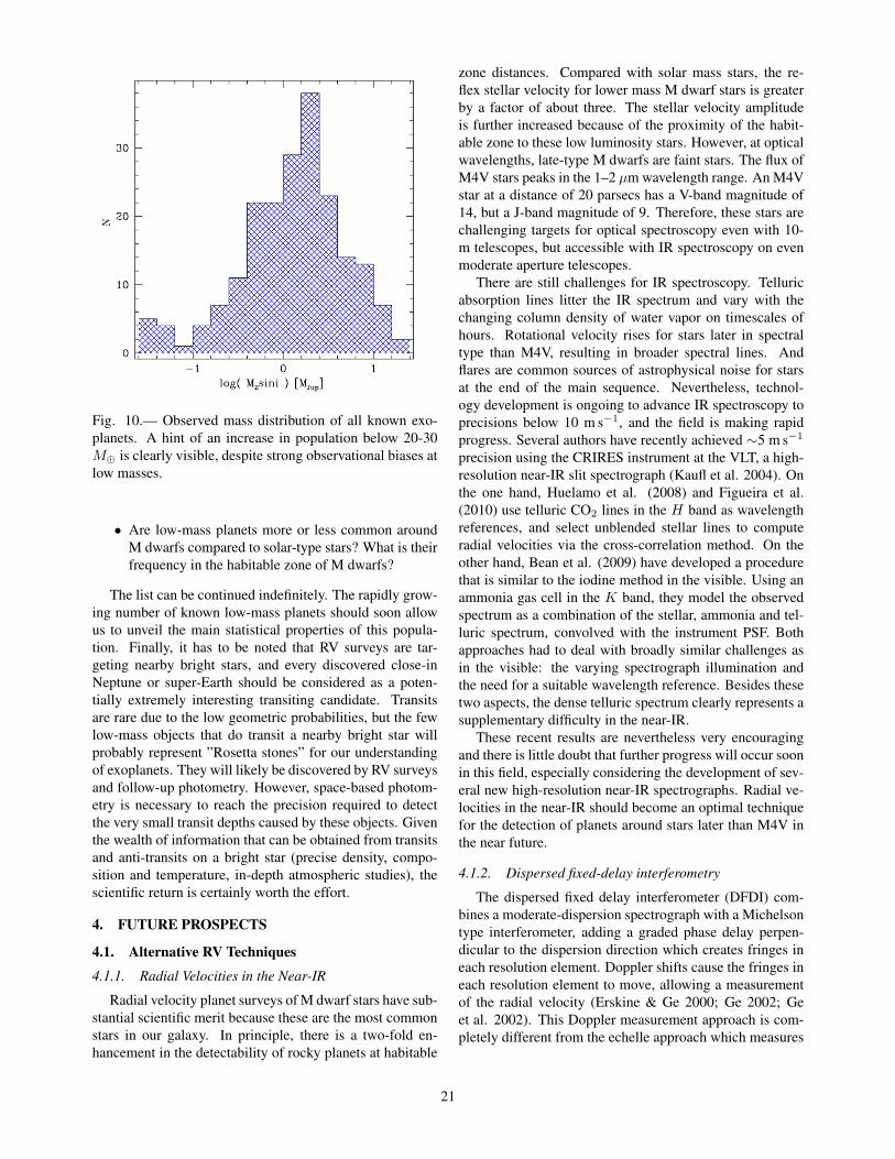
Fig. 10.— Observed mass distribution of all known exo-planets. A hint of an increase in population below 20-30M⊕ is clearly visible, despite strong observational biases atlow masses.

• Are low-mass planets more or less common aroundM dwarfs compared to solar-type stars? What is theirfrequency in the habitable zone of M dwarfs?

The list can be continued indefinitely. The rapidly grow-ing number of known low-mass planets should soon allowus to unveil the main statistical properties of this popula-tion. Finally, it has to be noted that RV surveys are tar-geting nearby bright stars, and every discovered close-inNeptune or super-Earth should be considered as a poten-tially extremely interesting transiting candidate. Transitsare rare due to the low geometric probabilities, but the fewlow-mass objects that do transit a nearby bright star willprobably represent ”Rosetta stones” for our understandingof exoplanets. They will likely be discovered by RV surveysand follow-up photometry. However, space-based photom-etry is necessary to reach the precision required to detectthe very small transit depths caused by these objects. Giventhe wealth of information that can be obtained from transitsand anti-transits on a bright star (precise density, compo-sition and temperature, in-depth atmospheric studies), thescientific return is certainly worth the effort.

4. FUTURE PROSPECTS

4.1. Alternative RV Techniques

4.1.1. Radial Velocities in the Near-IR

Radial velocity planet surveys of M dwarf stars have sub-stantial scientific merit because these are the most commonstars in our galaxy. In principle, there is a two-fold en-hancement in the detectability of rocky planets at habitable

zone distances. Compared with solar mass stars, the re-flex stellar velocity for lower mass M dwarf stars is greaterby a factor of about three. The stellar velocity amplitudeis further increased because of the proximity of the habit-able zone to these low luminosity stars. However, at opticalwavelengths, late-type M dwarfs are faint stars. The flux ofM4V stars peaks in the 1–2 µm wavelength range. An M4Vstar at a distance of 20 parsecs has a V-band magnitude of14, but a J-band magnitude of 9. Therefore, these stars arechallenging targets for optical spectroscopy even with 10-m telescopes, but accessible with IR spectroscopy on evenmoderate aperture telescopes.

There are still challenges for IR spectroscopy. Telluricabsorption lines litter the IR spectrum and vary with thechanging column density of water vapor on timescales ofhours. Rotational velocity rises for stars later in spectraltype than M4V, resulting in broader spectral lines. Andflares are common sources of astrophysical noise for starsat the end of the main sequence. Nevertheless, technol-ogy development is ongoing to advance IR spectroscopy toprecisions below 10 m s−1, and the field is making rapidprogress. Several authors have recently achieved ∼5 m s−1

precision using the CRIRES instrument at the VLT, a high-resolution near-IR slit spectrograph (Kaufl et al. 2004). Onthe one hand, Huelamo et al. (2008) and Figueira et al.(2010) use telluric CO2 lines in the H band as wavelengthreferences, and select unblended stellar lines to computeradial velocities via the cross-correlation method. On theother hand, Bean et al. (2009) have developed a procedurethat is similar to the iodine method in the visible. Using anammonia gas cell in the K band, they model the observedspectrum as a combination of the stellar, ammonia and tel-luric spectrum, convolved with the instrument PSF. Bothapproaches had to deal with broadly similar challenges asin the visible: the varying spectrograph illumination andthe need for a suitable wavelength reference. Besides thesetwo aspects, the dense telluric spectrum clearly represents asupplementary difficulty in the near-IR.

These recent results are nevertheless very encouragingand there is little doubt that further progress will occur soonin this field, especially considering the development of sev-eral new high-resolution near-IR spectrographs. Radial ve-locities in the near-IR should become an optimal techniquefor the detection of planets around stars later than M4V inthe near future.

4.1.2. Dispersed fixed-delay interferometry

The dispersed fixed delay interferometer (DFDI) com-bines a moderate-dispersion spectrograph with a Michelsontype interferometer, adding a graded phase delay perpen-dicular to the dispersion direction which creates fringes ineach resolution element. Doppler shifts cause the fringes ineach resolution element to move, allowing a measurementof the radial velocity (Erskine & Ge 2000; Ge 2002; Geet al. 2002). This Doppler measurement approach is com-pletely different from the echelle approach which measures

21

the absorption line centroid shifts. The Doppler sensitiv-ity of the DFDI approach weakly depends on the spectralresolution compared to the echelle approach (1/2 power ofthe spectral resolution vs. 3/2 power of the spectral resolu-tion in the echelle method, Ge 2002). This allows the useof a medium resolution, but high efficiency spectrometerfor dispersing the fringes to boost the overall detection ef-ficiency, while reducing the instrument size and cost. Also,the DFDI approach takes up a small amount of space on aCCD to cover one dispersion order fringing spectrum witha moderate wavelength coverage (e.g. ∼600 A for the Ex-oplanet Tracker instrument at the Kitt Peak National Ob-servatory 2.1 meter telescope, Ge et al. 2006), which al-lows to either use a multi-object fiber feed so that simulta-neous, high-throughput, high Doppler sensitivity measure-ments of many objects may be made with reasonable de-tector sizes or implement a cross-dispersion mode for largewavelength coverage, high dispersion, high throughput andhigh Doppler sensitivity measurements of a single star (Ge2002; Ge et al. 2007).

To date, one planet has been discovered by the DFDIinstruments, around the star HD 102195 (Ge et al. 2006).Several planet and brown dwarf candidates have been iden-tified from the on-going planet surveys at the Sloan DigitalSky Survey telescope and the KPNO 2.1m telescope andare being followed up with additional observations. A next-generation, multiple-object, DFDI Doppler instrument with60 object capability was commissioned at the SDSS tele-scope at Apache Point Observatory in September 2008 andis being used for conducting the Multi-object APO Radial-Velocity Exoplanet Large-area Survey (MARVELS), whichis one of the four Sloan Digital Sky Survey (SDSS) III sur-vey projects in the period 2008-2014.

4.2. Characterization of Transiting Planets Found bySpace Missions

The space missions CoRoT and Kepler (Baglin et al.2002, Borucki et al. 2003) are both dedicated to the searchof transiting exoplanets by collecting long, high-precisionphotometric time series of thousands of stars. Transit eventshave to pass first through a series of photometric and spec-troscopic tests to exclude alternative scenarios before theycan be confirmed as bona fide transiting planets. High-precision radial velocity measurements are then necessaryto measure the mass of the objects and obtain their meandensity. This follow-up work has already been ongoing withgreat success for CoRoT and several ground-based tran-sit surveys, which are presently discovering a large num-ber of hot Jupiters (e.g. SWASP, HAT). CoRoT and par-ticularly Kepler are expected to also find several hot Nep-tunes and super-Earths, whose mass will have to be mea-sured. This task may be challenging due to the faintnessof the targets and their activity level. However, for quietstars with magnitudes V =11-12, instruments like HARPSand its twin HARPS-North (Latham et al. 2007) will beable to measure the masses of close-in super-Earths down to

∼5 M⊕ with an accuracy (∼10%) that should be sufficientto usefully constrain their mean density and composition.In the near future, the combination of space-based transitsearches and high-precision RV follow-up is thus likely toconsiderably improve our knowledge of the close-in low-mass planet population.

4.3. Pushing down the Limits: towards the Detectionof Earths around Nearby Stars

What are the ultimate limitations of the radial velocitytechnique? To answer this difficult question, it is necessaryto identify which are the dominant sources of systematicerrors. These fall into two general categories: instrumentaland stellar. We first discuss the instrumental aspects, andthen examine stellar noise.

Instrumental limitations are presently fairly well under-stood, and strategies to overcome them are being devel-oped. For HARPS-like instruments, the limiting factorsare mainly the guiding system, the light-scrambling effi-ciency and the wavelength calibration source. For each ofthese issues, it appears that significant progress is possiblecompared to existing facilities like HARPS with relativelymodest technological developments and costs. Tests are on-going on optimized light injection optics and optical fibersto make the spectrograph illumination as homogeneous aspossible. As for wavelength calibration, new solutions suchas the laser frequency comb (see Sect. 2.5) and stabilizedFabry-Perot etalons are being developed and tested.

Two major European instrumental projects are nowbuilding on the HARPS experience with the goal of im-proving the overall stability and precision, but also thephoton collecting power. Indeed, HARPS is not far frombeing photon-limited on the typical stars that are presentlysearched for low-mass planets, so that a larger telescopeaperture is needed if performances are to be significantlyimproved. The first of these projects is ESPRESSO, thesuccessor of HARPS, to be installed on the ESO Very LargeTelescope at Paranal Observatory, Chile (Pepe et al. 2010).ESPRESSO is developed with the goal of achieving an in-strumental precision of 10 cm s−1 on both the short- andlong-term, corresponding to the RV signal induced by theEarth orbiting the Sun. Moreover, ESPRESSO will benefitfrom the large 8.2m aperture of the VLT. It will even bepossible to feed the spectrograph with the four 8.2m tele-scopes simultaneously, which represent the equivalent ofa single 16m aperture. In this mode, the radial velocityprecision will however be somewhat degraded compared tothe single-telescope mode. According to the typical num-bers given in Sect. 2.3, it appears that a SNR of about 700per pixel will be required (at 550 nm) to achieve a photon-limited precision of 10 cm s−1 at R = 140,000. This canbe obtained in about 20 min of exposure time for stars withV =7.5 on a 10-m class telescope. ESPRESSO will thus beable to carry out an extremely precise survey of 100-200nearby bright stars, carefully selected to minimize stellarnoise based on HARPS data. It will find all low-mass plan-

22

ets down to a few Earth masses orbiting within ∼1 AU oftheir parent star, and possibly even 1-M⊕ planets in the hab-itable zones around K and M dwarfs. This survey shouldthus yield a comprehensive picture of telluric planets in thesolar neighborhood.

The other major European project is CODEX, an ultra-stable high-resolution visible spectrograph for the EuropeanExtremely Large Telescope (Pasquini et al. 2008). Theaimed instrumental precision of CODEX is ∼1 cm s−1. Itsmain science objectives all require extremely high Dopplerprecision: measurement of the cosmological redshift driftand the dynamics of the Universe, search for Earth-likeplanets and search for variability in fundamental constants.Although the required performances are quite challenging,there is little doubt that the possibility to address these out-standing scientific issues is well worth the technical effort.The experience gained with HARPS and ESPRESSO is ex-pected to be of great value in this context.

We now turn to the issue of stellar noise in the con-text of the detection of very low-amplitude radial velocitysignals. As described in Sect. 2.4, several physical phe-nomena in stellar photospheres (oscillations, granulation,active regions) may hide planet-induced RV variations atthe m s−1 level and below. To address this problem, stud-ies are ongoing to precisely characterize stellar RV noiseat the relevant timescales (from minutes for oscillations toabout one month for activity). Solar and stellar power den-sity spectra of long, high-precision RV time series can beused to derive the main properties of each noise compo-nent and understand how it varies from star to star. Fromthese results it is possible to find and select the most suitablestars for sub-m s−1 RV monitoring. From what is presentlyknown about stellar noise, it clearly appears that F starsand slightly evolved G and K stars are unsuitable becauseall noise sources become larger in these objects. Betweenunevolved-G and M stars, oscillation and granulation noisebecome smaller, but activity levels tend to be higher in late-K and M stars because of the slower decrease of activitywith age. However, this is partly compensated by the lowermasses of these stars which make RV signals larger for agiven planet mass. Activity-related noise can be minimizedby selecting the stars with the lowest CaII H&K index,and in particular those which do not exhibit activity cycles(or only weak ones). Such objects may be in a Maunder-minimum state, an optimal situation to reach unprecedentedprecision levels on RV measurements. The identification ofthis low-activity population is presently ongoing, makinguse of the thousands of spectra that have been gathered byradial velocity surveys over the past years.

Realistic simulations of the stellar noise, based on ob-served power density spectra, should be made to derive theoptimal observing strategy and compute planet detectionlimits (e.g. Dumusque et al. 2010, in preparation). Prelimi-nary results indicate that a sufficiently dense sampling prop-erly covering the typical timescales of the different noisesources lead to significant improvements in planet detec-tion limits. Moreover, the search for planets in the habit-

able zone may well benefit from the probably low stellarnoise level over timescales of 100-1000 days. As a result,it may well be possible to detect Earth-mass planets in thehabitable zone of G, and particularly K dwarfs. Despite thelow RV amplitudes, solar-like stars should therefore also beconsidered for this kind of searches, together with M dwarfswhich have the obvious advantages of being less massiveand having closer habitable zones. Finally, we note thatthese estimates are not only the result of simulations, butalso of real data: as an example, binning the HARPS RVmeasurements obtained on the star HD 69830 (Lovis et al.2006) over timescales of ∼15 days yields a long-term RVdispersion of only ∼30 cm s−1 (after subtracting the signalof the three known planets). Given all the instrumental er-ror sources and photon noise that contribute to this number,this observational result shows that we are indeed tantaliz-ingly close to being able to detect an Earth-like planet in thehabitable zone of this star.

4.4. Conclusion

In this chapter we have reviewed the history, capabili-ties, achievements and present state-of-the-art of the radialvelocity technique applied to the search for exoplanets. Insummary this technique has, over the past 15 years, openedand developed a new field of astrophysics which has al-ready become one of the most prominent in this discipline,be it in terms of its scientific potential or in terms of thewide-ranging public interest associated to it. After the ini-tial gas giant era, the RV technique has now fully enteredthe domain of low-mass planets. Given the achieved detec-tion limits, present and near-future RV surveys of nearbybright stars will unveil the statistical properties of the low-mass planet population within ∼1 AU. We will then have aglobal picture of exoplanets, from massive gas giants to tel-luric bodies, and this will allow us to make decisive steps inour understanding of planet formation and migration. Thisis all the more true in cases where the RV technique can becoupled to the transit technique. As other detection tech-niques appear and are developed, radial velocities will re-main a fundamental tool to obtain dynamical masses andcharacterize systems. As an important by-product, the ob-tained high-resolution spectra can be used to characterizethe host star. Detecting exoplanets is and will remain anobservational challenge requiring significant efforts in in-strumental developments. While all possible approachesshould certainly be explored, the cost-effectiveness of theRV technique should be particularly emphasized, and thusthe development of improved RV facilities should certainlybe continued in the future.

Acknowledgments.

23

REFERENCES

Alibert, Y., Baraffe, I., Benz, W., et al. (2006) Formation andstructure of the three Neptune-mass planets system around HD69830. Astron. Astrophys., 455, L25-L28.

Baglin, A., Auvergne, M., Barge, P., et al. (2002) COROT: as-teroseismology and planet finding. In Proceedings of the FirstEddington Workshop on Stellar Structure and Habitable PlanetFinding, ESA Spec. Publ., 485 (B. Battrick et al., eds.), 17-24.

Bakos, G. A., Torres, G., Pal, A., et al. (2010) HAT-P-11b:A Super-Neptune Planet Transiting a Bright K Star in theKepler Field. Accepted for publication in Astrophys. J.,arXiv:0901.0282.

Baliunas, S. L., Donahue, R. A., Soon, W. H., et al. (1995) Chro-mospheric variations in main-sequence stars. Astrophys. J.,438, 269-287.

Baranne, A., Queloz, D., Mayor, M., et al. (1996) ELODIE: Aspectrograph for accurate radial velocity measurements.. As-tron. Astrophys. Supp. Ser., 119, 373-390.

Bean, J. L., Seifahrt, A., Hartman, H., et al. (2009) The CRIRESSearch for Planets Around the Lowest-Mass Stars. I. High-Precision Near-Infrared Radial Velocities with an AmmoniaGas Cell. Astrophys. J., in press, arXiv:0911.3148.

Beichman, C. A., Bryden, G., Gautier, T. N., et al. (2005) AnExcess Due to Small Grains around the Nearby K0 V StarHD 69830: Asteroid or Cometary Debris? Astrophys. J., 626,1061-1069.

Blake, C. (2008) UNKNOWN REFERENCEBonfils, X., Delfosse, X., Udry, S., et al. (2006) Any hot-Jupiter

around M dwarfs? In Tenth Anniversary of 51 Peg-b: Status ofand prospects for hot Jupiter studies (L. Arnold et al., eds.),111-118.

Bonfils, X., Forveille, T., Delfosse, X., et al. (2005) The HARPSsearch for southern extra-solar planets. VI. A Neptune-massplanet around the nearby M dwarf Gl 581. Astron. Astrophys.,443, L15-L18.

Bonfils, X., Mayor, M., Delfosse, X., et al. (2007) The HARPSsearch for southern extra-solar planets. X. A m sin i = 11 M⊕planet around the nearby spotted M dwarf GJ 674. Astron. As-trophys., 474, 293-299.

Borucki, W. J., Koch, D. G., Lissauer, J. J., et al. (2003) The Ke-pler mission: a wide-field-of-view photometer designed to de-termine the frequency of Earth-size planets around solar-likestars. In Future EUV/UV and Visible Space Astrophysics Mis-sions and Instrumentation, Proc. Soc. Photo-Opt. Instrum.Eng., 4854 (J.C. Blades et al., eds.), 129-140.

Bouchy, F., and Carrier, F. (2001) P-mode observations on α CenA. Astron. Astrophys., 374, L5-L8.

Bouchy, F., Pepe, F., and Queloz, D. (2001) Fundamental pho-ton noise limit to radial velocity measurements. Astron. Astro-phys., 374, 733-739.

Bouchy, F., Mayor, M., Lovis, C., et al. (2009) The HARPSsearch for southern extra-solar planets. XVII. Super-Earth andNeptune-mass planets in multiple planet systems HD 47 186and HD 181 433. Astron. Astrophys., 496, 527-531.

Bouchy, F., and The Sophie Team (2006) SOPHIE: the successorof the spectrograph ELODIE for extrasolar planet search andcharacterization. In Tenth Anniversary of 51 Peg-b: Status ofand prospects for hot Jupiter studies (L. Arnold et al., eds.),319-325.

Braje, D. A., Kirchner, M. S., Osterman, S., et al. (2008) As-

tronomical spectrograph calibration with broad-spectrum fre-quency combs. Eur. Phys. J. D, 48, 57-66.

Butler, R. P., and Marcy, G. W. (1996) A Planet Orbiting 47 UrsaeMajoris. Astrophys. J. Lett., 464, L153-L156.

Butler, R. P., Marcy, G. W., Williams, E., et al. (1996) AttainingDoppler Precision of 3 m s−1. Publ. Astron. Soc. Pac., 108,500-509.

Butler, R. P., Marcy, G. W., Williams, E., et al. (1997) ThreeNew ”51 Pegasi–Type” Planets. Astrophys. J. Lett., 474, L115-L118.

Butler, R. P., Vogt, S. S., Marcy, G. W., et al. (2004) A Neptune-Mass Planet Orbiting the Nearby M Dwarf GJ 436. Astrophys.J., 617, 580-588.

Campbell, B. and Walker, G. A. H (1979) Precision radial veloci-ties with an absorption cell. Publ. Astron. Soc. Pac., 91, 540-545.

Campbell, B., Walker, G. A. H., and Yang, S. (1988) A search forsubstellar companions to solar-type stars. Astrophys. J., 331,902-921.

Charbonneau, D., Brown, T. M., Latham, D. W., et al. (2000) De-tection of Planetary Transits Across a Sun-like Star. Astrophys.J. Lett., 529, L45-L48.

Christensen-Dalsgaard, J. (2004) Physics of solar-like oscillations.In Sol. Phys., 220, Issue 2, 137-168.

Connes, P. (1985) Absolute astronomical accelerometry. Astro-phys. Space Sci., 110, 211-255.

Delfosse, X., Forveille, T., Mayor, M., et al. (1998) The closestextrasolar planet. A giant planet around the M4 dwarf GL 876.Astron. Astrophys., 338, L67-L70.

Desort, M., Lagrange, A.-M., Galland, F., et al. (2007) Searchfor exoplanets with the radial-velocity technique: quantitativediagnostics of stellar activity. Astron. Astrophys., 473, 983-993.

Dollinger, M. P., Hatzes, A. P., Pasquini, L., et al. (2007) Discov-ery of a planet around the K giant star 4 Ursae Majoris. Astron.Astrophys., 472, 649-652.

Dravins, D. (1990) Stellar granulation. VI - Four-component mod-els and non-solar-type stars. Astron. Astrophys., 228, 218-230.

Einstein, A. (1905) Zur Elektrodynamik bewegter Korper. Ann.Phys., 322, 891-921.

Endl, M., Cochran, W. D., Kurster, M., et al. (2006) Exploringthe Frequency of Close-in Jovian Planets around M Dwarfs.Astrophys. J., 649, 436-443.

Erskine, D. J., and Ge, J. (2000) A Novel Interferometer Spec-trometer for Sensitive Stellar Radial Velocimetry. In Imagingthe Universe in Three Dimensions, Publ. Astron. Soc. Pac.Conf. Ser., 195 (W. van Breugel and J. Bland-Hawthorn, eds.),501-507

Fienga, A., Manche, H., Laskar, J., et al. (2008) INPOP06: a newnumerical planetary ephemeris. Astron. Astrophys., 477, 315-327.

Figueira, P., Pepe, F., Melo, C. H. F., et al. (2009) Radial Velocitieswith CRIRES: Pushing precision down to 5-10 m/s. Astron.Astrophys., in press, arXiv:0912.2643.

Fischer, D. A., Marcy, G. W., Butler, R. P., et al. (2008) Five Plan-ets Orbiting 55 Cancri. Astrophys. J., 675, 790-801.

Fischer, D. A., Vogt, S. S., Marcy, G. W., et al. (2007) FiveIntermediate-Period Planets from the N2K Sample. Astrophys.J., 669, 1336-1344.

Forveille, T., Bonfils, X., Delfosse, X., et al. (2009) The HARPSsearch for southern extra-solar planets. XIV. Gl 176b, a super-Earth rather than a Neptune, and at a different period. Astron.

24

Astrophys., 493, 645-650.Frink, S., Mitchell, D. S., Quirrenbach, A., et al. (2002) Discov-

ery of a Substellar Companion to the K2 III Giant ι Draconis.Astrophys. J., 576, 478-484.

Galland, F., Lagrange, A.-M., Udry, S., et al. (2005) Extrasolarplanets and brown dwarfs around A-F type stars. II. A planetfound with ELODIE around the F6V star HD 33564. Astron.Astrophys., 444, L21-L24.

Galland, F., Lagrange, A.-M., Udry, S., et al. (2006) Extrasolarplanets and brown dwarfs around A-F type stars. IV. A candi-date brown dwarf around the A9V pulsating star HD 180777.Astron. Astrophys., 452, 709-714.

Ge, J. (2002) Fixed Delay Interferometry for Doppler ExtrasolarPlanet Detection. Astrophys. J. Lett., 571, L165-L168.

Ge, J., Erskine, D. J., and Rushford, M. (2002) An Externally Dis-persed Interferometer for Sensitive Doppler Extrasolar PlanetSearches. Publ. Astron. Soc. Pac., 114, 1016-1028.

Ge, J., van Eyken, J., Mahadevan, S., et al. (2006) The FirstExtrasolar Planet Discovered with a New-Generation High-Throughput Doppler Instrument. Astrophys. J., 648, 683-695.

Ge, J., van Eyken, J. C., Mahadevan, S., et al. (2007) An All SkyExtrasolar Planet Survey with New Generation Multiple ObjectDoppler Instruments at Sloan Telescope. Rev. Mex. AstronAstrophys. Conf. Ser., 29, 30-36.

Gillon, M., Pont, F., Demory, B.-O., et al. (2007) Detection oftransits of the nearby hot Neptune GJ 436 b. Astron. Astro-phys., 472, L13-L16.

Griffin, R. and Griffin, R. (1973) Accurate wavelengths of stel-lar and telluric absorption lines near lambda 7000 Angstroms.Mon. Not. Roy. Astr. Soc., 162, 255-260.

Hatzes, A. P., and Cochran, W. D. (1993) Long-period radial ve-locity variations in three K giants. Astrophys. J., 413, 339-348.

Hekker, S., Snellen, I. A. G., Aerts, C., et al. (2008) Precise ra-dial velocities of giant stars. IV. A correlation between surfacegravity and radial velocity variation and a statistical investiga-tion of companion properties. Astron. Astrophys., 480, 215-222.

Henry, G. W., Marcy, G. W., Butler, R. P., et al. (2000) A Transit-ing “51 Peg-like” Planet. Astrophys. J. Lett., 529, L41-L44.

Howard, A. W., Johnson, J. A., Marcy, G. W., et al. (2009) TheNASA-UC Eta-Earth Program. I. A Super-Earth Orbiting HD7924. Astrophys. J., 696, 75-83.

Huelamo, N., Figueira, P., Bonfils, X., et al. (2008) TW Hydrae:evidence of stellar spots instead of a Hot Jupiter. Astron. As-trophys., 489, L9-L13.

Ida, S., and Lin, D. N. C. (2005) Toward a Deterministic Modelof Planetary Formation. III. Mass Distribution of Short-PeriodPlanets around Stars of Various Masses. Astrophys. J., 626,1045-1060.

Ida, S., and Lin, D. N. C. (2008) Toward a Deterministic Model ofPlanetary Formation. V. Accumulation Near the Ice Line andSuper-Earths. Astrophys. J., 685, 584-595.

Johnson, J. A., Butler, R. P., Marcy, G. W., et al. (2007a) A NewPlanet around an M Dwarf: Revealing a Correlation betweenExoplanets and Stellar Mass. Astrophys. J., 670, 833-840.

Johnson, J. A., Fischer, D. A., Marcy, G. W., et al. (2007b) RetiredA Stars and Their Companions: Exoplanets Orbiting ThreeIntermediate-Mass Subgiants. Astrophys. J., 665, 785-793.

Kaeufl, H.-U., Ballester, P., Biereichel, P., et al. (2004) CRIRES:a high-resolution infrared spectrograph for ESO’s VLT. InGround-based Instrumentation for Astronomy, Proc. Soc.Photo-Opt. Instrum. Eng., 5492 (A.F.M. Moorwood and I.

Masanori, eds.), 1218-1227.Kennedy, G. M., and Kenyon, S. J. (2008) Planet Formation

around Stars of Various Masses: The Snow Line and the Fre-quency of Giant Planets. Astrophys. J., 673, 502-512.

Kjeldsen, H., Bedding, T. R., Butler, R. P., et al. (2005) Solar-likeOscillations in α Centauri B. Astrophys. J., 635, 1281-1290.

Kurster, M., Hatzes, A. P., Cochran, W. D., et al. (1999) Preciseradial velocities of Proxima Centauri. Strong constraints on asubstellar companion. Astron. Astrophys., 344, L5-L8.

Latham, D. W. (2007) Hot Earths: Prospects For Detection ByKepler And Characterization with HARPS-NEF. Bull. Am. As-tron. Soc., 38, 234.

Latham, D. W., Stefanik, R. P., Mazeh, T., et al. (1989) The unseencompanion of HD114762 - A probable brown dwarf. Nature,339, 38-40.

Laughlin, G., Bodenheimer, P., and Adams, F. C. (2004) The CoreAccretion Model Predicts Few Jovian-Mass Planets OrbitingRed Dwarfs. Astrophys. J. Lett., 612, L73-L76.

Li, C.-H., Benedick, A. J., Fendel, P., et al. (2008) A laser fre-quency comb that enables radial velocity measurements with aprecision of 1cm s−1. Nature, 452, 610-612.

Lindegren, L., and Dravins, D. (2003) The fundamental definitionof “radial velocity”. Astron. Astrophys., 401, 1185-1201.

Lisse, C. M., Beichman, C. A., Bryden, G., et al. (2007) On theNature of the Dust in the Debris Disk around HD 69830. As-trophys. J., 658, 584-592.

Lovis, C., and Pepe, F. (2007) A new list of thorium and argonspectral lines in the visible. Astron. Astrophys., 468, 1115-1121.

Lovis, C., and Mayor, M. (2007) Planets around evolved intermediate-mass stars. I. Two substellar companions in the open clustersNGC 2423 and NGC 4349. Astron. Astrophys., 472, 657-664.

Lovis, C., Mayor, M., Bouchy, F., et al. (2009) Towards the char-acterization of the hot Neptune/super-Earth population aroundnearby bright stars. In Transiting Planets, Proc. Int. Astron.Union, 253, 502-505.

Lovis, C., Mayor, M., Pepe, F., et al. (2006) An extrasolar plan-etary system with three Neptune-mass planets. Nature, 441,305-309.

Marcy, G. W., and Butler, R. P. (1995) The Planet around 51 Pe-gasi. Bull. Am. Astron. Soc., 27, 1379.

Marcy, G. W., and Butler, R. P. (1996) A Planetary Companion to70 Virginis. Astrophys. J. Lett., 464, L147-L151.

Marcy, G. W., Butler, R. P., Fischer, D., et al. (2001) A Pair ofResonant Planets Orbiting GJ 876. Astrophys. J., 556, 296-301.

Marcy, G. W., Butler, R. P., Vogt, S. S., et al. (1998) A PlanetaryCompanion to a Nearby M4 Dwarf, Gliese 876. Astrophys. J.Lett., 505, L147-L149.

Mayor, M., Bonfils, X., Forveille, T., et al. (2009b) The HARPSsearch for southern extra-solar planets. XVIII. An Earth-massplanet in the GJ 581 planetary system. Astron. Astrophys., 507,487-494.

Mayor, M., Pepe, F., Queloz, D., et al. (2003) Setting New Stan-dards with HARPS. The Messenger, 114, 20-24.

Mayor, M., and Queloz, D. (1995) A Jupiter-mass companion to asolar-type star. Nature, 378, 355-359.

Mayor, M., Udry, S., Lovis, C., et al. (2009a) The HARPS searchfor southern extra-solar planets. XIII. A planetary system with3 super-Earths (4.2, 6.9, and 9.2 M⊕). Astron. Astrophys., 493,639-644.

McArthur, B. E., Endl, M., Cochran, W. D., et al. (2004) Detection

25

of a Neptune-Mass Planet in the ρ1 Cancri System Using theHobby-Eberly Telescope. Astrophys. J. Lett., 614, L81-L84.

Melo, C., Santos, N. C., Gieren, W., et al. (2007) A new Neptune-mass planet orbiting HD 219828. Astron. Astrophys., 467, 721-727.

Mordasini, C., Alibert, Y., Benz, W., et al. (2009) Extrasolar planetpopulation synthesis. I. Method, formation tracks, and mass-distance distribution. Astron. Astrophys., 501, 1139-1160.

Murphy, M. T., Udem, T., Holzwarth, R., et al. (2007) High-precision wavelength calibration of astronomical spectro-graphs with laser frequency combs. Mon. Not. Roy. Astr. Soc.,380, 839-847.

Naef, D., Latham, D. W., Mayor, M., et al. (2001) HD 80606 b,a planet on an extremely elongated orbit. Astron. Astrophys.,375, L27-L30.

Niedzielski, A., Konacki, M., Wolszczan, A., et al. (2007) APlanetary-Mass Companion to the K0 Giant HD 17092. As-trophys. J., 669, 1354-1358.

O’Toole, S., Tinney, C. G., Butler, R. P., et al. (2009) A Neptune-mass Planet Orbiting the Nearby G Dwarf HD 16417. Astro-phys. J., 697, 1263-1268.

Palle, P. L., Jimenez, A., Perez Hernandez, F., et al. (1995) Ameasurement of the background solar velocity spectrum. As-trophys. J., 441, 952-959.

Pasquini, L., Avila, G., Dekker, H., et al. (2008) CODEX: thehigh-resolution visual spectrograph for the E-ELT. In Ground-based and Airborne Instrumentation for Astronomy II, Proc.Soc. Photo-Opt. Instrum. Eng., 7014 (I.S. McLean and M.M.Casali, eds.), 70141I.

Pasquini, L., Dollinger, M. P., Weiss, A., et al. (2007) Evolvedstars suggest an external origin of the enhanced metallicity inplanet-hosting stars. Astron. Astrophys., 473, 979-982.

Pepe, F., Correia, A. C. M., Mayor, M., et al. (2007) The HARPSsearch for southern extra-solar planets. VIII. µ Arae, a systemwith four planets. Astron. Astrophys., 462, 769-776.

Pepe, F., Mayor, M., Galland, F., et al. (2002) The CORALIEsurvey for southern extra-solar planets VII. Two short-periodSaturnian companions to HD 108147 and HD 168746. Astron.Astrophys., 388, 632-638.

Pepe, F., Cristiani, S., Rebolo Lopez, R., et al. (2010) ESPRESSO- Exploring science frontiers with extreme-precision spec-troscopy. In Ground-based and Airborne Instrumentation forAstronomy III, Proc. Soc. Photo-Opt. Instrum. Eng., in press(I.S. McLean et al., eds.).

Queloz, D., Henry, G. W., Sivan, J. P., et al. (2001) No planet forHD 166435. Astron. Astrophys., 379, 279-287.

Queloz, D., Mayor, M., Weber, L., et al. (2000) The CORALIEsurvey for southern extra-solar planets. I. A planet orbiting thestar Gliese 86. Astron. Astrophys., 354, 99-102.

Rickman, H. (2001) Transactions of the International Astronomi-cal Union Proceedings of the Twenty-Fourth General Assem-bly.. In Transactions of the International Astronomical Union,Astron. Soc. Pac. Ser. B, 24 (H. Rickman, ed.).

Rivera, E. J., Lissauer, J. J., Butler, R. P., et al. (2005) A 7.5 M⊕Planet Orbiting the Nearby Star, GJ 876. Astrophys. J., 634,625-640.

Saar, S. H., and Donahue, R. A. (1997) Activity-related RadialVelocity Variation in Cool Stars. Astrophys. J., 485, 319-327.

Saar, S. H., and Fischer, D. (2000) Correcting Radial Velocities forLong-Term Magnetic Activity Variations. Astrophys. J. Lett.,534, L105-L108.

Santos, N. C., Bouchy, F., Mayor, M., et al. (2004) The HARPS

survey for southern extra-solar planets. II. A 14 Earth-massesexoplanet around µ Arae. Astron. Astrophys., 426, L19-L23.

Santos, N. C., Mayor, M., Naef, D., et al. (2000) The CORALIEsurvey for Southern extra-solar planets. IV. Intrinsic stellarlimitations to planet searches with radial-velocity techniques.Astron. Astrophys., 361, 265-272.

Sato, B., Ando, H., Kambe, E., et al. (2003) A Planetary Compan-ion to the G-Type Giant Star HD 104985. Astrophys. J. Lett.,597, L157-L160.

Sato, B., Fischer, D. A., Henry, G. W., et al. (2005) The N2KConsortium. II. A Transiting Hot Saturn around HD 149026with a Large Dense Core. Astrophys. J., 633, 465-473.

Selsis, F., Kasting, J. F., Levrard, B., et al. (2007) Habitable plan-ets around the star Gliese 581? Astron. Astrophys., 476, 1373-1387.

Setiawan, J., Hatzes, A. P., von der Luhe, O., et al. (2003) Ev-idence of a sub-stellar companion around HD 47536. Astron.Astrophys., 398, L19-L23.

Standish, E. M., Jr. (1990) The observational basis for JPL’s DE200, the planetary ephemerides of the Astronomical Almanac.Astron. Astrophys., 233, 252-271.

Steinmetz, T., Wilken, T., Araujo-Hauck, C., et al. (2008) LaserFrequency Combs for Astronomical Observations. Science,321, 1335-1337.

Struve, O. (1952) Proposal for a project of high-precision stellarradial velocity work. The Observatory, 72, 199-200.

Udry, S., Bonfils, X., Delfosse, X., et al. (2007) The HARPSsearch for southern extra-solar planets. XI. Super-Earths (5 and8 M⊕) in a 3-planet system. Astron. Astrophys., 469, L43-L47.

Udry, S., Mayor, M., Benz, W., et al. (2006) The HARPS searchfor southern extra-solar planets. V. A 14 Earth-masses planetorbiting HD 4308. Astron. Astrophys., 447, 361-367.

Udry, S., and Santos, N. C. (2007) Statistical Properties of Exo-planets. Ann. Rev. Astron. Astrophys., 45, 397-439.

Valenti, J. A., Butler, R. P., and Marcy, G. W. (1995) Determin-ing Spectrometer Instrumental Profiles Using FTS ReferenceSpectra. Publ. Astron. Soc. Pac., 107, 966-976.

Vogt, S. S., Butler, R. P., Marcy, G. W., et al. (2005) Five NewMulticomponent Planetary Systems. Astrophys. J., 632, 638-658.

Walker, G. A. H., Walker, A. R., Irwin, A. W., et al. (1995) Asearch for Jupiter-mass companions to nearby stars.. Icarus,116, 359-375.

Wilson, O. C. (1978) Chromospheric variations in main-sequencestars. Astrophys. J., 226, 379-396.

Wilson, R. E. (1953) General Catalogue of Stellar Radial Veloci-ties. Carnegie Inst. Washington D.C. Publ., 601, 1953.

Wolszczan, A., and Frail, D. A. (1992) A planetary system aroundthe millisecond pulsar PSR1257 + 12. Nature, 355, 145-147.

Wright, J. T. (2005) Radial Velocity Jitter in Stars from the Cali-fornia and Carnegie Planet Search at Keck Observatory. Publ.Astron. Soc. Pac., 117, 657-664.

26