Predicting coastal eutrophication in the Baltic: a limnological approach

Predicting coastal eutrophication in the Baltic:a limnological approach

Jessica J. Meeuwig, Pirkko Kauppila, and Heikki Pitkänen

Abstract: Coastal eutrophication is a key environmental concern in Finland. A highly indented, well-settled coastlinewith a myriad of small estuaries means that eutrophication occurs at numerous localities. There is a clear need for gen-eral models that predict eutrophication across estuaries. Lake eutrophication has been successfully predicted using acombination of chlorophylla (Chl) – total phosphorus (TP) regression models and TP mass-balance models. We ap-plied this limnological approach to 19 Finnish estuaries. The Chl–TP regression was highly significant, accounting for67% of the variation in Chl. When combined with a TP mass-balance equation, log observed and predicted Chl dif-fered by 28% on average. Accuracy was improved by dividing the estuaries into those dominated by non-point-source(NPS) loading (n = 11) and those dominated by point-source (PS) loading (n = 7). A land-use regression model basedon percentage of the catchment forested and estuarine mean depth then best predicted Chl in the NPS-dominated estu-aries. The mass-balance approach remained the most accurate model for the PS estuaries. The land-use model andmass-balance approach are complementary tools in that their use maximizes accuracy for both NPS- and PS-dominatedestuaries. This high level of accuracy demonstrates the relevance of limnological approaches to Finnish estuaries.

Résumé: L’eutrophisation du littoral est un problème environnemental grave en Finlande. Étant donné que la ligne decôte est extrêmement découpée et fortement colonisée, et compte une myriade de petits estuaires, l’eutrophisation semanifeste à de nombreux endroits. Il est clairement nécessaire d’établir les modèles généraux permettant de prédirel’eutrophisation d’un estuaire à l’autre. Dans le cas des lacs, on a réussi à prédire l’eutrophisation grâce à une combi-naison de modèles de régression chlorophylle (Chl) / phosphore total (PT) et de modèles du bilan massique du PT.Nous avons appliqué cette approche limnologique à 19 estuaires finnois. La régression Chl:PT était fortement significa-tive, puisqu’elle rendait compte de 67 % de la variation de Chl. Si on y combinait une équation du bilan massique duPT, la différence des logarithmes des valeurs observées et prédites de Chl était de 28 % en moyenne. Nous avons amé-lioré la précision en séparant les estuaires entre ceux qui étaient dominés par une charge de pollution diffuse (PD) (n =11) et ceux qui étaient dominés par une charge de pollution ponctuelle (PP) (n = 7). Un modèle de régression del’utilisation des terres basé sur le pourcentage boisé du bassin et la profondeur moyenne de l’estuaire donnait alors lesmeilleures prédictions pour Chl dans les estuaires dominés par la pollution diffuse. L’approche du bilan massique de-meurait le modèle le plus exact pour les estuaires à pollution ponctuelle. Le modèle de l’tilisation des terres etl’approche du bilan massique sont des outils complémentaires du fait que leur utilisation maximise la précision pourles deux types d’estuaires. Ce haut niveau de précision montre la pertinence des approches limnologiques pour les es-tuaires finnois.

[Traduit par la Rédaction] Meeuwig et al. 855

Introduction

Coastal eutrophication has been identified as a globalproblem from temperate estuaries (Rosenberg 1990) to tropi-cal waters (Lapointe and Clark 1992). It manifests as an in-crease in phytoplankton and macroalgal biomass, increasedincidences of toxic and noxious blooms, hypoxia and an-oxia, and fish and benthos kills (Fisher et al. 1995). The Bal-tic Sea is perhaps one of the first coastal systems in whicheutrophication was identified (Rosenberg 1990), and it con-

tinues to be a key environmental concern (HELCOM 1997).Finland’s coastal waters are particularly sensitive to coastaleutrophication: they are generally shallow, and water ex-change with the open Baltic is restricted due to the complexcoastal morphometry (Bonsdorff et al. 1997). Nutrient loadsare derived from agriculture (Rekolainen et al. 1995), mu-nicipal and industrial wastes (Pitkänen 1994), and fish farms(Bonsdorff et al. 1997). Finland has a long and highly in-dented coastline (39 000 km; Pitkänen 1994) that includesapproximately 50 river-fed estuaries as well as numerousembayments. Human settlement, while concentrated in thesouth and southwest, occurs along the entire coastline. Sucha coastline and settlement pattern mean that eutrophicationis not a localized problem; rather, it occurs in a number ofestuaries from the eastern Gulf of Finland to the northeastBothnian Bay.

The Baltic Sea has received much attention in terms ofmodeling eutrophication (Wulff et al. 1990). However, muchof Finland’s coastline comprises a myriad of small estuariesfor which eutrophication models have not been developed.

Can. J. Fish. Aquat. Sci.57: 844–855 (2000) © 2000 NRC Canada

844

Received September 15, 1998. Accepted December 23, 1999.J14785

J.J. Meeuwig.1 Department of Biology, McGill University,1205 ave. Dr. Penfield, Montreal, QC H3A 1B1, Canada.P. Kauppila and H. Pitkänen. Finnish Environment Institute,P.O. Box 140, FIN-00251 Helsinki, Finland.

1Author to whom all correspondence should be addressed.e-mail: [email protected]

J:\cjfas\cjfas57\cjfas-04\F00-013.vpTuesday, April 04, 2000 1:55:50 PM

Color profile: DisabledComposite Default screen

Given constraints on human and financial resources, it isalso unlikely that site-specific models will be developed forthe majority of small estuaries. Thus, there is a need to de-velop general models that predict eutrophication for a vari-ety of systems. To be relevant to environmental managers,these models must (i) be accurate, (ii ) link the eutrophicationresponse with variables that can be managed, and (iii ) quan-tify the error associated with predictions so that decision riskcan be evaluated.

Such models have been developed to address lake eutro-phication. OECD (1982) used a mass-balance approach toestimate total phosphorus (TP) concentrations in lakes as afunction of TP loading (estimated from land-use activities),water residence time, and P sedimentation. The TP estimatefrom a mass-balance equation is then used in a regressionmodel (e.g., Dillon and Rigler 1974; OECD 1982) that pre-dicts response variables of concern, typically phytoplanktonbiomass (as chlorophylla (Chl)). This approach has formedthe basis of successful lake eutrophication management bothin Europe and North America (OECD 1982). Meeuwig andPeters (1996) demonstrated that regression models based onland use also accurately predict Chl and are an alternative tothe P-based mass-balance approach.

In Finland, riverborne nutrients have been identified as themajor source of excess nutrients both within estuaries and inthe open coastal waters (e.g., Pitkänen 1994). These nutri-ents are derived primarily from agricultural activities and toa lesser extent from point-source waste waters (Rekolainenet al. 1995). To date, strong relationships have been devel-oped to predict total nitrogen (TN) and TP loads as a func-tion of land use (r 2 = 0.80 and 0.73, respectively; Pitkänen1994). However, no analogous empirical models have yetbeen developed to predict phytoplankton biomass in Finnishestuaries as a function of either ambient nutrient concentra-tions, nutrient loads, or land use. Nor has the mass-balanceapproach, so successful in lakes, been applied to these sys-tems despite the fact that these Baltic estuaries are thoughtto be P limited (Pitkänen and Tamminen 1994). We havecompiled a data set for 19 estuaries and their watersheds totest the hypothesis that the mass-balance approach accu-rately predicts Chl in Finnish estuaries. To test this hypothe-sis, we must demonstrate that (i) total nutrients (TN and TP)accurately estimate estuarine Chl, (ii ) mass-balance modelsaccurately estimate TP, and (iii ) TP estimated from mass-balances accurately estimates estuarine Chl. We also testedthe hypothesis that land use, which integrates a number offactors affecting phytoplankton biomass, better estimatesChl than TP or the mass-balance approach.

Materials and methods

Description of data setData were compiled for 19 estuaries located on the Baltic coast

of Finland from the northeast Bothnian Bay to the eastern Gulf ofFinland, near Russia (Fig. 1). Each estuary is hence referred to bythe name of the river with which it is associated (Table 1). Thedata set includes information on: phytoplankton biomass (as Chl),water chemistry, coastal morphometry, land use, and total nutrientloads (Table 1). Chl and water chemistry data are from monitoringsurveys between 1989 and 1993 conducted by the Regional Envi-ronmental Centers of Finland and coordinated by the Finnish Envi-ronment Institute. TP, TN, and conductivity were measured along

vertical profiles, while Chl was measured from integrated watersamples from the surface to 5 m. Chl, TP, and TN were analyzedfrom unfiltered samples using Finnish standard methods (Pitkänen1994). Conductivity (C, millisiemens per metre) was also mea-sured and used to estimate salinity (S, parts per thousand) (Na-tional Board of Waters 1981):

(1) S = (C – 60.91) × 163–1.

There are altogether approximately 500 sampling stations in thecoastal waters monitoring program. Of these 500 stations, we in-cluded 176 stations that were located “within” the estuaries.Estuarine boundaries are typically difficult to define. We used ageographical approach, drawing the outer limit of the estuaryacross the narrowest part of the outermost headlands. Growing sea-son averages were calculated for Chl, TP, TN, and salinity using allmeasurements taken at depths less than 5 m between June and Au-gust.

Most estuaries included in the study were well sampled (Ta-ble 2). Of the 19 estuaries, 12 included data for five years. Spa-tially, there was an average of 4.2 stations per estuary with fiveestuaries represented by a single station. These five estuaries weregenerally the smaller systems (mean surface area = 23 km2 versus48 km2 for all estuaries). Although represented by a single station,three of these five estuaries were sampled three to six times duringthe growing season. Temporally, the sampling effort in a given areavaries depending on the source and amounts of loading and localhydrographical conditions. The sampling frequency ranges in gen-eral from two to 20 times per year, being most typically from fourto six times per year. In our data set, the mean number of samplesper growing season was 3.4 and the mode was 2.

Phytoplankton biomass and nutrients are strongly affected byvariation in hydrology (Schaub and Gieskes 1991), which variesannually. We incorporated this interannual variability by calculat-ing mean valuesXmean for each estuary as

(2) X nm

m i

s

s i

mmean=ms

=

=

=

=

ååæ

è

ççç

ö

ø

÷÷÷

-é

ë

êêê

ù

û

úúú

ì

íïï

11

1

îïï

ü

ýïï

þïï

- -

=

=

å n ns yy

y i

1 1

1

y

whereX is the value for the variable of interest in a given year (y)at a given station (s) in a given month (m) andn indicates the num-ber of years (y), stations (s), or months (m). This averaging ap-proach gives equal weight to each year even if the year isrepresented by a single station. By emphasizing years, we were alsoable to better match the water chemistry data to the hydrologic flowand nutrient loading data that were calculated on a yearly basis.

Estuarine surface area and mean depth were calculated from 1 :50 000 bathymetric charts (Finnish Institute of Navigation 1996–1998). Surface area was measured by planimetry. Mean depth wasestimated using a grid technique whereby the depth under eachsquare of the grid covering the estuary was recorded and the aver-age of these values taken. The mean depths estimated using thisapproach may overestimate the true mean depths, as the availablebathymetric charts did not indicate depths for the shallower fring-ing areas at the mouths of the rivers. These areas were, however,generally small relative to the total surface area.

Water residence time (years) was calculated using two differentapproaches: (i) Bowden’s (1980) saltwater fraction method and(ii ) freshwater replacement (Vollenweider 1975). Mean salinity forBowden’s (1980) method was calculated for the entire estuary aswere the Chl and nutrient mean values. Freshwater inflow was cal-culated for each year from 1989 to 1993. Mean values for each es-tuary were then calculated by averaging values for those years forwhich Chl and nutrient data were available.

Catchment size and land-use data from the early 1990s were ob-tained from the databases of the Finnish Environment Institute fol-

© 2000 NRC Canada

Meeuwig et al. 845



lowing Pitkänen (1994). Human population density was estimatedusing Arc Info by overlaying municipal and watershed boundaries(Finnish Environment Institute 1998).

TP and TN loads for the watershed were calculated from the an-nual river loads (LR) by multiplying the monthly concentration(Cm) by the monthly water flow (Qm) and summing the monthlyloads:

(3) LR = S(QmCm).

The frequency of flow proportional sampling was typically 12times per year, ranging from four to 20 times per year. With lowsampling frequencies, the estimates of river fluxes are expected tounderestimate the true loads (Walling and Webb 1985). However,this effect is mitigated by using multiple years of data. The loads

© 2000 NRC Canada

846 Can. J. Fish. Aquat. Sci. Vol. 57, 2000

Fig. 1. Map of Finland indicating the locations (by code, Table 1) of the estuaries included in this study.



for nonmonitored river catchments (Table 1) were extrapolated onthe basis of small coastal rivers within the four main catchment ar-eas of the Finnish coastal waters (Pitkänen 1994). Six of the estu-aries also receive point-source loading from municipalities andindustry. These loads, obtained from the Finnish Environment In-stitute databases, were calculated as annual means. As with theriver inflows, river and point-source nutrient loads were calculatedfor each year from 1989 to 1993. Mean values for each estuarywere then calculated by averaging the values for years for whichChl and nutrient data exist.

Mass-balance approachThe mass-balance approach to predicting eutrophication in-

volves two steps. First, TP is estimated from a mass-balance equa-tion as a function of TP load, sedimentation, and flushing(Vollenweider 1975). The estimated TP value is then used to pre-dict Chl via an empirical regression model such as that of Dillonand Rigler (1974) or the OECD (1982).

We chose to use an existing mass-balance equation for the Finn-ish estuaries, as we lacked information on general patterns in Psedimentation rates in these systems. There are a number of mass-balance equations in the literature, but with few guidelines as totheir use. The equations are similar in structure, differing princi-pally in their estimates of P sedimentation. We chose Canfield andBachmann’s (1981) mass-balance equation because, in a review of17 mass-balance equations, Meeuwig and Peters (1996) demon-strated that this equation estimated TP values that most accuratelypredicted lake Chl. Their equation is

(4) TP = APL(1 – (s/(s + r)))/Zmr

in which s = 0.129(APL/Zm)0.549

where APL is areal P loading (milligrams per square metre peryear),Zm is mean depth (metres),r is hydraulic flushing rate (peryear), ands is the P sedimentation coefficient (per year). The TPvalues estimated from the Canfield and Bachmann (1981) equationwere then used in a Chl–TP regression model developed in thisstudy specific to the Finnish estuaries.

Statistical analyses and goodness-of-fit criteriaStandard least squares regression techniques were used to de-

velop regression models estimating Chl as a function of total nutri-ents and land use (Zar 1984). All variables were log transformed tostabilize variation and render the data linear (Zar 1984). Land-usevariables that were calculated as a percentage of the watershedwere transformed as log10(X + 1) due to the presence of zeros insome of the land-use categories.

Whereas the Chl – total nutrient relations are univariate, theland-use models include two independent variables. Aquatic sys-tems respond differently to disturbance as a function of their sensi-tivity, usually determined by morphometry. This can beconceptualized in terms of a load – sensitivity effect relationship.Thus the land-use models include one variable indicating the loador disturbance (e.g., the amount of agriculture, forested land, orhuman population density) and one variable indicating their sensi-tivity (e.g., mean depth or water residence time). Together, thesetwo variables estimate the response variable, Chl. A set of prelimi-nary models was identified using exploratory regression tech-niques; the “best” model was then chosen based on model standarderrors and the significance levels of partial regression coefficients.

To quantitatively compare the accuracy, precision, and bias ofChl values estimated from the mass-balance approach and the land-use model, we used criteria based on the least squares goodness-of-fit criterion: the mean squared residual (MSR). FollowingMeeuwig and Peters (1996), accuracy was estimated as

(5) MSR = (S(lChlo – lChlp)2)n–1

where (lChlo – lChlp) is the difference between the log values ofobserved and predicted Chl andn is the number of observations.This MSR differs from the model MSR calculated in regressionmodels in that the denominator is the sample size (n) rather thannadjusted for the number of estimated parametres. The adjustmentwas made because (i) it is not possible to calculate the degrees offreedom associated with the mass-balance approach and (ii ) wewished simply to know how great is the difference between ob-served and predicted. The variance of the squared residuals (vSR)and the mean error (ME) were used as criteria of precision and bias(Meeuwig and Peters 1996):

(6) vSR = (S((lChlo – lChlp)2 – MSR))2(n –1)–1

(7) ME = (S(lChlo – lChlp))n–1.

The MSR, vSR, and ME were calculated for each estuary for logChl estimated via the mass-balance equation and log Chl estimatedfrom the land-use model. These individual estuary values werethen averaged to evaluate the overall accuracy, precision, and biasof the estimates of the two types of models.

Accuracy, precision, and bias assess the goodness-of-fit of thesemodels to the data. The models are predictive in the sense that theyestimate a Chl value for each of the estuaries included in the analy-sis. The small sample size restricts our ability to utilize techniquessuch as cross-validation or bootstrapping to assess their more gen-eral predictive capacity. Thus, we are assuming those models foundto best fit these data will also best predict Chl in similar estuariesnot included in the analysis.

Results

The 19 estuaries encompass a wide range of conditions(Table 1). Size varies from mean depths of 3 to 18 m andsurface areas of from 2 to 145 km2. Growing season Chlranges from 3.9 to 45.9 mg·m–3 and TP and TN range from20 to 92.2 mg·m–3 and from 320 to 2133 mg·m–3, respec-tively. Annual P and N loads vary across two orders of mag-nitude from 5 to 447 t·year–1 and from 130 to 10433 t·year–1,respectively. Salinity ranges from 0 ppt in Kyrönjoki in theoligohaline Bothnian Bay to 6.1 ppt in Paimionjoki in thewesternmost Finnish archipelago. Lunar tides are nonexis-tent, but occasional wind-driven water level changes can beas high as 50 cm. The hydrological water balance in the Bal-tic also affects water levels, with fluctuations of approxi-mately 7 cm in the Bothnian Bay and 16 cm in the Gulf ofFinland (Pitkänen 1994). Coastal morphometry is alsohighly variable and includes relatively enclosed systemssuch as Virojoki, the winding, island-rich systems of theFinnish archipelago such as Paimionjoki, and relatively sim-ple pocket estuaries such as Temmesjoki. Land use is alsohighly variable: the percentage of the watershed under agri-culture ranges from 9.5 to 42.9% with a mean value of23.9%, and the percentage of forest ranges from 54.3 to87.2% (Table 1).

Estimating Chl from total nutrientsRegression models estimating log Chl as a function of log

TP and log TN were highly significant (Fig. 2). The relation-ship between log Chl and log TP was stronger than thatbased on log TN, explaining 67% of the variation in log Chlas compared with 53%. The TP relationship is similar tothose generated in lakes: the coefficients are intermediate be-tween those of the Dillon and Rigler (1974) and OECD(1982) equations (Table 3) and indeed are intermediate for a

© 2000 NRC Canada

Meeuwig et al. 847



© 2000 NRC Canada


Estuary name(Finnish code)

Chl(mg·m–3)

TP(mg·m–3)

TN(mg·m–3)

Sec(m)

Sal(ppt)

Zm(m)

Ao(km2)

Vol(106 m3)

QR(m3·s–1)

Res(years)

Virojoki (11) 17.3 47.8 558 1.97 3.7 4.4 32.6 144 3.7 1.23Vehkajoki (12)* 5.6 46.8 509 1.47 3.9 6.0 10.0 59.8 3.6 0.51Summanjoki (13)* 3.9 35.3 475 2.43 4.0 4.5 2.1 9.6 5.4 0.05Kymijoki (14)** 9.8 39.3 510 1.72 2.5 4.9 51.8 252 328 0.02Ilolanjoki (17) 5.8 28.0 450 2.05 2.9Porvoonjoki (18) 30.5 66.6 697 1.28 4.4 12.3 48.8 601 13.6 1.40Mustijoki (19) 9.4 36.0 411 2.12 5.1 11.8 35.9 425 6.1 2.22Sipoonjoki (20)* 12.4 59.9 633 1.00 4.3 3.8 2.0 7.5 2.1 0.11Vantaanjoki (21) 45.9 91.2 1214 0.55 2.8 7.2 20.4 147 16.4 0.28Karjaanjoki (23)** 6.3 23.0 410 2.85 2.4 12.2 79.2 965 20.1 1.52Halikonjoki (25) 15.7 65.9 573 1.09 4.3 8.1 93.2 755 6.7 3.56Paimionjoki (27) 4.5 28.2 420 2.19 6.1 17.9 144.7 2593 10.1 8.18Hirvijoki (29)* 5.5 33.7 460 1.13 5.8 6.6 35.3 233 2.8 2.65Laajoki (30)* 7.9 34.9 403 0.86 5.2 4.6 82.6 376 2.8 4.21Kokemäenjoki (35)** 13.4 39.1 451 1.23 2.0 3.1 31.4 97.7 256 0.01Närpiönjoki (39)* 4.2 20.0 320 2.00 5.6 6.4 34.2 219 10.1 0.66Kyrönjoki (42) 23.2 92.2 2133 0.47 0.0 53.2Perhonjoki (49) 7.5 20.2 335 1.82 3.0 4.4 6.2 27.0 21.3 0.04Temmesjoki (58)* 9.9 37.8 696 0.79 1.8 3.1 86.2 266 12.1 0.70

Mean 12.6 44.5 613 1.53 3.7 7.1 46.9 422 40.9 1.61SD 10.7 21.5 417 0.67 1.7 4.11 38.90 621 90.0 2.12Minimum 3.9 20.0 320 0.47 0.0 3.08 1.96 7.49 2.14 0.01Maximum 45.9 92.2 2133 2.85 6.1 17.92 144.70 2593 327.76 8.18

Note: Sec, Secchi depth; Sal, salinity; Zm, mean depth; Ao, surface area; Vol, volume; QR, river water loading; Res, water residence time; Urb-P,Ag-P, and For-P, percentage of the watershed that is urban, agricultural, or forested, respectively; Wshed, watershed area; Pden, human populationdensity;TPL-R and TNL-R, non-point-source TP and TN loads, respectively; TPL-D and TNL-D, point-source TP and TN loads, respectively. The last column isthe ratio of direct to total TP load. Missing values for the direct loads indicate estuaries where the direct load is less than 0.1. *, unmonitored rivers; **,watersheds where only lower catchment was used due to the high proportion of lakes.

Table 1. Descriptive data for the estuaries.

Stations Season

Estuary Years 1989 1990 1991 1992 1993 Mean Minimum Maximum

11 1 7 0 0 0 0 2 2 212 1 2 0 0 0 0 3 3 313 1 1 0 0 0 0 3 3 314 5 2 2 2 2 2 2.5 1 717 2 0 0 0 1 1 1.5 1 218 5 15 15 15 15 13 4.7 4 619 5 2 2 2 2 1 4.7 4 520 4 3 3 0 3 3 2.8 1 421 5 1 1 1 1 1 6.6 6 723 5 3 3 3 3 3 4.3 3 525 5 15 16 17 16 17 2.1 1 527 5 4 4 4 4 4 2.2 2 329 5 1 1 1 1 1 3 3 330 5 2 2 2 2 2 1.9 1 335 5 6 6 6 6 1 3.4 1 939 2 1 1 0 0 0 1 1 142 5 1 1 1 1 1 1.8 1 249 5 2 2 2 2 2 2.6 1 558 5 5 5 5 5 4 2.8 2 3

Table 2. Distribution of sampling effort for Chl where years is the number of years sampled, stations is thenumber of stations sampled in each year, and season indicates the mean, minimum, and maximum number ofsamples taken at a given station during the growing season, averaged for all stations in the estuary.



range of Chl–TP equations (Fig. 3). The estuarine Chl–TNrelationship is less similar to those in lakes: both the inter-cept and slope are shallower (Table 3). It is unclear, how-ever, whether this reflects a true difference between lakesand Finnish estuaries, a difference in range, or the relativelyweaker fit of the model.

Estimating Chl from the mass-balanceWe first used the mass-balance to estimate TP using the

two different estimates of water residence time (Table 4).Freshwater replacement time generated the best estimates ofTP when compared with observed values of TP, whileBowden’s (1980) saltwater fraction method generally under-estimated TP by an order of magnitude (Table 4). Thisunderestimate suggests that either the TP loads are underes-timated, there are large internal loads, or the water residencetimes are underestimated. Because we are confident in theestimates of TP loading and because we have little informa-tion on internal loading for most estuaries, we have assumedthat it is the water residence time that is underestimated. Wehave thus used the water residence times calculated fromfreshwater replacement times. The only problematic estuarywas Perhonjoki in which TP was overestimated by threefold.Perhonjoki is a relatively small, open system and TP was bestpredicted by Bowden’s (1980) saltwater fraction method.

Given the relatively close agreement between observedand estimated values of TP in general, we estimated Chl as afunction of TP estimated from the mass-balance, using the

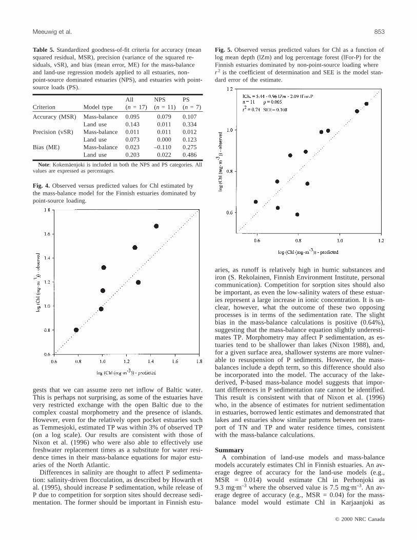
Finnish Chl–TP equation (Table 3). The MSR for Chl esti-mated from the mass-balance approach was 0.095 (Table 5;Fig. 4).

Estimating Chl from land useNo significant relationships existed between Chl and land-

use variables for 17 estuaries (two of the 19 estuaries weremissing morphometric data and thus could not be includedin the land-use models). However, land-use models primarilycapture non-point-source human influences, and of the 17estuaries, seven had significant municipal or industrial pointsources immediately on the shore of the estuary that werenot included in the riverine nutrient load estimates. We thustemporarily removed these estuaries, hence referred to aspoint-source (PS) estuaries, from the data set. The remaining10 estuaries, hence referred to as non-point-source (NPS) es-tuaries, then formed the core data set for the land-use regres-sion modeling. A number of significant regression modelswere then generated. Of these models, the model estimatinglog Chl (lChl) as a function of log mean depth (lZm) and logpercentage of the catchment forested (lFor-P) had the high-est coefficient of determination and lowest model standarderror. Both partial regression coefficients were also signifi-cant (p < 0.05). We then added the PS estuaries to the modelto see which fit the same pattern. Of the seven PS estuaries,only Kokemäenjoki did not substantially decrease the modelcoefficient of determination or increase the model standarderror when included. Moreover, its inclusion did not signifi-

© 2000 NRC Canada

Meeuwig et al. 849

Urb-P Ag-P For-PWshed(km2)

Pden(km–2)

TPL-R(t·year–1)

TPL-D(t·year–1)

TNL-R(t·year–1)

TNL-D(t·year–1) Ratio

0.5 13.5 82.9 357 9.6 7.0 3.0 242 23.6 300.8 14.0 80.7 380 28.3 9.4 2320.4 15.3 82.4 569 24.3 14.1 3483.8 22.8 70.1 989 80.4 259.8 6 8580.7 23.1 73.4 309 36.02.4 28.5 67.9 1273 64.7 50.8 12.8 1609 73.6 201.3 26.8 70.7 783 30.5 20.4 1.8 468 91.0 82.5 32.3 64.8 220 46.9 5.3 1316.7 23.6 67.7 1686 265.1 53.4 1 4532.8 29.9 65.3 116 37.8 26.8 1.3 683 45.4 52.0 34.0 63.6 764 33.4 43.2 0.9 501 84.4 21.2 43.0 54.3 1088 17.7 80.8 9521.5 33.0 65.4 284 28.3 15.3 2241.2 19.0 78.6 685 14.0 15.5 2271.4 27.0 67.7 6817 26.4 446.6 20.0 10 433 337.4 40.7 20.6 78.0 992 21.1 3691.0 23.3 74.3 4923 20.0 163.2 3 2150.3 9.5 87.2 2524 11.7 66.0 8280.4 15.4 83.6 1181 9.0 28.1 431

1.7 24.5 72.6 1365 43.6 73.7 6.6 1 623 109.2 121.54 8.36 8.59 1719 58.3 113.0 7.9 2 730 114.6 11.10.35 9.50 54.34 116 9.0 5.3 0.9 131 23.6 2.06.73 42.97 87.16 6817 265.1 446.6 20.0 10 433 337.4 30.0



cantly affect the regression coefficients. Given the small sizeof the data set available for the regression modeling, weincluded Kokemäenjoki in the regression model. The bestland-use model is thus

(8) lChl = 5.44 – 0.96 lZm – 2.09 lFor-P

with n = 11, p = 0.005, r 2 = 0.74, and model standarderror = 0.108. (Fig. 5). One must be cautious in estimatingthree parameters from a sample size of 11. However, bothpvalues for the partial regression coefficients were significant

(p = 0.0014 for lZm andp = 0.01 for lFor-P), and thecoefficient of determination sums to more than the individ-ual coefficients of determination (r 2 = 0.44 for lZm andr 2 =0.01 for lFor-P). Thus, the model coefficients are likely ro-bust.

Comparing the accuracy of Chl estimates from themass-balance and land-use models

We compared the accuracy, precision, and bias of the Chlestimates generated via the mass-balance model and theland-use model for all the estuaries, the NPS estuaries, andthe PS estuaries (with Kokemäenjoki included in bothgroups) (Table 5). When considering all the estuaries, the es-timates of Chl via the mass-balance model were more accu-rate and precise and less biased than the estimates from theland-use model. Accuracy (MSR) was 0.095 when the mass-balance model was used as opposed to 0.143 with the land-use model. Precision (vSR) was 0.011 and 0.073, respec-tively, and bias (ME) was 0.023 and 0.203, respectively. Thepositive bias value for the land-use model suggests that ittends to underestimate observed Chl.

The most accurate, precise, and unbiased estimates are tobe achieved by separating the estuaries into NPS and PSgroups (Table 5). The land-use model most accurately andprecisely estimates Chl for the NPS estuaries, with an MSRand vSR of 0.011 and 0, respectively. Bias is only 0.022. Ifthe mass-balance is used to estimate Chl in the NPS estuar-ies, the MSR and vSR increase to 0.079 and 0.011, respec-tively, and bias increases to –0.11. This can only partially beattributed to the poor estimate of TP for Perhonjoki (forwhich it was difficult to estimate TP), as its removal only re-duced the MSR to 0.68. The mosta ccurate, precise, and un-biased estimates of Chl for the PS estuaries were generatedby the mass-balance model. The MSR is 0.107, which issubstantially smaller than the MSR of 0.334 for the esti-mates based on the land-use model.

Discussion

Predicting coastal eutrophication in Finnish estuariesThe above analyses demonstrate the applicability of re-

gression and P mass-balances to Finnish estuaries. We haveshown that regression models based on single nutrients orland use can be fit to data from Finnish estuaries and that ex-isting P mass-balance models such as that of Canfield andBachmann (1981) accurately estimate TP. The approach did,however, require the division of the estuaries into twogroups: those dominated by point-source loading and thosedominated by non-point-source loading. Based on the rela-tive goodness-of-fit, the analysis suggests the followingguidelines for model choice in predicting Chl: (i) for estuar-ies dominated by non-point-source loading (ratio of PS loadto total load <0.01), Chl is best estimated by the land-use re-gression model and (ii ) for estuaries receiving point-sourceloading greater than 1% of the total load, Chl is best esti-mated by the mass-balance model. These guidelines and theland-use model itself must still be tested. Chl should be pre-dicted for estuaries not included in this analysis using boththe land-use regression and the mass-balance. The relativeaccuracy of the predictions can then be compared along withtheir correspondence to the above guidelines. To this end,

© 2000 NRC Canada


Fig. 2. Regression equations for Chl as a function of TP and Chlas a function of TN for the 19 estuaries wherer 2 is the coeffi-cient of determination and SEE is the model standard error ofthe estimate.



we have made the guidelines quantitative to reduce ambigu-ity as to which model should perform best.

It may be that the above guidelines reflect quirks in thepresent set of data rather than any general patterns in the ap-plicability of the land-use model, particularly as it was de-veloped on a small number of observations. In this case, themost conservative position would predict Chl via the mass-balance. Such predictions should still be within 10% of ob-served values and thus represent more predictive power thanyet exists for Finnish estuaries. The mass-balance estimatesare also true predictions in that an existing mass-balancemodel was applied to these data rather than fitting a new one.

It is admittedly dangerous to subdivide one’s data until“accurate” predictions are attained. A division between PSand NPS estuaries does, however, seem reasonable. This di-vision likely reflects the different sources and thus composi-tion of TP in PS and NPS estuaries. In the PS estuaries,there are generally two sources of TP: point-source TP de-rived from municipal and industrial activities and, in onecase, fish farms, and non-point-source TP derived primarilyfrom agricultural activities in the catchment. In the NPSestuaries, the majority of TP is derived from agricultural ac-tivity (Rekolainen et al. 1995). TP from municipal wastescontains a greater proportion of bioavailable P than TP de-rived from agricultural sources (Ekholm 1994). In addition,the point sources are proximate to the estuaries comparedwith non-point-source TP, which is derived from the entirecatchment. The combination of a greater proportion of bio-available P and its rapid delivery to the estuary may explainwhy the mass-balance model performs better than the land-use model in the PS estuaries. The land-use model givesequal weight to all disturbance, regardless of proximity tothe estuary, and thus emphasizes diffuse disturbance. The ef-fect is also likely exaggerated in these estuaries, which havea relatively large catchment to surface area ratio (>70). Thisanalysis indicates the importance of considering both the na-ture of the sources and their spatial distribution.

Coastal limnology: Finnish estuaries as salty lakesEutrophication tradition emphasizes the differences be-

tween lakes and estuaries (Richardson and Jørgensen 1996).Lakes and estuaries differ in water residence time, waterchemistry, turbidity, grazing, morphometry, physical energy,and limiting nutrients. Whether these differences translateinto differential eutrophication response to nutrients and

anthropogenic disturbance is unclear, however. Finnish estu-aries share characteristics of both lakes and estuaries: likelakes, they are nontidal, and like estuaries, they are opensystems. They are, however, intermediate in terms of salin-ity. They thus provide an interesting test case for both lim-nological approaches and a test case of whether theeutrophication responses are quantitatively similar.

Our results suggest that mass-balance and regression ap-proaches can in fact be applied to estuaries such as those inFinland. Our results also show that eutrophication responsesin lakes and Finnish estuaries are quantitatively similar, atleast with respect to Chl–TP equations (Table 3; Fig. 3) andthe mass-balance equation. This is perhaps not surprising. Inthe case of the Chl–TP equation, we have to consider thatphytoplankton have similar elemental composition and re-quirements in both systems (Hecky and Kilham 1988); thus,the Chl–TP yield should be similar. Water residence timeand morphometry should have little effect on Chl–TP yields,as one would not expect differential dilution of these compo-nents. For instance, Basu and Pick (1996) developed regres-sion models predicting Chl as a function of TP in rivers withresidence times as short as 3 days. Water chemistry could af-fect the Chl–TP yield if the bioavailability of TP changed.However, both removal of P via flocculation at low salinity(2–3 ppt) (Howarth et al. 1995) and release of P throughcompetition for sorption sites when river and seawater meetstill allow for corresponding decreases or increases in Chl.

Of the cited differences between freshwater and coastalsystems, turbidity, herbivory, and P versus N limitation maychange the Chl–TP yield. Light limitation reduces the yieldof Chl as phytoplankton are unable to take advantage ofavailable P (Fisher et al. 1995). However, light limitation oc-curs primarily in permanent turbidity maxima that, to ourknowledge, have not been documented in Finnish estuaries.Herbivory has also been shown to decrease Chl yields(Mellina et al. 1995; Meeuwig et al. 1998). The zoobenthosof Finnish estuaries includes phytoplanktivores such asMacoma balthicaandMytilus edulis(Lax et al. 1993). How-ever, although abundance of bivalves has increased in gen-eral in the Baltic (Cederwall and Elmgren 1980), inshoreareas show declines due to pollution and hypoxia (Mattila1993). The Chl–TP yield also changes as a function of Pversus N limitation. For instance, Prairie et al. (1989) dem-onstrated systematic changes in the regression coefficientswith changing N:P ratios that they interpreted as indicatingchanges in P versus N limitation. However, although theouter waters of the Baltic are thought to be primarily N lim-ited (Wulff et al. 1990), the estuaries are considered to beprimarily P limited (Pitkänen and Tamminen 1994), thussuggesting that the yields should be similar to those seen inP-limited lakes.

It is not surprising that a lake-derived, P-based mass-balance model can be applied to these estuaries. First, we donot really know whether estuaries are N or P limited; N ver-sus P limitation in estuaries remains an issue of some con-tention, despite the dogma of N limitation. Hecky andKilham (1988) reviewed the evidence for N versus P limita-tion in coastal waters; they argued that the evidence for Nlimitation at an ecosystem level was weak, given the lack oflarge-scale experiments and comparative data. These gaps inempirical or experimental evidence remain. Further, Elser et

© 2000 NRC Canada

Meeuwig et al. 851

Equation r 2 n

Finnish estuaries lChl = –1.03 + 1.26 lTP 0.67 19Lakes (OECD 1982) lChl = –0.55 + 0.96 lTP 0.88 77Lakes (Dillon and

Rigler 1974)lChl = –1.14 + 1.45 lTP 0.96 77

Finnish estuaries lChl = –2.10 + 1.13 lTN 0.53 19Lakes (Sakamoto

1966)lChl = –2.5 + 1.4 lTN nr 21

Lakes (Prairie et al.1989)

lChl = –3.13 + 1.45 lTN 0.69 133

Note: All variables transformed to log10 (l). r 2, coefficient of determination;n, sample size; nr, not reported.

Table 3. Comparison of the Chl–TP and Chl–TN regression equa-tions in Finnish estuaries and lakes.



al. (1990) reviewed the evidence for single nutrient limita-tion in whole-lake experiments and argued that colimitationwas more likely the norm at the scale of whole ecosystems.Indeed, we have argued that this is the case in lakes(Meeuwig and Peters 1996) and eastern Canadian estuaries(Meeuwig 1999) and where land-use models account for agreater proportion of the variance. Finally, as N and Pcovary, P can be viewed as a surrogate for N if the idea of Por colimitation remains too uncomfortable.

The mass-balance also likely works because differencesbetween lakes and estuaries are incorporated into the modelvia variables such as water residence time and P sedimenta-tion. Differences in physical energy and morphometry thatresult in shorter residence times in coastal systems are ad-dressed by the water residence time. When the estuarieswere treated as lakes and residence time calculated onlyfrom river freshwater load, estimated log TP values werewithin 9.7% of observed log TP values on average. This sug-

© 2000 NRC Canada


Estuarycode

ObservedTP (mg·m–3)

TP-FW(mg·m–3)

TP-B(mg·m–3)

Rt-FW(months)

Rt-B(months)

11 46.9 32.4 9.7 14.71 2.0512 46.8 39.1 6.8 6.16 0.5713 35.3 58.1 5.5 0.66 0.0514 39.3 22.0 9.9 0.29 0.1217 28.018 66.6 44.5 18.0 16.81 2.8519 36.0 33.0 9.7 26.65 2.8120 59.9 51.1 17.0 1.33 0.3321 91.2 53.3 3.4023 23.0 19.7 15.8 18.23 11.7026 65.9 39.4 28.7 42.73 14.4627 28.2 32.0 11.0 98.10 6.0429 33.7 39.5 9.2 31.76 2.0530 34.9 33.5 16.5 50.51 7.9835 39.1 49.7 34.5* 0.15 0.1039 20.0 31.1 3.1 7.89 0.4042 92.249 20.2 71.5 17.4* 0.48 0.0958 37.8 34.1 15.6 8.36 2.34

Note: Estuaries where TP is better estimated via Bowden’s equation are indicated with an asterisk.

Table 4. Comparison of observed TP to TP calculated using water residence times calculated as freshwa-ter replacement time (TP-FW, Rt-FW) and via Bowden’s (1980) saltwater fraction method (TP-B, Rt-B).

Fig. 3. Frequency histogram of slopes and intercepts for Chl–TP equations in the literature (J.J. Meeuwig, unpublished data).



gests that we can assume zero net inflow of Baltic water.This is perhaps not surprising, as some of the estuaries havevery restricted exchange with the open Baltic due to thecomplex coastal morphometry and the presence of islands.However, even for the relatively open pocket estuaries suchas Temmesjoki, estimated TP was within 3% of observed TP(on a log scale). Our results are consistent with those ofNixon et al. (1996) who were also able to effectively usefreshwater replacement times as a substitute for water resi-dence times in their mass-balance equations for major estu-aries of the North Atlantic.

Differences in salinity are thought to affect P sedimenta-tion: salinity-driven flocculation, as described by Howarth etal. (1995), should increase P sedimentation, while release ofP due to competition for sorption sites should decrease sedi-mentation. The former should be important in Finnish estu-

aries, as runoff is relatively high in humic substances andiron (S. Rekolainen, Finnish Environment Institute, personalcommunication). Competition for sorption sites should alsobe important, as even the low-salinity waters of these estuar-ies represent a large increase in ionic concentration. It is un-clear, however, what the outcome of these two opposingprocesses is in terms of the sedimentation rate. The slightbias in the mass-balance calculations is positive (0.64%),suggesting that the mass-balance equation slightly underesti-mates TP. Morphometry may affect P sedimentation, as es-tuaries tend to be shallower than lakes (Nixon 1988), and,for a given surface area, shallower systems are more vulner-able to resuspension of P sediments. However, the mass-balances include a depth term, so this difference should alsobe incorporated into the model. The accuracy of the lake-derived, P-based mass-balance model suggests that impor-tant differences in P sedimentation rate cannot be identified.This result is consistent with that of Nixon et al. (1996)who, in the absence of estimates for nutrient sedimentationin estuaries, borrowed lentic estimates and demonstrated thatlakes and estuaries show similar patterns between net trans-port of TN and TP and water residence times, consistentwith the mass-balance calculations.

SummaryA combination of land-use models and mass-balance

models accurately estimates Chl in Finnish estuaries. An av-erage degree of accuracy for the land-use models (e.g.,MSR = 0.014) would estimate Chl in Perhonjoki as9.3 mg·m–3 where the observed value is 7.5 mg·m–3. An av-erage degree of accuracy (e.g., MSR = 0.04) for the mass-balance model would estimate Chl in Karjaanjoki as

© 2000 NRC Canada

Meeuwig et al. 853

Fig. 5. Observed versus predicted values for Chl as a function oflog mean depth (lZm) and log percentage forest (lFor-P) for theFinnish estuaries dominated by non-point-source loading wherer 2 is the coefficient of determination and SEE is the model stan-dard error of the estimate.

Fig. 4. Observed versus predicted values for Chl estimated bythe mass-balance model for the Finnish estuaries dominated bypoint-source loading.

Criterion Model typeAll(n = 17)

NPS(n = 11)

PS(n = 7)

Accuracy (MSR) Mass-balance 0.095 0.079 0.107Land use 0.143 0.011 0.334

Precision (vSR) Mass-balance 0.011 0.011 0.012Land use 0.073 0.000 0.123

Bias (ME) Mass-balance 0.023 –0.110 0.275Land use 0.203 0.022 0.486

Note: Kokemäenjoki is included in both the NPS and PS categories. Allvalues are expressed as percentages.

Table 5. Standardized goodness-of-fit criteria for accuracy (meansquared residual, MSR), precision (variance of the squared re-siduals, vSR), and bias (mean error, ME) for the mass-balanceand land-use regression models applied to all estuaries, non-point-source dominated estuaries (NPS), and estuaries with point-source loads (PS).



4 mg·m–3 where the observed value is 6 mg·m–3. This degreeof accuracy suggests that the mass-balance approach andother limnological models such as the land-use regressioncan effectively estimate coastal eutrophication in Finnish es-tuaries. It remains, however, to test the predictive power ofthese models on estuaries not used in their development.

This analysis also demonstrates that Finnish estuaries andlakes respond similarly to total nutrients and nutrient loads.Finnish estuaries are not typical estuaries, however, as theyare essentially nontidal and have lower salinity than mostestuaries. It thus remains to be demonstrated whether themass-balance approach can be effectively applied to the es-tuaries of North America and Atlantic Europe.

Acknowledgements

This study would have been impossible without the hospi-tality of the Finnish Environment Institute and the extensivedata set that they meticulously collect and maintain. We aregrateful for the help of Anu Hakala, Yki Laine, Kati Manni,and Mika Ristimäki in compiling the data, and we thankPetri Ekholm and Seppo Rekolainen for their insights into Pexport. This research was supported by a CIMO research fel-lowship to J.J.M. and is a contribution from the McGill Lim-nology Research Center.

References

Basu, B., and Pick, F. 1996. Factors regulating phytoplankton andzooplankton biomass in temperate rivers. Limnol. Oceanogr.41:1572–1577.

Bonsdorff, E., Blomqvist, E.M., Mattila, J., and Norkko, A. 1997.Coastal eutrophication: causes, consequences and perspectivesin the Archipelago areas of the northern Baltic Sea. EstuarineCoastal Shelf Sci.44(Suppl. A): 63–72.

Bowden, K.F. 1980. Physical factors: salinity temperature circula-tion and mixing processes.In Chemistry and biogeochemistry ofestuaries.Edited by E. Olausson and I. Cato. John Wiley &Sons, Chichester, U.K. pp. 37–70.

Canfield, D.R., and Bachmann, R.W. 1981. Prediction of total phos-phorus concentrations, chlorophyll-a, and Secchi depths in naturaland artificial lakes. Can. J. Fish. Aquat. Sci.38: 414–423.

Cederwall, H., and Elmgren, R. 1980. Biomass increase of benthicmacrofauna demonstrates eutrophication of the Baltic Sea.Ophelia Suppl.1: 287–304.

Dillon, P.J., and Rigler, F.H. 1974. The phosphorus–chlorophyll re-lationship in lakes. Limnol. Oceanogr.19: 767–773.

Ekholm, P. 1994. Bioavailability of phosphorus in agriculturallyloaded rivers in southern Finland. Hydrobiologia,287: 179–194.

Elser, J.J., Marzolf, E.R., and Goldman, C.R. 1990. Phosphorusand nitrogen limitation of phytoplankton growth in freshwatersof North America: a review and critique of experimental enrich-ments. Can. J. Fish. Aquat. Sci.47: 1468–1477.

Finnish Environment Institute. 1998. Database of the monitoringsystem of spatial structure in major Finnish urban regions. Finn-ish Environment Institute, Helsinki, Finland.

Finnish Institute of Navigation. 1996–1998. Merenkulkulaitos Kartta[sea charts]. Vols. A, B, D, E, F, and G. Finnish Institute of Navi-gation, Helsinki, Finland.

Fisher, T.R., Melack, J.M, Grobbelaar, J.U., and Howarth R.W. 1995.Nutrient limitation of phytoplankton and eutrophication of inland,estuarine, and marine waters.In Phosphorus in the global environ-

ment.Edited byH. Tiessen. John Wiley & Sons, Chichester, U.K.pp. 301–322.

Hecky, R.E., and Kilham, P. 1988. Nutrient limitation of phyto-plankton in freshwater and marine environments: a review of re-cent evidence on the effects of enrichment. Limnol. Oceanogr.33(4/2): 796–822.

HELCOM. 1997. Third periodic assessment of the state of the ma-rine environment of the Baltic Sea, 1989–1993. Backgrounddocument. Baltic Sea Environment Proc. No. 64B. HELCOM –Baltic Marine Environment Protection Commission – HelsinkiCommission, Helsinki, Finland.

Howarth, R.W., Jensen, H.S., Marino, R., and Postma, H. 1995.Transport to and processing of P in near-shore and oceanic wa-ters. In Phosphorus in the global environment.Edited by H.Tiessen. John Wiley & Sons, Chichester, U.K. pp. 323–343.

Lapointe, B.E., and Clark, M.W. 1992. Nutrient inputs from thewatershed and coastal eutrophication in the Florida Keys. Estu-aries,15: 465–476.

Lax, H.G., Kangas, P., and Storgård-Envall, C. 1993. Spatio-temporalvariations of sedimentation and soft bottom macrofauna in thecoastal waters of the Gulf of Bothnia. Aqua Fenn.23: 177–186.

Mattila, J. 1993. Long-term changes in the bottom fauna along theFinnish coasts of the southern Bothnian Sea. Aqua Fenn.23:143–152.

Meeuwig, J.J. 1999. Predicting coastal eutrophication from land-use: an empirical approach to small non-stratified estuaries. Mar.Ecol. Prog. Ser.176: 231–241.

Meeuwig, J.J., and Peters, R.H. 1996. Circumventing phosphorusin lake management: a comparison of chlorophylla predictionsfrom land-use and phosphorus-loading models. Can. J. Fish.Aquat. Sci.53: 1795–1806.

Meeuwig, J.J., Rasmussen, J.B., and Peters, R.H. 1998. Turbid wa-ters and clarifying mussels: their moderation of Chl:nutrient re-lations in estuaries. Mar. Ecol. Prog. Ser.171: 139–150.

Mellina, E., Rasmussen, J.B., and Mills, E.L. 1995. Impact of ze-bra mussels (Dreissena polymorpha) on phosphorus cycling andchlorophyll in lakes. Can. J. Fish. Aquat. Sci.52: 2553–2579.

National Board of Waters. 1981. Vesihallinnon analyysimenetelmät[Analytical methods used by the Finnish Water Authority]. Rep.213. National Board of Waters, Helsinki, Finland.

Nehring, D. 1992. Eutrophication in the Baltic Sea. Sci. Total En-viron. Suppl. pp. 673–682.

Nixon, S.W. 1988. Physical energy inputs and the comparativeecology of lake and marine ecosystems. Limnol. Oceanogr.33(4/2): 1005–1025.

Nixon, S.W., Ammerman, J.W., Atkinson, L.P., Berounsky, V.M.,Billen, G., Boicourt, W.C., Boynton, W.R., Church, T.M., Ditoro,D.M., Elmgren, R., Garber, J.H., Giblin, A.E., Jahnke, R.A.,Owens, N.J.P., Pilson, M.E.Q., and Seitzinger, S.P. 1996. The fateof nitrogen and phosphorus at the land–sea margin of the NorthAtlantic Ocean. Biogeochemistry,35: 141–180.

OECD. 1982. Eutrophication of waters: monitoring, assessmentand control. OECD, Paris.

Pitkänen, H. 1994. Eutrophication of the Finnish coastal waters:origin, fate and effects of riverine nutrient fluxes. Publ. WaterEnviron. Res. Inst. No. 18.

Pitkänen, H., and Tamminen, T. 1994. Nitrogen and phosphorus asproduction limiting factors in the estuarine waters of the easternGulf of Finland. Mar. Ecol. Prog. Ser.129: 283–294.

Prairie, Y.T., Duarte, C.M., and Kalff, J. 1989. Unifying nutrient–chlorophyll relationships in lakes. Can. J. Fish. Aquat. Sci.46:1176–1182.

Rekolainen, S., Pitkänen, H., Bleeker, A., and Sietske, F. 1995. Ni-

© 2000 NRC Canada




trogen and phosphorus fluxes from Finnish agricultural areas tothe Baltic Sea. Nord. Hydrol.26: 55–72.

Richardson, K., and Jørgensen, B.B. 1996. Eutrophication: defini-tion, history and effects.In Eutrophication in coastal marine eco-systems.Edited byK. Richardson and B.B. Jørgensen. CoastalEstuarine Stud.52: 1–19.

Rosenberg, R., Elmgren, R., Fleischer, S., Jonsson, P., Persson, G.,and Dahlin, H. 1990. Marine eutrophication case studies in Swe-den. Ambio,19: 102–108.

Sakamoto, M. 1966. Primary production by phytoplankton commu-nity in some Japanese lakes and its dependence on lake depth.Arch. Hydrobiol. 62: 1–28.

Schaub, B.E.M., and Gieskes, W.W.C. 1991. Trends in eutrophicationof Dutch coastal waters: the relation between Rhine river discharge

and chlorophyll-a concentrations.In Estuaries and coasts: spatialand temporal intercomparisons.Edited by M. Elliott and J.P.Ducrotoy. Olsen and Olsen, Fredensborg. pp. 85–90.

Vollenweider, R.A. 1975. Input–output models with special refer-ence to the phosphorus loading concept in limnology. Schweiz.Z. Hydrol. 37: 53–84.

Walling, B.E., and Webb, B.W. 1985. Estimating the discharge ofcontaminants to coastal waters by rivers: some cautionary com-ments. Mar. Pollut. Bull.16: 488–492.

Wulff, F., Stigebrandt, A., and Rahm, L. 1990. Nutrient dynamicsof the Baltic Sea. Ambio,19: 126–133.

Zar, J.H. 1984. Biostatistical analysis. Prentice-Hall, EnglewoodCliffs, N.J.

© 2000 NRC Canada

Meeuwig et al. 855



Documents

Predicting coastal eutrophication in the Baltic: a limnological approach