Predicting Product Returns in E-Commerce

Tos Sambo

August 14, 2018

Abstract

Product returns are currently a major complication for online retailers that severelyaffect overall profits, especially in the apparel sector. In order to minimize the costsassociated with product returns, it is not only important for online retailers to un-derstand what drives customers to return purchases, but also to know which productpurchases are likely to be returned. In this study, we therefore examine whetheran ensemble selection prediction model is able to accurately predict product re-turns based on customer-, product- and shopping basket characteristic. In addition,we explore the correlation between these particular characteristics and the returnprobability. Using a large data set containing purchases from a major Dutch on-line retailer, we demonstrate that our proposed ensemble selection prediction modelcan predict product return rates at sufficient accuracy to benefit online retailers intheir pursuit to minimize product return costs. We also show that our ensembleoutperforms a wide selection of state-of-the-art classification algorithms in severalways, where most algorithms of this selection are able to predict product returnseffectively as well. Furthermore, we show how return decisions are influenced bycustomer-, product-, and return shopping basket characteristics. It turns out thatimportant factors influencing the return probability are, amongst others, gender andage, product price and -quality, and the number of different product categories inthe basket.

Keywords: Product returns, e-commerce, online retail, customer-, product andshopping basket characteristics, statistical methods, ensemble selection predictionmodel, machine learning

Contents

Page

Introduction 3

Literature Review 5Predictive analytics in product returns . . . . . . . . . . . . . . . . . . . . . . . 5Variables to complement predictive models of product returns . . . . . . . . . . 7

Customer related variables . . . . . . . . . . . . . . . . . . . . . . . . . . . 8Product related variables . . . . . . . . . . . . . . . . . . . . . . . . . . . 8Shopping basket related variables . . . . . . . . . . . . . . . . . . . . . . . 9

Data Description 10

Methodology 13Explanatory model . . . . . . . . . . . . . . . . . . . . . . . . . . . . . . . . . . 14Predictive models . . . . . . . . . . . . . . . . . . . . . . . . . . . . . . . . . . . 16

Validation measures . . . . . . . . . . . . . . . . . . . . . . . . . . . . . . 17Overall performance . . . . . . . . . . . . . . . . . . . . . . . . . . 19Calibration and discrimination . . . . . . . . . . . . . . . . . . . . 20Practical usefulness . . . . . . . . . . . . . . . . . . . . . . . . . . 21

Results 21Explaining product returns . . . . . . . . . . . . . . . . . . . . . . . . . . . . . 21

Customer characteristics . . . . . . . . . . . . . . . . . . . . . . . . . . . . 24Product characteristics . . . . . . . . . . . . . . . . . . . . . . . . . . . . . 24Shopping basket characteristics . . . . . . . . . . . . . . . . . . . . . . . . 25Control variables . . . . . . . . . . . . . . . . . . . . . . . . . . . . . . . . 26

Predicting product returns . . . . . . . . . . . . . . . . . . . . . . . . . . . . . 27Overall performance . . . . . . . . . . . . . . . . . . . . . . . . . . . . . . 28Calibration and discrimination . . . . . . . . . . . . . . . . . . . . . . . . 29Practical usefulness . . . . . . . . . . . . . . . . . . . . . . . . . . . . . . . 30

Conclusion and Discussion 31Theoretical conclusions . . . . . . . . . . . . . . . . . . . . . . . . . . . . . . . 32Practical implications . . . . . . . . . . . . . . . . . . . . . . . . . . . . . . . . 32Limitations . . . . . . . . . . . . . . . . . . . . . . . . . . . . . . . . . . . . . . 33Recommendations . . . . . . . . . . . . . . . . . . . . . . . . . . . . . . . . . . 33

References 34

Appendix 37Individual algorithms . . . . . . . . . . . . . . . . . . . . . . . . . . . . . . . . 37

Adaptive Boosting . . . . . . . . . . . . . . . . . . . . . . . . . . . . . . . 37Extreme Gradient Boosting . . . . . . . . . . . . . . . . . . . . . . . . . . 37k Nearest Neighbors . . . . . . . . . . . . . . . . . . . . . . . . . . . . . . 38Logistic Regression . . . . . . . . . . . . . . . . . . . . . . . . . . . . . . . 39Multilayer Perceptron . . . . . . . . . . . . . . . . . . . . . . . . . . . . . 39Naive Bayes . . . . . . . . . . . . . . . . . . . . . . . . . . . . . . . . . . . 40Support Vector Machine . . . . . . . . . . . . . . . . . . . . . . . . . . . . 41Random Forest . . . . . . . . . . . . . . . . . . . . . . . . . . . . . . . . . 42

All logistic regression results . . . . . . . . . . . . . . . . . . . . . . . . . . . . 43

2

Introduction

Ever since the beginning of the digital age, engaging in e-commerce has been the path to

retail success for many small as well as more substantial retailers. However, selling online

does not in itself guarantee success and comes with a host of challenges and costs. The

costs of product returns, for example, is a rather considerable expense line that e-commerce

retailers have to take into account. It has been estimated that worldwide product re-

turns reduce retailers’ profits by 3.8% on average each year (David, 2007). It should therefore

not come as a surprise that e-commerce retailers pursue the minimization of product return costs.

In general, there are two strategies online retailers can employ to minimize the costs as-

sociated with product returns, namely, what is called ‘value creation’ and ‘cost reduction’

(Bijmolt et al., 2017). Value creation in this instance focuses on product value recovery and

creating Customer Lifetime Value (CLV), considering an operations- and marketing approach

respectively. Cost reduction with an operations approach, on the other hand, concentrates on

the optimization of processes to minimize return costs, while cost reduction with a marketing

approach focuses on reducing the return rate of customers.

While this may give the impression that e-commerce retailers employing counter mea-

sures to reduce the product return costs attempt to achieve return rates of zero by all means,

that is not entirely true. That is to say because retailers also realize that customers desire

high-quality service, including the possibility to return products. Providing this high-quality

service, and thus the possibility to return products, enhances the relationship with customers

(Stock et al., 2002) and in that way may increase purchase rates (Wood, 2001); something

retailers generally celebrate. Depending on the leniency of a return policy, which may also

positively affect the future purchasing behavior of customers, a moderate amount of product

returns may even maximize profits (Petersen and Kumar, 2009). In other words, there exists an

optimal return rate that balances the costs associated with product returns and the beneficial

impact of providing a lenience return policy.

In order to find this optimal return rate and minimize product return costs, it is impor-

tant for e-commerce retailers to understand what drives the proportion of returns, which

customers can be classified as return-prone customers and, most importantly, which products

are likely to be returned. Having such information can benefit online retailers in their decision

making and action taking in relation to product returns.

For instance, accurate prediction of a customer’s likelihood to return a product can help

in customer management and determining optimal marketing resource allocation; return-prone

customers, for example, can be identified and might be excluded from marketing allocation.

Alternatively, correctly predicting product returns can move online retailers to take return-

discouraging actions against such customers by, for example, using moral suasion. Knowing that

environmental awareness can effectively influence customer behavior (Aguilar and Cai, 2010;

D’Souza et al., 2006; Bjørner et al., 2004), an online retailer could remind customers of the

environmental impact associated with product returns by using pop-ups.

3

Hence, for e-commerce retailers to approximate the optimal return rate and minimize the

associated costs, accurately predicting the likelihood of product returns is essential. Although

all recognize the necessity of this, most find it hard to make such predictions, and consequently,

are not able to account for product returns in their return management.

Several methods can be applied in order to predict a certain outcome. Probably the most

common prediction method is the logistic regression. However, other classification algorithms

such as neural networks, support vector machines or the k Nearest Neighbor have also been

demonstrated to be successful across a large variety of problem domains (Fernandez-Delgado

et al., 2014).

In addition, there exist more advanced techniques that could predict a certain outcome, such

as ensemble modeling. The principle of ensemble modeling is to combine multiple predictive

models, or so called candidate models, together. Taking multiple predictions of different models

into account makes a final prediction generally more accurate and consistent and decreases the

bias. Previous studies in other domains have indeed evidenced the efficacy of ensemble modeling

(Tsoumakas et al., 2008; Lessmann and Voß, 2010), but more important, ensemble models have

also been shown to be effective in predicting product returns (Heilig et al., 2016; Urbanke et al.,

2015).

Therefore, the goal of this study is to examine if an ensemble selection prediction model

based on customer-, product- and shopping basket specific characteristics yields an efficient

prediction of a product return, and in that way potentially provide the online retailers with a

useful model that can support their decision making related to product returns. Efficient, in

this study, refers to 4 specific model validity aspects, namely, overall performance, calibration,

discrimination and practical usefulness, which are explained in full detail later on in this study.

Ultimately, this study’s aim is to answer the following question:

Is an ensemble selection prediction model based on customer-, product- and shopping basket

specific characteristics able to efficiently predict product returns, so that the model is useful to

support decision making processing related to product returns?

In order to understand the efficiency of our proposed ensemble selection model, it is important

to separately examine the performance of each individual prediction model as well. Therefore,

this study will also answer the following two sub-questions:

Is each of the individual prediction able to efficiently predict product returns based on customer-,

product- and shopping basket specific characteristics?

Is our proposed ensemble selection model more efficient in predicting product returns, as

compared to each individual prediction model?

Moreover, to get more insight in the dynamics behind the predictions, this study also investigates

the effect of customer-, product- and shopping basket specific characteristics on product returns

by answering the last sub-question:

How are product returns influenced by customer-, product- and shopping basket specific

characteristics?

4

Data of a major Dutch online retailer that sells heterogeneous product categories exclusively

through its online store is used to answer the above stated questions.

In order of sequence, this paper discusses the existing literature on product returns in

the section Literature Review. The sections Data Description and Methodology then describe

the outline of the performed data-analysis in more detail, starting with summary statistics of

the dataset, and explain the methods conducted to translate the used data into the models

of interest. The section Results follows, discussing the results of the models in full detail.

Namely, the results of our study suggest that an ensemble selection prediction model based

on customer-, product-, and basket level characteristics is able to predict product returns

at sufficient accuracy, where we also demonstrate its business value. Ultimately, our study

concludes, in section Conclusion and Discussion, that although an ensemble may not be the

best choice of prediction model to use in practice, under certain circumstances, it could benefit

online retailers in reducing product returns and increasing profit margins. In the same section

the limitations and suggestions for further research are discussed.

Literature Review

The substantial financial impact of product returns on the profits of online retailers has prompted

academic research on product returns. A large number of studies has been done and the existing

literature covers a wide variety of theories on this topic; from theories on the antecedents and

consequences of product returns to supply chain complexities. Surprisingly, literature related to

product return prediction specifically, is scarce.

Therefore, we deem additional research into predicting product returns important. It

may not only further benefit online retailers in streamlining their businesses, but may benefit

online customers and the broader society as well. For customers, effective product return

predictions might indicate whether a particular item has a high probability of fit for them or

not, averting unnecessary bad buys and wrongly spent finances. The broader society could also

benefit from an accurate prediction model, not only economically, but also ecologically. That is

to say because accurately predicting product returns, and, if acted upon, the resulting reduced

return rates, need less material used in product packaging. In turn, this reduces the volume

of waste sent to landfills, next to many other environmental benefits of a reduced amount of

product returns.

Predictive analytics in product returns

Although there is no abundance of literature related to product return prediction, the importance

of such studies has been recognized and various statistical methods to address the issue of product

returns have been suggested. Toktay (2001), in his book “Forecasting Product Returns”, for

example, describes several time-series forecasting methods to forecast return volumes which are

particularly relevant for inventory management and production planning.

Yu and Wang (2008) in their article “A hybrid mining approach for optimizing returns policies

in e-retailing”, on the other hand, propose a hybrid mining approach to analyze return patterns,

to classify customers and products with return ratios, as well as to direct suitable return policies

and marketing strategies to specific customer and product classes. In other words, their approach

5

is to divide customers into different segments to which, in turn, different return policies are offered

to.

Even though we recognize that the methods proposed by Toktay, and Yu and Wang could

have significant impact on retailers’ decisions related to product returns, we deem their suggested

models only partly relevant to our research. That is to say because the methods proposed by

them are not able to assess the likelihood of a product return.

In light of this study’s aim to support decision making processes related to product re-

turns by estimating the probability of a product return, literature from Hess and Mayhew

(1997), Heilig et al. (2016) and Urbanke et al. (2015) appeared to provide more relevant

information for this research.

Hess and Mayhew (1997), in their paper “Modeling Merchandise Returns in Direct Mar-

keting”, for example, examine product returns in the apparel merchandise category. In more

detail, Hess and Mayhew examine the return probability as well as the time between purchase

and return, where the main focus is on the latter. On data from a direct marketer of apparel,

the authors show that a split adjusted hazard model is better in predicting return times than a

regression model.

However, because the interest of our study is the return probability rather than the timing

of a product return, it seems inappropriate to adopt the split adjusted hazard model into our

analysis. Notwithstanding, as part of their analysis, Hess and Mayhew also comment that the

return probability can be estimated by calculating the simple historic return rate of a product,

or to use a more powerful approach such as a logistic regression.

In accordance, a logistic regression model in combination with the historic return rates of

products to capture the long-term return behavior of products will be included in our own study.

Urbanke et al. (2015), in their study “Predicting Product Returns in E-Commerce; The

Contribution of Mahalanobis Feature Extraction”, on the other hand, introduce a decision

support system for the prediction of product returns in the online fashion market, including a

new approach for large-scale feature extraction. Such a system can be used by e-retailers as

the basis to establish customer-specific return strategies. For the prediction of product returns,

Urbanke et al. consider adaptive boosting and compare it to a total of seven other classification

algorithms including Classification And Regression Trees (CART), extremely randomized trees,

gradient boosting, linear discriminant analysis, logistic regression, random forest and a linear

kernel Support Vector Machine (SVM)1.

Before actually predicting product returns, however, Urbanke et al. reduce the number of

independent variables by dimensionality reduction. They explain that the reason for them doing

this is that many algorithms do not scale to large data sets, while they work with a data set

consisting 5868 features. In order to reduce the number of features, the authors propose a newly

defined dimensionality reduction technique which they name Mahalanobis Feature Extraction.

This method is compared to other methods including Principal Component Analysis (PCA) and

Linear Discriminant Analysis (LDA). Eventually, the Mahalanobis Feature Extraction creates

ten numerical features from the original 5868 features which, in turn, are used to predict product

returns.

1The algorithms which we adopt in our study are further discussed in the methodology and appendix.

6

To conclude, using data from a major German online apparel retailer, Urbanke et al. show

that a combination of adaptive boosting and Mahalanobis Feature Extraction outperforms all

other dimensionality reduction methods as well as the single classifiers in terms of prediction

quality.

While the combination of adaptive boosting and the Mahalanobis Feature Extraction was

shown to perform well, in our study we do not include dimensionality reduction techniques

as the number of features in our data is substantially smaller. Nonetheless, our study will

include adaptive boosting for predicting product returns as it thus provides online retailers with

opportunities to create dynamic customer-specific return strategies.

A last research found to be particularly relevant to our study into predicting product re-

turns is the study “Data-Driven Product Return Prediction: A Cloud-Based Ensemble Selection

Approach” by Heilig et al. In their article, Heilig et al. concern a forecast support system that

aids e-retailers in reducing product returns. For such a system to be lasting and effective, the

authors empathize that the prediction model should fulfill three requirements; first, the model

should forecast with high accuracy, second, the model should display high scalability, whereas

adaptability of the model is the last important requirement. Accordingly, the authors propose

an ensemble selection prediction model consisting of six different classifiers, namely CART,

SVM with linear kernel, logistic regression, multilayer perceptron, random forest and adaptive

boosting. Using product- and customer specific data from an online apparel retailer, the authors

show that the ensemble outperforms all individual classifiers in terms of prediction quality.

Acknowledging the effectiveness of an ensemble model to predict product returns, our study into

accurately prediction product returns will be based upon an ensemble model as well.

Recognizing the effectiveness of the methods proposed by Hess and Mayhew, Urbanke

et al., and Heilig et al., we conclude that each of their studies’ contributes a piece to the bigger

puzzle of developing a particularly accurate model for predicting product returns. That is to say

because Hess and Mayhew advise that using a logistic regression model or the historic return

rates of products provides a valuable method of estimating the return probability of a product.

Urbanke et al. contribute a method based on adaptive boosting for predicting product returns,

which appears to provide online retailers with opportunities to create dynamic customer-specific

return strategies. Heilig et al., additionally, demonstrate that an ensemble model outperforms

individual classifiers in terms of prediction quality and in that way provides yet another method

of predicting product returns.

Variables to complement predictive models of product returns

While others thus have developed product return prediction models before, we believe the accu-

racy of product return predictions may still be further improved by refining their methods. Our

study will therefore build on a combination of the models proposed Hess and Mayhew, Urbanke

et al., and Heilig et al. However, it will include additional variables into its prediction model as

there exist many more factors that have been proven to have an effect on the return probabil-

ity, but that were unavailable or not recognized as such by Hess and Mayhew, Urbanke et al.,

and Heilig et al. These variables are distinguishable in roughly three types of factors, namely

‘customer related variables’, ‘product related variables’, and ‘shopping basket related variables’.

7

Customer related variables

One type of customer related variables that influence product return rates, some say, are

demographic variables such as consumer age, gender and their residential area (Anderson

et al., 2009; Minnema et al., 2016). Yet, whether this is truly so is still a matter of debate, as

differences in the actual effects of consumer demographics on product return rates differ per

study, and some even found that customer demographics have non-significant effects on product

returns (Minnema et al., 2018). However, any prediction model aiming to be as accurate as

possible should not exclude any factors that potentially influence product returns, and we

therefore deem customer demographics important to our prediction model.

Customer characteristics that surely influence product return rates are related to the ex-

perience of the customers with the online retailer (Petersen and Anderson et al., 2009; Minnema

et al., 2016). To this extent, Minnema et al. found that customers who made a previous

purchase at the online retailer showed lower return probabilities, whereas customers who

returned prior to purchase had higher return probabilities.

Moreover, Griffis et al. (2012) developed a measure of the customer’s total relationship

value, which is the total expenditures that the customer has with the online retailer in a defined

amount of time.

Accordingly, our prediction model will also incorporate customer characteristics that

capture the experience of a customer with the online retailer.

Product related variables

Besides customer related variables, the decision to return a product is related to the customers’

level of expectations of a product’s performance. Once a customer decides to purchase a product

online and, once delivered, the product does not meet the expectations formed at the moment

of purchase, the customer is more likely to be dissatisfied due to expectation disconfirmation,

and hence, more likely to return the product.

To this extent, features of a product play an important role as an information source that

customers use to form expectations of the performance of a product. For instance, literature has

shown not only that customers are more critical towards more expensive products, and hence

more likely to return the product (Anderson et al., 2009; Hess and Mayhew, 1997), but also that

customers are not as critical towards less expensive products, so that the return rate of products

on sale are lower (Petersen and Kumar, 2009). In other words, customers may be sensitive to

both the absolute price level as well as percent discount from the regular price. Moreover, when

customers have some uncertainty concerning a product’s quality, consumers appear to use price

and brand name as measures of the product’s quality; assuming that a higher product price

indicates a higher level of quality (Kirmani and Rao, 2000; Monroe, 1973).

Other product information at the moment of purchase, such as review valence, also has an

impact on product return decisions. De Langhe et al. (2015) demonstrate that the average

review valence can be used as a proxy for average perceived product quality, where higher

average valence refers to a higher average perceived product quality. As the return rate for

products with higher average valence is lower, it is suggested that higher perceived quality

corresponds to a lower return rate (Minnema et al., 2016; Sahoo et al., 2018).

The product category of the purchase is another example of such product related vari-

ables that may effect return decisions. That is to say because firms often find product return

rates in different product categories to vary dramatically. Product categories like socks or

8

gloves, for example, have almost no returns, whereas other categories such as shoes or swim

wear have return rates of over 25 percent (Petersen and Anderson, 2015).

Because of the demonstrated importance of product related variables on the return probability,

these variables should also be included in our prediction model.

Shopping basket related variables

Next to consumer related- and product related variables, do shopping basket variables have an

influence on product returns as well. The product return rate may, namely, also depend on the

composition of the entire shopping basket. For example, Minnema et al. (2016) demonstrate

that the order size shows a positive effect on the return probability. They clarify that the more

products are purchased, the more are returned, simply explained by the fact that customers

must purchase products in order to return them.

Additionally, complementary and substitute products in a shopping basket play a significant

role in the decision to return a product (Anderson et al., 2008). As an example, consider a

customer that orders the same pair of shoes in two different sizes as he or she is not sure of

what would be the correct fitting size. Logically, only one pair of shoes has the correct fitting

size, and it is therefore likely that the other pair of shoes, that does not have the correct fitting

size, will be returned. Hence, the customer is using his or her living room as a fitting room.

Now consider a costumer whose shopping basket contains multiple similar, but not identical,

pairs of shoes; for example, pairs in different brands. Following the same rationale, it is again

likely that one or more of these pairs will be returned.

Other basket specific characteristics influencing product returns include the payment

method. As an illustration, Petersen and al., (2009) show that products purchased as a gift are

less likely to be returned compared to when customers do not purchase the product as a gift.

Because of the proven influence of shopping basket related variables such as the number

of shopping items, as well as of complementary and substitute products, and payment method,

any accurate product return prediction model will thus have to take into account such variables.

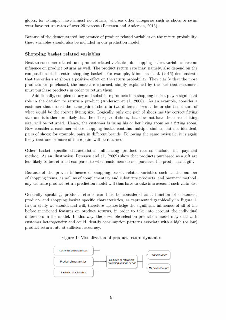
Generally speaking, product returns can thus be considered as a function of customer-,

product- and shopping basket specific characteristics, as represented graphically in Figure 1.

In our study we should, and will, therefore acknowledge the significant influences of all of the

before mentioned features on product returns, in order to take into account the individual

differences in the model. In this way, the ensemble selection prediction model may deal with

customer heterogeneity and could identify consumption patterns associate with a high (or low)

product return rate at sufficient accuracy.

Figure 1: Visualization of product return dynamics

9

In conclusion, although the existing literature presents product return, -behavior and -prediction

in a variety of contexts, it does not incorporate customer-, product- and shopping basket specific

characteristics to its full extent. By focusing on the relation between each of these variables and

product returns, examining the effects of these variables on the return probability, and to use them

to effectively predict product returns, our study will contribute to the existing literature. We

aim to provide a more accurate product return prediction model by examining the behavior and

prediction of these exact measures all together in combination with product returns – something

that has not been done before.

Data Description

Our study uses a database of purchases from a major Dutch online retailer that sells solely

through its online store. Although the online retailer sells products in multiple product

categories, we gather data on purchases within the fashion industry only. The data that is being

used for analysis is cross-sectional taken over the time period from January 2017 until December

2017.

In the past, the return policy of this particular e-commerce retailer encompassed the pos-

sibility for customers to return purchased products within 14 days of purchase, and, if a

customer indeed wished to return one or multiple items, the retailer offered a pick-up service.

However, in November 2017, this policy was changed and the return period of purchased

products was extended to 60 days after purchase.

Additionally, the online retailer limited the payment options of particular return-prone cus-

tomers in September 2017. Knowing that customers who pay after delivery of the ordered prod-

ucts are generally twice as likely to return products in comparison to those who pay in advance

(Urbanke et al., 2015), the online retailer now excludes the option to pay after delivery for partic-

ular return-prone customers in an attempt to reduce the product return rate. This policy change

goes by the name ‘Nudge’ in our study.

The fact that these changes have been made over the period of our dataset may have an

impact on our analysis as different return deadlines, and different payment options may affect

customer’s return decisions differently (Janakiraman and Ordonez, 2012; Urbanke et al., 2015).

In order to control for policy dissimilarities in our sample, we therefore include a dummy variable

that indicates the allowed return deadline at the moment of purchase, and a dummy variable

that indicates the customers who comply with the nudge requirements at the moment of purchase.

The variables that are being used in our analysis are differentiated between three levels,

namely the customer-, product- and shopping basket level. First, the customer level considers

attributes of a particular customer such as a customer’s age, gender, and past return rate;

indicators that are exactly equal for each observation in the basket. Second, the product level

considers indicators such as a product’s brand, price, and color; indicators that may be different

per product in the shopping basket. Third, the shopping basket level of our model captures

features such as the time of purchase, payment method, and the sales channel; indicators that

apply to all products in the shopping basket - however taking into account that some basket

level characteristics (such as the amount of the exact same item) may differ among products in

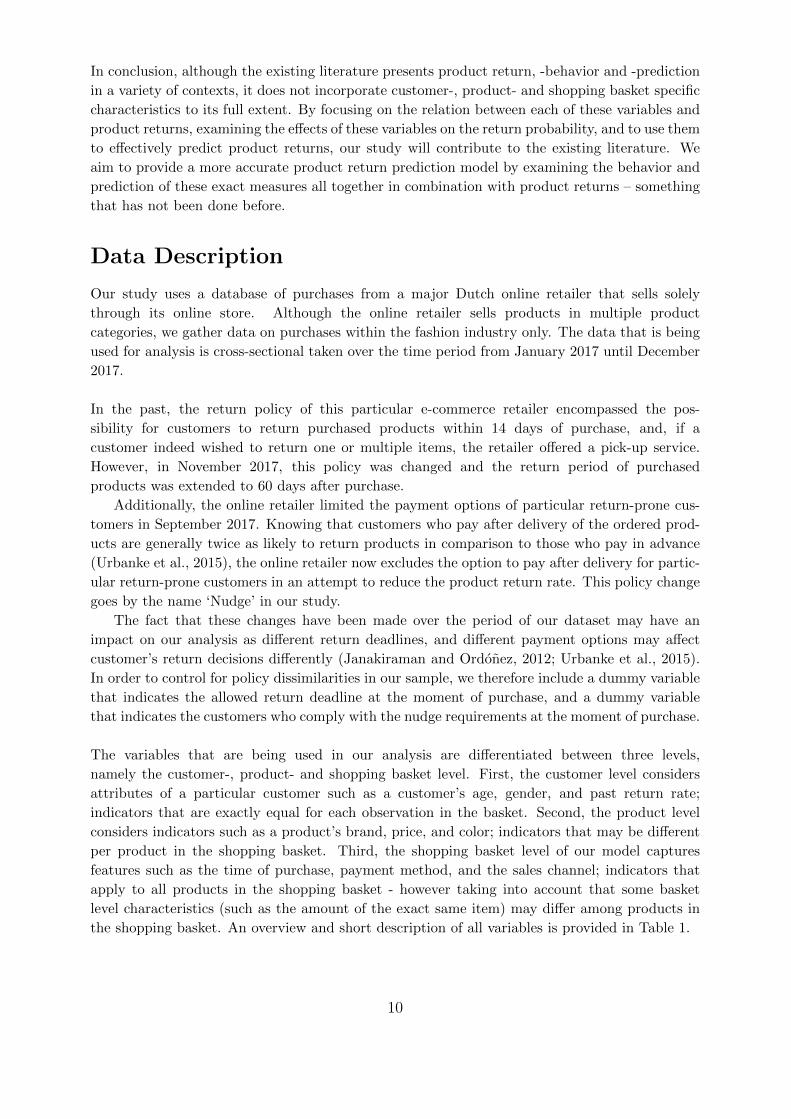
the shopping basket. An overview and short description of all variables is provided in Table 1.

10

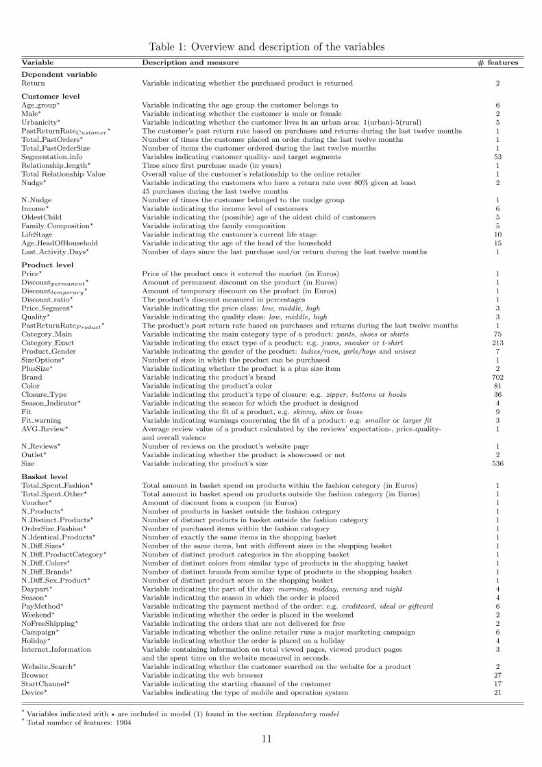
Table 1: Overview and description of the variables

Variable Description and measure # features

Dependent variableReturn Variable indicating whether the purchased product is returned 2

Customer levelAge group? Variable indicating the age group the customer belongs to 6Male? Variable indicating whether the customer is male or female 2Urbanicity? Variable indicating whether the customer lives in an urban area: 1(urban)-5(rural) 5PastReturnRateCustomer

? The customer’s past return rate based on purchases and returns during the last twelve months 1Total PastOrders? Number of times the customer placed an order during the last twelve months 1Total PastOrderSize Number of items the customer ordered during the last twelve months 1Segmentation info Variables indicating customer quality- and target segments 53Relationship length? Time since first purchase made (in years) 1Total Relationship Value Overall value of the customer’s relationship to the online retailer 1Nudge? Variable indicating the customers who have a return rate over 80% given at least 2

45 purchases during the last twelve monthsN Nudge Number of times the customer belonged to the nudge group 1Income? Variable indicating the income level of customers 6OldestChild Variable indicating the (possible) age of the oldest child of customers 5Family Composition? Variable indicating the family composition 5LifeStage Variable indicating the customer’s current life stage 10Age HeadOfHousehold Variable indicating the age of the head of the household 15Last Activity Days? Number of days since the last purchase and/or return during the last twelve months 1

Product levelPrice? Price of the product once it entered the market (in Euros) 1Discountpermanent

? Amount of permanent discount on the product (in Euros) 1Discounttemporary

? Amount of temporary discount on the product (in Euros) 1Discount ratio? The product’s discount measured in percentages 1Price Segment? Variable indicating the price class: low, middle, high 3Quality? Variable indicating the quality class: low, middle, high 3PastReturnRateProduct

? The product’s past return rate based on purchases and returns during the last twelve months 1Category Main Variable indicating the main category type of a product: pants, shoes or shirts 75Category Exact Variable indicating the exact type of a product: e.g. jeans, sneaker or t-shirt 213Product Gender Variable indicating the gender of the product: ladies/men, girls/boys and unisex 7SizeOptions? Number of sizes in which the product can be purchased 1PlusSize? Variable indicating whether the product is a plus size item 2Brand Variable indicating the product’s brand 702Color Variable indicating the product’s color 81Closure Type Variable indicating the product’s type of closure: e.g. zipper, buttons or hooks 36Season Indicator? Variable indicating the season for which the product is designed 4Fit Variable indicating the fit of a product, e.g. skinny, slim or loose 9Fit warning Variable indicating warnings concerning the fit of a product: e.g. smaller or larger fit 3AVG Review? Average review value of a product calculated by the reviews’ expectation-, price quality- 1

and overall valenceN Reviews? Number of reviews on the product’s website page 1Outlet? Variable indicating whether the product is showcased or not 2Size Variable indicating the product’s size 536

Basket levelTotal Spent Fashion? Total amount in basket spend on products within the fashion category (in Euros) 1Total Spent Other? Total amount in basket spend on products outside the fashion category (in Euros) 1Voucher? Amount of discount from a coupon (in Euros) 1N Products? Number of products in basket outside the fashion category 1N Distinct Products? Number of distinct products in basket outside the fashion category 1OrderSize Fashion? Number of purchased items within the fashion category 1N Identical Products? Number of exactly the same items in the shopping basket 1N Diff Sizes? Number of the same items, but with different sizes in the shopping basket 1N Diff ProductCategory? Number of distinct product categories in the shopping basket 1N Diff Colors? Number of distinct colors from similar type of products in the shopping basket 1N Diff Brands? Number of distinct brands from similar type of products in the shopping basket 1N Diff Sex Product? Number of distinct product sexes in the shopping basket 1Daypart? Variable indicating the part of the day: morning, midday, evening and night 4Season? Variable indicating the season in which the order is placed 4PayMethod? Variable indicating the payment method of the order: e.g. creditcard, ideal or giftcard 6Weekend? Variable indicating whether the order is placed in the weekend 2NoFreeShipping? Variable indicating the orders that are not delivered for free 2Campaign? Variable indicating whether the online retailer runs a major marketing campaign 6Holiday? Variable indicating whether the order is placed on a holiday 4Internet Information Variable containing information on total viewed pages, viewed product pages 3

and the spent time on the website measured in seconds.Website Search? Variable indicating whether the customer searched on the website for a product 2Browser Variable indicating the web browser 27StartChannel? Variable indicating the starting channel of the customer 17Device? Variables indicating the type of mobile and operation system 21

* Variables indicated with ? are included in model (1) found in the section Explanatory model* Total number of features: 1904

11

Most of the variables in Table 1 are self-explanatory and do not need to be elaborated on any

further. However, in light of the complexity of some, we provide additional explanation for those

variables that we see fit.

A variable that we think does require further explanation, is the product’s past return

rate, for instance. In order to calculate this, we consider historical purchase and return data

from twelve months prior to the actual purchase. However, it may be possible that the sample

size of the historic product data is small, which could result in an inconsistent and biased

calculation of the past return rate. These small sample sizes are usually observed when a

product is new on the market or when a product has a small stock. In such cases, the product’s

past return rate is estimated by taking the average of the past return rates from similar type of

products that fall within the same quality- and price segment.

Furthermore, the quality segment of products is determined by the product’s price at the

moment it entered the market for the reason that, as explained in the literature review of this

study, the product’s price may capture the product’s quality (Kirmani and Rao, 2000; Monroe,

1973). In more detail, for each product type category, the deciles are calculated using the

price of the product at the moment it entered the market, and all other introduction prices of

products that are on the market at this particular moment. The products that then fall in the

first three deciles correspond to a low quality product, whereas high quality products are within

the last three deciles. The products that fall between the first- and last three deciles are defined

as medium quality products.

The price segments are calculated the way the quality segments of products are determined.

However, now the deciles are based on the product’s price at the moment of purchase instead of

the product’s price at the moment of entering the online shop.

Lastly, the total relationship value is calculated in a manner demonstrated before by

Griffis et al. (2012). In simple terms, the total relationship value equals the total expenditure of

a customer during the last twelve months. For customer i, it is calculated by TRVi = Fi×Ni×Vi,where Fi denotes the customer’s order frequency during the last 12 months, Ni the customer’s

average number of ordered products during the last 12 month, and Vi the customer’s average

product value during the last 12 months.

In our study we are exclusively interested in estimating returns. Therefore, we exclude

other outcomes such as denied-, undelivered- or canceled orders. The sample, after deletion

of observations which do not satisfy the requirement stated previously, consist of 16,750,953

purchases from 4,818,306 orders of 1,343,654 unique customers. The data is related to sales of

over 150,410 distinct fashion items, which were either returned or kept by the customer. The

average return rate over the year 2017 was 52.77 percent.

Customers purchase on average 4 products within an order where the average price of a

product is about e37. Furthermore, the average age of the customers in the sample is 42 years,

whereas 78 percent of the respondents is female. The majority of the population, that is, 57

percent, are families and respectively, 22 and 25 percent of the respondents has a modal income

or an income that is 1.5× higher than the modal income.

More summary statistics are provided in Table 2 below. Because some events rarely occur,

12

we only present the attribute levels that appear the most.

Table 2: Descriptive statistics

Statistic N Mean St. Dev. Min Max

Return 16,750,953 0.5277 0.4992 0 1Price 16,750,953 37.13 28.54 1.00 1789.00Total OrderSize 4,818,306 3.735 3.602 1 57Male 1,343,654 0.2210 0.4148 0 1Age 4,642,509 42.29 11.88 0 118IncomeModal 1,343,654 0.2238 0.4168 0 1Income1.5×Modal 1,343,654 0.2587 0.4379 0 1Family CompostionFamilies 1,343,654 0.5716 0.4948 0 1Family CompostionSingles 1,343,654 0.1731 0.3783 0 1Family CompostionOlderCouples 1,343,654 0.1636 0.3699 0 1Relationship length 4,642,509 7.22 4.51 0 21.41Total PastOrders 4,818,306 10.60 16.78 0 663Total PastOrdersize 4,818,306 40.59 66.33 0 1853Total PastReturns 4,818,306 22.734 49.186 0 1390LastPurchase Days 4,818,306 49.27 70.57 0 367LastReturn Days 4,818,306 46.85 74.53 0 367Nudge 4,818,306 0.057 0.231 0 1Total Spent Fashion 4,818,306 129.10 140.71 1.00 4149.30Total Spent Other 4,818,306 9.53 43.90 0 4738.19Website Search 4,818,306 0.234 0.423 0 1StartChannelDirectLoad 4,818,306 0.3308 0.4705 0 1StartChannelSEA Branded 4,818,306 0.1917 0.3936 0 1StartChannelSEA Non Branded 4,818,306 0.1539 0.3609 0 1DeviceDesktop 4,818,306 0.4431 0.4967 0 1DeviceMobile 4,818,306 0.3601 0.4800 0 1DeviceTablet 4,818,306 0.1863 0.3893 0 1

* Note that for all dummy variables, the value of 1 denotes the occurrence is true. The lastpurchase- and return days have a maximum of 367 which indicates that the customer placedan order more than 365 days ago.

As can be seen in Table 2, there seem to be some outliers and missing observations in the data.

For example, the variable Age has 4,642,509 observations and a range from 0 to 118. This suggest

that the true age of a customer is missing, or not observed in some cases. Nonetheless, outliers are

not omitted from the data as dealing with such outliers is a practical issue that is rather common

for online retailers. As the focus of this study is to provide an accurate- , but also realistic- and

practical model as possible, it is especially important that we include such practical issues in our

model as well. To explain the effects of the independent variables on product returns, however,

both the outliers as well as missing observations are omitted from our study as they may cause

inconsistent and biased results.

Methodology

To inspect the data further, we construct multiple models including an explanatory model

and multiple predictive models. The first of these, the explanatory model, attends to explain

phenomena at a conceptual level. In this sense, the explanatory model is used to provide insights

in the dynamics of factors that may influence a consumer’s decision to return a product; insights

in the influence of customer-, product-, and shopping basket characteristics on a customer’s

return behavior, for example. The latter, the predictive models, tend to be used to produce

expectations of future behavior that are measurable; concrete estimations of the likelihood

of a product return. Although there exist diverse statistical methods that are able to both

13

explain- and predict a certain outcome, in our study, the predictive models are exclusively used

to estimate this concrete likelihood of a product return, while the explanatory model provides

further insights as to what causes this likelihood estimation. Both types of models can be of

particular use in providing online retailers with critical information to base their product return

strategies on.

During this study all of the statistical analyses are conducted using R for Windows (R

Core Team, 2015).

Explanatory model

To analyze the drivers of product returns binomial logistic regressions are applied as statistical

method, since it allows prediction of a binary dependent variable based on the analysis of the

independent variables. Recall that in this study the dependent variable of interest is Return,

which is a dummy variable. Logistic regression seems appropriate as previous studies have

applied this technique in examining the influence of various factors on the return probability

(Hess and Mayhew, 1997; Minnema et al., 2016).

As stated in the literature review, product returns can be considered as a function of

customer-, product-, and shopping basket specific variables. However, other factors, such as

situation specific factors like major marketing campaigns or seasonal patterns, may influence

return decision as well. In order to control for customer variation, and heterogeneity, we

therefore include these situation specific factors as control variables. Accordingly, the probability

that customer i returns product j bought at day t can be expressed as,

P(Returnijt = 1|Xijt, εijt

)=

1

1 + e−Xijtβ, where (1)

Xijtβ =β1Customer Levelit + β2Product Leveljt + β3Basket Levelijt

+ β4Control V ariablesijt + β0 + εijt,

and Customer Levelit denotes the vector of customer related variables, Product Leveljt is the

vector of product related variables, Basket Levelijt is the vector of shopping basket related

variables, and Control V ariablesijt denotes the vector of control related variables. The exact

variables contained in these four vectors are given in Table 1 as indicated by a star (?). Then,

β1−4 denote the vector of parameters (i.e., effects) for the different sets of variables, β0 represent

the intercept and εijt is the unobserved individual error term.

When estimating the model parameters we might encounter ‘the p-value problem’, namely, due

to large-sample issues, relying solely on the p-value and coefficient signs is ill-advised, because

p-values approach zero for large samples (Lin et al., 2013). Contrarily, relying on a Confidence

Interval (CI) is always safe, because the CI will become narrower as the sample size increases.

While the information that CIs convey thus does scale up to large samples, as the range

estimate becomes more precise, the information contained in p-values does not. We therefore

also calculate 95% CIs for the estimated coefficients.

In our research, we estimate model (1) in steps, in order to examine possible changes in the

coefficients. In this way we investigate whether the addition of variables has a large influence on

14

the significance and altitude of the coefficients.

Moreover, with each step we use the Likelihood Ratio Test (LRT) to test whether the

additional variables yield additional explanatory value and are indeed more appropriate to use.

Besides the LRT, the Akaike Information Criterion (AIC) provides a method for assessing

the quality of the model through comparison of related models introduced by Akaike (1974).

The AIC is based on the deviance, but includes a penalty for overfitting. In other words, the

AIC rewards goodness of fit, though intent to prevent including irrelevant variables in the model.

So is the Bayesian Information Criteria (BIC), which is similar to the AIC, but with a larger

penalty term (Schwarz et al., 1978). Although the AIC and BIC itself are not interpretable, they

are useful for comparing models. For more than one similar candidate model (where all of the

variables of the simpler model occur in the more complex models), the model which corresponds

with the smallest AIC and BIC should be selected.

In the first step, only the demographic customer variables are included, in order to define

their effects on the probability of a product return. Note that we explained in the literature

review the correlation of these demographic variables to product returns. In the second step we

include the product specific variables, to control for product differences in the sample, whereas

in the third step we include the shopping basket characteristics as well. At last, we include the

control variables to take into account seasonality, marketing campaigns and return policy effects.

Before we interpret the results of our final model we test for multicollinearity using the

Variance Inflation Factors (VIF). The VIF provides an index that measures how much the

variance of an estimated regression coefficient is increased due to collinearity. The VIF factor

for the ith regression coefficient βi is calculated by,

VIFi =1

1−R2i

,

where R2i is the coefficient of determination of the regression in which the ith independent

variable is predicted by all the other independent variables. Higher levels of VIF reveal

multicollinearity, but Craney and Surles (2002) point out that there is no general cutoff value

for the VIF. However, a value of 10 as the maximum level of VIF is common (Kutner et al., 2004).

Finally, to explain how return decisions are influenced by customer-, product-, and shop-

ping basket characteristics, we calculate marginal effects. Marginal effects measure the

instantaneous effect that a change in a particular explanatory variable has on the predicted

probability of the dependent variable, when all other covariates are kept fixed. Thus, in our

context, they can measure how a change in a covariate is related to the return probability. For

our final model, the marginal effect of covariate k is given by,

Marginal Effect xk =∂P(Returnijt = 1|Xijt, εijt

)∂xk

=eXijtβ

1 + eXijtβ

∂Xijtβ

xk= P

(Returnijt = 1|Xijt, εijt

)× P

(Returnijt = 0|Xijt, εijt

)× βk.

This expression shows that the marginal effect depends not only on βk, but on the value of all

variables in Xijt. Hence, in order to calculate the exact impact of covariate k on the return

probability, values for Xijt are necessary. To this extent, it is common to set all variables to their

15

means, which is also known as the Average Marginal Effect (AME). To assess the magnitude of

an effect for our explanatory variables, we therefore calculate the AME of each covariate in our

final model.

The standard errors of the AMEs are computed using the Delta-Method, but for the fear

that the AMEs are not normally distributed, we also calculate bootstrapped standard errors

and compare the results.

The data we use to analyze the drivers of product returns consist of 600,000 observations

of customer purchases coming from a random subset of the original data.

Predictive models

The success of ensemble modeling relies on the diversity of candidate models (Kuncheva, 2004).

In our study we select a total of eight different candidate models that have been shown to be

effective prediction models, namely Adaptive Boosting (Adaboost), Extreme Gradient Boosting

(EGB), k Nearest Neighbors (KNN), logistic regression (Logit), Multilayer Perceptron (MLP),

Naive Bayes (NB), Non-Linear Support Vector Machine (SVM), and the Random Forest (RF)

(Partalas et al., 2010; Fernandez-Delgado et al., 2014; Urbanke et al., 2015; Heilig et al., 2016).

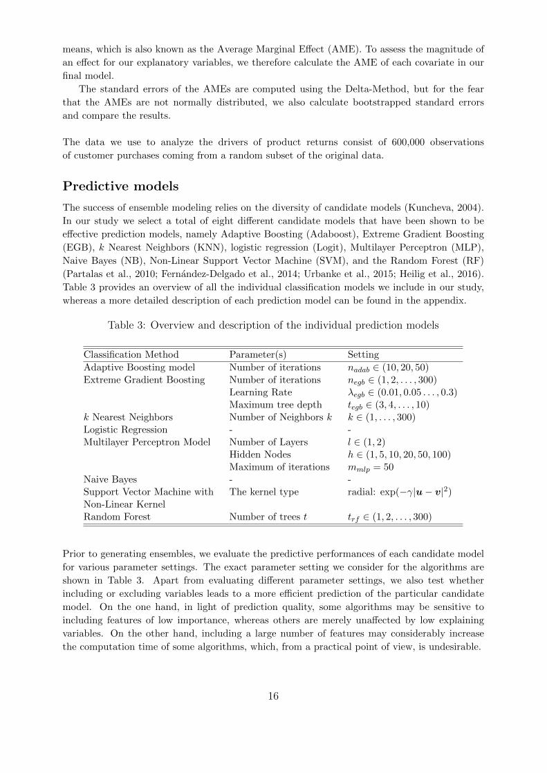
Table 3 provides an overview of all the individual classification models we include in our study,

whereas a more detailed description of each prediction model can be found in the appendix.

Table 3: Overview and description of the individual prediction models

Classification Method Parameter(s) Setting

Adaptive Boosting model Number of iterations nadab ∈ (10, 20, 50)Extreme Gradient Boosting Number of iterations negb ∈ (1, 2, . . . , 300)

Learning Rate λegb ∈ (0.01, 0.05 . . . , 0.3)Maximum tree depth tegb ∈ (3, 4, . . . , 10)

k Nearest Neighbors Number of Neighbors k k ∈ (1, . . . , 300)Logistic Regression - -Multilayer Perceptron Model Number of Layers l ∈ (1, 2)

Hidden Nodes h ∈ (1, 5, 10, 20, 50, 100)Maximum of iterations mmlp = 50

Naive Bayes - -Support Vector Machine with The kernel type radial: exp(−γ|u− v|2)Non-Linear KernelRandom Forest Number of trees t trf ∈ (1, 2, . . . , 300)

Prior to generating ensembles, we evaluate the predictive performances of each candidate model

for various parameter settings. The exact parameter setting we consider for the algorithms are

shown in Table 3. Apart from evaluating different parameter settings, we also test whether

including or excluding variables leads to a more efficient prediction of the particular candidate

model. On the one hand, in light of prediction quality, some algorithms may be sensitive to

including features of low importance, whereas others are merely unaffected by low explaining

variables. On the other hand, including a large number of features may considerably increase

the computation time of some algorithms, which, from a practical point of view, is undesirable.

16

After tuning each candidate model we then start to generate ensembles. There are many ap-

proaches to construct an ensemble. These include the various ways in which the predictions of

the candidate models may be combined. To this extent, the most basic and convenient way is a

simple averaging. With averaging, the predictions of each candidate model are equally weighted

and the ensemble calculates the average prediction.

A more advanced technique to combine information from multiple predictive models is

known as stacking. With stacking, a combiner algorithm is used to put together the output from

the candidate models, where in practice, a logistic regression model is often used as the combiner

algorithm. Hence, a stacked ensemble trains all of the candidate models using the available data

first, then a combiner algorithm is fitted to make a final prediction using all the predictions of

the candidate models as inputs. In many instances, stacking outperforms each of the individual

classification models due to its smoothing nature and ability to highlight each base model where

it performs best and discredit each candidate model where it performs poorly.

In summary, concerning the prediction of product returns, in our analysis we consider a

total of eight candidate models when creating ensembles through averaging and stacking, with

logistic regression as the combiner algorithm. The total number of unique ensembles (m) one

could generate from n individual models is then given by m = 2 ×(2n − (n + 1)

), which

exponentially increases as n increases. Hence, our eight candidate models result in 494 unique

averaging- and stacking ensembles to consider.

Although our study constructs and evaluates all 494 unique averaging- and stacking en-

sembles, we ultimately discusses only six out of these, namely, two ensembles (using averaging

and stacking) that consider all eight candidate models; two ensembles (using averaging and

stacking) corresponding to the best composition of candidate models which have the best

average predictive quality based on averaging, and lastly; two ensembles (using averaging and

stacking) corresponding to the best composition of candidate models which have the best average

predictive quality found by stacked generalization.

Validation measures

To asses the performance of our prediction models, we follow the procedure of model validation

given in Vergouwe (2003), which distinguishes several aspects of validity, namely overall perfor-

mance, calibration, discrimination and practical usefulness. The overall performance captures

both calibration and discrimination aspects. To this end, calibration concerns the agreement

between observed probabilities and predicted probabilities, and procedures in statistical classifi-

cation to determine class membership of a given new observation. Discrimination concerns the

ability of the prediction model to properly distinguish between subjects with different outcomes.

Hence, in our context, discrimination measures how well the model can distinguish between

purchases that do return and those that are kept. Finally, the ability of the prediction model to

improve the decision making process is captured by the practical usefulness.

The model validation measures are calculated for all single classifiers, ensemble learners,

and the proposed ensembles. In this way the performances of all prediction models incorporated

in our study are investigated which enables us to answer our sub-question.

17

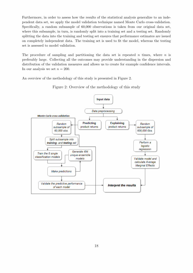
Furthermore, in order to assess how the results of the statistical analysis generalize to an inde-

pendent data set, we apply the model validation technique named Monte Carlo cross-validation.

Specifically, a random subsample of 60,000 observations is taken from our original data set,

where this subsample, in turn, is randomly split into a training set and a testing set. Randomly

splitting the data into the training and testing set ensures that performance estimates are issued

on completely independent data. The training set is used to fit the model, whereas the testing

set is assessed to model validation.

The procedure of sampling and partitioning the data set is repeated n times, where n is

preferably large. Collecting all the outcomes may provide understanding in the dispersion and

distribution of the validation measures and allows us to create for example confidence intervals.

In our analysis we set n = 200.

An overview of the methodology of this study is presented in Figure 2.

Figure 2: Overview of the methodology of this study

18

Overall performance

Regarding the overall performance of our prediction models, the predictive accuracy and the

Area Under the ROC-curve (AUC) are used as validation measures.

The predictive accuracy could be used as a statistical measure of how many observations

in the testing set are correctly classified. It is calculated from predicted probabilities, where in

our case the predicted probability denotes the probability of a purchased product being fitted

with a return; mathematically denoted by P (Returnijt = 1|Xijt), where Xijt contains the

independent variables. However, in order to practically assign the corresponding class to the

predicted probability of each purchased product, a decision boundary is needed.

For instance, by setting the decision boundary equal to the traditional default of 0.5, we

conclude that the dummy variable Returnijt = 1 if P (Returnijt = 1|Xijt) > 0.5 and otherwise

Returnijt = 0. This threshold is of great importance, because it ultimately decides the predicted

class of observations and could therefore have a dramatic impact on the model’s quality in terms

of predictive accuracy.

There exist numerous possibilities to determine the optimal threshold value (Liu et al.,

2005; Freeman and Moisen, 2008). These include subjective approaches such as taking a

fixed value like the traditional default of 0.5, or a threshold that meets a given management

requirement. More objective approaches are based on the dataset where the threshold is set to,

for example, the mean probability of occurrence of the dependent variable. Objective approaches

typically select the threshold that maximizes the agreement between observed and predicted

classes. To this extent, one could determine the optimal cut-off point using the Receiver

Operating Characteristic curve (ROC-curve).

The ROC graph provides a method of evaluating the performance of prediction models.

It is created by plotting the true positive rate (sensitivity) against the false positive rate

(1-specificity) for a threshold value which varies from 0 to 1. At the diagonal, the true positive

rate equals the false positive rate which implies that the model makes random predictions. Ideal

models realize a high true positive rate, whereas the false positive rate remains small. The

ROC-curve of a well-defined model thus rises steeply close to the origin and flattens at a value

near the maximum of 1. On the contrary, the ROC-curve of a poor model lies adjacent to the

diagonal, because at the diagonal the true positive rate equals the false positive rate which

implies, as previously mentioned, that the model makes random predictions.

Since the upper left corner of the ROC plot can be considered as the ‘perfect’ model,

the threshold which minimizes the distance between the ROC-curve and this ‘perfect’ point is

appropriate to use as an optimal cut-off point. In truth, it is shown that selecting the threshold

based on the shortest distance to the top-left corner in ROC plot is indeed a good method to

find the optimal cut-off (Liu et al., 2005; Freeman and Moisen, 2008; Kumar and Indrayan, 2011).

In our analysis we therefore use this method to provide us with the threshold which is

used to classify the predicted probabilities into a class. Comparison of the predicted classes and

the observed classes then yields the predictive accuracy for the model, calculated by taking the

mean of correctly predicted observations.

19

In some instances, however, the results of the predictive accuracy must be approached

with caution, as the predictive accuracy could only reflect the underlying class distribution.

In other words, a disproportionately high number of members from one class could result in a

classifier that is biased to this class. For example, suppose that 80% of the fashion products are

returned, then a constant prediction of a product return is bound to be correct 80% of the time,

although this predictive accuracy is truly non-informative and useless. This problem is known

as the accuracy paradox, but as Table 2 reveals a mean return rate of 52.77%, the accuracy

paradox does not appear to be a problem in our case.

In light of the ROC-curve, it follows that the area under the ROC-curve (AUC) is a

well-defined measure for overall model performance, in particular for discrimination ability

(Steyerberg et al., 2010). From this perspective, ideal models have an AUC approximating 1,

while random models have an AUC of 0.5.

Calibration and discrimination

Accurate prediction models discriminate between those with and those without the outcome.

Ideally, for a prediction model to excellently distinguish between observations with different

outcomes, the predicted probabilities approximate 1 for the respondents with the outcome,

whereas the predicted probabilities are close to 0 for those without the outcome. To this

extent, a wide spread in the distribution of the predicted probabilities (away from the average

probability) is evidence in favor for a good discriminating model.

To visualize the discriminative ability of our prediction models we therefore create his-

tograms that plot the distribution of the predicted probabilities, conditional on the observed

outcome.

The interpretation of this histogram is as follows: on the basis of the testing set, for a

given predicted probability value on the x-axis, one can find the total number of times this

particular predicted probability value is observed, conditional on the true observed class, against

the y-axis. Perfect discriminating models show no overlap in the predicted probability values of

each observed class, whereas the predicted probability values of classes completely overlap for a

random models. Roughly, the less overlap the graph shows, the better the model is able to dis-

criminate between the classes, and the more accurate the model is able to predict product returns.

Well calibrated prediction models are probabilistic models for which the output can be

directly interpreted as a confidence level. A well calibrated prediction model, for example,

should classify the samples such that among the samples to which it gave a predicted probability

value close to 0.8 for belonging to a particular class, approximately 80% actually belong to that

class. Hence, the histograms that help to visualize the discriminative ability of our prediction

models, can also help to provide additional insights in the calibration. Especially, biases in the

predicted probabilities may be observed.

20

Practical usefulness

As mentioned before, an accurate prediction of a customer’s likelihood to return a product

could constitute a contribution to many online retailers’ overall profit margins. That is to

say because it is essential to account for product returns when calculating CLV (Minnema

et al., 2018), but product return predictions could also facilitate online retailers with a number

of return preventive actions, such as the aforementioned moral suasion. Other examples of

preventive actions are to offer a coupon conditioned by the fact that the product is not returned

to customers who display a high risk of returning, or more invasive, to charge a risk premium

through increasing the product price.

Recognizing that product returns are inherently part of online retailers’ business model,

systems for prediction and prevention of product returns should only focus on extreme cases. In

our case, the extreme cases are defined as the purchases that are expected to be most likely to

be returned.

In order to evaluate the impact that our prediction models could have on the online re-

tailer’s profits, we are then particularly interested in two aspects. First, how many out of all

the purchases we expect to be returned, are actually returned, and second, how many out of all

the purchases that are actually returned, were identified as a product return by our prediction

models. These aspects are also known as precision and recall, and are calculated by,

Precision =TP

TP + FPand Recall =

TP

TP + FN, (2)

where TP denotes the true positives, FP the false positives, and FN the false negatives.

As last validation measures we therefore calculate precision and recall, while focusing

solely on product purchases with a very high return probability. It is important to keep in mind,

however, that there is a trade-off between these measures. That is to say because expecting

more product returns will increase the precision, but will reduce the recall.

Results

Explaining product returns

Binominal logistic regression models are performed for the dependent variable Return to inspect

the data for the drivers of product returns. The logistic regression models where the variables

are added stepwise are given in Table A.2, presented in the appendix.

This table reveals that, all in all, the coefficients of the independent variables do not

vary significantly for any of the models, although, with some exceptions. For instance, one can

observe that the coefficient of Age25to34 becomes significant once the product level variables are

included, and then reverses in the third column as we include shopping basket characteristics,

while the results for all other age groups are roughly constant over the steps. Note that the

reference level of the age groups are customers under the age of 24. This suggest that, especially

between this group of customers and customers aged between 25 and 34, the return behavior

significantly varies, when adjusting for product- and shopping basket characteristics.

21

Another example of a varying coefficient concerns the variable Discounttemporary, which

becomes insignificant once the shopping basket variables are included. This implies that

Discounttemporary and the shopping basket variables explain the same effect on the return

probability, which results the coefficient of Discounttemporary to become insignificant.

Generally, the reason of possible changes in the coefficients is that the addition of variables

in a model likely changes the bivariate relationship between a independent variable, the other

independent variables and the dependent variable. This provides an explanation of sign reversals

or varying significancy of coefficients one may observe in Table A.2.

As described in the methodology, several measures are taken in order to evaluate the final model.

In each step, LRT tests are performed followed by comparison of both AIC and BIC. Table A.1

in the appendix reports the exact results of the LRT, whereas the AIC and BIC can be found in

Table A.2. Certainly, the LRTs indicate that the inclusion of extra variables (e.g., product- and

basket characteristics) yield more explanatory value for all models. The AIC and BIC support

this finding by showing that the AIC and BIC are the lowest for the final model. This also

suggest that for the prediction of product returns it is desirable to use customer-, product-, and

basket characteristics. At last, multicollinearity does not appear to be a concern in our analy-

sis as none of the variables in the stepwise models show a VIF which exceeds the threshold of 10.

Table 4 shows our final model that is used to analyze the drivers of returns, where the

average marginal effects of the logistic regression from our final model is provided. The average

marginal effects can be interpreted as follows: for a change in one of the independent variables,

the corresponding estimated coefficient represents the average change in the probability to return

a product within the fashion category, ceteris paribus.

Additionally, we present the CIs associated with the average marginal effects, which are based

on standard errors computed by the delta-method2. Recall that we determine the CIs because

we were likely to be misguided by p-values due to the large sample size. However, the results do

not support our suspicion of the p-value problem. That is to say because not all independent

variables are highly significant (while believing that not each effect of the covariates on the return

probability is truly zero), indicating that the sample size is not large enough to let all p-values

approach to zero.

2Bootstrapped standard errors (1000 samples) gave similar results.

22

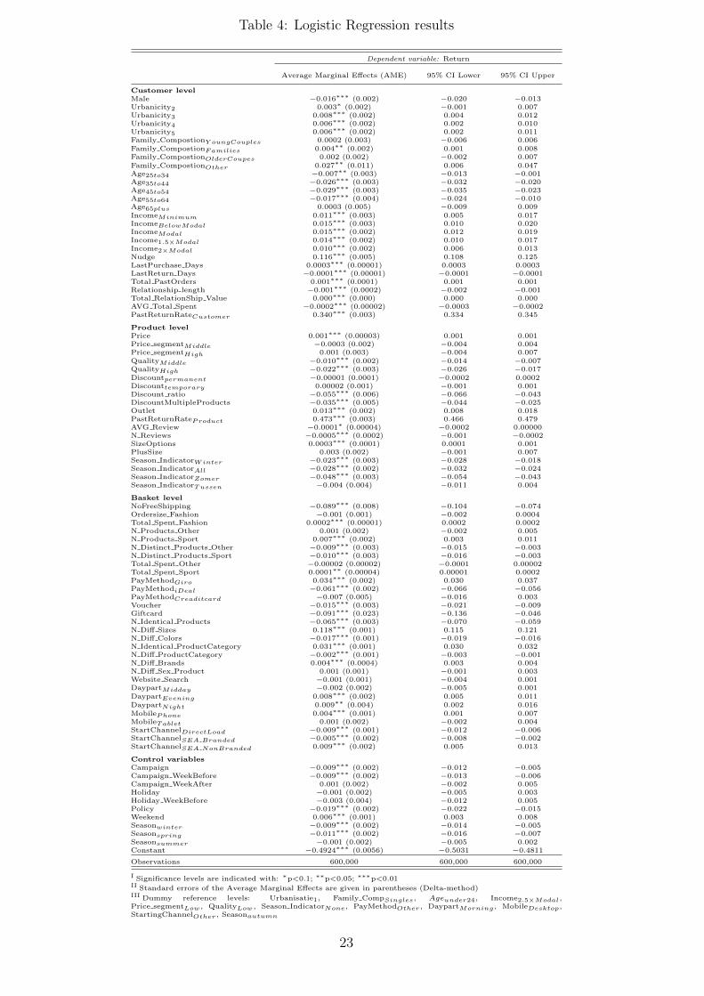
Table 4: Logistic Regression results

Dependent variable: Return

Average Marginal Effects (AME) 95% CI Lower 95% CI Upper

Customer levelMale −0.016∗∗∗ (0.002) −0.020 −0.013Urbanicity2 0.003∗ (0.002) −0.001 0.007Urbanicity3 0.008∗∗∗ (0.002) 0.004 0.012Urbanicity4 0.006∗∗∗ (0.002) 0.002 0.010Urbanicity5 0.006∗∗∗ (0.002) 0.002 0.011Family CompostionY oungCouples 0.0002 (0.003) −0.006 0.006Family CompostionFamilies 0.004∗∗ (0.002) 0.001 0.008Family CompostionOlderCoupes 0.002 (0.002) −0.002 0.007Family CompostionOther 0.027∗∗ (0.011) 0.006 0.047Age25to34 −0.007∗∗ (0.003) −0.013 −0.001Age35to44 −0.026∗∗∗ (0.003) −0.032 −0.020Age45to54 −0.029∗∗∗ (0.003) −0.035 −0.023Age55to64 −0.017∗∗∗ (0.004) −0.024 −0.010Age65plus 0.0003 (0.005) −0.009 0.009IncomeMinimum 0.011∗∗∗ (0.003) 0.005 0.017IncomeBelowModal 0.015∗∗∗ (0.003) 0.010 0.020IncomeModal 0.015∗∗∗ (0.002) 0.012 0.019Income1.5×Modal 0.014∗∗∗ (0.002) 0.010 0.017Income2×Modal 0.010∗∗∗ (0.002) 0.006 0.013Nudge 0.116∗∗∗ (0.005) 0.108 0.125LastPurchase Days 0.0003∗∗∗ (0.00001) 0.0003 0.0003LastReturn Days −0.0001∗∗∗ (0.00001) −0.0001 −0.0001Total PastOrders 0.001∗∗∗ (0.0001) 0.001 0.001Relationship length −0.001∗∗∗ (0.0002) −0.002 −0.001Total RelationShip Value 0.000∗∗∗ (0.000) 0.000 0.000AVG Total Spent −0.0002∗∗∗ (0.00002) −0.0003 −0.0002PastReturnRateCustomer 0.340∗∗∗ (0.003) 0.334 0.345

Product levelPrice 0.001∗∗∗ (0.00003) 0.001 0.001Price segmentMiddle −0.0003 (0.002) −0.004 0.004Price segmentHigh 0.001 (0.003) −0.004 0.007QualityMiddle −0.010∗∗∗ (0.002) −0.014 −0.007QualityHigh −0.022∗∗∗ (0.003) −0.026 −0.017Discountpermanent −0.00001 (0.0001) −0.0002 0.0002Discounttemporary 0.00002 (0.001) −0.001 0.001Discount ratio −0.055∗∗∗ (0.006) −0.066 −0.043DiscountMultipleProducts −0.035∗∗∗ (0.005) −0.044 −0.025Outlet 0.013∗∗∗ (0.002) 0.008 0.018PastReturnRateProduct 0.473∗∗∗ (0.003) 0.466 0.479AVG Review −0.0001∗ (0.00004) −0.0002 0.00000N Reviews −0.0005∗∗∗ (0.0002) −0.001 −0.0002SizeOptions 0.0003∗∗∗ (0.0001) 0.0001 0.001PlusSize 0.003 (0.002) −0.001 0.007Season IndicatorWinter −0.023∗∗∗ (0.003) −0.028 −0.018Season IndicatorAll −0.028∗∗∗ (0.002) −0.032 −0.024Season IndicatorZomer −0.048∗∗∗ (0.003) −0.054 −0.043Season IndicatorTussen −0.004 (0.004) −0.011 0.004

Basket levelNoFreeShipping −0.089∗∗∗ (0.008) −0.104 −0.074Ordersize Fashion −0.001 (0.001) −0.002 0.0004Total Spent Fashion 0.0002∗∗∗ (0.00001) 0.0002 0.0002N Products Other 0.001 (0.002) −0.002 0.005N Products Sport 0.007∗∗∗ (0.002) 0.003 0.011N Distinct Products Other −0.009∗∗∗ (0.003) −0.015 −0.003N Distinct Products Sport −0.010∗∗∗ (0.003) −0.016 −0.003Total Spent Other −0.00002 (0.00002) −0.0001 0.00002Total Spent Sport 0.0001∗∗ (0.00004) 0.00001 0.0002PayMethodGiro 0.034∗∗∗ (0.002) 0.030 0.037PayMethodiDeal −0.061∗∗∗ (0.002) −0.066 −0.056PayMethodCreaditcard −0.007 (0.005) −0.016 0.003Voucher −0.015∗∗∗ (0.003) −0.021 −0.009Giftcard −0.091∗∗∗ (0.023) −0.136 −0.046N Identical Products −0.065∗∗∗ (0.003) −0.070 −0.059N Diff Sizes 0.118∗∗∗ (0.001) 0.115 0.121N Diff Colors −0.017∗∗∗ (0.001) −0.019 −0.016N Identical ProductCategory 0.031∗∗∗ (0.001) 0.030 0.032N Diff ProductCategory −0.002∗∗∗ (0.001) −0.003 −0.001N Diff Brands 0.004∗∗∗ (0.0004) 0.003 0.004N Diff Sex Product 0.001 (0.001) −0.001 0.003Website Search −0.001 (0.001) −0.004 0.001DaypartMidday −0.002 (0.002) −0.005 0.001DaypartEvening 0.008∗∗∗ (0.002) 0.005 0.011DaypartNight 0.009∗∗ (0.004) 0.002 0.016MobilePhone 0.004∗∗∗ (0.001) 0.001 0.007MobileTablet 0.001 (0.002) −0.002 0.004StartChannelDirectLoad −0.009∗∗∗ (0.001) −0.012 −0.006StartChannelSEA Branded −0.005∗∗∗ (0.002) −0.008 −0.002StartChannelSEA NonBranded 0.009∗∗∗ (0.002) 0.005 0.013

Control variablesCampaign −0.009∗∗∗ (0.002) −0.012 −0.005Campaign WeekBefore −0.009∗∗∗ (0.002) −0.013 −0.006Campaign WeekAfter 0.001 (0.002) −0.002 0.005Holiday −0.001 (0.002) −0.005 0.003Holiday WeekBefore −0.003 (0.004) −0.012 0.005Policy −0.019∗∗∗ (0.002) −0.022 −0.015Weekend 0.006∗∗∗ (0.001) 0.003 0.008Seasonwinter −0.009∗∗∗ (0.002) −0.014 −0.005Seasonspring −0.011∗∗∗ (0.002) −0.016 −0.007Seasonsummer −0.001 (0.002) −0.005 0.002Constant −0.4924∗∗∗ (0.0056) −0.5031 −0.4811

Observations 600,000 600,000 600,000

I Significance levels are indicated with: ∗p<0.1; ∗∗p<0.05; ∗∗∗p<0.01II Standard errors of the Average Marginal Effects are given in parentheses (Delta-method)III Dummy reference levels: Urbanisatie1, Family CompSingles, Ageunder24, Income2.5×Modal,Price segmentLow , QualityLow , Season IndicatorNone, PayMethodOther , DaypartMorning , MobileDesktop,StartingChannelOther , Seasonautumn

23

Customer characteristics

The logistic regression results on the dependent variable Return in Table 4 show several sig-

nificant effects of customer demographics on the return probability. The results present, for

example, a negative effect of Male (AME Male =-0.016) on the probability of a product return

at the 1% significant level. Hence, granted that a customer is a man, the probability of a product

return decreases by 1.6% on average, ceteris paribus. More informative is the 95% CI which

exposes that being a male customer decreases the probability of a return on average between

1.3% and 2%, with 95% confidence. Regarding the living area of a customer, the customers who

live in more rural areas have a higher average return probability in comparison to the customers

who live in urban areas. Both these findings support the study of Minnema et al. (2016).

Other customer demographics, however, exert also significant effects on the return prob-

ability. For example, the return probability of the customers who fall in the age groups

between 24 years and 65 years decreases, on average, by at least 0.1% and at most 3.5%, as

compared to the under 24 year old customers, with 95% confidence. Moreover, families and

other life stage customers showed higher return probabilities compared to the customers who

are single. The results furthermore showed that customers who fall within a lower income group

are more likely to return a product, as to customers who have an income at least 2.5 times

higher than a modal income. Depending on the particular income group the customer belongs

to, the average increase in the return probability lies between 0.5% and 2%, with 95% confidence.

Results related to the customer experience show that the customers who have a multi-

year relationship with the online retailer (Relationship length), have lower return probabilities.

A possible explanation of a lower return probability as the relationship length increases, could

be that customers become more familiar with the products the retailer offers over time, reducing

the level of uncertainty that comes with a purchase, and thereby reducing the return rate.

However, those who have placed multiple orders over the last twelve months (Total PastOrders),

have higher return probabilities. Customers who have on average a higher total relationship

value (Total Relationship Value) have a significantly higher return probability, but customers

who spent on average more per purchase (AVG Total Spent) have a lower return probability.

Another finding is that customers who meet the ‘Nudge’ requirements (Nudge) are on average

at least 10.8% more likely to return a product, with 95% confidence.

Finally, the average marginal effect corresponding to the historic return rate of customers

report the largest impact on the return probability compared to all other marginal effects on

the customer level. With 95% confidence, each 1% increase in the customer’s past return rate

increases, on average, the likelihood of a product return between 33.4% and 34.5%, ceteris

paribus.

Product characteristics

Explaining the product characteristics that impact the return probability, the product’s price

takes on a positive significant effect (AME Price = 0.001) on the likelihood of a return. Each

1 euro increase in the product’s price increases the likelihood of a return on average by 0.1%,

ceteris paribus. Discounted products (Discount ratio), on the contrary, have a lower on average

return probability. Specifically, each additional percentage in the discount rate decreases the

probability of a return on average between 4.3% and 6.6%, with 95% confidence.

Products belonging to the middle- or high perceived quality segment groups (QualityMiddle,

QualityHigh) decrease the on average return probability at most by 1.4% and 2.6% as

compared to the lowest quality segment, respectively, with 95% confidence. These findings

are consistent with the literature discussed in the literature review of this study. Fur-

24

thermore, showcasing (Outlet) a product increases the likelihood of a return. A possible

explanation for the positive impact of showcasing a product may be that showcasing leads

to impulse buying (Akram et al., 2017), whereas impulse buying increases the return probability.

With regard to product information at the moment of purchase, which has an impact

on return decisions (Minnema et al., 2016), products online specified as relating to a particular

season (Season Indicator) have on average a lower return probability. In addition, the number

of reviews (N Reviews) decreases the likelihood of a return. In line with the study of Minnema

et al. (2016), the results of our analysis suggest a negative correlation between the average

review valence (AVG Review) and the return probability. However, this result needs to be

approached with caution as it is only significant at the 10% level, and consequently, the 95%

CI of the AME of AVG review cannot exclude zero.

Moreover, the results suggest that the total number of available sizes of a product (SizeOptions)

positively affect the return probability. This means that if products can be purchased in many

different sizes, the chance the purchase is returned increases. This positive effect on the return

probability could be related to fit uncertainty. Customers may experience more difficulties

when choosing the right size when there are many size options to pick from, resulting in more

returns.

Finally, historic return information (PastReturnRateProduct) has a large influence on the

return probability. Each additional percent in the past return rate of a product increases on

average the return probability by at least 46.6%, ceteris paribus.

Shopping basket characteristics

Concerning the shopping basket variables, the higher the total amount of euros spent in the

fashion- and sports categories (Total Spent Fashion and Total Spent Sport, respectively) the

higher the return probability, whereas the results suggest the opposite for purchases outside the

fashion- and sports categories (Total Spent Other). The likelihood of a return also increases as

more sports products are purchased (N Products Sports).

Factors related to the composition of the shopping basket also seem to be important

drivers of return decisions. For example, each additional purchase of the exact same product

(N Identical Products) decreases the likelihood of a return on average between 5.9% and 7%,

with 95% confidence. Moreover, the more different product colors for products within the same

category (N Diff Colors), the more the return probability decreases, where the same holds true

for purchases in different product categories (N Diff ProductCategory).

More purchases in the same product category (N Identical ProductCategory) or a greater

number of different product brands in the shopping basket (N Diff Brands), on the contrary,

increase the return probability. Furthermore, N Diff Sizes has an AME equal to 0.118,

significant at the 1% level. This means that for each additional purchase of the same product,

but with a different size, the probability of a return increases by 11.8% on average, ceteris

paribus.

With respect to the payment method of the order, paying by Giro (PayMethodGiro) in-

creases the return probability of products between 3.0% and 3.7%, whereas paying by iDeal

(PayMethod iDeal) decreases the return probability of products between 5.6% and 6.6%, with

95% confidence. When a giftcard or voucher is redeemed, the return probability decreases

25

between 4.6% and 13.6%, and, 0.9% and 2.1%, respectively, with 95% confidence.

The results further show that the part of the day the order is placed also influences the

return probability. In particular, when compared to the morning, purchases made in the

evening (Daypart evening) or night (Daypart night) are more likely to be returned. Customers

who place orders with their mobile phone (MobilePhone) have, on average, an higher return

probability, as compared to those who place orders on their desktop. Finally, the starting

channel of the customer significantly affects the return probability. Customers who visit the

e-retailers shop directly in their browser (StartChannelDirectLoad), or via an online advertisement

on the e-retailers name (StartChannelSEA Branded) are less likely to return a product, whereas

customers who visit the shop through product advertisements (StartChannelSEA NonBranded)

are more likely to return, as compared to all other starting channels to visit the online retailer’s

shop.

Control variables

The most interesting result of the control variables comes from the variable Policy. The results

show that extending the return deadline from 14 to 60 days has a negatively, significant effect

on the return probability at the 1% level. Customers who made a purchase during the extended

return deadline policy, are between 1.5% and 2.2% less likely to return, with 95% confidence.

This result is in line with the study of Janakiraman et al. (2016) who showed that longer

deadlines reduces the return probability.

Furthermore, the likelihood of a product return decreases as there is a campaign (Campaign),

where, surprisingly, the same holds true the week before a campaign (Campaign WeekBefore).

A possible explanation might be, on the one hand, under the assumption that customers know

that the e-commerce retailer has a major campaign the upcoming week, purchases made by

customers the week before the campaign may be more conscious, and hence, are less likely to be

returned. On the other hand, assuming that customers had no information about the upcoming

campaign at the moment of purchase, the negative effect of the week before a campaign on

the return probability may in reality be the opposite. That is to say because if a customer

purchased a product and would find out, a week later, that there is a campaign and the exact

same product is now discounted, this customer could contact the online retailer to demand a

refund. Knowing that the customer would otherwise freely return the product, resulting in

extra costs, the online retailer gives a refund, which ensures that the product is not returned,

and hence, decreases the return rate.

To conclude, purchases made over the weekend (Weekend) are more likely to be returned,

whereas the return probability decreases for purchases in the winter (Seasonwinter) and spring

(Seasonspring), when compared to purchases made in autumn.

26

Predicting product returns

Besides examining the dynamics of customer-, product- and shopping basket characteristics on

product returns, the goal of this study is to create a practical and efficient prediction model

based on these characteristics.

Prior to the creation of the ensembles, we evaluate the predictive quality of each classifi-

cation algorithm for different parameter settings and independent variables. The appendix, in

the section Individual algorithms, provide a detailed discussion of the way in which we evaluate

each individual prediction model, and also presents the final setting of the eight candidate models.

In order to determine the best ensemble, and to evaluate all final single classifiers, en-

semble learners and other proposed ensembles, Monte Carlo cross-validation is conducted, where

we consider n = 200 iterations.

Separately, for each ensemble combining method, we explore which composition of candi-

date models is best suitable to predict product returns. Concerning averaging, out of all 247

unique combinations of candidate models, the ensemble which combines AdaB, EGB, SVM and

RF offers the highest mean predictive accuracy and AUC. As this combination of candidate

models is based on averaging as the combining method, we refer to this set of candidate models

as Best Averaging (BA). In a similar way, the AdaB, EGB, MLP, NB, SVM and RF shows the

highest average predictive quality with stacking as the combining method, where we refer to this

candidate model set as Best Stacking (BS). Furthermore, we refer to the full set of candidate

models, that is, all eight candidate models, as ALL.

We apply the ensemble combining methods averaging and stacking for each above-mentioned set

of candidate models, where the results are presented in Table 5, given below.

Table 5: Average predictive accuracy and AUC for the six final ensembles

Ensemble

Averaging Stacking Candidate model set

Accuracy 0.7152 0.72176 ALL0.7209 0.7210 BA0.7161 0.72178 BS

AUC 0.7855 0.7912 ALL0.7906 0.7907 BA0.7862 0.7915 BS

I The average predictive accuracy and AUC of 200 Monte-Carlo iterations, where the training set consists of 80% of therandom sampleII Candidate model set: ALL denotes all eight candidate mod-els, BA covers AdaB, EGB, SVM, RF, and BS representsAdaB, EGB, MLP, NB, SVM, RF

Table 5 reveals that stacking with candidate model set BS achieve superior predictive quality,

in terms of both accuracy and AUC, when compared to the other ensembles. The difference in

predictive quality between the ensembles, however, is rather small. Especially between the stack-

27

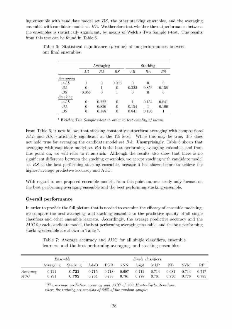
ing ensemble with candidate model set BS, the other stacking ensembles, and the averaging

ensemble with candidate model set BA. We therefore test whether the outperformance between

the ensembles is statistically significant, by means of Welch’s Two Sample t-test. The results

from this test can be found in Table 6.

Table 6: Statistical significance (p-value) of outperformances betweenour final ensembles

Averaging Stacking

All BA BS All BA BS

AveragingALL 1 0 0.056 0 0 0BA 0 1 0 0.222 0.856 0.158BS 0.056 0 1 0 0 0

StackingALL 0 0.222 0 1 0.154 0.841BA 0 0.856 0 0.154 1 0.106BS 0 0.158 0 0.841 0.106 1

I Welch’s Two Sample t-test in order to test equality of means

From Table 6, it now follows that stacking constantly outperform averaging with compositions

ALL and BS, statistically significant at the 1% level. While this may be true, this does

not hold true for averaging the candidate model set BA. Unsurprisingly, Table 6 shows that

averaging with candidate model set BA is the best performing averaging ensemble, and from

this point on, we will refer to it as such. Although the results also show that there is no

significant difference between the stacking ensembles, we accept stacking with candidate model

set BS as the best performing stacking ensemble, because it has shown before to achieve the

highest average predictive accuracy and AUC.

With regard to our proposed ensemble models, from this point on, our study only focuses on

the best performing averaging ensemble and the best performing stacking ensemble.

Overall performance

In order to provide the full picture that is needed to examine the efficacy of ensemble modeling,

we compare the best averaging- and stacking ensemble to the predictive quality of all single

classifiers and other ensemble learners. Accordingly, the average predictive accuracy and the

AUC for each candidate model, the best performing averaging ensemble, and the best performing

stacking ensemble are shown in Table 7.

Table 7: Average accuracy and AUC for all single classifiers, ensemblelearners, and the best performing averaging- and stacking ensembles

Ensemble Single classifiers

Averaging Stacking AdaB EGB kNN Logit MLP NB SVM RF

Accuracy 0.721 0.722 0.715 0.718 0.697 0.712 0.714 0.681 0.714 0.717AUC 0.791 0.792 0.784 0.788 0.761 0.778 0.781 0.730 0.776 0.785

I The average predictive accuracy and AUC of 200 Monte-Carlo iterations,where the training set consists of 80% of the random sample

28

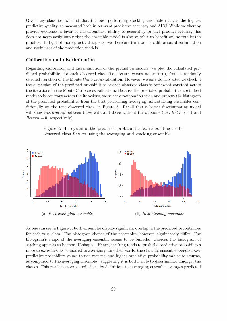
Given any classifier, we find that the best performing stacking ensemble realizes the highest

predictive quality, as measured both in terms of predictive accuracy and AUC. While we thereby

provide evidence in favor of the ensemble’s ability to accurately predict product returns, this

does not necessarily imply that the ensemble model is also suitable to benefit online retailers in

practice. In light of more practical aspects, we therefore turn to the calibration, discrimination

and usefulness of the prediction models.

Calibration and discrimination

Regarding calibration and discrimination of the prediction models, we plot the calculated pre-

dicted probabilities for each observed class (i.e., return versus non-return), from a randomly

selected iteration of the Monte Carlo cross-validation. However, we only do this after we check if

the dispersion of the predicted probabilities of each observed class is somewhat constant across

the iterations in the Monte Carlo cross-validation. Because the predicted probabilities are indeed

moderately constant across the iterations, we select a random iteration and present the histogram

of the predicted probabilities from the best performing averaging- and stacking ensembles con-

ditionally on the true observed class, in Figure 3. Recall that a better discriminating model

will show less overlap between those with and those without the outcome (i.e., Return = 1 and

Return = 0, respectively).

Figure 3: Histogram of the predicted probabilities corresponding to theobserved class Return using the averaging and stacking ensemble

(a) Best averaging ensemble (b) Best stacking ensemble

As one can see in Figure 3, both ensembles display significant overlap in the predicted probabilities

for each true class. The histogram shapes of the ensembles, however, significantly differ. The

histogram’s shape of the averaging ensemble seems to be bimodal, whereas the histogram of

stacking appears to be more U-shaped. Hence, stacking tends to push the predictive probabilities

more to extremes, as compared to averaging. In other words, the stacking ensemble assigns lower

predictive probability values to non-returns, and higher predictive probability values to returns,

as compared to the averaging ensemble - suggesting it is better able to discriminate amongst the

classes. This result is as expected, since, by definition, the averaging ensemble averages predicted

29

probabilities of the candidate models, whereas the stacking ensemble attempts to correct for

outliers in the predicted probabilities of each candidate model.

However, both ensemble combining methods appear to return biased probabilities, namely,

the histograms show peaks around 0.1 and 0.9 predicted probability, while predicted probabilities

close to 0 or 1 are either very rare or not even observed. A possible explanation of the difficulty

the ensembles have in making predictions close to 0 and 1 could be that, variance in the

underlying candidate models tend to move predictions, that should be approximating 0 or 1,

away from these values. This bias caused by variance, in turn, tend to be one-sided close to 0

and 1, because predictions are restricted to the interval [0,1]. As an example, for an ensemble to

calculate a predicted probability of 0, every single candidate model has to calculate a predicted

probability of 0. In this case, noise in the candidate models that the ensemble combines, results

in predicted values larger than 0, and hence, moves the predicted probability of the ensemble

away from 0.

To provide more insight in the dynamics of the candidate models within the ensembles,

we present visualizations of the predictive probabilities of the eight candidate models in Figure

A.4, given in the appendix. These figures also give more understanding in the calibration and

discriminative ability of each candidate model. They show, for example, the diversity between

the candidate models in these aspects. But, more importantly, for most candidate models, they

also show that predicted probabilities close to 0 or 1 are either very rare or not observed -

suggesting that most candidate models return biased probabilities. In fact, the logistic regression

appears to be the only candidate model that is properly calibrated. This provides an additional

explanation why the predicted probabilities of the best performing ensembles are hardly ever

close to 0 or 1.

Hence, we find evidence, although limited, that most candidate models and ensembles

are not well calibrated. They may be over- or underconfident when predicting a low or high

probability, suggesting that the predicted probability of an outcome does not reflect the real

world probability of that outcome. Consequently, a prediction model might predict that a

particular product purchase has a 80% probability of being returned, when in reality, the true

probability of the product being returned equals 90%.

Practical usefulness

As mentioned before, systems for prediction and prevention of product returns should focus on

extreme cases. On the basis of the testing set, we define the extreme cases by the 10%- and 15%

thresholds, such that for these thresholds, the purchases that are expected to be most likely to

result in a return, are evaluated. The results are reported in Table 8.

Some classification algorithms, however, including the support vector machine, do not

provide a probabilistic interpretation. Therefore we transform the output of the SVM first,

before we interpret the results, where we follow a procedure that uses a logistic regression to

map the SVM output to probabilities, proposed by Platt et al. (1999).

30

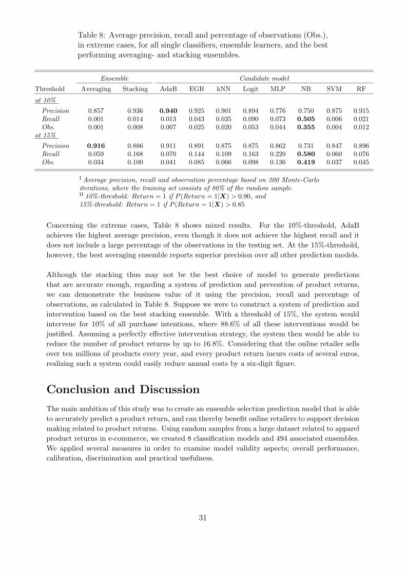
Table 8: Average precision, recall and percentage of observations (Obs.),in extreme cases, for all single classifiers, ensemble learners, and the bestperforming averaging- and stacking ensembles.

Ensemble Candidate model

Threshold Averaging Stacking AdaB EGB kNN Logit MLP NB SVM RF

at 10%

Precision 0.857 0.936 0.940 0.925 0.901 0.894 0.776 0.750 0.875 0.915Recall 0.001 0.014 0.013 0.043 0.035 0.090 0.073 0.505 0.006 0.021Obs. 0.001 0.008 0.007 0.025 0.020 0.053 0.044 0.355 0.004 0.012

at 15%

Precision 0.916 0.886 0.911 0.891 0.875 0.875 0.862 0.731 0.847 0.896Recall 0.059 0.168 0.070 0.144 0.109 0.163 0.220 0.580 0.060 0.076Obs. 0.034 0.100 0.041 0.085 0.066 0.098 0.136 0.419 0.037 0.045

I Average precision, recall and observation percentage based on 200 Monte-Carloiterations, where the training set consists of 80% of the random sample.II 10%-threshold: Return = 1 if P (Return = 1|X) > 0.90, and15%-threshold: Return = 1 if P (Return = 1|X) > 0.85

Concerning the extreme cases, Table 8 shows mixed results. For the 10%-threshold, AdaB

achieves the highest average precision, even though it does not achieve the highest recall and it

does not include a large percentage of the observations in the testing set. At the 15%-threshold,

however, the best averaging ensemble reports superior precision over all other prediction models.

Although the stacking thus may not be the best choice of model to generate predictions

that are accurate enough, regarding a system of prediction and prevention of product returns,

we can demonstrate the business value of it using the precision, recall and percentage of

observations, as calculated in Table 8. Suppose we were to construct a system of prediction and

intervention based on the best stacking ensemble. With a threshold of 15%, the system would

intervene for 10% of all purchase intentions, where 88.6% of all these interventions would be

justified. Assuming a perfectly effective intervention strategy, the system then would be able to

reduce the number of product returns by up to 16.8%. Considering that the online retailer sells

over ten millions of products every year, and every product return incurs costs of several euros,

realizing such a system could easily reduce annual costs by a six-digit figure.

Conclusion and Discussion

The main ambition of this study was to create an ensemble selection prediction model that is able

to accurately predict a product return, and can thereby benefit online retailers to support decision

making related to product returns. Using random samples from a large dataset related to apparel

product returns in e-commerce, we created 8 classification models and 494 associated ensembles.

We applied several measures in order to examine model validity aspects; overall performance,

calibration, discrimination and practical usefulness.

31

Theoretical conclusions

Our analysis demonstrated that the stacking ensemble which combines AdaB, EGB, MLP, NB,

SVM and RF together, is able to outperform any of the classification algorithms that we con-

sidered, in terms of predictive accuracy and AUC. In particular, the ensemble model predicted

product returns with average accuracy of 72.2%, which is 0.6% more accurate than the next best

single classification model; EGB. Furthermore, we showed that the ensemble model is able to

appropriately discriminate among purchases that do return and those that do not, despite some

evidence that the ensemble is not perfectly calibrated. Overall, the ensemble model was shown to

effectively identify consumption patterns associated with a high- or low rate of product returns.

Hence, corresponding to the first part of our main research question, “is an ensemble selection

prediction model based on customer-, product- and shopping basket specific characteristics able

to efficiently predict product returns?”, we conclude that it is, indeed, able to efficiently predict

product returns.

In addition, our analysis showed that several of the single classifiers that we considered

in our study were also able to generate accurate predictions. Namely, each of the single

classifiers, with the exception of KNN and NB, were able to predict product returns with an

average accuracy of at least 71% and at most 71.8%. Corresponding to our first sub-question,

“Is each of the individual prediction models able to efficiently predict product returns based

on customer-, product- and shopping basket specific characteristics?”, we therefore conclude

that AdaB, EGB, MLP, Logit, SVM and RF are all efficient in predicting product returns.

Corresponding to our second sub-question, “Is our proposed ensemble selection model more

efficient in predicting product returns, as compared to each individual prediction model?”, we

conclude that our proposed ensemble is, indeed, more efficient in predicting product returns as

compared to each individual prediction model.

Next to analyzing the efficacy of the diverse prediction models, our study demonstrated

that return decisions are influenced by customer-, product- and basket related characteristics. In

answer to our last sub-question, “How are product returns influenced by customer-, product- and

shopping basket specific characteristics?”, we conclude that, amongst others, gender and age,

product price and -quality, and the number of different product categories have a substantial

impact on the likelihood of a product return. Additionally, the analysis demonstrated that

several control variables, such as return deadlines as well as seasonality, also have an influence

on return decisions.

Practical implications

As the stacking ensemble achieved the highest predictive accuracy, the stacking ensemble turned

out to be especially useful to account for product returns when computing CLV. Moreover, our

analysis demonstrated the business value of the ensemble when used in a system of prediction and

prevention of product returns, that focuses only on purchases with a very high return probability.

To this end, the ensemble could constitute a meaningful contribution to online retailers’ overall

profit margins, even with a conservative intervention strategy. Whether and to what extent a

system of prediction and intervention should be implemented is, however, essentially a business

decision considering the fact that our stacking ensemble did not achieve the highest precision

compared to some other classifiers.

32

Hence, corresponding to the second part of our main research question, “Is the ensemble

model useful to support decision making processing related to product returns?”, we conclude

that it, indeed, can have practical usefulness.

Our study thus provided an accurate product prediction return model, establishing, that

several single classifier models compose good alternatives to it. Besides, it clearly showed that

any model aiming to efficiently predict product returns should take into account customer-,

product- and basket related variables. This knowledge is especially beneficial to online retailers

in their decision making and action taking in relation to product returns. It may ultimately

prompt online retailers to compose innovative return strategies in order to approach the, by

them desired, optimal return rate and minimize associated return costs. We do note though,

that, as the ensemble model and most single classifiers are not perfectly calibrated, a pure

probabilistic interpretation needs to approached with care.

Limitations

We do have to note, however, that the explanatory model resulting from our study has its

limitations and therefore would be most useful to particular online retailers specifically. First,

that is to say because the study solely focused on fashion products and did not take into account

other product types, such as electronica or furniture. Second, our study did not distinguish

between different fashion categories, whereas there appear to be significant differences in overall

return probabilities across product categories.

Our model does also not exclude features that only become available after purchase, such

as the payment method, and therefore cannot be used to predict the return probability before

a transaction takes place. For online retailers that would like to focus on identifying the

consumption patterns with a very high return rate before the transaction takes place, a model

that excludes these features would be more useful. However, excluding these features from the

model negatively influences the accuracy of the product return predictions, and we therefore

chose not to do so.

Recommendations

We recommend several routes to overcome these limitations and for further research. First, it is

recommended that future research on the explanatory model is extended to other merchandise

types. Second, it is recommended that further research is being done on the exact differences

in overall return probabilities across fashion product categories. Third, it is recommended that

further research into a model that excludes features that only become available after purchase

is being done. Additionally, more in depth research into further increasing the accuracy of the

ensemble model by including additional candidate models, and generating ensembles using other

strategies, such as the directed hill-climbing strategy (Caruana et al., 2004) and bagging strategy

(Breiman, 1996), is recommended.

33

References

Aguilar, Francisco X and Zhen Cai (2010). Conjoint effect of environmental labeling, disclosure

of forest of origin and price on consumer preferences for wood products in the us and uk.

Ecological Economics 70 (2), 308–316.

Akaike, Hirotugu (1974). A new look at the statistical model identification. IEEE transactions

on automatic control 19 (6), 716–723.

Akram, Umair, Peng Hui, Muhammad Kaleem Khan, Muhammad Hashim, and Sehrish Khan

Saduzai (2017). Impulsive buying: a qualitative investigation of the phenomenon. In Proceed-

ings of the Tenth International Conference on Management Science and Engineering Manage-

ment, pp. 1383–1399. Springer.

Anderson, Eric T, Karsten Hansen, and Duncan Simester (2009). The option value of returns:

Theory and empirical evidence. Marketing Science 28 (3), 405–423.

Anderson, Eric T, Karsten Hansen, Duncan Simester, and Lei K Wang (2008). How are demand

and returns related. Theory and empirical evidence 11, 70.

Bijmolt, Tammo HA, Alec Minnema, and Sander FM Beckers (2017). Return to sender! drivers

and consequences of online product returns.

Bjørner, Thomas Bue, Lars Garn Hansen, and Clifford S Russell (2004). Environmental labeling

and consumers’ choice—an empirical analysis of the effect of the nordic swan. Journal of

Environmental Economics and Management 47 (3), 411–434.

Breiman, Leo (1996). Bagging predictors. Machine learning 24 (2), 123–140.

Caruana, Rich, Alexandru Niculescu-Mizil, Geoff Crew, and Alex Ksikes (2004). Ensemble se-

lection from libraries of models. In Proceedings of the twenty-first international conference on

Machine learning, pp. 18. ACM.

Craney, Trevor A and James G Surles (2002). Model-dependent variance inflation factor cutoff

values. Quality Engineering 14 (3), 391–403.

David, Blanchard (2007). ”supply chains also work in reverse”. Industry Week .

De Langhe, Bart, Philip M Fernbach, and Donald R Lichtenstein (2015). Navigating by the stars:

Investigating the actual and perceived validity of online user ratings. Journal of Consumer

Research 42 (6), 817–833.

D’Souza, Clare, Mehdi Taghian, and Peter Lamb (2006). An empirical study on the influence

of environmental labels on consumers. Corporate communications: an international jour-

nal 11 (2), 162–173.

Fernandez-Delgado, Manuel, Eva Cernadas, Senen Barro, and Dinani Amorim (2014). Do we need

hundreds of classifiers to solve real world classification problems. J. Mach. Learn. Res 15 (1),

3133–3181.

34

Freeman, Elizabeth A and Gretchen G Moisen (2008). A comparison of the performance of

threshold criteria for binary classification in terms of predicted prevalence and kappa. Ecological

Modelling 217 (1-2), 48–58.

Freund, Yoav and Robert E Schapire (1997). A decision-theoretic generalization of on-line learn-

ing and an application to boosting. Journal of computer and system sciences 55 (1), 119–139.

Griffis, Stanley E, Shashank Rao, Thomas J Goldsby, and Tarikere T Niranjan (2012). The cus-

tomer consequences of returns in online retailing: An empirical analysis. Journal of Operations

Management 30 (4), 282–294.

Heilig, Leonard, Julien Hofer, Stefan Lessmann, and Stefan Voß (2016). Data-driven product

returns prediction: a cloud-based ensemble selection approach. In ECIS, pp. Research–in.

Hess, James D and Glenn E Mayhew (1997). Modeling merchandise returns in direct marketing.

Journal of Interactive Marketing 11 (2), 20–35.

Janakiraman, Narayan and Lisa Ordonez (2012). Effect of effort and deadlines on consumer

product returns. Journal of Consumer Psychology 22 (2), 260–271.

Janakiraman, Narayan, Holly A Syrdal, and Ryan Freling (2016). The effect of return policy

leniency on consumer purchase and return decisions: A meta-analytic review. Journal of

Retailing 92 (2), 226–235.

Kirmani, Amna and Akshay R Rao (2000). No pain, no gain: A critical review of the literature

on signaling unobservable product quality. Journal of marketing 64 (2), 66–79.

Kumar, Rajeev and Abhaya Indrayan (2011). Receiver operating characteristic (roc) curve for

medical researchers. Indian pediatrics 48 (4), 277–287.

Kuncheva, Ludmila I (2004). Combining pattern classifiers: methods and algorithms. John Wiley

& Sons.

Kutner, Michael H, Chris Nachtsheim, and John Neter (2004). Applied linear regression models.

McGraw-Hill/Irwin.

Lessmann, Stefan and Stefan Voß (2010). Customer-centric decision support. Business & Infor-

mation Systems Engineering 2 (2), 79–93.

Lin, Mingfeng, Henry C Lucas Jr, and Galit Shmueli (2013). Research commentary—too big to

fail: large samples and the p-value problem. Information Systems Research 24 (4), 906–917.

Liu, Canran, Pam M Berry, Terence P Dawson, and Richard G Pearson (2005). Selecting thresh-

olds of occurrence in the prediction of species distributions. Ecography 28 (3), 385–393.

Minnema, Alec, Tammo HA Bijmolt, Sonja Gensler, and Thorsten Wiesel (2016). To keep or

not to keep: Effects of online customer reviews on product returns. Journal of retailing 92 (3),

253–267.

Minnema, Alec, Tammo HA Bijmolt, J Andrew Petersen, and Jeffrey D Shulman (2018). Manag-

ing product returns within the customer value framework. In Customer Engagement Marketing,

pp. 95–118. Springer.

35

Monroe, Kent B (1973). Buyers’ subjective perceptions of price. Journal of marketing research,

70–80.

Partalas, Ioannis, Grigorios Tsoumakas, and Ioannis Vlahavas (2010). An ensemble uncertainty

aware measure for directed hill climbing ensemble pruning. Machine Learning 81 (3), 257–282.

Petersen, J Andrew and Eric T Anderson (2015). Leveraging product returns to maximize

customer equity. Handbook of research on customer equity in marketing , 177–160.

Petersen, J Andrew and V Kumar (2009). Are product returns a necessary evil? antecedents

and consequences. Journal of Marketing Research 73 (3), 35–51.

Platt, John et al. (1999). Probabilistic outputs for support vector machines and comparisons to

regularized likelihood methods. Advances in large margin classifiers 10 (3), 61–74.

R Core Team (2015). R: A Language and Environment for Statistical Computing. Vienna,

Austria: R Foundation for Statistical Computing.

Sahoo, Nachiketa, Chrysanthos Dellarocas, and Shuba Srinivasan (2018). The impact of online

product reviews on product returns. Information Systems Research.

Schwarz, Gideon et al. (1978). Estimating the dimension of a model. The annals of statistics 6 (2),

461–464.

Steyerberg, Ewout W, Andrew J Vickers, Nancy R Cook, Thomas Gerds, Mithat Gonen, Nancy

Obuchowski, Michael J Pencina, and Michael W Kattan (2010). Assessing the performance

of prediction models: a framework for some traditional and novel measures. Epidemiology

(Cambridge, Mass.) 21 (1), 128.

Stock, James, Thomas Speh, and Herbert Shear (2002). Many happy (product) returns.

Toktay, Beril (2001). Forecasting product returns. INSEAD.

Tsoumakas, Grigorios, Ioannis Partalas, and Ioannis Vlahavas (2008). A taxonomy and short

review of ensemble selection. In Workshop on Supervised and Unsupervised Ensemble Methods

and Their Applications.

Urbanke, Patrick, Johann Kranz, and Lutz Kolbe (2015). Predicting product returns in e-

commerce: The contribution of mahalanobis feature extraction.

Vergouwe, Yvonne (2003). Validation of clinical prediction models: theory and applications in

testicular germ cell cancer.

Wood, Stacy L (2001). Remote purchase environments: The influence of return policy leniency

on two-stage decision processes. Journal of Marketing Research 38 (2), 157–169.

Yu, Chien-Chih and Chen-Shu Wang (2008). A hybrid mining approach for optimizing returns

policies in e-retailing. Expert Systems with Applications 35 (4), 1575–1582.

36

Appendix

Individual algorithms

Adaptive Boosting

The AdaBoost algorithm, introduced by Freund and Schapire (1997), is a type of ensemble

learning method where multiple learners are employed to build a stronger learning algorithm.

AdaBoost works by choosing a base algorithm (e.g., decision trees) and iteratively improving

it by accounting for the incorrectly classified examples in the training set. This ensemble

technique is also known as boosting.

To put it briefly, the AdaBoost algorithm starts by predicting the original data set with

the first learner, where each observation has an equal weight. After the first learner is then

trained, the predictions are evaluated, and a higher weight is given to those data points that

have been predicted incorrectly. The next learner would focus thereby more on the misclassified

observations. Hence, while taking into account the higher weighted observations that are

created in the first step, the AdaBoost algorithm continues to predict with the second learner.

Similar to the first step, the second learner is evaluated and weights for incorrect predictions

are determined, where the next learner will account for these particular new weights while

making the predictions. Being an iterative process, these steps continue until a limit is reached

in the number of models to train (i.e., maximum iterations), or at a certain benchmark for

predictive accuracy. Hence, Adaboost generates a sequence of learners, each focusing on the

previous one’s errors.

In our study, we consider the so called ‘AdaBoost.M1’ algorithm. That is, the Ad-

aBoost algorithm with decision trees as the base algorithm. In order to find the ‘optimal’

number of iterations (or the number of decision trees to use) for which AdaBoost runs, we

compare the predictive accuracy, AUC and computation time of three different settings, namely

nadab ∈ (10, 20, 50).

Ultimately, using the same set of variables as the optimal explanatory model given in

equation 1, we deem setting the number of iterations equal to nadab = 50 as appropriate to

use. That is to say because with this number of iterations, the AdaBoost algorithm achieves

the highest predictive accuracy and AUC, while the computation time is still reasonable

(approximately 25 minutes).

Extreme Gradient Boosting

Extreme gradient boosting is a classification method based on the principles of gradient

boosting. Analogous to adaptive boosting, gradient boosting is a type of ensemble learning

method where multiple weak learners are converted into a single stronger learner. Although

adaptive- and gradient boosing algorithms follow the same fundamental theory, they substan-

tially differ on how they build the weak learners during the iterative process. In ther words,

these algorithms consider alternative ways to empathize difficult instances.

In particular, instead of focusing on weighting wrongly predicted instances, as is done in

adaptive boosting, gradient boosting focuses on the difference between the observed- and

37

predicted value of the dependent variable, or so called residuals. In brief, gradient boosting

determines, in each iteration, the residuals and, in turn, fits another weak learner to these

residuals. The contribution of the weak learner to the strong learner is then determined using a

gradient descent optimization process, where the calculated contribution is the one minimizing

the overall error of the strong learner.

Essentially, gradient boosting calculates the gradient of the loss function with respect to the

prediction and this way generates an extra ‘helper prediction’ to enhance the prediction and

push the weak prediction closer and closer to the true outcome. Therefore, gradient boosting is

prone to over-fitting the data.

Finally, extreme gradient boosting is an advanced implementation of the gradient boost-

ing algorithm with regularization in order to avoid overfitting. The extreme gradient boosting

algorithm uses multiple parameters, where, in turn, parameter tuning is necessary in order to

improve the predictive quality.

To this extent, using the same set of variables as the optimal explanatory model given

in equation 1, we apply a grid search. The principle of grid search is, essentially, to use

cross-validation in order to evaluate a set of models, which differ from each other in their

parameter values, lying on a grid.

Ultimately, we find that the parameter set with the best performance is given by: num-

ber of iterations negb = 14, Learning Rate λegb = 0.3 and Maximum tree depth tegb = 6. The

set of independent variables that we use to train extreme gradient boosting is the same set of

variables as the optimal explanatory model given in equation 1.

k Nearest Neighbors

The k Nearest Neighbor (KNN) algorithm is a non-parametric classification method that predicts

a particular class based on the k closest points to an observation. The KNN algorithm then

simply determines the predicted class by a majority vote of these closest points. For instance, if

k = 1, the predicted class equals the same class of the single nearest neighbor. Consequently, the

choice of the parameter k is very crucial in this algorithm, where the best choice of k depends

upon the data.

The presence of noisy and irrelevant features, or feature scales that are not consistent with

their importance, severely affects the performance of KNN. Therefore, scaling the features may

improve classification. In our study, we normalize the data using the Min-Max normalization

given by,

zi =xi −min(x)

max(x)−min(x), (3)

where x = (x1, . . . , xn) and zi is the ith normalized data from n observations.

Eventually, the variables we include in KNN are Ordersize Fashion, Price, Discount ratio,

Discountpermanent, Discount temporary, Voucher, NoFreeShipping, PastReturnRateProduct,

PastReturnRateCustomer and an interaction term calculated as

ReturnRates = PastReturnRateProduct × PastReturnRateCustomer.

38

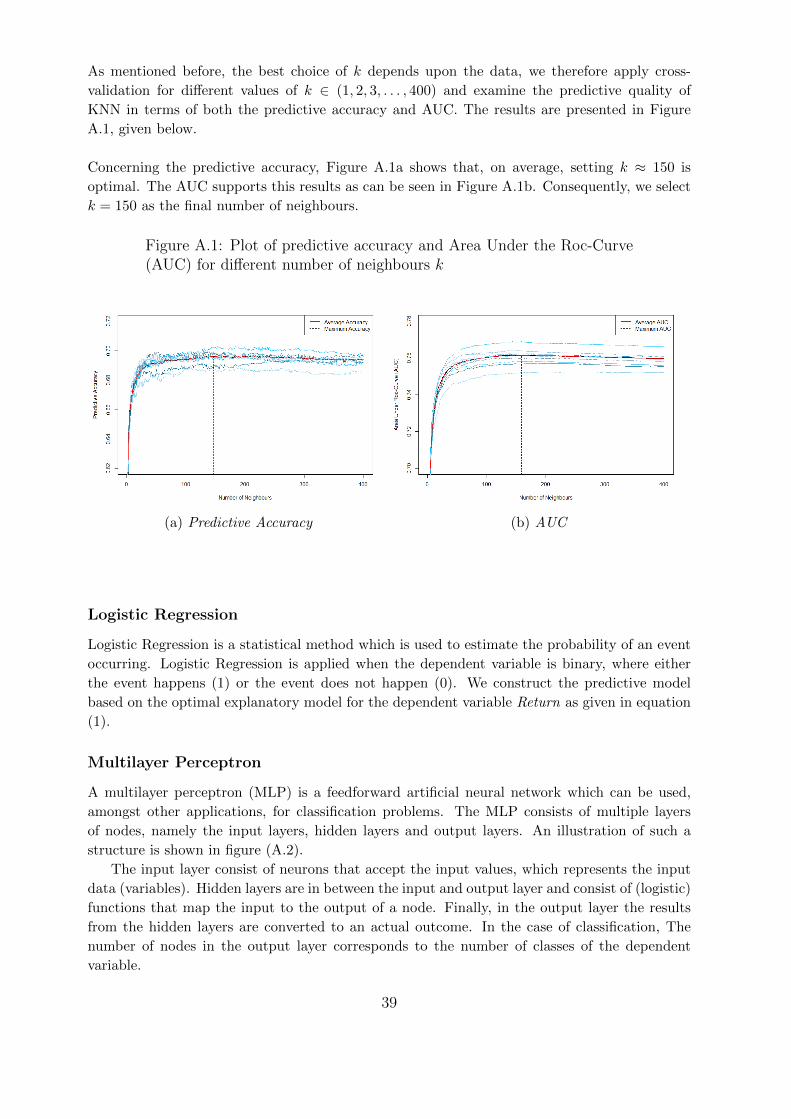
As mentioned before, the best choice of k depends upon the data, we therefore apply cross-

validation for different values of k ∈ (1, 2, 3, . . . , 400) and examine the predictive quality of

KNN in terms of both the predictive accuracy and AUC. The results are presented in Figure

A.1, given below.

Concerning the predictive accuracy, Figure A.1a shows that, on average, setting k ≈ 150 is

optimal. The AUC supports this results as can be seen in Figure A.1b. Consequently, we select

k = 150 as the final number of neighbours.

Figure A.1: Plot of predictive accuracy and Area Under the Roc-Curve(AUC) for different number of neighbours k

(a) Predictive Accuracy (b) AUC

Logistic Regression

Logistic Regression is a statistical method which is used to estimate the probability of an event

occurring. Logistic Regression is applied when the dependent variable is binary, where either

the event happens (1) or the event does not happen (0). We construct the predictive model

based on the optimal explanatory model for the dependent variable Return as given in equation

(1).

Multilayer Perceptron

A multilayer perceptron (MLP) is a feedforward artificial neural network which can be used,

amongst other applications, for classification problems. The MLP consists of multiple layers

of nodes, namely the input layers, hidden layers and output layers. An illustration of such a

structure is shown in figure (A.2).

The input layer consist of neurons that accept the input values, which represents the input

data (variables). Hidden layers are in between the input and output layer and consist of (logistic)

functions that map the input to the output of a node. Finally, in the output layer the results

from the hidden layers are converted to an actual outcome. In the case of classification, The

number of nodes in the output layer corresponds to the number of classes of the dependent

variable.

39

Figure A.2: An example of a Multilayer Perceptron architecture

In order to secure the ability of the MLP to generalize, the number of hidden nodes has to be kept

as low as possible. For a large excess of nodes, the MLP becomes a memory bank which can recall

the training set to perfection, but does not perform well on samples that outside the training set.

We consider a maximum of two hidden layers, because they can represent an arbitrary

decision boundary to arbitrary accuracy with rational activation functions and can approximate

any smooth mapping to any accuracy.

Moreover, neural networks require the input to be scaled in a consistent way, where we

will again use Min-Max normalization as given in equation (3).

Using grid search, with parameter setting as given in Table 3, we find that the number

of layers equal to l = 2, with the hidden nodes in each layer h = 5 and a maximum of iterations

mmlp = 50 yield the best results, for the same set of variables as the optimal explanatory model

given in equation 1.

Naive Bayes

The Naive Bayes (NB) algorithm is a classification method that predict classes based on

Bayes’ theorem of probability with an assumption of independence among predictors. In other

words, the Naive Bayes classifier assumes that the presence of a particular feature in a class is

unrelated to the presence of any other feature.

In more detail, Bayes theorem provides a way of calculating posterior probability P (c|x)

from P (c), P (x) and P (x|c), namely,

P (c|x) =P (x|c)P (c)

P (x), where (4)

P (c|x) denotes the posterior probability of class c given predictor x,

P (c) denotes the prior probability of the class c,

P (x|c) denotes the likelihood which is the probability of the predictor given the class,

P (x) denotes the prior probability of the predictor x.

40

When a class of a categorical predictor is not observed in the data used to train the Naive

Bayes model, we have that P (x) = 0. However, if one does observe this class when making a

prediction, it turns out that the Naive Bayes model is unable to make a prediction (as can be

seen from equation (4)). This problem is also known as the Zero-Frequency problem.

In order to solve this, one can use smoothing techniques. Basically, employing smoothing

shifts some of the probability from the observed classes to the unseen classes. One of the

simplest smoothing techniques is the so called Laplace estimation, which is also included in this

study.

The major advantage of the Naive Bayes model is that it is straightforward and useful

for very large data sets. It performs especially well when the assumption of independence holds.

In real life, however, it rarely occurs that a set of predictors is completely independent.

Because of this assumption, we do not include many variables for the NB. Especially,

we will use the same set of variables as considered by the KNN.

Support Vector Machine

A Support Vector Machine (SVM) is a supervised machine learning algorithm that is commonly

used in classification problems. The basic principle of SVMs is to find a hyperplane that best

divides the dataset into classes. One can think of a hyperplane as a line that (linearly) separates

and thereby classifies a set of data.

However, most classification tasks are not that simple, and often more complex structures

are needed in order to make an optimal separation. It usually happens that the classes to

discriminate in the data are not linearly separable in a particular dimensional space. For this

reason, SVMs can map the data into higher dimensions by using a kernel function. The use of

kernel function allows much more complex discrimination between sets which are not convex at

all in the original space. For a set of independent variables Xi, there are number of kernels that

can be used in SVMs. These kernel functions include linear, polynomial, radial basis function

(RBF), and sigmoid:

K(Xi,Xj) =

XiXj Linear

(γXiXj + C)d Polynomial

exp(−γ|Xi −Xj |2) RBF

tanh(γXiXj + C) sigmoid,

(5)

where γ denotes the inverse of the standard deviation of the RBF kernel (γ > 0), and C is the

capacity constant (C ≥ 0). Note that the larger the C, the more the error is penalized, and

large values for γ leads to high bias and low variance models, and vice-versa.

Because SVMs are extended versions of linear classifiers, where classes may not be lin-

early separable, SVMs yield usually accurate predictions. Nevertheless, due to the fact that the

computation times can be high, it is not well suited to larger datasets.

In the end, we will use the same set of variables as the optimal explanatory model

given in equation 1, and select the RBF kernel function and γ = 1/(dimension(dataset)).

41

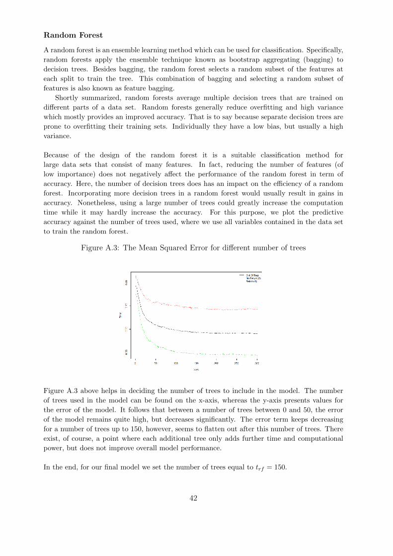
Random Forest

A random forest is an ensemble learning method which can be used for classification. Specifically,

random forests apply the ensemble technique known as bootstrap aggregating (bagging) to

decision trees. Besides bagging, the random forest selects a random subset of the features at

each split to train the tree. This combination of bagging and selecting a random subset of

features is also known as feature bagging.

Shortly summarized, random forests average multiple decision trees that are trained on

different parts of a data set. Random forests generally reduce overfitting and high variance

which mostly provides an improved accuracy. That is to say because separate decision trees are

prone to overfitting their training sets. Individually they have a low bias, but usually a high

variance.

Because of the design of the random forest it is a suitable classification method for

large data sets that consist of many features. In fact, reducing the number of features (of

low importance) does not negatively affect the performance of the random forest in term of

accuracy. Here, the number of decision trees does has an impact on the efficiency of a random

forest. Incorporating more decision trees in a random forest would usually result in gains in

accuracy. Nonetheless, using a large number of trees could greatly increase the computation

time while it may hardly increase the accuracy. For this purpose, we plot the predictive

accuracy against the number of trees used, where we use all variables contained in the data set

to train the random forest.

Figure A.3: The Mean Squared Error for different number of trees

Figure A.3 above helps in deciding the number of trees to include in the model. The number

of trees used in the model can be found on the x-axis, whereas the y-axis presents values for

the error of the model. It follows that between a number of trees between 0 and 50, the error

of the model remains quite high, but decreases significantly. The error term keeps decreasing

for a number of trees up to 150, however, seems to flatten out after this number of trees. There

exist, of course, a point where each additional tree only adds further time and computational

power, but does not improve overall model performance.

In the end, for our final model we set the number of trees equal to trf = 150.

42

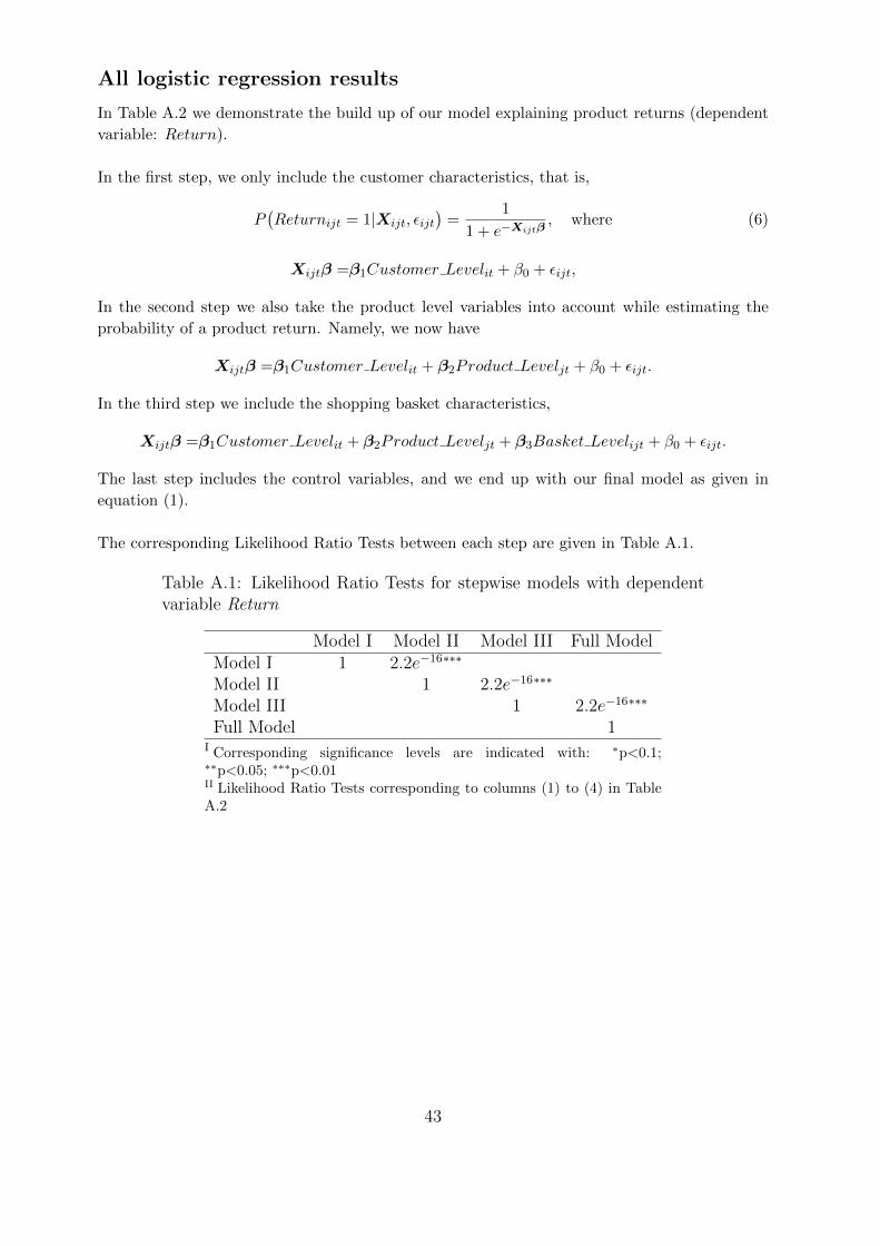
All logistic regression results

In Table A.2 we demonstrate the build up of our model explaining product returns (dependent

variable: Return).

In the first step, we only include the customer characteristics, that is,

P(Returnijt = 1|Xijt, εijt

)=

1

1 + e−Xijtβ, where (6)

Xijtβ =β1Customer Levelit + β0 + εijt,

In the second step we also take the product level variables into account while estimating the

probability of a product return. Namely, we now have

Xijtβ =β1Customer Levelit + β2Product Leveljt + β0 + εijt.

In the third step we include the shopping basket characteristics,

Xijtβ =β1Customer Levelit + β2Product Leveljt + β3Basket Levelijt + β0 + εijt.

The last step includes the control variables, and we end up with our final model as given in

equation (1).

The corresponding Likelihood Ratio Tests between each step are given in Table A.1.

Table A.1: Likelihood Ratio Tests for stepwise models with dependentvariable Return

Model I Model II Model III Full ModelModel I 1 2.2e−16∗∗∗

Model II 1 2.2e−16∗∗∗

Model III 1 2.2e−16∗∗∗

Full Model 1I Corresponding significance levels are indicated with: ∗p<0.1;∗∗p<0.05; ∗∗∗p<0.01II Likelihood Ratio Tests corresponding to columns (1) to (4) in TableA.2

43

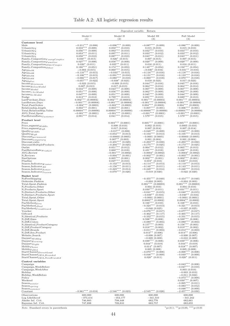
Table A.2: All logistic regression results

Dependent variable: Return

Model I Model II Model III Full Model(1) (2) (3) (4)

Customer levelMale −0.211∗∗∗ (0.008) −0.096∗∗∗ (0.009) −0.087∗∗∗ (0.009) −0.086∗∗∗ (0.009)Urbanicity2 0.033∗∗∗ (0.009) 0.050∗∗∗ (0.010) 0.015 (0.010) 0.015 (0.010)Urbanicity3 0.056∗∗∗ (0.009) 0.092∗∗∗ (0.010) 0.032∗∗∗ (0.010) 0.033∗∗∗ (0.010)Urbanicity4 0.053∗∗∗ (0.011) 0.097∗∗∗ (0.011) 0.033∗∗∗ (0.012) 0.033∗∗∗ (0.012)Urbanicity5 0.058∗∗∗ (0.010) 0.087∗∗∗ (0.010) 0.043∗∗∗ (0.011) 0.043∗∗∗ (0.011)Family CompostionY oungCouples 0.030∗∗ (0.015) 0.026∗ (0.015) 0.007 (0.015) 0.007 (0.015)Family CompostionFamilies 0.027∗∗∗ (0.008) 0.058∗∗∗ (0.009) 0.029∗∗∗ (0.009) 0.029∗∗∗ (0.009)Family CompostionOlderCoupes 0.020∗ (0.011) 0.025∗∗ (0.011) 0.016 (0.011) 0.016 (0.011)Family CompostionOther 0.180∗∗∗ (0.051) 0.174∗∗∗ (0.053) 0.149∗∗∗ (0.054) 0.150∗∗∗ (0.054)Age25to34 −0.003 (0.015) 0.060∗∗∗ (0.015) −0.030∗ (0.016) −0.031∗∗ (0.016)Age35to44 −0.110∗∗∗ (0.015) −0.033∗∗ (0.015) −0.116∗∗∗ (0.016) −0.118∗∗∗ (0.016)Age45to54 −0.106∗∗∗ (0.015) −0.091∗∗∗ (0.016) −0.131∗∗∗ (0.016) −0.133∗∗∗ (0.016)Age55to64 −0.066∗∗∗ (0.017) −0.080∗∗∗ (0.018) −0.069∗∗∗ (0.018) −0.070∗∗∗ (0.018)Age65plus −0.057∗∗∗ (0.022) −0.038∗ (0.023) 0.018 (0.023) 0.017 (0.023)IncomeMinimum −0.023 (0.015) −0.009 (0.015) 0.044∗∗∗ (0.016) 0.045∗∗∗ (0.016)IncomeBelowModal 0.007 (0.013) 0.017 (0.013) 0.064∗∗∗ (0.014) 0.064∗∗∗ (0.014)IncomeModal 0.034∗∗∗ (0.009) 0.043∗∗∗ (0.009) 0.067∗∗∗ (0.009) 0.067∗∗∗ (0.009)Income1.5×Modal 0.051∗∗∗ (0.008) 0.056∗∗∗ (0.009) 0.062∗∗∗ (0.009) 0.062∗∗∗ (0.009)Income2×Modal 0.047∗∗∗ (0.009) 0.051∗∗∗ (0.009) 0.045∗∗∗ (0.009) 0.044∗∗∗ (0.009)Nudge 0.813∗∗∗ (0.012) 0.799∗∗∗ (0.013) 0.691∗∗∗ (0.013) 0.689∗∗∗ (0.013)LastPurchase Days 0.002∗∗∗ (0.00004) 0.002∗∗∗ (0.00004) 0.001∗∗∗ (0.00004) 0.001∗∗∗ (0.00004)LastReturn Days −0.001∗∗∗ (0.00004) −0.001∗∗∗ (0.00004) −0.001∗∗∗ (0.00004) −0.001∗∗∗ (0.00004)Total PastOrders −0.004∗∗∗ (0.0003) −0.003∗∗∗ (0.0003) 0.004∗∗∗ (0.0003) 0.004∗∗∗ (0.0003)Relationship length 0.002∗∗∗ (0.001) 0.003∗∗∗ (0.001) −0.007∗∗∗ (0.001) −0.006∗∗∗ (0.001)Total RelationShip Value 0.00004∗∗∗ (0.00000) 0.00004∗∗∗ (0.00000) −0.00000∗∗∗ (0.00000) −0.00001∗∗∗ (0.00000)AVG Total Spent −0.001∗∗∗ (0.0001) −0.001∗∗∗ (0.0001) −0.001∗∗∗ (0.0001) −0.001∗∗∗ (0.0001)PastReturnRateCustomer 2.091∗∗∗ (0.014) 2.041∗∗∗ (0.014) 1.579∗∗∗ (0.015) 1.579∗∗∗ (0.015)

Product levelPrice 0.004∗∗∗ (0.0001) 0.005∗∗∗ (0.0001) 0.005∗∗∗ (0.0001)Price segmentMiddle 0.008 (0.010) 0.002 (0.010) 0.0005 (0.010)Price segmentHigh 0.017 (0.014) 0.007 (0.014) 0.007 (0.014)QualityMiddle −0.017∗∗ (0.008) −0.049∗∗∗ (0.009) −0.049∗∗∗ (0.009)QualityHigh −0.054∗∗∗ (0.013) −0.104∗∗∗ (0.013) −0.105∗∗∗ (0.013)Discountpermanent −0.00003 (0.0005) −0.0001 (0.0005) −0.00003 (0.0005)Discounttemporary 0.007∗∗ (0.003) 0.001 (0.004) 0.001 (0.004)Discount ratio −0.455∗∗∗ (0.029) −0.293∗∗∗ (0.030) −0.293∗∗∗ (0.030)DiscountMultipleProducts −0.204∗∗∗ (0.025) −0.175∗∗∗ (0.025) −0.173∗∗∗ (0.025)Outlet 0.051∗∗∗ (0.012) 0.064∗∗∗ (0.012) 0.065∗∗∗ (0.013)PastReturnRateProduct 2.660∗∗∗ (0.018) 2.431∗∗∗ (0.018) 2.436∗∗∗ (0.018)AVG Review −0.001∗∗∗ (0.0002) −0.0004∗ (0.0002) −0.0004∗ (0.0002)N Reviews −0.004∗∗∗ (0.001) −0.002∗∗∗ (0.001) −0.003∗∗∗ (0.001)SizeOptions 0.005∗∗∗ (0.001) 0.002∗∗∗ (0.001) 0.002∗∗∗ (0.001)PlusSize 0.027∗∗∗ (0.010) 0.019∗ (0.010) 0.020∗∗ (0.010)Season IndicatorWinter −0.152∗∗∗ (0.013) −0.114∗∗∗ (0.013) −0.119∗∗∗ (0.013)Season IndicatorAll −0.158∗∗∗ (0.011) −0.140∗∗∗ (0.011) −0.143∗∗∗ (0.011)Season IndicatorZomer −0.223∗∗∗ (0.014) −0.249∗∗∗ (0.014) −0.246∗∗∗ (0.014)Season IndicatorTussen −0.070∗∗∗ (0.020) −0.019 (0.020) −0.022 (0.020)

Basket levelNoFreeShipping −0.455∗∗∗ (0.040) −0.454∗∗∗ (0.040)Ordersize Fashion −0.004 (0.003) −0.004 (0.003)Total Spent Fashion 0.001∗∗∗ (0.00003) 0.001∗∗∗ (0.00003)N Products Other 0.004 (0.010) 0.004 (0.010)N Products Sport 0.030∗∗∗ (0.011) 0.031∗∗∗ (0.011)N Distinct Products Other −0.041∗∗∗ (0.015) −0.040∗∗∗ (0.015)N Distinct Products Sport −0.039∗∗ (0.016) −0.040∗∗ (0.016)Total Spent Other −0.0001 (0.0001) −0.0001 (0.0001)Total Spent Sport 0.0005∗∗ (0.0002) 0.0004∗∗ (0.0002)PayMethodGiro 0.166∗∗∗ (0.010) 0.168∗∗∗ (0.010)PayMethodiDeal −0.324∗∗∗ (0.013) −0.321∗∗∗ (0.013)PayMethodCreaditcard −0.040 (0.025) −0.037 (0.025)Voucher −0.076∗∗∗ (0.017) −0.077∗∗∗ (0.017)Giftcard −0.462∗∗∗ (0.117) −0.465∗∗∗ (0.117)N Identical Products −0.332∗∗∗ (0.015) −0.331∗∗∗ (0.015)N Diff Sizes 0.598∗∗∗ (0.008) 0.599∗∗∗ (0.008)N Diff Colors −0.089∗∗∗ (0.004) −0.089∗∗∗ (0.004)N Identical ProductCategory 0.157∗∗∗ (0.003) 0.158∗∗∗ (0.003)N Diff ProductCategory 0.018∗∗∗ (0.002) 0.019∗∗∗ (0.002)N Diff Brands −0.011∗∗∗ (0.003) −0.012∗∗∗ (0.003)N Diff Sex Product 0.013∗∗ (0.006) 0.014∗∗ (0.006)Website Search −0.008 (0.007) −0.008 (0.007)DaypartMidday −0.009 (0.009) −0.010 (0.009)DaypartEvening 0.039∗∗∗ (0.008) 0.039∗∗∗ (0.008)DaypartNight 0.044∗∗ (0.019) 0.044∗∗ (0.019)MobilePhone 0.014∗ (0.007) 0.018∗∗ (0.007)MobileTablet 0.005 (0.008) 0.005 (0.008)StartChannelDirectLoad −0.070∗∗∗ (0.008) −0.068∗∗∗ (0.008)StartChannelSEA Branded −0.048∗∗∗ (0.009) −0.049∗∗∗ (0.009)StartChannelSEA NonBranded 0.020∗ (0.011) 0.020∗ (0.011)

Control variablesCampaign −0.043∗∗∗ (0.008)Campaign WeekBefore −0.047∗∗∗ (0.010)Campaign WeekAfter 0.003 (0.010)Holiday −0.003 (0.010)Holiday WeekBefore −0.011 (0.022)Policy −0.073∗∗∗ (0.009)Weekend 0.030∗∗∗ (0.007)Seasonwinter −0.065∗∗∗ (0.011)Seasonspring −0.083∗∗∗ (0.012)Seasonsummer −0.048∗∗∗ (0.009)Constant −0.961∗∗∗ (0.018) −2.546∗∗∗ (0.023) −2.545∗∗∗ (0.028) −2.457∗∗∗ (0.030)

Observations 600,000 600,000 600,000 600,000Log Likelihood −373,414 −354,177 −341,310 −341,242Akaike Inf. Crit. 746,883 708,448 682,776 682,661Bayesian Inf. Crit. 747,898 709,810 683,757 683,655

Note: Standard errors in parenthesis ∗p<0.1; ∗∗p<0.05; ∗∗∗p<0.01

44

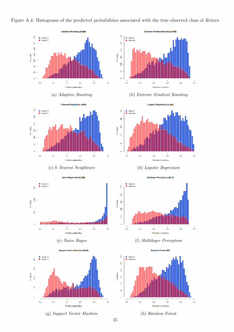
Figure A.4: Histograms of the predicted probabilities associated with the true observed class of Return

(a) Adaptive Boosting (b) Extreme Gradient Boosting

(c) k Nearest Neighbours (d) Logistic Regression

(e) Naive Bayes (f) Multilayer Perceptron

(g) Support Vector Machine (h) Random Forest

45