NOAA Technical Memorandum NMFS

JUNE 2005

PREDICTING THE POTENTIAL FOR HISTORICAL COHO, CHINOOK AND STEELHEAD HABITAT IN

NORTHERN CALIFORNIA

A. Agrawal R. S. Schick

E. P. Bjorkstedt R.G. Szerlong M. N. Goslin B. C. Spence T. H. Williams K. M. Burnett

NOAA-TM-NMFS-SWFSC-379

U.S. DEPARTMENT OF COMMERCE National Oceanic and Atmospheric Administration National Marine Fisheries Service Southwest Fisheries Science Center

NOAA Technical Memorandum NMFS

The National Oceanic and Atmospheric Administration (NOAA), organized in 1970, has evolved into an agency which establishes national policies and manages and conserves our oceanic, coastal, and atmospheric resources. An organizational element within NOAA, the Office of Fisheries is responsible for fisheries policy and the direction of the National Marine Fisheries Service (NMFS).

In addition to its formal publications, the NMFS uses the NOAA Technical

Memorandum series to issue informal scientific and technical publications when complete formal review and editorial processing are not appropriate or feasible. Documents within this series, however, reflect sound professional work and may be referenced in the formal scientific and technical literature.

NOAA Technical Memorandum NMFS This TM series is used for documentation and timely communication of preliminary results, interim reports, or special purpose information. The TMs have not received complete formal review, editorial control, or detailed editing.

JUNE 2005

PREDICTING THE POTENTIAL FOR HISTORICAL COHO, CHINOOK AND STEELHEAD HABITAT IN

NORTHERN CALIFORNIA

A. Agrawal1, R. S. Schick, E. P. Bjorkstedt, R. G. Szerlong, M. N. Goslin2, B. C. Spence, T. H. Williams, K. M. Burnett3

Santa Cruz Laboratory Southwest Fisheries Science Center

NOAA National Marine Fisheries Service 110 Shaffer Road

Santa Cruz, CA 95060

1Current Address: Center for GIS Research, California State Polytechnic University, 3801 W. Temple Ave., Pomona, CA 91768

2Current Address: Ecotrust, 721 Ninth Ave., Portland, OR 97209 3Aquatic and Land Interactions Program, Pacific Northwest Research Station, USDA Forest

Service, 3200 Jefferson Way, Corvallis, Oregon 97331

NOAA-TM-NMFS-SWFSC-379

U.S. DEPARTMENT OF COMMERCE Carlos M. Gutierrez, Secretary National Oceanic and Atmospheric Administration Vice Admiral Conrad C. Lautenbacher, Jr., Under Secretary for Oceans and Atmosphere National Marine Fisheries Service William T. Hogarth, Assistant Administrator for Fisheries

Contents

1 Introduction 1

2 Intrinsic potential: concept and general model 2

3 Implementation south of Cape Blanco 3

3.1 Generating stream networks and reach attributes . . . . . . . . . . . . . 3

3.2 Accounting for latitudinal gradients in climate . . . . . . . . . . . . . . . 5

3.3 Suitability curves . . . . . . . . . . . . . . . . . . . . . . . . . . . . . . . 6

3.3.1 Life history context for suitability curves . . . . . . . . . . . . . . 7

3.4 Example: Ten Mile River . . . . . . . . . . . . . . . . . . . . . . . . . . . 12

3.5 Temperature limitation for coho salmon. . . . . . . . . . . . . . . . . . . 12

3.6 Natural Barriers . . . . . . . . . . . . . . . . . . . . . . . . . . . . . . . . 13

4 Interpretation and appropriate use of intrinsic potential 13

5 Description of the GIS database 15

5.1 Distribution . . . . . . . . . . . . . . . . . . . . . . . . . . . . . . . . . . 15

5.2 Usage within a GIS . . . . . . . . . . . . . . . . . . . . . . . . . . . . . . 16

6 Acknowledgements 16

i

List of Tables

1 Sources of information synthesized through expert opinion to develop suit-

ability curves for ULEP, CLAMS, or this report. . . . . . . . . . . . . . . 11

ii

List of Figures

1 Suitability curves for each of the three IP components (Gradient, Val-

ley Constraint and Discharge) for juveniles of each of the three species

(coho, steelhead and chinook). Note the scale change (abscissa) across

each species for the gradient attribute. . . . . . . . . . . . . . . . . . . . 10

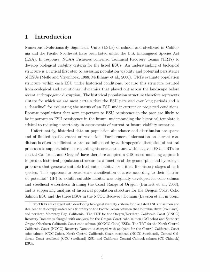
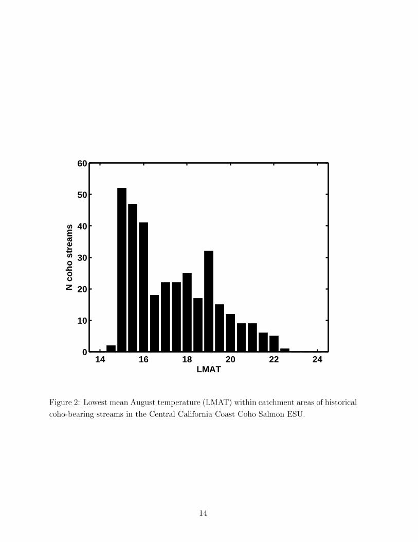
2 Lowest mean August temperature (LMAT) within catchment areas of his-

torical coho-bearing streams in the Central California Coast Coho Salmon

ESU. . . . . . . . . . . . . . . . . . . . . . . . . . . . . . . . . . . . . . . 14

iii

List of Plates

1 Intrinsic potential for coho salmon rearing habitat for the Ten Mile River. 22

2 Intrinsic potential for winter steelhead rearing habitat for the Ten Mile

River. . . . . . . . . . . . . . . . . . . . . . . . . . . . . . . . . . . . . . 23

3 Intrinsic potential for fall-run Chinook salmon spawning and rearing habi-

tat for the Ten Mile River. . . . . . . . . . . . . . . . . . . . . . . . . . . 24

4 Intrinsic potential for coho salmon rearing habitat in the Russian River

with areas from which coho salmon are likely to be excluded by high

summer temperatures. . . . . . . . . . . . . . . . . . . . . . . . . . . . . 25

iv

1 Introduction

Numerous Evolutionarily Significant Units (ESUs) of salmon and steelhead in Califor-

nia and the Pacific Northwest have been listed under the U.S. Endangered Species Act

(ESA). In response, NOAA Fisheries convened Technical Recovery Teams (TRTs) to

develop biological viability criteria for the listed ESUs. An understanding of biological

structure is a critical first step to assessing population viability and potential persistence

of ESUs (Meffe and Vrijenhoek, 1988; McElhany et al., 2000). TRTs evaluate population

structure within each ESU under historical conditions, because this structure resulted

from ecological and evolutionary dynamics that played out across the landscape before

recent anthropogenic disruption. The historical population structure therefore represents

a state for which we are most certain that the ESU persisted over long periods and is

a “baseline” for evaluating the status of an ESU under current or projected conditions.

Because populations that were important to ESU persistence in the past are likely to

be important to ESU persistence in the future, understanding the historical template is

critical to reducing uncertainty in assessments of current or future viability scenarios.

Unfortunately, historical data on population abundance and distribution are sparse

and of limited spatial extent or resolution. Furthermore, information on current con-

ditions is often insufficient or are too influenced by anthropogenic disruption of natural

processes to support inference regarding historical structure within a given ESU. TRTs for

coastal California and Oregon1 have therefore adopted a GIS-based modeling approach

to predict historical population structure as a function of the geomorphic and hydrologic

processes that generate suitable freshwater habitat for critical life-history stages of each

species. This approach to broad-scale classification of areas according to their “intrin-

sic potential” (IP) to exhibit suitable habitat was originally developed for coho salmon

and steelhead watersheds draining the Coast Range of Oregon (Burnett et al., 2003),

and is supporting analysis of historical population structure for the Oregon Coast Coho

Salmon ESU and the three ESUs in the NCCC Recovery Domain (Lawson et al., in prep.;

1Two TRTs are charged with developing biological viability criteria for five listed ESUs of salmon andsteelhead that occupy watersheds tributary to the Pacific Ocean between the Columbia River (exclusive),and northern Monterey Bay, California. The TRT for the Oregon/Northern California Coast (ONCC)Recovery Domain is charged with analyses for the Oregon Coast coho salmon (OC-coho) and SouthernOregon/Northern California Coast coho salmon (SONCC-Coho) ESUs. The TRT for the North-CentralCalifornia Coast (NCCC) Recovery Domain is charged with analyses for the Central California Coastcoho salmon (CCC-Coho), North-Central California Coast steelhead (NCCC-Steelhead), Central Cal-ifornia Coast steelhead (CCC-Steelhead) ESU, and California Coastal Chinook salmon (CC-Chinook)ESUs.

1

Bjorkstedt et al., in prep.).

In this report, we describe implementation of this approach to coastal watersheds

between Cape Blanco, Oregon, and Monterey Bay, California and characterize GIS data

sets developed for listed ESUs of salmon and steelhead in this region. Specifically, we

adapt the approach developed by Burnett et al. (2003) to predict IP for rearing habi-

tat of coho salmon (Oncorhynchus kisutch), winter steelhead (O. mykiss) and fall-run

Chinook salmon (O. tshawytscha). Note that we do not assess intrinsic potential for sum-

mer steelhead and spring-run Chinook salmon because these life-history strategies have

very specific habitat requirements (e.g., deep, cold pools in which the adults spend the

summer) that are not readily identified from available GIS data. In addition to the tech-

nical description of the model and analysis, we also offer guidance regarding appropriate

interpretation and use of these results in recovery planning for listed salmonids.

2 Intrinsic potential: concept and general model

The concept of a stream’s “intrinsic potential” to exhibit suitable habitat for a particular

species or life stage emanates from a hierarchical perspective of fish-habitat relationships

(sensu Frissell et al., 1986; Montgomery and Buffington, 1998). In this view, landform,

lithology, and hydrology interact to govern movement and deposition of sediment, large

wood, and other structural elements along a river network. These broader-scale charac-

teristics and processes thereby control gross channel morphology at the scale of stream

segments or reaches, as reflected in the frequency and characteristics of constituent habi-

tat units (e.g., pools, runs, riffles, side-channels, etc.). The IP concept assumes that this

hierarchy of organization, structure, and dynamics of physical habitat is reflected in the

biological organization of stream communities. In the case of salmonids, the biological re-

sponse manifests itself as heterogeneity in the distribution, abundance, and productivity

of different species and life stages within a stream network. The underlying framework

for the IP models assumes that three primary indicators of landform and hydrology —

channel gradient, an index of valley width, and mean annual discharge — reasonably

constrain channel morphology and hence the potential of a reach to express habitat con-

ditions favorable to a particular salmonid species at some stage of its life. These three

characteristics are effectively constant features of the landscape, and thus provide the

basis for predicting both potential habitat under historical conditions and the potential

for physical processes to recreate suitable habitat if left to operate more or less naturally.

Among-species or life-stage differences in habitat affinities are accommodated through

species-specific curves relating suitability to the three physical metrics.

2

Burnett et al. (2003) describe a practical model that translates stream reach charac-

teristics into a measure of intrinsic potential in two steps. First, reach-specific values for

each characteristic (i.e., gradient, valley constraint, and mean annual discharge) are con-

verted to habitat suitability scores through functions (“suitability curves”) that convert

the value of each variable to a scale of 0-1. Suitability curves are specific to species and

life-history stage (see §3.3 below). Second, reach-specific IP is calculated as the geometric

mean of reach-specific suitability scores for each of the three characteristics2. Combining

the marginal effects of each reach characteristic in this way is directly analogous to the

theoretical basis of a limiting factors analysis: a low value based on a single character-

istics will dramatically reduce or zero-out IP for a stream reach, and in these instances,

other reach characteristics are uninformative with respect to habitat potential.

3 Implementation south of Cape Blanco

In the following sections, we provide a brief overview of the basic approach outlined in

(Burnett et al., 2003), but focus in more detail on specific nuances of our implementation

of the IP model for watersheds south of Cape Blanco.

3.1 Generating stream networks and reach attributes

Calculating IP is a multi-step process that occurs both outside and inside a GIS. The first

step creates a stream network from the Digital Elevation Model (DEM) and precipitation

data that defines individual reaches and calculates values of gradient, valley floor width,

and discharge for each. The second step creates suitability curves for these three variables

based on life-history and habitat association of each species and life-stage. Finally, to

marry these two steps, Burnett et al. (2003) wrote a series of species-specific processing

scripts (Arc Macro Language, Environmental Systems Research Institute, Inc.3,4) to

2Mathematically, for stream reach k, IPk = 3√

fD(Dk) · fG(Gk) · fV (Vk), where Dk, Gk, and Vk aremean annual discharge, gradient, and valley constraint, respectively, of reach k, and each fx maps theappropriate characteristic x onto a scale of 0-1.

3Copyright c© 2005 ESRI. All rights reserved. ArcInfo is a trademark, registered trademark, or servicemark of ESRI in the United States, the European Community, or certain other jurisdictions

4Disclaimer of Endorsement: Reference to any specific commercial products, process, or service bytrade name, trademark, manufacturer, or otherwise, does not constitute or imply its endorsement,recommendation, or favoring by the United States Government. The views and opinions of authorsexpressed in this document do not necessarily state or reflect those of NOAA or of the United StatesGovernment, and shall not be used for advertising or product endorsement purposes.

3

calculate the IP score for each reach.

To construct a stream network, we implemented a model developed by Miller (2003)

that synthesizes grid-based data on topography derived from a 10 m resolution DEM5

and mean annual precipitation derived from the PRISM model (Daly et al., 1994)6. To

run the model (Miller, 2003) (which is implemented outside of a GIS in a series of For-

tran programs), we generated binary files of regional-scale elevation and precipitation

grids. Beginning with these grids, we clipped the DEM and precipitation files to the

watershed boundaries. The last input needed is a parameters file, and the only sub-

stantial change to the default inputs was to include regionally-specific equations relating

precipitation to discharge (See §3.2 for specifics). The model was run on a watershed by

watershed basis. Watersheds were defined a priori based on 1:100K hydrography (USGS

2003), sixth-field hydrologic unit code (HUC) boundaries (Fire and Resource Assessment

Program (FRAP), 1999; National Resources Conservation Service (NRCS), 2002), and

where required, manual delineation informed by topography. For very large basins (e.g.,

the Rogue, Klamath, and Eel rivers), it was necessary to model major tributaries and

sections of mainstem river separately, and subsequently to reassemble the basin in GIS7.

For each watershed, the model creates several output layers, including: Flow Direction

of the raster streams within the watershed using the Tarboton Method (Tarboton, 1997),

Flow Accumulation of the streams, and a vector version of the DEM derived streams

(whereby each reach includes information on the three variables that are the basis for

IP: gradient, valley constraint, and mean annual discharge).

In the course of constructing the stream network, the model dynamically defines

reaches on the order of 50-200 meters long, basing reach breaks on changes in gradient.

In the resulting stream network, each reach is characterized by its gradient (averaged over

510 m DEM coverage was not available for our entire study region at the time of analysis. Therefore,where seamless, original 10 m DEM coverage was not available, we generated a 10 m DEM by applyinga spline to interpolate a seamless 30 m resolution DEM to 10 m resolution. Comparisons of derivedproperties (e.g., stream gradient) aggregated at watershed scales, and the general structure of resultingwatersheds show negligible differences between analyses based on interpolated 10 m DEMs and analysesbased on independently derived 10 m DEMs.

6The PRISM data set is derived by interpolating climatic observations from the period 1961-1990 ata spatial resolution of 2km by 2km. The interpolation scheme accounts for the influence of elevation,aspect, and proximity to the coast on climatic variables such as temperature and precipitation (Dalyet al., 1994).

7The model (Miller, 2003) includes a Fortran routine to “stitch” the sub-watersheds back together.This routine matches stream topology during reassembly, and transfers discharge values from the streamat the outlet of the upstream watershed to the first reach in the downstream watershed.

4

the entire reach), valley width8, and mean annual discharge (calculated at the downstream

end of the reach).

Post processing on each of the three variables generated by the model also occurs

within the GIS; specifically, gradient is calibrated based on field measurements, discharge

is converted to metric units, and valley-floor width is used to generate the index of valley

constraint (Burnett et al., 2003)9

3.2 Accounting for latitudinal gradients in climate

By implementing the IP model directly, we assumed that geomorphic structure and

precipitation interact similarly to generate stream networks in northern California and

in coastal Oregon, for which the IP model was originally developed. We attempted

to evaluate this assumption by estimating regional models for mean annual discharge

as a function of catchment area and mean annual precipitation. To accomplish this,

we assembled discharge data for stream gages with at least 20 years of data during

the period for which the PRISM precipitation data were developed and with little or

no evidence of substantial upstream diversion, extraction or elevated evaporative loss10.

8Miller (2003) explains that valley floor width is “estimated as the length of a transect that intersectsthe valley walls at a specified height above the channel. Since the orientation of the valley is unknown,transect orientations is varied to find that which provides the minimum length. The height above thechannel is specified as 2.5 times estimated bank-full depth, given as a function of drainage area. Thevalue is currently coded in as Hbf = 0.36A0.2, where Hbf is bank-full depth and A is drainage area insquare kilometers (based on data in Benda (1994)). Thus the height above the channel from which thetransect is extended varies from a little less than a meter for small streams to a little over three metersfor large streams.”

9Burnett et al. (2003) derived an index of valley constraint by dividing valley floorwidth by active channel width, the latter of which was calculated as follows, ACW =2.19108 + 1.32366 ∗

√D, where D is mean annual discharge (in ft3/s). N.B. this Vk dif-

fers from the Vk enumerated in Oregon Department of Fish and Wildlife sampling protocol(http://gisweb.co.tillamook.or.us/library/standards/StreamHabitatMethods.pdf), in that this Vk is de-rived from a DEM as opposed to field based measurements. Because of this, our breaks in “constrained”and “unconstrained” are not arithmetically equivalent to ODFW’s, though they describe the same phe-nomenon. Note that the stream network and its attributes are the basis for all subsequent calculations,regardless of species or life-history stage.

10Gages were excluded on the basis of evidence of direct diversion extracted from Agajanian et al.(2002), Christy (2003), or USGS (2003). Estimates of extractions for irrigation were compiled fromestimates of irrigated area and HUC-level irrigation rates using information in Solley et al. (1998) andVogelman et al. (2000). Actual or estimated evaporation rates were used to evaluate losses from non-diversion reservoirs. If estimated evaporation rates or diversions for irrigation or water supply from thewatershed above a particular gage exceeded 2% of mean annual discharge, that gage was excluded from

5

Preliminary analyses indicated that the relation of mean annual discharge to catchment

area and mean annual precipitation in the SONCC Recovery Domain was essentially

identical to that for coastal Oregon. The final discharge-precipitation relationship we

developed for coastal watersheds throughout the study area was also very similar to that

used for coastal watersheds north of Cape Blanco11. On the basis of substantial climatic

differences, we estimated a separate model to predict discharge in watersheds in the San

Francisco Bay12.

3.3 Suitability curves

Suitability scores express the “likelihood” that suitable habitat will occur in a reach with

a particular value for a characteristic, independent of the value of the other characteris-

tics. In general, the form of the relationship between reach characteristics and habitat

suitability is not known precisely. What often is reasonably well known is the range of

values for a given characteristic that almost always yield favorable habitat as well as the

range of values for which favorable habitat almost never occurs. Given the uncertainty

associated with intermediate values, a simple linear relation is generally assumed to fill

in the gap between values corresponding to “good” and “poor” habitat potential. Note

that regardless of life-history stage, the upper extent of tiny positive values for gradient

reflects the ability of adults to ascend reaches of varying steepness, and thus defines the

range of accessible habitat.

Suitability curves are defined for each reach characteristic and for a species and life-

history stage. These functions are used to convert reach-specific values for each of the

three attributes to a scale of 0-1, and the resulting scores represent the effects of each

physical attribute on the potential of a stream reach to exhibit high quality habitat.

Our ability to measure “habitat quality” directly is extremely limited, and available data

sets, while informative, are generally insufficient to support extensive, rigorous statistical

estimation of the functional relationship between all three stream characteristics and

further analyses.11The final model for the region spanning coastal watersheds from Cape Blanco to Santa Cruz predicted

mean annual discharge, D (in m3s−1) according to ln(D) = −11.445 + 1.003 ln(A) + 1.467 ln(P ) (n =29, r2 = 0.988), where A is (planar) catchment area in ha and P is mean annual precipitation in mm.For comparison, the relation for coastal Oregon is ln(D) = −11.972 + 0.99 ln(A) + 1.593 ln(P ), whichwas taken directly from the Miller 2003 model. Note that these models are of the same form as thosedeveloped by the Oregon Department of Forestry (Lorensen et al., 1994).

12Based on data for San Francisco Bay and watersheds in the western Central Valley, we estimatedln(D) = −13.047 + 0.876 ln(A) + 2.171 ln(P ) (n = 20, r2 = 0.968).

6

their marginal effects on habitat quality. Suitability curves, therefore, represent expert

synthesis of data on fish distributions and abundance in the context of general habitat

requirements of a particular life-history stage of a particular species. Typically, such

syntheses are based on density estimates (e.g., the number of juvenile coho salmon per

100 m of stream), which are assumed to provide a measure of the amount of high quality

habitat in a reach, across a range of habitat characteristics. The assumption that habitat

suitability is proportional to use (i.e. density) in unmanaged systems extends well beyond

the studies where these models originated (the Umpqua Land Exchange Project (ULEP)

and Coastal Landscape Analysis and Modeling Study (CLAMS)), and is a basis for much

of ecology.

Figure 1 illustrates the suitability curves used to calculate IP for the relevant life

history stages of each of the three species addressed in this report. These curves are

based on those from CLAMS. Somewhat similarly, “index values” were developed in the

ULEP13. Table 1 provides some of the historical references used in the development of the

suitability curves, and additional data sets that we consulted when evaluating whether

relationships between stream characteristics and fish distributions provided evidence that

different suitability curves were required for our study region. With the exception of

Engle (2002), none of these data suggested that altering the curves for application to

California was warranted. Based on Engle’s (2002) work, we extended the range of

gradients that were accessible to adult steelhead and consistent with high likelihood of

suitable habitat for juvenile steelhead (Figure 1). We also reduced slightly the suitability

of highly constrained reaches for juvenile steelhead to recognize that these fish use (and

perform well in) habitats such as pools that are less common in highly constrained reaches.

3.3.1 Life history context for suitability curves

Understanding the ecology and habitat requirements of a given species at its various life

history stages is useful for interpreting and understanding the distribution of IP scores

within a basin. We therefore provide below a brief description for the relevant life history

stage for each of the species addressed in this report.

Juvenile coho salmon Juvenile coho salmon spend at least one summer and one win-

ter in freshwater, although some individuals may spend an additional year in freshwater.

13CLAMS and ULEP differed in that CLAMS used a geometric mean to calculate IP whereas ULEPuse an arithmetic mean. ULEP used discrete classes for the three attributes rather than suitabilitycurves. ULEP also did not attempt to interpret IP and actual habitat conditions separately. Lastly,CLAMS and ULEP interpret constraint for steelhead differently.

7

These fish exhibit traits, such as relatively large fins and laterally compressed bodies,

that are believed to be adaptations to living in the slower-velocity habitats where they

most commonly occur. During the summer, juvenile coho salmon generally prefer pool

habitats over runs and riffles (Bisson et al., 1988). Juvenile coho salmon often move out of

the main channel and seek refuge in side channels, alcoves, and other off-channel habitats

during periods of high stream discharge (Tschaplinski and Hartman, 1983; Meehan and

Bjornn, 1991; Bell et al., 2001). Together, these attributes and behaviors likely explain

why juveniles are most abundant in low-gradient (usually <2%-3% but occasionally up

to 5%), unconstrained reaches as opposed to constrained reaches or steeper headwater

streams.

The suitability curves that form the basis of IP predictions for juvenile coho salmon

reflect the likelihood that stream reaches will exhibit substantial pool and off-channel

habitat as a function of their geomorphological and hydrological characteristics (Figure

1a-c). These suitability curves are identical to those used by Lawson et al. (in prep.) to

predict IP for watersheds in coastal Oregon.

Juvenile (winter) steelhead The juvenile phase spans at least one summer and one

winter in freshwater, but is more variable and of greater maximum duration than is ob-

served for coho salmon. Following emergence in spring, steelhead fry typically adopt

feeding stations in shallower portions of riffles or pools, moving into progressively faster

and deeper water as they grow (Bisson et al., 1988). Juvenile steelhead exhibit a stream-

lined body morphology that is thought to be an adaptation for life in faster water currents

(Bisson et al., 1988). Although steelhead tend to prefer and grow faster in pool habitats,

as young-of-the-year, they are commonly displaced to riffle habitats through competi-

tive interactions with larger, more aggressive coho salmon when the latter are abundant

(Bugert and Bjornn, 1991; Young, 2004). Such displacement is not observed for older,

larger juvenile steelhead. The spawning distribution of steelhead overlaps with that of

coho salmon; however, because steelhead tend to prefer higher gradients (generally 2-7%,

though they may be found in reaches with gradients up to 12% or more), their distribu-

tion tends to extend farther upstream. In some watersheds, steelhead will even spawn in

ephemeral streams, with juveniles migrating downstream to permanent waters to rear.

The suitability curves that form the basis of IP predictions for juvenile steelhead

reflect the likelihood that stream reaches will exhibit substantial higher-energy habitats

as a function of their geomorphological and hydrological characteristics (Figure 1d-f). To

some degree, these curves implicitly include the consequences of ecological interactions

with coho salmon; however, these interactions take place at local scales, and in most if not

8

all cases where juvenile coho salmon occur, they are sympatric with juvenile steelhead at

the reach scale. Note that although we found no support for implementing a temperature-

based constraint on the predicted distribution of steelhead in our study area14, juvenile

steelhead are not likely to experience substantial “competitive release” with respect to

the distribution of high quality habitat in areas where coho salmon are excluded by

temperature. Instead, because the metabolic demands of juvenile steelhead increase

with temperature, it is likely that juvenile steelhead will continue to favor higher velocity

habitats that provide a greater rate of drift to supply their increased foraging needs

(Smith and Li, 1983).

Juvenile Fall-run Chinook salmon Fall-run Chinook salmon occur in rain-dominated

systems or the lower portions of systems with both rain and snowmelt influence, and tend

to spawn in low-gradient reaches with greater discharge that are somewhat lower in a

watershed than reaches used by steelhead. Ocean-type juveniles, which are typical of fall-

run populations, may begin migrating toward sea within a few weeks to a few months

of emergence, but some individuals may reside in streams through the summer months,

before moving to estuaries during the fall or winter (Reimers, 1973; Healy, 1991; Moyle,

2002).

The suitability curves that form the basis of IP predictions for fall-run Chinook salmon

reflect the dominance of gradient and discharge in determining where suitable habitats

are likely to occur (Figure 1g-i). Valley constraint is less important for juvenile Fall-run

Chinook, because juveniles have already gone to sea (in contrast to coho, which reside a

full year in fresh water), by the time winter high-flows occur.

14Analysis of environmental predictors of presence for steelhead in the South-Central California CoastESU (D. Boughton, NOAA Fisheries, Santa Cruz Lab, unpublished results) suggests that mean Augustair temperature exceeding 24 ◦C might limit the distribution of steelhead, a value corroborated by similaranalysis of the effects of water temperature on presence of O. mykiss (Eaton et al., 1995). Very little ofour study area experiences these conditions.

9

c(−1, 1)

Sui

tabi

lity

●

● ●

0 1 2 3 4 5 6 7

0.0

0.2

0.4

0.6

0.8

1.0

● ●

● ●

0 2 4 6 8

0.0

0.2

0.4

0.6

0.8

1.0

Coho

●

●● ●

●

0 20 40 60 80 100

0.0

0.2

0.4

0.6

0.8

1.0

c(−1, 1)

Sui

tabi

lity

●

● ●

●

0 2 4 6 8 10 12

0.0

0.2

0.4

0.6

0.8

1.0

●

●

● ●

0 2 4 6 8

0.0

0.2

0.4

0.6

0.8

1.0

Steelhead

●

●● ●

●

0 20 40 60 80 100

0.0

0.2

0.4

0.6

0.8

1.0

c(−1, 1)

Sui

tabi

lity

●

● ●

0 2 4 6 8

0.0

0.2

0.4

0.6

0.8

1.0

●

● ●

0 2 4 6 8

0.0

0.2

0.4

0.6

0.8

1.0

Chinook

●●

●

0 20 40 60 80 100

0.0

0.2

0.4

0.6

0.8

1.0

c(0,

1)

Percent Gradient

c(0,

1)

Valley Constraint

c(0,

1)

Average Annual Discharge (m3s−1)

Figure 1: Suitability curves for each of the three IP components (Gradient, Valley Con-

straint and Discharge) for juveniles of each of the three species (coho, steelhead and

chinook). Note the scale change (abscissa) across each species for the gradient attribute.

10

Tab

le1:

Sou

rces

ofin

form

atio

nsy

nth

esiz

edth

rough

exper

top

inio

nto

dev

elop

suit

ability

curv

esfo

rU

LE

P,C

LA

MS,or

this

repor

t.

Att

ribute

coho

salm

onst

eelh

ead

chin

ook

salm

on

Gra

die

nt

Hic

ks

(198

9)H

icks

(198

9)Sch

war

tz(1

991)

Ree

ves

etal

.(1

989)

Dam

bac

her

(199

1)R

oper

etal

.(1

994)

Sch

war

tz(1

991)

Sch

war

tz(1

991)

Sca

rnec

chia

and

Rop

er(2

000)

Nic

kels

onan

dLaw

son

(199

8)R

oper

etal

.(1

994)

Burn

ett

(200

1)

Nic

kels

on(1

998)

Sca

rnec

chia

and

Rop

er(2

000)

Arm

antr

out

(200

5)

Hic

ks

(198

9)B

urn

ett

(200

1)

Hic

ks

and

Hal

l(2

003)

Har

vey

etal

.(2

002)

Sca

rnec

chia

and

Rop

er(2

000)

Engl

e(2

002)

Burn

ett

(200

1)H

icks

and

Hal

l(2

003)

Arm

antr

out

(200

5)

Con

stra

int

Hic

ks

(198

9)D

’Ange

loet

al.(1

995)

Sch

war

tz(1

991)

Burn

ett

(200

1)

Nic

kels

onan

dLaw

son

(199

8)H

arve

yet

al.(2

002)

Burn

ett

(200

1)H

icks

and

Hal

l(2

003)

Hic

ks

and

Hal

l(2

003)

Dis

char

geSan

der

cock

(199

1)M

eehan

and

Bjo

rnn

(199

1)

Ros

enfe

ldet

al.(2

000)

Beh

nke

(199

2)

Burn

ett

(200

1)B

urn

ett

(200

1)

11

3.4 Example: Ten Mile River

Plates 1, 2, and 3 illustrate examples of results from implementing the model for the

Ten Mile River in Mendocino County, California. Note that while differences in the

distribution of the three species are discernable, caution should be exercised when drawing

this comparison. Comparison between coho or steelhead and chinook are likely not

numerically equivalent, because of the issue noted with valley constraint in Section 3.3.1.

Thus, for comparisons of coho salmon and steelhead an IP score of 0.7 should reflect

that the reach has equal suitability for each species but possibly for different reasons. In

application to chinook, IP is perhaps better used as a way to evaluate relative differences

across watersheds, as opposed to direct comparisons to coho salmon or steelhead in a

given watershed.

3.5 Temperature limitation for coho salmon.

Preliminary examination of IP model outputs indicated regional discrepancies between

historical records and locations with high IP for juvenile coho salmon. These discrep-

ancies were most apparent in inland areas where an additional factor, summer water

temperature, might approach or exceed the tolerable limits for juvenile coho salmon

(Eaton et al., 1995; Welsh, Jr. et al., 2001), and thus might preclude use of areas that

otherwise appear suitable. To account for these discrepancies, we combined information

on the historical distribution of coho salmon (Spence et al., in prep.) and mean August

air temperature extracted from the PRISM climate data to develop temperature-based

“masks.” We then used these masks to exclude habitat by zeroing out the IP score for

stream reaches in areas that were excessively warm for coho salmon. Specifically, we

selected 335 streams for which Spence et al. (in prep.) found either (1) direct evidence of

coho salmon in the form of documented first-hand observations of coho salmon presence,

or (2) direct assertions by professional fishery biologists of a strong likelihood that coho

salmon were present. For each of these streams, we extracted and plotted the lowest

mean August air temperature (LMAT) (i.e. coolest temperature in any pixel within the

polygon) for a polygon within the contributing watershed. (The polygon was defined at

the mouth of the stream and included the upstream contributing area.) A pronounced

decrease in the number of streams with coho salmon present was indicated as LMAT

approached 21 — 22◦C. Ninety five percent of watersheds known to have historically

supported coho salmon had LMAT values ≤ 21◦C and 99% had LMAT values ≤ 22◦C

(Figure 2). To support sensitivity analyses by the TRTs, we generated separate IP layers

for areas with LMAT exceeding 21◦C, 21.5◦C, and 22◦C (see, for example, Plate 4). Note

12

that this approach is consistent with the intrinsic potential concept; we elected not to

incorporate temperature directly into the model of Burnett et al. (2003) (i.e., calculation

of the geometric mean) in order to preserve comparability of predictions from the original

model along the coast.

3.6 Natural Barriers

Our ability to model natural gradient barriers to fish passage depended on the resolution

of DEMs. At 30 m resolution the stream model (Miller, 2003) was unable to locate any-

thing other than massive gradient barriers in the stream. However at 10 m resolution we

found that the model identified most known natural gradient barriers. The model does,

however, fail to resolve barriers smaller than 10 m. For our verification, we determined

how well the model picked up barriers in the Mad River (at 10 m resolution). While we

did not quantify the results, it was our general impression that the model caught major

barriers to anadromy. Local knowledge of a stream system and the gradient attribute of

the stream layer can be used to test how well the model is working. Where the model

fails to resolve known barriers, nodes can be digitized into the linework, upstream arcs

can be traced, and then flagged as “behind” a barrier.

4 Interpretation and appropriate use of intrinsic po-

tential

We used the IP modeling framework to estimate the likelihood—strictly speaking, the

relative likelihood—that a stream reach will exhibit suitable habitat for juveniles of a par-

ticular species. Keeping this in mind is critical for appropriate interpretation of model

results and for understanding the assumptions invoked in applying IP to estimate his-

torical conditions. The IP models estimate neither the actual, fine-scale distribution of

habitat within a basin nor the quality of habitat in a given reach under current or histor-

ical conditions. Thus, estimates of IP are likely to be relatively robust to differences in

hydrology associated with seasonal and latitudinal precipitation variation, within much of

the range of conditions observed in coastal watersheds of southern Oregon and northern

California. In other words, stream reaches exhibiting the right combination of charac-

teristics will likely exhibit similar propensities to provide suitable habitat. The most

probable exceptions to this pattern arise in basins that exhibit substantially warmer,

drier conditions, such as watersheds tributary to eastern and northern San Francisco

13

14 16 18 20 22 240

10

20

30

40

50

60

LMAT

N c

oh

o s

trea

ms

Figure 2: Lowest mean August temperature (LMAT) within catchment areas of historical

coho-bearing streams in the Central California Coast Coho Salmon ESU.

14

Bay.

The relatively robust nature of predictions for the (relative) likelihood that suitable

habitat exists almost certainly does not extend to further extrapolations from the concept

of IP, such as attempts to translate predictions of IP into some measure of historical

carrying capacity of a watershed (e.g. Lawson et al., in prep.; Bjorkstedt et al., in prep.;

Williams et al., in prep.). Such exercises invoke assumptions regarding how IP translates

into a measure of habitat capacity and, in turn, into a measure of fish abundance. These

assumptions are likely to be sensitive to differences in climate that affect how seasonal

winter precipitation affects summer stream discharge. This is particularly important if

a latitudinal gradient in the relative importance of winter versus summer habitat limits

population size or productivity in coho salmon and steelhead. An analogous issue arises

for Fall-run Chinook salmon for which the timing and intensity of early winter storms

can strongly affect the ability of these fish to enter freshwater. Thus, any use of IP that

goes beyond interpreting it relative to habitat suitability requires careful consideration of

the assumptions and potential biases that arise from any violation of these assumptions.

5 Description of the GIS database

5.1 Distribution

The IP and stream data are available for distribution as GIS coverages in .e00 form (ESRI

proprietary export and interchange file type). Please contact Dr. Peter Adams, Fisheries

Branch Chief, Southwest Fisheries Science Center, Santa Cruz Laboratory, at 831-420-

3923, or Pete.Adams@noaa.gov for information on how to acquire the data. The data

are available for all anadromous populations in our purview. This ranges from the Rogue

River basin in Southern Oregon to the Tijuana River in Southern CA, and includes the

steelhead ESU in the Central Valley, however, IP implementation in the Central Valley

and Southern California recovery domains is different from that noted here. Consult

Lindley et al. (in prep.) and Boughton (in prep.) for specifics of those implementations.

We have created a master metadata file that describes, in detail, each of the attributes

generated at the different processing steps. Where a given watershed exists in multiple

ESUs, the IP coverages contains IP information for the different species. Streams in the

NCCC also include summaries of the temperature masked IP (See §3.5). Lastly, there

are no current plans to update the IP streams; they are distributed as is.

15

5.2 Usage within a GIS

The IP data exist for all watersheds containing anadromous populations of salmonids

in our study area (Southern OR to the CA/Mexico border). For large watersheds with

multiple sub-populations, we have delineated the areal extent of the sub-populations and

calculated IP at that level. For example in the Klamath River, we have IP streams

for the Scott, the Shasta, and the Salmon, etc., but not for the entire Klamath basin.

(Since the files are at 1:24k, the Microsoft Windows file size limit constrains total size.)

Several of the smaller coastal basins were lumped and calculated as one watershed. The

streams data are at approximately a 1:24k scale; however, the data do not contain stream

names or other identifying attributes (e.g. LLID), nor does a route system exist for

the streams. To locate IP on particular reaches on specific named streams, one would

have to navigate using a named stream system, e.g. CA 1:100k routed hydrography

(Christy, 2003) (see Data Downloads section of http://www.calfish.org; available for

download at ftp://ftp.streamnet.org/pub/calfish/cdfg 100k 2003 6.zip). With the fol-

lowing attributes: co ip curve (coho), chk ip curve (chinook), and st ip curve12 (steel-

head) and a graduated color ramp within the GIS, users can recreate the figures shown

herein. Consult the metadata for specifics on the additional attributes within the data

layer.

6 Acknowledgements

We thank Steve Lindley, Tom Pearson and Dave Rundio for helpful comments on the

manuscript.

References

Agajanian, J., G. L. Rockwell, S. W. Anderson, and G. L. Pope. 2002. Water resources

data, California water year 2001, Volume 1. Technical Report USGS-WDR-CA-01-1,

U. S. Department of the Interior, U. S. Geological Survey.

Armantrout, N. B. 1995. Defining aquatic habitat through remote sensing. Paper pre-

sented at the 1995 Asian Fisheries Society Meeting, Beijing, China.

Behnke, R. J. 1992. Native trout of western North America. American Fisheries Society

Monograph 6. American Fisheries Society, Bethesda, Maryland.

16

Bell, E., W. G. Duffy, and T. D. Roelofs. 2001. Fidelity and survival of juvenile coho

salmon in response to a flood. Transactions of the American Fisheries Society 130:450–

458.

Benda, L. 1994. Stochastic geomorphology in a humid mountain landscape. Ph.D. thesis,

University of Washington, Seattle, Washington.

Bisson, P. A., K. Sullivan, and J. L. Nielsen. 1988. Channel hydraulics, habitat use,

and body form of juvenile coho salmon, steelhead, and cutthroat trout in streams.

Transactions of the American Fisheries Society 117:262–273.

Bjorkstedt, E. P., B. C. Spence, J. C. Garza, D. G. Hankin, D. Fuller, W. Jones, J. J.

Smith, and R. Macedo. In prep. An analysis of historical population structure for

evolutionarily significant units of coho salmon, Chinook salmon, and steelhead in the

North-Central California Coast Recovery Domain. NOAA Technical Memorandum

NOAA-TM-NMFS-SWFSC-XXX.

Boughton, D. In prep. Potential unimpaired steelhead habitat in the southern domain,

CA. NOAA Technical Memorandum NOAA-TM-NMFS-SWFSC-XXX.

Bugert, R. M., and T. C. Bjornn. 1991. Habitat use by steelhead and coho salmon and

their responses to predators and cover in the laboratory. Transactions of the American

Fisheries Society 120:486–493.

Burnett, K. M. 2001. Relationships among juvenile anadromous salmonids, their fresh-

water habitat, and landscape characteristics over multiple years and spatial scales in

the Elk River, Oregon. Ph.D. thesis, Oregon State University, Corvallis, Oregon.

Burnett, K. M., G. Reeves, D. Miller, S. Clarke, K. Christiansen, and K. Vance-Borland,

2003. A first step toward broad-scale identification of freshwater protected areas for

Pacific salmon and trout in Oregon, USA. Pages 144–154 in J. P. Beumer, A. Grant,

and D. C. Smith, editors. Aquatic Protected Areas: what works best and how do we

know? Proceedings of the 3rd World Congress on Aquatic Protected Areas. Australian

Society for Fish Biology, Cairns, Australia.

Christy, T., 2003. 1:100K hydrography, version 2003.4. California Department of Fish

and Game (available at http://www.calfish.org).

Daly, C., R. P. Neilson, and D. L. Phillips. 1994. A statistical-topographic model for

mapping climatological precipitation over mountainous terrain. Journal of Applied

Meteorology 33:140–158.

17

Dambacher, J. M. 1991. Distribution, abundance, and emigration of juvenile steelhead

(Oncorhynchus mykiss), and analysis of stream habitat in the Steamboat Creek basin,

Oregon. Master’s thesis, Oregon State University, Corvallis, Oregon.

D’Angelo, D. J., L. M. Howar, J. L. Meyer, S. V. Gregory, and L. R. Ashkenas. 1995.

Ecological uses for genetic algorithms: predicting fish distributions in complex physical

habitats. Canadian Journal of Fisheries and Aquatic Sciences 52:1893–1908.

Eaton, J. G., J. H. McCormic, H. G. Stefan, and M. Hondzo. 1995. Extreme value

analysis of a fish/temperature field database. Ecological Engineering 4:289–305.

Engle, R. O. 2002. Distribution and summer survival of juvenile steelhead trout (On-

corhynchus mykiss) in two streams within King Range National Conservation Area,

California. Master’s thesis, Humboldt State University, Arcata, California.

Fire and Resource Assessment Program (FRAP). 1999. California watersheds (CALWA-

TER 2.2). California Department of Forestry and Fire Protection, FRAP. Available:

http://gis.ca.gov/meta.epl?oid=5298.

Frissell, C. A., W. J. Liss, C. E. Warren, and M. D. Hurley. 1986. A hierarchial framework

for stream habitat classification: viewing streams in a watershed context. Environmen-

tal Management 10:199–214.

Harvey, B. C., J. L. White, and R. J. Nakamoto. 2002. Habitat relationships and

larval drift of native and nonindigenous fishes in neighboring tributaries of a coastal

California river. Transactions of the American Fisheries Society 131:159–170.

Healy, M. C. 1991. The life history of chinook salmon. Pages 311–393 in C. Groot

and L. Margolis, editors. Pacific Salmon Life Histories. University of British Columbia

Press, Vancouver, British Columbia.

Hicks, B. J. 1989. The influence of geology and timber harvest on channel morphology

and salmonid populations in Oregon Coat Range streams. Ph.D. thesis, Oregon State

University, Corvallis, Oregon.

Hicks, B. J., and J. D. Hall. 2003. Rock type and channel gradient structure salmonid

populations in the Oregon Coast Range. Transactions of the American Fisheries Society

132:468–482.

18

Lawson, P. W., E. P. Bjorkstedt, C. Huntington, T. Nickelson, G. L. Reeves, H. A. Stout,

and T. C. Wainwright. In prep. Identification of historical populations of coho salmon

(Oncorhynchus kisutch) in the Oregon Coast Evolutionarily Significant Unit. NOAA

Technical Memorandum NOAA-TM-NMFS-NWFSC-XXX.

Lindley, S., R. Schick, and A. Agrawal. In prep. Historical population structure of Central

Valley steelhead. NOAA Technical Memorandum NOAA-TM-NMFS-SWFSC-XXX.

Lorensen, T., C. Andrus, and J. Runyon, 1994. The Oregon Forest Practices Act Water

Protection Rules: scientific and policy considerations. Oregon Department of Forestry,

Forest Practices Policy Unit, Salem, Oregon.

McElhany, P., M. H. Ruckelshaus, M. J. Ford, T. C. Wainwright, and E. P. Bjorkstedt.

2000. Viable salmonid populations and the recovery of evolutionarily significant units.

NOAA Technical Memorandum, NMFS-NWFSC-42.

Meehan, W. R., and T. C. Bjornn. 1991. Salmonid distributions and life histories.

American Fisheries Society Special Publication 19:47–82.

Meffe, G. K., and R. C. Vrijenhoek. 1988. Conservation Genetics in the Management of

Desert Fishes. Conservation Biology 2:157–169.

Miller, D. 2003. Programs for DEM analysis. Earth Systems Institute, Seattle, Wash-

ington

Montgomery, D. R., and J. M. Buffington. 1998. Channel processes, classification, and

response. Pages 13–42 in J. R. Naiman and R. E. Bilby, editors. River ecology and

management lessons from the Pacific Coastal Region. Springer, New York.

Moyle, P. B. 2002. Inland Fishes of California (Revised and Expanded). University of

California Press, Berkeley, California.

National Resources Conservation Service (NRCS). 2002. 8, 10, and 12 digit HUs for

Oregon, Washington, and northern California. U.S. Department of Agriculture, NRCS,

Titan Geospatial (available at http://www.gis.state.or.us).

Nickelson, T. E. 1998. A habitat-based assessment of coho salmon production poten-

tial and spawner escapement needs for Oregon coastal streams. Oregon Information

Reports 98-4, Oregon Department of Fish and Wildlife, Portland, Oregon.

19

Nickelson, T. E., and P. W. Lawson. 1998. Population viability of coho salmon, On-

corhynchus kisutch, in Oregon coastal basins: application of a habitat-based life cycle

model. Canadian Journal of Fisheries and Aquatic Sciences 55:2383–2392.

Reeves, G. H., F. H. Everest, and T. E. Nickelson. 1989. Identification of physical habitats

limiting the production of coho salmon in western Oregon and Washington. General

Technical Report PNW-GTR-245, U.S. Forest Service, Pacific Northwest Research

Station. Portland, Oregon.

Reimers, P. E. 1973. The length of residence of juvenile fall chinook salmon in Sixes

River, Oregon. Research Reports of the Fish Commission of Oregon 4:1–43.

Roper, B. B., D. L. Scarnecchia, and T. J. LaMarr. 1994. Summer distribution of

and habitat use by chinook salmon and steelhead within a major basin of the South

Umpqua River, Oregon. Transactions of the American Fisheries Society 123:298–308.

Rosenfeld, J., M. Porter, and E. Parkinson. 2000. Habitat factors affecting the abundance

and distribution of juvenile cutthroat trout (Oncorhynchus clarki) and coho salmon

(Oncorhynchus kisutch). Canadian Journal of Fisheries and Aquatic Sciences 57:766–

774.

Sandercock, F. K. 1991. Life history of coho salmon (Oncorhynchus kisutch). Pages

395–446 in C. Groot and L. Margolis, editors. Pacific salmon life histories. University

of British Columbia Press, Vancouver, British Columbia.

Scarnecchia, D. L., and B. B. Roper. 2000. Large-scale, differential summer habitat

use of three anadromous salmonids in a large river basin in Oregon, USA. Fisheries

Management and Ecology 7:197–209.

Schwartz, J. S. 1991. Influence of geomorphology and land use on distribution and

abundance of salmonids in a coastal Oregon Basin. Master’s thesis, Oregon State

University, Corvallis, Oregon.

Smith, J. J., and H. W. Li, 1983. Energetic factors influencing foraging tactics of juvenile

steelhead trout, Salmo gairdneri. Pages 173 – 180 in D. L. G. Noakes, editor. Predators

and prey in fishes: proceedings of the 3rd biennial conference on the Ethology and

Behavioral Ecology of Fishes, held at Normal, Illinois, U.S.A., May 19-22, 1981. W.

Junk, The Hague.

20

Solley, W. B., R. R. Pierce, and H. A. Perlman. 1998. Estimated use of water in the United

States in 1995. Technical report, U. S. Department of the Interior, U. S. Geological

Society.

Spence, B. C., S. Harris, and W. Jones. In prep. Historical occurrence of coho salmon in

streams of the Central California Coast Coho Salmon Evolutionarily Significant Unit.

NOAA Technical Memorandum NOAA-TM-NMFS-SWFSC-XXX.

Tarboton, D. G. 1997. A new method for the determination of flow directions and upslope

areas in grid digital elevation models. Water Resources Research 33:309–319.

Tschaplinski, P. J., and G. F. Hartman. 1983. Winter distribution of juvenile coho

salmon (Oncorhynchus kisutch) before and after logging in Carnation Creek, British

Columbia, and some implications for overwinter survival. Canadian Journal of Fisheries

and Aquatic Sciences 40:452–461.

USGS. 2003. National hydrography dataset. U.S. Department of the Interior, U.S.

Geological Survey. (available at http://nhd.usgs.gov).

Vogelman, J. E., S. M. Howard, L. Yang, C. R. Larson, B. K. Wylie, and N. V. Driel. 2000.

Completion of the 1990s National Land Cover Data Set for the coterminous United

States from Landsat Thematic Mapper data and ancillary data sources. Photogramm.

Eng. Remote Sensing 67:650–652.

Welsh, Jr., H. H., G. R. Hodgson, and B. C. Harvey. 2001. Distribution of juvenile coho

salmon in relation to water temperatures in tributaries of the Mattole River, California.

North American Journal of Fisheries Management 21:464–470.

Williams, T. H., E. P. Bjorkstedt, W. Duffy, D. Hillemeier, G. Kautsky, T. Lisle, M. Mc-

Cain, and M. Rode. In prep. Population structure of threatened coho salmon in the

Southern Oregon/Northern California Coast Evolutionarily Significant Unit. NOAA

Technical Memorandum NOAA-TM-NMFS-SWFSC-XXX.

Young, K. A. 2004. Asymmetric competition, habitat selection, and niche overlap in

juvenile salmonids. Ecology 85:134–149.

21

0 4 82Miles

0 7 143.5Kilometers

¸

Coho IP-9.00 - 0.000.01 - 0.100.11 - 0.200.21 - 0.300.31 - 0.400.41 - 0.500.51 - 0.600.61 - 0.700.71 - 0.800.81 - 0.900.91 - 1.00

Plate 1: Intrinsic potential for coho salmon rearing habitat for the Ten Mile River.

22

0 4 82Miles

0 7 143.5Kilometers

¸

Steelhead IP-9.00 - 0.000.01 - 0.100.11 - 0.200.21 - 0.300.31 - 0.400.41 - 0.500.51 - 0.600.61 - 0.700.71 - 0.800.81 - 0.900.91 - 1.00

Plate 2: Intrinsic potential for winter steelhead rearing habitat for the Ten Mile River.

23

0 4 82Miles

0 7 143.5Kilometers

¸

Chinook IP-9.00 - 0.000.01 - 0.100.11 - 0.200.21 - 0.300.31 - 0.400.41 - 0.500.51 - 0.600.61 - 0.700.71 - 0.800.81 - 0.900.91 - 1.00

Plate 3: Intrinsic potential for fall-run Chinook salmon spawning and rearing habitat for

the Ten Mile River.

24

Coho IP-9.00 - 0.000.01 - 0.100.11 - 0.200.21 - 0.300.31 - 0.400.41 - 0.500.51 - 0.600.61 - 0.700.71 - 0.800.81 - 0.900.91 - 1.00

Mean August Air Temp. (C)< 2121 - 21.521.5 - 22> 22

Plate 4: Intrinsic potential for coho salmon rearing habitat in the Russian River with

areas from which coho salmon are likely to be excluded by high summer temperatures.

25

RECENT TECHNICAL MEMORANDUMSCopies of this and other NOAA Technical Memorandums are available from the National Technical Information Service, 5285 Port Royal Road, Springfield, VA 22167. Paper copies vary in price. Microfiche copies cost $9.00. Recent issues of NOAA Technical Memorandums from the NMFS Southwest Fisheries Science Center are listed below:

NOAA-TM-NMFS-SWFSC-369 Historical and current distribution of Pacific salmonids in the Central Valley, CA. R.S. SCHICK, A.L. EDSALL, and S.T. LINDLEY (February 2005)

370 Ichthyoplankton and station data for surface (Manta) and oblique (Bongo) plankton tows for California Cooperative Oceanic Fisheries Investigations survey cruises in 2003. E.S. ACUÑA, R.L. CHARTER, and W. WATSON (March 2005)

371 Preliminary report to congress under the international dolphin conservation program act of 1997. S.B. REILLY, M.A. DONAHUE, T. GERRODETTE, P. WADE, L. BALLANCE, P. FIEDLER, A. DIZON, W. PERRYMAN, F.A. ARCHER, and E.F. EDWARDS (March 2005)

372 Report of the scientific research program under the international dolphin conservation program act. S.B. REILLY, M.A. DONAHUE, T. GERRODETTE, K. FORNEY, P. WADE, L. BALLANCE, J. FORCADA, P. FIEDLER, A. DIZON, W. PERRYMAN, F.A. ARCHER, and E.F. EDWARDS (March 2005)

373 Summary of monitoring activities for ESA-listed Salmonids in California's central valley. K.A. PIPAL (April 2005)

374 A complete listing of expeditions and data collected for the EASTROPAC cruises in the eastern tropical Pacific, 1967-1968. L.I. VILCHIS and L.T. BALLANCE (May 2005)

375 U.S. Pacific marine mammal stock assessment: 2004. J.V. CARRETTA, K.A. FORNEY, M.M. MUTO, J. BARLOW, J. BAKER and M.S. LOWRY (May 2005)

376 Creating a comprehensive dam dataset for assessing anadromous fish passage in California. M. GOSLIN (May 2005)

377 A GIS-based synthesis of information on spawning distributions of chinook ESU. A. AGRAWAL, R. SCHICK, E. BJORKSTEDT, B. SPENCE, M. GOSLIN and B. SWART (May 2005)

378 Using lidar to detect tuna schools unassociated with dolphins in the eastern tropical Pacific, a review and current status J.P LARESE (May 2005)