Embed Size (px)
Citation preview

Faculty of Earth Sciences
University of Iceland
2014
Faculty of Earth Sciences
University of Iceland
2014
Predicting thermal drawdown ingeothermal systems using interwell
tracer tests
Elvar Karl Bjarkason

PREDICTING THERMAL DRAWDOWN IN
GEOTHERMAL SYSTEMS USING INTERWELL
TRACER TESTS
Elvar Karl Bjarkason
60 ECTS thesis submitted in partial ful�llment of aMagister Scientiarum degree in Geophysics
Advisor
Guðni Axelsson
Faculty Representative
Sigrún Hreinsdóttir
External Examiner
Egill Júlíusson
Faculty of Earth Sciences
School of Engineering and Natural Sciences
University of Iceland
Reykjavik, February 2014

Predicting thermal drawdown in geothermal systems using interwell tracer testsPredicting thermal drawdown using tracer tests60 ECTS thesis submitted in partial ful�llment of a M.Sc. degree in Geophysics
Copyright c© 2014 Elvar Karl BjarkasonAll rights reserved
Faculty of Earth SciencesSchool of Engineering and Natural SciencesUniversity of IcelandSturlugata 7101, Reykjavik, ReykjavikIceland
Telephone: 525 4000
Bibliographic information:Elvar Karl Bjarkason, 2014, Predicting thermal drawdown in geothermal systems usinginterwell tracer tests, M.Sc. thesis, Faculty of Earth Sciences, University of Iceland.
Printing: Háskólaprent, Fálkagata 2, 107 ReykjavíkReykjavik, Iceland, February 2014


Abstract
Tracer experiments o�er a unique way to characterize �ow within geothermal sys-tems. Methods for interpreting tracer tests conducted within hydrological systemswere reviewed and discussed. A numerical algorithm, describing tracer transportwithin a double-porosity system, was developed using a fully implicit, upstreamweighted �nite volume scheme. The numerical code is capable of handling generalboundary conditions, which can include e�ects of recirculation, and linear tracerreactions. It would be possible to develop the numerical code further to account fornon-linear reaction kinetics.
Analytical and numerical methods were used to match observed tracer returns atthe Soda Lake geothermal �eld, Nevada, USA, and the Laugaland low-temperaturegeothermal �eld, N-Iceland. The double-porosity model including tracer recircula-tion provided the best �ts to the Soda Lake tracer data. Simpler one-dimensionalanalytical solutions were su�cient to estimate the interwell tracer transport withinthe Laugaland system. These results indicate that tracer di�usion is an importantprocess at Soda Lake but not within the Laugaland reservoir. The �nite volumealgorithm was used to predict cooling, resulting from reinjection of spent �uid, atthe Laugaland site. The thermal predictions were compared with measured tem-perature changes at the Laugaland �eld. Temperature predictions which included�ow-channel dispersion appeared to characterize the thermal drawdown best. Po-tential improvements to the methods used were suggested.
v


Útdráttur
Ferilprófanir gefa góða möguleika til að meta rennsli vökva innan jarðhitakerfa.Aðferðir til að túlka niðurstöður ferilprófa framkvæmdar innan vatnskerfa voru en-durskoðuð og rædd. Reiknilíkan sem lýsir �utningi ferilefnis innan tvíleks (double-porosity) ker�s var þróað. Forritið getur meðhöndlað almenn jaðarskilyrði ásamtþví að meta hringrásun ferilefnis og línuleg efnahvörf. Sá möguleiki er fyrir hendiað þróa reiknilíkanið frekar svo það geti einnig lýst ólínulegum efnaferlum.
Tölulegar aðferðir voru notaðar til að aðlaga reiknilíkön að mælingum ferilprófanafrá Soda Lake jarðhitasvæðinu í Nevada í Bandaríkjunum, og lághitaker�nu að Lau-galandi í Eyja�rði.. Tvílekt reiknilíkan sem gerði ráð fyrir hringrásun ferilefnisbar best saman við mælingar ferilprófsins í Soda Lake. Einfaldari einvíðar laus-nir voru næganlegar til að meta niðurstöður ferilprófana að Laugalandi. Þessarniðurstöður benda til þess að sveimferli eru mikilvægari í Soda Lake en að Lauga-landi. Reiknilíkanið var einnig notað til að spá fyrir um kælingu vegna niðurdælingarí jarðhitaker�nu að Laugalandi. Hitaspár voru bornar saman við mældar hitastigs-breytingar að Laugalandi. Spálíkön sem gera ráð fyrir dreifni (dispersion) innanrennslisrása stóðust best samanburð við mæld hitastig. Hugsanlegar úrbætur voruræddar fyrir þær aðferðir sem stuðst var við í verkefninu.
vii


Contents
List of Figures xi
List of Tables xvii
Nomenclature xix
Acknowledgments xxiii
1 Introduction 1
2 Literature review 3
3 Tracer test theory 7
3.1 The advection-dispersion equation . . . . . . . . . . . . . . . . . . . . 83.2 Boundary and initial conditions . . . . . . . . . . . . . . . . . . . . . 12
3.2.1 Inlet boundary . . . . . . . . . . . . . . . . . . . . . . . . . . 153.2.2 Outlet boundary . . . . . . . . . . . . . . . . . . . . . . . . . 17
3.3 One-dimensional analytical solutions . . . . . . . . . . . . . . . . . . 193.4 Matrix di�usion . . . . . . . . . . . . . . . . . . . . . . . . . . . . . . 25
3.4.1 Tracer sorption and decay . . . . . . . . . . . . . . . . . . . . 28
4 Thermal breakthrough 31
5 Numerical modelling 35
5.1 One-dimensional �ow-paths . . . . . . . . . . . . . . . . . . . . . . . 365.2 Fracture including matrix di�usion . . . . . . . . . . . . . . . . . . . 385.3 Implementing initial and boundary conditions . . . . . . . . . . . . . 40
6 Matching tracer data 43
6.1 The Levenberg-Marquardt algorithm . . . . . . . . . . . . . . . . . . 446.2 The secant Levenberg-Marquardt algorithm . . . . . . . . . . . . . . 466.3 Testing of inversion algorithms . . . . . . . . . . . . . . . . . . . . . . 48
6.3.1 Rosenbrock function . . . . . . . . . . . . . . . . . . . . . . . 486.3.2 Scaling . . . . . . . . . . . . . . . . . . . . . . . . . . . . . . . 496.3.3 Fitting tracer pro�les . . . . . . . . . . . . . . . . . . . . . . . 51
ix

Contents
7 Numerical experiments 55
7.1 Comparison of one-dimensional tracer models . . . . . . . . . . . . . 557.1.1 Error sensitivity . . . . . . . . . . . . . . . . . . . . . . . . . . 58
7.2 1D numerical code veri�cation . . . . . . . . . . . . . . . . . . . . . . 597.2.1 Time step and grid re�nement . . . . . . . . . . . . . . . . . . 617.2.2 Numerical di�usion . . . . . . . . . . . . . . . . . . . . . . . . 647.2.3 Downstream boundary . . . . . . . . . . . . . . . . . . . . . . 687.2.4 Recirculation . . . . . . . . . . . . . . . . . . . . . . . . . . . 687.2.5 Decay and retardation . . . . . . . . . . . . . . . . . . . . . . 71
7.3 Fracture �ow including matrix di�usion . . . . . . . . . . . . . . . . . 727.3.1 Testing of numerical �ux between fracture and matrix . . . . . 727.3.2 Fracture-matrix model . . . . . . . . . . . . . . . . . . . . . . 77
8 Soda Lake tracer test 79
8.1 Thermal decay of Safranin-T . . . . . . . . . . . . . . . . . . . . . . . 808.2 Analysis of tracer data . . . . . . . . . . . . . . . . . . . . . . . . . . 80
8.2.1 Results using the single-porosity numerical model . . . . . . . 818.2.2 Overestimation of fracture retardation . . . . . . . . . . . . . 888.2.3 Results using the double-porosity numerical model . . . . . . . 89
9 Laugaland tracer tests 91
9.1 The reinjection experiment and previous analysis . . . . . . . . . . . 929.1.1 Tracer interpretation . . . . . . . . . . . . . . . . . . . . . . . 94
9.2 Revised analysis of the Laugaland tracer tests . . . . . . . . . . . . . 989.2.1 The �rst tracer test . . . . . . . . . . . . . . . . . . . . . . . . 989.2.2 The third tracer test . . . . . . . . . . . . . . . . . . . . . . . 100
9.3 Thermal predictions . . . . . . . . . . . . . . . . . . . . . . . . . . . 1029.4 Possible improvements . . . . . . . . . . . . . . . . . . . . . . . . . . 110
10 Conclusions 113
Bibliography 115
x

List of Figures
1.1 Typical tracer return curve for an interwell test. . . . . . . . . . . . . 2
3.1 Dispersion due to mechanical spreading (a,b), and molecular di�usion(c). Modi�ed from Bear and Cheng (2010). . . . . . . . . . . . . . . . 9
3.2 Idealized diagram of a fracture network. . . . . . . . . . . . . . . . . 9
3.3 Tortuous path in a porous medium. . . . . . . . . . . . . . . . . . . . 11
3.4 Diagram of a tracer test assuming one-dimensional �ow and minimale�ect on natural �ow. . . . . . . . . . . . . . . . . . . . . . . . . . . . 12
3.5 One-dimensional fracture �ow around an injection-production wellpair. The velocities u− and u+ are marked with a minus and a plus,respectively, to distinguish them from the interwell velocity u. . . . . 13
3.6 Time dependence of the total mass within the positive half-space forthe fundamental solution. . . . . . . . . . . . . . . . . . . . . . . . . 14
3.7 Relative mass balance error, E, for the constant resident concentra-tion boundary condition, equation (3.28). . . . . . . . . . . . . . . . . 16
3.8 Convergent radial �ow around a production well, P. . . . . . . . . . . 19
3.9 Flow lines (lines with arrows) around an injection-production doublet.Diagram modi�ed from Novakowski et al. (2004). . . . . . . . . . . . 20
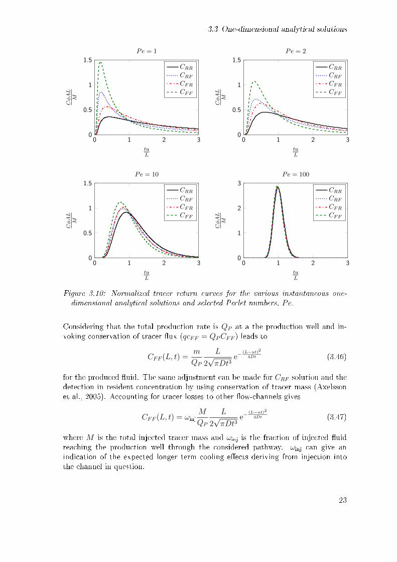
3.10 Normalized tracer return curves for the various instantaneous one-dimensional analytical solutions and selected Peclet numbers, Pe. . . 23
xi

LIST OF FIGURES
3.11 Tracer return curves for the various instantaneous one-dimensionalanalytical solutions and selected Peclet numbers, Pe. The normal-ized concentration is shown on a logarithmic scale to emphasize thedi�erences between the late time predictions of the solutions. . . . . . 24
3.12 Diagram of an idealized single fracture matrix system. . . . . . . . . . 26
4.1 Illustration of di�erence between sorption surface area and heat trans-fer surface area at a fracture surface (Reimus et al., 2012, Williamset al., 2013) . . . . . . . . . . . . . . . . . . . . . . . . . . . . . . . . 32
5.1 Typical grid-point cluster for the one-dimensional problem. . . . . . . 36
5.2 One-dimensional �nite volume grid with N elements. . . . . . . . . . 38
5.3 Control volume for the two-dimensional situation. . . . . . . . . . . . 38
5.4 Control volume within a fracture and neighbouring nodes. . . . . . . 39
6.1 Contours of Rosenbrock's function. . . . . . . . . . . . . . . . . . . . 48
6.2 Tracer pro�les used for testing Algorithms 1 and 2. . . . . . . . . . . 52
7.1 Comparison of �tted one-dimensional instantaneous analytical solu-tions to synthetically generated data using the solution with injectionand detection in �ux concentration. . . . . . . . . . . . . . . . . . . . 57
7.2 Results of �tting a one-dimensional �ux-�ux solution to syntheticdata with Pe = 5 and σnoise = 10%. The upper left plot compares aselected �tted pro�le to the original pro�le with and without noise.The three histograms show the obtained probability density distribu-tions, blue bars, for the �tted parameters. The red curves are theprobability densities assuming Gaussian distributions. . . . . . . . . . 59
7.3 Comparison of one-dimensional numerical and analytical solutionsfor the case of pure advection and continuous injection at constantconcentration, CI . The numerical solution shown used elements ofconstant length ∆x = L/100 and a time step ∆t = ∆x/u. . . . . . . . 60
xii

LIST OF FIGURES
7.4 Comparison of one-dimensional numerical and analytical solutions forthe case of continuous injection at constant �ux concentration, CI ,and detection in �ux, when Pe = 100. The numerical solutions shownemployed constant time steps ∆t = ∆x/u. The lower image showsthe relative di�erence between the numerical and analytical solutions.Grid re�nement clearly improves the numerical solution. . . . . . . . 62
7.5 Comparison of one-dimensional numerical and analytical solutions forthe case of continuous injection at constant �ux concentration, CI ,and detection in �ux, when Pe = 100. The numerical solutions shownused a constant element size of ∆x = L/50. The lower image showsthe relative di�erence between the numerical and analytical solutions. 63
7.6 Comparison of one-dimensional numerical and analytical solutions forthe case of continuous injection at constant �ux concentration, CI ,and detection in �ux, when Pe = 100. The numerical solutions shownused a constant element size of ∆x = L/100 and ∆t = ∆x/u. Thelower graph shows the relative di�erence between the numerical andanalytical solutions. . . . . . . . . . . . . . . . . . . . . . . . . . . . 65
7.7 Comparison of one-dimensional numerical and analytical solutions forthe case of continuous injection at constant �ux concentration, CI ,and detection in �ux, when Pe = 100. The numerical solutions shownused a constant element size of ∆x = L/100 and ∆t = ∆x/u. Thelower image shows the relative di�erence between the numerical andanalytical solutions. . . . . . . . . . . . . . . . . . . . . . . . . . . . 66
7.8 Improper and proper adjustment to account for numerical di�usion,considering numerical di�usion. When calculating the outward �uxD should be used instead of D −Dnum. . . . . . . . . . . . . . . . . . 67
7.9 E�ect of the downstream boundary location for the case of instanta-neous injection and detection in �ux concentration. Lend is the dis-tance of the downstream boundary from the injection well. ∆x = L/103. 68
7.10 Numerical and analytical solutions of the recirculation problem, fordi�erent recirculation fractions, ωinj · ωreinj. The numerical code used∆x = L/103. . . . . . . . . . . . . . . . . . . . . . . . . . . . . . . . . 70
7.11 Comparison of analytical and numerical solutions for injection of a�nite slug in �ux concentration into a one-dimensional �ow-channel.The solutions used a decay rate λ = 2u/L and ∆x = L/500. Thefactor R is a retardation factor describing sorption. . . . . . . . . . . 72
xiii

LIST OF FIGURES
7.12 Numerical results compared with the analytical solution (black curve)for one-dimensional di�usion with a constant concentration boundary,equation (7.22). The numerical solutions shown used equally spacedelements with ∆y = 0.1 m (red circles) and ∆y = 0.05 m (bluetriangles). . . . . . . . . . . . . . . . . . . . . . . . . . . . . . . . . . 74
7.13 Di�erence between the analytical solution of the one-dimensional dif-fusion problem and numerical solutions, for di�erent numbers of el-ements and time steps, ∆t. The solution using 41 elements used∆y = 0.1 m but the one using 81 elements had elements half that size. 75
7.14 Results of modelling one-dimensional matrix di�usion. The resultsillustrate how a variable grid can improve modelling results. . . . . . 76
7.15 Comparison of analytical, CAN , and numerical solutions of the frac-ture matrix model with instantaneous injection in �ux and detectionin �ux. The results show that the variable matrix is more accurate. . 78
8.1 Illustration of the Soda Lake tracer test (Williams et al., 2013). . . . 79
8.2 Measured tracer concentrations at well 32-33 following injection inwell 45A-33 at Soda Lake. The Safranin-T concentrations were cor-rected for thermal decay assuming an e�ective reservoir temperatureof 180◦C. . . . . . . . . . . . . . . . . . . . . . . . . . . . . . . . . . . 81
8.3 Illustration of the di�erence between including and not including re-circulation in the one-dimensional model for the Soda Lake tracertest. A result of using a fairly large but unrealistic delay time for therecirculation is shown to make the di�erence more apparent. . . . . . 84
8.4 Fitted 1,6-NDS tracer pro�le using a realistic 10 hour delay time alongwith the same model without the e�ects of recirculation. . . . . . . . 85
8.5 Fitted Soda Lake tracer data using the one-dimensional version ofthe numerical �nite volume code, assuming a likely delay time forrecirculation. The red dashed line is a numeric �t to the correctedSaf-T data assuming a 180◦C e�ective temperature. . . . . . . . . . . 86
8.6 Matches of Soda Lake tracer data using the one-dimensional versionof the numerical �nite volume code and concurrent �tting of the NDSand uncorrected Saf-T data. The models used a 10 hr delay time forrecirculation and the decay rate for Saf-T was adjustable. . . . . . . . 87
xiv
LIST OF FIGURES
8.7 Matches of Soda Lake tracer data using the one-dimensional versionof the numerical �nite volume code and simultaneous �tting of theearly 1,6-NDS data and all of the uncorrected Saf-T data. The modelsused a 10 hr delay time for recirculation and the decay rate for Saf-Twas adjustable. . . . . . . . . . . . . . . . . . . . . . . . . . . . . . . 89
8.8 Comparison of matched pro�les using single- and double-porositymodels to �t the 1,6-NDS tracer data using the numerical �nite vol-ume code. The models used a 10 hr delay time. . . . . . . . . . . . . 90
9.1 Location of the Laugaland low-temperature geothermal area. Alsoshown are other production areas of Nordurorka (formerly HVA),hot water and return water transmission pipelines, main observationwells, and the microseismic network set up for the 1997-99 reinjectionproject (Axelsson et al., 2001). . . . . . . . . . . . . . . . . . . . . . . 92
9.2 Wells in use in the Laugaland �eld (Axelsson et al., 2001). . . . . . . 94
9.3 Measured �uorescein recovery in well LN-12. . . . . . . . . . . . . . 95
9.4 Observed and simulated �uorescein recovery in well LN-12 during the�rst tracer test. Reinjection into well LJ-08 and production from wellLN-12 (Axelsson et al., 2001). . . . . . . . . . . . . . . . . . . . . . . 97
9.5 Measured and simulated �uorescein recovery in well LN-12 during the�rst tracer test (Liu, 1999). . . . . . . . . . . . . . . . . . . . . . . . 98
9.6 Measured and revised simulations of the �uorescein recovery in wellLN-12 during the �rst tracer test. . . . . . . . . . . . . . . . . . . . . 100
9.7 Measured and �tted simulations of the �uorescein recovery in wellLN-12 during the third tracer test at Laugaland. . . . . . . . . . . . . 101
9.8 Measured �uid temperatures of the production wells at the Laugalandgeothermal �eld (Gautason et al., 2012) . . . . . . . . . . . . . . . . . 103
9.9 Observed temperature at well LN-12 (Gautason et al., 2012). . . . . . 104
9.10 Predicted temperature decline at well LN-12 assuming φf = 1 andD = 0. Zero time is set to coincide with the initiation of reinjection. . 106
9.11 Predicted temperature decline at well LN-12 assuming φf = 0.07 andD = 0. Zero time is set to coincide with the initiation of reinjection. . 106
xv
LIST OF FIGURES
9.12 Predicted temperature decline at well LN-12 assuming φf = 0.07 andD = αu. Zero time is set to coincide with the initiation of reinjection. 108
9.13 Predicted temperature changes at well LN-12 using variable annualinjection and production �ow rates. Zero time is set to coincide withthe initiation of reinjection. . . . . . . . . . . . . . . . . . . . . . . . 108
9.14 Injection and production rates used for the simulated temperaturesshown in Figure 9.13. . . . . . . . . . . . . . . . . . . . . . . . . . . . 109
9.15 Predicted temperature decline at well LN-12 within the Laugalandgeothermal �eld, assuming an average 20 L/s production rate at wellLN-12 and a 10 L/s injection rate at well LJ-08. Zero time is set tocoincide with the initiation of reinjection in 1997. . . . . . . . . . . . 110
xvi

List of Tables
3.1 Solutions to the one-dimensional advection-dispersion equation forinstantaneous injection of tracer mass m into a �ow-channel with across-sectional area A, porosity φ and a �ow rate q = φAu (Kreft andZuber, 1978). . . . . . . . . . . . . . . . . . . . . . . . . . . . . . . . 21
3.2 Solutions to the one-dimensional advection-dispersion equation forcontinuous injection (Kreft and Zuber, 1978). . . . . . . . . . . . . . 22
6.1 Performance of optimization algorithms for solving the Rosenbrockproblem. . . . . . . . . . . . . . . . . . . . . . . . . . . . . . . . . . . 49
6.2 Values used for Meyer's problem. . . . . . . . . . . . . . . . . . . . . 50
6.3 Performance of optimization algorithms for solving the Meyer problem. 50
6.4 Performance of optimization algorithms for solving the scaled Meyerproblem. . . . . . . . . . . . . . . . . . . . . . . . . . . . . . . . . . . 51
6.5 Performance of optimization algorithms when �tting one tracer peak,with τ = 1 and M = 100 kg. . . . . . . . . . . . . . . . . . . . . . . . 53
6.6 Performance of optimization algorithms when �tting one tracer peak,with τ = 1 · 10−6 and M = 100 kg. . . . . . . . . . . . . . . . . . . . 53
6.7 Performance of optimization algorithms when �tting one tracer peak,with scaled �tting parameters and τ = 1 · 100. . . . . . . . . . . . . . 54
6.8 Performance of optimization algorithms when �tting one tracer peak,with scaled �tting parameters and τ = 1 · 10−6. . . . . . . . . . . . . 54
7.1 Results of �tting one-dimensional models to synthetic CFF data. . . . 56
xvii

LIST OF TABLES
7.2 Results of �tting one-dimensional CFF model to synthetic CFF datawith noise. . . . . . . . . . . . . . . . . . . . . . . . . . . . . . . . . . 58
8.1 Best �tting RELAP parameters, for the Soda Lake tracer experiment,for di�erent conceptual models (Williams et al., 2013). . . . . . . . . 82
8.2 Results using the single-porosity numerical �nite volume method tomatch the Soda Lake data, for di�erent delays in recirculation. Hereit was assumed that the 1,6-NDS tracer was injected during the �rsthalf hour and the Saf-T tracer was injected over the following threehours. . . . . . . . . . . . . . . . . . . . . . . . . . . . . . . . . . . . 83
9.1 Summary of the tracer experiment conducted at Laugland from Septem-ber 1997 to August 1999 and some results (Axelsson et al., 2001). . . 93
9.2 Previous results from interpreting the �rst tracer test at Laugaland.The tracer returns at well LN-12 were interpreted using the instanta-neous, one-dimensional CRR solution and assuming three �ow-paths.The dispersion coe�cients is assumed to be D = αu. . . . . . . . . . 96
9.3 Revised interpretation of the �rst tracer test at Laugaland, usingvarious one-dimensional (linear) solutions with instantaneous tracerinjection. The dispersion coe�cients is assumed to be D = αu. . . . . 99
9.4 Initial interpretation of the third tracer test at Laugaland, using theinstantaneous solutions which have detection in �ux concentration.The dispersion coe�cients is assumed to be D = αu. . . . . . . . . . 101
xviii

Nomenclature
A Cross-sectional area of �ow-channel [m2]
b Fracture half aperture [m]
b−1 Surface area to volume ratio [m−1]
ci Speci�c heat capacity of material i [J/g◦C]
C Solute concentration [kg/m3]
CF Flux concentration [kg/m3]
CI Injection concentration [kg/m3]
CP Production concentration [kg/m3]
CR Resident concentration [kg/m3]
Cr Courant number [-]
D Hydraulic dispersion coe�cient [m2/s]
De� E�ective molecular di�usion coe�cient [m2/s]nomeqref 3.9
Dmech Mechanical dispersion coe�cient [m2/s]nomeqref 3.4
Dmol (Apparent) molecular di�usion coe�cient [m2/s]nomeqref 3.4
Dr Radial dispersion coe�cient [m2/s]nomeqref 3.42
Ff Formation factor [-]
G Approximation of the Jacobian matrix
J Jacobian matrix
k A mass based sorption partition coe�cient [m3/kg]
xix

LIST OF TABLES
kth Thermal conductivity [W/(m·K)]
Ka A surface-area-based sorption partition coe�cient [m3/m2]
L Length of �ow-channel [m]
m Tracer mass in a given �ow-channel [kg]
M Total injected tracer mass [kg]
Pe Peclet number [-]
q Flow-channel �ow rate [m3/s]
Q Flow rate [m3/s]
QI Injection rate [m3/s]
QP Production rate [m3/s]
r Radial coordinate [m]
r Residual vector
Rf Fracture retardation factor [-]
Rm Matrix retardation factor [-]
S Tracer surface concentration on the solid rock phase [kg/kg]
t Time [s]
td Pipeline delay time [s]
T Temperature [K] or [◦C]
T0 Initial formation temperature [K] or [◦C]
TI Temperature of injected �uid [K] or [◦C]
TP Temperature of produced �uid [K] or [◦C]
u Average linear velocity [m/s]
ur Radial velocity [m/s]
x Distance along the �ow-path [m]
y Distance from the fracture centerline [m]
z Vector of unknown model parameters
xx

LIST OF TABLES
α Dispersivity [m]
δ Constrictivity [-]
κ Thermal di�usivity [m2/s]
λ Decay rate [s−1]
λf Decay rate in the �uid phase [s−1]
λs Decay rate in the solid phase [s−1]
ρi Density of material i [kg/m3]
ρR Rock density [kg/m3]
ρw Fluid density [kg/m3]
τ Tortuosity [-]
τf Tortuosity factor [-]
φ Porosity [-]
φf Fracture porosity [-]
φm Matrix porosity [-]
ωinj Fraction of injected �uid reaching the production well
ωreinj Fraction of injection �uid deriving from the production �uid
xxi

Acknowledgments
I am indebted to my supervisor Dr. Guðni Axelsson for his invaluable supportand guidance during my masters study. Dr. Sigrún Hreinsdóttir acted as facultysupervisor and was always available to give me good advice, for which I am grateful.I also thank Dr. Egill Júlíusson for his constructive criticism. I appreciate theinput of Dr. Peter Rose (University of Utah) and Dr. Paul Reimus (Los AlamosNational Laboratory) who supplied the Soda Lake data and discussed its modelling.My thanks go to Iceland Geosurvey (ÍSOR) for the data from Laugaland and forproviding a place for me to work on this dissertation. I am very thankful for theenthusiastic advice of Dr. Sven Þ. Sigurðsson on aspects of numerical modelling. Dr.Stefan Finsterle and Dr. Christine Doughty were kind enough to listen to my ideasand encourage me when I met them at Lawrence Berkeley National Laboratory.This research was supported by a grant from Landsvirkjun, and Stapi ConsultingGeologists provided �nancial assistance. I am grateful for their contributions. Lastbut not least, I thank my family and friends who have helped and supported meduring my studies.
xxiii

1 Introduction
Reinjection is an important aspect of geothermal utilisation. Originally reinjectionwas simply used as a means to dispose of waste water. Later it was realised that ifperformed correctly it can increase long term energy extraction and the longevityof a geothermal �eld (Axelsson, 2008, Stefansson, 1997). Reinjecting spent �uido�ers supplementary recharge to the system and helps limit pressure decline. Inaddition to improving resource recovery, injection can be of bene�t for places that areprone to subsidence (Axelsson, Kaya et al., 2011, Stefansson, 1997) and can be usedto reinvigorate natural geothermal surface features impacted by over-production(Bromley et al., 2006).
Suitable reinjection strategies depend on the system type and location of wells. Forvapour-dominated systems, which by their nature are lacking in natural recharge,reinjection should be in�eld. Whereas for hot-water and two-phase, liquid-dominatedsystems the approach may involve some combination of in�eld and out�eld injec-tion. One of the main issues with injecting cool �uid into a geothermal system is thepossibility of thermal breakthrough. Undesirable thermal changes can be avoidedby siting injection wells far enough away from the production zone. The oppositearrangement is desirable to stave o� pressure decline. A balance needs to be struckbetween the gain in pressure from in�eld injection and possible lowering of the rateof energy extraction because of the advancement of cool reinjection �uid throughthe �eld (Kaya et al., 2011, Mannington et al., 2004).
Tracer testing can provide insights into aspects of groundwater �ow which are notprovided by other reservoir examination methods. The aim of this study was toreview existing methods for interpreting tracer experiments and to develop traceranalysis methods for thermal breakthrough forecasting and apply them to selectedcase histories. This study used both analytical and numerical methods to interprettracer return pro�les to predict thermal breakthrough induced by reinjection intogeothermal reservoirs. Tracer tests can give qualitative results regarding �ow-pathsbut this work was concerned with the quantitative interpretation of tracer data.
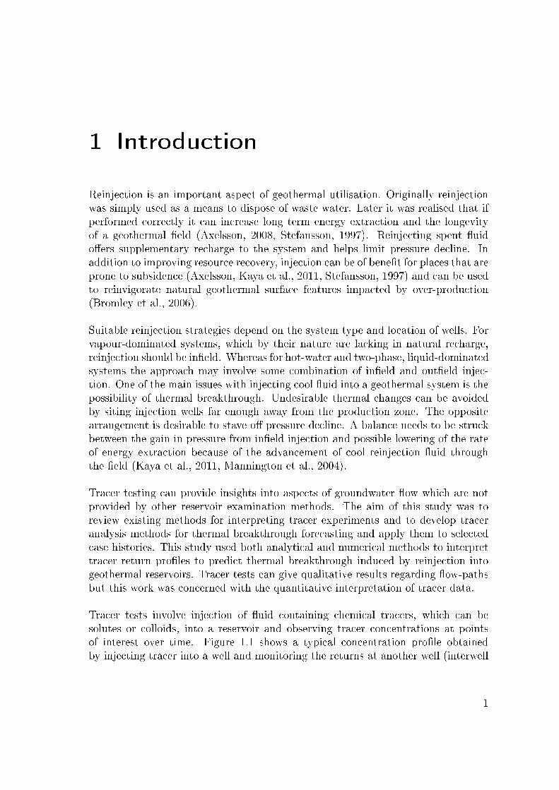
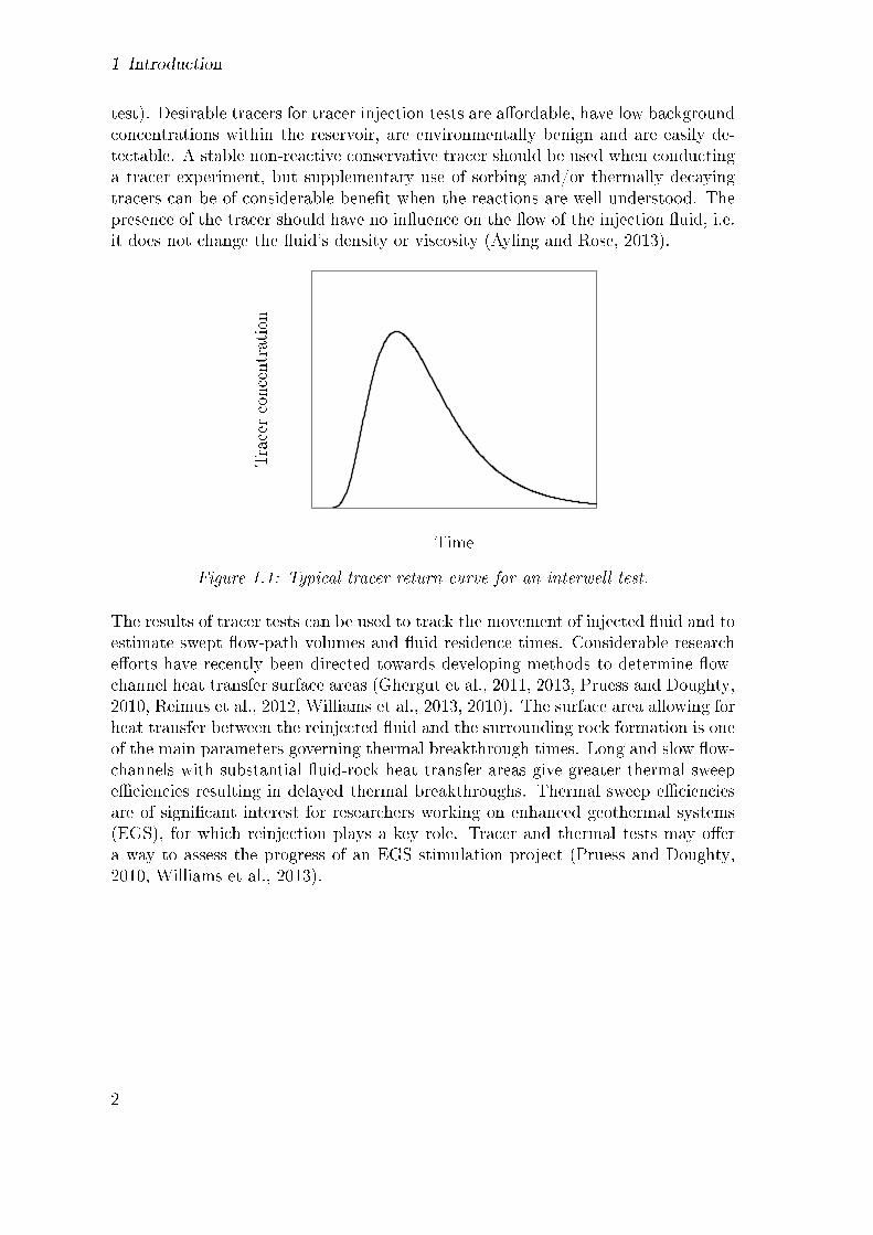
Tracer tests involve injection of �uid containing chemical tracers, which can besolutes or colloids, into a reservoir and observing tracer concentrations at pointsof interest over time. Figure 1.1 shows a typical concentration pro�le obtainedby injecting tracer into a well and monitoring the returns at another well (interwell
1
1 Introduction
test). Desirable tracers for tracer injection tests are a�ordable, have low backgroundconcentrations within the reservoir, are environmentally benign and are easily de-tectable. A stable non-reactive conservative tracer should be used when conductinga tracer experiment, but supplementary use of sorbing and/or thermally decayingtracers can be of considerable bene�t when the reactions are well understood. Thepresence of the tracer should have no in�uence on the �ow of the injection �uid, i.e.it does not change the �uid's density or viscosity (Ayling and Rose, 2013).
Time
Tracerconcentration
Figure 1.1: Typical tracer return curve for an interwell test.
The results of tracer tests can be used to track the movement of injected �uid and toestimate swept �ow-path volumes and �uid residence times. Considerable researche�orts have recently been directed towards developing methods to determine �ow-channel heat transfer surface areas (Ghergut et al., 2011, 2013, Pruess and Doughty,2010, Reimus et al., 2012, Williams et al., 2013, 2010). The surface area allowing forheat transfer between the reinjected �uid and the surrounding rock formation is oneof the main parameters governing thermal breakthrough times. Long and slow �ow-channels with substantial �uid-rock heat transfer areas give greater thermal sweepe�ciencies resulting in delayed thermal breakthroughs. Thermal sweep e�cienciesare of signi�cant interest for researchers working on enhanced geothermal systems(EGS), for which reinjection plays a key role. Tracer and thermal tests may o�era way to assess the progress of an EGS stimulation project (Pruess and Doughty,2010, Williams et al., 2013).
2
2 Literature review
Tracer tests are regularly used to assess groundwater �ow through various forma-tions. Research into the dispersal of contaminants from nuclear waste disposal siteshas contributed greatly to development in the �eld of tracer testing. Methods usedto determine tracer �ow characteristics in geothermal reservoirs draw on experiencefrom such works and similar endeavours in the �eld of petroleum engineering.
The possibility of thermal breakthrough has been understood since early in the his-tory of geothermal utilisation. By virtue of the highly fractured nature of mostgeothermal reservoirs, injection �uid may easily �nd its way through a permeablenetwork of �ssures connecting injection and production wells. In 1981 Nakamura re-ported complications in production due to reinjection of spent water in Japan. Horne(1982) summarized experiences gained with reinjection around this time; researchindicated a relationship between tracer return times and thermal breakthrough.Stefansson (1997) reported that in some cases change in production enthalpy fromhigh temperature systems is interpreted as thermal breakthrough, when it is morelikely that the di�erence in enthalpy results from pressure changes in a two-phasereservoir. According to Stefansson (1997), cooling as a result of reinjection had, atthe time of writing, only been con�rmed for Ahuachapán (El Salvador), Palinpinon(Philippines) and Svartsengi (Iceland).
Horne and Rodriguez (1981) developed mathematical descriptions of tracer �ow inan idealized fracture undergoing purely convective-dispersion and Taylor dispersion.For the case of convective-dispersion they assumed that the �ow could be describedby one-dimensional channel �ow. Neglecting molecular di�usion in the �ssure leadsto macroscopic dispersion since the �uid's velocity is not constant across the widthof the fracture. Allowing for transverse molecular di�usion of the tracer, Horne andRodriguez (1981) found a simple mathematical relation for the e�ective longitudinaldispersivity in terms of the fracture aperture, the �uid average velocity and themolecular di�usivity. Fossum and Horne (1982) used a one-dimensional model, basedon the work of Horne and Rodriguez (1981), to match tracer pro�les from interwelltracer experiments performed in the Wairakei geothermal �eld, New Zealand. Theywere unable to get a satisfactory �t using only one �ow-path but a closer �t couldbe attained assuming two �ow-paths (Horne et al., 1982).
Further tests on the Wairakei �eld indicated that this model did not fully account
3
2 Literature review
for the processes governing the �ow in the Wairakei system. Jensen and Horne(1983) obtained an improved �t to the Wairakei data using a dual-porosity model.Their model allows for tracer di�usion between the fracture and the surroundingrock matrix as well as tracer sorption onto the rock. The model was developed byNeretnieks et al. (1982) for studying transfer of radionuclides in a natural �ssure in agranite core. A compact analytical solution was obtained for the model since neitherdispersion nor matrix di�usion parallel to the fracture was taken into account.
Bullivant and O'Sullivan (1985) presented the results of applying a uniform porousmodel, a pseudo-steady state double porosity model and the fracture-matrix modelused by Jensen and Horne (1983) to the Wairakei tracer data. Their results were sim-ilar to those of Fossum and Horne (1982) and Jensen and Horne (1983). This is notsurprising considering the uniform porous model used by Bullivant and O'Sullivan(1985) is mathematically equivalent to the one employed by Fossum and Horne(1982), apart from the formulation of the injection conditions. However, the pseudo-steady state double porosity model did not improve upon the results found by usingthe uniform porous model.
Kocabas and Horne (1987) suggested using single-well injection-withdrawal tracertests for characterizing �ow in fractured geothermal systems. They advocated usingsingle-well tests prior to applying interwell investigations. Their reasoning is thatsingle-well experiments require less time than the interwell ones. Moreover, accord-ing to Kocabas and Horne (1987) injection-back�ow tests have the possibility of sup-plying the same amount of information as the interwell tracer tests. In their study,Kocabas and Horne (1987) e�ectively used the same conceptual models as Fossumand Horne (1982) and Jensen and Horne (1983) with the added complexity of havingto solve for the additional back�ow period. Kocabas and Horne (1987) applied theiranalytical solutions to tracer test data from Raft River and East Mesa geothermal�elds, USA. Their results are similar to those of Fossum and Horne (1982) andJensen and Horne (1983), with the use of a matrix di�usion model giving the morereasonable matches to the data. The data �ts using the convective-dispersion modelworsen for increasing injection times. Kocabas and Horne (1987) attributed this tothe e�ects of the fracture-matrix interaction becoming more pronounced with time.
Kocabas and Horne (1990) developed the idea of using single-well tests further.In their paper from 1990 they proposed adopting thermal injection-back�ow testsalong with interwell tracer tests to predict thermal breakthrough. More recent pa-pers dealing with the issues pertaining to thermal injection-back�ow tests are: Jungand Pruess (2012), Kocabas (2005, 2010), Maier and Kocabas (2013b), Pruess andDoughty (2010). Pruess and Doughty (2010) conducted numerical simulation ex-periments for single-well injection-back�ow tests. Their preliminary results showedthat temperature returns are sensitive to heat transfer area while being insensitiveto changes in fracture aperture and porosity. Using an analytical solution, Jungand Pruess (2012) also found indications that the fracture aperture a�ects thermal
4
recovery faintly for injection back�ow tests.
Shook (2001) suggested a novel and rather simple method for thermal breakthroughprediction. Shook's approach used the equivalence of the mathematical equationsdescribing the transport of tracers and thermal fronts for one-dimensional �ow inporous media. By neglecting conduction as a second order e�ect a predicted thermaldecline can be found with an integral transform of the tracer data.
The tracer transport models mentioned thus far have mostly assumed that the dis-persive mechanism is either matrix di�usion or convective-dispersion, but not both.There are mainly two reasons for this. First of all, simple analytical solutions aremore easily obtained assuming dispersion/di�usion in only one of the spatial dimen-sions. Furthermore, since di�usion and dispersion are similar processes it is di�cultto discern the di�erence between them in tracer data. The use of multiple tracerswith varying properties has been suggested to solve this problem. Results of ex-periments performed by Maloszewski et al. (1999) in fractured rocks show that aminimum of two tracers with distinct coe�cients of molecular di�usion is needed toachieve valid conclusions. Maloszewski et al. (1999) pointed out that at least one ofthe tracers used should be conservative to di�erentiate the e�ects of di�usion andsorption.
Reimus and Haga (1999) developed software code that uses a semi-analytical dual-porosity transport model called RELAP (REactive transport LAPlace transforminversion code) to interpret interwell tracer tests. RELAP gives an option of usingeither a linear or radial dual-porosity model. The dual-porosity model consists ofone-dimensional advective-dispersive fracture �ow with matrix di�usion and includestracer sorption. The inversion code within RELAP is capable of �tting up to fourtracer pro�les together to attain consistent parameter estimations.
Recent studies have looked at new types of tracers to characterize �ow in geothermalsystems. Becker et al. (2013), Dean et al. (2013, 2012), Sullivan et al. (2003),Williams et al. (2013, 2010) have conducted �eld, lab and numerical experiments onthe use of cation exchange tracers to assess matrix di�usion and �ow-path surfaceareas. Advances in tracer technology such as thermosensitive tracers (Ames et al.,2013, Williams et al., 2013) and quantum dots (Rose et al., 2011) have the potentialto improve �ow-path interrogation and thermal breakthrough forecasting. Injectionof conductive �uid and measurement of the resulting change in electrical potentialis another possible tool for characterizing reservoir connectivity (Magnusdottir andHorne, 2013).
Numerous articles have been published describing methods to match tracer returns,as well as some papers developing methods which use results of tracer tests to predictthermal changes in reservoirs. Yet there is a limited amount of published researchwhere these methods have been applied to forecast thermal breakthroughs in actual
5
2 Literature review
geothermal systems. Malate and O'Sullivan (1991) used a fracture �ow model cou-pled with a lumped mass balance model to match thermal drawdown in well PN-26,Palinpinon geothermal �eld, Philippines. Cooling of about 50◦C was observed inwell PN-26 over three years. The lumped parameter model accounts for observedchloride changes which occurred as a result of reinjection. The model gave a goodmatch to the temperature history. Results of tracer tests have been used to predictcooling of produced �uids resulting from reinjection in N-Iceland (Axelsson et al.,1995, 2001). Axelsson et al. (1995) and Axelsson et al. (2001) used a one-dimensionaldispersive channel-�ow model like Fossum and Horne (1982) for history matchingof tracer responses. The results of the tracer tests were extended to a fracture-zonemodel to infer long term thermal changes for various reinjection scenarios with con-stant �ow rates. Maturgo et al. (2010) used the same software package, ICEBOX(Arason et al., 2003), as Axelsson et al. (1995, 2001) to forecast thermal cooling inthe Southern Negros geothermal �eld, Philippines, using tracer data. Co (2012), andCo and Horne (2012) used a coupled tracer and temperature model for concurrent�tting of tracer and temperature data from the Southern Negros geothermal �eldand the Hijiori EGS test site, Japan. Co (2012), Co and Horne (2012) used thesame one-dimensional uniform porous model as Bullivant and O'Sullivan (1985) forthe tracer data and the same type of temperature model as Axelsson et al. (1995,2001), and Maturgo et al. (2010). Co (2012) compared her results to the modellingdone by Maturgo et al. (2010).
Axelsson et al. (1995, 2001) used their thermal predictions to evaluate possibleincreases of energy production stemming from reinjection. Juliusson (2012) andJuliusson and Horne (2013) developed a method which uses thermal predictionsfound by interpreting �ow rate and tracer data for production management. Intheir study they created arti�cial tracer data using a reservoir simulator. They useda method formulated by Juliusson to match tracer returns under variable �ow-ratesin fractured geothermal systems. Juliusson (2012), Juliusson and Horne (2013)set up an optimization problem with an objective function which maximizes thepro�tability of production from the geothermal �eld with respect to injection rates.Such a method could be used to predict the most favourable injection-productionscenarios.
The next chapter discusses tracer test theory in more detail, including the relevantpublished studies and solutions used to match tracer breakthroughs.
6
3 Tracer test theory
Selecting a suitable model to describe subsurface �ow in a geothermal system is anontrivial task. For the case of describing tracer transport multiple aspects have tobe considered. Having some insight into the geological structure of the system willassist with selecting a possible model. The scale of the test area with respect to the�ow network may in�uence which model is adopted. Over a small range the �owmay be dominated by one fracture and a single �ow-path model can be appropriate.Other areas will be more complex with multiple pathways. Those �elds can call forgreater sophistication in the modelling. However, the simplest model that solves theproblem adequately will likely be the most practical. On very large scales a singleporous medium approach is often used e�ectively to describe geothermal systems(O'Sullivan et al., 2001). The phase of the geothermal �uid is another factor thatwill a�ect the choice of a suitable model. A two phase system can require a morecomplex model that includes tracer migration between the liquid and vapour phasesof the �uid. Depending on the solute used for a given tracer test the model mayalso have to account for chemical processes that can in�uence the tracer returns.These processes include tracer degradation and sorption. Last, but not least, theinjection and detection modes establish the initial and boundary conditions for themodel. Bodin et al. (2003) give a good summary of mechanisms in�uencing tracertransport within fractured aquifers.
Phase partitioning tracers can be used to estimate phase partitioning within two-phase reservoirs. This work is limited to a discussion on tracer migration withina single-phase geothermal liquid. For those interested in the subject of boiling ofinjection �uid, Pruess (2002), Pruess et al. (2000), Trew et al. (2000) and Wu et al.(2008) give a good overview of processes controlling phase partioning in geothermalreservoirs and discuss ways of modelling tracer transport under two-phase conditions.The underlying fundamentals are the same as for the single-phase case but with theadded intricacy of having to account for interplay of the di�erent phases.
In this study, interwell tracer tests are considered for predicting thermal break-through in production wells caused by reinjection. Interwell methods are preferableto the single-well tests since they measure the relationship between the injection andproduction wells. Single-well tests have the drawback of measuring the �ow only inthe close vicinity of the injection well. The �ow around the injection well does notnecessarily represent the �ow characteristics between the injection and production
7
3 Tracer test theory
wells. The dominant �ow-paths around the injection well may not be connectedwith the production well.
Thermal injection-back�ow tests seem appealing because they measure thermalchange, the main process of interest. Moreover, thermal di�usivities of rocks areabout four orders of magnitude greater than e�ective rock-matrix di�usion coe�-cients for tracers. The fracture-matrix interaction will accordingly be greater forthermal transport than in the case of tracer migration. The disadvantage of usingthermal-injection tests is the slow movement of thermal fronts compared with so-lute advances. Transport of thermal fronts along main �ow-paths such as fracturesare impeded by the thermal di�usion into the surrounding rock. The single wellthermal injection back�ow method therefore has the additional drawback of havinga very short measurement range compared to injection back�ow tests conductedusing chemical tracers. The predictive power of interwell tracer tests is due to thefaster transport of tracers compared to thermal fronts along �ow-channels (Axelsson,2013).
3.1 The advection-dispersion equation
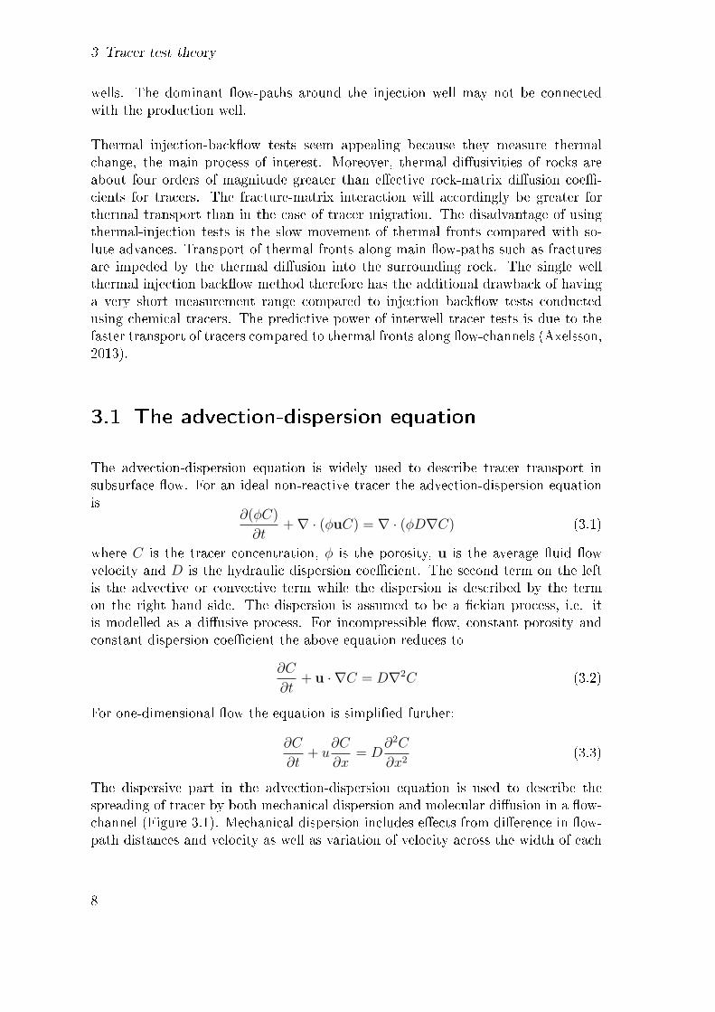
The advection-dispersion equation is widely used to describe tracer transport insubsurface �ow. For an ideal non-reactive tracer the advection-dispersion equationis
∂(φC)
∂t+∇ · (φuC) = ∇ · (φD∇C) (3.1)
where C is the tracer concentration, φ is the porosity, u is the average �uid �owvelocity and D is the hydraulic dispersion coe�cient. The second term on the leftis the advective or convective term while the dispersion is described by the termon the right hand side. The dispersion is assumed to be a �ckian process, i.e. itis modelled as a di�usive process. For incompressible �ow, constant porosity andconstant dispersion coe�cient the above equation reduces to
∂C
∂t+ u · ∇C = D∇2C (3.2)
For one-dimensional �ow the equation is simpli�ed further:
∂C
∂t+ u
∂C
∂x= D
∂2C
∂x2(3.3)
The dispersive part in the advection-dispersion equation is used to describe thespreading of tracer by both mechanical dispersion and molecular di�usion in a �ow-channel (Figure 3.1). Mechanical dispersion includes e�ects from di�erence in �ow-path distances and velocity as well as variation of velocity across the width of each
8

3.1 The advection-dispersion equation
Velocitypro�le
Grain
(a) (b)
Grain
(c)
Figure 3.1: Dispersion due to mechanical spreading (a,b), and molecular di�usion(c). Modi�ed from Bear and Cheng (2010).
�ow-channel. Part of the dispersion can be explained by tortuous routes between therock grains and within the pores of the rock, while on a larger scale dispersion occursbecause of variation of permeability and length of major �ow-paths (Figure 3.2).Mathematically the hydraulic dispersion coe�cient is a combination of mechanicaldispersion (Dmech) and molecular di�usion (Dmol):
D = Dmech +Dmol (3.4)
It is a di�cult task, in practice, to discern the di�erence between di�usive anddispersive processes a�ecting tracer returns. Nevertheless, molecular di�usion isinconsequential compared to dispersion along advection dominated �ow-paths. Thisis likely the case for �ow along fractures within geothermal �elds. Di�usion canplay an important role in solute migration into stagnant �uid and fracture-matrixinteraction (Maloszewski et al., 1999, Pruess et al., 2000).
The mechanical dispersion is often assumed to be linearly related the average �owvelocity according to
Dmech = αu (3.5)
Figure 3.2: Idealized diagram of a fracture network.
9

3 Tracer test theory
where α is the dispersivity. This can be given more generally by
Dmech = αun (3.6)
where n is some value that needs to be determined empirically (Freeze and Cherry,1979). The dispersivity is in many applications considered constant. The dispersiv-ity will vary depending on the degree of heterogeneity within the �eld and the scaleof the test area (Gelhar et al., 1992).
For one-dimensional tracer migration by di�usion in saturated porous media thetransport equation is given by
φ∂C
∂t= De�
∂2C
∂x2(3.7)
The e�ective di�usion coe�cient, De�, is related to the apparent di�usion coe�cientDmol as follows:
De� = φDmol (3.8)
The e�ective di�usivity will largely depend on features of the porous medium, pore�uid and the di�using tracer species (Pruess, 2002). In the above equation and pre-vious ones it is assumed that for tracer �uxes the "surface porosity" of the medium isequal to its porosity. The surface porosity is de�ned as the ratio of void area to totalarea for a given cross section of the porous medium, while the porosity is the fractionof void volume over the total volume. Strictly speaking, φ is the e�ective porositysince some of the voids are unavailable for transport (Nield and Bejan, 2006). Someauthors use more complicated equations to describe the e�ective di�usion (Bovingand Grathwohl, 2001, Neretnieks, 1980):
De� =φ
τ 2D∗mol =
φ
τfD∗mol (3.9)
Here τ is the tortuosity, τf the tortuosity factor and D∗mol is the molecular di�usioncoe�cient for free di�usion in water. The tortuosity is de�ned as the ratio of theaverage or e�ective path length, le, to the straight-line distance between the ends ofthe �ow-path, l, see Figure 3.3. It is evident from this de�nition and Figure 3.3 thatτ ≥ 1. Equation (3.9) is based on a porous medium model where the pores consistof a bunch of parallel sinusoidal capillaries (Grathwohl, 1998a). Equation (3.9) issometimes presented with an added multiplication factor, δ ≤ 1, called the con-strictivity (Boving and Grathwohl, 2001, Maloszewski and Zuber, 1990, Neretnieks,1980):
De� =φ δ
τ 2D∗mol =
φ δ
τfD∗mol (3.10)
The constrictivity becomes important when the size of the solute is comparable tothe pore size (Boving and Grathwohl, 2001). An empirical relation, analogous to
10

3.1 The advection-dispersion equation
le
l
Figure 3.3: Tortuous path in a porous medium.
Archie's law for electrical conductivity of porous rocks, is also used to describe thee�ective di�usion (Boving and Grathwohl, 2001, Grathwohl, 1998a,b):
De� = φmD∗mol (3.11)
The most compact way of describing the e�ective di�usion could be to use a singleformation factor:
De� = Ff D∗mol (3.12)
The formation factor, Ff , can be thought of as being some function of the porousmedium's porosity and other possible contributing factors.
The solution of (the one-dimensional advection-dispersion equation (equation 3.7) )
∂C
∂t+ u
∂C
∂x= D
∂2C
∂x2(3.13)
given the initial and boundary conditions
C(x) = δ(x) , t = 0 (3.14)
limx→±∞
C(x, t) = 0 (3.15)
is called the fundamental solution of the advection-di�usion equation. The solutionis
C(x, t) =1
2√πDt
e−(x−ut)2
4Dt (3.16)
By noting that
δ(x) = lima→0
1
a√π
e−x2
a2 (3.17)
andδ(x) = δ(x− ut)|t=0 (3.18)
it is clear that the solution meets the given conditions. The fundamental solution isone of multiple solutions used by researchers to match tracer return pro�les (Axels-son et al., 1995, 2001, Fossum and Horne, 1982). The solution needs to be adjustedto account for the amount of tracer injected (in reality, detected since some of the
11
3 Tracer test theory
tracer may not be recovered). For instantaneous injection of mass M of solute attime t = 0 the initial conditions become:
C(x, 0) =M
φAδ(x) =
Mu
qδ(x) (3.19)
where A is the cross-sectional area of the �ow-path and q is the injection rate. Inthis thesis the average velocity, u, is assumed positive unless otherwise stated. Thesolution, given the initial conditions above, is simply the one given by equation(3.16) multiplied by the appropriate factor:
C(x, t) =M
φA
1
2√πDt
e−(x−ut)2
4Dt =Mu
q
1
2√πDt
e−(x−ut)2
4Dt (3.20)
Numerous other solutions of the advection dispersion equation can be found in theliterature. The solutions depend on the initial and boundary conditions a givenresearcher considers appropriate for the system being described, as reviewed in thefollowing section.
3.2 Boundary and initial conditions
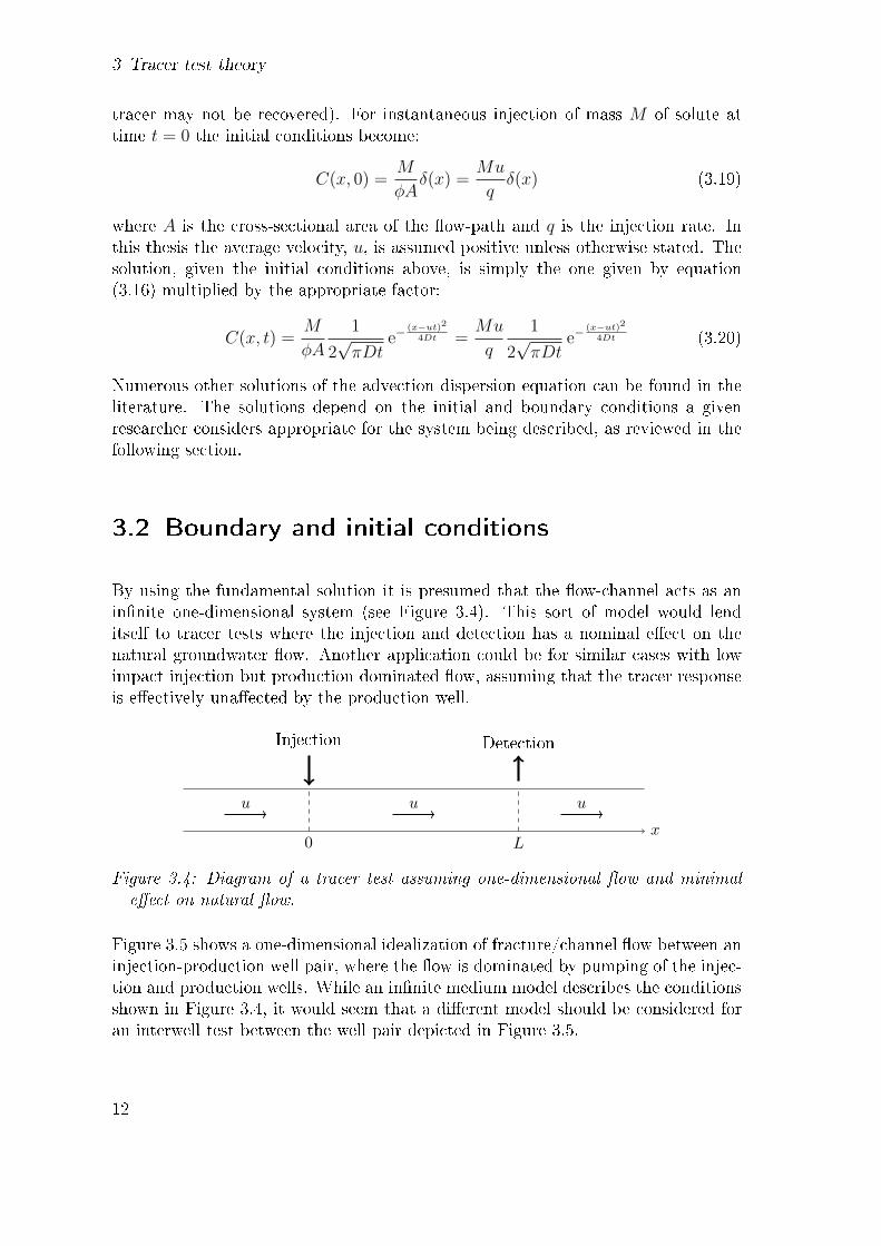
By using the fundamental solution it is presumed that the �ow-channel acts as anin�nite one-dimensional system (see Figure 3.4). This sort of model would lenditself to tracer tests where the injection and detection has a nominal e�ect on thenatural groundwater �ow. Another application could be for similar cases with lowimpact injection but production dominated �ow, assuming that the tracer responseis e�ectively una�ected by the production well.
0 Lx
Injection Detection
u uu
Figure 3.4: Diagram of a tracer test assuming one-dimensional �ow and minimale�ect on natural �ow.
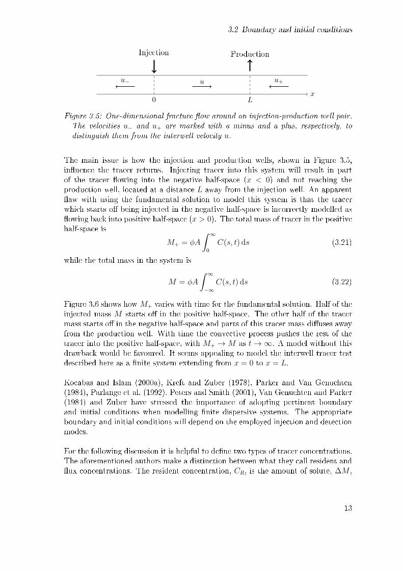
Figure 3.5 shows a one-dimensional idealization of fracture/channel �ow between aninjection-production well pair, where the �ow is dominated by pumping of the injec-tion and production wells. While an in�nite medium model describes the conditionsshown in Figure 3.4, it would seem that a di�erent model should be considered foran interwell test between the well pair depicted in Figure 3.5.
12
3.2 Boundary and initial conditions
0 Lx
Injection Production
u u+u−
Figure 3.5: One-dimensional fracture �ow around an injection-production well pair.The velocities u− and u+ are marked with a minus and a plus, respectively, todistinguish them from the interwell velocity u.
The main issue is how the injection and production wells, shown in Figure 3.5,in�uence the tracer returns. Injecting tracer into this system will result in partof the tracer �owing into the negative half-space (x < 0) and not reaching theproduction well, located at a distance L away from the injection well. An apparent�aw with using the fundamental solution to model this system is that the tracerwhich starts o� being injected in the negative half-space is incorrectly modelled as�owing back into positive half-space (x > 0). The total mass of tracer in the positivehalf-space is
M+ = φA
∫ ∞0
C(s, t) ds (3.21)
while the total mass in the system is
M = φA
∫ ∞−∞
C(s, t) ds (3.22)
Figure 3.6 shows how M+ varies with time for the fundamental solution. Half of theinjected mass M starts o� in the positive half-space. The other half of the tracermass starts o� in the negative half-space and parts of this tracer mass di�uses awayfrom the production well. With time the convective process pushes the rest of thetracer into the positive half-space, with M+ →M as t→∞. A model without thisdrawback would be favoured. It seems appealing to model the interwell tracer testdescribed here as a �nite system extending from x = 0 to x = L.
Kocabas and Islam (2000a), Kreft and Zuber (1978), Parker and Van Genuchten(1984), Parlange et al. (1992), Peters and Smith (2001), Van Genuchten and Parker(1984) and Zuber have stressed the importance of adopting pertinent boundaryand initial conditions when modelling �nite dispersive systems. The appropriateboundary and initial conditions will depend on the employed injection and detectionmodes.
For the following discussion it is helpful to de�ne two types of tracer concentrations.The aforementioned authors make a distinction between what they call resident and�ux concentrations. The resident concentration, CR, is the amount of solute, ∆M ,
13

3 Tracer test theory
0 2 4 6 8 100.5
0.6
0.7
0.8
0.9
1
v2tD
M+
M
Figure 3.6: Time dependence of the total mass within the positive half-space for thefundamental solution.
in a unit volume, ∆V , of �uid at a given time:
CR =∆M
∆V(3.23)
It has been assumed to this point that the concentration, C, in the advection dis-persion equation is the resident concentration. The �ux concentration on the otherhand is the ratio of solute �ux to �uid �ux passing through a given cross section.Seeing as the �uid �ux is equal to the advective �ux:
Φ�uid = φuA (3.24)
and the solute �ux is a combination of the advective and dispersive �ux:
Φsolute = φ
[uCR −D
∂CR∂x
]A (3.25)
then the �ux concentration is
CF =Φsolute
Φ�uid
= CR −D
u
∂CR∂x
(3.26)
It is apparent that the �ux concentration, CF , tends towards the resident concen-tration, CR, as the dispersion becomes more negligible. The two concentrationexpressions become equal in cases where the resident concentration gradient is zeroand/or there is no dispersive/di�usive �ux. It can be easily shown that the �uxconcentration is a solution to equation (3.7) (Kreft and Zuber, 1978). The samecan be shown for the advection-dispersion equation including source terms which
14
3.2 Boundary and initial conditions
are linearly dependent on the resident concentration (Kocabas and Islam, 2000a,Parlange et al., 1992).
Mass conservation leads to the following relation for the �ux and resident concen-trations (Kreft and Zuber, 1978):
q
∫ t
0
CF (x, τ) dτ = φA
∫ ∞x
CR(s, t) ds (3.27)
It states that the net amount of solute that has passed through the cross-sectionat x has to be located between x and ∞. Equation (3.27) assumes that the �ux ispositive and CR(s, 0) = 0, for s > x.
3.2.1 Inlet boundary
It can be intuitively appealing when modelling a �nite system to impose continuityof the solute resident concentration at the injection boundary (Peters and Smith,2001). For injection at constant resident concentration, CI , the boundary conditionat the inlet is
CR(0, t) = CI (3.28)
Using a semi-in�nite system with CR(x, 0) = 0 and CR(x, t) → 0 as x → ∞ thesolution is
CR(x, t) =CI2
[erfc
(x− ut2√Dt
)+ erfc
(x+ ut
2√Dt
)euxD
](3.29)
According to Van Genuchten and Parker (1984) the boundary condition given byequation (3.28) is usually not feasible in practice. If the injection into the channel isat a constant injection rate q = φuA then the above solution results in discontinuityof the solute �ux at the inlet. The discontinuous �ux means that the solution doesnot conserve tracer mass. Van Genuchten and Parker (1984) de�ned a relative massbalance error E(t) as
E(t) =1
qCIt
[φA
∫ ∞0
CR(x, t)− qCIt]
(3.30)
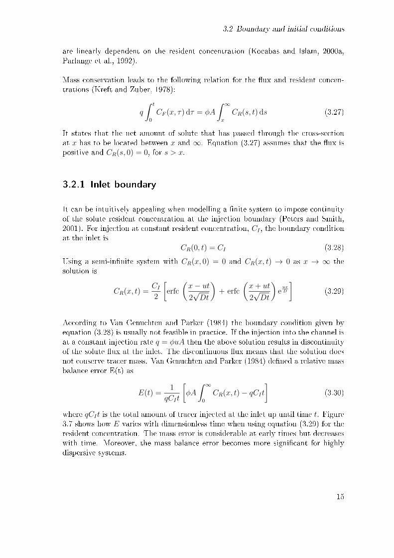
where qCIt is the total amount of tracer injected at the inlet up until time t. Figure3.7 shows how E varies with dimensionless time when using equation (3.29) for theresident concentration. The mass error is considerable at early times but decreaseswith time. Moreover, the mass balance error becomes more signi�cant for highlydispersive systems.
15

3 Tracer test theory
0 1 2 3 4 5 6 7 80
0.5
1
1.5
2
v2tD
E
Figure 3.7: Relative mass balance error, E, for the constant resident concentrationboundary condition, equation (3.28).
Continuity of the solute �ux is needed to conserve mass:[uCR −D
∂CR∂x
]x−
=
[uCR −D
∂CR∂x
]x+
(3.31)
x− stands for evaluation of the values within the bracket approaching x from theleft and x+ means evaluation approaching from the right. Simply put, solutes areneither lost nor created in a given cross-section. At the inlet boundary:[
uCR −D∂CR∂x
]x=0−
=
[uCR −D
∂CR∂x
]x=0+
(3.32)
In terms of the �ux concentration the �ux continuity gives
uCF |x=0− = uCF |x=0+ (3.33)
This gives rise to using the �ux concentration for boundary conditions. With nodispersion taking place outside the �ow-channel and insigni�cant molecular di�usionthe injection boundary condition becomes
uCI =
[uCR −D
∂CR∂x
]x=0+
(3.34)
where CI is again the injection concentration. With these assumptions the injec-tion well or fore section is modelled as a perfectly mixed region. This leads to amacroscopic discontinuity in the resident concentration (Van Genuchten and Parker,1984). This is a somewhat perplexing issue that arises due to modelling the systemon a macroscale (Peters and Smith, 2001).
16

3.2 Boundary and initial conditions
3.2.2 Outlet boundary
A similar treatment of the outlet boundary conditions leads to[uCR −D
∂CR∂x
]x=L−
=
[uCR −D
∂CR∂x
]x=L+
(3.35)
and [uCR −D
∂CR∂x
]x=L−
= uCP |x=L+ (3.36)
where CP is tracer concentration in the produced �uid. It is this outlet concentrationwhich is measured during a tracer experiment and needs to be matched with asuitable model. Handling of the exit boundary is less straight forward than at theinlet, since the output concentration is unknown. If the system, is to be modelledexplicitly as a �nite system the only option available at the outlet boundary is tomake some assumptions about the boundary. Considering this point in question canagain lead to the assumption of continuity in resident concentration. The residentconcentration is continuous at the outlet boundary if and only if
∂CR∂x
∣∣∣∣x=L−
= 0 (3.37)
Danckwerts (1953) used this boundary condition to describe �ow in packed tubularreactors. His model looks at a system with constant tracer concentration at the inlet.Regarding equation (3.36), Danckwerts argues that if ∂CR
∂x
∣∣x=L− is negative then the
outlet concentration is higher than inside the end of the packed tube. Furthermore,if the derivative is positive then the concentration would have to pass through aminimum. Danckwerts cannot intuitively see that either situation can arise whichleads him to suggest that the boundary condition has to be given by
∂CR∂x
∣∣∣∣x=L
= 0 (3.38)
to avoid these situations. Reading between the lines, it seems that his intuitiontells him that the concentration has to strictly decrease from the inlet to the outlet.This should be expected for a system with zero initial concentration and constantconcentration at the inlet. Using the same argument and assuming that the outletitself does not a�ect the outlet concentration would lead to the following boundarycondition:
∂CR∂x
∣∣∣∣x=l
= 0 (3.39)
where l ≥ L. The following extreme can just as easily be used for the same means:
∂CR∂x
∣∣∣∣x→∞
= 0 (3.40)
17

3 Tracer test theory
Brenner (1962) used the same reasoning as Danckwerts to support the adoptionof the zero gradient boundary condition at x = L. This logic cannot be used forgroundwater tracer tests where the solutes are in practice injected as �nite pulseswhich give rise to the possibility of maxima and minima of the tracer concentration.The real question is how the production boundary impacts the tracer returns. Thebest choice for l is likely somewhere between L and ∞.
Van Genuchten and Parker (1984) contended that the boundary condition givenby Danckwerts is inconsistent with the inlet condition. The zero gradient bound-ary condition at the outlet describes a process of backward mixing. Parker andVan Genuchten (1984) maintained that for �ow in porous media the only mecha-nism for back mixing is di�usion. Parker and Van Genuchten therefore reasoned thatusing equation (3.40) is likely to be the most suitable when mechanical dispersionis the dominant dispersive process.
Column experiments have been carried out to shed light on the capability of variousboundary conditions for predicting solute concentrations in porous media. Resultsof experiments support the choice of equations (3.34) and (3.40) as boundary con-ditions (Novakowski, 1992, Parker, 1984, Schwartz et al., 1999). The macroscopicdiscontinuity of tracer resident concentrations is supported by the results of columnexperiments carried out by Novakowski (1992).
The advantage of laboratory column experiments is that unlike �eld tests they canbe conducted in a controlled (as much as) environment. Lessons learnt from columnexperiments are often applied to the �eld scale, though there may be some inherentproblems with translating results from the laboratory to �eld scales. The inlets andoutlets of the �ow system are easier to control and understand in column tests thanlarge scale wells in a geothermal system. Moench (1989, 1995) proposed a model toaccount for boundary well mixing in radially convergent �eld tracer tests. His modelgives results in resident concentration but measurement of �ux concentration is mostlikely the mode of detection in �eld tests (Kocabas and Islam, 2000a, Kreft andZuber, 1978, Maloszewski and Zuber, 1997). The semi-analytical model developedby Reimus and Haga (1999), RELAP, has the option of including wellbore mixing byusing a Laplace domain transfer function. Their model assumes �ux concentrationalong the main �ow-path. Development of models describing wellbore-mixing arecertainly a theoretical improvement but it could be di�cult to evaluate the e�ectof mixing independently by di�erentiating it from results of other di�usive anddispersive processes. Selecting be�tting boundary conditions for modelling highlydispersive systems is essential for relevant model-based predictions.
18

3.3 One-dimensional analytical solutions
3.3 One-dimensional analytical solutions
The one-dimensional tracer transport equation under steady state �ow conditions isgiven by
∂C
∂t+ u
∂C
∂x= D
∂2C
∂x2(3.41)
The appropriateness of using this equation can be questionable in some cases. In thecase of a weak recirculation tracer test in a con�ned, heterogeneous aquifer the �ow�eld will probably be somewhere between linear and radial (Council, 1996, Reimusand Haga, 1999). Leibundgut et al. (2009) and Maloszewski and Zuber (1990) notethat equation (3.41) can be used for convergent radial �ow, Figure 3.8, given thatthe Peclet number Pe = D/uL > 5.
P
Figure 3.8: Convergent radial �ow around a production well, P.
The radial analogue of equation (3.41) within a uniform porous medium is
∂C
∂t+
1
r
∂(rurC)
∂r=
1
r
∂
∂r
(rDr
∂C
∂r
)(3.42)
where ur is the radial velocity, Dr the radial dispersion coe�cient and r is thedistance from the pumped well. ur has a positive value for a divergent radial �ow test(injection) but negative for a convergent test (production). A transverse dispersiveterm is generally not included in the above equation to describe convergent tests, dueto the convergence of �ow lines at the production well (Maloszewski and Zuber, 1990,Moench, 1989). Any simpli�cation of this equation will depend on assumptions maderegarding the behaviour of ur andDr (Kocabas and Islam, 2000b). The velocity term
19

3 Tracer test theory
is usually taken to be ur = B/r, where B is constant. If the dispersion is consideredconstant then
∂C
∂t+ ur
∂C
∂r= Dr
∂2C
∂r2+Dr
r
∂C
∂r(3.43)
or if Dr = αur, with α constant then
∂C
∂t+ ur
∂C
∂r= Dr
∂2C
∂r2(3.44)
For the latter type of dispersion the radial transport equation looks identical tothe linear equation, while the former has an added factor similar to the convectiveterm. The linear equation is approximately equivalent to equation (3.43) for a largeenough radial Peclet number, urr/Dr.
The radial equation is at one end of the spectrum of idealized �ow conditions inporous media. Figure 3.9 shows �ow lines for a dipole injection production doubletin an ideal uniform porous medium. The one-dimensional �ow equation is probablya better approximation to such a situation. The main reasoning for using the linearequation for geothermal systems is that apart from its simplicity it can be expectedto certain degree to match �ow channelling within geothermal reservoirs. Most ofthe �uid �ow within a geothermal reservoir is likely to be along highly permeablefractures or channels. By using a single porosity model with linear transport, thehope is to capture most of the important aspects of these �ow-channels. The pa-
Figure 3.9: Flow lines (lines with arrows) around an injection-production doublet.Diagram modi�ed from Novakowski et al. (2004).
20
3.3 One-dimensional analytical solutions
rameters used in the models should not be taken too literally but rather as somee�ective or average values for the �ow between wells.
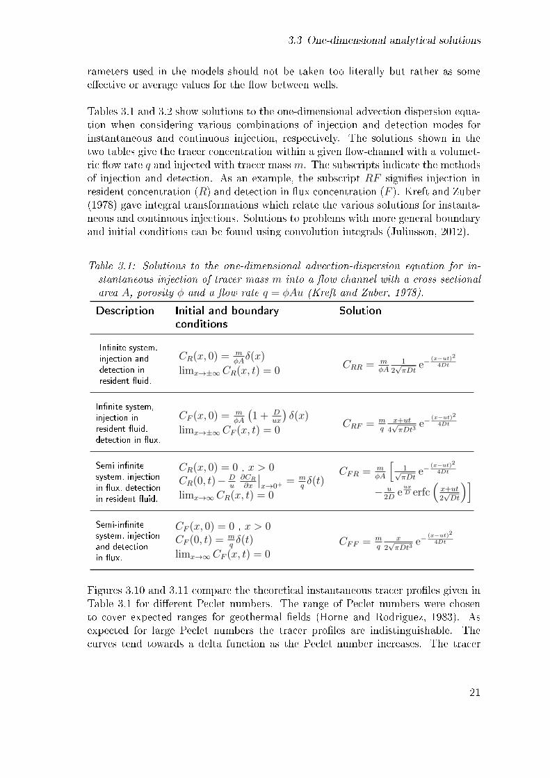
Tables 3.1 and 3.2 show solutions to the one-dimensional advection dispersion equa-tion when considering various combinations of injection and detection modes forinstantaneous and continuous injection, respectively. The solutions shown in thetwo tables give the tracer concentration within a given �ow-channel with a volumet-ric �ow rate q and injected with tracer mass m. The subscripts indicate the methodsof injection and detection. As an example, the subscript RF signi�es injection inresident concentration (R) and detection in �ux concentration (F ). Kreft and Zuber(1978) gave integral transformations which relate the various solutions for instanta-neous and continuous injections. Solutions to problems with more general boundaryand initial conditions can be found using convolution integrals (Juliusson, 2012).
Table 3.1: Solutions to the one-dimensional advection-dispersion equation for in-stantaneous injection of tracer mass m into a �ow-channel with a cross-sectionalarea A, porosity φ and a �ow rate q = φAu (Kreft and Zuber, 1978).
Description Initial and boundary Solution
conditions
In�nite system,
injection and
detection in
resident �uid.
CR(x, 0) = mφAδ(x)
limx→±∞CR(x, t) = 0CRR = m
φA1
2√πDt
e−(x−ut)2
4Dt
In�nite system,
injection in
resident �uid,
detection in �ux.
CF (x, 0) = mφA
(1 + D
ux
)δ(x)
limx→±∞CF (x, t) = 0CRF = m
qx+ut
4√πDt3
e−(x−ut)2
4Dt
Semi-in�nite
system, injection
in �ux, detection
in resident �uid.
CR(x, 0) = 0 , x > 0CR(0, t)− D
u∂CR∂x
∣∣x→0+
= mqδ(t)
limx→∞CR(x, t) = 0
CFR = mφA
[1√πDt
e−(x−ut)2
4Dt
− u2D
euxD erfc
(x+ut2√Dt
)]Semi-in�nite
system, injection
and detection
in �ux.
CF (x, 0) = 0 , x > 0CF (0, t) = m
qδ(t)
limx→∞CF (x, t) = 0CFF = m
qx
2√πDt3
e−(x−ut)2
4Dt
Figures 3.10 and 3.11 compare the theoretical instantaneous tracer pro�les given inTable 3.1 for di�erent Peclet numbers. The range of Peclet numbers were chosento cover expected ranges for geothermal �elds (Horne and Rodriguez, 1983). Asexpected for large Peclet numbers the tracer pro�les are indistinguishable. Thecurves tend towards a delta function as the Peclet number increases. The tracer
21

3 Tracer test theory
Table 3.2: Solutions to the one-dimensional advection-dispersion equation for con-tinuous injection (Kreft and Zuber, 1978).
Description Initial and boundary Solution
conditions
In�nite system,
injection and
detection in
resident �uid.
CR(x, 0) =
1 , x < 0
1
2, x = 0
0 , x > 0
limx→−∞CR(x, t) = 1limx→∞CR(x, t) = 0
CCRR = 12
erfc(x−ut2√Dt
)
In�nite system,
injection in
resident �uid,
detection in �ux.
CF (x, 0) = CR(x, 0)[1+ 2D
uδ(x)
],
where CR(x, 0) as above.limx→−∞CF (x, t) = 1limx→∞CF (x, t) = 0
CCRF = erfc(x−ut2√Dt
)+ D/u
2√πDt
e−(x−ut)2
4Dt
Semi-in�nite
system, injection
in �ux, detection
in resident �uid.
CR(x, 0) = 0 , x > 0CR(0, t)− D
u∂CR∂x
∣∣x→0+
= 1limx→∞CR(x, t) = 0
CCFR = 12
erfc(x−ut2√Dt
)+ ut√
πDte−
(x−ut)24Dt
− 12
erfc(x+ut2√Dt
)× e
uxD
[1 + u(x+ut)
D
]Semi-in�nite
system, injection
and detection
in �ux.
CF (x, 0) = 0 , x > 0CF (0, t) = 1limx→∞CF (x, t) = 0
CCFF = 12
[erfc
(x−ut2√Dt
)+ erfc
(x+ut2√Dt
)euxD
]
curves look very similar for Pe > 10. As the dispersive e�ects increase (smaller Pe)the greater the di�erence between the curves becomes. Looking at the di�erencebetween the pro�les it would seem, in theory, possible to decide which type of curvematches given tracer data if the dispersion is substantial enough. Interwell tracertests, between injection and production wells, are usually conducted by introducinga slug of tracer over a �nite period of time into the injection well. The instantaneoussolutions from Table 3.1, can be used to match the observed tracer returns at theproduction well if the tracer injection period is short enough. These solutions need tobe adjusted slightly when �tting the tracer pro�les. Focusing on the instantaneous�ux-�ux solution, the �ux concentration within the �ow-path is given by
cFF =m
q
x
2√πDt3
e−(x−ut)2
4Dt (3.45)
22
3.3 One-dimensional analytical solutions
0 1 2 30
0.5
1
1.5
tuL
CφAL
M
Pe = 1
CRR
CRF
CFR
CFF
0 1 2 30
0.5
1
1.5
tuL
CφAL
M
Pe = 2
CRR
CRF
CFR
CFF
0 1 2 30
0.5
1
1.5
tuL
CφAL
M
Pe = 10
CRR
CRF
CFR
CFF
0 1 2 30
1
2
3
tuL
CφAL
M
Pe = 100
CRR
CRF
CFR
CFF
Figure 3.10: Normalized tracer return curves for the various instantaneous one-dimensional analytical solutions and selected Peclet numbers, Pe.
Considering that the total production rate is QP at a the production well and in-voking conservation of tracer �ux (qcFF = QPCFF ) leads to
CFF (L, t) =m
QP
L
2√πDt3
e−(L−ut)2
4Dt (3.46)
for the produced �uid. The same adjustment can be made for CRF solution and thedetection in resident concentration by using conservation of tracer mass (Axelssonet al., 2005). Accounting for tracer losses to other �ow-channels gives
CFF (L, t) = ωinj
M
QP
L
2√πDt3
e−(L−ut)2
4Dt (3.47)
where M is the total injected tracer mass and ωinj is the fraction of injected �uidreaching the production well through the considered pathway. ωinj can give anindication of the expected longer term cooling e�ects deriving from injection intothe channel in question.
23

3 Tracer test theory
0 1 2 3−3
−2
−1
0
tuL
log( CφA
LM
)Pe = 1
CRR
CRF
CFR
CFF
0 1 2 3−3
−2
−1
0
tuL
log( CφA
LM
)
Pe = 2
CRR
CRF
CFR
CFF
0 1 2 3−3
−2
−1
0
tuL
log( CφA
LM
)
Pe = 10
CRR
CRF
CFR
CFF
0 1 2 3−3
−2
−1
0
tuL
log( CφA
LM
)Pe = 100
CRR
CRF
CFR
CFF
Figure 3.11: Tracer return curves for the various instantaneous one-dimensional an-alytical solutions and selected Peclet numbers, Pe. The normalized concentrationis shown on a logarithmic scale to emphasize the di�erences between the late timepredictions of the solutions.
History matching of tracer data can provide other useful information about existingconnections between wells. Rough estimates of �ow-channel volumes can be foundby �tting tracer data with theoretical pro�les (Axelsson et al., 2005) or by othermeans (Rose et al., 2004, Shook and Forsmann, 2005). Given the fraction of tracerreturns and an evaluated mean �ow-channel velocity the �ow-path pore volume is
V = φAL =qL
u= ωinj
QIL
u=m
M
QIL
u(3.48)
(Axelsson et al., 2005). Similar estimates are possible using the method of mo-ments (Rose et al., 2004, Shook and Forsmann, 2005). Assuming steady state �owconditions, the total mass recovered at the production well can be calculated using
m = QP
∫ ∞0
C(L, t) dt (3.49)
24
3.4 Matrix di�usion
The integral can be calculated by numerically integrating the tracer data. One wayis using the trapezoidal rule. The mean residence time of the �uid �owing throughthe channel is
t̄ =1
m
∫ ∞0
tC(L, t) dt (3.50)
When these integrals have been approximated then the pore volume is found by
V =m
MQI t̄ = ωinjQI t̄ (3.51)
If the reservoir is a closed system then the pore volume can easily be found byreinjecting all the produced �uid back into the reservoir. By recirculating the �uidback into the system for long enough, the injected tracer will mix evenly throughoutthe system. The pore volume is
V =M
C∞(3.52)
for a closed system, where C∞ is the constant concentration attained after in�nitetime (or long enough).
3.4 Matrix di�usion
Di�usion of solutes into stagnant water within hydrological systems can in somesituations be considerable enough that simple single-porosity �ow-channel modelsare unable to match the observed tracer breakthroughs. Models which allow fordi�usion into stagnant water may be needed (Bodin et al., 2003, Bullivant andO'Sullivan, 1985, Jensen and Horne, 1983, Maloszewski et al., 1999). For �ow alonga fracture surrounded by a low-permeability rock matrix, the tracer transport canbe modelled with a double-porosity model allowing for matrix di�usion. Keeping tolinear �ow within the main channel and considering the additional process of matrixdi�usion, the governing equation within the fracture can be taken to be (Williamset al., 2013)
∂Cf∂t
+ u∂Cf∂x−D∂
2Cf∂x2
− φmφfb
Dm∂Cm∂y
∣∣∣∣y=b
= 0 , |y| ≤ b (3.53)
when the di�usion within the matrix is given by
φm∂Cm∂t
= φmDm∂2Cm∂y2
, |y| > b (3.54)
Continuity of resident concentration is imposed at the fracture wall:
Cf = Cm , at |y| = b (3.55)
25
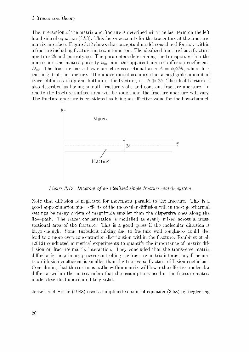
3 Tracer test theory
The interaction of the matrix and fracture is described with the last term on the lefthand side of equation (3.53). This factor accounts for the tracer �ux at the fracture-matrix interface. Figure 3.12 shows the conceptual model considered for �ow withina fracture including fracture-matrix interaction. The idealized fracture has a fractureaperture 2b and porosity φf . The parameters determining the transport within thematrix are the matrix porosity φm, and the apparent matrix di�usion coe�cient,Dm. The fracture has a �ow-channel cross-sectional area A = φf2bh, where h isthe height of the fracture. The above model assumes that a negligible amount oftracer di�uses at top and bottom of the fracture, i.e. h� 2b. The ideal fracture isalso described as having smooth fracture walls and constant fracture aperture. Inreality the fracture surface area will be rough and the fracture aperture will vary.The fracture aperture is considered as being an e�ective value for the �ow-channel.
x
y
Matrix
Fracture
2b
Figure 3.12: Diagram of an idealized single fracture matrix system.
Note that di�usion is neglected for movement parallel to the fracture. This is agood approximation since e�ects of the molecular di�usion will in most geothermalsettings be many orders of magnitude smaller than the dispersive ones along the�ow-path. The tracer concentration is modelled as evenly mixed across a cross-sectional area of the fracture. This is a good guess if the molecular di�usion islarge enough. Some turbulent mixing due to fracture wall roughness could alsolead to a more even concentration distribution within the fracture. Roubinet et al.(2012) conducted numerical experiments to quantify the importance of matrix dif-fusion on fracture-matrix interaction. They concluded that the transverse matrixdi�usion is the primary process controlling the fracture matrix interaction, if the ma-trix di�usion coe�cient is smaller than the transverse fracture di�usion coe�cient.Considering that the tortuous paths within matrix will lower the e�ective moleculardi�usion within the matrix infers that the assumptions used in the fracture-matrixmodel described above are likely valid.
Jensen and Horne (1983) used a simpli�ed version of equation (3.53) by neglecting
26

3.4 Matrix di�usion
the dispersion term within the fracture. They found a solution of the adjustedequation for a �nite injection pulse of duration ∆t. The derivation of their solutionis shown in Jensen (1983). Jensen noted that the solution of the adjusted equationfor continuous injection at constant concentration,
Cf = C0 , at |x| = 0 (3.56)
for zero initial concentration and �nite tracer concentrations as x→∞ and y →∞is (Carslaw and Jaeger, 1959)
f(x, t) = Cf (x, t)/C0 = erfc
[φmDmx
2ubφf√Dm(t− x/u)
]·H(ut− x) (3.57)
where H is the Heaviside function. The solution for a tracer slug of mass m, injectedfor a short period ∆t, can be given by
Cf (x, t) =m
q∆t[f(x, t)− f(x, t−∆t)] (3.58)
A solution for instantaneous injection can be found by taking the limit
Cf (x, t) = lim∆t→∞
m
q∆t[f(x, t)− f(x, t−∆t)] =
m
q
∂f
∂t(3.59)
Neglecting channel dispersion and solely using matrix di�usion could likely over esti-mate the fracture-matrix interaction, resulting in an overestimate of the surface areato volume ratio, b−1. This could lead to underestimation of thermal breakthrough.
Maloszewski and Zuber (1990) solved equations (3.53−3.55) including channel dis-persion for instantaneous injection in �ux concentration and detection in �ux. Theirboundary and initial conditions were
Cf (x, 0) = 0 , Cf (0, t) =m
qδ(t) , lim
x→∞Cf (x, t) = 0 , (3.60)
Cm(x, y, 0) = 0 , Cm(x, b, t) = Cf (x, t) and limy→∞
Cf (x, y, t) = 0 . (3.61)
The solution is
Cf (L, t) =ma
2πq
√Pe t0 ·
∫ t
0
exp
[−Pe(t0 − τ)2
4τt0− a2τ 2
t− τ
]dτ√
τ(t− τ)3(3.62)
with
t0 =L
u, Pe =
uL
D=L
αand a =
φm√Dm
2b(3.63)
Maloszewski et al. (1999) used the above model, with the factors in equation (3.63)as �tting parameters, to match multiple tracer pro�les. Their model also includes
27

3 Tracer test theory
additional factors describing tracer interaction with the rock matrix. Multiple tracerwith di�erent attributes can be used to support (Maloszewski et al., 1999) or in-validate (Becker and Shapiro, 2000, 2003) the idea of matrix di�usion being animportant transport process within an individual hydrological system. The �ttingparameter a can be written in terms of a formation dependent and tracer dependentpart (D∗mol):
a =φm√Dm
2b=φm√Ff
2b·√D∗mol (3.64)
Using multiple tracers with known free molecular di�usion coe�cients and estimat-ing a reasonable range for φm
√Ff it might be possible to obtain a likely range
for the surface area to volume ratio b−1. Such a procedure could help to calibratemodels for temperature predictions.
3.4.1 Tracer sorption and decay
Ideally one of the tracers used for a tracer test should be conservative and nei-ther decay nor interact with the surrounding rock formation. Finding a tracer withsuitable properties for a geothermal �eld can understandably be a di�cult task con-sidering the high temperatures, pressures and complex chemical processes takingplace within such a system. Chemicals which are relatively stable at room tem-perature can decay due to thermal degradation at conditions found in geothermalreservoirs. The thermal degradation can, at least in some cases, be described in ananalogous manner to radioactive decay
∂C
∂t= −λC (3.65)
where λ is the �rst order thermal decay rate constant (Rose et al., 2000). Reactionssuch as decay have traditionally been considered undesirable traits for tracers butsome reactive attributes may o�er a way to broaden our understanding of geothermalsystems.
Chemicals can be physically held by, adsorbed onto, and released from, or desorbedfrom, surfaces. The physical processes controlling the sorption processes will dependon the materials involved. The forces acting on a sorbing solute can be van de Waalsforces, chemical forces and ionic forces. Equations (3.53) and (3.54) can be adaptedto include tracer decay and sorption:
∂Cf∂t
+ u∂Cf∂x−D∂
2Cf∂x2
− φmφfb
Dm∂Cm∂y
∣∣∣∣y=b
= −Φs
φf− λCf (3.66)
φm∂Cm∂t
= φmDm∂2Cm∂y2
− Φs
φm− λCm (3.67)
28
3.4 Matrix di�usion
Here, Φs is the tracer transfer rate onto or into the solid phase of the formationand λf is the decay of the tracer within the �uid. The mass balance equation forthe solid phase is (Pruess et al., 2005, Reimus and Haga, 1999, Van Genuchten andWagenet, 1989)
(1− φ)ρR∂S
∂t= Φs − (1− φ)ρRλsS (3.68)
Here ρR is the density of the rock and S is the tracer surface concentration on thesolid rock phase. The decay rate of the tracer when it is sorbed, λs, is included in theabove formulation. This factor is often overlooked in the literature. It is possible toassume that the two decay rates λf and λs are equal for radioactive decay. However,the two rates will likely di�er in value for chemical degradation (Van Genuchten,1985). The reaction rate is described using sorption isotherms. Suitable isothermsare found by carrying out laboratory experiments on rock samples from a givensite or at least materials similar to those found in the �eld. The linear equilibriumadsorption isotherm
S = kC (3.69)
is widely used to describe sorption processes in hydrological settings, where k is amass based sorption partition coe�cient. The linear isotherm is a subset of the classof Freundlich isotherms given by
S = kCn (3.70)
Semi-analytical solutions are attainable for simple linear rate-limited or equilibriumisotherms (Reimus and Haga, 1999). For more complex isotherms numerical meth-ods are needed to describe the tracer transport. Sullivan et al. (2003) conductedcolumn experiments with cation-exchange tracers. They found that a linear sorp-tion model was unable to describe lithium responses at high injection concentrations.They were able to get reasonable �ts to their column data using a numerical codewhich describes multicomponent tracer transport. Cation-exchange tracers have thedisadvantage of a high detection limit and are therefore not as suitable as other trac-ers for interwell tests. However, they may be useful for single-well tests, for whichtracer losses are less of a problem (Williams et al., 2013).
The instantaneous linear equilibrium isotherm is most suitable for a rapidly sorbingtracer and in cases where the tracer concentration is fairly low. But assuming thatit is applicable we get
Rf∂Cf∂t
+ u∂Cf∂x−D∂
2Cf∂x2
− φmφfb
Dm∂Cm∂y
∣∣∣∣y=b
= −(λf +
(1− φf )ρkφf
λs
)Cf (3.71)
and
Rm∂Cm∂t
= φmDm∂2Cm∂y2
−(λf +
(1− φm)ρk
φmλs
)Cm (3.72)
where
Rf = 1 +(1− φf )ρk
φfand Rm = 1 +
(1− φm)ρk
φm
29

3 Tracer test theory
Rf and Rm will be referred to as the fracture and matrix retardation factors, re-spectively. The fracture retardation factor, Rf , is sometimes given in terms of asurface-area-based partition coe�cient Ka (Williams et al., 2013):
Rf = 1 +Ka
b
Now the e�ective fracture half aperture, b, can be found by evaluating the fractureretardation factor by matching tracer test pro�les using sorbing tracers, assumingthat the surface-area-based sorption partition coe�cient, Ka, is known.
30

4 Thermal breakthrough
Thermal breakthrough predictions are based on the similarity of the transport equa-tions describing the advancement of tracers and thermal fronts. The general tracertransport equation for steady �ow conditions is
Rtracer
∂C
∂t+ u · ∇C = D∇2C (4.1)
while the thermal changes can be described using (Bodvarsson, 1972)
Rthermal
∂T
∂t+ u · ∇T = κ∇2T (4.2)
where
Rtracer = 1 +(1− φ)ρk
φand Rthermal = 1 +
(1− φ)ρRcRφρwcw
(4.3)
are the tracer and thermal retardation coe�cients, respectively. Here
κ =kth
φρwcw(4.4)
is the thermal di�usivity and kth is the thermal conductivity of the formation. Notethat k is again the mass based sorption coe�cient, ρ is density and c is the spe-ci�c heat capacity. The subscripts R and w denote values for the rock and �uid,respectively. It is assumed in the derivation of equation (4.3) that the temperaturesof the �uid and porous rock are instantaneously equilibrated. The two transportequations shown above take the same relative form with similar factors. Notice thatthe two transport equations contain the same sort of convective term. If there areno di�usive or dispersive e�ects then the ratio of the arrival time of the thermalfront to the tracer front is Rthermal/Rtracer. The thermal di�usivity is analogous tothe tracer di�usion/dispersion term.
If we keep to the conceptual model shown in Figure 3.12 describing transport alonga �ssure then the thermal transport can be described by
Rthermal,f
∂Tf∂t
+ u∂Tf∂x−D∂
2Tf∂x2
− κ′mb
∂Tm∂y
∣∣∣∣y=b
= 0 , |y| ≤ b (4.5)
and∂Tm∂t
= κm∂2Tm∂x2
, |y| > b (4.6)
31
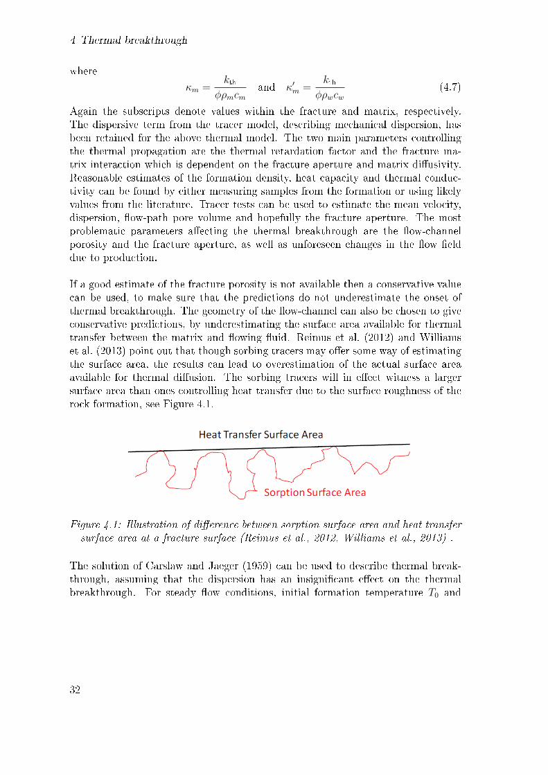
4 Thermal breakthrough
where
κm =kth
φρmcmand κ′m =
kthφρwcw
(4.7)
Again the subscripts denote values within the fracture and matrix, respectively.The dispersive term from the tracer model, describing mechanical dispersion, hasbeen retained for the above thermal model. The two main parameters controllingthe thermal propagation are the thermal retardation factor and the fracture ma-trix interaction which is dependent on the fracture aperture and matrix di�usivity.Reasonable estimates of the formation density, heat capacity and thermal conduc-tivity can be found by either measuring samples from the formation or using likelyvalues from the literature. Tracer tests can be used to estimate the mean velocity,dispersion, �ow-path pore volume and hopefully the fracture aperture. The mostproblematic parameters a�ecting the thermal breakthrough are the �ow-channelporosity and the fracture aperture, as well as unforeseen changes in the �ow �elddue to production.
If a good estimate of the fracture porosity is not available then a conservative valuecan be used, to make sure that the predictions do not underestimate the onset ofthermal breakthrough. The geometry of the �ow-channel can also be chosen to giveconservative predictions, by underestimating the surface area available for thermaltransfer between the matrix and �owing �uid. Reimus et al. (2012) and Williamset al. (2013) point out that though sorbing tracers may o�er some way of estimatingthe surface area, the results can lead to overestimation of the actual surface areaavailable for thermal di�usion. The sorbing tracers will in e�ect witness a largersurface area than ones controlling heat transfer due to the surface roughness of therock formation, see Figure 4.1.
Figure 4.1: Illustration of di�erence between sorption surface area and heat transfersurface area at a fracture surface (Reimus et al., 2012, Williams et al., 2013) .
The solution of Carslaw and Jaeger (1959) can be used to describe thermal break-through, assuming that the dispersion has an insigni�cant e�ect on the thermalbreakthrough. For steady �ow conditions, initial formation temperature T0 and
32
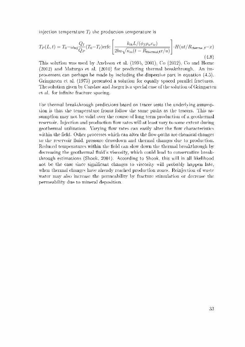
injection temperature TI the production temperature is
TP (L, t) = T0−ωinj
QI
QP
(T0−TI)erfc
[kthL/(φfρwcw)
2bu√κm(t−Rthermal,fx/u)
]·H(ut/Rthermal,f−x)
(4.8)This solution was used by Axelsson et al. (1995, 2001), Co (2012), Co and Horne(2012) and Maturgo et al. (2010) for predicting thermal breakthrough. An im-provement can perhaps be made by including the dispersive part in equation (4.5).Gringarten et al. (1975) presented a solution for equally spaced parallel fractures.The solution given by Carslaw and Jaeger is a special case of the solution of Gringartenet al. for in�nite fracture spacing.
For thermal breakthrough predictions based on tracer tests the underlying assump-tion is that the temperature fronts follow the same paths as the tracers. This as-sumption may not be valid over the course of long term production of a geothermalreservoir. Injection and production �ow rates will at least vary to some extent duringgeothermal utilization. Varying �ow rates can easily alter the �ow characteristicswithin the �eld. Other processes which can alter the �ow-paths are chemical changesto the reservoir �uid, pressure drawdown and thermal changes due to production.Reduced temperatures within the �eld can slow down the thermal breakthrough bydecreasing the geothermal �uid's viscosity, which could lead to conservative break-through estimations (Shook, 2001). According to Shook, this will in all likelihoodnot be the case since signi�cant changes to viscosity will probably happen late,when thermal changes have already reached production zones. Reinjection of wastewater may also increase the permeability by fracture stimulation or decrease thepermeability due to mineral deposition.
33


5 Numerical modelling
Recent theoretical work and column experiments show that new types of tracersmay be a promising prospect for characterizing interwell connectivity in geothermalsystems. Tracers that are sensitive to fracture matrix interfaces can in theory beused to advance cooling predictions.
Analytical solutions of tracer transport are limited to solving mass transport equa-tions which include processes which are simple to formulate. Slightly more compli-cated models can be solved using semi-analytical Laplace methods. An advantage ofusing Laplacian solutions is that convolution integrals become simple multiplicationsin Laplace space (Reimus and Haga, 1999). However, for more involved problemswith highly nonlinear factors, neither analytical nor semi-analytical methods are anoption. In those situations the researcher needs to turn to numerical simulationmethods.
Numerical methods may seem unappealing to some. Reasons may be that numericalsimulations may take a long time to give results and can give erroneous results.Ever increasing computer speeds and improved numerical simulation methods makethose drawbacks a lesser issue. Semi-numerical methods can also have problemswith numerical errors. Furthermore, semi-analytical methods can in some casesbecome cumbersome, if not impractical, and may have longer run-times than thecorresponding numerical method (Juliusson and Horne, 2012, Jung and Pruess, 2012,Maier and Kocabas, 2013a).
A numerical �nite volume method is described in the following sections. The numer-ical code used is based on a method laid out in Patankar (1980). The method used afully implicit scheme with upstream weighting and rectangular �nite volumes. Thisscheme is chosen for its simplicity, ease of implementing boundary conditions androbustness. It proves to give fairly good accuracy for encountered problems. Othermethods, which can improve numerical accuracy, may also be considered (Croucherand O'Sullivan, 1998, Croucher et al., 2004).
35

5 Numerical modelling
5.1 One-dimensional �ow-paths
The one-dimensional advection-dispersion equation including source terms, S∗, isgiven by
∂C
∂t+ u
∂C
∂x= D
∂2C
∂x2+ S∗ (5.1)
W P E
w e
δxw δxe
∆x
Figure 5.1: Typical grid-point cluster for the one-dimensional problem.
The one-dimensional �nite volume solution to the advection dispersion equation isfound by integrating the transport equation over the �nite volume, of length ∆x,shown in Figure 5.1:∫ w
e
∂C
∂tdx =
∫ w
e
(D∂2C
∂x2− u∂C
∂x+ S∗
)dx (5.2)
Solving the integrals we �nd that
∆x∂CP∂t
= D
(∂C
∂x
∣∣∣∣e
− ∂C
∂x
∣∣∣∣w
)− u(Ce − Cw) + ∆xS̄∗ (5.3)
The concentration of the nodal point P was assumed to be a good enough averageconcentration over the whole volume for the evaluation of the time derivative. S̄∗ isthe average value of the source term over the control volume. Some decision needsto be made on how to approximate the terms on the control volume's boundary.The derivatives can be approximated using �nite di�erences:
∂C
∂x
∣∣∣∣e
≈ CE − CPδxe
and∂C
∂x
∣∣∣∣w
≈ CP − CWδxw
(5.4)
The W and E denote values given at the closest upstream and downstream neigh-bouring nodes. For an upwind scheme with positive �ow, u > 0, being from left toright in Figure 5.1 we have
Cw ≈ CW and Ce ≈ CP (5.5)
The time derivative is given implicitly by
∆x∂C
∂t≈ ∆x
∆t(CP − C0
P ) (5.6)
36

5.1 One-dimensional �ow-paths
where ∆t is the current time step and C0P is the element's concentration from the
previous time step. Substituting equations (5.4−5.6) into equation (5.3) gives
aPCP = aWCW + aECE + d (5.7)
with
aW =D
δxw
aE =D
δxe+ u
a0P =
∆x
∆td = a0
PC0P + S̄∗
aP = aW + aE + a0P
(5.8)
These parameters can be made more general for positve and negative velocities, u:
aW =D
δxw+ max(−u, 0)
aE =D
δxe+ max(u, 0)
a0P =
∆x
∆td = a0
PC0P + S̄∗
aP = aW + aE + a0P
(5.9)
In matrix form equation (5.7) is expressed as
BC = d (5.10)
where B is an N×N tridiagonal matrix, C =[C1 C2 ... CN
]T, N is the number
of elements in the grid and d =[d1 d2 ... dN
]T, see �gure 5.2. Equation (5.10)
can be solved using various known matrix solvers. The optimum method for solvingthe matrix equation will depend on the location of the non-zero elements of matrixB. The Thomas Algorithm is a well known algorithm for solving tridiagonal systemsof equations. All of the code written for this thesis was implemented using MATLAB.MATLAB has an inbuilt matrix solver which can be called upon using the backslashoperator.
37

5 Numerical modelling
Figure 5.2: One-dimensional �nite volume grid with N elements.
5.2 Fracture including matrix di�usion
The equations describing the transport within a �ssure with matrix di�usion canbe solved in the same way as outlined for the one-dimensional transport equation.For the two-dimensional case the �nite volumes are as depicted in Figure 5.3. Asbefore the positive x direction is from W to E, while the positive y direction is frompoint S to point N . With the additional spatial dimension, the discredized equationbecomes
aPCP = aWCW + aECE + aSCS + aNCN + d (5.11)
W P E
N
S
w
e
n
s
∆x
∆y x
y
Figure 5.3: Control volume for the two-dimensional situation.
For transport within the matrix with matrix di�usion coe�cients Dmx and Dmy
along the y and x axis, respectively, see Figure 3.12:
∂Cm∂t
= Dmy∂2Cm∂y2
+Dmx∂2Cm∂x2
(5.12)
38
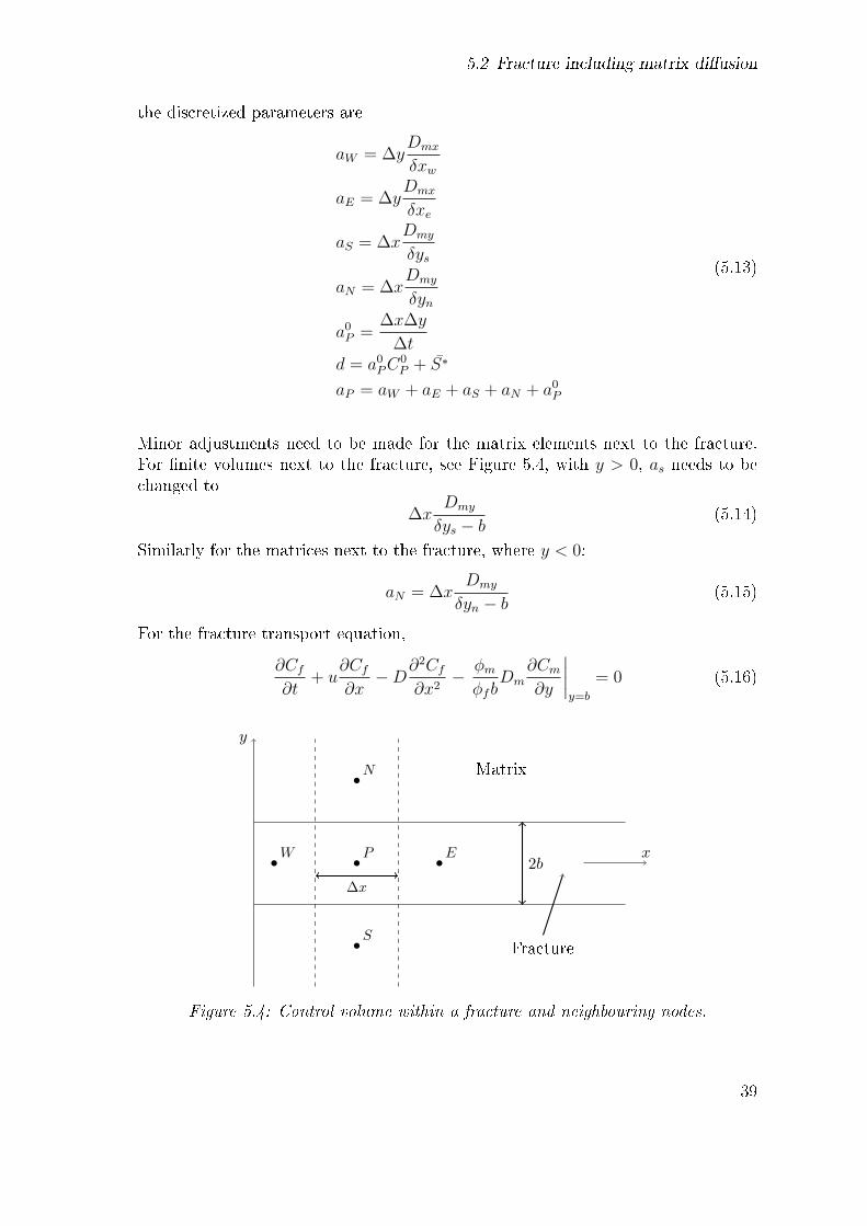
5.2 Fracture including matrix di�usion
the discretized parameters are
aW = ∆yDmx
δxw
aE = ∆yDmx
δxe
aS = ∆xDmy
δys
aN = ∆xDmy
δyn
a0P =
∆x∆y
∆td = a0
PC0P + S̄∗
aP = aW + aE + aS + aN + a0P
(5.13)
Minor adjustments need to be made for the matrix elements next to the fracture.For �nite volumes next to the fracture, see Figure 5.4, with y > 0, as needs to bechanged to
∆xDmy
δys − b(5.14)
Similarly for the matrices next to the fracture, where y < 0:
aN = ∆xDmy
δyn − b(5.15)
For the fracture transport equation,
∂Cf∂t
+ u∂Cf∂x−D∂
2Cf∂x2
− φmφfb
Dm∂Cm∂y
∣∣∣∣y=b
= 0 (5.16)
x
y
Matrix
Fracture
2bP
N
S
W E
∆x
Figure 5.4: Control volume within a fracture and neighbouring nodes.
39
5 Numerical modelling
the numerical parameters are
aW = 2bD
δxw+ max(−u, 0)
aE = 2bD
δxe+ max(u, 0)
aS =φm∆x
φf
Dmy
δys − b
aN =φm∆x
φf
Dmy
δyn − b
a0P =
2∆xb
∆td = a0
PC0P + S̄∗
aP = aW + aE + aS + aN + a0P
(5.17)
Due to the symmetry of the fracture-matrix model, the number of equations canbe reduced. The tracer concentration need only be evaluated within the matrix fory > 0. Using this method then
aP = aW + aE + 2aN + a0P (5.18)
within the fracture. To avoid possible numerical imprecision the values of aN withinthe fracture and aS inside the matrix next to the fracture were computed using
δys − b = δyn − b = ymatrix element (5.19)
where ymatrix element is the distance of the matrix element's node from the fracture.
The thermal transport equations can be formulated in the same way. The parametersfor the tracer case need only be adjusted using simple algebraic methods.
5.3 Implementing initial and boundary conditions
Injection and detection in �ux concentration can be easily accounted for by notingthat the tracer �ux per unit area at an injection boundary is
Φw = uCw −D∂C
∂x
∣∣∣∣w
= uCI (5.20)
and the outward �ux per unit area is
Φe = uCe −D∂C
∂x
∣∣∣∣e
(5.21)
40
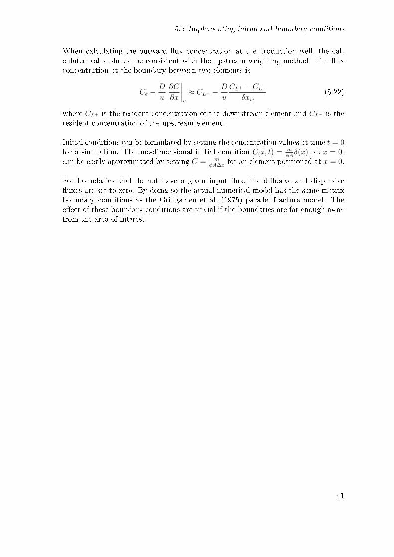
5.3 Implementing initial and boundary conditions
When calculating the outward �ux concentration at the production well, the cal-culated value should be consistent with the upstream weighting method. The �uxconcentration at the boundary between two elements is
Ce −D
u
∂C
∂x
∣∣∣∣e
≈ CL+ − D
u
CL+ − CL−
δxw(5.22)
where CL+ is the resident concentration of the downstream element and CL− is theresident concentration of the upstream element.
Initial conditions can be formulated by setting the concentration values at time t = 0for a simulation. The one-dimensional initial condition C(x, t) = m
φAδ(x), at x = 0,
can be easily approximated by setting C = mφA∆x
for an element positioned at x = 0.
For boundaries that do not have a given input �ux, the di�usive and dispersive�uxes are set to zero. By doing so the actual numerical model has the same matrixboundary conditions as the Gringarten et al. (1975) parallel fracture model. Thee�ect of these boundary conditions are trivial if the boundaries are far enough awayfrom the area of interest.
41

6 Matching tracer data
Parameter estimation is typically carried out by �nding the model parameters whichminimize the di�erence between model predictions and measured data in some sense.For the estimation of tracer transport parameters in this work the chosen objectivefunction is the sum of the square di�erences between the tracer data and modelforecasts. The objective function used here is
f(z) =1
2‖(rj(z)‖2 =
1
2r(z)T r(z) =
1
2
n∑j=1
(rj(z))2 (6.1)
where r is a column vector of length n containing the residual di�erence betweenthe model predictions and observed data. The T denotes a vector transpose and zis a vector of the unknown model parameters. Given measured data,
Cd = [Cd1 Cd
2 . . . Cdi . . . Cd
n−1 Cdn]T (6.2)
and model predictions,
Cm = [Cm1 Cm
2 . . . Cmi . . . Cm
n−1 Cmn ]T (6.3)
then the residual vector isr(z) = Cm −Cd (6.4)
Using equation (6.1) gives equal weights to each data point in the �tting process. Theobjective function may be altered to accommodate for the possibility of assigningweights to each data point:
f(z) =1
2
n∑j=1
wj(rj(z))2 (6.5)
where wj are positive weights, which can be increased or decreased depending onthe reliability of a measured value.
Multiple methods can be found in the literature for minimizing non-linear functionssuch as the ones given in equations (6.1) and (6.5). Variants of the Levenberg-Marquardt algorithm were found to work quite well for problems presented in thisthesis. The Levenberg-Marquardt has proven to be suitable for many geothermalapplications (Finsterle, 2007). However, more robust, global minimizers may bedesirable for complex simulation problems (Plasencia et al., 2012).
43

6 Matching tracer data
6.1 The Levenberg-Marquardt algorithm
The Levenberg-Marquardt algorithm is a damped Gauss-Newton minimization meth-od. The Gauss-Newton method is based on a local Taylor approximation of theresiduals
r(z + h) ≈ r(z) + J(z)h (6.6)
where J is the Jacobian matrix with elements Jij = ∂ri/∂zj. For each iteration ofthe Gauss-Newton method the step taken h is found by solving(
JTJ)h = −JTr (6.7)
The Gauss-Newton method may converge rapidly towards a minimum if the initialguess z0 for the parameter vector z is close enough to the minimizer. However, thematrix JTJ can be ill-conditioned, resulting in unacceptable global behaviour forthe Gauss-Newton method.
Levenberg (1944) and thereafter Marquardt (1963) advocated using a damped ver-sion of the Gauss-Newton algorithm. The minimization steps for the Levenberg-Marquardt algorithm are found by solving(
JTJ + µD)h = −JTr (6.8)
where D is a positive de�nite, diagonal matrix and µ is an adjustable dampeningparameter. The dampening parameter is chosen to be positive to keep the totaldampening matrix µD positive de�nite. For small values of µ the above dampedmethod gives approximately Gauss-Newton steps h. For large values of the damp-ening factor, the Levenberg-Marquardt method takes small steps in the direction ofsteepest descent.
Madsen and Nielsen (2010) give a pseudocode for the Levenberg-Marquardt algo-rithm, see Algorithm 1. They recommend using an initial dampening factor givenby
µ0 = τ ·max [Aii] , where A = J(z0)TJ(z0) (6.9)
τ is given by the user. According to Madsen and Nielsen it should be chosen to besmall (∼ 10−6) for initial guesses close to the minimum but larger for bad guesses.This relates to wanting the steps to be close to the Gauss-Newton steps within thecone of in�uence but choosing steps closer to ones given by steepest descent meth-ods for parameters far away from the minimum. The dampening parameter, µ, isadjusted within Algorithm 1 depending on how well the procedure is progressing.The parameters kmax, ε1 and ε2 are chosen to give reasonable limits to the maxi-mum number of iterations, minimum length of the gradient and smallest step size,respectively. If any of these limits are broken then the code stops. Breaking of thelatter two limits may indicate that the method has converged upon a minimum.
44
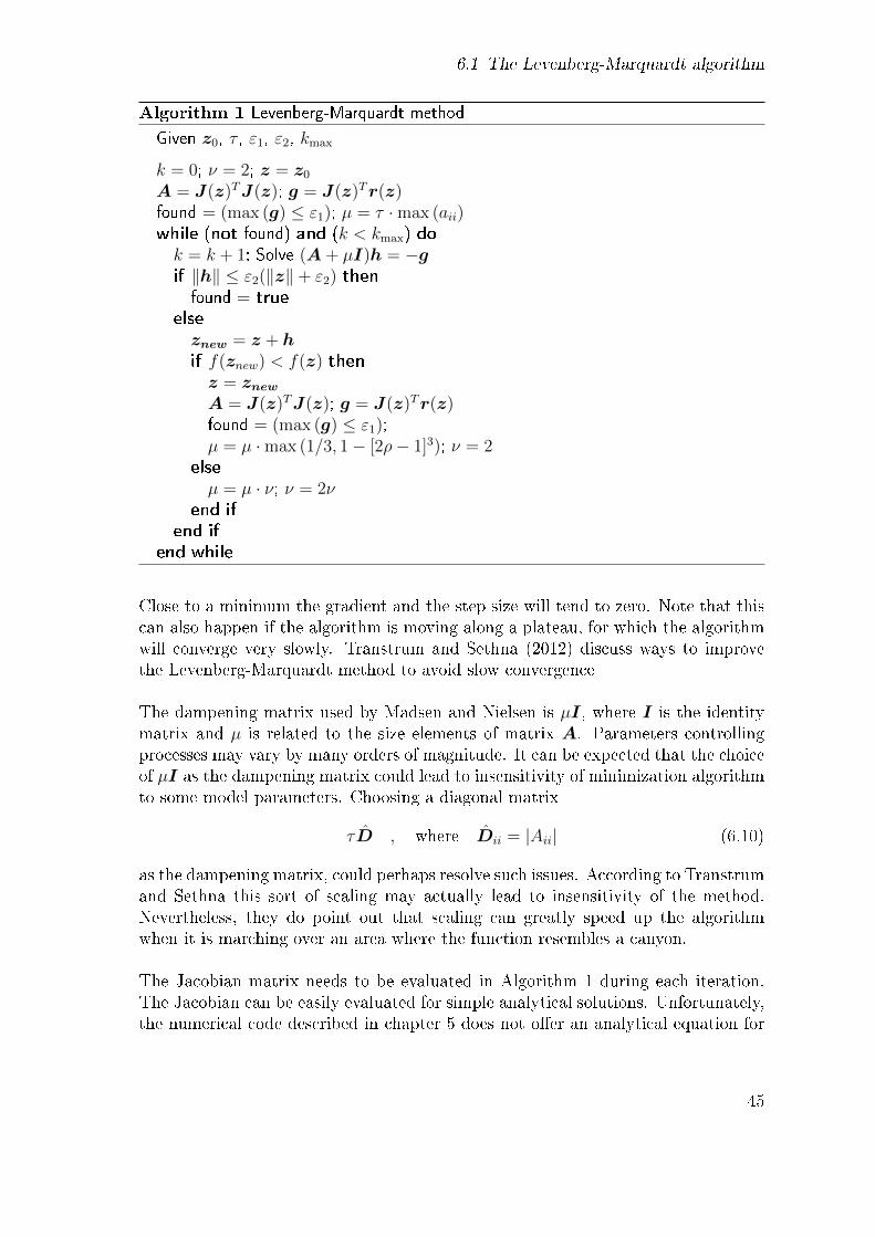
6.1 The Levenberg-Marquardt algorithm
Algorithm 1 Levenberg-Marquardt method
Given z0, τ , ε1, ε2, kmax
k = 0; ν = 2; z = z0
A = J(z)TJ(z); g = J(z)Tr(z)found = (max (g) ≤ ε1); µ = τ ·max (aii)while (not found) and (k < kmax) dok = k + 1; Solve (A + µI)h = −gif ‖h‖ ≤ ε2(‖z‖+ ε2) then
found = true
else
znew = z + hif f(znew) < f(z) thenz = znew
A = J(z)TJ(z); g = J(z)Tr(z)found = (max (g) ≤ ε1);µ = µ ·max (1/3, 1− [2ρ− 1]3); ν = 2
else
µ = µ · ν; ν = 2νend if
end if
end while
Close to a minimum the gradient and the step size will tend to zero. Note that thiscan also happen if the algorithm is moving along a plateau, for which the algorithmwill converge very slowly. Transtrum and Sethna (2012) discuss ways to improvethe Levenberg-Marquardt method to avoid slow convergence
The dampening matrix used by Madsen and Nielsen is µI, where I is the identitymatrix and µ is related to the size elements of matrix A. Parameters controllingprocesses may vary by many orders of magnitude. It can be expected that the choiceof µI as the dampening matrix could lead to insensitivity of minimization algorithmto some model parameters. Choosing a diagonal matrix
τD̂ , where D̂ii = |Aii| (6.10)
as the dampening matrix, could perhaps resolve such issues. According to Transtrumand Sethna this sort of scaling may actually lead to insensitivity of the method.Nevertheless, they do point out that scaling can greatly speed up the algorithmwhen it is marching over an area where the function resembles a canyon.
The Jacobian matrix needs to be evaluated in Algorithm 1 during each iteration.The Jacobian can be easily evaluated for simple analytical solutions. Unfortunately,the numerical code described in chapter 5 does not o�er an analytical equation for
45
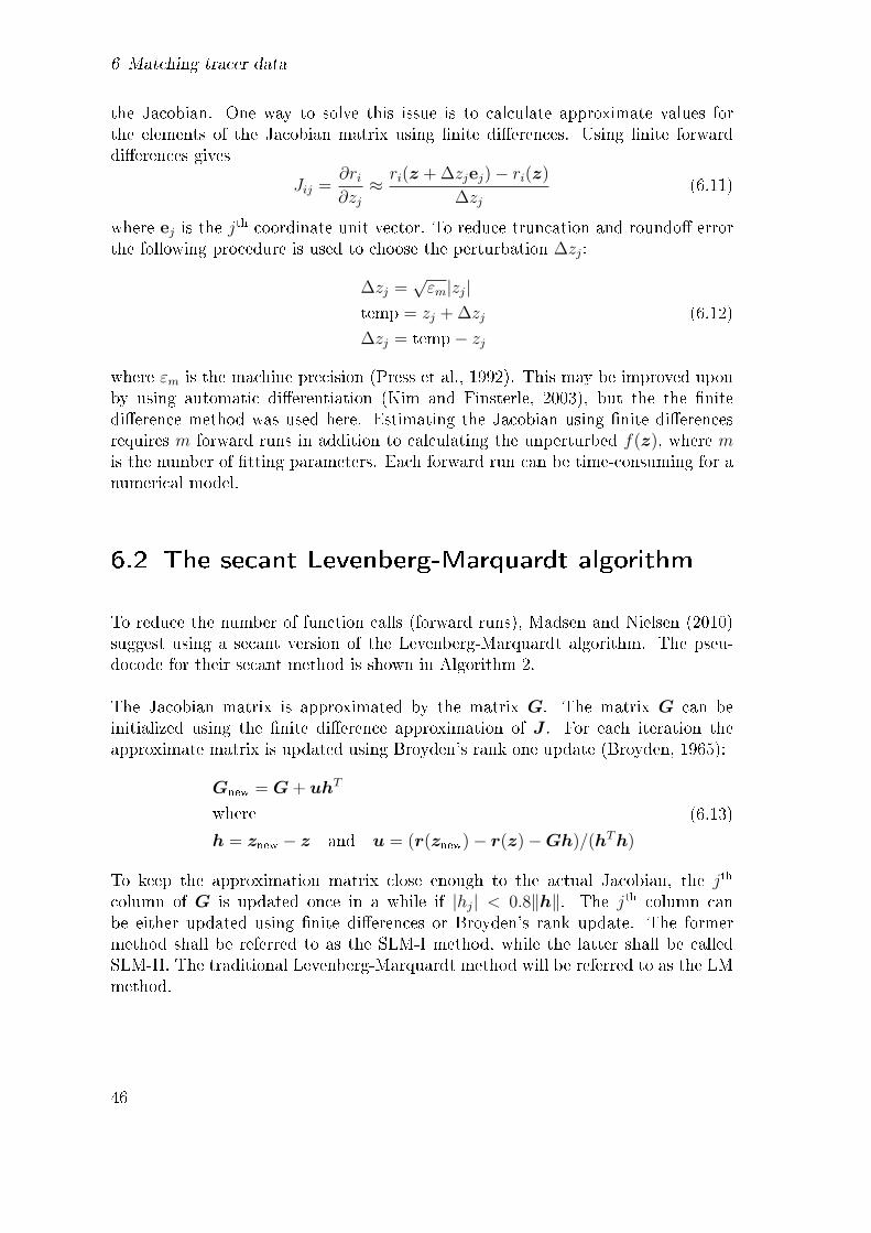
6 Matching tracer data
the Jacobian. One way to solve this issue is to calculate approximate values forthe elements of the Jacobian matrix using �nite di�erences. Using �nite forwarddi�erences gives
Jij =∂ri∂zj≈ ri(z + ∆zjej)− ri(z)
∆zj(6.11)
where ej is the jth coordinate unit vector. To reduce truncation and roundo� errorthe following procedure is used to choose the perturbation ∆zj:
∆zj =√εm|zj|
temp = zj + ∆zj
∆zj = temp− zj(6.12)
where εm is the machine precision (Press et al., 1992). This may be improved uponby using automatic di�erentiation (Kim and Finsterle, 2003), but the the �nitedi�erence method was used here. Estimating the Jacobian using �nite di�erencesrequires m forward runs in addition to calculating the unperturbed f(z), where mis the number of �tting parameters. Each forward run can be time-consuming for anumerical model.
6.2 The secant Levenberg-Marquardt algorithm
To reduce the number of function calls (forward runs), Madsen and Nielsen (2010)suggest using a secant version of the Levenberg-Marquardt algorithm. The pseu-docode for their secant method is shown in Algorithm 2.
The Jacobian matrix is approximated by the matrix G. The matrix G can beinitialized using the �nite di�erence approximation of J . For each iteration theapproximate matrix is updated using Broyden's rank one update (Broyden, 1965):
Gnew = G + uhT
where
h = znew − z and u = (r(znew)− r(z)−Gh)/(hTh)
(6.13)
To keep the approximation matrix close enough to the actual Jacobian, the jth
column of G is updated once in a while if |hj| < 0.8‖h‖. The jth column canbe either updated using �nite di�erences or Broyden's rank update. The formermethod shall be referred to as the SLM-I method, while the latter shall be calledSLM-II. The traditional Levenberg-Marquardt method will be referred to as the LMmethod.
46

6.2 The secant Levenberg-Marquardt algorithm
Algorithm 2 Secant version of the Levenberg-Marquardt method
Given z0, τ , ε1, ε2, kmax
k = 0; z = z0; G = J(z); ν = 2; j = 0A = GTG; g = GTr(z)found = (max (g) ≤ ε1); µ = τ ·max (aii)while (not found) and (k < kmax) dok = k + 1; Solve (A + µI)h = −gif ‖h‖ ≤ ε2(‖z‖+ ε2) then
found = true
else
j = mod (j,n) + 1if |hj| < 0.8‖h‖ then
Update G by a �nite di�erence approximationend if
znew = z + hUpdate G using Broyden's rank one updateUpdate µ as in Algorithm 1if f(znew) < f(z) thenz = znew
end if
g = GTr(z); found = (max (g) ≤ ε1);end if
end while
47
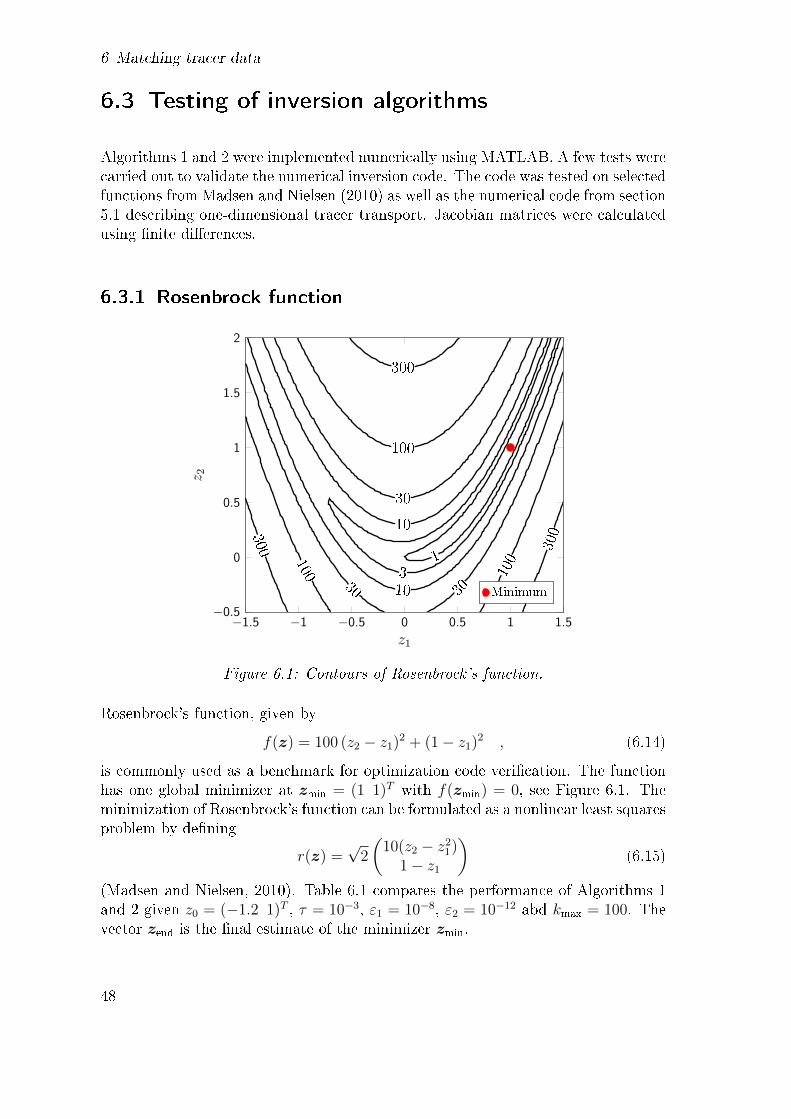
6 Matching tracer data
6.3 Testing of inversion algorithms
Algorithms 1 and 2 were implemented numerically using MATLAB. A few tests werecarried out to validate the numerical inversion code. The code was tested on selectedfunctions from Madsen and Nielsen (2010) as well as the numerical code from section5.1 describing one-dimensional tracer transport. Jacobian matrices were calculatedusing �nite di�erences.
6.3.1 Rosenbrock function
−1.5 −1 −0.5 0 0.5 1 1.5−0.5
0
0.5
1
1.5
2
100
300
30
300
100
300
100
30 3010
1
10
3
z1
z 2
Minimum
Figure 6.1: Contours of Rosenbrock's function.
Rosenbrock's function, given by
f(z) = 100 (z2 − z1)2 + (1− z1)2 , (6.14)
is commonly used as a benchmark for optimization code veri�cation. The functionhas one global minimizer at zmin = (1 1)T with f(zmin) = 0, see Figure 6.1. Theminimization of Rosenbrock's function can be formulated as a nonlinear least squaresproblem by de�ning
r(z) =√
2
(10(z2 − z2
1)1− z1
)(6.15)
(Madsen and Nielsen, 2010). Table 6.1 compares the performance of Algorithms 1and 2 given z0 = (−1.2 1)T , τ = 10−3, ε1 = 10−8, ε2 = 10−12 abd kmax = 100. Thevector zend is the �nal estimate of the minimizer zmin.
48

6.3 Testing of inversion algorithms
Table 6.1: Performance of optimization algorithms for solving the Rosenbrock prob-lem.
MethodDampening Function ‖∇f‖ f(zend) Iterations
matrix evaluations
LM µI 47 3.7 · 10−9 1.7 · 10−17 16
LM τD̂ 68 4.5 · 10−10 1.6 · 10−19 29
SLM-I µI 51 4.2 · 10−9 1.6 · 10−19 28
SLM-I τD̂ 32 6.8 · 10−10 4.2 · 10−22 18SLM-II µI 51 4.2 · 10−9 1.6 · 10−19 28
SLM-II τD̂ 32 6.8 · 10−10 4.2 · 10−22 18
The results were inconclusive regarding which dampening matrix is preferable. Theidentity matrix proved better for the LM method but the other dampening matrixtype worked better for the secant methods.
The results that should be focussed on are the number of function calls that themethods used, since the limiting factor for �tting numerically simulated models todata are the forward runs. In that respect, the secant methods using the identitymatrix performed similarly to the LM method. The secant methods do show somepromise, in that when using the second dampening matrix type they needed fewerfunction calls. However, the secant methods need more iterations to reach theminimum, which indicates that they are less robust than the LM method. Thedi�erences between the two secant methods were imperceptible.
6.3.2 Scaling
Madsen and Nielsen (2010) demonstrated the importance of the relative di�erencebetween the scales of �tting parameters by solving Meyer's problem. Meyer's prob-lem is given by the residual function
ri(z) = yi − z1 exp
(z2
ti + z3
), i = 1, ..., 16 (6.16)
with ti = 45 + 5i and yi takes the values shown in Table 6.2.
Meyer's problem has a minimum at zmin ≈ (5.61 · 10−3 6.18 · 103 3.45 · 102)T withf(zmin) ≈ 43.97 (Madsen and Nielsen, 2010). Table 6.3 compares the performanceof Algorithms 1 and 2 given z0 = (2 · 10−2 4 · 103 2.5 · 102)T , τ = 1, ε1 = 10−6,ε2 = 10−10 abd kmax = 500.
49

6 Matching tracer data
Table 6.2: Values used for Meyer's problem.
i yi i yi i yi
1 34780 7 11540 12 51472 28610 8 9744 13 44273 23650 9 8261 14 38204 19630 10 7030 15 33075 16370 11 6005 16 28726 13720
The secant methods performed somewhat di�erently when solving Meyer's problem.Table 6.3 gives the 2-norm of the gradient by calculating the gradient using ∇f =JTr, where J is found at the �nal point using �nite di�erences. If the gradient at the�nal iteration was approximated by GTr, then the SLM-II method underestimatedthe size of the gradient by one to two orders of magnitude. The di�erences betweenusing G and J for this problem (and Rosenbrock's) appear to be negligible for theother SLM method around the minimizer.
Table 6.3: Performance of optimization algorithms for solving the Meyer problem.
MethodDampening Function ‖∇f‖ f(zend) Iterations
matrix evaluations
LM µI 710 0.041 43.97 182
LM τD̂ 521 0.54 43.97 137
SLM-I µI 432 0.12 43.97 258
SLM-I τD̂ 420 0.25 43.97 250SLM-II µI 449 0.13 43.97 268
SLM-II τD̂ 382 0.10 43.97 227
According to Madsen and Nielsen (2010) it is possible to reduce the number ofiterations needed to reach a good approximation for the minimizer by rescaling thisproblem. Using rescaling, Madsen and Nielsen were able to halve the number ofrequired iterations, from 175 to 88, using Algorithm 1 and a Jacobian found usingan analytical equation. Madsen and Nielsen reformulated the problem using
ri(z∗) = 10−3 · yi − z∗1 exp
10z∗2ui + z∗3
, i = 1, ..., 16 (6.17)
where ui = 0.45 + 0.05i and the new parameter vector z∗ is related to z as follows
z∗ = [10−3e13z1 10−3z2 10−2z3] (6.18)
The LM method using numerical di�erentiation solved the scaled problem by usingthe same number of iterations, 88, as the analytical one, see Table 6.4. Again, fewer
50
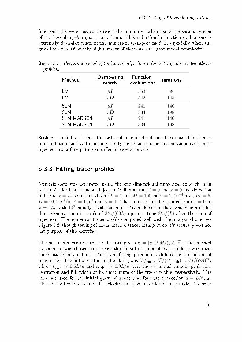
6.3 Testing of inversion algorithms
function calls were needed to reach the minimizer when using the secant versionof the Levenberg�Marquardt algorithm. This reduction in function evaluations isextremely desirable when �tting numerical transport models, especially when thegrids have a considerably high number of elements and great model complexity
Table 6.4: Performance of optimization algorithms for solving the scaled Meyerproblem.
MethodDampening Function
Iterationsmatrix evaluations
LM µI 353 88
LM τD̂ 542 145
SLM µI 241 140
SLM τD̂ 334 198SLM-MADSEN µI 241 140
SLM-MADSEN τD̂ 334 198
Scaling is of interest since the order of magnitude of variables needed for tracerinterpretation, such as the mean velocity, dispersion coe�cient and amount of tracerinjected into a �ow-path, can di�er by several orders.
6.3.3 Fitting tracer pro�les
Numeric data was generated using the one dimensional numerical code given insection 5.1 for instantaneous injection in �ux at time t = 0 and x = 0 and detectionin �ux at x = L. Values used were L = 1 km,M = 100 kg, u = 2 ·10−4 m/s, Pe = 5,D = 0.04 m2/s, A = 1 m2 and φ = 1. The numerical grid extended from x = 0 tox = 5L, with 103 equally sized elements. Tracer detection data was generated fordimensionless time intervals of 3tu/(60L) up until time 3tu/(L) after the time ofinjection. The numerical tracer pro�le compared well with the analytical one, seeFigure 6.2, though testing of the numerical tracer transport code's accuracy was notthe purpose of this exercise.
The parameter vector used for the �tting was z = [u D M/(φA)]T . The injectedtracer mass was chosen to increase the spread in order of magnitude between thethree �tting parameters. The given �tting parameters di�ered by six orders ofmagnitude. The initial vector for the �tting was [L/tpeak L
2/(4twidth) 1.5M/(φA)]T ,where tpeak ≈ 0.6L/u and twidth ≈ 0.9L/u were the estimated time of peak con-centration and full width at half maximum of the tracer pro�le, respectively. Therationale used for the initial guess of u was that for pure convection u = L/tpeak.This method overestimated the velocity but gave its order of magnitude. An order
51
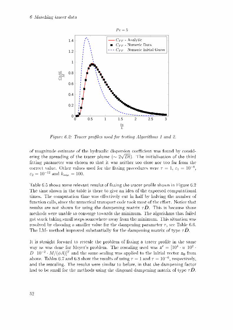
6 Matching tracer data
0 0.5 1 1.5 2 2.5 30
0.2
0.4
0.6
0.8
1
1.2
1.4
tuL
CφAL
M
Pe = 5
CFF - Analytic
CFF - Numeric Data
CFF - Numeric Initial Guess
Figure 6.2: Tracer pro�les used for testing Algorithms 1 and 2.
of magnitude estimate of the hydraulic dispersion coe�cient was found by consid-ering the spreading of the tracer plume (∼ 2
√Dt). The initialization of the third
�tting parameter was chosen so that it was neither too close nor too far from thecorrect value. Other values used for the �tting procedures were τ = 1, ε1 = 10−8,ε2 = 10−12 and kmax = 100.
Table 6.5 shows some relevant results of �tting the tracer pro�le shown in Figure 6.2The time shown in the table is there to give an idea of the expected computationaltimes. The computation time was e�ectively cut in half by halving the number offunction calls, since the numerical transport code took most of the e�ort. Notice thatresults are not shown for using the dampening matrix τD̂. This is because thosemethods were unable to converge towards the minimum. The algorithms that failedgot stuck taking small steps somewhere away from the minimum. This situation wasresolved by choosing a smaller value for the dampening parameter τ , see Table 6.6.The LM- method improved substantially for the dampening matrix of type τD̂.
It is straight forward to rescale the problem of �tting a tracer pro�le in the sameway as was done for Meyer's problem. The rescaling used was z′ = [104 · u 102 ·D 10−2 ·M/(φA)]T and the same scaling was applied to the initial vector z0 fromabove. Tables 6.7 and 6.8 show the results of using τ = 1 and τ = 10−6, respectively,and the rescaling. The results were similar to before, in that the dampening factorhad to be small for the methods using the diagonal dampening matrix of type τD̂.
52
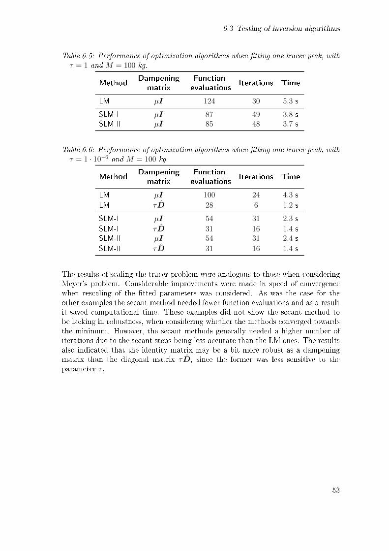
6.3 Testing of inversion algorithms
Table 6.5: Performance of optimization algorithms when �tting one tracer peak, withτ = 1 and M = 100 kg.
MethodDampening Function
Iterations Timematrix evaluations
LM µI 124 30 5.3 s
SLM-I µI 87 49 3.8 sSLM-II µI 85 48 3.7 s
Table 6.6: Performance of optimization algorithms when �tting one tracer peak, withτ = 1 · 10−6 and M = 100 kg.
MethodDampening Function
Iterations Timematrix evaluations
LM µI 100 24 4.3 s
LM τD̂ 28 6 1.2 s
SLM-I µI 54 31 2.3 s
SLM-I τD̂ 31 16 1.4 sSLM-II µI 54 31 2.4 s
SLM-II τD̂ 31 16 1.4 s
The results of scaling the tracer problem were analogous to those when consideringMeyer's problem. Considerable improvements were made in speed of convergencewhen rescaling of the �tted parameters was considered. As was the case for theother examples the secant method needed fewer function evaluations and as a resultit saved computational time. These examples did not show the secant method tobe lacking in robustness, when considering whether the methods converged towardsthe minimum. However, the secant methods generally needed a higher number ofiterations due to the secant steps being less accurate than the LM ones. The resultsalso indicated that the identity matrix may be a bit more robust as a dampeningmatrix than the diagonal matrix τD̂, since the former was less sensitive to theparameter τ .
53

6 Matching tracer data
Table 6.7: Performance of optimization algorithms when �tting one tracer peak, withscaled �tting parameters and τ = 1 · 100.
MethodDampening Function
Iterations Timematrix evaluations
LM µI 32 7 1.4 s
SLM-I µI 17 8 0.8 sSLM-II µI 17 8 0.8 s
Table 6.8: Performance of optimization algorithms when �tting one tracer peak, withscaled �tting parameters and τ = 1 · 10−6.
MethodDampening Function
Iterations Timematrix evaluations
LM µI 20 4 0.9 s
LM τD̂ 20 4 0.9 s
SLM-I µI 17 8 0.8 s
SLM-I τD̂ 17 8 0.8 sSLM-II µI 17 8 0.8 s
SLM-II τD̂ 17 8 0.8 s
54

7 Numerical experiments
Numerical experiments were conducted to look at di�erences between the tracermodels described in Chapters 3 and 5. Model predictions using the numerical pro-cedure outlined in Chapter 5 were compared to known analytical solutions to validatethe code implementing the numerical method.
7.1 Comparison of one-dimensional tracer models
Figures 3.10 and 3.11 show that the instantaneous injection solutions for one-dimensional �ow di�er quite a bit for small Peclet numbers. However, it is notapparent from those �gures how they compare when �tting tracer data. The instan-taneous solutions were compared by matching the pro�les to arti�cial tracer datacreated using the �ux-�ux solution, CFF .
The initial guess used for the �tting was z0 = [u0 D0 m0], where u0, D0 and m0
were the mean velocity, dispersion and injected mass, respectively, used for the CFFmodel. In the matching procedure, it was assumed that φA = q/u, i.e. the �ow rateq was kept constant. The e�ective cross-section, φA, was chosen this way because itis an unknown parameter in tracer testing but the �ow rate is known. The syntheticdata was generated for time intervals ∆t = L/(50u) from the injection time t = 0up to t = 3L/u.
Table 7.1 compares the �tted values of the models to the ones used for the CFF modelfor selected Peclet numbers. The predicted injection masses are almost identical forPe > 5, but the estimated dispersion and velocity parameters deviated quite a bitwith up to about 20% di�erence even at Pe = 10. The �tted pro�les themselvescompare fairly well for Pe & 5, see Figure 7.1. The lower plot in Figure 7.1 showshow the solutions with either detection or injection in resident concentration areunable to capture the shape of the �ux-�ux solution at small Peclet numbers. Theresidential concentration models underpredict the peak concentration as well as thetail of the �ux-�ux tracer pro�le.
The results show that the CRR solution gave, as expected, the worst �t to the CFF
55
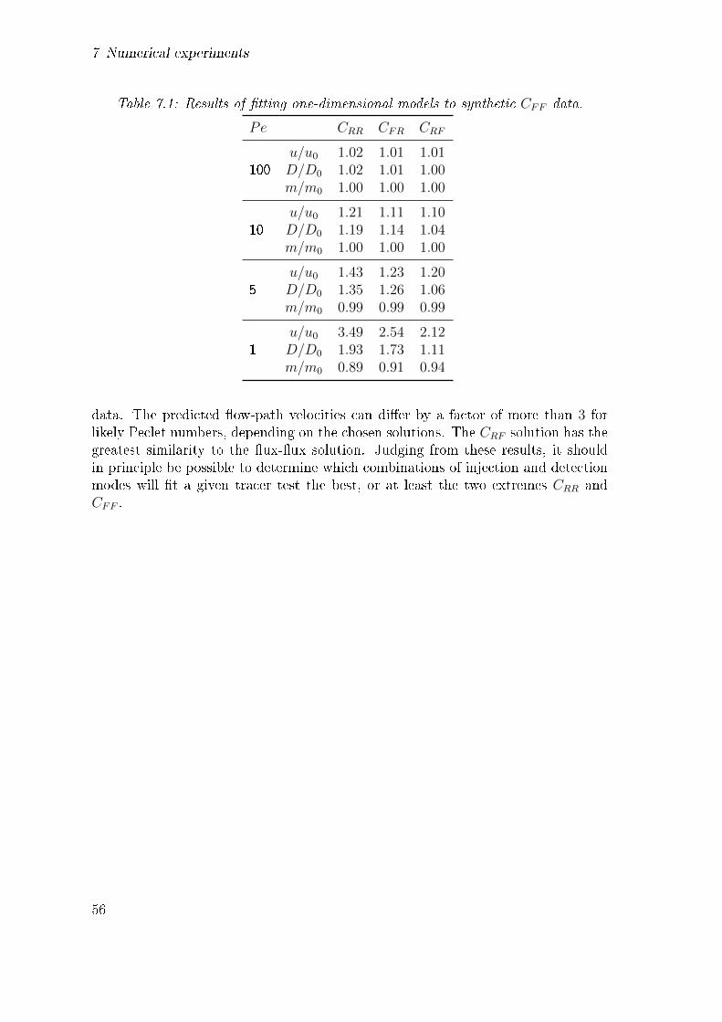
7 Numerical experiments
Table 7.1: Results of �tting one-dimensional models to synthetic CFF data.
Pe CRR CFR CRF
100u/u0 1.02 1.01 1.01D/D0 1.02 1.01 1.00m/m0 1.00 1.00 1.00
10u/u0 1.21 1.11 1.10D/D0 1.19 1.14 1.04m/m0 1.00 1.00 1.00
5u/u0 1.43 1.23 1.20D/D0 1.35 1.26 1.06m/m0 0.99 0.99 0.99
1u/u0 3.49 2.54 2.12D/D0 1.93 1.73 1.11m/m0 0.89 0.91 0.94
data. The predicted �ow-path velocities can di�er by a factor of more than 3 forlikely Peclet numbers, depending on the chosen solutions. The CRF solution has thegreatest similarity to the �ux-�ux solution. Judging from these results, it shouldin principle be possible to determine which combinations of injection and detectionmodes will �t a given tracer test the best, or at least the two extremes CRR andCFF .
56

7.1 Comparison of one-dimensional tracer models
0 0.5 1 1.5 2 2.5 30
0.2
0.4
0.6
0.8
1
tvL
CφAL
M
Pe = 5
CFF
CRR
CRF
CFR
0 0.5 1 1.5 2 2.5 30
0.2
0.4
0.6
0.8
1
1.2
1.4
tvL
CφALM
Pe = 1
CFF
CRR
CRF
CFR
Figure 7.1: Comparison of �tted one-dimensional instantaneous analytical solutionsto synthetically generated data using the solution with injection and detection in�ux concentration.
57
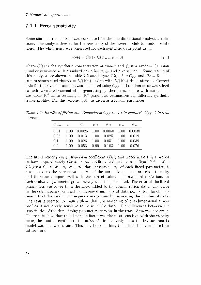
7 Numerical experiments
7.1.1 Error sensitivity
Some simple error analysis was conducted for the one-dimensional analytical solu-tions. The analysis checked for the sensitivity of the tracer models to random whitenoise. The white noise was generated for each synthetic data point using
noise = C(t) · fn(σnoise,µ = 0) (7.1)
where C(t) is the synthetic concentration at time t and fn is a random Gaussiannumber generator with standard deviation σnoise and a zero mean. Some results ofthis analysis are shown in Table 7.2 and Figure 7.2, using CFF and Pe = 5. Theresults shown used times t = L/(10u) : 4L/u with L/(10u) time intervals. Correctdata for the given parameters was calculated using CFF and random noise was addedto each calculated concentration generating synthetic tracer data with noise. Thiswas done 104 times resulting in 104 parameter estimations for di�erent synthetictracer pro�les. For this exercise φA was given as a known parameter.
Table 7.2: Results of �tting one-dimensional CFF model to synthetic CFF data withnoise.
σnoise µu σu µD σD µm σm
0.01 1.00 0.0026 1.00 0.0050 1.00 0.00380.05 1.00 0.013 1.00 0.025 1.00 0.0190.1 1.00 0.026 1.00 0.051 1.00 0.0390.2 1.00 0.053 0.99 0.103 1.00 0.076
The �tted velocity (u�t), dispersion coe�cient (D�t) and tracer mass (m�t) provedto have approximately Gaussian probability distributions, see Figure 7.2. Table7.2 gives the mean, µi, and standard deviation, σi, of each �tted parameter, i,normalized to the correct value. All of the normalized means are close to unityand therefore compare well with the correct value. The standard deviations foreach evaluated parameter grow linearly with the noise level. The error of the �ttedparameters was lower than the noise added to the concentration data. The errorin the estimations decreased for increased numbers of data points, for the obviousreason that the random noise gets averaged out by increasing the number of data.The results seemed to mainly show that the matching of one-dimensional tracerpro�les is not overly sensitive to noise in the data. The di�erences between thesensitivities of the three �tting parameters to noise in the tracer data was not great.The results show that the dispersion factor was the most sensitive, with the velocitybeing the least susceptible to the noise. A similar analysis for the fracture-matrixmodel was not carried out. This may be something that should be considered forfuture work.
58
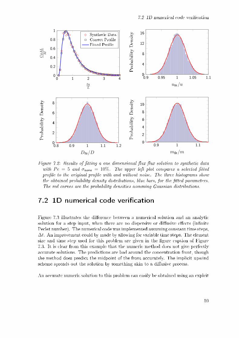
7.2 1D numerical code veri�cation
0 1 2 3 40
0.2
0.4
0.6
0.8
1
tuL
CφAL
M
Synthetic Data
Correct Pro�le
Fitted Pro�le
0.9 0.95 1 1.05 1.10
4
8
12
16
u�t/u
ProbabilityDensity
0.8 0.9 1 1.1 1.20
2
4
6
8
D�t/D
ProbabilityDensity
0.9 1 1.10
2
4
6
8
10
m�t/m
ProbabilityDensity
Figure 7.2: Results of �tting a one-dimensional �ux-�ux solution to synthetic datawith Pe = 5 and σnoise = 10%. The upper left plot compares a selected �ttedpro�le to the original pro�le with and without noise. The three histograms showthe obtained probability density distributions, blue bars, for the �tted parameters.The red curves are the probability densities assuming Gaussian distributions.
7.2 1D numerical code veri�cation
Figure 7.3 illustrates the di�erence between a numerical solution and an analyticsolution for a step input, when there are no dispersive or di�usive e�ects (in�nitePeclet number). The numerical code was implemented assuming constant time steps,∆t. An improvement could by made by allowing for variable time steps. The elementsize and time step used for this problem are given in the �gure caption of Figure7.3. It is clear from this example that the numeric method does not give perfectlyaccurate solutions. The predictions are bad around the concentration front, thoughthe method does predict the midpoint of the front accurately. The implicit upwindscheme spreads out the solution by something akin to a di�usive process.
An accurate numeric solution to this problem can easily be obtained using an explcit
59

7 Numerical experiments
0 0.2 0.4 0.6 0.8 1 1.2 1.4 1.6 1.8 2
0
0.2
0.4
0.6
0.8
1
tuL
C/C
I
CCFF - Analytic
Numeric
Figure 7.3: Comparison of one-dimensional numerical and analytical solutions forthe case of pure advection and continuous injection at constant concentration, CI .The numerical solution shown used elements of constant length ∆x = L/100 anda time step ∆t = ∆x/u.
�nite di�erence scheme. The transport equation for this problem is
∂C
∂t+ u
∂C
∂x= 0 . (7.2)
For an explicit �nite di�erence method this equation can be written as
CP − C0P
∆t+ u
C0P − C0
W
∆x= 0 . (7.3)
Rearranging givesCP = C0
P · (1− Cr) + Cr · C0W , (7.4)
where Cr = u∆t/∆x is the Courant number. An exact solution for the problembeing discussed is found by choosing Cr = 1. The Courant number is an importantparameter when considering the stability of explicit schemes. Cr ≤ 1 is usually anecessary criterion for the numerical stability of one-dimensional explicit schemes.The physical explanation is that convective information may not travel further thanthe distance between neighbouring nodes during a given time step.
The implicit upwind scheme is still the method of choice for this work due to itsrobustness and stability for large time steps. The numerical inaccuracy incurred by
60
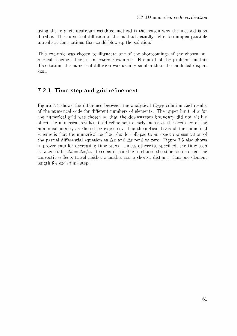
7.2 1D numerical code veri�cation
using the implicit upstream weighted method is the reason why the method is sodurable. The numerical di�usion of the method actually helps to dampen possibleunrealistic �uctuations that could blow up the solution.
This example was chosen to illustrate one of the shortcomings of the chosen nu-merical scheme. This is an extreme example. For most of the problems in thisdissertation, the numerical di�usion was usually smaller than the modelled disper-sion.
7.2.1 Time step and grid re�nement
Figure 7.4 shows the di�erence between the analytical CCFF solution and resultsof the numerical code for di�erent numbers of elements. The upper limit of x forthe numerical grid was chosen so that the downstream boundary did not visiblya�ect the numerical results. Grid re�nement clearly increases the accuracy of thenumerical model, as should be expected. The theoretical basis of the numericalscheme is that the numerical method should collapse to an exact representation ofthe partial di�erential equation as ∆x and ∆t tend to zero. Figure 7.5 also showsimprovements for decreasing time steps. Unless otherwise speci�ed, the time stepis taken to be ∆t = ∆x/u. It seems reasonable to choose the time step so that theconvective e�ects travel neither a further nor a shorter distance than one elementlength for each time step.
61

7 Numerical experiments
0 0.2 0.4 0.6 0.8 1 1.2 1.4 1.6 1.8 20
0.2
0.4
0.6
0.8
1
tuL
C/C
I
Pe = 100
CCFF - Analytic
Numeric ∆x = L/50
Numeric ∆x = L/100
Numeric ∆x = L/200
0 0.2 0.4 0.6 0.8 1 1.2 1.4 1.6 1.8 2
−0.1
0
0.1
tuL
(C−CCFF
)/CI
Pe = 100
Numeric ∆x = L/50
Numeric ∆x = L/100
Numeric ∆x = L/200
Figure 7.4: Comparison of one-dimensional numerical and analytical solutions forthe case of continuous injection at constant �ux concentration, CI , and detectionin �ux, when Pe = 100. The numerical solutions shown employed constant timesteps ∆t = ∆x/u. The lower image shows the relative di�erence between the nu-merical and analytical solutions. Grid re�nement clearly improves the numericalsolution.
62

7.2 1D numerical code veri�cation
0 0.2 0.4 0.6 0.8 1 1.2 1.4 1.6 1.8 20
0.2
0.4
0.6
0.8
1
tuL
C/C
IPe = 100
CCFF - Analytic
Numeric ∆t = 2∆x/u
Numeric ∆t = ∆x/u
Numeric ∆t = 12∆x/u
0 0.2 0.4 0.6 0.8 1 1.2 1.4 1.6 1.8 2
−0.1
0
0.1
0.2
tuL
(C−CCFF
)/CI
Pe = 100
Numeric ∆t = 2∆x/u
Numeric ∆t = ∆x/u
Numeric ∆t = 12∆x/u
Figure 7.5: Comparison of one-dimensional numerical and analytical solutions forthe case of continuous injection at constant �ux concentration, CI , and detectionin �ux, when Pe = 100. The numerical solutions shown used a constant elementsize of ∆x = L/50. The lower image shows the relative di�erence between thenumerical and analytical solutions.
63

7 Numerical experiments
7.2.2 Numerical di�usion
The problem of numerical di�usion has already been touched on. The implicitupstream weighted scheme used for solving the one-dimensional advection dispersionequation induces numerical dispersion which has an e�ective dispersion coe�cient
Dnum ≈u∆x
2(1 + Cr) (7.5)
(Peaceman, 1977). This numerical dispersion or di�usion coe�cient is reduced withgrid and time step re�nement.
Figure 7.6 compares the di�erence between the usual numerical solution, which usesD = uL/Pe, and a solution using a corrected dispersion coe�cient D −Dnum. Thecorrected numerical method gives results which are a very good approximation tothe analytical solution. For the case in point the corrected dispersion coe�cient wasequal to zero. Care needs to be taken not to correct the dispersion too much, sincea negative dispersion coe�cient can make the numerical method unstable and couldresult in physically unrealistic values.
Figure 7.7 compares CFF solutions found using numerical and analytical methods.The input boundary condition used for instantaneous injection in �ux of mass mwas
uCI =
{u ·m/(q∆t) , if 0 ≤ t < ∆t
0 , else(7.6)
The numerical results compared reasonably well with the analytical solution, seeFigure 7.7. The method using the dispersion correction performed better, even whenre�ning the grid and time steps. The correction to the dispersion factor proved tohelp increase the accuracy of the results.
64
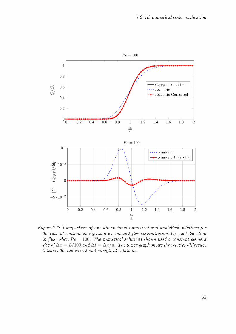
7.2 1D numerical code veri�cation
0 0.2 0.4 0.6 0.8 1 1.2 1.4 1.6 1.8 20
0.2
0.4
0.6
0.8
1
tuL
C/C
IPe = 100
CCFF - Analytic
Numeric
Numeric Corrected
0 0.2 0.4 0.6 0.8 1 1.2 1.4 1.6 1.8 2
−5 · 10−2
0
5 · 10−2
0.1
tuL
(C−CCFF
)/CI
Pe = 100
Numeric
Numeric Corrected
Figure 7.6: Comparison of one-dimensional numerical and analytical solutions forthe case of continuous injection at constant �ux concentration, CI , and detectionin �ux, when Pe = 100. The numerical solutions shown used a constant elementsize of ∆x = L/100 and ∆t = ∆x/u. The lower graph shows the relative di�erencebetween the numerical and analytical solutions.
65
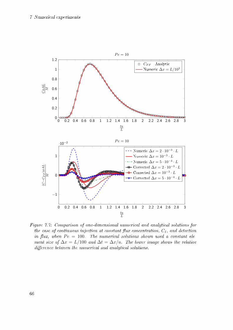
7 Numerical experiments
0 0.2 0.4 0.6 0.8 1 1.2 1.4 1.6 1.8 2 2.2 2.4 2.6 2.8 30
0.2
0.4
0.6
0.8
1
1.2
tuL
CφAL
M
Pe = 10
CFF - Analytic
Numeric ∆x = L/103
0 0.2 0.4 0.6 0.8 1 1.2 1.4 1.6 1.8 2 2.2 2.4 2.6 2.8 3
−1
0
1
·10−2
tuL
(C−CFF
)φAL
M
Pe = 10
Numeric ∆x = 2 · 10−3 · LNumeric ∆x = 10−3 · LNumeric ∆x = 5 · 10−4 · LCorrected ∆x = 2 · 10−3 · LCorrected ∆x = 10−3 · LCorrected ∆x = 5 · 10−4 · L
Figure 7.7: Comparison of one-dimensional numerical and analytical solutions forthe case of continuous injection at constant �ux concentration, CI , and detectionin �ux, when Pe = 100. The numerical solutions shown used a constant ele-ment size of ∆x = L/100 and ∆t = ∆x/u. The lower image shows the relativedi�erence between the numerical and analytical solutions.
66

7.2 1D numerical code veri�cation
Implementing the corrected dispersion coe�cient is trivial when the resident con-centration is the observed output. This is not the case when the the productionis measured in �ux. Without a correction, the numerically calculated �ux concen-tration is given by equation (5.22). If a corrected dispersion coe�cient is used,it is possible that the following incorrect equation is used for the produced �uxconcentration:
Ce −D
u
∂C
∂x
∣∣∣∣e
≈ CL+ − D −Dnum
u
CL+ − CL−
δxw(7.7)
The above �ux concentration is being evaluated at the production boundary locatedat x = L. The subscripts L+ and L− denote calculated resident concentrations ofthe closest upstream and downstream elements, respectively. This is incorrect whenthe modelled variable is the resident concentration, because the numerical dispersionbeing corrected for, shows itself in the calculated concentrations, Ci, but not thefactor D/u. This confusion may be avoided by choosing the �ux concentration itselfas the modelled variable. This is not done here since the fracture-matrix model needsthe resident concentration at the fracture-matrix interface, and chemical reactionsare usually in terms of the resident concentration not �ux concentration. Figure7.8 compares the numerical error, for the same curve as shown in Figure 7.7, whenusing the correct and the incorrect method of accounting for numerical di�usion.The proper version resulted in a better curve than the one found using the incorrectmethod.
0 0.2 0.4 0.6 0.8 1 1.2 1.4 1.6 1.8 2 2.2 2.4 2.6 2.8 3
−1
−0.5
0
0.5
·10−2
tuL
(C−CFF
)φAL
M
Pe = 10
Corrected ∆x = 2 · 10−3 · LImproper Adjustment ∆x = 2 · 10−3 · L
Figure 7.8: Improper and proper adjustment to account for numerical di�usion,considering numerical di�usion. When calculating the outward �ux D should beused instead of D −Dnum.
67
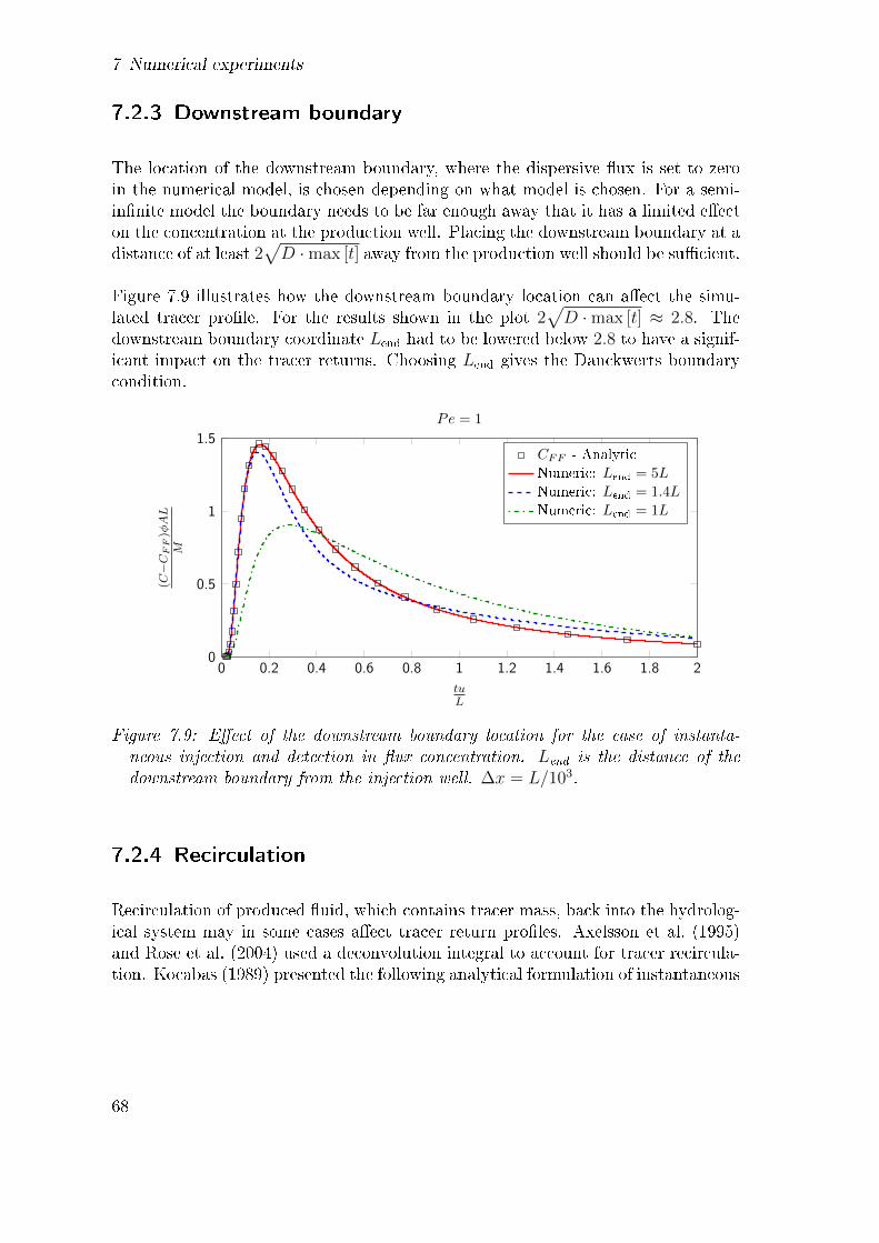
7 Numerical experiments
7.2.3 Downstream boundary
The location of the downstream boundary, where the dispersive �ux is set to zeroin the numerical model, is chosen depending on what model is chosen. For a semi-in�nite model the boundary needs to be far enough away that it has a limited e�ecton the concentration at the production well. Placing the downstream boundary at adistance of at least 2
√D ·max [t] away from the production well should be su�cient.
Figure 7.9 illustrates how the downstream boundary location can a�ect the simu-lated tracer pro�le. For the results shown in the plot 2
√D ·max [t] ≈ 2.8. The
downstream boundary coordinate Lend had to be lowered below 2.8 to have a signif-icant impact on the tracer returns. Choosing Lend gives the Danckwerts boundarycondition.
0 0.2 0.4 0.6 0.8 1 1.2 1.4 1.6 1.8 20
0.5
1
1.5
tuL
(C−CFF
)φAL
M
Pe = 1
CFF - Analytic
Numeric: Lend = 5L
Numeric: Lend = 1.4L
Numeric: Lend = 1L
Figure 7.9: E�ect of the downstream boundary location for the case of instanta-neous injection and detection in �ux concentration. Lend is the distance of thedownstream boundary from the injection well. ∆x = L/103.
7.2.4 Recirculation
Recirculation of produced �uid, which contains tracer mass, back into the hydrolog-ical system may in some cases a�ect tracer return pro�les. Axelsson et al. (1995)and Rose et al. (2004) used a deconvolution integral to account for tracer recircula-tion. Kocabas (1989) presented the following analytical formulation of instantaneous
68
7.2 1D numerical code veri�cation
reinjection of all the produced tracer:
CFF (L, t) =m
q
∞∑n=0
(n+ 1)L
2√πDt3
exp
[−((n+ 1)L− ut)2
4Dt
](7.8)
The injection and detection are in �ux concentration. Boundary and initial condi-tions are
CF (x, 0) = 0 , CF (0, t) =m
qδ(t) + CF (L, t) and lim
x→∞CF (x, t) = 0 (7.9)
The model is equivalent to a solution where a tracer mass m is injected into theone-dimensional system at time t = 0 at points where x ≤ 0 and the remainder ofx/L is zero (injection of tracer mass m at L intervals for x ≤ 0). This model canbe adjusted to account for situations where reinjected �uid is mixed with �uid fromanother source. Assuming the mixing �uid then
CFF (L, t) =M
QP
∞∑n=0
ωn+1inj ω
nreinj
(n+ 1)L
2√πDt3
exp
[−((n+ 1)L− ut)2
4Dt
](7.10)
where ωreinj is the fraction of injection �uid coming from the production well. Thiscan easily be generalized for modelling of multiple �ow-channels. Accounting forreinjection becomes involved, if the injection �uid springs from multiple productionwells producing �uid containing tracers. However, a numerical model could in prac-tice solve such a recirculation problem by coupling the tracer production models formultiple production wells.
To account for reinjection in the numerical simulation code the following equationwas used
Φw(t) = Φinitial(t) +ωinj ·ωreinj ·Φprod(t) = Φinitial(t) +ωinj ·ωreinj · uCFF (L, t) (7.11)
Here it has been assumed that the injected tracer mass into the channel is m =ωinjM . CPF is the �ux concentration at the production well. Figure 7.11 showsa comparison of using the analytical equation describing recirculation and the nu-merical code employing equation (7.11). The �gure illustrates both recirculation ofall the tracer (ωinj · ωreinj = 1) and partial recirculation (ωinj · ωreinj < 1). The twosolution methods show good agreement. The normalized concentration, CφAL/M ,tends to unity for late times, in concurrence with equation (3.52). If the reinjectionof production water does not occur instantaneously then equation (7.11) becomes
Φw(t) = Φinitial(t) + ωinj · ωreinj · uCFF (L, t− td) (7.12)
where td is the pipeline delay time (time it takes the produced �uid to be reinjected).
69

7 Numerical experiments
0 0.5 1 1.5 2 2.5 3 3.5 4 4.5 50
1
2
3
tuL
CφAL
M
Pe = 100
Analytic: 100% recirculation
Numeric: 100% recirculation
Analytic: 50% recirculation
Numeric: 50% recirculation
0 0.5 1 1.5 2 2.5 3 3.5 4 4.5 50
0.5
1
tuL
CφAL
M
Pe = 10
Analytic: 100% recirculation
Numeric: 100% recirculation
Analytic: 20% recirculation
Numeric: 20% recirculation
Analytic: 0% recirculation
Numeric: 0% recirculation
0 0.5 1 1.5 2 2.5 3 3.5 4 4.5 50
0.5
1
1.5
tuL
CφAL
M
Pe = 1
Analytic: 100% recirculation
Numeric: 100% recirculation
Analytic: 20% recirculation
Numeric: 20% recirculation
Analytic: 0% recirculation
Numeric: 0% recirculation
Figure 7.10: Numerical and analytical solutions of the recirculation problem, fordi�erent recirculation fractions, ωinj ·ωreinj. The numerical code used ∆x = L/103.
70
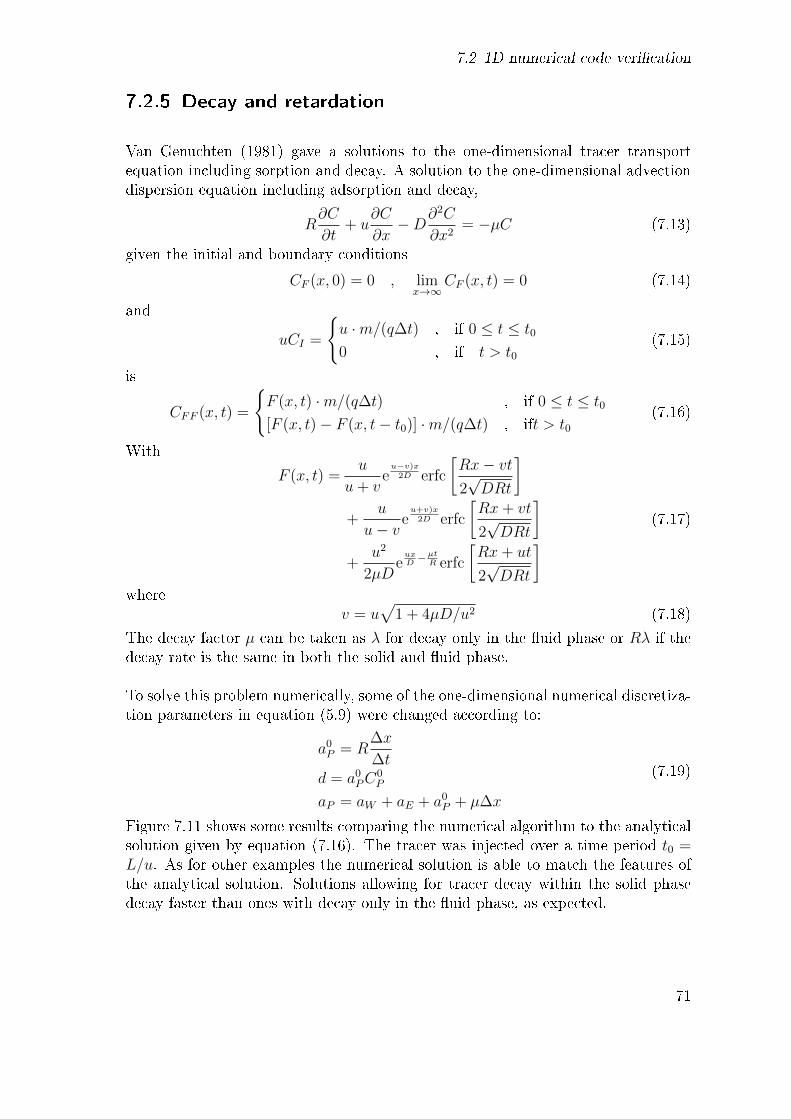
7.2 1D numerical code veri�cation
7.2.5 Decay and retardation
Van Genuchten (1981) gave a solutions to the one-dimensional tracer transportequation including sorption and decay. A solution to the one-dimensional advectiondispersion equation including adsorption and decay,
R∂C
∂t+ u
∂C
∂x−D∂
2C
∂x2= −µC (7.13)
given the initial and boundary conditions
CF (x, 0) = 0 , limx→∞
CF (x, t) = 0 (7.14)
and
uCI =
{u ·m/(q∆t) , if 0 ≤ t ≤ t0
0 , if t > t0(7.15)
is
CFF (x, t) =
{F (x, t) ·m/(q∆t) , if 0 ≤ t ≤ t0
[F (x, t)− F (x, t− t0)] ·m/(q∆t) , ift > t0(7.16)
With
F (x, t) =u
u+ veu−v)x2D erfc
[Rx− vt2√DRt
]+
u
u− veu+v)x2D erfc
[Rx+ vt
2√DRt
]+
u2
2µDeuxD−µtR erfc
[Rx+ ut
2√DRt
] (7.17)
wherev = u
√1 + 4µD/u2 (7.18)
The decay factor µ can be taken as λ for decay only in the �uid phase or Rλ if thedecay rate is the same in both the solid and �uid phase.
To solve this problem numerically, some of the one-dimensional numerical discretiza-tion parameters in equation (5.9) were changed according to:
a0P = R
∆x
∆td = a0
PC0P
aP = aW + aE + a0P + µ∆x
(7.19)
Figure 7.11 shows some results comparing the numerical algorithm to the analyticalsolution given by equation (7.16). The tracer was injected over a time period t0 =L/u. As for other examples the numerical solution is able to match the features ofthe analytical solution. Solutions allowing for tracer decay within the solid phasedecay faster than ones with decay only in the �uid phase, as expected.
71
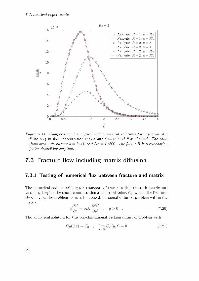
7 Numerical experiments
0 0.5 1 1.5 2 2.5 3 3.5 40
2
4
6
8
10
12
14
16·10−2
tuL
CφAL
m
Pe = 3
Analytic: R = 1, µ = Rλ
Numeric: R = 1, µ = Rλ
Analytic: R = 2, µ = λ
Numeric: R = 2, µ = λ
Analytic: R = 2, µ = Rλ
Numeric: R = 2, µ = Rλ
Figure 7.11: Comparison of analytical and numerical solutions for injection of a�nite slug in �ux concentration into a one-dimensional �ow-channel. The solu-tions used a decay rate λ = 2u/L and ∆x = L/500. The factor R is a retardationfactor describing sorption.
7.3 Fracture �ow including matrix di�usion
7.3.1 Testing of numerical �ux between fracture and matrix
The numerical code describing the transport of tracers within the rock matrix wastested by keeping the tracer concentration at constant value, C0, within the fracture.By doing so, the problem reduces to a one-dimensional di�usion problem within thematrix:
φ∂C
∂t= φDm
∂2C
∂y2, y > 0 . (7.20)
The analytical solution for this one-dimensional Fickian di�usion problem with
CR(0, t) = C0 , limy→∞
CF (y, t) = 0 (7.21)
72
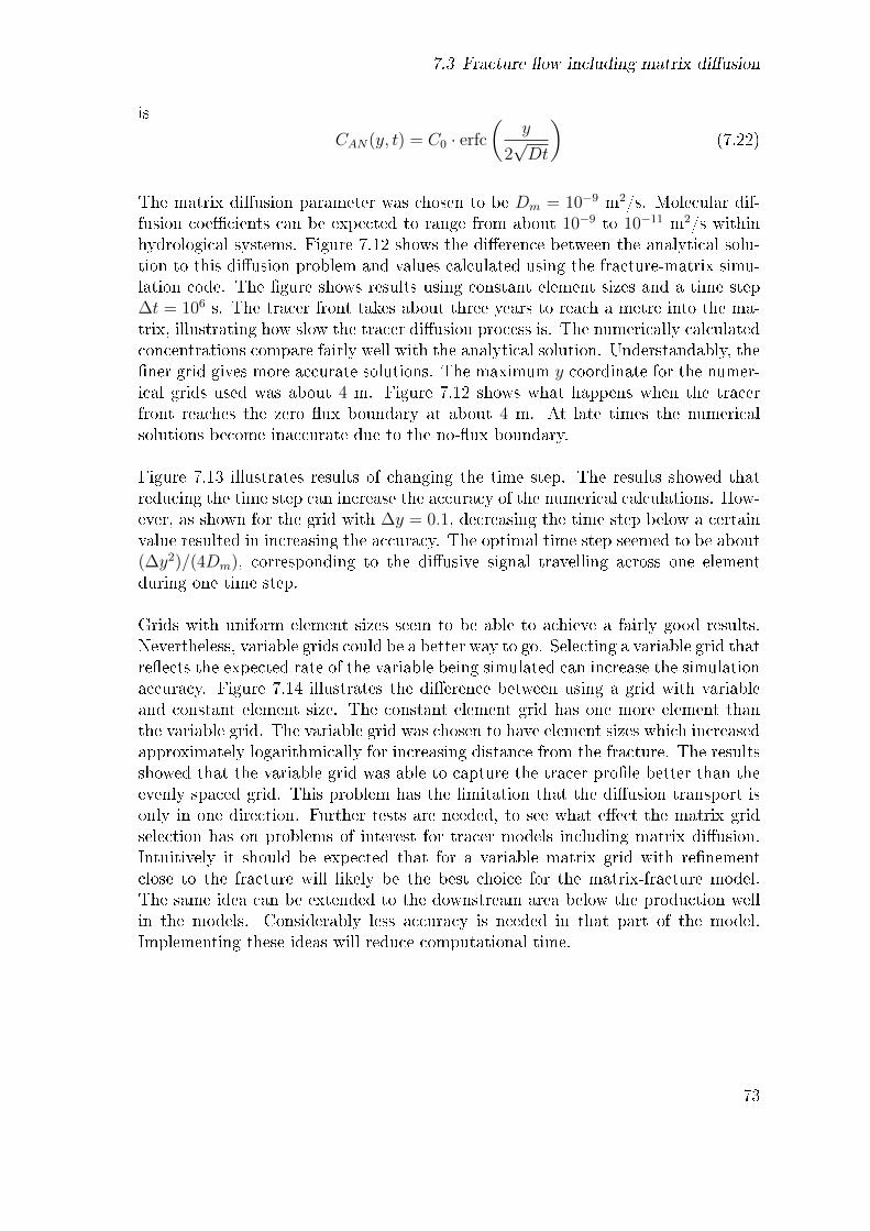
7.3 Fracture �ow including matrix di�usion
is
CAN(y, t) = C0 · erfc
(y
2√Dt
)(7.22)
The matrix di�usion parameter was chosen to be Dm = 10−9 m2/s. Molecular dif-fusion coe�cients can be expected to range from about 10−9 to 10−11 m2/s withinhydrological systems. Figure 7.12 shows the di�erence between the analytical solu-tion to this di�usion problem and values calculated using the fracture-matrix simu-lation code. The �gure shows results using constant element sizes and a time step∆t = 106 s. The tracer front takes about three years to reach a metre into the ma-trix, illustrating how slow the tracer di�usion process is. The numerically calculatedconcentrations compare fairly well with the analytical solution. Understandably, the�ner grid gives more accurate solutions. The maximum y coordinate for the numer-ical grids used was about 4 m. Figure 7.12 shows what happens when the tracerfront reaches the zero �ux boundary at about 4 m. At late times the numericalsolutions become inaccurate due to the no-�ux boundary.
Figure 7.13 illustrates results of changing the time step. The results showed thatreducing the time step can increase the accuracy of the numerical calculations. How-ever, as shown for the grid with ∆y = 0.1, decreasing the time step below a certainvalue resulted in increasing the accuracy. The optimal time step seemed to be about(∆y2)/(4Dm), corresponding to the di�usive signal travelling across one elementduring one time step.
Grids with uniform element sizes seem to be able to achieve a fairly good results.Nevertheless, variable grids could be a better way to go. Selecting a variable grid thatre�ects the expected rate of the variable being simulated can increase the simulationaccuracy. Figure 7.14 illustrates the di�erence between using a grid with variableand constant element size. The constant element grid has one more element thanthe variable grid. The variable grid was chosen to have element sizes which increasedapproximately logarithmically for increasing distance from the fracture. The resultsshowed that the variable grid was able to capture the tracer pro�le better than theevenly spaced grid. This problem has the limitation that the di�usion transport isonly in one direction. Further tests are needed, to see what e�ect the matrix gridselection has on problems of interest for tracer models including matrix di�usion.Intuitively it should be expected that for a variable matrix grid with re�nementclose to the fracture will likely be the best choice for the matrix-fracture model.The same idea can be extended to the downstream area below the production wellin the models. Considerably less accuracy is needed in that part of the model.Implementing these ideas will reduce computational time.
73

7 Numerical experiments
10−2 10−1 1000
0.2
0.4
0.6
0.8
1
y [m]
C/C
0
t = 107 s
41 Elements
81 Elements
10−2 10−1 100
−2
0
·10−2
y [m]
(C−CAN
)/C
0
t = 107 s
41 Elements
81 Elements
10−2 10−1 1000
0.2
0.4
0.6
0.8
1
y [m]
C/C
0
t = 108 s
41 Elements
81 Elements
10−2 10−1 100
−2
0
2·10−3
y [m]
(C−CAN
)/C
0
t = 108 s
41 Elements
81 Elements
10−2 10−1 1000
0.2
0.4
0.6
0.8
1
y [m]
C/C
0
t = 1010 s
41 Elements
81 Elements
10−2 10−1 1000
0.1
0.2
0.3
0.4
y [m]
(C−CAN
)/C
0
t = 1010 s
41 Elements
81 Elements
Figure 7.12: Numerical results compared with the analytical solution (black curve)for one-dimensional di�usion with a constant concentration boundary, equation(7.22). The numerical solutions shown used equally spaced elements with ∆y =0.1 m (red circles) and ∆y = 0.05 m (blue triangles).
74
7.3 Fracture �ow including matrix di�usion
10−2 10−1 100
0
0.5
1
1.5
·10−2
y [m]
(C−CAN
)/C
0
t = 108 s
41 Elements: ∆t = 107 s
81 Elements: ∆t = 107 s
41 :lements ∆t = 106 s
81 Elements ∆t = 106 s
41 Elements ∆t = 105 s
81 Elements ∆t = 105 s
Figure 7.13: Di�erence between the analytical solution of the one-dimensional di�u-sion problem and numerical solutions, for di�erent numbers of elements and timesteps, ∆t. The solution using 41 elements used ∆y = 0.1 m but the one using 81elements had elements half that size.
75

7 Numerical experiments
10−2 10−1 1000
0.2
0.4
0.6
0.8
1
y [m]
C/C
0
t = 108 s
Analytic solution: CAN
81 Elements: Constant element size
80 Elements: Variable element size
10−2 10−1 100−0.5
0
0.5
1
1.5·10−3
y [m]
(C−CAN
)/C
0
t = 108 s
81 Elements: Constant element size
80 Elements: Variable element size
Figure 7.14: Results of modelling one-dimensional matrix di�usion. The resultsillustrate how a variable grid can improve modelling results.
76

7.3 Fracture �ow including matrix di�usion
7.3.2 Fracture-matrix model
Figure 7.15 shows the di�erence between using a variable element size in the matrixand �xed element size. The numerical experiment compared the analytical solutionto a fracture-matrix system given by equation (3.62) and numerical simulationsfor the same boundary conditions. The simulations used similar parameters tothe estimated values used by Maloszewski et al. (1999) for their modelling andinterpretation of tracer tests carried out in the Lange Bramke basin, Germany. Thesimulations used Q = 10−3 m3/s, t0 = 0.85 days, m = 10 kg, L = 200 m, Pe = 6.9,a = 4.32 · 10−3 s−1/2, Dm = 10−9 m2/s and φm = 0.01. The numerical models used∆x = L/100 and about 2 · 104 elements.
The results showed that choosing variable sized elements can improve the numericalcalculations. The reason for using the variable sized grid approach is that it allowsfor greater accuracy in places where the tracer concentration changes most rapidly.For the fracture-matrix model the grid needs to be re�ned close to the fracture tocapture the fracture-matrix interaction. Both numerical models overestimated thetracer concentration at early times and underestimated the peak concentration.
77
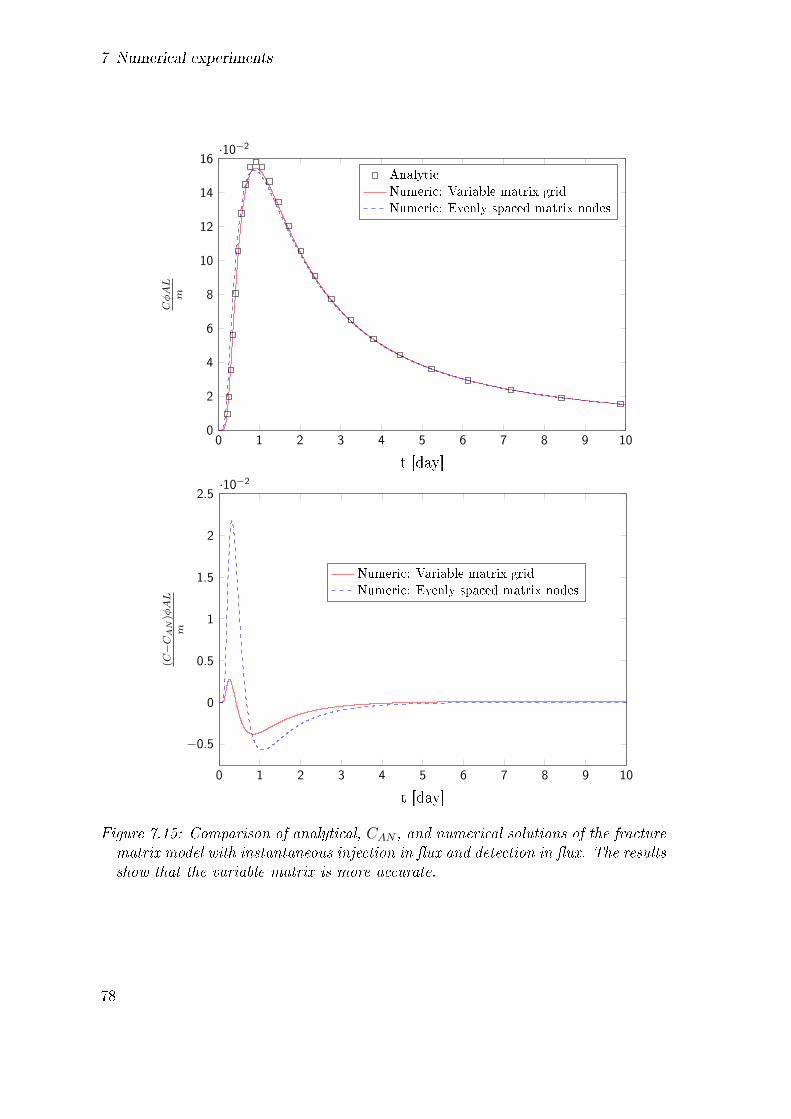
7 Numerical experiments
0 1 2 3 4 5 6 7 8 9 100
2
4
6
8
10
12
14
16·10−2
t [day]
CφAL
mAnalytic
Numeric: Variable matrix grid
Numeric: Evenly spaced matrix nodes
0 1 2 3 4 5 6 7 8 9 10
−0.5
0
0.5
1
1.5
2
2.5·10−2
t [day]
(C−CAN
)φAL
m
Numeric: Variable matrix grid
Numeric: Evenly spaced matrix nodes
Figure 7.15: Comparison of analytical, CAN , and numerical solutions of the fracturematrix model with instantaneous injection in �ux and detection in �ux. The resultsshow that the variable matrix is more accurate.
78

8 Soda Lake tracer test
A tracer test �eld experiment using sorbing and conservative tracers was conductedin the autumn of 2011 in the Soda Lake geothermal �eld, Nevada, USA. Detailsof the experiment can by found in Rose et al. (2012) and Williams et al. (2013).Reimus et al. (2012) and Williams et al. (2013) discussed results of analysing thetracer returns from the experiment. They used the semi-analytical RELAP modelfor history matching of the measured tracer responses.
Figure 8.1: Illustration of the Soda Lake tracer test (Williams et al., 2013).
On the eighth of August, 2011, 50 kg of 1,6-naphthalene disulfonate (1,6-NDS)and 90 kg of Safranin-T (Saf-T) were injected into well 45A-33. Subsequent tracerreturns were monitored at well 32-33 for the following 28 days. The 1,6-NDS wasinjected during the �rst half hour of the test and the Saf-T was injected over the nextthree hours, due to di�culties with injection (Reimus et al., 2012). The separationof the two wells is approximately L = 550 m. The NDS tracer was thermally stableand conservative but the Safranin tracer thermally degraded and sorbed within the�eld. A constant injection rate of about 55.5 L/s (880 gpm) was maintained at well
79

8 Soda Lake tracer test
45A-33 and about 55.8 L/s (885 gpm) were continuously produced from well 32-33,see Figure 8.1. Around 26.5% of the �uid produced at well 32-33 was reinjectedback into well 45A-33. The temperature of the injection �uid was 70◦C and theproduced �uid had a temperature of 190◦C.
8.1 Thermal decay of Safranin-T
Rose et al. (2012) measured the temperature dependence of the Safranin-T decayrate using autoclave batch reactors for a temperature range of 160-190◦C. Rose et al.(2001) describe the details of the measurement technique used. They modelled thethermal decay reaction kinetics assuming a �rst order decay rate:
∂CS∂t
= −λSCS (8.1)
where CS is the Safranin-T concentration. The temperature dependence of the Saf-Tdecay rate, λS, can be described using an Arrhenius relation:
λS = A e− EaRgT (8.2)
where Rg is the gas constant, A is some pre-exponential factor, Ea is the activationenergy and T is the absolute temperature.
Rose et al. (2012) found the following empirical relation for the Saf-T decay rate:
ln (λS) = 24.3− 11500T−1 (8.3)
with the decay rate in inverse days (day−1).
8.2 Analysis of tracer data
Figure 8.2 shows the measured tracer concentrations. Reimus et al. (2012), Roseet al. (2012) and Williams et al. (2013) corrected the Saf-T data for thermal degra-dation assuming a 180◦C e�ective interwell temperature and a decay rate in thesolid phase equal to the rate in the �uid. This should be a good assumption, sinceinjection into well 45A-33 had not been long enough to result in signi�cant cooling(Rose et al., 2012). Table 8.1 shows some results found using RELAP to matchthe tracer data using a zero matrix di�usion model and a double-porosity model.RELAP uses the same boundary conditions as Maloszewski and Zuber (1990) andaccounts for fracture and matrix retardation.
80
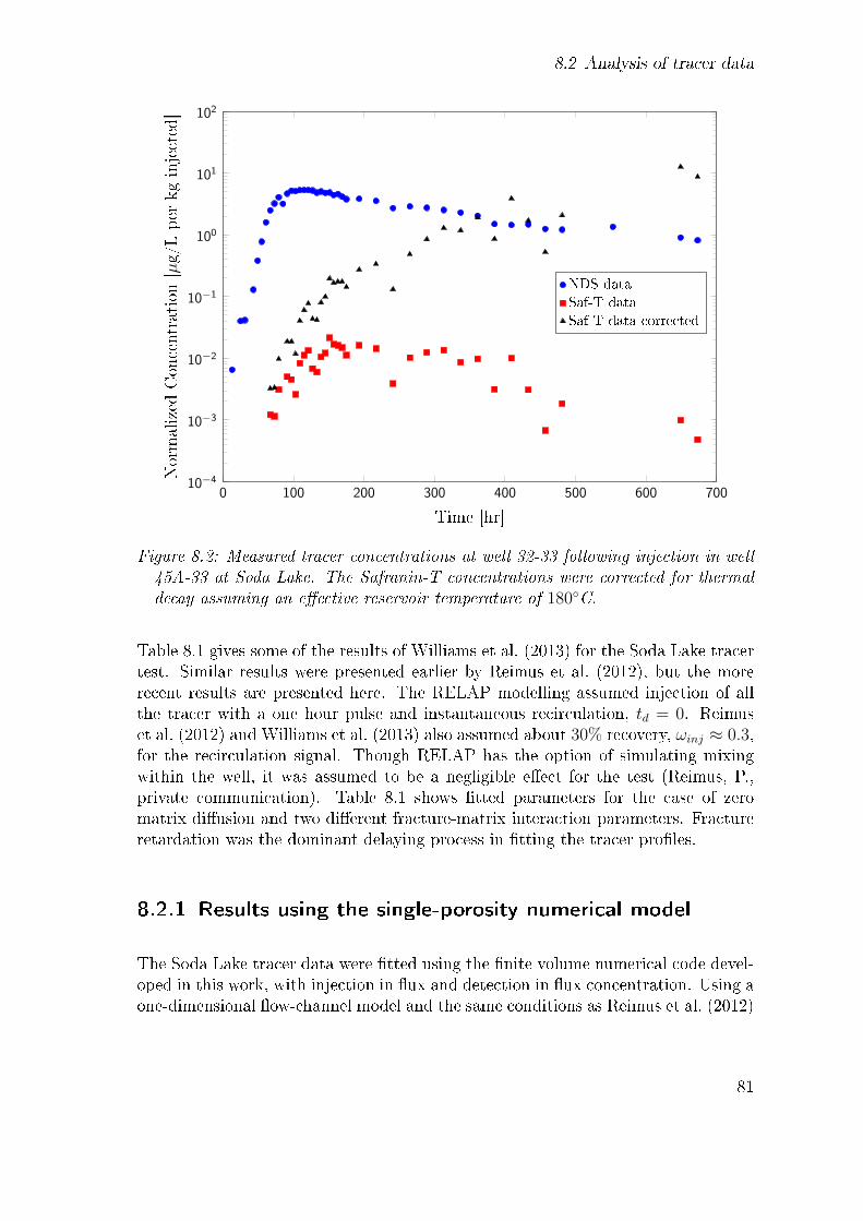
8.2 Analysis of tracer data
0 100 200 300 400 500 600 70010−4
10−3
10−2
10−1
100
101
102
Time [hr]
Normalized
Concentration
[µg/Lper
kginjected]
NDS data
Saf-T data
Saf-T data corrected
Figure 8.2: Measured tracer concentrations at well 32-33 following injection in well45A-33 at Soda Lake. The Safranin-T concentrations were corrected for thermaldecay assuming an e�ective reservoir temperature of 180◦C.
Table 8.1 gives some of the results of Williams et al. (2013) for the Soda Lake tracertest. Similar results were presented earlier by Reimus et al. (2012), but the morerecent results are presented here. The RELAP modelling assumed injection of allthe tracer with a one hour pulse and instantaneous recirculation, td = 0. Reimuset al. (2012) and Williams et al. (2013) also assumed about 30% recovery, ωinj ≈ 0.3,for the recirculation signal. Though RELAP has the option of simulating mixingwithin the well, it was assumed to be a negligible e�ect for the test (Reimus, P.,private communication). Table 8.1 shows �tted parameters for the case of zeromatrix di�usion and two di�erent fracture-matrix interaction parameters. Fractureretardation was the dominant delaying process in �tting the tracer pro�les.
8.2.1 Results using the single-porosity numerical model
The Soda Lake tracer data were �tted using the �nite volume numerical code devel-oped in this work, with injection in �ux and detection in �ux concentration. Using aone-dimensional �ow-channel model and the same conditions as Reimus et al. (2012)
81
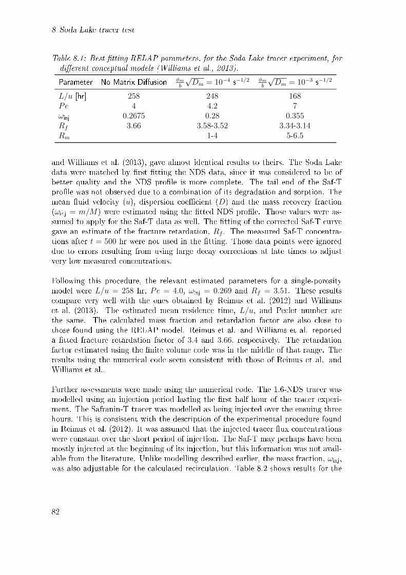
8 Soda Lake tracer test
Table 8.1: Best �tting RELAP parameters, for the Soda Lake tracer experiment, fordi�erent conceptual models (Williams et al., 2013).
Parameter No Matrix Di�usion φmb
√Dm = 10−4 s−1/2 φm
b
√Dm = 10−3 s−1/2
L/u [hr] 258 248 168Pe 4 4.2 7ωinj 0.2675 0.28 0.355Rf 3.66 3.58-3.52 3.34-3.14Rm 1-4 5-6.5
and Williams et al. (2013), gave almost identical results to theirs. The Soda Lakedata were matched by �rst �tting the NDS data, since it was considered to be ofbetter quality and the NDS pro�le is more complete. The tail end of the Saf-Tpro�le was not observed due to a combination of its degradation and sorption. Themean �uid velocity (u), dispersion coe�cient (D) and the mass recovery fraction(ωinj = m/M) were estimated using the �tted NDS pro�le. Those values were as-sumed to apply for the Saf-T data as well. The �tting of the corrected Saf-T curvegave an estimate of the fracture retardation, Rf . The measured Saf-T concentra-tions after t = 500 hr were not used in the �tting. Those data points were ignoreddue to errors resulting from using large decay corrections at late times to adjustvery low measured concentrations.
Following this procedure, the relevant estimated parameters for a single-porositymodel were L/u = 258 hr, Pe = 4.0, ωinj = 0.269 and Rf = 3.51. These resultscompare very well with the ones obtained by Reimus et al. (2012) and Williamset al. (2013). The estimated mean residence time, L/u, and Peclet number arethe same. The calculated mass fraction and retardation factor are also close tothose found using the RELAP model. Reimus et al. and Williams et al. reporteda �tted fracture retardation factor of 3.4 and 3.66, respectively. The retardationfactor estimated using the �nite volume code was in the middle of that range. Theresults using the numerical code seem consistent with those of Reimus et al. andWilliams et al..
Further assessments were made using the numerical code. The 1,6-NDS tracer wasmodelled using an injection period lasting the �rst half hour of the tracer experi-ment. The Safranin-T tracer was modelled as being injected over the ensuing threehours. This is consistent with the description of the experimental procedure foundin Reimus et al. (2012). It was assumed that the injected tracer �ux concentrationswere constant over the short period of injection. The Saf-T may perhaps have beenmostly injected at the beginning of its injection, but this information was not avail-able from the literature. Unlike modelling described earlier, the mass fraction, ωinj,was also adjustable for the calculated recirculation. Table 8.2 shows results for the
82

8.2 Analysis of tracer data
aforementioned modelling conditions. The table shows the value of the least squaresobjective functions used for the �tting. In the table 1
2‖r(z)‖2
i denotes the valueof the objective function for tracer type i at the minimum found for the function.Assuming no recirculation results in a worse �t of both the 1,6-NDS and Safranin-Tdata. The di�erence in the objective function is not great, but there is a consider-able di�erence in the estimated �ow-channel governing parameters. Using the zerorecirculation model the dispersive e�ects and the recovered mass fraction seem tobe overestimated. Table 8.2 also compares the di�erence between using a zero recir-culation delay time, td, and non-zero pipeline delay times. The results show a minorimprovement when the delay time is increased. The delay time between productionat well 32-33 until the same water is reinjected at well 45A-33 is likely about tenhours (Rose, P., private communication).
Table 8.2: Results using the single-porosity numerical �nite volume method to matchthe Soda Lake data, for di�erent delays in recirculation. Here it was assumed thatthe 1,6-NDS tracer was injected during the �rst half hour and the Saf-T tracerwas injected over the following three hours.
Parameter No Recirculation Recirculation
td [hr] 0 5 10 100L/u [hr] 284 261 261 261 264Pe 3.54 3, 97 3.97 3.98 3.94ωinj 0.295 0.272 0.272 0.272 0.277Rf 3.49 3.49 3.49 3.49 3.4912‖r(z)‖2
NDS 3.94 3.72 3.70 3.68 3.5012‖r(z)‖2
Saf-T 4.54 4.50 4.50 4.50 3.49
The di�erence between the �tted no recirculation, zero hour, �ve hour and ten hourrecirculation pro�les is hardly discernible when the curves are plotted together.Figure 8.3 shows the di�erence between the �tted no recirculation and 100 hourrecirculation pro�les. These two extremes illustrate the e�ect of the recirculation.By including recirculation, the predicted peak and the late time concentrationsincrease a bit to match the measured data slightly better. Figure 8.4 demonstratesthe e�ects of recirculation by showing a �tted tracer pro�le with recirculation andthe same pro�le minus the recirculated part. Figures 8.3 and 8.4 show that theone-dimensional models are unable to fully account for the peak and late time NDSconcentrations. The results are consistent with those of Reimus et al. (2012) andWilliams et al. (2013). It looks like the assumption they made, using a zero delaytime, does not a�ect the �tting process considerably. The delay time would have tobe of the order of a few days to give a signi�cant di�erence. However, halving theinjection time of the conservative NDS tracer and increasing the Saf-T injection timethreefold does change the estimated parameters slightly. A shorter injection time ofthe 1,6-NDS tracer increases the estimated dispersion, decreasing the Peclet number.
83
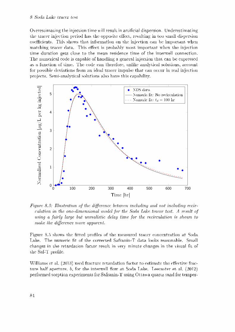
8 Soda Lake tracer test
Overestimating the injection time will result in arti�cial dispersion. Underestimatingthe tracer injection period has the opposite e�ect, resulting in too small dispersioncoe�cients. This shows that information on the injection can be important whenmatching tracer data. This e�ect is probably most important when the injectiontime duration gets close to the mean residence time of the interwell connection.The numerical code is capable of handling a general injection that can be expressedas a function of time. The code can therefore, unlike analytical solutions, accountfor possible deviations from an ideal tracer impulse that can occur in real injectionprojects. Semi-analytical solutions also have this capability.
0 100 200 300 400 500 600 7000
1
2
3
4
5
Time [hr]
Normalized
Concentration
[µg/Lper
kginjected]
NDS data
Numeric �t: No recirculation
Numeric �t: td = 100 hr
Figure 8.3: Illustration of the di�erence between including and not including recir-culation in the one-dimensional model for the Soda Lake tracer test. A result ofusing a fairly large but unrealistic delay time for the recirculation is shown tomake the di�erence more apparent.
Figure 8.5 shows the �tted pro�les of the measured tracer concentration at SodaLake. The numeric �t of the corrected Safranin-T data looks reasonable. Smallchanges in the retardation factor result in very minute changes in the visual �t ofthe Saf-T pro�le.
Williams et al. (2013) used fracture retardation factor to estimate the e�ective frac-ture half aperture, b, for the interwell �ow at Soda Lake. Leecaster et al. (2012)performed sorption experiments for Safranin-T using Ottawa quartz sand for temper-
84

8.2 Analysis of tracer data
0 100 200 300 400 500 600 7000
1
2
3
4
5
Time [hr]
Normalized
Concentration
[µg/Lper
kginjected]
NDS data
Numeric �t: td = 10 hr
No recirculation
Figure 8.4: Fitted 1,6-NDS tracer pro�le using a realistic 10 hour delay time alongwith the same model without the e�ects of recirculation.
atures up to 160◦C. Williams et al. (2013) used the results of the sorption experimentto estimate the surface-area-base partition coe�cient, Ka, for Safranin-T. Their cal-culations yielded Ka values ranging from 2.3 · 10−5 cm3/cm2 to 2.3 · 10−4 cm3/cm2.Williams et al. argue that using these values will overestimate the surface area tovolume ratio, b−1. For the volcanic tu� at Soda Lake a 35 times larger Ka value isprobably more appropriate (Williams et al., 2013). Using this and Rf = 3.49, with
Rf = 1 +Ka
b
results in a fracture half aperture of about 3-30 µm. Williams et al. believe such asmall fracture aperture to be too small to support the �ow rates at Soda Lake. Toosmall an estimate is due to the implicit assumption in the above equation, modellingthe �ssure walls as smooth surfaces when in fact they will be rough. A site speci�cassessment of the factor Ka should be performed to make these sort of calculationsmore reliable.
Williams et al. (2013) discuss alternative ways of estimating the �ow-path surfacearea at Soda Lake. Using a double-porosity model which does not allow the tracerto di�use further into the matrix than a certain skin depth, they estimated anupper-bound for the fracture half aperture to be about 1-0.1 mm. They also found
85
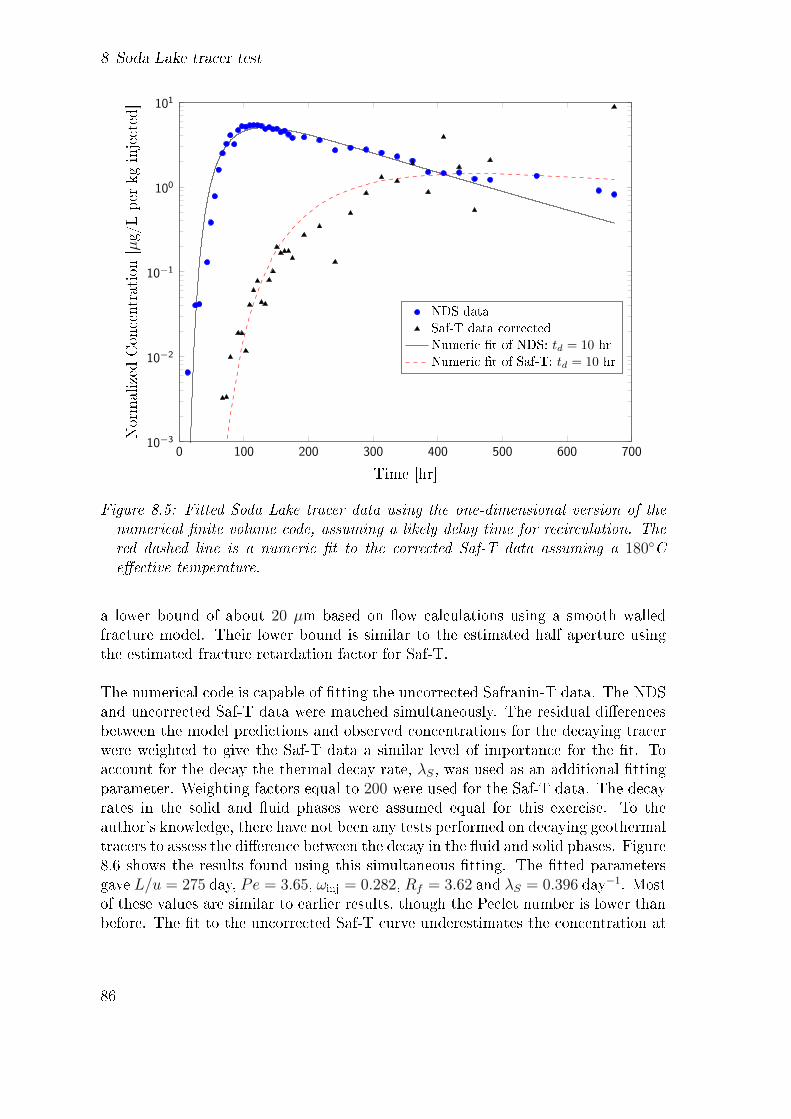
8 Soda Lake tracer test
0 100 200 300 400 500 600 70010−3
10−2
10−1
100
101
Time [hr]
Normalized
Concentration
[µg/Lper
kginjected]
NDS data
Saf-T data corrected
Numeric �t of NDS: td = 10 hr
Numeric �t of Saf-T: td = 10 hr
Figure 8.5: Fitted Soda Lake tracer data using the one-dimensional version of thenumerical �nite volume code, assuming a likely delay time for recirculation. Thered dashed line is a numeric �t to the corrected Saf-T data assuming a 180◦Ce�ective temperature.
a lower bound of about 20 µm based on �ow calculations using a smooth walledfracture model. Their lower bound is similar to the estimated half aperture usingthe estimated fracture retardation factor for Saf-T.
The numerical code is capable of �tting the uncorrected Safranin-T data. The NDSand uncorrected Saf-T data were matched simultaneously. The residual di�erencesbetween the model predictions and observed concentrations for the decaying tracerwere weighted to give the Saf-T data a similar level of importance for the �t. Toaccount for the decay the thermal decay rate, λS, was used as an additional �ttingparameter. Weighting factors equal to 200 were used for the Saf-T data. The decayrates in the solid and �uid phases were assumed equal for this exercise. To theauthor's knowledge, there have not been any tests performed on decaying geothermaltracers to assess the di�erence between the decay in the �uid and solid phases. Figure8.6 shows the results found using this simultaneous �tting. The �tted parametersgave L/u = 275 day, Pe = 3.65, ωinj = 0.282, Rf = 3.62 and λS = 0.396 day−1. Mostof these values are similar to earlier results, though the Peclet number is lower thanbefore. The �t to the uncorrected Saf-T curve underestimates the concentration at
86
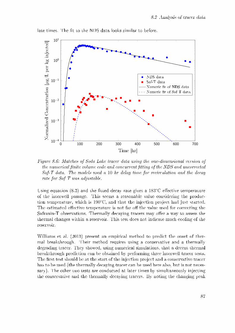
8.2 Analysis of tracer data
late times. The �t to the NDS data looks similar to before.
0 100 200 300 400 500 600 70010−4
10−3
10−2
10−1
100
101
Time [hr]
Normalized
Concentration
[µg/Lper
kginjected]
NDS data
Saf-T data
Numeric �t of NDS data
Numeric �t of Saf-T data
Figure 8.6: Matches of Soda Lake tracer data using the one-dimensional version ofthe numerical �nite volume code and concurrent �tting of the NDS and uncorrectedSaf-T data. The models used a 10 hr delay time for recirculation and the decayrate for Saf-T was adjustable.
Using equation (8.3) and the �tted decay rate gives a 183◦C e�ective temperatureof the interwell passage. This seems a reasonable value considering the produc-tion temperature, which is 190◦C, and that the injection project had just started.The estimated e�ective temperature is not far o� the value used for correcting theSafranin-T observations. Thermally decaying tracers may o�er a way to assess thethermal changes within a reservoir. This test does not indicate much cooling of thereservoir.
Williams et al. (2013) present an empirical method to predict the onset of ther-mal breakthrough. Their method requires using a conservative and a thermallydegrading tracer. They showed, using numerical simulations, that a decent thermalbreakthrough prediction can be obtained by performing three interwell tracer tests.The �rst test should be at the start of the injection project and a conservative tracerhas to be used (the thermally decaying tracer can be used here also, but is not neces-sary). The other two tests are conducted at later times by simultaneously injectingthe conservative and the thermally decaying tracers. By noting the changing peak
87

8 Soda Lake tracer test
concentrations of the decaying tracer, an empirical formula can be used to calculatethe thermal breakthrough time. For this method to be of use, enough time has topass between all the tests to allow for some cooling to take place along the �ow-path.If the time is not long enough then the di�erences in peak concentrations for thedecaying tracer will not be noticeable. The wait must not be too long, otherwisethe method is not of much use if breakthrough has already occurred.
8.2.2 Overestimation of fracture retardation
Looking back at Figures 8.4 and 8.5, it seems possible that the �tted pro�les shownresult in an overestimation of the fracture retardation factor. The �tting of the Saf-T data is essentially only taking the peak values of the Saf-T curve into account,due to the tracer's decay and delay, unlike the �tting of the NDS data, for which theearly and late concentrations are observed. The matched pro�le of the conservativetracer shows overestimation at some early times, underestimation at the peak andunderestimation at late times. This is not observed in the �tting of the decayingtracer. For the Saf-T �ts the peak observations are quite similar to the matchedpro�le. Therefore it appears that there is some inherent disparity when the pro�lesare �tted together to obtain the fracture retardation factor. This would probablybe less of a problem if the one-dimensional model �tted the pro�les better.
Here it is suggested that �tting of the early tracer breakthroughs may give an im-proved estimation of the fracture retardation. By �tting only the �rst twenty NDSobservations simultaneously with all the Saf-T data a retardation factor of 2.61 isfound. The twentieth NDS observation was measured about 120 hours after injec-tion. Technically, the �t of the Saf-T data should only account for data up to atime Rf times the 120 hours, but the retardation was not overly sensitive to thatadjustment. The �tted pro�les are shown in Figure 8.7. The �tted pro�les do afairly poor job of predicting late tracer concentrations but the early breakthroughsare predicted accurately. The matched pro�les are therefore at least consistent, un-like in the earlier analysis. Using this retardation factor and Ka = 8 · 10−3 cm3/cm2
gives a slightly more realistic calculated fracture half aperture of about 50 µm. Thisis only about a factor of 2-20 smaller than the upper-bound limits of the fractureaperture estimated by Williams et al. (2013). Using an upper-bound is probablyadvisable for thermal predictions, since it is best not to underestimate the coolingby overestimating the �ow-channel surface area.
88
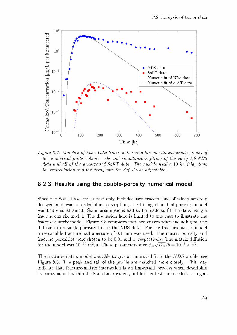
8.2 Analysis of tracer data
0 100 200 300 400 500 600 70010−4
10−3
10−2
10−1
100
101
Time [hr]
Normalized
Concentration
[µg/Lper
kginjected]
NDS data
Saf-T data
Numeric �t of NDS data
Numeric �t of Saf-T data
Figure 8.7: Matches of Soda Lake tracer data using the one-dimensional version ofthe numerical �nite volume code and simultaneous �tting of the early 1,6-NDSdata and all of the uncorrected Saf-T data. The models used a 10 hr delay timefor recirculation and the decay rate for Saf-T was adjustable.
8.2.3 Results using the double-porosity numerical model
Since the Soda Lake tracer test only included two tracers, one of which severelydecayed and was retarded due to sorption, the �tting of a dual-porosity modelwas badly constrained. Some assumptions had to be made to �t the data using afracture-matrix model. The discussion here is limited to one case to illustrate thefracture-matrix model. Figure 8.8 compares matched curves when including matrixdi�usion to a single-porosity �t for the NDS data. For the fracture-matrix modela reasonable fracture half aperture of 0.1 mm was used. The matrix porosity andfracture porosities were chosen to be 0.01 and 1, respectively. The matrix di�usionfor the model was 10−10 m2/s. These parameters give φm
√Dm/b = 10−3 s−1/2.
The fracture-matrix model was able to give an improved �t to the NDS pro�le, seeFigure 8.8. The peak and tail of the pro�le are matched more closely. This mayindicate that fracture-matrix interaction is an important process when describingtracer transport within the Soda Lake system, but further tests are needed. Using at
89

8 Soda Lake tracer test
least two di�erent conservative tracers, which have considerably di�erent moleculardi�usion coe�cients, may help to determine the extent of tracer di�usion.
0 100 200 300 400 500 600 7000
1
2
3
4
5
Time [hr]
Normalized
Concentration
[µg/Lper
kginjected]
NDS data
Numeric �t with matrix di�usion
Numeric �t without matrix di�usion
Figure 8.8: Comparison of matched pro�les using single- and double-porosity modelsto �t the 1,6-NDS tracer data using the numerical �nite volume code. The modelsused a 10 hr delay time.
90

9 Laugaland tracer tests
A series of three tracer tests were conducted over a two year period at Laugalandlow-temperature geothermal �eld, N-Iceland, see Figure 9.1. The tracer experimentswere concluded in the latter part of 1999. The tracer experiments and monitoringare described in detail in Axelsson et al. (2001), Axelsson et al. (2000a) and Axelssonet al. (2000b).
The natural recharge to the Laugaland geothermal system is very limited, which hasled to considerable pressure drawdown within the system, since production began in1977. The system's rock mass is mostly impermeable basalt and the �uid �ow of thesystem is con�ned to fractures. Reinjection of spent geothermal �uid was consideredas a possible way to limit pressure drawdown within the system and increase the longterm energy extraction from the system's 90-100◦C hot rock matrix. The tracer andmonitoring experiments had the objective of determining the feasibility and impactof reinjecting water back into the Laugaland �eld (Axelsson et al., 2001). Subject totheir tracer test interpretation, Axelsson et al. (2001) concluded that an average longterm reinjection rate of 15 L/s should be workable and could allow for an additionalenergy extraction of about 24 GWhth per year.
Figure 9.2 shows the relative locations of the injection and production wells withinthe Laugaland geothermal �eld. The production wells are believed to be connectedto one another through a near vertical SW-NE trending fracture zone (Axelssonet al., 2000b). Axelsson et al. estimated the direction of the fracture zone usingwell-logs. Their results are consistent with the inferred fracture zone from the low-resistivity structure stretching from the Laugaland to the Botn geothermal �eld, seeFigure 9.1.
91
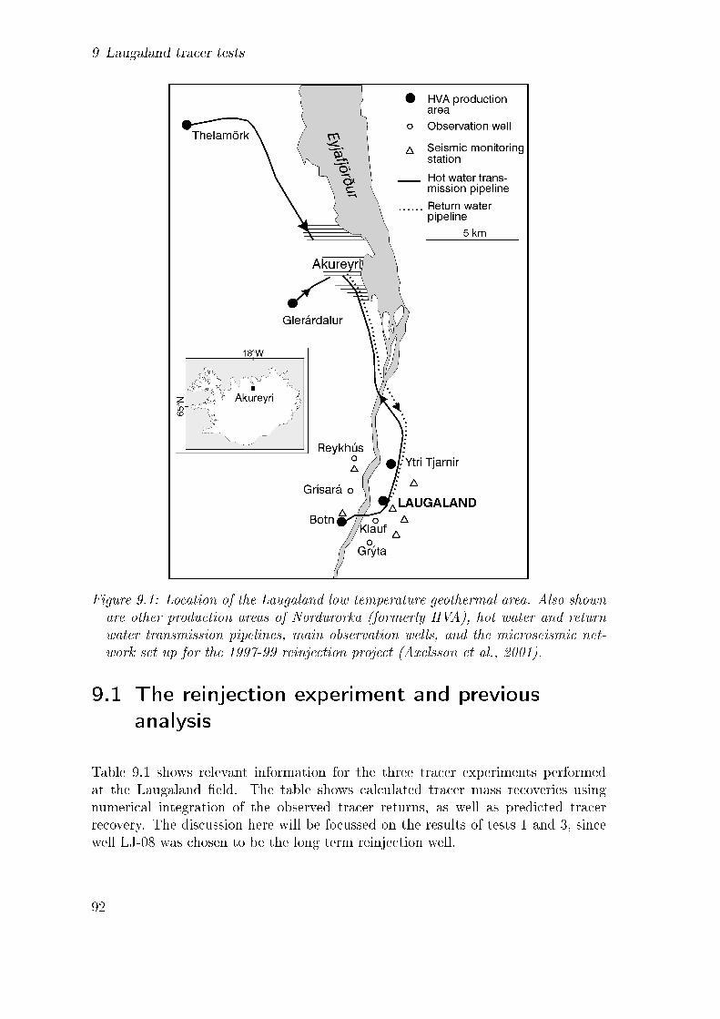
9 Laugaland tracer tests
Figure 9.1: Location of the Laugaland low-temperature geothermal area. Also shownare other production areas of Nordurorka (formerly HVA), hot water and returnwater transmission pipelines, main observation wells, and the microseismic net-work set up for the 1997-99 reinjection project (Axelsson et al., 2001).
9.1 The reinjection experiment and previous
analysis
Table 9.1 shows relevant information for the three tracer experiments performedat the Laugaland �eld. The table shows calculated tracer mass recoveries usingnumerical integration of the observed tracer returns, as well as predicted tracerrecovery. The discussion here will be focussed on the results of tests 1 and 3, sincewell LJ-08 was chosen to be the long term reinjection well.
92
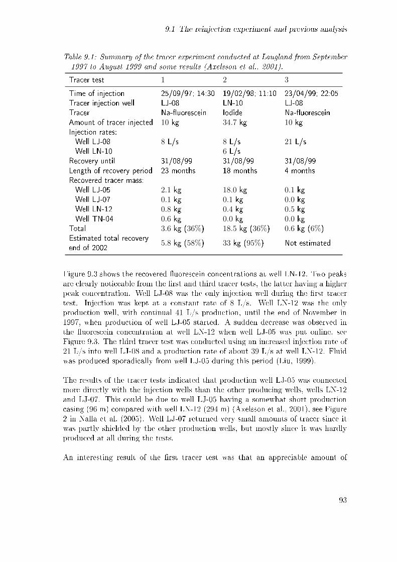
9.1 The reinjection experiment and previous analysis
Table 9.1: Summary of the tracer experiment conducted at Laugland from September1997 to August 1999 and some results (Axelsson et al., 2001).
Tracer test 1 2 3
Time of injection 25/09/97; 14:30 19/02/98; 11:10 23/04/99; 22:05Tracer injection well LJ-08 LN-10 LJ-08Tracer Na-�uorescein Iodide Na-�uoresceinAmount of tracer injected 10 kg 34.7 kg 10 kgInjection rates:Well LJ-08 8 L/s 8 L/s 21 L/sWell LN-10 6 L/s
Recovery until 31/08/99 31/08/99 31/08/99Length of recovery period 23 months 18 months 4 monthsRecovered tracer mass:Well LJ-05 2.1 kg 18.0 kg 0.1 kgWell LJ-07 0.1 kg 0.1 kg 0.0 kgWell LN-12 0.8 kg 0.4 kg 0.5 kgWell TN-04 0.6 kg 0.0 kg 0.0 kg
Total 3.6 kg (36%) 18.5 kg (36%) 0.6 kg (6%)Estimated total recovery
5.8 kg (58%) 33 kg (95%) Not estimatedend of 2002
Figure 9.3 shows the recovered �uorescein concentrations at well LN-12. Two peaksare clearly noticeable from the �rst and third tracer tests, the latter having a higherpeak concentration. Well LJ-08 was the only injection well during the �rst tracertest. Injection was kept at a constant rate of 8 L/s. Well LN-12 was the onlyproduction well, with continual 41 L/s production, until the end of November in1997, when production of well LJ-05 started. A sudden decrease was observed inthe �uorescein concentration at well LN-12 when well LJ-05 was put online, seeFigure 9.3. The third tracer test was conducted using an increased injection rate of21 L/s into well LJ-08 and a production rate of about 39 L/s at well LN-12. Fluidwas produced sporadically from well LJ-05 during this period (Liu, 1999).
The results of the tracer tests indicated that production well LJ-05 was connectedmore directly with the injection wells than the other producing wells, wells LN-12and LJ-07. This could be due to well LJ-05 having a somewhat short productioncasing (96 m) compared with well LN-12 (294 m) (Axelsson et al., 2001), see Figure2 in Nalla et al. (2005). Well LJ-07 returned very small amounts of tracer since itwas partly shielded by the other production wells, but mostly since it was hardlyproduced at all during the tests.
An interesting result of the �rst tracer test was that an appreciable amount of
93
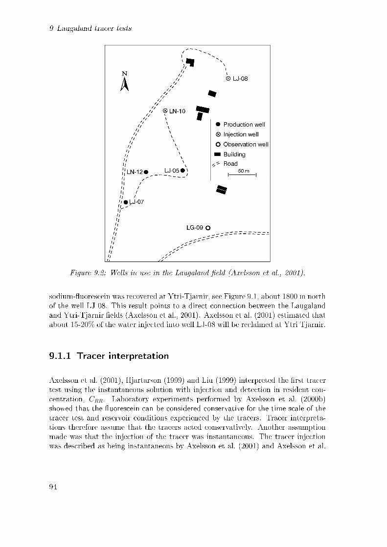
9 Laugaland tracer tests
Figure 9.2: Wells in use in the Laugaland �eld (Axelsson et al., 2001).
sodium-�uorescein was recovered at Ytri-Tjarnir, see Figure 9.1, about 1800 m northof the well LJ-08. This result points to a direct connection between the Laugalandand Ytri-Tjarnir �elds (Axelsson et al., 2001). Axelsson et al. (2001) estimated thatabout 15-20% of the water injected into well LJ-08 will be reclaimed at Ytri Tjarnir.
9.1.1 Tracer interpretation
Axelsson et al. (2001), Hjartarson (1999) and Liu (1999) interpreted the �rst tracertest using the instantaneous solution with injection and detection in resident con-centration, CRR. Laboratory experiments performed by Axelsson et al. (2000b)showed that the �uorescein can be considered conservative for the time scale of thetracer test and reservoir conditions experienced by the tracers. Tracer interpreta-tions therefore assume that the tracers acted conservatively. Another assumptionmade was that the injection of the tracer was instantaneous. The tracer injectionwas described as being instantaneous by Axelsson et al. (2001) and Axelsson et al.
94

9.1 The reinjection experiment and previous analysis
Oct97 Jan98 Apr98 Jul98 Nov98 Feb99 May99 Aug99 Nov990
2
4
6
8Fluorescein
[µg/L]
Figure 9.3: Measured �uorescein recovery in well LN-12.
(2000b). Recirculation of tracer mass was not an important factor during the tracertests. Less than 0.4 kg of �uorescein was reinjected back into the system over thetwo year test period (Axelsson et al., 2001). The rate of tracer reinjection is there-fore negligible compared with the initially injected amount. The measured tracerresponse in well LN-12 during the �rst tracer test was matched for the period beforewell LJ-05 went online.
Results of the tracer analysis performed by Axelsson et al. (2001), Hjartarson (1999)and Liu (1999) are compared in Table 9.2. Their simulations assumed three �ow-channels. The assumed channel lengths, L, are dissimilar between the foregoingauthors. Borehole logging indicated that about half of the �uid injected into wellLJ-08 exits into a shallow feedzone at a depth of about 320 m (Hjartarson, 1999).Liu speculated that the three simulated channels connected this shallow feedzone tothree feedzones at well LN-12 at depths of about 310 m, 670 m and below 1100 m.Hjartarson (1999) chose the channel lengths in a similar way. He considered that the�rst channel connects feedzones at depths of 325 m and 310 m, at wells LJ-08 andLN-12, respectively. Hjartarson chose the length of the second channel to re�ect aspeculated connection between a feedzone at a depth of 600 m at well LJ-08 and afeedzone at a 1140 m depth at well LN-12. His third channel is supposed to accountfor �ow between the two wells, through permeable interbeds. A tracer test usingstraddle packers to isolate feedzones within wells could be used, to determine whichfeedzones are in actual fact connected.
95

9 Laugaland tracer tests
Table 9.2: Previous results from interpreting the �rst tracer test at Laugaland.The tracer returns at well LN-12 were interpreted using the instantaneous, one-dimensional CRR solution and assuming three �ow-paths. The dispersion coe�-cients is assumed to be D = αu.
Channel L [m] u [m/day] φA [m2] α [m] m/M L/u [day] Pe
Axelssonet
al.(200
1)
1 300 63.0 0.098 61 0.0087 4.8 4.92 500 41.5 0.53 264 0.0304 12 1.93 1000 14.7 1.08 62 0.0229 68 16
Total 0.0620
Hjartarson
(199
9)
1 500 112 0.049 88 0.0077 4.5 5.72 800 69.1 0.30 366 0.029 12 2.23 350 5.18 3.7 26 0.027 68 13
Total 0.0637
Liu
(199
9)
1 312 60.4 0.186 63 0.016 5.2 5.02 405 23.4 0.588 89 0.020 17 4.63 1100 16.4 1.257 87 0.029 67 13
Total 0.065
Figure 9.4 shows the �tted curve found by (Axelsson et al., 2001). The �tted pro-�le gives a very close match to the observed concentrations. That pro�le can becompared with the one found by Liu, see Figure 9.5. Hjartarson's simulation isnot shown here, but his simulatios look similar to the ones of Axelsson et al.. Thedi�erent curves found by Axelsson et al. (2001), Hjartarson (1999) and Liu (1999)are in essence equally good matches to the data. This highlights the non-uniquenessof the solutions. Nevertheless, the obtained solutions have very similar features. Allof the simulations mentioned above show a very similar looking channel responsefor the third channel at late times. The channel lengths themselves do not decidethe shape of the matched curves, they simply scale the spatial coordinates, and asa result regulate the magnitude of the mean velocity and di�usivity. Comparingthe non-dimensional Peclet number of the di�erent channels and the mean residencetime, L/u, shows the similarity of the di�erent solutions. All three solutions predicta comparable total tracer return of about 6.4% from the �rst tracer test at well LN-12. They also predict a similar overall �ow-path volume. Assuming a 7% e�ective�ow-channel porosity, the sum of the �ow-path volumes is estimated to be about2 · 104 m3 (Axelsson et al., 2001). Nalla et al. (2005) interpreted the �rst Laugalandtracer test using a method of moments. Their results pointed to a 4.5 ·104 m3 sweptpore volume, twice the �ow-path volume estimate by Axelsson et al. (2001).
96
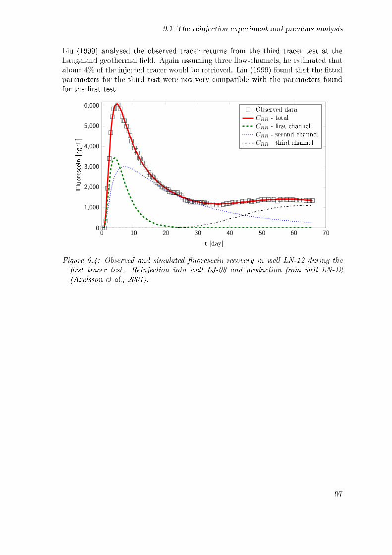
9.1 The reinjection experiment and previous analysis
Liu (1999) analysed the observed tracer returns from the third tracer test at theLaugaland geothermal �eld. Again assuming three �ow-channels, he estimated thatabout 4% of the injected tracer would be retrieved. Liu (1999) found that the �ttedparameters for the third test were not very compatible with the parameters foundfor the �rst test.
0 10 20 30 40 50 60 700
1,000
2,000
3,000
4,000
5,000
6,000
t [day]
Fluorescein[ng/L]
Observed data
CRR - total
CRR - �rst channel
CRR - second channel
CRR - third channel
Figure 9.4: Observed and simulated �uorescein recovery in well LN-12 during the�rst tracer test. Reinjection into well LJ-08 and production from well LN-12(Axelsson et al., 2001).
97

9 Laugaland tracer tests
0 10 20 30 40 50 60 700
1,000
2,000
3,000
4,000
5,000
6,000
t [day]
Fluorescein[ng/L]
Observed data
CRR - total
CRR - �rst channel
CRR - second channel
CRR - third channel
Figure 9.5: Measured and simulated �uorescein recovery in well LN-12 during the�rst tracer test (Liu, 1999).
9.2 Revised analysis of the Laugaland tracer tests
The Laugaland tracer tests, performed between injection well LJ-08 and productionwell LN-12, were re-examined using some of the models discussed in section 3.3. Forthe revised simulations, the injection was assumed to be instantaneous, in agreementwith the description of the tracer experiments.
9.2.1 The �rst tracer test
The �rst tracer test at Laugaland clearly indicated that wells LJ-08 and LN-12 areconnected by two distinct �ow-paths. The tracer returns show, see Figure 9.4, twode�nite peaks. The late arriving peak cannot be explained by recirculation, sincethe amount of recirculated tracer is not substantial enough. The �rst tracer testwas, accordingly, matched using two �ow-channels. The length of the two channelswere chosen to be consistent with those given by Axelsson et al. (2001).
Table 9.3 shows results of matching the tracer returns at well LN-12 during the �rstexperiment. The tracer concentrations were matched for the �rst 66 days of thetracer test. All four of the solutions types gave comparably close �ts to the data.The CFF solution gave the closest match. Figure 9.6 presents the best �ts foundfor the models having detection in �ux concentration. The �tted pro�les capture
98
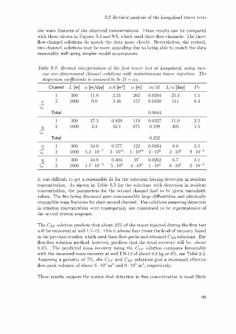
9.2 Revised analysis of the Laugaland tracer tests
the main features of the observed concentrations. These results can be comparedwith those shown in Figures 9.4 and 9.5, which used three �ow-channels. The three�ow-channel solutions do match the data more closely. Nevertheless, the revised,two channel, solutions may be more appealing due to being able to match the datareasonably well using simpler model assumptions.
Table 9.3: Revised interpretation of the �rst tracer test at Laugaland, using vari-ous one-dimensional (linear) solutions with instantaneous tracer injection. Thedispersion coe�cients is assumed to be D = αu.
Channel L [m] u [m/day] φA [m2] α [m] m/M L/u [day] Pe
CFF
1 300 11.8 2.31 263 0.0394 25.4 1.12 1000 9.0 3.46 157 0.0450 111 6.4
Total 0.0844
CRF
1 300 27.3 0.829 119 0.0327 11.0 2.52 1000 3.3 42.1 671 0.199 305 1.5
Total 0.232
CFR 1 300 34.0 0.577 122 0.0284 8.8 2.5
2 1000 5.2 · 10−7 3 · 1015 1 · 1010 2 · 106 2 · 109 9 · 10−8
CRR 1 300 44.8 0.404 97 0.0262 6.7 3.1
2 1000 1.7 · 10−3 5 · 108 4 · 106 1 · 103 6 · 105 2 · 10−4
It was di�cult to get a reasonable �t for the solutions having detection in residentconcentration. As shown in Table 9.3 for the solutions with detection in residentconcentration, the parameters for the second channel had to be given unrealisticvalues. The �ts being discussed gave unreasonably large di�usivities and physicallyimpossible mass fractions for their second channel. The solutions assuming detectionin resident concentration were consequently not considered to be representative ofthe actual system response.
The CRF solution predicts that about 23% of the tracer injected during the �rst testwill be recovered at well LN-12. This is almost four times the level of recovery foundin the previous studies, which used three �ow-paths and assumed CRR solutions. The�ux-�ux solution method, however, predicts that the total recovery will be. about8.4%. The predicted mass recovery using the CFF solution compares favourablywith the measured mass recovery at well LN-12 of about 0.8 kg or 8%, see Table 9.2.Assuming a porosity of 7%, the CFF and CRF solutions give a estimated e�ective�ow-path volumes of about 6 · 104 m3 and 6 · 105 m3, respectively.
These results support the notion that detection in �ux concentration is most likely
99
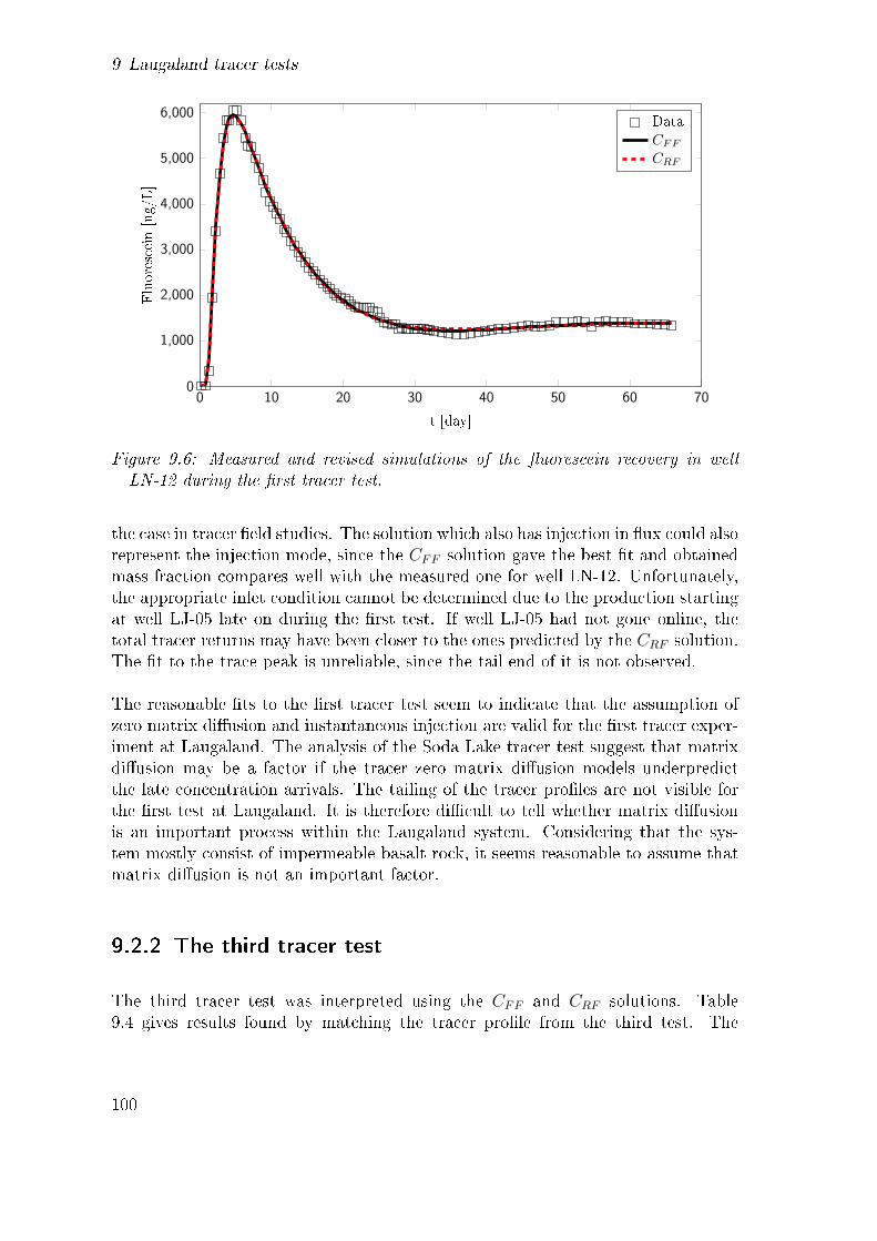
9 Laugaland tracer tests
0 10 20 30 40 50 60 700
1,000
2,000
3,000
4,000
5,000
6,000
t [day]
Fluorescein[ng/L]
Data
CFF
CRF
Figure 9.6: Measured and revised simulations of the �uorescein recovery in wellLN-12 during the �rst tracer test.
the case in tracer �eld studies. The solution which also has injection in �ux could alsorepresent the injection mode, since the CFF solution gave the best �t and obtainedmass fraction compares well with the measured one for well LN-12. Unfortunately,the appropriate inlet condition cannot be determined due to the production startingat well LJ-05 late on during the �rst test. If well LJ-05 had not gone online, thetotal tracer returns may have been closer to the ones predicted by the CRF solution.The �t to the trace peak is unreliable, since the tail end of it is not observed.
The reasonable �ts to the �rst tracer test seem to indicate that the assumption ofzero matrix di�usion and instantaneous injection are valid for the �rst tracer exper-iment at Laugaland. The analysis of the Soda Lake tracer test suggest that matrixdi�usion may be a factor if the tracer zero matrix di�usion models underpredictthe late concentration arrivals. The tailing of the tracer pro�les are not visible forthe �rst test at Laugaland. It is therefore di�cult to tell whether matrix di�usionis an important process within the Laugaland system. Considering that the sys-tem mostly consist of impermeable basalt rock, it seems reasonable to assume thatmatrix di�usion is not an important factor.
9.2.2 The third tracer test
The third tracer test was interpreted using the CFF and CRF solutions. Table9.4 gives results found by matching the tracer pro�le from the third test. The
100
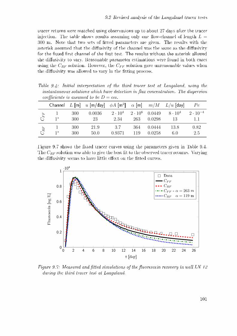
9.2 Revised analysis of the Laugaland tracer tests
tracer returns were matched using observations up to about 27 days after the tracerinjection. The table shows results assuming only one �ow-channel of length L =300 m. Note that two sets of �tted parameters are given. The results with theasterisk assumed that the di�usivity of the channel was the same as the di�usivityfor the �tted �rst channel of the �rst test. The results without the asterisk allowedthe di�usivity to vary. Reasonable parameter estimations were found in both casesusing the CRF solution. However, the CFF solution gave unreasonable values whenthe di�usivity was allowed to vary in the �tting process.
Table 9.4: Initial interpretation of the third tracer test at Laugaland, using theinstantaneous solutions which have detection in �ux concentration. The dispersioncoe�cients is assumed to be D = αu.
Channel L [m] u [m/day] φA [m2] α [m] m/M L/u [day] Pe
CFF 1 300 0.0036 2 · 104 2 · 106 0.0449 8 · 104 2 · 10−4
1∗ 300 23 2.34 263 0.0298 13 1.1
CRF 1 300 21.9 3.7 364 0.0444 13.8 0.82
1∗ 300 50.0 0.9371 119 0.0258 6.0 2.5
Figure 9.7 shows the �tted tracer curves using the parameters given in Table 9.4.The CRF solution was able to give the best �t to the observed tracer returns. Varyingthe di�usivity seems to have little e�ect on the �tted curves.
0 2 4 6 8 10 12 14 16 18 20 22 24 260
0.2
0.4
0.6
0.8
1·104
t [day]
Fluorescein[ng/L]
Data
CFF
CRF
CFF - α = 263 m
CRF - α = 119 m
Figure 9.7: Measured and �tted simulations of the �uorescein recovery in well LN-12during the third tracer test at Laugaland.
101
9 Laugaland tracer tests
Comparing the parameters in Table 9.4 with the values found for the �rst test, indi-cates some inconsistency between the two tests or that some incorrect assumptionswere made in the �tting process. This incompatibility is likely due to the �ow con-ditions being di�erent for each test. According to Liu (1999), the production ratefrom well LN-12 was less stable during the third test. The production rate variedbetween 38 L/s and 44 L/s during the third test. Moreover, well LJ-05 producedintermittently during the third test, unlike for the �tted period of the �rst test (Liu,1999). The assumption of the interwell �ow being at steady state is clearly notcorrect for the third test. Increasing the injection rate and well-head pressure at theinjection well will also change the �ow within the system. Considering these factsit is easy to see why the results of the two tests did not compare well.
Attempts were made to simultaneously �t the observed data from the �rst andthird tests. Some assumptions were made regarding the �ow-channels involved.The �tting procedure assumed the same two �ow-channels as given in Table 9.3.The simultaneous �tting was unable to give good matches. Part of the problemwas that the third test did not last long enough to show the second peak, whichwas visible in the �rst test. The �tting algorithm was therefore inclined to assumetwo peaks at early times. The most likely reason for the incompatibility of the twotests is that the �ow conditions were quite di�erent between the two experiments,as already mentioned.
9.3 Thermal predictions
Axelsson et al. (2001), Hjartarson (1999) and Liu (1999) used their tracer interpre-tations to forecast possible thermal breakthrough at well LN-12, due to reinjectionat well LJ-08. Hjartarson (1999) predicted that the production temperature atwell LN-12 would only decline by about 1◦C after 30 years of reinjection, assumingproduction of 41 L/s and injection of 8 L/s. Axelsson et al. (2001) made similarpredictions, but for a wider range of injection rates. Axelsson et al. (2001) predicteda 2◦C temperature decline after 30 years, for an average reinjection of 20 L/s anda 40 L/s production rate. Axelsson et al. (2001), Hjartarson (1999) and Liu (1999)used equation (4.8) for their thermal predictions with φf = 0.07.
Following the initial analysis of the tracer tests in 1999, well LJ-08 was chosen as thelong term injection well for the Laugaland site. The temperatures of the productionwells are monitored at Laugaland. Figure 9.8 shows the observed temperatures atwells LN-12, LJ-05 and LJ-07. The noise in the temperature data is mainly dueto short interruptions of production. Interestingly, wells LJ-07 and LJ-05 do notshow e�ects of thermal breakthrough, due to reinjection. According to Gautasonet al. (2012), the recent drop in the measured temperature at well LJ-05 is because of
102
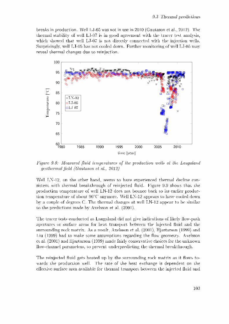
9.3 Thermal predictions
breaks in production. Well LJ-05 was not in use in 2010 (Gautason et al., 2012). Thethermal stability of well LJ-07 is in good agreement with the tracer test analysis,which showed that well LJ-07 is not directly connected with the injection wells.Surprisingly, well LJ-05 has not cooled down. Further monitoring of well LJ-05 mayreveal thermal changes due to reinjection.
1980 1985 1990 1995 2000 2005 201060
65
70
75
80
85
90
95
100
time [year]
Tem
perature
[◦C]
LN-12
LJ-05
LJ-07
Figure 9.8: Measured �uid temperatures of the production wells at the Laugalandgeothermal �eld (Gautason et al., 2012)
Well LN-12, on the other hand, seems to have experienced thermal decline con-sistent with thermal breakthrough of reinjected �uid. Figure 9.9 shows that theproduction temperature of well LN-12 does not bounce back to its earlier produc-tion temperature of about 96◦C anymore. Well LN-12 appears to have cooled downby a couple of degrees C. The thermal changes at well LN-12 appear to be similarto the predictions made by Axelsson et al. (2001).
The tracer tests conducted at Laugaland did not give indications of likely �ow-pathapertures or surface areas for heat transport between the injected �uid and thesurrounding rock matrix. As a result, Axelsson et al. (2001), Hjartarson (1999) andLiu (1999) had to make some assumptions regarding the �ow geometry. Axelssonet al. (2001) and Hjartarson (1999) made fairly conservative choices for the unknown�ow-channel parameters, to prevent underpredicting the thermal breakthrough.
The reinjected �uid gets heated up by the surrounding rock matrix as it �ows to-wards the production well. The rate of the heat exchange is dependent on thee�ective surface area available for thermal transport between the injected �uid and
103
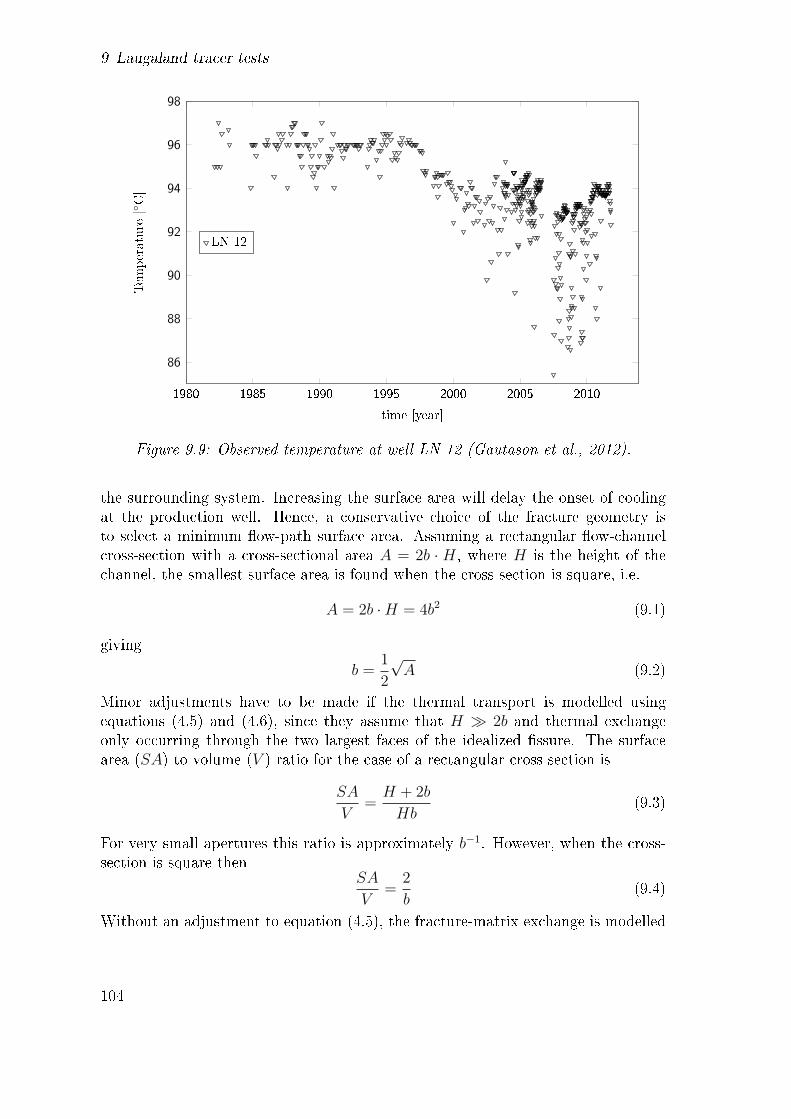
9 Laugaland tracer tests
1980 1985 1990 1995 2000 2005 2010
86
88
90
92
94
96
98
time [year]
Tem
perature
[◦C]
LN-12
Figure 9.9: Observed temperature at well LN-12 (Gautason et al., 2012).
the surrounding system. Increasing the surface area will delay the onset of coolingat the production well. Hence, a conservative choice of the fracture geometry isto select a minimum �ow-path surface area. Assuming a rectangular �ow-channelcross-section with a cross-sectional area A = 2b · H, where H is the height of thechannel, the smallest surface area is found when the cross-section is square, i.e.
A = 2b ·H = 4b2 (9.1)
giving
b =1
2
√A (9.2)
Minor adjustments have to be made if the thermal transport is modelled usingequations (4.5) and (4.6), since they assume that H � 2b and thermal exchangeonly occurring through the two largest faces of the idealized �ssure. The surfacearea (SA) to volume (V ) ratio for the case of a rectangular cross section is
SA
V=H + 2b
Hb(9.3)
For very small apertures this ratio is approximately b−1. However, when the cross-section is square then
SA
V=
2
b(9.4)
Without an adjustment to equation (4.5), the fracture-matrix exchange is modelled
104
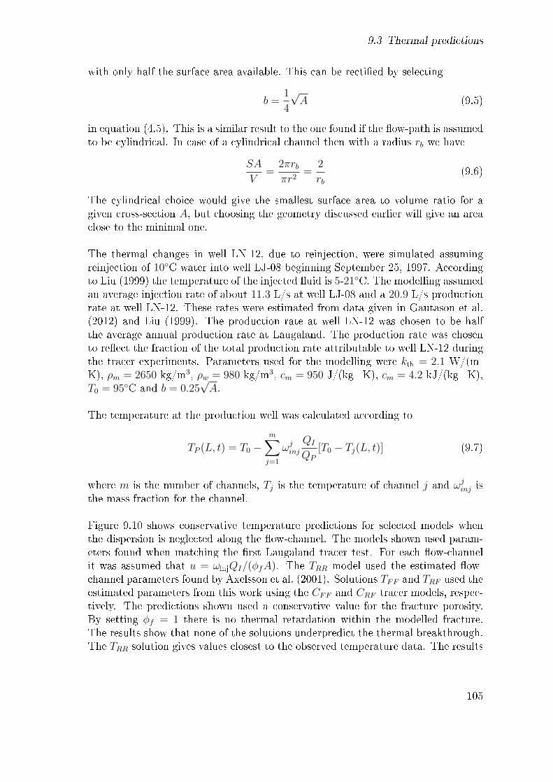
9.3 Thermal predictions
with only half the surface area available. This can be recti�ed by selecting
b =1
4
√A (9.5)
in equation (4.5). This is a similar result to the one found if the �ow-path is assumedto be cylindrical. In case of a cylindrical channel then with a radius rb we have
SA
V=
2πrbπr2
=2
rb(9.6)
The cylindrical choice would give the smallest surface area to volume ratio for agiven cross-section A, but choosing the geometry discussed earlier will give an areaclose to the minimal one.
The thermal changes in well LN-12, due to reinjection, were simulated assumingreinjection of 10◦C water into well LJ-08 beginning September 25, 1997. Accordingto Liu (1999) the temperature of the injected �uid is 5-21◦C. The modelling assumedan average injection rate of about 11.3 L/s at well LJ-08 and a 20.9 L/s productionrate at well LN-12. These rates were estimated from data given in Gautason et al.(2012) and Liu (1999). The production rate at well LN-12 was chosen to be halfthe average annual production rate at Laugaland. The production rate was chosento re�ect the fraction of the total production rate attributable to well LN-12 duringthe tracer experiments. Parameters used for the modelling were kth = 2.1 W/(mK), ρm = 2650 kg/m3, ρw = 980 kg/m3, cm = 950 J/(kg K), cm = 4.2 kJ/(kg K),T0 = 95◦C and b = 0.25
√A.
The temperature at the production well was calculated according to
TP (L, t) = T0 −m∑j=1
ωjinjQI
QP
[T0 − Tj(L, t)] (9.7)
where m is the number of channels, Tj is the temperature of channel j and ωjinj isthe mass fraction for the channel.
Figure 9.10 shows conservative temperature predictions for selected models whenthe dispersion is neglected along the �ow-channel. The models shown used param-eters found when matching the �rst Laugaland tracer test. For each �ow-channelit was assumed that u = ωinjQI/(φfA). The TRR model used the estimated �ow-channel parameters found by Axelsson et al. (2001). Solutions TFF and TRF used theestimated parameters from this work using the CFF and CRF tracer models, respec-tively. The predictions shown used a conservative value for the fracture porosity.By setting φf = 1 there is no thermal retardation within the modelled fracture.The results show that none of the solutions underpredict the thermal breakthrough.The TRR solution gives values closest to the observed temperature data. The results
105
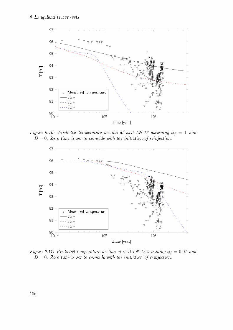
9 Laugaland tracer tests
10−1 100 10190
91
92
93
94
95
96
97
Time [year]
T[◦C]
Measured temperature
TRR
TFF
TRF
Figure 9.10: Predicted temperature decline at well LN-12 assuming φf = 1 andD = 0. Zero time is set to coincide with the initiation of reinjection.
10−1 100 10190
91
92
93
94
95
96
97
Time [year]
T[◦C]
Measured temperature
TRR
TFF
TRF
Figure 9.11: Predicted temperature decline at well LN-12 assuming φf = 0.07 andD = 0. Zero time is set to coincide with the initiation of reinjection.
106

9.3 Thermal predictions
indicate that the CRF solution does not represent the system response very well.The estimated mass fraction of the second CRF �ow-path is likely far too high.
Figure 9.11 shows results of changing the �ow-channel porosity to a probable ef-fective porosity φf = 4% (Axelsson et al., 2001). In this case all three modelsunderpredict the cooling at well LN-12 after the �rst year until about the eighthyear after reinjection started. The �ux-�ux solution appears to give the best resultsin this case. The TRR solution underpredicts the cooling for the entire period afterthe onset of cooling. The shift of the predicted thermal fronts are consistent withthe thermal retardation factor within the fracture being about 9 for φf = 0.07. Thisis clear when comparing Figures 9.10 and 9.11.
Neither of the above predictions have included the channel dispersion, which was animportant factor when matching the observed tracer histories. Figure 9.12 showsresults when the dispersion is included. The calculations pro�les were found usingthe numerical transport algorithm developed in this work. Thermal di�usion parallelto the �ow was also considered. The e�ect of parallel thermal di�usion is negligiblesince its e�ect is about four orders smaller than the retarded fracture dispersion term.Interestingly, both the �ux-�ux and res-res solutions give very similar predictionswhen the �ow-channel dispersion was included. The two methods start to deviatesigni�cantly after about 20 years of reinjection. Again, the TRF solution does notgive good results. The parameters estimated for the second channel, using the CRFsolution, were likely not very good estimates.
The results for the TRR and TFF solutions appear to give useful predictions whenthe �ow-path dispersion is included in the thermal transport model. Both solu-tions overpredict the cooling during the �rst year of reinjection but underpredictthe cooling over the subsequent two years. Improved simulations can be obtainedusing more accurate injection and production rates. Figure 9.13 shows results usingaverage annual �ow-rates given by Gautason et al. (2012) and estimated average an-nual �ow rates from the data presented by Liu (1999). The predictions shown usedparameter estimates found using the instantaneous �ux-�ux solution to interpret the�rst tracer test. The solution which has φf = 0.07 and includes channel dispersiongave a reasonable account of the temperature changes at well LN-12. From nowon it will be assumed that this model gives the best representation of the thermalcooling at well LN-12.
The simulations using variable �ow-rates assumed an average injection rate of 8 L/sat well LJ-08 for the �rst year of reinjection. Figure 9.14 shows the �ow rates usedin the simulations. The injection rate increases to about 15 L/s for the followingfour years, resulting in rapid cooling of the simulated temperatures. Decreasing theinjection rate allowed the calculated temperature at well LN-12 to rebound backup to almost 95◦C at one point. Choosing a more accurate initial �ow rate clearlyimproved the thermal predictions. The late time forecasts are also in good agree-
107

9 Laugaland tracer tests
10−1 100 10190
91
92
93
94
95
96
97
Time [year]
T[◦C]
Measured temperature
TRR
TFF
TRF
Figure 9.12: Predicted temperature decline at well LN-12 assuming φf = 0.07 andD = αu. Zero time is set to coincide with the initiation of reinjection.
10−1 100 10190
91
92
93
94
95
96
97
Time [year]
T[◦C]
Measured temperature
TFF : D = 0 , φf = 0.07
TFF : D = αu , φf = 0.07
TFF : D = αu , φf = 1
Figure 9.13: Predicted temperature changes at well LN-12 using variable annualinjection and production �ow rates. Zero time is set to coincide with the initiationof reinjection.
108
9.3 Thermal predictions
ment with the observed temperatures. The model chosen for thermal predictions issomewhat inaccurate at the end of the �rst injection year. A possible explanationis that well LN-12 was not in production during that period (Liu, 1999), resultingin a lowered observed temperature. Note that the abrupt changes in the modelledtemperatures are due to the discontinuous �ow rates used in the simulations.
0 2 4 6 8 10 12 14
10
15
20
25
30
Time [year]
Flowrate
[L/s]
Injection rate at well LJ-08
Production rate at well LN-12
Figure 9.14: Injection and production rates used for the simulated temperaturesshown in Figure 9.13.
Figure 9.15 shows a temperature forecast for well LN-12, assuming production andinjection rates similar to current levels. The results indicate that most of the cool-ing, from the direct paths connecting wells LJ-08 and LN-12, has probably alreadyoccurred. The predictions indicate that the temperature may decline by about 0.5◦Cover the next 30 years. It should be noted that these thermal predictions only ac-count for the most direct pathways connecting the two wells. Further analysis isneeded for appropriate long term thermal predictions. Axelsson et al. (2001) esti-mated that thermal cooling from less direct transport modes may take a few decadesto reach the production wells.
109

9 Laugaland tracer tests
5 10 15 20 25 30 35 40 45 5090
91
92
93
94
95
96
97
Time [year]
T[◦C]
Measured temperature
Predicted temperature
Figure 9.15: Predicted temperature decline at well LN-12 within the Laugalandgeothermal �eld, assuming an average 20 L/s production rate at well LN-12 and a10 L/s injection rate at well LJ-08. Zero time is set to coincide with the initiationof reinjection in 1997.
9.4 Possible improvements
The thermal predictions found using estimated parameters from the Laugalandtracer tests compared well with the measured temperature changes at well LN-12.The tracer transport solution assuming injection and detection in �ux concentrationwas the preferred method for interpreting the tracer data. Results using the �ux-�uxtracer �ts showed that good thermal predictions were possible even though simpleanalytical solutions were used to interpret the tracer returns. The thermal predic-tions are mostly dependent on the assumed �ow-channel surface area and porosity.Other factors are less of an issue. Reasonably good estimates can be easily found forthermal properties of the geothermal �uid and the rock matrix, such as the thermalconductivity of the matrix and the heat capacities of the �uid and the rock.
The thermal predictions shown here can be improved upon. Some rough assumptionswere made regarding the injection and production rates. Use of accurate �ow datacould result in better agreement with the observations. Further improvements maybe made by using more specialized types of tracers for the tracer interpretation.
The tracer tests indicated that matrix di�usion is likely not an in�uential process
110
9.4 Possible improvements
a�ecting tracer transport within the Laugaland reservoir. It would be interestingto see results of a tracer experiment at the Laugaland �eld using two conservativetracers, which have considerably di�erent molecular di�usion coe�cients, to con�rmthat matrix di�usion of solutes is not an important process within the system.Additionally, a sorptive tracer could be included in the experiment to interrogatethe �ow-path surface area. If the assumption that matrix di�usion is negligibleholds, then the e�ective inferred surface area from the sorptive tracer data shouldbe fairly reliable, since di�usion and retardation will, in that case, not interferewith the interpretation. In such a case, the matching of the tracer returns shouldbe a well-constrained problem. The researcher will have to have in mind that theestimated surface area includes the surface roughness of the rock.
Safranin-T could be used for this purpose, given that the appropriate laboratoryexperiments would be conducted to �nd its sorption kinetics when in contact withrock types found at Laugaland. Thermal degradation within the Laugaland systemwould likely be a lesser problem than for the Soda Lake test, due to Laugaland's lowertemperature. Note that equation (8.3) is valid for temperatures between 160◦C and190◦C. The thermal degradation rate of Saf-T should be determined for temperaturesexpected at Laugaland, if the tracer is to be used.
Simultaneous �tting of the tracer and thermal responses as suggested by Co (2012),could be used to resolve the di�cult task of estimating e�ective �ow-path porositiesand surface areas. However, some thermal cooling will have to have taken place atthe production well for this method to be of use. This approach is therefore notsuitable for predicting the onset of thermal changes due to reinjection. The methodcan be used to calibrate thermal transport for long term predictions. Thermal single-well injection-withdrawal tests may o�er a way to determine e�ective heat transfersurface areas within geothermal systems (Kocabas, 2005, Kocabas and Horne, 1990).The relationship between the surface area estimates of sorptive tracer tests and heattransfer surface areas may perhaps be found by comparing concurrent measurementsof thermal and tracer returns, when carrying out a single-well test. The estimatedrelationship could potentially be extended to results of interwell tests conducted atthe same site to decouple the e�ect of surface roughness on the transport of sorbingtracers. There is still the clear drawback of the single-well tests that they only giveinformation about the local area around the injection well. Nevertheless, such amethod could at least give some likely ranges for the expected heat transfer areaand as a result improve thermal predictions.
111

10 Conclusions
Previous research discussing methods for tracer test interpretation and thermalbreakthrough forecasting within geothermal systems were reviewed. Interwell tracertests were concluded to be the main tool for early characterization of well connec-tivity. Analysis of interwell tests may be supplemented with data obtained fromsingle-well tests, but an interwell test should be the primary way for determiningthe likely e�ects of reinjecting cold waste water into a given geothermal reservoir.
A numerical code capable of describing both tracer and thermal transport was out-lined and implemented using MATLAB. The results of using the code illustrate theapplicability of using numerical methods for evaluating tracer transport in the sub-surface. The numerical algorithm is able to account for linear sorption, tracer decayand recirculation. Appropriate boundary conditions are also easily implemented us-ing the given numerical method. The numerical code was able to replicate knownanalytical solutions with a decent amount of accuracy. The accuracy of the nu-merical simulations can be increased by using grid and time step re�nement. Thescope of problems which the numerical code can solve is quite wide. The numericalalgorithm can in principle be used to calculate more general tracer transport thanshown in this dissertation.
Numerical inversion algorithms were also developed and realized using MATLAB.The standard Levenberg-Marquardt algorithm and a secant version of the same algo-rithm proved to be useful for history matching of tracer data. The secant algorithmshowed great promise, since it was able to save computational time by requiringfewer calculations of the objective function, than the standard Levenberg-Marquardtalgorithm.
The numerical tracer transport algorithm was used in conjunction with the devel-oped optimization codes to match observed tracer returns of a conservative tracerand a reactive tracer at the Soda Lake geothermal �eld in Nevada, USA. The resultscompared favourably with the results found by previous researchers, indicating thatthe numerical algorithms were implemented correctly. Including recirculation of thetracer mass during the simulations was shown to improve the �t of the modelledtracer returns to the measured data at Soda Lake. The simulations were improved byusing a non-zero recirculation delay time. Improved matches of the non-conservativeSafranin-T data were found by allowing for an adjustable decay rate in the �tting
113

10 Conclusions
process. The analysis of the non-conservative, thermally decaying tracer returnsat the Soda Lake tracer test implied an e�ective �ow-path temperature of about183◦C and a 0.1 mm e�ective �ow-channel aperture. An improved �t to the tracerreturns was found by allowing for tracer di�usion into the rock matrix surroundingthe simulated �ow-channel. The results indicated that matrix di�usion of tracersmay be an important process at Soda Lake. Further tests are needed using othertypes of tracers to con�rm these results.
The methods developed in this work were also used to re-examine tracer tests car-ried out at the Laugaland low-temperature �eld in N-Iceland. Simple analyticalsolutions describing tracer transport along a single porosity �ow-channel were ca-pable of giving a good match to the observed tracer concentrations assuming two�ow-channels. This is an improvement upon previous studies which had to assumethree �ow-paths. Estimated �ow-channel parameters, found from matching tracerreturns, were assumed when simulating thermal cooling, between a selected injec-tion and production well pair at Laugaland. The simulated thermal predictionswere fairly successful at describing the observed thermal breakthrough at one of theproduction wells. Assuming �ow-channel dispersion and allowing for the variable�ow rates gave the best thermal predictions. The thermal predictions indicate thatthermal drawdown due to reinjection at well LN-12 in Laugaland, at current levelsof production and injection, will not result in signi�cant cooling of produced �uidsover the next couple of decades. These predictions only apply for the fast �ow-pathsconnecting wells LJ-08 and LN-12 at Laugland. More detailed modelling is neededto estimate cooling at the production wells due to the distribution of cold reinjection�uid throughout the Laugaland geothermal �eld.
The main conclusion is that tracer test interpretations can be applied to real geother-mal �eld data and give valuable insights, which can be applied to predict futurethermal changes due to reinjection.
114

Bibliography
Ames, M., Li, K., and Horne, R. N. (2013). The utility of threshold reactive tracersfor characterizing temperature distributions in geothermal reservoirs. In Proceed-ings, 38th Workshop on Geothermal Reservoir Engineering, Stanford University,Stanford, California.
Arason, T., Bjornsson, G., Axelsson, G., et al. (2003). The geothermal reservoirengineering software package ICEBOX, user's manual. Report for the UNU GTP,Iceland.
Axelsson, G. Role and management of geothermal reinjection. In Short Course onGeothermal Development and Geothermal Wells, address = organized by UNU-GTP and LaGeo, in Santa Tecla, El Salvador, March 11-17, year=2012.
Axelsson, G. (2008). The importance of geothermal reinjection. In Workshop forDecision Makers on Direct Heating Use of Geothermal Resources in Asia, Tianjin,China. UNU-GTP, TBLRREM and TBGMED, CD.
Axelsson, G. (2013). Tracer tests in geothermal resource management. In EuropeanPhysical Journal Web of Conferences, volume 50.
Axelsson, G., Bjornsson, G., Flovenz, O., Kristmannsdottir, H., and Sverrisdottir,G. (1995). Injection experiments in low-temperature geothermal areas in Iceland.In Proceedings of the World Geothermal Congress, pages 1991�1996.
Axelsson, G., Bjornsson, G., and Montalvo, F. (2005). Quantitative interpretation oftracer test data. In Proceedings of the World Geothermal Congress, pages 24�29.
Axelsson, G., Flovenz, O. G., Hauksdottir, S., Hjartarson, A., and Liu, J. (2001).Analysis of tracer test data, and injection-induced cooling, in the Laugalandgeothermal �eld, N-Iceland. Geothermics, 30(6):697�725.
Axelsson, G., Flovenz, O. G., Hjartarson, A., Hauksdottir, S., Sverrisdottir, G.,Arnason, F., Arnason, A., and Bodvarsson, R. (2000a). Thermal energy extractionby reinjection from the Laugaland geothermal system in N-Iceland. In Proceedingsof the World Geothermal Congress, pages 3027�3032.
Axelsson, G., Hjartarson, A., Hauksdottir, S., Flovenz, O. G., Sverrisdottir, G., Ar-nason, F., Finnsson, M., Arnason, A., and Bodvarsson, R. (2000b). Demonstration
115
BIBLIOGRAPHY
of improved energy extraction from a fractured geothermal reservoir. TechnicalReport for Thermie Project GE-0060/96, Orkustofnun, National Energy Author-ity of Iceland.
Ayling, B. F. and Rose, P. E. (2013). Geochemical tracers: Capabilities and potentialfor geothermal reservoir characterisation. In Proceedings of the 35th New ZealandGeothermal Workshop.
Bear, J. and Cheng, A. H.-D. (2010). Modeling groundwater �ow and contaminanttransport. Springer Dordrecht, Heidelberg, London, New York.
Becker, M. W., Remmen, K., Reimus, P. W., and Tso�ias, G. P. (2013). Investi-gating well connectivity using ionic tracers. In Proceedings, 38th Workshop onGeothermal Reservoir Engineering, Stanford University, Stanford, California.
Becker, M. W. and Shapiro, A. M. (2000). Tracer transport in fractured crystallinerock: Evidence of nondi�usive breakthrough tailing. Water Resources Research,36(7):1677�1686.
Becker, M. W. and Shapiro, A. M. (2003). Interpreting tracer breakthrough tail-ing from di�erent forced-gradient tracer experiment con�gurations in fracturedbedrock. Water Resources Research, 39(1):1024.
Bodin, J., Delay, F., and De Marsily, G. (2003). Solute transport in a single fracturewith negligible matrix permeability: 1. Fundamental mechanisms. HydrogeologyJournal, 11(4):418�433.
Bodvarsson, G. (1972). Thermal problems in the siting of reinjection wells. Geother-mics, 1(2):63�66.
Boving, T. B. and Grathwohl, P. (2001). Tracer di�usion coe�cients in sedimentaryrocks: correlation to porosity and hydraulic conductivity. Journal of ContaminantHydrology, 53(1):85�100.
Brenner, H. (1962). The di�usion model of longitudinal mixing in beds of �nitelength. Numerical values. Chemical Engineering Science, 17(4):229�243.
Bromley, C., Mongillo, M., and Rybach, L. (2006). Sustainable utilization strategiesand promotion of bene�cial environmental e�ects�having your cake and eating ittoo. In Proceedings of the 28th New Zealand Geothermal Workshop.
Broyden, C. G. (1965). A class of methods for solving nonlinear simultaneous equa-tions. Mathematics of computation, 19(92):577�593.
Bullivant, D. P. and O'Sullivan, M. J. (1985). Some simple models of tracer tests.In Proceedings of the 7th New Zealand Geothermal Workshop, pages 55�60.
116

BIBLIOGRAPHY
Carslaw, H. and Jaeger, J. (1959). Conduction of Heat in Solids. Clarendon Press,Oxford, 2nd edition.
Co, C. K. D. (2012). Characterization of geothermal feedzones and interwell con-nectivity. Master's thesis, Stanford University.
Co, C. K. D. and Horne, R. N. (2012). Coupled temperature and tracer dataanalysis using a uniform porous channel model. Geothermal Resources CouncilTransactions, 36.
Council, N. R. (1996). Rock fractures and �uid �ow: Contemporary understandingand applications. National Academies Press.
Croucher, A. and O'Sullivan, M. (1998). Numerical methods for contaminant trans-port in rivers and estuaries. Computers & �uids, 27(8):861�878.
Croucher, A. E., O'Sullivan, M. J., Kikuchi, T., and Yasuda, Y. (2004). Eulerian�lagrangian tracer simulation with tough2. Geothermics, 33(4):503�520.
Danckwerts, P. (1953). Continuous �ow systems: distribution of residence times.Chemical Engineering Science, 2(1):1�13.
Dean, C., Reimus, P., Leecaster, K., Oates, J., Newell, D., and Petty, S. (2013).Laboratory experiments to characterize cation-exchanging tracer behavior at New-berry Crater, OR. In Proceedings, 38th Workshop on Geothermal Reservoir En-gineering, Stanford University, Stanford, California.
Dean, C., Reimus, P., and Newell, D. (2012). Evaluation of a cation exchangingtracer to interrogate fracture surface area in EGS systems. In Proceedings ofthe 37th Workshop on Geothermal Reservoir Engineering, Stanford University,Stanford, California.
Finsterle, S. (2007). iTOUGH2 User's Guide. Earth Sciences Division, LawrenceBerkeley National Laboratory, University of California, Berkeley, California.
Fossum, M. and Horne, R. N. (1982). Interpretation of tracer return pro�les atWairakei geothermal �eld using fracture analysis. Geothermal Resources CouncilTransactions, 6.
Freeze, R. A. and Cherry, J. A. (1979). Groundwater. Prentice-Hall, EnglewoodCli�s, NJ.
Gautason, B., Egilson, T., and Tryggvason, H. (2012). Norðurorka 2010. Eftirlitmeð jarðhitasvæðum og orkubúskap veitunnar. Technical Report ÍSOR-2012/068,Iceland GeoSurvey (ÍSOR).
Gelhar, L. W., Welty, C., and Rehfeldt, K. R. (1992). A critical review of data on�eld-scale dispersion in aquifers. Water Resources Research, 28(7):1955�1974.
117
BIBLIOGRAPHY
Ghergut, I., Behrens, H., Maier, F., Karmakar, S., and Sauter, M. (2011). A noteabout �heat exchange areas� as a target parameter for SWIW tracer tests. InProceedings, 36th Workshop on Geothermal Reservoir Engineering, Stanford Uni-versity, Stanford, California.
Ghergut, I., Behrens, H., and Sauter, M. (2013). Single-well tracer push-pull testsensitivity to fracture aperture and spacing. In Proceedings, 38th Workshop onGeothermal Reservoir Engineering, Stanford University, Stanford, California.
Grathwohl, P. (1998a). Di�usion in natural porous media: Contaminant trans-port, sorption/desorption and dissolution kinetics. Kluwer Academic Publishers,Boston.
Grathwohl, P. (1998b). Slow contaminant release: The necessity for en-hanced/natural attenuation. IAHS Publication(International Association of Hy-drological Sciences), (250):265�271.
Gringarten, A., Witherspoon, P., and Ohnishi, Y. (1975). Theory of heat extractionfrom fractured hot dry rock. Journal of Geophysical Research, 80(8):1120�1124.
Hjartarson, A. (1999). Analysis of reservoir data collected during reinjection intothe Laugaland geothermal system in Eyjafjordur, N-Iceland. Master's thesis, Uni-versity of Iceland.
Horne, R., Breitenbach, K., and Fossum, M. (1982). Retention of chemical tracers ingeothermal reservoirs. Technical report, Stanford University, Stanford, California.
Horne, R. N. (1982). E�ects of water injection into fractured geothermal reservoirs:A summary of experience worldwide. Technical report, Geothermal Program,Interdisciplinary Research in Engineering and Earth Sciences, Stanford University,Stanford, California.
Horne, R. N. and Rodriguez, F. (1981). Dispersion in tracer �ow in fractured geother-mal systems. In Proceedings of the 7th Workshop on Geothermal Reservoir Engi-neering, pages 103�107, Stanford University, Stanford, California.
Horne, R. N. and Rodriguez, F. (1983). Dispersion in tracer �ow in fractured geother-mal systems. Geophysical Research Letters, 10(4):289�292.
Jensen, C. L. (1983). Matrix di�usion and its e�ect on the modeling of tracer returnsfrom the fractured geothermal reservoir at Wairakei, New Zealand. Master's thesis,Stanford University.
Jensen, C. L. and Horne, R. N. (1983). Matrix di�usion and its e�ect on the mod-eling of tracer returns from the fractured geothermal reservoir at Wairakei, NewZealand. In Proceedings, 9th Workshop on Geothermal Reservoir Engineering,Stanford University, Stanford, California.
118
BIBLIOGRAPHY
Juliusson, E. (2012). Characterization of fractured geothermal reservoirs based onproduction data. PhD thesis, Stanford University.
Juliusson, E. and Horne, R. N. (2012). Analytical model for thermal response in afracture due to a change in �ow rate. Geothermal Resources Council Transactions,36.
Juliusson, E. and Horne, R. N. (2013). Optimization of injection scheduling infractured geothermal reservoirs. Geothermics, 48:80�92.
Jung, Y. and Pruess, K. (2012). A closed-form analytical solution for thermal single-well injection-withdrawal tests. Water Resources Research, 48(3).
Kaya, E., Zarrouk, S. J., and O'Sullivan, M. J. (2011). Reinjection in geothermal�elds: A review of worldwide experience. Renewable and Sustainable EnergyReviews, 15(1):47�68.
Kim, J. G. and Finsterle, S. (2003). Application of automatic di�erentiation inTOUGH2. In Proceedings, TOUGH Symposium, Lawrence Berkeley National Lab-oratory, Berkeley, California, May 12-14.
Kocabas, I. (1989). Analysis of tracer and thermal transients during reinjection.PhD thesis, Stanford University.
Kocabas, I. (2005). Geothermal reservoir characterization via thermal injectionback�ow and interwell tracer testing. Geothermics, 34(1):27�46.
Kocabas, I. (2010). Designing thermal and tracer injection back�ow tests. In Pro-ceedings of the World Geothermal Congress, pages 25�29.
Kocabas, I. and Horne, R. (1987). Analysis of injection-back�ow tracer tests infractured geothermal reservoirs. Technical report, Stanford University, Stanford,California.
Kocabas, I. and Horne, R. (1990). A new method of forecasting the thermal break-through time during reinjection in geothermal reservoirs. In Proceedings, 15thWorkshop on Geothermal Reservoir Engineering, Stanford University, Stanford,California.
Kocabas, I. and Islam, M. (2000a). Concentration and temperature transients inheterogeneous porous media: Part I: Linear transport. Journal of PetroleumScience and Engineering, 26(1):211�220.
Kocabas, I. and Islam, M. (2000b). Concentration and temperature transients inheterogeneous porous media: Part II: Radial transport. Journal of PetroleumScience and Engineering, 26(1):221�233.
119
BIBLIOGRAPHY
Kreft, A. and Zuber, A. (1978). On the physical meaning of the dispersion equationand its solutions for di�erent initial and boundary conditions. Chemical Engi-neering Science, 33(11):1471�1480.
Leecaster, K., Ayling, B., Mo�tt, G., and Rose, P. (2012). Use of Safranin T as areactive tracer for geothermal reservoir characterization. In Proceedings of the 37thWorkshop on Geothermal Reservoir Engineering, Stanford University, Stanford,California.
Leibundgut, C., Maloszewski, P., and Külls, C. (2009). Tracers in hydrology. JohnWiley & Sons.
Levenberg, K. (1944). A method for the solution of certain problems in least squares.Quarterly of applied mathematics, 2:164�168.
Liu, J. (1999). Reinjection and tracer tests in the Laugaland geothermal �eld, N-Iceland. In: Georgsson, L. (Ed.), Geothermal Training in Iceland, 1999. UnitedNations University Geothermal Training Programme, Reykjavik, pages 141-164.
Madsen, K. and Nielsen, H. B. (2010). Introduction to optimization and data �t-ting. http://www2.imm.dtu.dk/pubdb/views/edoc_download.php/5938/pdf/
imm5938.pdf. Last accessed: 08-01-2014.
Magnusdottir, L. and Horne, R. (2013). Fracture connectivity of fractal fracturenetworks estimated using electrical resistivity. In Proceedings, 38th Workshop onGeothermal Reservoir Engineering, Stanford University, Stanford, California.
Maier, F. and Kocabas, I. (2013a). Comment on �A closed-form analytical solutionfor thermal single-well injection-withdrawal tests� by Jung and Pruess. WaterResources Research, 49(1):640�643.
Maier, F. and Kocabas, I. (2013b). E�cient analytical solution for parameter es-timation of push shut-in pull experiments in an idealized single fracture system.In Proceedings, 38th Workshop on Geothermal Reservoir Engineering, StanfordUniversity, Stanford, California.
Malate, R. and O'Sullivan, M. (1991). Modelling of chemical and thermal changes inwell PN-26 Palinpinon geothermal �eld, Philippines. Geothermics, 20(5):291�318.
Maloszewski, P., Herrmann, A., and Zuber, A. (1999). Interpretation of tracer testsperformed in fractured rock of the Lange Bramke basin, Germany. HydrogeologyJournal, 7(2):209�218.
Maloszewski, P. and Zuber, A. (1990). Mathematical modeling of tracer behavior inshort-term experiments in �ssured rocks. Water Resources Research, 26(7):1517�1528.
120
BIBLIOGRAPHY
Maloszewski, P. and Zuber, A. (1997). Comment on �Convergent radial dispersion ina double-porosity aquifer with fracture skin: Analytical solution and applicationto a �eld experiment in fractured chalk� by Allen F. Moench. Water ResourcesResearch, 33(3):497�500.
Mannington, W., O'Sullivan, M., Bullivant, D., and Clotworthy, A. (2004). Rein-jection at Wairakei�Tauhara: A modelling case study. In Proceedings of the 29thWorkshop on Geothermal Reservoir Engineering, pages 166�173, Stanford Uni-versity, Stanford, California.
Marquardt, D. (1963). An algorithm for least squares estimation of nonlinear param-eters. Journal of the Society for Industrial and Applied Mathematics, 11:431�441.
Maturgo, O. O., Sanchez, D. R., and Barroca, G. B. (2010). Tracer test using naph-thalene disulfonates in Southern Negros Geothermal Production Field, Philip-pines. In Proceedings of the World Geothermal Congress.
Moench, A. F. (1989). Convergent radial dispersion: A Laplace transform solutionfor aquifer tracer testing. Water Resources Research, 25(3):439�447.
Moench, A. F. (1995). Convergent radial dispersion in a double-porosity aquiferwith fracture skin: Analytical solution and application to a �eld experiment infractured chalk. Water Resources Research, 31(8):1823�1835.
Nakamura, H. (1981). Development and utilization of geothermal energy in Japan.Geothermal Resources Council Transactions, 5.
Nalla, G., Shook, G. M., and Axelsson, G. (2005). Tracer test analysis for char-acterization of Laugaland geothermal �eld. In Proceedings, 30th Workshop onGeothermal Reservoir Engineering, Stanford University, Stanford, California.
Neretnieks, I. (1980). Di�usion in the rock matrix: An important factor in radionu-clide retardation? Journal of Geophysical Research, 85(B8):4379�4397.
Neretnieks, I., Eriksen, T., and Tähtinen, P. (1982). Tracer movement in a single�ssure in granitic rock: Some experimental results and their interpretation. WaterResources Research, 18(4):849�858.
Nield, D. A. and Bejan, A. (2006). Convection in porous media. Springer.
Novakowski, K., Bickerton, G., and Lapcevic, P. (2004). Interpretation of injection�withdrawal tracer experiments conducted between two wells in a large single frac-ture. Journal of Contaminant Hydrology, 73(1):227�247.
Novakowski, K. S. (1992). An evaluation of boundary conditions for one-dimensionalsolute transport: 2. Column experiments. Water Resources Research, 28(9):2411�2423.
121

BIBLIOGRAPHY
O'Sullivan, M. J., Pruess, K., and Lippmann, M. J. (2001). State of the art ofgeothermal reservoir simulation. Geothermics, 30(4):395�429.
Parker, J. (1984). Analysis of solute transport in column tracer studies. Soil ScienceSociety of America Journal, 48(4):719�724.
Parker, J. and Van Genuchten, M. T. (1984). Flux-averaged and volume-averagedconcentrations in continuum approaches to solute transport. Water ResourcesResearch, 20(7):866�872.
Parlange, J.-Y., Starr, J., Van Genuchten, M. T., Barry, D., and Parker, J. (1992).Exit condition for miscible displacement experiments. Soil Science, 153(3):165�171.
Patankar, S. V. (1980). Numerical heat transfer and �uid �ow. Taylor & Francis.
Peaceman, D. W. (1977). Fundamentals of numerical reservoir simulation. Elsevier.
Peters, G. P. and Smith, D. W. (2001). Numerical study of boundary conditions forsolute transport through a porous medium. International journal for numericaland analytical methods in geomechanics, 25(7):629�650.
Plasencia, M., Pedersen, A., Arnaldsson, A., and Jonsson, H. (2012). Geothermalmodel calibration using global minimization algorithm by mapping out objec-tive function minima and saddle points. In Proceedings, TOUGH Symposium,Lawrence Berkeley National Laboratory, Berkeley, California, September 17-19.
Press, W. H., Teukolsky, S. A., Vetterling, W. T., and Flannery, B. P. (1992).Numerical Recipes in C: The art of scienti�c computing 2nd Edition. CambridgeUniversity Press.
Pruess, K. (2002). Numerical simulation of multiphase tracer transport in fracturedgeothermal reservoirs. Geothermics, 31(4):475�499.
Pruess, K. and Doughty, C. (2010). Thermal single-well injection-withdrawal tracertests for determining fracture-matrix heat transfer area. In Proceedings, 35thWorkshop on Geothermal Reservoir Engineering, Stanford University, Stanford,California.
Pruess, K., O'Sullivan, M., and Kennedy, B. (2000). Modeling of phase-partitioningtracers in fractured reservoirs. In Proceedings, 25th Workshop on GeothermalReservoir Engineering, pages 24�26, Stanford University, Stanford, California.
Pruess, K., van Heel, T., and Shan, C. (2005). Tracer testing for estimating heattransfer area in fractured reservoirs. In Proceedings of the World GeothermalCongress.
122

BIBLIOGRAPHY
Reimus, P., Williams, M., Vermeul, V., Rose, P., Leecaster, K., Ayling, B., Sanjuan,R., Ames, M., Dean, C., and Benoit, D. (2012). Use of tracers to interrogate frac-ture surface area in single-well tracer tests in EGS systems. In Proceedings, 37thWorkshop on Geothermal Reservoir Engineering, Stanford University, Stanford,California.
Reimus, P. W. and Haga, M. J. (1999). Analysis of tracer responses in the BUL-LION forced-gradient experiment at Pahute Mesa, Nevada. Technical report, LosAlamos National Laboratory, Los Alamos, NM (US).
Rose, P., Benoit, W., Lee, S. G., Tandia, B., Kilbourn, P., and Station, W. P. (2000).Testing the naphthalene sulfonates as geothermal tracers at Dixie Valley, Ohaaki,and Awibengkok. In Proceedings, 25th Workshop on Geothermal Reservoir Engi-neering, Stanford University, Stanford, California.
Rose, P., Riasetto, D., Siy, J., Bartl, M., Reimus, P., Mella, M., Leecaster, K., andPetty, S. (2011). Quantum dots as tracers in geothermal and EGS reservoirs.In Proceedings, 36th Workshop on Geothermal Reservoir Engineering, StanfordUniversity, Stanford, California.
Rose, P. E., Benoit, W. R., and Kilbourn, P. M. (2001). The application of the pol-yaromatic sulfonates as tracers in geothermal reservoirs. Geothermics, 30(6):617�640.
Rose, P. E., Leecaster, K., Clausen, S., Sanjuan, R., Ames, M., Reimus, P., Williams,M., Vermeul, V., and Benoit, D. (2012). A tracer test at the Soda Lake, Nevadageothermal �eld using a sorbing tracer. In Proceedings, 37th Workshop on Geother-mal Reservoir Engineering, Stanford University, Stanford, California.
Rose, P. E., Mella, M., Kasteler, C., and Johnson, S. D. (2004). The estimationof reservoir pore volume from tracer data. In Proceedings, 29th Workshop onGeothermal Reservoir Engineering, Stanford University, Stanford, California.
Roubinet, D., Dreuzy, J.-R., and Tartakovsky, D. M. (2012). Semi-analytical so-lutions for solute transport and exchange in fractured porous media. Water Re-sources Research, 48(1).
Schwartz, R., McInnes, K., Juo, A., Wilding, L., and Reddell, D. (1999). Bound-ary e�ects on solute transport in �nite soil columns. Water Resources Research,35(3):671�681.
Shook, G. M. (2001). Predicting thermal breakthrough in heterogeneous media fromtracer tests. Geothermics, 30(6):573�589.
Shook, G. M. and Forsmann, J. H. (2005). Tracer interpretation using temporalmoments on a spreadsheet. Idaho National Laboratory.
123
BIBLIOGRAPHY
Stefansson, V. (1997). Geothermal reinjection experience. Geothermics, 26(1):99�139.
Sullivan, E. J., Reimus, P. W., and Counce, D. A. (2003). Transport of a reactivetracer in saturated alluvium described using a three-component cation-exchangemodel. Journal of Contaminant Hydrology, 62:675�694.
Transtrum, M. K. and Sethna, J. P. (2012). Improvements to the Levenberg-Marquardt algorithm for nonlinear least-squares minimization. ArXiv preprintarXiv:1201.5885.
Trew, M., O'Sullivan, M., Harvey, C., Anderson, E., and Pruess, K. (2000). Com-puter modelling of gas and liquid tracers in geothermal reservoirs. In Proceedings25th Workshop on Geothermal Reservoir Engineering, Stanford University, Stan-ford, California.
Van Genuchten, M. T. (1981). Analytical solutions for chemical transport withsimultaneous adsorption, zero-order production and �rst-order decay. Journal ofHydrology, 49(3):213�233.
Van Genuchten, M. T. (1985). Convective-dispersive transport of solutes involved insequential �rst-order decay reactions. Computers & Geosciences, 11(2):129�147.
Van Genuchten, M. T. and Parker, J. (1984). Boundary conditions for displace-ment experiments through short laboratory soil columns. Soil Science Society ofAmerica Journal, 48(4):703�708.
Van Genuchten, M. T. and Wagenet, R. (1989). Two-site/two-region models forpesticide transport and degradation: Theoretical development and analytical so-lutions. Soil Science Society of America Journal, 53(5):1303�1310.
Williams, M. D., Reimus, P., Vermeul, V. R., Rose, P., Dean, C. A., Watson, T. B.,Newell, D., Leecaster, K., and Brauser, E. (2013). Development of models to sim-ulate tracer tests for characterization of enhanced geothermal systems. Technicalreport, Paci�c Northwest National Laboratory (PNNL), Richland, WA (US).
Williams, M. D., Vermeul, V. R., Reimus, P., Newell, D., and Watson, T. (2010).Development of models to simulate tracer behavior in enhanced geothermal sys-tems: Status report. Technical report, Paci�c Northwest National Laboratory(PNNL), Richland, WA (US).
Wu, X., Pope, G. A., Shook, G. M., and Srinivasan, S. (2008). Prediction of en-thalpy production from fractured geothermal reservoirs using partitioning tracers.International Journal of Heat and Mass Transfer, 51(5):1453�1466.
Zuber, A. Models for tracer �ow. In Tracer Methods in Isotope Hydrology, A technicaldocument issued by the International Atomic Energy Agency, Vienna.
124