Prediction of extreme price occurrences in theGerman day-ahead electricity market

Lars Ivar Hagforsa, Hilde Hørthe Kamperudb, Florentina Paraschivc, MarcelProkopczukd, Alma Satorb and Sjur Westgaardb

April 2016

a Corresponding author. E-mail: lars.i.hagfors@iot.ntnu.no. Department of Industrial Economics and Technol-ogy Management, Norwegian University of Science and Technology, Alfred Getz vei 3, 7041 Trondheim, Norway.b Department of Industrial Economics and Technology Management, Norwegian University of Science andTechnology, Alfred Getz vei 3, 7041 Trondheim, Norway.c Institute for Operations Research and Computational Finance, University of St. Gallen, Bodanstr. 6, CH-9000,Switzerlandd School of Economics and Management, Leibniz University Hannover, Koenigsworther Platz 1, 30167 Han-nover, Germany

Marcel Prokopczuk and Sjur Westgaard gratefully acknowledge financial support from E.ON Stipendienfonds.

Abstract

Understanding the mechanisms that drive extreme negative and positive prices in day-ahead electricity pricesis crucial for managing risk and market design. In this paper, we consider the problem of understanding howfundamental drivers impact the probability of extreme price occurrences in the German day-ahead electricitymarket. We develop models using fundamental variables to predict the probability of extreme prices. The dy-namics of negative prices and positive price spikes differ greatly. Positive spikes are related to high demand,low supply, and high prices the previous days, and mainly occur during the morning and afternoon peak hours.Negative prices occur mainly during the night, and are closely related to low demand combined with high windproduction levels. Furthermore, we do a closer analysis of how renewable energy sources, hereby photovoltaicand wind power, impact the probability of negative prices and positive spikes. The models confirm that ex-tremely high and negative prices have different drivers, and that wind power is particularly important in rela-tion to negative price occurrences. The models capture the main drivers of both positive and negative extremeprice occurrences, and perform well with respect to accurately forecasting the probability with high levels ofconfidence. Our results suggests that probability models are well suited to aid in risk management for marketparticipants in day-ahead electricity markets.

Keywords: Energy Markets; Fundamental Analysis; Spikes; EPEX

i

1 Introduction

Electricity spot prices exhibit seasonality, mean-reversion, time-varying and at times high volatility, as well asoccasional price jumps. The spot price is determined by the intersection between the demand and the supplycurves, and the price for each period is set by the most expensive generator required to satisfy demand. Electric-ity markets have highly inelastic short term demand and a nonlinear convex supply curve. Consequently, therelationship between fundamentals and prices is complex and nonlinear. Electricity itself is a unique commod-ity since it is produced and consumed simultaneously, and offers no possibilities of storage of any significantcapacity. Available reserves are therefore always limited, and in times of scarcity and high demand the produc-ers with available capacity have market power. These producers can set asking prices well above marginal costscontributing to the extremely high prices occasionally observed in electricity markets (Bunn et al. (2016)). Thefollowing unique characteristics occasionally result in extreme prices; the prices may be very low and negativewhen supply exceeds demand, or extremely high when supply cannot fulfill the inelastic demand.

At each point in time there is a certain amount of supplying generators at different price levels available,thus making up the merit order curve. Until recently, the merit order curve has consisted of base load fromnuclear and coal first, up until the most expensive peak-load units, e.g., gas and oil. However, recently the shareof renewable energy sources has increased in many markets. Due to low marginal costs, renewable productionplaces before traditional large-scale base load plants when actively producing. For market participants suchas producers, retailers, risk managers and regulators it is vital being able to model the tails of the prices, tounderstand and adapt to the price related risk. Much of the risk related to trading in power markets is due tothe extreme tail price occurrences, either extremely low or high prices. Therefore, predicting and understandingthe tail behaviour of electricity prices is often more important than forecasting the expected price of a givenperiod. The German electricity market has seen a large increase of renewable energy sources, while at the sametime also having an increasing frequency of negative price occurrences and positive spikes. This makes the tailbehaviour of the German market particularly interesting to analyze.

The intermittent nature of renewable energy sources is challenging from a risk-management perspective, anincreasingly relevant issue in recent years. Lower than expected production from renewable sources may causedeficits and correspondingly high prices, which is a large source of risk for retailers. On the contrary, excessivelyhigh production may cause oversupply and low, or even negative, prices. When the spot price is negative,producers essentially pay for dumping electricity on the market. Opportunity cost of shutting/ramping downmay exceed the negative price of produced electricity; for example, there has been instances where utilitieswere willing to pay up to €120/MWh or more to get rid of the excess electricity produced (Keles et al., 2011).

Our paper identifies main drivers behind the occurrence of extreme prices at the German day-ahead elec-tricity market (European Power Exchange, EPEX), as well as predicting these occurrences. Literature on predic-tion of extreme electricity price behaviour is lacking, particularly for markets with a large share of intermittentrenewable energy and negative price occurrences. This suggests that tail behaviour of electricity spot pricesand causes of extreme price movements is currently not well understood. The first contribution of this paper isestimating logit models for forecasting the probability of an extreme price as a function of selected fundamentalvariables. This analysis reveals which fundamental variables drive the probability of extreme price occurrences,and quantifies the impact on the probability of observing extreme prices. Our study is the first, to our knowl-edge, which provides such a detailed overview of the link between fundamental variables which impact theprobability of spike occurrences. This marks a clear contribution to the literature stream on fundamental mod-eling and comes with complementary insights to existing VaR papers by Byström (2005) and Paraschiv et al.(2016). Currently, it is assumed that high levels of wind production is the main driver behind negative prices.Positive spikes are likely to be closely related to the relationship between demand and supply, in which renew-able energy sources are playing an increasingly important role. The second contribution of this paper is there-fore a further exploration of how forecasts of photovoltaic and wind power production affect the probability ofextreme prices.

1

2 Literature Review

Our paper can be placed in the context of two main research areas in the field of electricity spot price markets:(i) modeling of spike occurrences and behaviour, and (ii) the impact of renewable energy sources on electricityprices. There is an extensive amount of research on modeling and forecasting electricity spot prices. Yet, the lit-erature seems to be at the beginning of understanding the economic drivers behind extreme price occurrences– particularly in markets with a large share of renewable energy sources.

Different modelling techniques have been applied in order to capture and model the distribution of extremeprice behaviour. Bunn and Karakatsani (2003) gives an overview of several methods used for forecasting elec-tricity prices. Bunn et al. (2016) use a multifactor, dynamic, quantile regression formulation and show how theprice elasticities of the fundamentals vary extensively across quantiles. However, the elastisities of gas, coal andcarbon prices exhibit no specific pattern across quantiles hence they hardly have any influence on the peakprice distribution. Thomas et al. (2011) develop an autoregressive (AR) model to capture the effects of indi-vidual spikes while controlling for seasonality in spot price returns in the Australian electricity market. Theyconclude that incorporation of supply and demand information is necessary to adequately capture negativeprices. Christensen et al. (2012) extend the research on AR models by looking at the prediction of spikes usingan autoregressive conditional hazard (ACH) model on the Australian electricity market. As a benchmark, thelogit model is used, yielding similar results. Focusing on the short-term forecasts of spike occurrences, Eichleret al. (2013) develop variations of the dynamic binary response model, e.g. with regime-switching mechanisms,proposed by Kauppi and Saikkonen (2008). The models have a superior fit on the Australian market data andthey suggest to replace the logistic function by an asymmetric link function leading to significant improve-ments. Eichler et al. (2013) also extend the ACH model used in Christensen et al. (2012) by incorporating pastprice information with that improving the performance of the model. Karakatsani and Bunn (2010) apply vari-ous statistical models to investigate the relationship between fundamental drivers and electricity price volatilityin the UK market, which is a different piece of the puzzle for understanding extreme price behaviour.

In the litterature, the focus has shifted from forecasting prices based on the entire price distribution to iso-lating normal range prices from the price spikes. Byström (2005) and Paraschiv et al. (2016) investigate theperformance of EVT on accurately modeling and forecasting the extreme tails of electricity price distributions.Both studies conclude that EVT is a powerful tool for this purpose. Lu et al. (2005), Zhao et al. (2007b) and Zhaoet al. (2007a) model normal and extreme prices separately to achieve more complete and robust models andmore accurate forecasts. Zhao et al. (2007b) use a method based on data mining by applying two algorithmsto the data - support vector machine and probability classifier - to predict the spike occurrence. The resultsare highly accurate and provide improved risk management practices related to extreme price prediction, butprovide limited economic insights. Higgs and Worthington (2008) study the Australian spot electricity market,which exhibits frequent price spikes, and employ three models to capture these effects; a stochastic, a mean-reverting and a regime-switching part. The regime-switching model outperforms the other two because theallowance of price spikes is better. A shortcoming of the model is the unrealistic assumption of constant tran-sition probabilities. Mount et al. (2006) solves this issue by adjusting the regime-switching model by modelingthe transition probabilities as a function of the load and/or the implicit reserve margin. By modeling the volatilebehaviour of the electricity prices in the Pennsylvania-New Jersey-Maryland (PJM) Power Pool, they provide ac-curate spike predictions. However, the model is dependent on precise reserve margin measurements, whichare not easily obtained.

Regime switching models are frequently used to model spike behaviour (Arvesen et al. (2013), Huisman andde Jong (2003), Keles et al. (2011), Weron et al. (2004),Weron (2009), Weron and Misiorek (2005)). They allow thespot price to switch between a base regime and higher/lower jump regimes. Paraschiv et al. (2015) propose aregime-switching approach to simulate price paths and forecasts on the EPEX. They extend the approach fromKovacevic and Paraschiv (2014) to include serial dependencies and transition probability for spike clustering.Christensen et al. (2009) perform a Poisson AR framework to identify spikes defined as threshold exceedances.Keles et al. (2011) consider positive price spikes and negative prices at the EPEX by implementing a regime-switching model. All of the above-mentioned models focus mainly on positive spikes in markets dominated

2

by conventional energy sources. Consequently, the models are not including the impact of renewable energyproduction. Literature including the impact of renewable energy sources on spikes and negative prices is lim-ited. This particularly applies to negative prices, which have become increasingly more common in latter years(Paraschiv et al. (2014), Schneider and Schneider (2010) and Keles et al. (2011)).

Huisman et al. (2013) investigate the effect of renewable energy sources on electricity prices indirectly bystudying hydro power in the Nord Pool market. They argue that theoretical and simulation studies show declin-ing electricity prices when introducing sustainable energy supply, but empirical studies supporting this resultare scarce. Paraschiv et al. (2014) investigate directly the influence of renewable energy sources on the Germanelectricity market. By analyzing the impact of wind and photovoltaic on day-ahead spot prices at the EPEX, theyconclude that the introduction of renewable energy sources increase the extreme price behaviour and influencethe fuel mix for electricity production. Hagfors et al. (2016) expand the literature on renewable energy to theGerman market by looking at the effect of renewable power sources on EPEX price formation using quantile re-gression. They analyze the effect of wind and photovoltaic, and confirm the results from Paraschiv et al. (2014)that renewable energies have a dampening effect on the spot prices. Further they find that negative prices,mostly due to wind power, mainly occur during night hours when demand is low.

Our paper extends the research regarding how renewable energy sources impact the extreme electricityprice behaviour, in particular on the EPEX. In doing so, we complement the research by Paraschiv et al. (2014)by focussing on extreme price movements.

3 The German Electricity Market

The German electricity spot market has gone through large regulatory changes and energy input mix changes,as shown in Table 1. The regulatory changes have contributed to incentivizing an increased share of renewableenergy sources and contributed to a large expansion of renewable production. As the successor to the ElectricityFeed Act ("Stromeinspeisungsgesetz", StrEG) from 1991, the EEG was issued in 2000 and guarantees producersof renewable energy a minimum compensation price per kWh. The compensation is secured through feed-intariffs that come on top of the spot market prices. The EEG has stimulated a strong increase of installed pro-duction of renewable sources, changing the energy input mix vastly to include 14,6% renewable energy (8,9%wind, 5,7% photovoltaic) in 2014 (Table 1). The target of the EEG is to have 35% renewable production in 2035;consequently, renewable energy will likely continue to be incentivized, although the feed-in-tariffs have beenlowered in later years (Paraschiv et al. (2014)). Frondel et al. (2010) and Fanone et al. (2013) argue that increaseof renewable energy sources has reduced the average spot electricity prices, and even led to a number of occur-rences of negative prices. However, consumers have not experienced lower prices; the feed-in-tariffs exceed theprice reduction from increased renewable capacity. Further, Frondel et al. (2010) claim that government policyhas failed in introducing renewable energy in a cost-effective and viable way. On 1st of January 2010 the last sig-nificant regulatory change took place, the Equalization Mechanism Ordinance (AusglMechV). The AusglMechVobliges the Transmission System Operators (TSOs) to market the EEG-electricity on the day-ahead market, thusentirely changing the market mechanisms of trading energy from renewable sources.

The exchange based trading in the day-ahead market in Germany is conducted at the EPEX. Trading fordelivery on the next day opens at 12:00, and the exchange is active all year. The market is divided in 24 hourlyintervals, where a trading period is defined as a one hour period, e.g. 12:00-13:00. Market participants bid agiven quantity MWh in a trading period at a set price, where offered price must be in the range -€500/MWh to€3000/MWh. Negative prices have been allowed at the EPEX since 1st September 2008 to ensure market clearingin situations where supply exceeds demand (Genoese et al. (2010)).

3

Table 1: Percentagewise contribution of various fuel sources and production technologies out of the total energyproduction, making out the German energy input mix from 2009 to 2014, Energiebilanzen (2015).

2009 2010 2011 2012 2013 2014

Coal 42.6% 41.5% 42.8% 44.0% 45.2% 43.2%Nuclear 22.6% 22.2% 17.6% 15.8% 15.4% 15.8%Natural Gas 13.6% 14.1% 14.0% 12.1% 10.5% 9.5%Oil 1.7% 1.4% 1.2% 1.2% 1.0% 1.0%Wind 6.5% 6.0% 8.0% 8.1% 8.4% 8.9%Hydro power 3.2% 3.3% 2.9% 3.5% 3.2% 3.3%Biomass 4.4% 4.7% 5.3% 6.3% 6.7% 7.0%Photovoltaic 1.1% 1.8% 3.2% 4.2% 4.7% 5.7%Waste-to-energy 0.7% 0.7% 0.8% 0.8% 0.8% 1.0%Other 3.6% 4.2% 4.2% 4.1% 4.0% 4.3%

4 Data Analysis

4.1 Choice of Data and Descriptive Statistics

We analyze hourly PHELIX spot prices in the German electricity market observed between 4th of January 2010and 31st of May 2014, and model each hourly time series separately. At the beginning of 2010, large changes inthe energy input mix were coupled with the last significant regulatory change (AusglMechV). The properties ofelectricity prices differ considerably from those of financial assets. Electricity prices are seasonal, and exhibithigh volatility that might result in extremely high (or low) prices. Unlike most stock and commodity prices, spotelectricity prices are stationary. An augmented Dickey Fuller (ADF) test with two lags on the spot prices in oursample yields a statistic of -45.04, confirming the electricity price series are stationary.1

The descriptive statistics of spot prices are given in Table 3. The spot price ranges from negative €222/MWhto positive €210/MWh. However, the standard deviation of €16.6/MWh shows that large share of prices arerelatively close to the mean. The excess kurtosis is high, indicating a possibility of extreme prices in eitherdirection. The skewness is low and negative, implying prices below mean are more likely than prices abovemean.

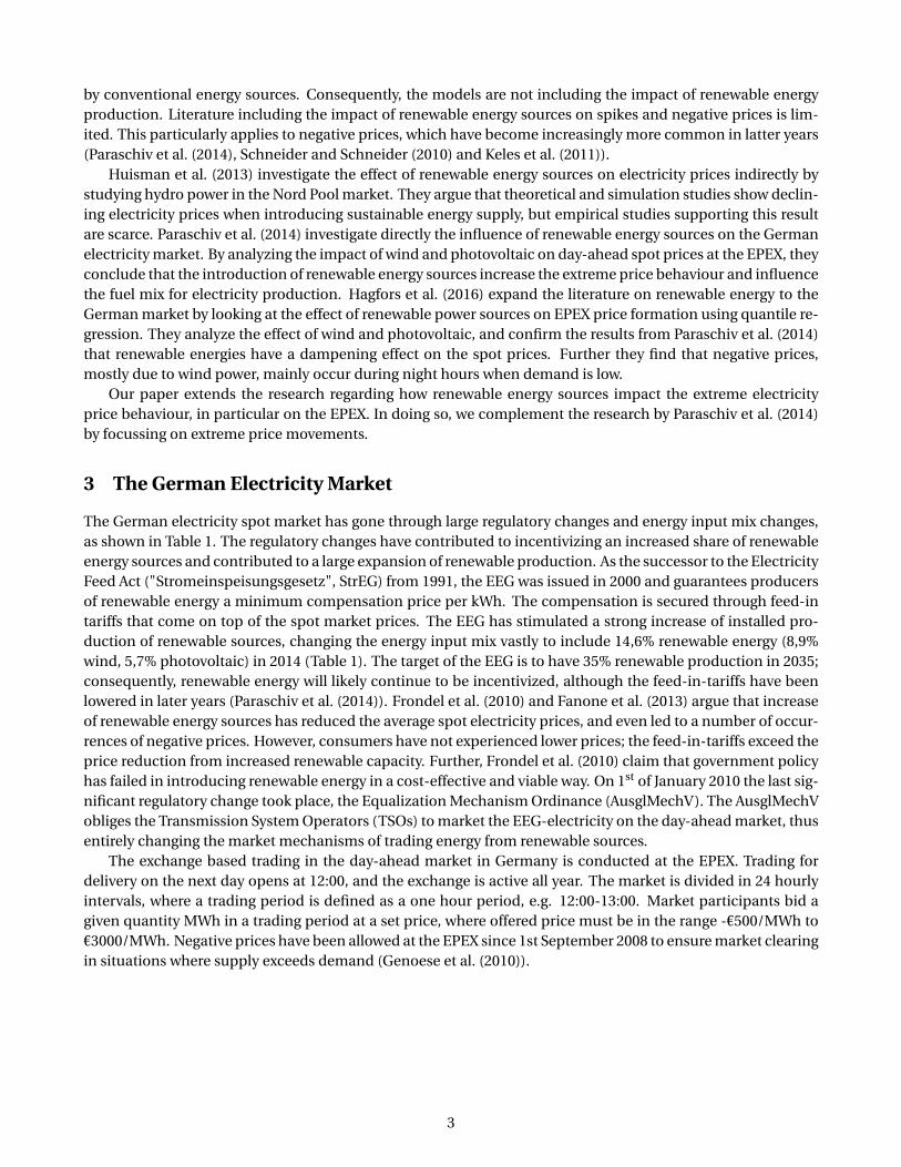
Electricity spot prices are complex to model, and can be linearly or non-linearly related to many variables.Table 2 shows the fundamental variables considered to explain the dynamics of electricity spot prices, as thesevariables are expected to impact the price formation. Lagged price 1 (day before) and 7 (a week before) havebeen included because of the high correlation between spot prices and lagged prices. Electricity demand ex-hibits predictable weekly patterns, and this is handled through the inclusion of seven-day lagged price. A teststatistic of 138 from a Ljung-Box test conducted with seven lags, confirms auto-correlation is present. To modelthe volatility, spot prices were first regressed on the seven first lags, and the regression residuals were used inan EWMA model with smoothing constant λ = 0.94. This method captures the seasonal effects, weekly trendsand auto-correlation between the first seven lags, and is a pragmatic representation of the volatility at eachpoint. Demand forecasts are not consistently published by the four TSOs in Germany, and thus need to bemodeled. Forecast data used in our analysis has been modeled according to the method described in Paraschivet al. (2014), thus seasonality is here handled. The analysis and modeling focuses on the effect of different sup-ply sources, and the modeling therefore separately considers power plant availability, wind, and photovoltaic.Each trading period has unique price dynamics, and demand/supply has been modelled accordingly.

Descriptive statistics of fundamental variables are provided in Table 3. It is worth noting that the wind fore-casts and photovoltaic forecasts have higher standard deviation than the other fundamental variables, as well

1All variables have been tested and found to be stationary with an ADF test, except for CO2 price and coal price. Intuitively they bothhave an upper and lower bound, and there is reason to expect that a longer time series of these prices would be found to be stationary.

4

Table 2: Overview of the variables chosen for modeling.

Variable, units Description Data source Granularity

Lag spot priceMarket clearing price for the same hour of the lastrelevant delivery day – lag 1 and 7

European Energy Exchange (EPEX) Hourly

Expected demand, MWhDemand forecast for the relevant hour on thedelivery day as modelled in Paraschiv et al. (2014)

Own data, German Weather Service Hourly

Expected wind power infeed, MWhExpected infeed published by German transmission systemoperators following the electricity price auction

Transmission system operatorshttp://www.50hertz.com/de/http://amprion.de/https://www.transnetbw.com/enhttp://www.tennet.eu/nl/home.html

Hourly

Expected photovoltaic infeed, MWhExpected infeed published by German transmission systemoperators following the electricity price auction

Transmission system operatorshttp://www.50hertz.com/de/http://amprion.de/https://www.transnetbw.com/enhttp://www.tennet.eu/nl/home.html

Hourly

Expected power plant availability, MWhEx ante expected power plant availability forelectricity production (voluntary publication)on the delivery day, published daily at 10:00 am

European EnergyExchange and transmissionsystem operators:ftp://infoproducts.eex.com

Hourly

Coal price, EUR/12,000 tLatest available price (daily auctioned) of the front-monthAmsterdam-Rotterdam-Antwerp (ARA)futures contract before the electricity auction takes place

European Energy Exchange Daily

Gas price, EUR/MWhLast price of the NCG Day Ahead Natural Gas Spot Price on the daybefore the electricity price auction takes place

Bloomberg, Ticker: GTHDAHD Index Daily

Oil price, EUR/bblLast price of the active ICE BrentCrudefutures contracton the day before theelectricity price auction takes place

Bloomberg, Ticker: COA Comdty Daily

Price for EUA, EUR 0.01/EUA 1000 t CO2Latest available price of the EPEXCarbon Index (Carbix), daily auctioned at 10:30 am

European Energy Exchange (EPEX) Daily

Spot price volatility Volatility at each data point based on an EWMA model European Energy Exchange(EPEX) Hourly

Table 3: Descriptive statistics of variables used for modeling. Lag 1/lag 7 have similar characteristics as spotprice, volatility is not included.

Spot price Demand Wind PV PPA Coal Gas Oil CO2

Mean 42.9 54852 5297 2514 55146 71.2 23.2 74.2 9.3Standard deviation 16.6 10081 4432 4280 4894 11.6 4.1 4.8 4.3Min -222.0 29201 229 0 40016 51.5 11.2 61.0 2.5Max 210.0 79884 26256 24525 64169 99.0 39.5 83.8 16.8Skewness -1.02 -0.05 1.52 2.04 -0.27 0.24 -0.63 -0.72 0.28Excess kurtosis 16.44 -1.04 2.30 3.75 -0.77 -1.08 0.88 -0.35 -1.48

as positive excess kurtosis and positive skew. These characteristics indicate there is a higher chance of very highforecasts of wind/photovoltaic production, and higher variability than, e.g. demand and power plant availabil-ity. Demand forecasts have negative excess kurtosis, indicating there is a low probability for very extreme valuesin either direction.

The scatter plot of wind forecasts versus spot prices shown in Figure 1 confirms that extremely low spotprices are seen nearly exclusively when wind production is high, in accordance with the negative correlation.This indicates that high forecasts of wind are a driver behind negative prices. The demand versus spot pricesconfirm that very high prices occur when demand is high, and that low prices occur when demand is low, inaccordance with the positive correlation. Very low prices are observed when demand forecasts are low, andwind forecasts are high – implying negative prices are due to either low demand, excess supply from wind, or acombination of factors.

5

(a) PHELIX spot price plotted against demand forecast. (b) PHELIX spot price plotted against wind forecast.

Figure 1: Scatter plots for demand forecast (a) and wind forecast (b) against the PHELIX spot price. The plotsshow that negative prices usually occur in combination with high wind production and low demand.

4.2 Definition of Extreme Prices and Analysis of Occurrences

Filtering extreme observations from normal is a challenging task that can be solved in various ways. Advancedexamples include using Markov regime switching models (Janczura and Weron (2010), Weron (2009)), waveletfiltering (Stevenson et al. (2006)), and thresholds implied by Gaussian prediction intervals (Borovkova and Per-mana (2006)). Simpler methods include setting a subjectively chosen fixed threshold (Eichler et al. (2013)), usea variable price threshold determined by a certain percentage of the highest prices classified as extreme (Trücket al. (2007)), classifying prices as spikes if they exceed the mean price by three standard deviations (Carteaand Figueroa (2005)) or determining the threshold using a joint maximum likelihood approach (Paraschiv et al.(2015)).

To estimate a logit model for extreme price prediction it is required to determine which price is consideredto be extreme. A reasonable approach is to filter out some percentage of the highest prices, typically 1%. Thismethod is simple to implement, but sufficiently powerful to be used for modeling, and yields a positive spikethreshold at €79.2/MWh. The drawback is that the threshold will vary as the data sample changes. Another op-tion is defining a fixed threshold based on a subjective perception of what classifies as extreme for market par-ticipants, e.g., €80/MWh, €90/MWh. Zhao et al. (2007a) argue the threshold can be set as the mean of the priceseries plus a multiple of the historically based volatility. Although the choice of threshold may seem arbitrary,1% of the highest prices is considered to be in the extreme end of the price distribution. We show in Section 5.4,that estimating the logit model using different thresholds yields similar results. The exact choice of thresholddoes therefore not impact the modelling performance excessively, as long as there are sufficiently many occur-rences to estimate the model while isolating extreme prices from the normal range. Negative extreme pricesare defined as prices below zero, with the assumption that these occurrences are considered extreme and havebeen highly unusual in electricity spot price markets until recent years. These definitions of extreme pricesyield 387 positive spikes and 177 negative prices – 1.00% and 0.46% of total observations.Base case is defined asprices in the normal range, meaning above zero and below €79.2.

Our analysis focuses on tail behaviour in electricity prices, where each probability model is based on a singletrading period. An overview of spike occurrences in Figure 2 clearly shows that most positive spikes occurwhen demand is high, between 17:00 – 19:00. Although demand is high during midday, there are far fewerpositive spikes; this might be due to the significantly higher solar production during those trading periods.Negative prices exhibit a slightly less predictable behaviour, and are observed in most of the trading periodswith the exception of the afternoon peak demand period. Negative prices are clearly most common during thenight, and occur when wind production is high and demand low compared to average values of each tradingperiod (Tables 14 and 13).Negative prices occurring during midday are, on average, much closer to zero thanobservations during night, implying that prices during the night are more likely to be extreme. Negative day-time prices seem to occur while the photovoltaic production forecast is very high, thus leading to oversupplyin the system. It is also noteworthy that demand forecast is lower than the overall mean of 54 852 MW for

6

Table 4: Overview of extreme price occurrences year 2010-14 (values for 2014 are linearly extrapolated based ondata from first 5 months).

2010 2011 2012 2013 2014

Positive spikes 91 65 131 93 17Negative spikes 12 15 56 64 72

entire sample when negative prices occur in daytime. Compared with Table 14, demand is also lower than themean of each trading period when negative prices occur, indicating the supply side is not adjusting accordingto demand, and prices can become extremely low.

Figure 2: Extreme price occurrences and average demand forecast and PV forecast per trading period.

The spikes are to some extent seasonally distributed, and occur primarily in winter. This might be related toelectricity prices in winter being higher in general, combined with higher demand. As shown in Table 4, negativeprices are becoming more frequent towards the end of the sample. If 2014 values are extrapolated for the entireyear, the number of negative prices would increase compared to all previous years. Positive spikes are, however,seemingly becoming less frequent, with peak number of occurrences in 2012 of 131. The price dampening maybe explained by several factors; it may be a direct consequence of the increased share of renewable energysources in the energy input mix. It is also possible the market participants have improved the ability to managetheir positions in the market, thus avoiding price spikes. Another possible explanation is improved transfercapacity, reducing congestion in the transmission system and thus lowering the prices.

A block is defined as a consecutive sequence of prices above (positive) or below (negative) the threshold(Eichler et al. (2013)). Blocks can occur in consecutive trading periods within a day (intra-daily blocks), or fromday to day for the same trading period (daily blocks). Positive spikes and negative prices occur in blocks ofvarying durations, as shown in Table 5. Adjusting the occurrence of negative prices to the same level as positivespikes (originally 387 positive spikes and 177 negative prices), the intra-daily blocks are approximately equallycommon. Although a large number of spike occurrences limit themselves to a one-hour duration, spikes havea tendency to be followed by further spikes the next trading period(s), implying similar drivers across differ-ent trading periods. Analysis of the data confirms daily blocks of extreme prices are common, particularly forpositive spikes. This implies the lagged price is likely to be a significant explanatory variable for predicting thepositive spike probability. Although negative prices also occur in daily blocks, the tendency is much weakerthan for positive spikes. The implication is that lagged prices are not good predictors of negative price oc-currences. Positive spikes and negative prices tend to cluster, but the phenomenon is particularly evident forpositive spikes. As these periods are likely to have volatile prices, the estimated volatility variable will likely cap-ture this effect and thus contribute to predicting extreme price occurrences. The clustering observations are

7

Table 5: Overview of duration of extreme prices and number of consecutive days of negative prices/positivespikes.

Intra-daily blocksDuration [hours per block] Negative prices Positive spikes Duration [hours prt block] Negative prices Positive spikes1 23 101 9 1 02 12 57 10 2 03 8 15 11 0 04 7 6 12 0 05 4 8 13 0 06 1 2 14 0 17 1 3 15 0 08 2 0 16 0 1

Daily blocks (negative)Duration (2) Duration (3) Duration (4) Duration (5)12 8 7 4

Daily blocks (positive)Duration (2) Duration (3) Duration (4) Duration (5)74 36 22 0

supported by inelasticity of demand and high correlation between spot price and lagged prices, as the demandlevel will not immediately adjust to higher prices.

The increase of negative prices and decrease in positive spikes is observed simultaneously as the share ofintermittent renewable energy is increasing in the energy input mix. The descriptive statistics of the spot pricesin the base case, positive spikes, and negative prices are shown in Table 6. Average value of negative pricesand positive spikes are not close to the threshold values, implying that when extreme prices occur the valuescan become extremely low/high. The high, positive excess kurtosis further supports that prices can becomeextremely low/high. The negative skew of the base case and negative prices indicates prices below mean aremore likely to occur than above mean, meaning there is a higher probability of observing prices in the lower tailof the price distribution. The positive skew of the positive spikes indicates a higher probability of prices muchhigher than the mean. The standard deviation is quite high for the negative price sample subset, because of thelarge spread of few observed prices.

Table 6: Descriptive statistics of spot prices in base case, positive spike, and negative price.

Base case Positive spike Negative price

Mean 42.76 93.87 -28.77Standard deviation 14.62 17.58 52.16Skewness -0.19 2.57 -2.37Excess kurtosis -0.23 9.36 4.85

4.3 Specific Analysis of Trading Periods 3 and 18

We have chosen to make models for one trading period with a large amount of negative prices and anotherwith a large amount of positive spikes. Hence trading period 3 (03:00-04:00) and 18 (18:00-19:00) are chosenfor extreme price prediction. As seen in Table 13, trading period 3 has the highest number of negative prices(20). The average spot price for period 3 overall is €27.4/MWh, while the average negative spot price very lowat -€38.8/MWh, as shown in Table 7. This implies that negative prices do occur well below zero; in contrast,the negative prices observed in trading periods during the day are barely below zero on average. Power plantavailability forecasts greatly exceed the demand forecasts, likely due to the high level of low marginal cost windproduction during this time, and is a likely driver behind the negative prices. Trading period 18 has the high-

8

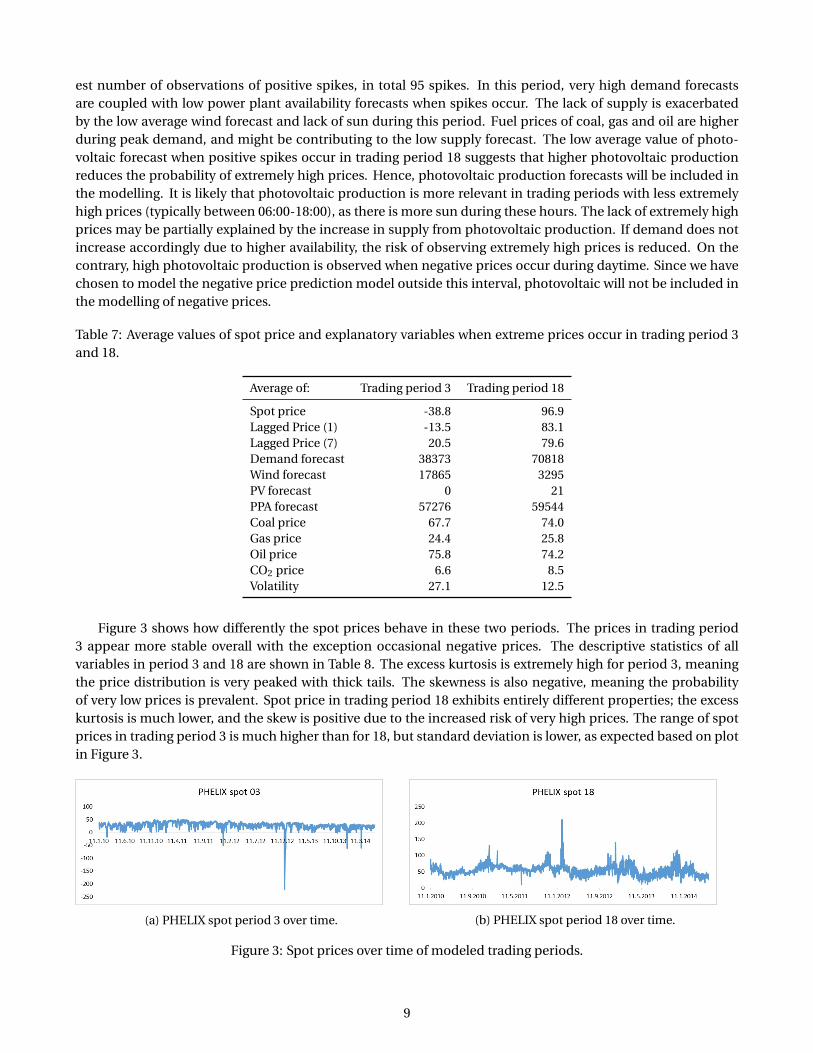
est number of observations of positive spikes, in total 95 spikes. In this period, very high demand forecastsare coupled with low power plant availability forecasts when spikes occur. The lack of supply is exacerbatedby the low average wind forecast and lack of sun during this period. Fuel prices of coal, gas and oil are higherduring peak demand, and might be contributing to the low supply forecast. The low average value of photo-voltaic forecast when positive spikes occur in trading period 18 suggests that higher photovoltaic productionreduces the probability of extremely high prices. Hence, photovoltaic production forecasts will be included inthe modelling. It is likely that photovoltaic production is more relevant in trading periods with less extremelyhigh prices (typically between 06:00-18:00), as there is more sun during these hours. The lack of extremely highprices may be partially explained by the increase in supply from photovoltaic production. If demand does notincrease accordingly due to higher availability, the risk of observing extremely high prices is reduced. On thecontrary, high photovoltaic production is observed when negative prices occur during daytime. Since we havechosen to model the negative price prediction model outside this interval, photovoltaic will not be included inthe modelling of negative prices.

Table 7: Average values of spot price and explanatory variables when extreme prices occur in trading period 3and 18.

Average of: Trading period 3 Trading period 18

Spot price -38.8 96.9Lagged Price (1) -13.5 83.1Lagged Price (7) 20.5 79.6Demand forecast 38373 70818Wind forecast 17865 3295PV forecast 0 21PPA forecast 57276 59544Coal price 67.7 74.0Gas price 24.4 25.8Oil price 75.8 74.2CO2 price 6.6 8.5Volatility 27.1 12.5

Figure 3 shows how differently the spot prices behave in these two periods. The prices in trading period3 appear more stable overall with the exception occasional negative prices. The descriptive statistics of allvariables in period 3 and 18 are shown in Table 8. The excess kurtosis is extremely high for period 3, meaningthe price distribution is very peaked with thick tails. The skewness is also negative, meaning the probabilityof very low prices is prevalent. Spot price in trading period 18 exhibits entirely different properties; the excesskurtosis is much lower, and the skew is positive due to the increased risk of very high prices. The range of spotprices in trading period 3 is much higher than for 18, but standard deviation is lower, as expected based on plotin Figure 3.

(a) PHELIX spot period 3 over time. (b) PHELIX spot period 18 over time.

Figure 3: Spot prices over time of modeled trading periods.

9

Table 8: Descriptive statistics for all explanatory variables (except volatility) for trading period 3 and 18.

Descriptive statistics period 3

Spot price Lagged price (t-1) Lagged price (t-7) Demand forecast Wind Forecast

Mean 27.35 27.26 27.33 43 259.42 5 149.61Std.Dev 14.46 14.53 14.53 5 165.90 4 206.47Min -221.94 -221.94 -221.94 29 201.00 286.16Max 51.08 51.08 51.08 59 149.00 24 525.45Skew -6.21 -6.12 -6.13 0.17 1.63Excess kurtosis 89.37 87.45 87.57 -0.25 2.91

PV Forecast PPA Forecast Coal price Gas price Oil price CO2 price

Mean 0.11 55 128.20 71.28 23.25 74.22 9.33Std.Dev 0.53 4 898.73 11.60 4.10 4.75 4.34Min - 40 015.50 51.49 11.15 61.03 2.48Max 4.52 64 168.50 99.02 39.50 83.78 16.84Skew 5.39 -0.26 0.23 -0.63 -0.73 0.29Excess kurtosis 29.87 -0.78 -1.08 0.96 -0.31 -1.47

Descriptive statistics period 18

Spot price Lagged price (t-1) Lagged price (t-7) Demand forecast Wind Forecast

Mean 55.02 55.02 54.91 60 466.70 5 452.92Std.Dev 16.83 16.83 16.85 8 050.92 4 435.30Min 10.33 10.33 7.62 38 192.00 290.63Max 210.00 210.00 210.00 79 019.00 24 448.44Skew 1.52 1.52 1.51 -0.21 1.46Excess kurtosis 8.34 8.34 8.35 -0.60 2.12

PV Forecast PPA Forecast Coal price Gas price Oil price CO2 price

Mean 1342.10 55 128.25 71.26 23.25 74.21 9.33Std.Dev 1682.02 4 897.20 11.61 4.10 4.76 4.34Min - 40 015.50 51.49 11.15 61.03 2.48Max 7120.10 64 168.50 99.02 39.50 83.78 16.84Skew 1.18 -0.26 0.23 -0.64 -0.73 0.29Excess kurtosis 0.36 -0.77 -1.08 0.95 -0.31 -1.47

4.4 Model design and evaluation

We will be using a standard logit model to investigate the relationship between the fundamental factors andspike occurrences for the same trading period in the following day.

To test the model prediction ability we will use in-sample tests on the modelled data sample, as well astesting the estimated models on data from other similar trading periods as an out-of-sample test.

The in-sample test assesses the ability of the models to truly and falsely predict extreme price occurrences.The probability cutoff value for prediction of an occurrence is commonly set to 50% in most software packages,where estimated probabilities at or above the cutoff are considered occurrences of extreme prices. Adjusting thethreshold may make the models more useful, as it is not given that a 50% threshold is the most appropriate forelectricity spot markets. Failure to forecast a spike is more detrimental to profits for many market participants –particularly retailers that purchase power at the unregulated market spot price, as argued by Christensen et al.(2012). Consequently, false predictions are preferred over failure to predict, and the cut-off may be set lower formodels predicting positive spikes. The chosen cutoff value strongly depends on the purpose of the forecaster,and will be a trade-off between the costs of not detecting a spike versus falsely forecasting one (Eichler et al.(2013)). We argue for evaluating prediction results of the estimated models with different cutoffs, to get a morecomplete picture of the predictive power.

If the probability of extremely high prices is high, the bidders can attempt to increase profits by increasingtheir bids, or ramping up production in time to increase volume in those trading periods. For negative price

10

occurrences the dynamics might be different, as there is a trade-off between continuing operations at a lossversus incurring ramping down/shut-down and ramping up/start-up costs. For these producers it might bemore relevant knowing the probability of the magnitude of the low price, which a logit model is unable to do.The cut-off probability for evaluating the prediction ability for negative prices might therefore benefit from ahigher cut-off than the model for positive spikes. What is defined as an occurrence in the input to the logitmodeling is a positive spike for time period 18, and price below zero for time period 3. The threshold can bevaried to test the model performance with different extreme price specifications, as long as there are sufficientlymany occurrences to estimate a robust model.

5 Results and Discussion

5.1 Estimated logit models

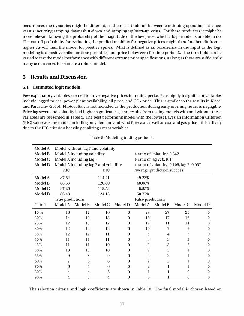
Few explanatory variables seemed to drive negative prices in trading period 3, as highly insignificant variablesinclude lagged prices, power plant availability, oil price, and CO2 price. This is similar to the results in Kieseland Paraschiv (2015). Photovoltaic is not included as the production during early morning hours is negligible.Price lag seven and volatility had higher significances, and results from testing models with and without thesevariables are presented in Table 9. The best performing model with the lowest Bayesian Information Criterion(BIC) value was the model including only demand and wind forecast, as well as coal and gas price – this is likelydue to the BIC criterion heavily penalizing excess variables.

Table 9: Modeling trading period 3.

Model A Model without lag 7 and volatilityModel B Model A including volatility t-ratio of volatility: 0.342Model C Model A including lag 7 t-ratio of lag 7: 0.161Model D Model A including lag 7 and volatility t-ratio of volatility: 0.105, lag 7: 0.057

AIC BIC Average prediction success

Model A 87.52 114.41 49.23%Model B 88.53 120.80 48.08%Model C 87.26 119.53 48.85%Model D 86.48 124.13 50.77%

True predictions False predictionsCutoff Model A Model B Model C Model D Model A Model B Model C Model D

10 % 16 17 16 0 29 27 25 020% 14 13 13 0 16 17 16 025% 12 13 12 0 12 11 14 030% 12 12 12 0 10 7 9 035% 12 12 11 0 5 4 7 040% 11 11 11 0 3 3 3 045% 11 11 10 0 2 3 2 050% 10 10 10 0 2 3 1 055% 9 8 9 0 2 2 1 060% 7 6 8 0 2 2 1 070% 6 5 6 0 2 1 1 080% 4 4 5 0 1 1 0 090% 4 3 4 0 0 1 0 0

The selection criteria and logit coefficients are shown in Table 10. The final model is chosen based on

11

relatively low BIC/AIC, as well as the exclusion of insignificant and collinear variables.

5.2 Discussion on estimated coefficients

Coefficient estimates, as shown in Table 10, are reasonable for both models. In trading period 3, the negativecoefficient of demand implies that high demand reduces the probability of a negative price, while high windproduction increases the probability and thus has a positive coefficient. This is in accordance with previouslyobserved and described market dynamics. Volatility is insignificant in the estimated model for trading period3, suggesting that negative prices do not primarily occur in volatile periods. High fuel prices seem to reduce theprobability of observing negative day-ahead prices. This might be explained by producers being more conser-vative when trading on the power exchange, and preferring shutting down or ramping down production ratherthan continuing operation at a higher loss due to high fuel prices. Consequently, cheap fuel drives produc-ers to rather continue production at negative prices as the opportunity cost of doing so is lower than reducingoutput/shutting down.

Trading period 18 shows different dynamics from period 3; demand forecast coefficient is positive as highdemand is seen in concordance with increased probability of extremely high prices. A higher level of windproduction, on the other hand, reduces the probability of positive spikes. Spikes tend to occur in daily blocks,and it is thus expected that the lagged price coefficients are significant and positive. We note that the first pricelag coefficient is approximately twice as high as for lag seven, meaning the price of the previous day is weighedmore than the weekly pattern. Volatility also has a positive coefficient, which is reasonable as spikes tend tooccur in highly volatile periods. High gas price is a natural driver behind extremely high prices, as gas is relatedto peak supply in the day-ahead market. All supply parameters have negative coefficients, as it is reasonablethat high levels of supply will decrease the chance of positive price spikes.

Table 10: Estimated logit coefficients of model trading period 3 and 18.

AIC 87.52 AIC 302.95BIC 114.41 BIC 351.37Logit coefficients (period 3) Logit coefficients (period 18)

Constant 102.67*** Constant -140.135***

Lagged price (1) Lagged price (1) 0.0334191***

Lagged price (7) Lagged price (7) 0.016962**

Demand forecast -13.4864*** Demand forecast 21.7591***

Wind forecast 7.02236*** Wind forecast -1.58368***

PV forecast PV forecast -2.37763**

PPA Forecast PPA Forecast -10.4955***

Coal -4.03566* CoalGas -3.83327** Gas 6.14538***

Vol Vol 0.127951***

* 10% level of significance ** 5% level of significance *** 1% level of significance

5.3 Evaluation of model performance

When testing the model performance we use the definitions from (Zhao et al. (2007a)) and divide observationsinto four categories: true positive (TP), false positive (FP), true negative (TN) and false negative (FN)

A good prediction model should be highly accurate, thus the value of Equation 1 should be as high as possi-ble. A high prediction accuracy is often obtained at the expense of the confidence level, as defined in Equation2. A high prediction confidence level means the spike forecast is credible. An ideal forecasting model achieves

12

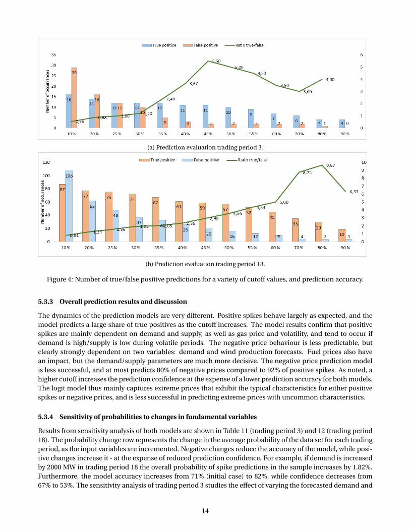
both high accuracy and good confidence simultaneously, but a trade-off is normally required. In-sample modelpredictions results of both trading periods are shown in Figure 4.

Pr edi ct i on_accur ac y = T P

T P +F N(1)

Pr edi ct i on_con f i dence = T P

T P +F P(2)

5.3.1 Trading period 3 prediction results

At the commonly applied cutoff of 50% probability, the model predicts 50% of the negative prices that occurred(true positives), with a confidence of 83%, as shown in Figure 4a. Depending on the cost of failing to predict anegative price, the cutoff can be lowered at the expense of more false positive predictions. At the lowest testedcutoff of 10%, the estimated model predicts 16 (80%) of true positive occurrences, in addition to 29 false pos-itives at a confidence of 36%. At higher cutoffs the model is close to 100% accurate. False negatives exhibit acombination of low wind forecasts compared to the forecasts observed with true positives, and high demandrelative to the true positive. False positives have common characteristics of demand well below the averageof trading period 3 (Table 8), combined with high wind production relative to the true negatives. Fuel pricestend to be low when false positives are predicted, which partially explains the incorrect model predictions. Notsurprisingly, true negatives with the lowest probabilities tend to have highly different characteristics comparedto true positives: average/high demand, and low/average wind production forecast. The data points with prob-abilities larger than zero but below lowest cutoff of 10% tend to have either lower than average demand, orhigher than average wind production. The analysis implies that negative prices that exhibit typical features forthe modelled trading period are easily captured, but that it is more challenging predicting the negative priceoccurrences that exhibit uncommon characteristics.

5.3.2 Trading period 18 prediction results

At the standard cutoff value of 50%, the model is 60% accurate, and predicts 57 true positives as well as 16 falsepositives, as shown in Figure 4b. Higher cutoffs reduce the number of false positives relative to true positivesas cutoff increases, implying that higher cutoffs make the estimated conditional probability more trustworthyin terms of avoiding false positive spike predictions. The chosen cutoff depends on user preference; if theopportunity cost of a false spike is significantly lower than for a missed true spike, a lower cutoff is beneficial.With a cutoff of 10%, the model predicts 87 out of 95 spikes (91.58%). The false negatives are predicted when thephotovoltaic forecast is well above average of the spikes that occurred during period 18 (Table 7). Demand/windforecasts are slightly lower/higher than the average of the spike occurrences, but still above/below average ofthe entire period (Table 8). The false negatives also tend to have much lower lagged prices that the averagefor spike occurrences. The lagged prices are, in some cases, lower than the average lagged prices of period 18.Volatility estimates are also quite low for false negatives, implying not all spikes occur in volatile periods. Falsepositives, on the other hand, exhibit some typical characteristics of true spikes; the lagged prices are far aboveaverage, the demand is high and supply low, volatility is high, and fuel prices tend to be above average of thatperiod. True negative observations exhibit low lagged prices, low demands, and in some cases high forecastedproduction from renewable sources. True negative observations with probabilities below and close to 10%typically have demand forecasts well above average of the trading period, as well as quite low production fromrenewable sources. Interestingly, the gas price was above average, implying that peak power plants were notcheaper to run during these periods. The logit model may struggle to capture the first spike, as the lagged priceis not necessarily high. Conversely, it may also falsely predict spikes following a daily blocks of spikes in highlyvolatile periods, and is unable adjust immediately to a lower price period that follows. However, the modeleasily captures those occurrences that exhibit typical features, and thus identifies the majority of occurrences.

13

(a) Prediction evaluation trading period 3.

(b) Prediction evaluation trading period 18.

Figure 4: Number of true/false positive predictions for a variety of cutoff values, and prediction accuracy.

5.3.3 Overall prediction results and discussion

The dynamics of the prediction models are very different. Positive spikes behave largely as expected, and themodel predicts a large share of true positives as the cutoff increases. The model results confirm that positivespikes are mainly dependent on demand and supply, as well as gas price and volatility, and tend to occur ifdemand is high/supply is low during volatile periods. The negative price behaviour is less predictable, butclearly strongly dependent on two variables: demand and wind production forecasts. Fuel prices also havean impact, but the demand/supply parameters are much more decisive. The negative price prediction modelis less successful, and at most predicts 80% of negative prices compared to 92% of positive spikes. As noted, ahigher cutoff increases the prediction confidence at the expense of a lower prediction accuracy for both models.The logit model thus mainly captures extreme prices that exhibit the typical characteristics for either positivespikes or negative prices, and is less successful in predicting extreme prices with uncommon characteristics.

5.3.4 Sensitivity of probabilities to changes in fundamental variables

Results from sensitivity analysis of both models are shown in Table 11 (trading period 3) and 12 (trading period18). The probability change row represents the change in the average probability of the data set for each tradingperiod, as the input variables are incremented. Negative changes reduce the accuracy of the model, while posi-tive changes increase it - at the expense of reduced prediction confidence. For example, if demand is increasedby 2000 MW in trading period 18 the overall probability of spike predictions in the sample increases by 1.82%.Furthermore, the model accuracy increases from 71% (initial case) to 82%, while confidence decreases from67% to 53%. The sensitivity analysis of trading period 3 studies the effect of varying the forecasted demand and

14

wind production, where the increments are varied from zero (initial case) to higher/lower values - the nega-tive 286 MW limit on the wind forecast increment is to avoid a negative production. The overall probability ofpredicting a negative price using the estimated model changes as expected: the change is negative when de-mand increases or wind production decreases, implying a higher demand or lower wind production reducesthe probability of observing negative prices. Oppositely, the probability change is positive if demand decreaseor wind production increases. The number of true and false positive predictions with a cutoff of 50% changeswith the increments, and the change is particularly observable when the wind forecast is strongly increased;the accuracy decreases from 83% to as low as 22% when wind is increased by 7500 MW. We further tested in-crementing the coal and gas prices; the overall probability of predicting a negative price decreased when fuelprices increase, as expected. The model for trading period 3 is mainly sensitive to changes in wind productionforecast.

Table 11: Sensitivity of probability and prediction accuracy due to changes in demand or wind forecast (tradingperiod 3).

Demand forecast changes

Initial case 1000 3000 5000 -1000 -3000 -5000Probability change 0.00% -0.21% -0.55% -0.79% 0.25% 0.90% 1.81%True positive 10 8 5 4 11 13 15False negative 10 12 15 16 9 7 5False positive 2 2 1 0 2 12 20Accuracy 0.50 0.40 0.25 0.20 0.55 0.65 0.75Confidence 0.83 0.80 0.83 1.00 0.85 0.52 0.43

Wind forecast changes

Initial case 500 1500 2500 4000 7500 -286Probability change 0.00% 0.17% 0.59% 1.12% 2.23% 7.14% -0.09%True positive 10 10 11 13 15 19 10False negative 10 10 9 7 5 1 10False positive 2 2 6 13 19 68 2Accuracy 0.50 0.50 0.55 0.65 0.75 0.95 0.50Confidence 0.83 0.83 0.65 0.50 0.44 0.22 0.83

Trading period 18 sensitivity analysis encompasses varying the first lagged price, demand, wind, and pho-tovoltaic forecast. The variables are chosen because they are the most influential in the model, and due to thefocus on renewable energy source effects on extreme prices. Incrementing the lagged price did not stronglyinfluence the spike probability for increments up to 20, implying that rather extreme changes are needed tosignificantly increase the spike probability. Increasing the wind forecast reduced the accuracy of the model,however, the marginal reduction was clearly decreasing with increasing increment. Changing the demand hada large impact on the estimated probability; particularly positive increments had a strong effect, as predic-tion accuracy increased and confidence decreased. It is noteworthy that the change in probability was closeto linear as the positive increment increased (for increments up to 5000 MW). Gradually increasing the photo-voltaic forecast had a large impact on the spike predictions: the accuracy was reduced, as even small positiveincrements strongly reduced the probability of predicting spikes. Consequently, the model is quite sensitive tochanges in input that are close to the average value of each case of spike/no spike, except in the case of demandwhere the magnitude of change increased approximately linearly even for high, positive increments.

Demand is much more influential in the trading period 18 compared to period 3, and the effect of incremen-tal changes also differs: an increase in demand lowers accuracy and increases confidence for trading period 3,while in trading period 18 a higher demand increases accuracy and reduces confidence - as expected. Wind isalso, somewhat more surprising, more influential in the model for trading period 18 when considering proba-

15

Table 12: Sensitivity of probability and prediction accuracy due to changes in fundamental variables (tradingperiod 18).

Lagged price 1 changes Demand changes

Initial case 10 20 -10 -20 2000 5000 -2000 -5000Probability change 0.00% 0.93% 1.98% -1.57% -0.43% 1.82% 5.19% -1.49% -3.15%True positive 57 60 67 36 55 67 78 37 26False negative 38 35 28 59 40 28 17 58 69False positive 16 22 33 7 12 33 68 7 3Accuracy 0.60 0.63 0.71 0.38 0.58 0.71 0.82 0.39 0.27Confidence 0.78 0.75 0.73 0.82 0.83 0.67 0.53 0.84 0.90

Wind forecast changes PV forecast changes

Initial case 1000 2000 3000 4000 500 1000 1500 2000Probability change 0.00% -1.23% -1.99% -2.51% -2.91% -2.53% -4.06% -4.93% -5.39%True positive 57 39 35 30 26 30 18 8 6False negative 38 56 60 65 69 65 77 87 89False positive 16 7 3 3 2 4 1 0 0Accuracy 0.60 0.41 0.37 0.32 0.27 0.32 0.19 0.08 0.06Confidence 0.78 0.73 0.67 0.84 0.82 0.88 0.95 1.00 1.00

bility percentage changes. This may be due to the lower average wind production during this period, causingthe increments to have a larger impact. It may also imply the model for positive spikes is more sensitive, whichmay be explained by the larger number of variables or more extreme price occurrences as basis for modeling(Figure 2). The results from the sensitivity analysis yield expected results, and further confirms the main driversbehind extremely high and low prices.

5.3.5 Out-of-sample test

A comparison of trading period 3 with period 2 and 4 shows that these periods exhibit many similarities. As seenin Table 13, there is a similar number of negative price occurrences; 20, 20, and 14 observations for period 2, 3,and 4 respectively. The average negative spot prices were quite low in all cases, although the absolute magnitudewas slightly higher for period 4. The demand forecasts and wind forecasts average values are similar betweenthe three periods, implying that the price formation dynamics are similar. For the entire set of values observedin these periods, the characteristics are even more similar; the average spot price, demand forecast and averagewind forecast are essentially the same, and photovoltaic forecast is zero for these night-time periods. Pricesof fuel and CO2 are given on a per-day basis, as noted in Table 2, and will thus have the same impact in themodeling of these periods. Trading period 18 exhibits much of the same characteristics as period 17 and 19,as seen in Table 14. Table 15 shows that the number of spikes is higher for trading period 18 (95 observations),relative to 64 and 60 respectively for period 17 and 19. The average spot price and average demand forecastfor spike occurrences is slightly lower for period 19. In addition, the average photovoltaic forecast is very lowfor trading period 19, and hardly has an impact on extremely high prices. Photovoltaic forecasts are on averagehigher for period 17, as there naturally is more sunlight during this period, and this constitutes the largestdifference compared with period 18. However, when spikes occur the difference is insignificant.

The general price formation dynamics for trading period 2, 3 and 4 are quite similar, and the extreme pricesappear to have similar drivers. For trading period 18, the implication is that period 17 is very similar and likely tobehave similarly in the tails. Although each hourly time series is unique, there are strong similarities in adjacenttrading periods. Because of the lack of sufficiently many normal range and extreme price observations in eachtrading period, conducting a traditional out-of-sample test for the modelled trading periods was challenging.We therefore use data from trading period 2 and 4 to test the model for predicting negative prices, and tradingperiod 17 data to test the model for predicting positive spikes.

16

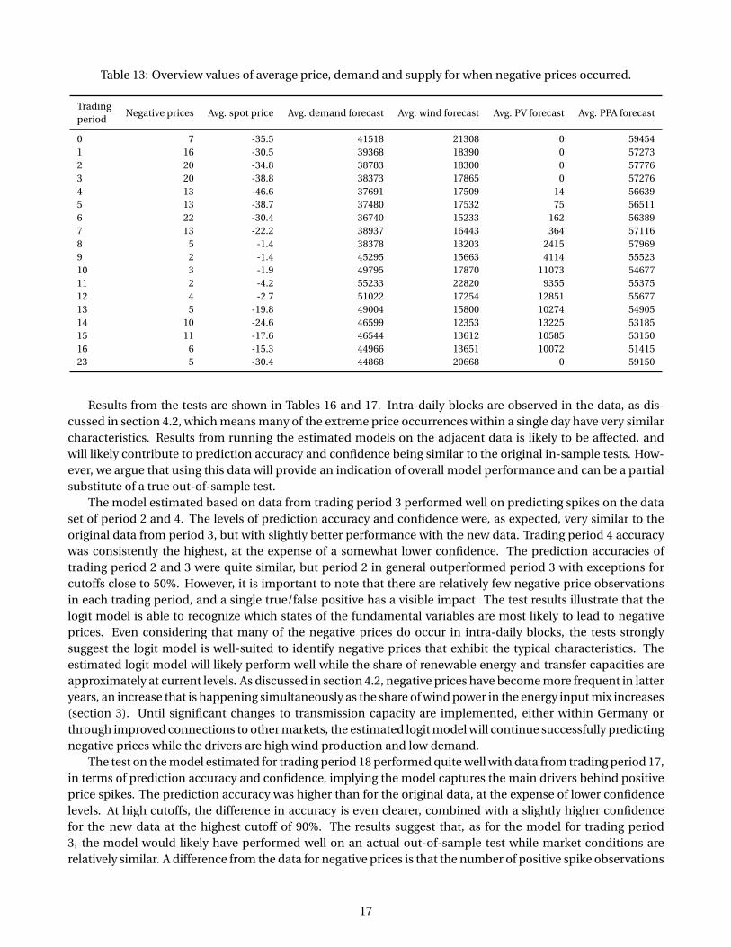
Table 13: Overview values of average price, demand and supply for when negative prices occurred.

Tradingperiod

Negative prices Avg. spot price Avg. demand forecast Avg. wind forecast Avg. PV forecast Avg. PPA forecast

0 7 -35.5 41518 21308 0 594541 16 -30.5 39368 18390 0 572732 20 -34.8 38783 18300 0 577763 20 -38.8 38373 17865 0 572764 13 -46.6 37691 17509 14 566395 13 -38.7 37480 17532 75 565116 22 -30.4 36740 15233 162 563897 13 -22.2 38937 16443 364 571168 5 -1.4 38378 13203 2415 579699 2 -1.4 45295 15663 4114 5552310 3 -1.9 49795 17870 11073 5467711 2 -4.2 55233 22820 9355 5537512 4 -2.7 51022 17254 12851 5567713 5 -19.8 49004 15800 10274 5490514 10 -24.6 46599 12353 13225 5318515 11 -17.6 46544 13612 10585 5315016 6 -15.3 44966 13651 10072 5141523 5 -30.4 44868 20668 0 59150

Results from the tests are shown in Tables 16 and 17. Intra-daily blocks are observed in the data, as dis-cussed in section 4.2, which means many of the extreme price occurrences within a single day have very similarcharacteristics. Results from running the estimated models on the adjacent data is likely to be affected, andwill likely contribute to prediction accuracy and confidence being similar to the original in-sample tests. How-ever, we argue that using this data will provide an indication of overall model performance and can be a partialsubstitute of a true out-of-sample test.

The model estimated based on data from trading period 3 performed well on predicting spikes on the dataset of period 2 and 4. The levels of prediction accuracy and confidence were, as expected, very similar to theoriginal data from period 3, but with slightly better performance with the new data. Trading period 4 accuracywas consistently the highest, at the expense of a somewhat lower confidence. The prediction accuracies oftrading period 2 and 3 were quite similar, but period 2 in general outperformed period 3 with exceptions forcutoffs close to 50%. However, it is important to note that there are relatively few negative price observationsin each trading period, and a single true/false positive has a visible impact. The test results illustrate that thelogit model is able to recognize which states of the fundamental variables are most likely to lead to negativeprices. Even considering that many of the negative prices do occur in intra-daily blocks, the tests stronglysuggest the logit model is well-suited to identify negative prices that exhibit the typical characteristics. Theestimated logit model will likely perform well while the share of renewable energy and transfer capacities areapproximately at current levels. As discussed in section 4.2, negative prices have become more frequent in latteryears, an increase that is happening simultaneously as the share of wind power in the energy input mix increases(section 3). Until significant changes to transmission capacity are implemented, either within Germany orthrough improved connections to other markets, the estimated logit model will continue successfully predictingnegative prices while the drivers are high wind production and low demand.

The test on the model estimated for trading period 18 performed quite well with data from trading period 17,in terms of prediction accuracy and confidence, implying the model captures the main drivers behind positiveprice spikes. The prediction accuracy was higher than for the original data, at the expense of lower confidencelevels. At high cutoffs, the difference in accuracy is even clearer, combined with a slightly higher confidencefor the new data at the highest cutoff of 90%. The results suggest that, as for the model for trading period3, the model would likely have performed well on an actual out-of-sample test while market conditions arerelatively similar. A difference from the data for negative prices is that the number of positive spike observations

17

Table 14: Overview values of average price, demand and supply for all trading periods.

Tradingperiod

Avg. spot price Avg. demand forecast Avg. wind forecast Avg. PV forecast Avg. PPA forecast

0 35.1 46027 5241 0 551461 31.8 44153 5205 0 551462 29.2 43213 5173 0 551463 27.4 43284 5147 0 551464 27.8 44159 5134 5 551485 31.1 46138 5109 59 551456 38.0 51135 5098 318 551467 46.9 56028 5092 1150 551468 50.4 58922 5086 2696 551469 50.6 60365 5121 4616 5514610 50.0 61822 5190 6365 5514611 50.3 63153 5313 7593 5514612 47.9 62527 5445 8097 5514613 45.3 61365 5555 7898 5514614 43.4 60065 5613 7079 5514615 42.8 59181 5611 5746 5514616 43.7 58638 5578 4144 5514617 49.7 59707 5529 2600 5514618 55.0 60493 5453 1336 5514619 55.0 60074 5362 511 5514620 50.4 57723 5292 103 5514621 45.8 55524 5269 8 5514622 44.7 53432 5260 0 5514623 38.3 49301 5249 0 55146

decreases over time, based on the latest trend in the data (section 4.2).As previously mentioned, the share of renewable energy source input will probably increase in coming

years, while authorities focus on strengthening the grid. The effects of these changes are not yet known, buta likely consequence is that the dynamics in the day-ahead electricity market change. Consequently, extremelyhigh prices may be more or less frequent, and some drivers may become increasingly important. If, for exam-ple, storage opportunities are cost-effectively introduced into the market, the intermittent nature of wind andphotovoltaic power plants will have less impact. In this case high demand forecasts may be a more influentialdriver behind positive price spikes. For negative prices, this may imply the frequency would decrease, as theexcess energy produced to some degree could be stored when the supply excessively exceeds demand.

5.4 Effect of renewable energy sources as explanatory variables

When removing wind as explanatory variable from the model for trading period 3, it performs significantlyworse. The results of the modeling are displayed in Table 20, and show that the model performed worse on allcriteria, including AIC, BIC, and prediction accuracy/confidence. The finding confirms that high wind produc-tion is the main driver behind negative prices during nightly trading periods. Coefficients of variables are lowerin the model without wind forecasts included, as shown in Table 19. The model estimation is unable to make asufficiently powerful logit model for predicting negative prices if wind forecasts are not included.

18

Table 15: Overview values of average price, demand and supply for when positive spikes occurred.

Tradingperiod

Positive spikes Avg. spot price Avg. demand forecast Avg. wind forecast Avg. PV forecast Avg. PPA forecast

7 24 93.7 66414 2460 361 589628 36 94.8 67121 2425 1757 576699 22 93.4 69392 2805 2946 5790310 17 93.0 71744 2936 3084 5935511 23 89.8 70982 2673 5183 5663912 11 89.7 71764 2249 5138 5823113 7 88.3 71468 2173 4970 5908314 3 94.5 70783 2077 3101 6010315 4 89.1 71528 2615 1577 6046416 12 88.3 70637 2166 406 6013217 64 95.4 72123 3378 57 5946818 95 96.9 70818 3295 21 5954419 60 91.8 68067 3409 16 5875120 7 95.2 67368 4295 0 5852121 1 94.9 67678 2032 0 6057122 1 79.7 66366 1892 0 60571

Table 18: Estimated coefficients with/without wind/photovoltaic forecast for trading period 18.

Coefficient Model A Model B Model C Model D

Constant -140.135*** -140.78*** -252.715*** -205.421***

Lagged price (1) 0.0334191*** 0.0448175*** 0.0403652*** 0.0491872***

Lagged price (7) 0.016962** 0.0149543** 0.0214126*** 0.01178986***

Demand forecast 21.7591*** 17.315*** 25.2775*** 19.3292***

Wind forecast -1.58368*** 0 -1.49916 0PV forecast -2.37763** -1.63813* 0 0PPA Forecast -10.4955*** -6.91747** -3.95059 -3.1017Gas 6.14538*** 5.30204*** 6.01466*** 5.14221***

Volatility 0.127951*** 0.108976*** 0.136867*** 0.118718***

* for 10% level of significance ** for 5% level of significance*** for 1% level of significance

Table 19: Estimated coefficients with/without wind forecast for trading period 3.

Coefficient Model A (with wind) Model B (without wind)

Constant 102.67*** 103.734***

Demand forecast -13.4864*** -9.11115***

Wind forecast 7.02236***

Coal price -4.03566* -2.76219*

Gas price -3.83327** 0.0611909

* for 10% level of significance ** for 5% level of significance*** for 1% level of significance

For trading period 18, the prediction results of models estimated without the renewable energy sources aresignificantly less accurate than the basic model. As seen in Table 21, Model A clearly has the best predictionaccuracy for price spikes, and in addition has relatively few occurrences of false positives. Model B predicts the

19

Table 16: Prediction results from using estimated model for predicting negative prices on data from tradingperiod 2 and 4.

Data 2 Data 4Cutoff TP FN FP Accuracy Confidence TP FN FP Accuracy Confidence

10% 19 1 30 0.95 0.39 10 3 27 0.77 0.2720% 17 3 13 0.85 0.57 10 3 15 0.77 0.4025% 14 6 13 0.70 0.52 10 3 11 0.77 0.4830% 13 7 9 0.65 0.59 10 3 9 0.77 0.5335% 12 8 7 0.60 0.63 9 4 6 0.69 0.6040% 11 9 5 0.55 0.69 9 4 4 0.69 0.6945% 10 10 2 0.50 0.83 8 5 4 0.62 0.6750% 9 11 2 0.45 0.82 8 5 4 0.62 0.6755% 9 11 1 0.45 0.90 7 6 3 0.54 0.7060% 8 12 1 0.40 0.89 6 7 3 0.46 0.6770% 6 14 1 0.30 0.86 5 8 3 0.38 0.6380% 4 16 1 0.20 0.80 4 9 1 0.31 0.8090% 4 16 0 0.20 1.00 2 11 0 0.15 1.00

Table 17: Prediction results from using estimated model for predicting spikes on data from trading period 17.

Cutoff TP FN FP Prediction accuracy Prediction confidence

10% 60 3 97 0.95 0.3820% 54 9 58 0.86 0.4825% 52 11 46 0.83 0.5330% 49 14 36 0.78 0.5835% 46 17 31 0.73 0.6040% 44 19 27 0.70 0.6245% 41 22 21 0.65 0.6650% 39 24 15 0.62 0.7255% 37 26 14 0.59 0.7360% 36 27 12 0.57 0.7570% 32 31 7 0.51 0.8280% 26 37 4 0.41 0.8790% 18 45 2 0.29 0.90

highest number of false positives, but performs better than model D on predicting true positives. We concludethat removing the renewable energy sources as explanatory variables makes the logit models less able to suc-cessfully predict spike occurrences. Coefficients of estimated models are relatively similar for all models, andare given in Table 18. The lagged price coefficients are somewhat higher for Model B and C, indicating first pricelag is weighed more relative to the model excluding renewable supply forecast. This implies the price the pre-vious day has a larger impact on predicted spike probability when renewable energy sources are not included.Consequently, estimated models rely more on the lagged price, and may be less able to predict the first spike ina potential series of spikes for trading period 18 over several days.

5.5 Robustness Analysis

As discussed in section 4, determining the spike threshold is important to be able to estimate a logit model.Table 22 shows how the number of spike occurrences changes for different thresholds. Estimating models usingvarious spike thresholds yields the coefficients shown in Table 23. Lagged prices, demand forecast and supply

20

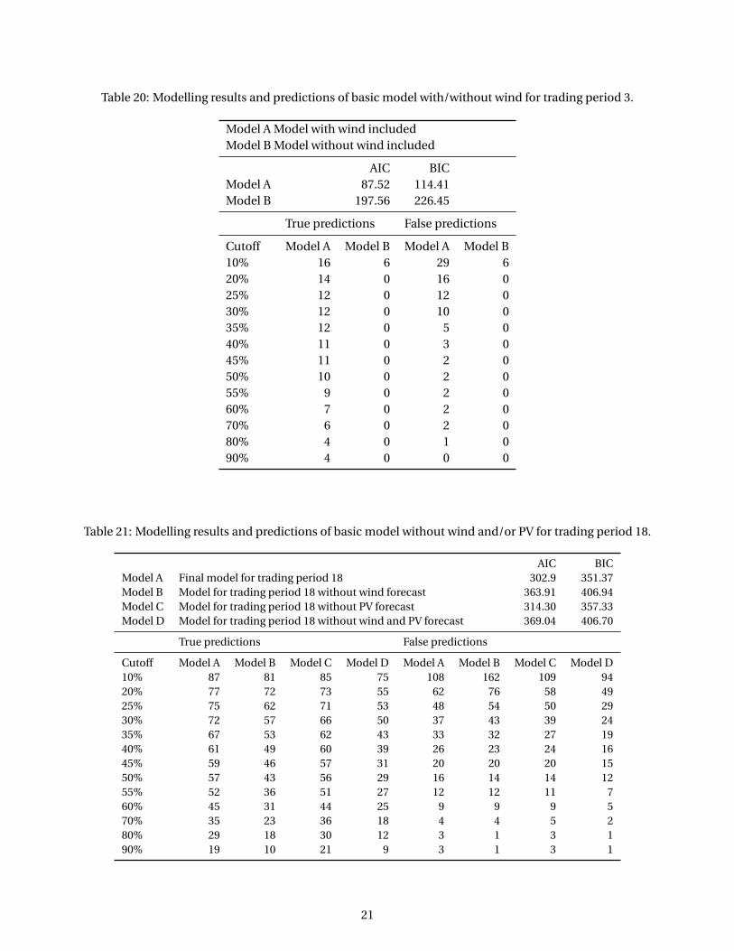
Table 20: Modelling results and predictions of basic model with/without wind for trading period 3.

Model A Model with wind includedModel B Model without wind included

AIC BICModel A 87.52 114.41Model B 197.56 226.45

True predictions False predictions

Cutoff Model A Model B Model A Model B10% 16 6 29 620% 14 0 16 025% 12 0 12 030% 12 0 10 035% 12 0 5 040% 11 0 3 045% 11 0 2 050% 10 0 2 055% 9 0 2 060% 7 0 2 070% 6 0 2 080% 4 0 1 090% 4 0 0 0

Table 21: Modelling results and predictions of basic model without wind and/or PV for trading period 18.

AIC BICModel A Final model for trading period 18 302.9 351.37Model B Model for trading period 18 without wind forecast 363.91 406.94Model C Model for trading period 18 without PV forecast 314.30 357.33Model D Model for trading period 18 without wind and PV forecast 369.04 406.70

True predictions False predictions

Cutoff Model A Model B Model C Model D Model A Model B Model C Model D10% 87 81 85 75 108 162 109 9420% 77 72 73 55 62 76 58 4925% 75 62 71 53 48 54 50 2930% 72 57 66 50 37 43 39 2435% 67 53 62 43 33 32 27 1940% 61 49 60 39 26 23 24 1645% 59 46 57 31 20 20 20 1550% 57 43 56 29 16 14 14 1255% 52 36 51 27 12 12 11 760% 45 31 44 25 9 9 9 570% 35 23 36 18 4 4 5 280% 29 18 30 12 3 1 3 190% 19 10 21 9 3 1 3 1

21

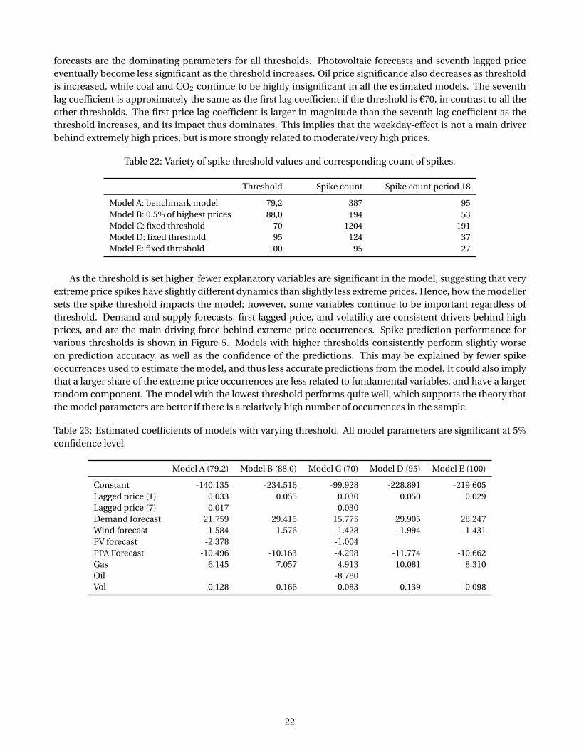
forecasts are the dominating parameters for all thresholds. Photovoltaic forecasts and seventh lagged priceeventually become less significant as the threshold increases. Oil price significance also decreases as thresholdis increased, while coal and CO2 continue to be highly insignificant in all the estimated models. The seventhlag coefficient is approximately the same as the first lag coefficient if the threshold is €70, in contrast to all theother thresholds. The first price lag coefficient is larger in magnitude than the seventh lag coefficient as thethreshold increases, and its impact thus dominates. This implies that the weekday-effect is not a main driverbehind extremely high prices, but is more strongly related to moderate/very high prices.

Table 22: Variety of spike threshold values and corresponding count of spikes.

Threshold Spike count Spike count period 18

Model A: benchmark model 79,2 387 95Model B: 0.5% of highest prices 88,0 194 53Model C: fixed threshold 70 1204 191Model D: fixed threshold 95 124 37Model E: fixed threshold 100 95 27

As the threshold is set higher, fewer explanatory variables are significant in the model, suggesting that veryextreme price spikes have slightly different dynamics than slightly less extreme prices. Hence, how the modellersets the spike threshold impacts the model; however, some variables continue to be important regardless ofthreshold. Demand and supply forecasts, first lagged price, and volatility are consistent drivers behind highprices, and are the main driving force behind extreme price occurrences. Spike prediction performance forvarious thresholds is shown in Figure 5. Models with higher thresholds consistently perform slightly worseon prediction accuracy, as well as the confidence of the predictions. This may be explained by fewer spikeoccurrences used to estimate the model, and thus less accurate predictions from the model. It could also implythat a larger share of the extreme price occurrences are less related to fundamental variables, and have a largerrandom component. The model with the lowest threshold performs quite well, which supports the theory thatthe model parameters are better if there is a relatively high number of occurrences in the sample.

Table 23: Estimated coefficients of models with varying threshold. All model parameters are significant at 5%confidence level.

Model A (79.2) Model B (88.0) Model C (70) Model D (95) Model E (100)

Constant -140.135 -234.516 -99.928 -228.891 -219.605Lagged price (1) 0.033 0.055 0.030 0.050 0.029Lagged price (7) 0.017 0.030Demand forecast 21.759 29.415 15.775 29.905 28.247Wind forecast -1.584 -1.576 -1.428 -1.994 -1.431PV forecast -2.378 -1.004PPA Forecast -10.496 -10.163 -4.298 -11.774 -10.662Gas 6.145 7.057 4.913 10.081 8.310Oil -8.780Vol 0.128 0.166 0.083 0.139 0.098

22

(a) Prediction accuracy.

(b) Prediction confidence.

Figure 5: Trading period 18 prediction results for different thresholds.

6 Conclusion and Recommendations for Further Work

The estimated models are able to explain extreme prices quite well, as confirmed by the in-sample test in sec-tions 5.3.1, and 5.3.2 and the out-of-sample test in section 5.3.5). The results suggest that extreme price occur-rences have clear drivers, and that logit models are an appropriate tool for assessing the impacts of fundamentalvariables. Our analysis shows that probability models can identify and quantify these drivers, both for negativeprices and positive spikes, and can thus be a powerful tool contributing to risk management. The benefit of us-ing logit models is that they are easy to estimate and are flexible, as each modeller can customize thresholds todefine extreme prices and change the probability cutoff to adjust the weighing of accuracy versus confidence.The model performance was quite good for all thresholds, with somewhat lower accuracy and confidence forvery high thresholds (€100). Very high thresholds have the drawback of fewer data points for model estimation,and the choice of threshold should balance the need to filter extreme prices from normal range, while ensuringrobust model specification. Thus, a challenge in estimating a robust model in this field is to obtain sufficientlymany data points of extreme price occurrences. This complicates the testing procedure of the model, as out-of-sample tests require enough data points to be credible. In general, as for all probability models estimatedon a data set, the model should and will have the highest predictive power in a market situation similar to theoriginal data sample. Consequently, as the German day-ahead electricity market fundamentals change overtime, as described in Chapter 3, new models should be estimated to ensure good performance.

As initial study of the data suggested, positive spikes and negative prices have very different dynamics andfundamental drivers. In addition, each trading period has unique price dynamics, especially when comparing

23

day/night-time. Positive spikes are mainly observed when demand forecast levels are high and supply fore-casts are low, as well as high lagged price the previous day. The estimated logit model confirms these dynamics,and in addition implies that the weekday effect measured through the seven-day lag is not a very significantdriver behind extreme prices. Negative prices are, on the other hand, driven mainly by wind power combinedwith very low demand. As shown in section 5.4, model performance was poor when wind was not included asfundamental variable. The results imply that negative prices were also not driven by low lagged prices, as wassuggested in the initial data study (section 4.2). The effect of renewable energy sources is clear in the study ofextreme price behaviour. Positive spikes are less frequent if wind/photovoltaic production forecasts are high, asthe spikes occur when production forecasts are low causing demand to exceed supply. The sensitivity analysisof parameters strongly suggests that increased renewable energy production forecasts lower the probabilities ofobserving spikes. Negative prices are strongly dependent on renewable energy, and are most common duringnight as a consequence of high levels of wind production and low demand. Daytime negative prices are seenwhen photovoltaic production forecasts are very high, although these observations are quite few. The nega-tive prices are, on average, much lower during night than during day, implying the effect of renewable energysources is strongest at night.

As a main conclusion, the extreme price behavior in a single trading period is captured well with a logitmodel. Identifying the main drivers behind extreme prices is highly useful in risk management for marketparticipants. The effect of renewable energy sources is clear, and will continue to be important in this market.Intermittency of renewable energy sources is unlikely to decrease in near future, and it is important to usepredictive models that account for these dynamics is important for participants in the electricity spot market.We expect the negative price observations to decrease with future improvements of the transmission gird, asbalance between the power production in the north and power demand in the south is improved.

To further model the occurrences of spikes in the German EPEX market an obvious step is to model thelikely magnitude of the predicted extreme prices. One suggested method is incorporating the binomial logitmodel with a quantile regression. The estimated logit probability may be used as an input to determine whichquantile the price is most likely to be; a 90% logit probability may be used as an indicator that the forecastedprice is in an upper quantile. Another option would be to include the logit probability as a fundamental variablein the quantile regression model, thus utilizing the probability of a spike to forecast the magnitude. An ExtremeValue Theory (EVT) model may be used to more accurately model the tail distribution of prices. A combinedapproach, using a logit model for the probability of spike occurences combined with an EVT model on top forshaping the extreme tails can bring an additional contribution methodologically. For a more comprehensivestudy, the analysis may not be limited to two trading periods, but be estimated for different times of the day.Alternatives are closer analysis of daytime negative prices, as well as morning hours where both negative pricesand positive spikes occur, e.g. trading period 7, 8, and 9. To further improve the estimated logit models accuracyand confidence, a more advanced volatility model, e.g., GARCH, may improve the model fitting.

Testing of the model may be done on different simulated fundamental variable scenarios and correspondingspot price. Demand is strongly seasonal and has clear weekly patterns, while the supply is highly dependenton fuel prices for conventional power plants, as well as weather forecasts. The logit model performance maybe done on the simulated data. Probability of extreme price occurrences in interesting in many markets, notonly the German EPEX, and the methodology may be employed on other markets. This could, for instance, bedone on the Nord Pool or UK APX. Comparisons of extreme price dynamics in these markets may be conducted,to study if spikes are always driven by the same parameters. A possible approach may be studying the energyinput mix and its impact on the extreme price occurrences and magnitude, as well as drivers.

Marcel Prokopczuk and Sjur Westgaard gratefully acknowledge financial support from E.ON Stipendien-fonds.

24

References

Arvesen, Ø., Medbø, V., Fleten, S.-E., Thomasgard, A., and Westgaard, S. (2013). Linepack storage valuationunder price uncertainty. Energy, 52:155–164.

Borovkova, S. and Permana, F. J. (2006). Modelling electricity prices by the potential jump-diffusion. In Stochas-tic Finance, chapter 9. SpringerLink.

Bunn, D., Andresen, A., Chen, D., and Westgaard, S. (Forthcoming 2016). Analysis and forecasting of electricityprice risks with quantile factor models. Energy Journal.

Bunn, D. W. and Karakatsani, N. (2003). Forecasting electricity prices. London Business School, 1.

Byström, H. N. (2005). Extreme value theory and extremely large electricity price changes. International Reviewof Economics & Finance, 14(1):41–55.

Cartea, A. and Figueroa, M. G. (2005). Princing in Electrcity Markets: A Mean Reverting Jump Diffusion Modelwith Seasonality. Applied Mathematical Finance, 12(4):313–335.

Christensen, T., Hurn, A., and Lindsay, K. (2009). It never rains but it pours: modeling the persistence of spikesin electricity prices. Energy Journal, 30(1):25–48.

Christensen, T., Hurn, A., and Lindsay, K. (2012). Forecasting Spikes in Electricity Prices. NCER Working PapersSeries, 70.

Eichler, M., Grothe, O., Manner, H., and Türk, D. (2013). Models for short-term forecasting of spike occurrencesin Australian electricity markets: a comparative study (working paper).

Energiebilanzen, A. (2015). http://www.ag-energiebilanzen.de/. Bruttostromerzeugung in Deutschland von1990 bis 2013 nach EnergietrÀgern. Downloaded on 21/09/2015.

Fanone, E., Gamba, A., and Prokopczuk, M. (2013). The case of negative day-ahead electricity prices. EnergyEconomics, 35:22–34.

Frondel, M., Ritter, N., Schmidt, C. M., and Vance, C. (2010). Economic Impacts from the Promotion of Renew-able Energy Technologies: the German Experience. Energy Policy, 38:4048–4056.

Genoese, F., Genoese, M., and Wietschel, M. (2010). Occurrence of negative prices on the German spot marketfor electrcity and their influence on balancing power markets. IEEE 2010 7th International Conference on theEuropean Energy Market (EEM), pages 1–6.

Hagfors, L. I., Molnar, P., Paraschiv, F., and Westgaard, S. (Forthcoming 2016). Using Quantile Regression toAnalyze the Effect of Renewables on EEX Price Formation (working paper). Journal of Physics, ConferenceSeries.

Higgs, H. and Worthington, A. (2008). Stochastic price modeling of high volatility, mean-reverting, spike-pronecommodities: The Australian wholesale spot electricity market. Energy Economics, 30:3172–3185.

Huisman, R. and de Jong, C. (2003). Option Formulas for Power Prices with Spikes. Energy Power Risk Manage-ment, 7.

Huisman, R., Stradnic, V., and Westgaard, S. (2013). Renewable Energy and Electrcity Prices: Indirect EmpiricalEvidence from Hydro Power. Documents de Treball de I’IEB, 24.

Janczura, J. and Weron, R. (2010). An Empirical comparison of alternate regime-switching models for electricityspot prices. Energy Economics, 32:1059–1073.

25

Karakatsani, N. V. and Bunn, D. W. (2010). Fundamental and behavioural drivers of electricity price volatility.Studies in Nonlinear Dynamics & Econometrics, 14(4).

Kauppi, H. and Saikkonen, P. (2008). Predicting U.S Recessions with Dynamic Binary Response Models. TheReview of Economics and Statistics, 90(4):777–791.

Keles, D., Genoese, M., Möst, D., and Fichtner, W. (2011). Comparison of extended mean-reversion and timeseries models for electricity spot price simulation considering negative prices. Energy Economics, 34:1012–1032.

Kiesel, R. and Paraschiv, F. (2015). Econometric Analysis of 15-Minute Intraday Electricity Prices. University ofSt.Gallen, School of Finance Research Paper No. 2015/21.

Kovacevic, R. M. and Paraschiv, F. (2014). Medium-term planning for thermal Electrcity production. OR Spec-trum, 36(3):723–759.

Lu, X., Dong, Z. Y., and Li, X. (2005). Electricity market price spike forecast with data mining techniques. ElectricPower Systems Research, 73(1):19–29.

Mount, T., Ning, Y., and Chai, X. (2006). Predicting price spikes in electricity markets using a regime-switchingmodel with time-varying parameters. Energy Economics, 28(1):62–80.

Paraschiv, F., Erni, D., and Pietsch, R. (2014). The impact of renewable energies on EEX day-ahead electricityprices. Energy Policy, 73:196–210.

Paraschiv, F., Fleten, S.-E., and Schürle, M. (2015). A Spot-forward model for the electrcity prices with regimeshifts. Energy Economics, 47:142–153.

Paraschiv, F., Hadzi-Mishev, R., and Keles, D. (Forthcoming 2016). Extreme value theory for heavy-tails in elec-tricity prices. Journal of Energy Markets.

Schneider, S. and Schneider, S. (2010). Power Spot Price Models with negative Prices. MPRA paper.

Stevenson, M. J., do Amaral, L. F. M., and Peat, M. (2006). Risk Management and the Role of Spot Price Predic-tions in the Australian Retail Electricity Market. Studies in Nonlinear Dynmaic and Econometrics, 10(3).

Thomas, S., Ramiah, V., Mitchell, H., and Heaney, R. (2011). Seasonal factor and outlier effects in rate of returnon electricity spot prices in Australia’s National Electricity Market. Applied Economics, 43:355–369.

Trück, S., Weron, R., and Wolff, R. (2007). Outlier Treatment and Robust Approaches for Modeling ElectricitySpot Prices. MPRA paper.

Weron, R. (2009). Heavy-tails and regime-switching in Electrcity prices. Mathematical Methods in OperationsResearch, 69(3):457–473.

Weron, R., Bierbrauer, M., and Trück, S. (2004). Modeling electricity prices: jump diffusion and regime switch-ing. Physica A, 336:39–48.

Weron, R. and Misiorek, A. (2005). Forecasting spot electricity prices with time series models. Proceedings of theEuropean Electricity Market EEM-05 Conference, Lodz, pages 133–141.

Zhao, J. H., Dong, Z. Y., and Li, X. (2007a). Electricity market price spike forecasting and decision making. IETGeneration, Transmission & Distribution, 1(4):647–654.

Zhao, J. H., Dong, Z. Y., Li, X., and Wong, K. P. (2007b). A Framework for Electricity Price Spike Analysis WithAdvanced Data Mining Methods. IEEE Transactions on Power Systems, 22(1):377–385.

26