Embed Size (px)
Citation preview

Predictive Modeling Using Logistic Regression
Course Notes

Predictive Modeling Using Logistic Regression Course Notes was developed by William J. E. Potts and Michael J. Patetta. Additional contributions were made by Chris Bond, Jim Georges, Jin Whan Jung, Bob Lucas, and David Schlotzhauer. Editing and Production support was provided by the Curriculum Development and Support Department.
SAS and all other SAS Institute Inc. product or service names are registered trademarks or trademarks of SAS Institute Inc. in the USA and other countries. ® indicates USA registration.
Other brand and product names are trademarks of their respective companies.
The Institute is a private company devoted to the support and further development of its software and related services.
Predictive Modeling Using Logistic Regression Course Notes
Copyright 2002 by SAS Institute Inc., Cary, NC 27513, USA. All rights reserved. Printed in the United States of America. No part of this publication may be reproduced, stored in a retrieval system, or transmitted, in any form or by any means, electronic, mechanical, photocopying, or otherwise, without the prior written permission of the publisher, SAS Institute Inc.
Book code 57700, course code PMLR, prepared date 17May00.

For Your Information iii
Table of Contents
Course Description .............................................................................................................v
Prerequisites......................................................................................................................vi
General Conventions........................................................................................................vii
Chapter 1 Predictive Modeling ...................................................................................1-1
1.1 Introduction ............................................................................................................1-2
1.2 Analytical Challenges ............................................................................................1-9
1.3 Chapter Summary................................................................................................1-14
Chapter 2 Fitting the Model.........................................................................................2-1
2.1 The Model ...............................................................................................................2-2
2.2 Adjustments for Oversampling............................................................................2-16
2.3 Chapter Summary................................................................................................2-27
Chapter 3 Preparing the Input Variables....................................................................3-1
3.1 Missing Values .......................................................................................................3-2
3.2 Categorical Inputs ................................................................................................3-10
3.3 Variable Clustering ..............................................................................................3-21
3.4 Subset Selection ...................................................................................................3-36
3.5 Chapter Summary................................................................................................3-52
Chapter 4 Classifier Performance ..............................................................................4-1
4.1 Honest Assessment ................................................................................................4-2
4.2 Misclassification ...................................................................................................4-17
4.3 Allocation Rules....................................................................................................4-30

iv For Your Information
4.4 Overall Predictive Power .....................................................................................4-36
4.5 Chapter Summary................................................................................................4-41
Chapter 5 Nonlinearities and Interactions .................................................................5-1
5.1 Detection .................................................................................................................5-2
5.2 Polynomials.............................................................................................................5-8
5.3 Multilayer Perceptrons ........................................................................................5-14
5.4 Chapter Summary................................................................................................5-19
Appendix A Additional Resources................................................................................ A-1
A.1 A1 Exercises........................................................................................................... A-2
A.2 A2 Exercise Solutions............................................................................................ A-7
A.3 A3 References ...................................................................................................... A-37
Appendix B Index........................................................................................................... B-1

For Your Information v
Course Description
This course covers predictive modeling using SAS/STAT software with emphasis on the LOGISTIC procedure. The issues and techniques discussed in this course are directed toward database marketing, credit risk evaluation, fraud detection, and other predictive modeling applications from banking, financial services, direct marketing, insurance, and telecommunications. This course is not designed for biostatisticians and epidemiologists who are interested in inferential statistics.
To learn more…
A full curriculum of general and statistical instructor-based training is available at any of the Institute’s training facilities. Institute instructors can also provide on-site training.
For information on other courses in the curriculum, contact the Professional Services Division at 1-919-677-8000, then press 1-7321, or send email to [email protected]. You can also find this information on the Web at www.sas.com/training/ as well as in the Training Course Catalog.
For a list of other SAS books that relate to the topics covered in this Course Notes, USA customers can contact our Book Sales Department at 1-800-727-3228 or send email to [email protected]. Customers outside the USA, please contact your local SAS Institute office.
Also, see the Publications Catalog on the Web at www.sas.com/pubs/ for a complete list of books and a convenient order form.

vi For Your Information
Prerequisites
Before selecting this course, you should
• be able to manage SAS data set input and output, combine SAS data sets, and perform data manipulation and transformations. You can gain this experience by completing SAS Programming II: Manipulating Data with the DATA Step course
• have experience building statistical models using SAS software
• have completed a course in statistics covering linear regression and logistic regression. You can gain this experience by completing the Basic Statistics Using SAS Software course.

For Your Information vii
General Conventions This section explains the various conventions used in presenting text, SAS language syntax, and examples in this book.
Typographical Conventions
You will see several type styles in this book. This list explains the meaning of each style:
UPPERCASE ROMAN is used for SAS statements, variable names, and other SAS language elements when they appear in the text.
italic identifies terms or concepts that are defined in text. Italic is also used for book titles when they are referenced in text, as well as for various syntax and mathematical elements.
bold is used for emphasis within text.
monospace is used for examples of SAS programming statements and for SAS character strings. Monospace is also used to refer to field names in windows, information in fields, and user-supplied information.
select indicates selectable items in windows and menus. This book also uses icons to represent selectable items.
Syntax Conventions
The general forms of SAS statements and commands shown in this book include only that part of the syntax actually taught in the course. For complete syntax, see the appropriate SAS reference guide.
PROC CHART DATA= SAS-data-set; HBAR | VBAR chart-variables </ options>; RUN;
This is an example of how SAS syntax is shown in text: • PROC and CHART are in uppercase bold because they are SAS keywords. • DATA= is in uppercase to indicate that it must be spelled as shown. • SAS-data-set is in italic because it represents a value that you supply. In this case,
the value must be the name of a SAS data set. • HBAR and VBAR are in uppercase bold because they are SAS keywords. They are
separated by a vertical bar to indicate they are mutually exclusive; you can choose one or the other.
• chart-variables is in italic because it represents a value or values that you supply. • </ options> represents optional syntax specific to the HBAR and VBAR statements.
The angle brackets enclose the slash as well as options because if no options are specified you do not include the slash.
• RUN is in uppercase bold because it is a SAS keyword.

viii For Your Information

Chapter 1 Predictive Modeling
1.1 Introduction.................................................................................................................1-2
Demonstration 1..............................................................................................................1-5
1.2 Analytical Challenges.................................................................................................1-9
1.3 Chapter Summary.....................................................................................................1-14

1-2 Chapter 1 Predictive Modeling
1.1 Introduction
Supervised Classification
y x2 x3 x4 x5 x6 ... xk
1
2
3
5...
n
4
x1
......
......
......
...
...
...
...
...
...
...
...
Input Variables
Cases
(Binary) Target
The data used to develop a predictive model consists of a set of cases (observations, examples). Associated with each case is a vector of input variables (predictors, explanatory variables, features) and a target variable (outcome, response). A predictive model maps the vector of input variables to the target. The target is the outcome to be predicted. The cases are the units on which the prediction is made.
In supervised classification (Hand 1997), the target is a class label. A predictive model assigns, to each case, a score (or a set of scores) that measures the propensity that the case belongs to a particular class. With two classes, the target is binary and usually represents the occurrence of an event.
The term supervised is used when the class label is known for each case. If the label is known, then why build a prediction model?
1.1 Introduction 1-3
Generalization
x2 x3 x4 x5 x6 ... xk
1
2
3
5...
>n
4
x1
......
......
......
...
...
...
...
...
...
...
Input Variables
NewCases
Unknown
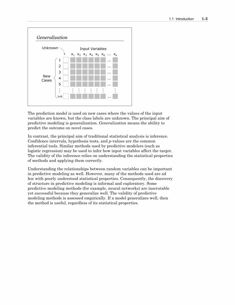
The prediction model is used on new cases where the values of the input variables are known, but the class labels are unknown. The principal aim of predictive modeling is generalization. Generalization means the ability to predict the outcome on novel cases.
In contrast, the principal aim of traditional statistical analysis is inference. Confidence intervals, hypothesis tests, and p-values are the common inferential tools. Similar methods used by predictive modelers (such as logistic regression) may be used to infer how input variables affect the target. The validity of the inference relies on understanding the statistical properties of methods and applying them correctly.
Understanding the relationships between random variables can be important in predictive modeling as well. However, many of the methods used are ad hoc with poorly understood statistical properties. Consequently, the discovery of structure in predictive modeling is informal and exploratory. Some predictive modeling methods (for example, neural networks) are inscrutable yet successful because they generalize well. The validity of predictive modeling methods is assessed empirically. If a model generalizes well, then the method is useful, regardless of its statistical properties.

1-4 Chapter 1 Predictive Modeling
Applications
• Target Marketing
• Attrition Prediction
• Credit Scoring
• Fraud Detection
There are many business applications of predictive modeling. Database marketing uses customer databases to improve sales promotions and product loyalty. In target marketing, the cases are customers, the inputs are attributes such as previous purchase history and demographics, and the target is often a binary variable indicating a response to a past promotion. The aim is to find segments of customers that are likely to respond to some offer so they can be targeted. Historic customer databases can also be used to predict who is likely to switch brands or cancel services (churn). Loyalty promotions can then be targeted at new cases that are at risk.
Credit scoring (Hand and Henley 1997) is used to decide whether to extend credit to applicants. The cases are past applicants. Most input variables come from the credit application or credit reports. A relevant binary target is whether the case defaulted (charged-off) or paid-off the debt. The aim is to reduce defaults and serious delinquencies on new applicants for credit.
In fraud detection, the cases are transactions (for example, telephone calls, credit card purchases) or insurance claims. The inputs are the particulars and circumstances of the transaction. The binary target is whether that case was fraudulent. The aim is to anticipate fraud or abuse on new transactions or claims so that they can be investigated or impeded.
Supervised classification also has less business-oriented uses. Image classification has applications in areas such as astronomy, nuclear medicine, and molecular genetics (McLachlan 1992; Ripley 1996; Hand 1997).

1.1 Introduction 1-5
Demonstration 1
The INS data set is a retail-banking example. The data set has 32,264 cases (banking customers) and 47 input variables. The binary target variable INS indicates whether the customer has an insurance product (variable annuity). The 47 input variables represent other product usage and demographics prior to their acquiring the insurance product. Two of the inputs are nominally scaled; the others are interval or binary.
The DATA step reads in the original data and creates a data set in the work library. This prevents writing over the original data.
libname read 'SAS−data−library'; data develop; set read.ins; run;
The %LET statement enables you to define a macro variable and assign it a value. The statement below creates a macro variable called INPUTS and assigns it a string that contains all the numeric input variable names. This reduces the amount of text you need to enter in other programs.
%let inputs=acctage dda ddabal dep depamt cashbk checks dirdep nsf nsfamt phone teller atm atmamt pos posamt cd cdbal ira irabal loc locbal inv invbal ils ilsbal mm mmbal mmcred mtg mtgbal sav savbal cc ccbal ccpurc sdb income hmown lores hmval age crscore moved inarea;
The MEANS procedure generates descriptive statistics for the numeric variables. The statistics requested below are the number of observations, the number of missing values, the mean, the minimum value, and the maximum value. The macro variable, INPUTS, is referenced in the VAR statement by prefixing an ampersand (&) to the macro variable name. The FREQ procedure examines the values of the target variable and the nominal input variables.
proc means data=develop n nmiss mean min max; var &inputs; run;

1-6 Chapter 1 Predictive Modeling
proc freq data=develop; tables ins branch res; run;
The MEANS Procedure
N Variable Label N Miss Mean ƒƒƒƒƒƒƒƒƒƒƒƒƒƒƒƒƒƒƒƒƒƒƒƒƒƒƒƒƒƒƒƒƒƒƒƒƒƒƒƒƒƒƒƒƒƒƒƒƒƒƒƒƒƒƒƒƒƒƒƒƒƒƒƒƒƒƒƒƒƒƒ ACCTAGE Age of Oldest Account 30194 2070 5.9086772 DDA Checking Account 32264 0 0.8156459 DDABAL Checking Balance 32264 0 2170.02 DEP Checking Deposits 32264 0 2.1346082 DEPAMT Amount Deposited 32264 0 2232.76 CASHBK Number Cash Back 32264 0 0.0159621 CHECKS Number of Checks 32264 0 4.2599182 DIRDEP Direct Deposit 32264 0 0.2955616 NSF Number Insufficient Funds 32264 0 0.0870630 NSFAMT Amount NSF 32264 0 2.2905464 PHONE Number Telephone Banking 28131 4133 0.4056024 TELLER Teller Visits 32264 0 1.3652678 SAV Saving Account 32264 0 0.4668981 SAVBAL Saving Balance 32264 0 3170.60 ATM ATM 32264 0 0.6099368 ATMAMT ATM withdrawl Amount 32264 0 1235.41 POS Number Point of Sale 28131 4133 1.0756816 POSAMT Amount Point of Sale 28131 4133 48.9261782 CD Certificate of Deposit 32264 0 0.1258368 CDBAL CD Balance 32264 0 2530.71 IRA Retirement Account 32264 0 0.0532792 IRABAL IRA Balance 32264 0 617.5704550 LOC Line of Credit 32264 0 0.0633833 LOCBAL Line of Credit Balance 32264 0 1175.22 INV Investment 28131 4133 0.0296826 INVBAL Investment Balance 28131 4133 1599.17 ILS Installment Loan 32264 0 0.0495909 ILSBAL Loan Balance 32264 0 517.5692375 MM Money Market 32264 0 0.1148959 MMBAL Money Market Balance 32264 0 1875.76 MMCRED Money Market Credits 32264 0 0.0563786 MTG Mortgage 32264 0 0.0493429 MTGBAL Mortgage Balance 32264 0 8081.74 CC Credit Card 28131 4133 0.4830969 CCBAL Credit Card Balance 28131 4133 9586.55 CCPURC Credit Card Purchaces 28131 4133 0.1541716 SDB Saftey Deposit Box 32264 0 0.1086660 INCOME Income 26482 5782 40.5889283 HMOWN Owns Home 26731 5533 0.5418802 LORES Length of Residence 26482 5782 7.0056642 HMVAL Home Value 26482 5782 110.9121290 AGE Age 25907 6357 47.9283205 CRSCORE Credit Score 31557 707 666.4935197 MOVED Recent Address Change 32264 0 0.0296305 INAREA Local Address 32264 0 0.9602963

1.1 Introduction 1-7
Variable Label Minimum Maximum ƒƒƒƒƒƒƒƒƒƒƒƒƒƒƒƒƒƒƒƒƒƒƒƒƒƒƒƒƒƒƒƒƒƒƒƒƒƒƒƒƒƒƒƒƒƒƒƒƒƒƒƒƒƒƒƒƒƒƒƒƒƒƒƒƒƒƒƒƒ ACCTAGE Age of Oldest Account 0.3000000 61.5000000 DDA Checking Account 0 1.0000000 DDABAL Checking Balance -774.8300000 278093.83 DEP Checking Deposits 0 28.0000000 DEPAMT Amount Deposited 0 484893.67 CASHBK Number Cash Back 0 4.0000000 CHECKS Number of Checks 0 49.0000000 DIRDEP Direct Deposit 0 1.0000000 NSF Number Insufficient Funds 0 1.0000000 NSFAMT Amount NSF 0 666.8500000 PHONE Number Telephone Banking 0 30.0000000 TELLER Teller Visits 0 27.0000000 SAV Saving Account 0 1.0000000 SAVBAL Saving Balance 0 700026.94 ATM ATM 0 1.0000000 ATMAMT ATM withdrawl Amount 0 427731.26 POS Number Point of Sale 0 54.0000000 POSAMT Amount Point of Sale 0 3293.49 CD Certificate of Deposit 0 1.0000000 CDBAL CD Balance 0 1053900.00 IRA Retirement Account 0 1.0000000 IRABAL IRA Balance 0 596497.60 LOC Line of Credit 0 1.0000000 LOCBAL Line of Credit Balance -613.0000000 523147.24 INV Investment 0 1.0000000 INVBAL Investment Balance -2214.92 8323796.02 ILS Installment Loan 0 1.0000000 ILSBAL Loan Balance 0 29162.79 MM Money Market 0 1.0000000 MMBAL Money Market Balance 0 120801.11 MMCRED Money Market Credits 0 5.0000000 MTG Mortgage 0 1.0000000 MTGBAL Mortgage Balance 0 10887573.28 CC Credit Card 0 1.0000000 CCBAL Credit Card Balance -2060.51 10641354.78 CCPURC Credit Card Purchases 0 5.0000000 SDB Saftey Deposit Box 0 1.0000000 INCOME Income 0 233.0000000 HMOWN Owns Home 0 1.0000000 LORES Length of Residence 0.5000000 19.5000000 HMVAL Home Value 67.0000000 754.0000000 AGE Age 16.0000000 94.0000000 CRSCORE Credit Score 509.0000000 820.0000000 MOVED Recent Address Change 0 1.0000000 INAREA Local Address 0 1.0000000
The results of PROC MEANS show that several variables have missing values and several variables are binary.

1-8 Chapter 1 Predictive Modeling
The FREQ Procedure Insurance Product Cumulative Cumulative INS Frequency Percent Frequency Percent ƒƒƒƒƒƒƒƒƒƒƒƒƒƒƒƒƒƒƒƒƒƒƒƒƒƒƒƒƒƒƒƒƒƒƒƒƒƒƒƒƒƒƒƒƒƒƒƒƒƒƒƒƒƒƒƒ 0 21089 65.36 21089 65.36 1 11175 34.64 32264 100.00 Primary Branch Cumulative Cumulative BRANCH Frequency Percent Frequency Percent ƒƒƒƒƒƒƒƒƒƒƒƒƒƒƒƒƒƒƒƒƒƒƒƒƒƒƒƒƒƒƒƒƒƒƒƒƒƒƒƒƒƒƒƒƒƒƒƒƒƒƒƒƒƒƒƒƒƒƒ B1 2819 8.74 2819 8.74 B10 273 0.85 3092 9.58 B11 247 0.77 3339 10.35 B12 549 1.70 3888 12.05 B13 535 1.66 4423 13.71 B14 1072 3.32 5495 17.03 B15 2235 6.93 7730 23.96 B16 1534 4.75 9264 28.71 B17 850 2.63 10114 31.35 B18 541 1.68 10655 33.02 B19 285 0.88 10940 33.91 B2 5345 16.57 16285 50.47 B3 2844 8.81 19129 59.29 B4 5633 17.46 24762 76.75 B5 2752 8.53 27514 85.28 B6 1438 4.46 28952 89.73 B7 1413 4.38 30365 94.11 B8 1341 4.16 31706 98.27 B9 558 1.73 32264 100.00 Area Classification Cumulative Cumulative RES Frequency Percent Frequency Percent ƒƒƒƒƒƒƒƒƒƒƒƒƒƒƒƒƒƒƒƒƒƒƒƒƒƒƒƒƒƒƒƒƒƒƒƒƒƒƒƒƒƒƒƒƒƒƒƒƒƒƒƒƒƒƒƒ R 8077 25.03 8077 25.03 S 11506 35.66 19583 60.70 U 12681 39.30 32264 100.00
The results of PROC FREQ show that 34.6 percent of the observations have acquired the insurance product. There are 19 levels of BRANCH and 3 levels under RES (R=rural, S=suburb, U=urban).

1.2 Analytical Challenges 1-9
1.2 Analytical Challenges
289765837 5828966527 8488544512987639810883873736365342987156347878976487879976542454313451561618100192879101019816176336290098754641874687815753687123169597788913251144564856 82354 58722 87989531540891974561687241672118766+651687117874354644544477545876541019834 4573829200919283645275243265127004069857 654732714171189387400383686576615456019917361342700292714519635438765 9172198000938745498738186 15435 4343831716681118451476875743355454163561654645246454681524684135413551844871354684158461683168234223o28787545287346249819617576576762927561727492 1072387107061076401 872567654716526479 675574510017564588 596176578357754965340715064045 740347634681848764464741873244586412189978769429871648000252452389019836354431417618192030305060708089685747663635242762819109385027945624183004573421317 8590583624563839938 26569218387732880347343421359849679841348198384709174910974709810971978666666616249116498619640457026461491763592076597278001801163915302039 08725009450278563987674507672895798628739898720234762762876471647467546287475464778355958875750009370387825377835668 76987260289748870 71708798616716454 431232039080560094509398349829838019801432168 561084 135482164618456 173741648 1470900109 091913132541245134154364154632020940980632457641387541254714764872765401901801887165196 79198715685 65882 7820023928276525343039837873537595987736527830900898
Opportunistic Data
• Operational/Observational
• Massive
• Errors and Outliers
• Missing Values
The data that is typically used to develop predictive models can be characterized as opportunistic. It was collected for operational purposes unrelated to statistical analysis (Huber 1997). Such data is usually massive, dynamic, and dirty. Preparing data for predictive modeling can be agonizing. For example, the parts of the data that are relevant to the analysis need to be acquired. Furthermore, the relevant inputs usually need to be created from the raw operational fields. Many statistical methods do not scale well to massive data sets because most methods were developed for small data sets generated from designed experiments.

1-10 Chapter 1 Predictive Modeling
Mixed Measurement Scales
sales, executive, homemaker, ...
88.60, 3.92, 34890.50, 45.01, ...
0, 1, 2, 3, 4, 5, 6, ...
F, D, C, B, A
27513, 21737, 92614, 10043, ...
M, F
When there are a large number of input variables, there are usually a variety of measurement scales represented. The input variable may be intervally scaled (amounts), binary, nominally scaled (names), ordinally scaled (grades), or counts. Nominal input variables with a large number of levels (such as ZIP code) are commonplace and present complications for regression analysis.

1.2 Analytical Challenges 1-11
High Dimensionality
II IIII II III III I III II
II I I III III IIII II II II
II III III I II II II II I II
X1
X2
X3
X1
X2
X1
X3
X2
X3
X1
X2
X3
The dimension refers to the number of input variables (actually input degrees of freedom). Predictive modelers consider large numbers (hundreds) of input variables. The number of variables often has a greater effect on computational performance than the number of cases. High dimensionality limits the ability to explore and model the relationships among the variables. This is known as the curse of dimensionality, which was distilled by Breiman et al. (1984) as
The complexity of a data set increases rapidly with increasing dimensionality.
The remedy is dimension reduction; ignore irrelevant and redundant dimensions without inadvertently ignoring important ones.

1-12 Chapter 1 Predictive Modeling
Rare Target Event
Eventrespondchurn
defaultfraud
No Eventnot respond
staypay off
legitimate
In predictive modeling, the event of interest is often rare. Usually more data leads to better models, but having an ever-larger number of nonevent cases has rapidly diminishing return and can even have detrimental effects. With rare events, the effective sample size for building a reliable prediction model is closer to 3× the number of event cases than to the nominal size of the data set (Harrell 1997). A seemingly massive data set might have the predictive potential of one that is much smaller.
One widespread strategy for predicting rare events is to build a model on a sample that disproportionally over-represents the event cases (for example, an equal number of events and nonevents). Such an analysis introduces biases that need to be corrected so that the results are applicable to the population.

1.2 Analytical Challenges 1-13
Nonlinearities and Interactions
LinearAdditive
NonlinearNonadditive
E(y) E(y)
x1 x2x1 x2
Predictive modeling is a multivariate problem. Each important dimension might affect the target in complicated ways. Moreover, the effect of each input variable might depend on the values of other input variables. The curse of dimensionality makes this difficult to untangle. Many classical modeling methods (including standard logistic regression) were developed for inputs with effects that have a constant rate of change and do not depend on any other inputs.
Underfitting
IIIIIIII II IIII IIIIIIIIIII
I
III IIIIIIIIIIIIIIIIIIIIIIIIIIIIIIIII
II
IIIIIIII
I
I
I
II
II
I
I
I
II
III
I
I
I
III
II
I
IIII
I
II
I
I IIII
II
IIIIIIIIIII IIIIIIIIIIII III IIIIIIIIIIII IIIIIIIIIIIIIIIIIIIIIIIIIIIIIIIIIIII
Overfitting
Just Right
Model Selection
Predictive modeling typically involves choices from among a set of models. These might be different types of models. These might be different complexities of models of the same type. A common pitfall is to overfit the data; that is, to use too complex a model. An overly complex model might be too sensitive to peculiarities in the sample data set and not generalize well to new data. Using too simple a model, however, can lead to underfitting, where true features are disregarded.

1-14 Chapter 1 Predictive Modeling
1.3 Chapter Summary
The principal objective of predictive modeling is to predict the outcome on new cases. Some of the business applications include target marketing, attrition prediction, credit scoring, and fraud detection. One challenge in building a predictive model is that the data usually was not collected for purposes of data analysis. Therefore, it is usually massive, dynamic, and dirty. For example, the data usually has a large number of input variables. This limits the ability to explore and model the relationships among the variables. Thus, detecting interactions and nonlinearities becomes a cumbersome problem.
When the target is rare, a widespread strategy is to build a model on a sample that disproportionally over-represents the events. The results will be biased, but they can be easily corrected to represent the population.
A common pitfall in building a predictive model is to overfit the data. An overfitted model will be too sensitive to the nuances in the data and will not generalize well to new data. However, a model that underfits the data will systematically miss the true features in the data.

Chapter 2 Fitting the Model
2.1 The Model ....................................................................................................................2-2
Demonstration 2..............................................................................................................2-8
Demonstration 3............................................................................................................2-14
2.2 Adjustments for Oversampling................................................................................2-16
Demonstration 4............................................................................................................2-19
Demonstration 5............................................................................................................2-24
2.3 Chapter Summary.....................................................................................................2-27

2-2 Chapter 2 Fitting the Model
2.1 The Model
Functional Form
kikii xxp β++β+β= L110)logit(
posterior probability
parameterinput
The data set consists of i=1,2,…,n cases. Each case belongs to one of two classes. A binary indicator variable represents the class label for each case
= casefor event targetno0
casefor event target1
i
iyi
Associated with each case is k-vector of input variables
( )kiiii xxx ,,, 21 K=x
The posterior probability of the target event given the inputs is
( ) ( )iiiii yyEp xx |1Pr| ===
The standard logistic regression model assumes that the logit of the posterior probability is a linear combination of the input variables. The parameters, β0,…,βk, are unknown constants that must be estimated from the data.

2.1 The Model 2-3
The Logit Link Function
η−+=⇔η=
−
=e
pp
pp i
i
ii 1
11
ln)logit(
smaller ← η → larger
pi = 1
pi = 0
A linear combination can take any value. Probability must be between zero and one. The logit transformation (which is the log of the odds) is a device for constraining the posterior probability to be between zero and one. The logit function transforms the probability scale to the real line (–∞, +∞). Therefore, modeling the logit with a linear combination gives estimated probabilities that are constrained to be between zero and one.
Logistic regression is a special case of the generalized linear model
kk xxyEg βββ +++= L110))|(( x
where the expected value of the target is linked to the linear predictor by the function g(≈). The link function depends on the scale of the target.

2-4 Chapter 2 Fitting the Model
The Fitted Surface
logit(p) p
1
0x1
x2 x1x2
0
The graph of a linear combination on the logit scale is a (hyper)plane. On the probability scale it becomes a sigmoidal surface. Different parameter values give different surfaces with different slopes and different orientations. The nonlinearity is solely due to the constrained scale of the target. The nonlinearity only appears when the fitted values are close to the limits of their sensible range (>.8 or <.2).

2.1 The Model 2-5
Interpretation
x1x2 x1
x2
Unit change in x2 ⇒
β2 change in logit
logit(p) p
100(exp(β2)-1)%change in the odds
A linear-additive model is particularly easy to interpret: each input variable affects the logit linearly. The coefficients are the slopes. Exponentiating each parameter estimate gives the odds ratios, which compares the odds of the event in one group to the odds of the event in another group. For example, the odds ratio for a binary input variable (X) would compare the odds of the event when X=1 to the odds of the event when X=0. The odds ratio represents the multiplicative effect of each input variable. Moreover, the effect of each input variable does not depend on the values of the other inputs (additivity).
However, this simple interpretation depends on the model being correctly specified. In predictive modeling, you should not presume that the true posterior probability has such a simple form. Think of the model as an approximating (hyper)plane. Consequently, you can determine the extent that the inputs are important to the approximating plane.

2-6 Chapter 2 Fitting the Model
Logistic Discrimination
0
1
x1x2
p
x1
x2
above
below
In supervised classification, the ultimate use of logistic regression is to allocate cases to classes. This is more correctly termed logistic discrimination (McClachlan 1989). An allocation rule is merely an assignment of a cutoff probability – where cases above the cutoff are allocated to class 1 and cases below the cutoff are allocated to class 0. The standard logistic discrimination model separates the classes by a linear surface ((hyper)plane). The decision boundary is always linear. Determining the best cutoff is a fundamental concern in logistic discrimination.

2.1 The Model 2-7
Maximum Likelihood Estimation
Log-l
ikel
ihoo
d
1β̂ 2β̂
The method of maximum likelihood (ML) is usually used to estimate the unknown parameters in the logistic regression model. The likelihood function is the joint probability density function of the data treated as a function of the parameters. The maximum likelihood estimates are the values of the parameters that maximize the probability of obtaining the sample data.
If you assume that the yi independently have Bernoulli distributions with probability pi (which is a function of the parameters), then the log of the likelihood is given by
( ) ∑ ∑∑= ==
−+=−−+1 0
1| 0|1
)1ln()ln()1ln()1()ln(n
yi
n
yiii
n
iiiii pppypy
where n0 and n1 are the numbers of class 0 and class 1, respectively. The form of the log-likelihood shows the intuitively appealing result that the ML estimates be chosen so that pi is large when yi=1 and small when yi=0.
In ML estimation the combination of parameter values that maximize the likelihood (or log-likelihood) are pursued. There is, in general, no closed form analytical solution for the ML estimates as there is for linear regression on a normally distributed response. They must be determined using an iterative optimization algorithm. Consequently, logistic regression is considerably more computationally expensive than linear regression.
Software for ML estimation of the logistic model is commonplace. Many SAS procedures can be used; most notable are PROC LOGISTIC, PROC GENMOD, PROC CATMOD, and PROC DMREG (Enterprise Miner).
2-8 Chapter 2 Fitting the Model
Demonstration 2
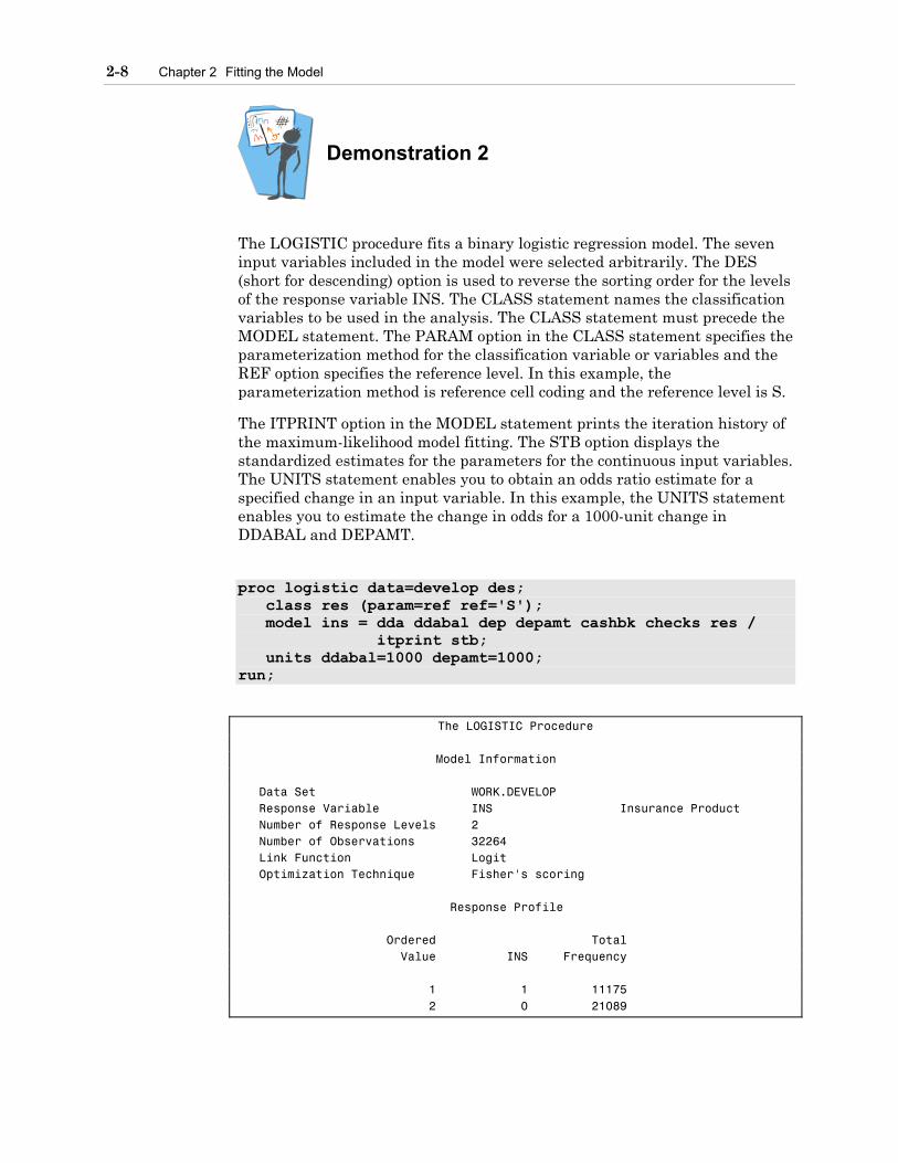
The LOGISTIC procedure fits a binary logistic regression model. The seven input variables included in the model were selected arbitrarily. The DES (short for descending) option is used to reverse the sorting order for the levels of the response variable INS. The CLASS statement names the classification variables to be used in the analysis. The CLASS statement must precede the MODEL statement. The PARAM option in the CLASS statement specifies the parameterization method for the classification variable or variables and the REF option specifies the reference level. In this example, the parameterization method is reference cell coding and the reference level is S.
The ITPRINT option in the MODEL statement prints the iteration history of the maximum-likelihood model fitting. The STB option displays the standardized estimates for the parameters for the continuous input variables. The UNITS statement enables you to obtain an odds ratio estimate for a specified change in an input variable. In this example, the UNITS statement enables you to estimate the change in odds for a 1000-unit change in DDABAL and DEPAMT.
proc logistic data=develop des; class res (param=ref ref='S'); model ins = dda ddabal dep depamt cashbk checks res / itprint stb; units ddabal=1000 depamt=1000; run;
The LOGISTIC Procedure
Model Information Data Set WORK.DEVELOP Response Variable INS Insurance Product Number of Response Levels 2 Number of Observations 32264 Link Function Logit Optimization Technique Fisher's scoring Response Profile Ordered Total Value INS Frequency 1 1 11175 2 0 21089

2.1 The Model 2-9
The results consist of a number of tables. The Response Profile table shows the target variable values listed according to their ordered values. By default, the target-variable values are ordered alphanumerically and PROC LOGISTIC always models the probability of ordered value 1. The DES option reverses the order so that PROC LOGISTIC models the probability that INS=1. Class Level Information Design Variables Class Value 1 2 RES R 1 0 S 0 0 U 0 1
The Class Level Information table shows the RES was dummy coded into 2 design variables using reference cell coding and the level S as the reference level.
Maximum Likelihood Iteration History
Iter Ridge -2 Log L Intercept DDA DDABAL 0 0 41631 -0.635072 0 0 Maximum Likelihood Iteration History Iter DEP DEPAMT CASHBK CHECKS RESR 0 0 0 0 0 0 Maximum Likelihood Iteration History Iter RESU 0 0 Maximum Likelihood Iteration History Iter Ridge -2 Log L Intercept DDA DDABAL 1 0 39713 0.207211 -0.949444 0.000036952 2 0 39555 0.151944 -0.952976 0.000063520 3 0 39547 0.151925 -0.969109 0.000071357 4 0 39547 0.151919 -0.969925 0.000071793

2-10 Chapter 2 Fitting the Model
Maximum Likelihood Iteration History
Iter DEP DEPAMT CASHBK CHECKS RESR 1 -0.068009 0.000011100 -0.432924 0.001079 -0.044160 2 -0.072362 0.000017189 -0.554889 -0.003028 -0.046869 3 -0.071516 0.000017870 -0.562999 -0.003988 -0.046718 4 -0.071448 0.000017848 -0.562921 -0.004025 -0.046712 Maximum Likelihood Iteration History Iter RESU 1 -0.036395 2 -0.038190 3 -0.037901 4 -0.037888 Last Change in -2 Log L 0.0179123969 Last Evaluation of Gradient Intercept DDA DDABAL DEP DEPAMT 0.0024101311 0.0024101295 113.21372547 0.005149575 28.376343373 Last Evaluation of Gradient CASHBK CHECKS RESR RESU 0.00003316 0.0141724821 0.0006778614 0.0008478713 Convergence criterion (GCONV=1E-8) satisfied.
The ITPRINT option produces the numeric details of the ML estimation. Four iterations were needed to fit the logistic model. At each iteration, the –2 log likelihood decreased and the parameter estimates changed.
Model Fit Statistics
Intercept Intercept and Criterion Only Covariates AIC 41633.206 39565.329 SC 41641.587 39640.765 -2 Log L 41631.206 39547.329
The Model Fit Statistics table contains the Akaike information criteria (AIC) and the Schwarz criterion (SC). These are goodness-of-fit measures you can use to compare one model to another.

2.1 The Model 2-11
Testing Global Null Hypothesis: BETA=0
Test Chi-Square DF Pr > ChiSq Likelihood Ratio 2083.8761 8 <.0001 Score 1843.2388 8 <.0001 Wald 1768.0578 8 <.0001
The likelihood ratio, Wald, and Score tests all test the null hypothesis that all regression coefficients of the model other than the intercept are 0.
Type III Analysis of Effects
Wald Effect DF Chi-Square Pr > ChiSq DDA 1 633.6092 <.0001 DDABAL 1 448.5968 <.0001 DEP 1 42.8222 <.0001 DEPAMT 1 30.6227 <.0001 CASHBK 1 24.1615 <.0001 CHECKS 1 1.6168 0.2035 RES 2 2.7655 0.2509
The Type III Analysis of Effects table shows which input variables are significant controlling for all of the other input variables in the model.
Analysis of Maximum Likelihood Estimates Standard Standardized Parameter DF Estimate Error Chi-Square Pr > ChiSq Estimate Intercept 1 0.1519 0.0304 24.8969 <.0001 DDA 1 -0.9699 0.0385 633.6092 <.0001 -0.2074 DDABAL 1 0.000072 3.39E-6 448.5968 <.0001 0.2883 DEP 1 -0.0714 0.0109 42.8222 <.0001 -0.0678 DEPAMT 1 0.000018 3.225E-6 30.6227 <.0001 0.0660 CASHBK 1 -0.5629 0.1145 24.1615 <.0001 -0.0408 CHECKS 1 -0.00402 0.00317 1.6168 0.2035 -0.0114 RES R 1 -0.0467 0.0316 2.1907 0.1388 . RES U 1 -0.0379 0.0280 1.8375 0.1752 .
The parameter estimates measure the rate of change in the logit (log odds) corresponding to a one-unit change in input variable, adjusted for the effects of the other inputs. The parameter estimates are difficult to compare because they depend on the units in which the variables are measured. The standardized estimates convert them to standard deviation units. The absolute value of the standardized estimates can be used to give an approximate ranking of the relative importance of the input variables on the fitted logistic model. The variable RES has no standardized estimate because it is a class variable.

2-12 Chapter 2 Fitting the Model
Odds Ratio Estimates Point 95% Wald Effect Estimate Confidence Limits DDA 0.379 0.352 0.409 DDABAL 1.000 1.000 1.000 DEP 0.931 0.911 0.951 DEPAMT 1.000 1.000 1.000 CASHBK 0.570 0.455 0.713 CHECKS 0.996 0.990 1.002 RES R vs S 0.954 0.897 1.015 RES U vs S 0.963 0.911 1.017
The odds ratio measures the effect of the input variable on the target adjusted for the effect of the other input variables. For example, the odds of acquiring an insurance product is .379 times less for DDA (checking account) customers than for non-DDA customers. Equivalently, the odds of acquiring an insurance product is 1/.379 or 2.64 times more likely for non-DDA customers compared to DDA customers. By default, PROC LOGISTIC reports the 95% Wald confidence interval.
Association of Predicted Probabilities and Observed Responses Percent Concordant 66.4 Somers' D 0.350 Percent Discordant 31.4 Gamma 0.358 Percent Tied 2.2 Tau-a 0.158 Pairs 235669575 c 0.675
The Association of Predicted Probabilities and Observed Responses table lists several measures that assess the predictive ability of the model. For all pairs of observations with different values of the target variable, a pair is concordant if the observation with the outcome has a higher predicted outcome probability (based on the model) than the observation without the outcome. A pair is discordant if the observation with the outcome has a lower predicted outcome probability than the observation without the outcome.
The four rank correlation indexes (Somer’s D, Gamma, Tau-a, and c) are computed from the numbers of concordant and discordant pairs of observations. In general, a model with higher values for these indexes (the maximum value is 1) has better predictive ability than a model with lower values for these indexes.
Adjusted Odds Ratios
Effect Unit Estimate DDABAL 1000.0 1.074 DEPAMT 1000.0 1.018
For continuous variables, it may be useful to convert the odds ratio to a percentage increase or decrease in odds. For example, the odds ratio for a 1000-unit change in DDABAL is 1.074. Consequently, the odds of acquiring the insurance product increases 7.4% (calculated as 100(1.074−1)) for every thousand dollar increase in the checking balance, assuming the other variables do not change.

2.1 The Model 2-13
Scoring New Cases
05.ˆ =p
)0.3,1.1(=x
21 50.14.6.1)ˆ(logit xxp +−=
The overriding purpose of predictive modeling is to score new cases. Predictions can be made by simply plugging in the new values of the inputs.

2-14 Chapter 2 Fitting the Model
Demonstration 3
The LOGISTIC procedure outputs the final parameter estimates to a data set using the OUTEST= option.
proc logistic data=develop des outest=betas1; model ins=dda ddabal dep depamt cashbk checks; run; proc print data=betas1; run;
Obs _LINK_ _TYPE_ _STATUS_ _NAME_ Intercept DDA DDABAL 1 LOGIT PARMS 0 Converged INS 0.12592 -0.97052 .000071819 Obs DEP DEPAMT CASHBK CHECKS _LNLIKE_ 1 -0.071531 .000017829 -0.56175 -.003999236 -19775.05
The output data set contains one observation and a variable for each parameter estimate. The estimates are named corresponding to their input variable.
The SCORE procedure multiplies values from two SAS data sets, one containing coefficients (SCORE=) and the other containing the data to be scored (DATA=). The data set to be scored typically would not have a target variable. The OUT= option specifies the name of the scored data set created by PROC SCORE. The TYPE=PARMS option is required for scoring regression models.
proc score data=read.new out=scored score=betas1 type=parms; var dda ddabal dep depamt cashbk checks; run;
The linear combination produced by PROC SCORE (the variable INS) estimates the logit, not the posterior probability. The logistic function (inverse of the logit) needs to be applied to compute the posterior probability.
data scored; set scored; P=1/(1+exp(-ins)); run;

2.1 The Model 2-15
proc print data=scored(obs=20); var p ins dda ddabal dep depamt cashbk checks; run;
Obs p INS DDA DDABAL DEP DEPAMT CASHBK CHECKS 1 0.27476 -0.97058 1 56.29 2 955.51 0 1 2 0.32343 -0.73807 1 3292.17 2 961.60 0 1 3 0.30275 -0.83426 1 1723.86 2 2108.65 0 2 4 0.53144 0.12592 0 0.00 0 0.00 0 0 5 0.27180 -0.98552 1 67.91 2 519.24 0 3 6 0.32482 -0.73172 1 2554.58 1 501.36 0 2 7 0.27205 -0.98425 1 0.00 2 2883.08 0 12 8 0.30558 -0.82087 1 2641.33 3 4521.61 0 8 9 0.53144 0.12592 0 0.00 0 0.00 0 0 10 0.28679 -0.91103 1 52.22 1 75.59 0 0 11 0.37131 -0.52659 1 6163.29 2 2603.56 0 7 12 0.18001 -1.51631 1 431.12 2 568.43 1 2 13 0.53144 0.12592 0 0.00 0 0.00 0 0 14 0.20217 -1.37280 1 112.82 8 2688.75 0 3 15 0.31330 -0.78473 1 1146.61 3 11224.20 0 2 16 0.53144 0.12592 0 0.00 0 0.00 0 0 17 0.27549 -0.96694 1 1241.38 3 3538.14 0 15 18 0.30509 -0.82318 1 298.23 0 0.00 0 0 19 0.28299 -0.92966 1 367.04 2 4242.22 0 11 20 0.26508 -1.01975 1 1229.47 4 3514.57 0 10
Data can also be scored directly in PROC LOGISTIC using the OUTPUT statement. This has several disadvantages over using PROC SCORE: it does not scale well with large data sets, it requires a target variable (or some proxy), and the adjustments for oversampling, discussed in a later section, are not automatically applied.

2-16 Chapter 2 Fitting the Model
2.2 Adjustments for Oversampling
(x,y),(x,y),(x,y),(x,y),(x,y),(x,y),(x,y),(x,y),(x,y),(x,y),(x,y),...
Sampling Designs
{(x,y),(x,y),(x,y),(x,y)}
x,x,x,x,x,x,x,x,x,x,x,...
y = 0 y = 1
{(x,0),(x,0),(x,1),(x,1)}x,x,x,x,x,x,x,x,x,x,x,...
Joint
Separate
In joint (mixture) sampling, the input-target pairs are randomly selected from their joint distribution. In separate sampling, the inputs are randomly selected from their distributions within each target class.
Separate sampling is standard practice in supervised classification. When the target event is rare, it is common to oversample the rare event, that is, take a disproportionately large number of event cases. Oversampling rare events is generally believed to lead to better predictions (Scott and Wild 1986). Separate sampling is also known as • case-control sampling • choice-based sampling • stratified sampling on the target, not necessarily taken with proportional
allocation • biased sampling • y-conditional sampling • outcome-dependent sampling • oversampling.
The priors, π0 and π1, represent the population proportions of class 0 and 1, respectively. The proportions of the target classes in the sample are denoted ρ0 and ρ1. In separate sampling (non-proportional) π0 ≠ ρ0 and π1 ≠ ρ1. The adjustments for oversampling require the priors be known a priori.

2.2 Adjustments for Oversampling 2-17
The Effect of Oversampling
Biased Correctedlogit
p
The maximum likelihood estimates were derived under the assumption that yi have independent Bernoulli distributions. This assumption is appropriate for joint sampling but not for separate sampling. However, the effects of violating this assumption can be easily corrected. In logistic regression, only the estimate of the intercept, β0, is affected by using Bernoulli ML on data from a separate sampling design (Prentice and Pike 1979). If the standard model
kki xxp β++β+β= L110)(logit
is appropriate for joint sampling, then ML estimates of the parameters under separate sampling can be determined by fitting the pseudo model (Scott and Wild 1986, 1997)
kki xxp βββπρπρ
++++
= L110
10
01* ln)(logit
where p* is the posterior probability corresponding to the biased sample. Consequently, the effect of oversampling is to shift the logits by a constant amount – the offset
πρπρ
10
01ln
When rare events have been oversampled π0 > ρ0 and π1 < ρ1, the offset is positive; that is, the logit is too large. This vertical shift of the logit affects the posterior probability in a corresponding fashion.
2-18 Chapter 2 Fitting the Model
Offset
01
10lnρπρπ
logit
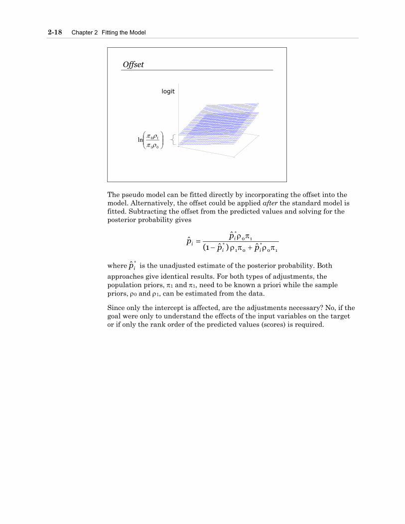
The pseudo model can be fitted directly by incorporating the offset into the model. Alternatively, the offset could be applied after the standard model is fitted. Subtracting the offset from the predicted values and solving for the posterior probability gives
10*
01*
10*
ˆ)ˆ1(
ˆˆ
πρ+πρ−πρ
=ii
ii pp
pp
where *ˆip is the unadjusted estimate of the posterior probability. Both
approaches give identical results. For both types of adjustments, the population priors, π1 and π1, need to be known a priori while the sample priors, ρ0 and ρ1, can be estimated from the data.
Since only the intercept is affected, are the adjustments necessary? No, if the goal were only to understand the effects of the input variables on the target or if only the rank order of the predicted values (scores) is required.
2.2 Adjustments for Oversampling 2-19
Demonstration 4
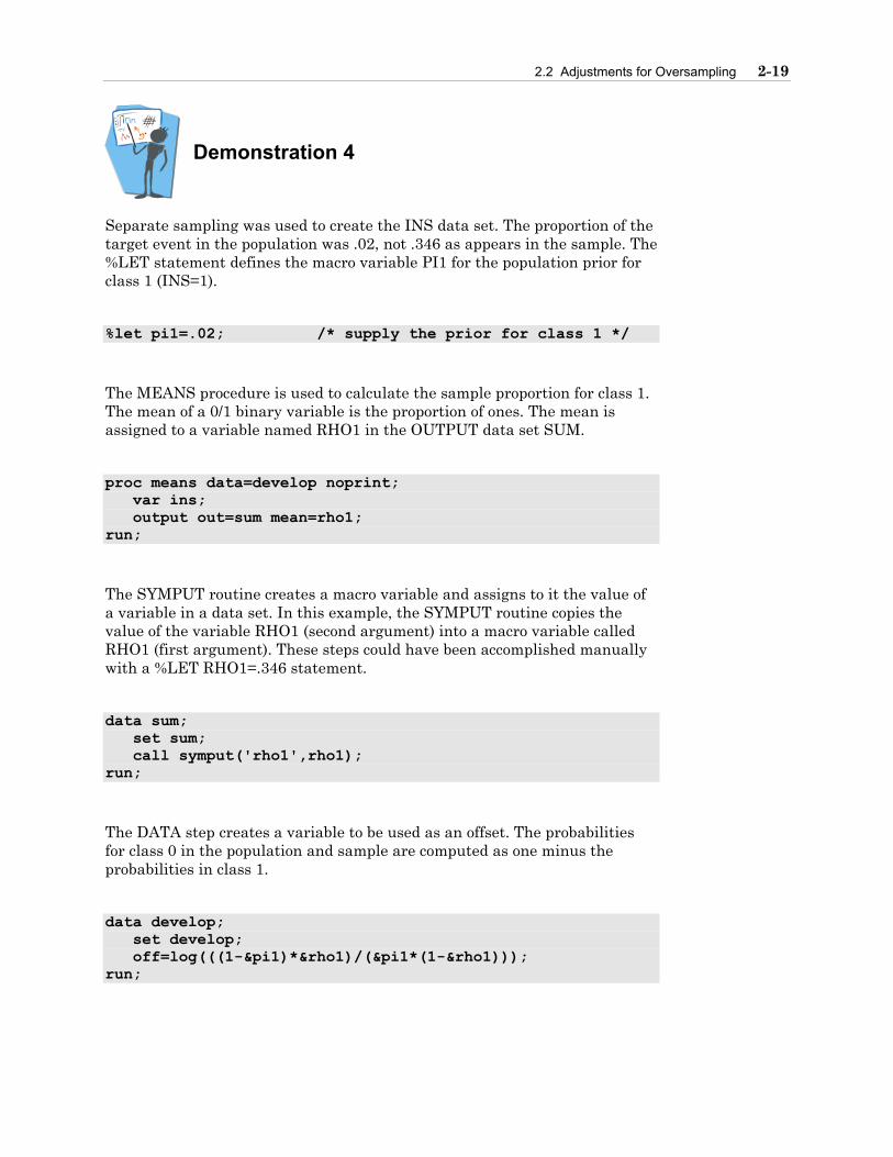
Separate sampling was used to create the INS data set. The proportion of the target event in the population was .02, not .346 as appears in the sample. The %LET statement defines the macro variable PI1 for the population prior for class 1 (INS=1).
%let pi1=.02; /* supply the prior for class 1 */
The MEANS procedure is used to calculate the sample proportion for class 1. The mean of a 0/1 binary variable is the proportion of ones. The mean is assigned to a variable named RHO1 in the OUTPUT data set SUM.
proc means data=develop noprint; var ins; output out=sum mean=rho1; run;
The SYMPUT routine creates a macro variable and assigns to it the value of a variable in a data set. In this example, the SYMPUT routine copies the value of the variable RHO1 (second argument) into a macro variable called RHO1 (first argument). These steps could have been accomplished manually with a %LET RHO1=.346 statement.
data sum; set sum; call symput('rho1',rho1); run;
The DATA step creates a variable to be used as an offset. The probabilities for class 0 in the population and sample are computed as one minus the probabilities in class 1.
data develop; set develop; off=log(((1-&pi1)*&rho1)/(&pi1*(1-&rho1))); run;

2-20 Chapter 2 Fitting the Model
The LOGISTIC procedure fits a model with the offset variable and outputs the final parameter estimates. The OFFSET= option in the MODEL statement names the offset variable. The only difference between the parameter estimates with and without the offset variable is the intercept term.
proc logistic data=develop des outest=betas2; model ins=dda ddabal dep depamt cashbk checks / offset=off; run;
Partial Output Analysis of Maximum Likelihood Estimates
Standard Parameter DF Estimate Error Chi-Square Pr > ChiSq Intercept 1 -3.1308 0.0260 14518.0451 <.0001 DDA 1 -0.9705 0.0385 634.4513 <.0001 DDABAL 1 0.000072 3.39E-6 448.8938 <.0001 DEP 1 -0.0715 0.0109 42.9169 <.0001 DEPAMT 1 0.000018 3.223E-6 30.5992 <.0001 CASHBK 1 -0.5617 0.1145 24.0544 <.0001 CHECKS 1 -0.00400 0.00317 1.5964 0.2064 off 1 1.0000 0 . .
The list of parameter estimates contains a new entry for the variable OFF, which has a fixed value of one. The probabilities computed from this model have been adjusted down because the population probability is much lower than the sample probability (.02 versus .346).
The SCORE procedure uses the final parameter estimates from the logistic model with the offset variable to score new data.
proc score data=read.new out=scored score=betas2 type=parms; var dda ddabal dep depamt cashbk checks; run; data scored; set scored; p=1/(1+exp(-ins)); run; proc print data=scored(obs=20); var p ins dda ddabal dep depamt cashbk checks; run;

2.2 Adjustments for Oversampling 2-21
Obs p INS DDA DDABAL DEP DEPAMT CASHBK CHECKS 1 0.014381 -4.22733 1 56.29 2 955.51 0 1 2 0.018078 -3.99482 1 3292.17 2 961.60 0 1 3 0.016447 -4.09101 1 1723.86 2 2108.65 0 2 4 0.041854 -3.13083 0 0.00 0 0.00 0 0 5 0.014171 -4.24227 1 67.91 2 519.24 0 3 6 0.018191 -3.98847 1 2554.58 1 501.36 0 2 7 0.014189 -4.24100 1 0.00 2 2883.08 0 12 8 0.016665 -4.07762 1 2641.33 3 4521.61 0 8 9 0.041854 -3.13083 0 0.00 0 0.00 0 0 10 0.015250 -4.16778 1 52.22 1 75.59 0 0 11 0.022241 -3.78334 1 6163.29 2 2603.56 0 7 12 0.008384 -4.77306 1 431.12 2 568.43 1 2 13 0.041854 -3.13083 0 0.00 0 0.00 0 0 14 0.009665 -4.62955 1 112.82 8 2688.75 0 3 15 0.017268 -4.04148 1 1146.61 3 11224.20 0 2 16 0.041854 -3.13083 0 0.00 0 0.00 0 0 17 0.014433 -4.22369 1 1241.38 3 3538.14 0 15 18 0.016628 -4.07993 1 298.23 0 0.00 0 0 19 0.014973 -4.18641 1 367.04 2 4242.22 0 11 20 0.013701 -4.27650 1 1229.47 4 3514.57 0 10
The OFFSET= option is less efficient than fitting an unadjusted model. When the OFFSET= option is used, PROC LOGISTIC uses CPU time roughly equivalent to two logistic regressions. A more efficient way of adjusting the posterior probabilities for the offset is to fit the model without the offset and adjust the fitted posterior probabilities afterwards in a DATA step. The two approaches are statistically equivalent.
proc logistic data=develop des outest=betas3; model ins=dda ddabal dep depamt cashbk checks; run; proc score data=read.new out=scored score=betas3 type=parms; var dda ddabal dep depamt cashbk checks; run; data scored; set scored; off=log(((1-&pi1)*&rho1)/(&pi1*(1-&rho1))); p=1/(1+exp(-(ins-off))); run; proc print data=scored(obs=20); var p ins dda ddabal dep depamt cashbk checks; run;
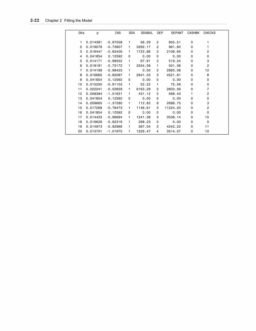
2-22 Chapter 2 Fitting the Model
Obs p INS DDA DDABAL DEP DEPAMT CASHBK CHECKS 1 0.014381 -0.97058 1 56.29 2 955.51 0 1 2 0.018078 -0.73807 1 3292.17 2 961.60 0 1 3 0.016447 -0.83426 1 1723.86 2 2108.65 0 2 4 0.041854 0.12592 0 0.00 0 0.00 0 0 5 0.014171 -0.98552 1 67.91 2 519.24 0 3 6 0.018191 -0.73172 1 2554.58 1 501.36 0 2 7 0.014189 -0.98425 1 0.00 2 2883.08 0 12 8 0.016665 -0.82087 1 2641.33 3 4521.61 0 8 9 0.041854 0.12592 0 0.00 0 0.00 0 0 10 0.015250 -0.91103 1 52.22 1 75.59 0 0 11 0.022241 -0.52659 1 6163.29 2 2603.56 0 7 12 0.008384 -1.51631 1 431.12 2 568.43 1 2 13 0.041854 0.12592 0 0.00 0 0.00 0 0 14 0.009665 -1.37280 1 112.82 8 2688.75 0 3 15 0.017268 -0.78473 1 1146.61 3 11224.20 0 2 16 0.041854 0.12592 0 0.00 0 0.00 0 0 17 0.014433 -0.96694 1 1241.38 3 3538.14 0 15 18 0.016628 -0.82318 1 298.23 0 0.00 0 0 19 0.014973 -0.92966 1 367.04 2 4242.22 0 11 20 0.013701 -1.01975 1 1229.47 4 3514.57 0 10
2.2 Adjustments for Oversampling 2-23
Sampling Weights
=ρπ
=ρπ
=0if
1if
0
0
1
1
i
i
i
y
yweight
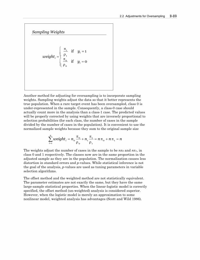
Another method for adjusting for oversampling is to incorporate sampling weights. Sampling weights adjust the data so that it better represents the true population. When a rare target event has been oversampled, class 0 is under-represented in the sample. Consequently, a class-0 case should actually count more in the analysis than a class-1 case. The predicted values will be properly corrected by using weights that are inversely proportional to selection probabilities (for each class, the number of cases in the sample divided by the number of cases in the population). It is convenient to use the normalized sample weights because they sum to the original sample size
nnnnnweightn
ii =π+π=
ρπ
+ρπ
=∑=
101
11
0
00
1
The weights adjust the number of cases in the sample to be nπ0 and nπ1, in class 0 and 1 respectively. The classes now are in the same proportion in the adjusted sample as they are in the population. The normalization causes less distortion in standard errors and p-values. While statistical inference is not the goal of the analysis, p-values are used as tuning parameters in variable selection algorithms.
The offset method and the weighted method are not statistically equivalent. The parameter estimates are not exactly the same, but they have the same large-sample statistical properties. When the linear-logistic model is correctly specified, the offset method (un-weighted) analysis is considered superior. However, when the logistic model is merely an approximation to some nonlinear model, weighted analysis has advantages (Scott and Wild 1986).

2-24 Chapter 2 Fitting the Model
Demonstration 5
The DATA step adds the sampling weights to the data set DEVELOP. The weights are .058 (.02/.346) for class 1 and 1.5 (.98/.654) for class 0. They could have been assigned manually without having to reference macro variables. The logical expressions (INS=1) and (INS=0) in the assignment statement return the value one when true and zero when false. Consequently, this syntax is a more compact way of expressing a conditional.
/* The variable INS is the target variable */ data develop; set develop; sampwt=((1-&pi1)/(1-&rho1))*(ins=0) +(&pi1/&rho1)*(ins=1); run;
The WEIGHT statement in PROC LOGISTIC weights each observation in the input data set by the value of the WEIGHT variable.
proc logistic data=develop des outest=betas4; weight sampwt; model ins = dda ddabal dep depamt cashbk checks/stb; run;
The LOGISTIC Procedure
Model Information Data Set WORK.DEVELOP Response Variable INS Insurance Product Number of Response Levels 2 Number of Observations 32264 Weight Variable sampwt Sum of Weights 32263.999999 Link Function Logit Optimization Technique Fisher's scoring Response Profile Ordered Total Total Value INS Frequency Weight 1 1 11175 645.280 2 0 21089 31618.720
2.2 Adjustments for Oversampling 2-25
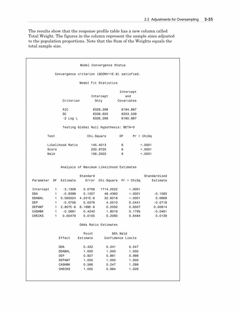
The results show that the response profile table has a new column called Total Weight. The figures in the column represent the sample sizes adjusted to the population proportions. Note that the Sum of the Weights equals the total sample size.
Model Convergence Status
Convergence criterion (GCONV=1E-8) satisfied. Model Fit Statistics Intercept Intercept and Criterion Only Covariates AIC 6328.268 6194.867 SC 6336.650 6253.539 -2 Log L 6326.268 6180.867 Testing Global Null Hypothesis: BETA=0 Test Chi-Square DF Pr > ChiSq Likelihood Ratio 145.4013 6 <.0001 Score 230.9720 6 <.0001 Wald 156.2503 6 <.0001 Analysis of Maximum Likelihood Estimates Standard Standardized Parameter DF Estimate Error Chi-Square Pr > ChiSq Estimate Intercept 1 -3.1308 0.0756 1714.2522 <.0001 DDA 1 -0.8398 0.1207 48.4360 <.0001 -0.1583 DDABAL 1 0.000024 4.241E-6 32.6018 <.0001 0.0669 DEP 1 -0.0756 0.0376 4.0510 0.0441 -0.0718 DEPAMT 1 2.807E-6 6.199E-6 0.2050 0.6507 0.00814 CASHBK 1 -0.5691 0.4240 1.8016 0.1795 -0.0461 CHECKS 1 0.00479 0.0105 0.2080 0.6484 0.0139 Odds Ratio Estimates Point 95% Wald Effect Estimate Confidence Limits DDA 0.432 0.341 0.547 DDABAL 1.000 1.000 1.000 DEP 0.927 0.861 0.998 DEPAMT 1.000 1.000 1.000 CASHBK 0.566 0.247 1.299 CHECKS 1.005 0.984 1.026

2-26 Chapter 2 Fitting the Model
Association of Predicted Probabilities and Observed Responses
Percent Concordant 53.6 Somers' D 0.282 Percent Discordant 25.3 Gamma 0.358 Percent Tied 21.1 Tau-a 0.128 Pairs 235669575 c 0.641
The parameter estimates are similar but not equivalent to those from the pseudo model. The weighted analysis also changed the goodness-of-fit measures, the standardized estimates, and the rank correlation indexes. These statistics are not correct when using the WEIGHT statement and should be interpreted with caution.
proc score data=read.new out=scored score=betas4 type=parms; var dda ddabal dep depamt cashbk checks; run; data scored; set scored; p=1/(1+exp(-ins)); run; proc print data=scored(obs=20); var p ins dda ddabal dep depamt cashbk checks; run;
Obs p INS DDA DDABAL DEP DEPAMT CASHBK CHECKS 1 0.016095 -4.11301 1 56.29 2 955.51 0 1 2 0.017385 -4.03463 1 3292.17 2 961.60 0 1 3 0.016880 -4.06460 1 1723.86 2 2108.65 0 2 4 0.041854 -3.13083 0 0.00 0 0.00 0 0 5 0.016233 -4.10437 1 67.91 2 519.24 0 3 6 0.018463 -3.97338 1 2554.58 1 501.36 0 2 7 0.017019 -4.05625 1 0.00 2 2883.08 0 12 8 0.016586 -4.08248 1 2641.33 3 4521.61 0 8 9 0.041854 -3.13083 0 0.00 0 0.00 0 0 10 0.017213 -4.04475 1 52.22 1 75.59 0 0 11 0.019232 -3.93175 1 6163.29 2 2603.56 0 7 12 0.009292 -4.66930 1 431.12 2 568.43 1 2 13 0.041854 -3.13083 0 0.00 0 0.00 0 0 14 0.010447 -4.55090 1 112.82 8 2688.75 0 3 15 0.015850 -4.12861 1 1146.61 3 11224.20 0 2 16 0.041854 -3.13083 0 0.00 0 0.00 0 0 17 0.016535 -4.08560 1 1241.38 3 3538.14 0 15 18 0.018644 -3.96338 1 298.23 0 0.00 0 0 19 0.017152 -4.04834 1 367.04 2 4242.22 0 11 20 0.014986 -4.18553 1 1229.47 4 3514.57 0 10 The probabilities from the weighted analysis are similar but not equivalent to the probabilities estimated by the offset method (pseudo model).

2.3 Chapter Summary 2-27
2.3 Chapter Summary
The standard logistic regression model assumes that the logit of the posterior probability is a linear combination of the input variables. The logit transformation is used to constrain the posterior probability to be between zero and one. The parameter estimates are estimated using the method of maximum likelihood. This method finds the parameter estimates that are most likely to occur given the data. When you exponentiate the slope estimates, you obtain the odds ratio which compares the odds of the event in one group to the odds of the event in another group.
An efficient way to score new cases is to output the final parameter estimates from PROC LOGISTIC and then use PROC SCORE to compute the predicted logits for each case. A DATA step can then be used to take the inverse of the logit to compute the posterior probability.
When you oversample rare events, you can use the OFFSET option to adjust the model so that the posterior probabilities reflect the population. You can also use the WEIGHT statement to adjust the data so that the posterior probabilities reflect the population. The two methods are not statistically equivalent. When the linear-logistic model is correctly specified, the offset method is considered superior. However, when the logistic model is merely an approximation to some nonlinear model, the weighted analysis has advantages.
General form of PROC LOGISTIC:
PROC LOGISTIC DATA=SAS-data-set <options>; CLASS variables </option>; WEIGHT variable; MODEL response=predictors </options>; UNITS predictor1=list1 </option>; RUN;
General form of PROC SCORE:
PROC SCORE DATA=SAS-data-set <options>; VAR variables; RUN;

2-28 Chapter 2 Fitting the Model

Chapter 3 Preparing the Input Variables
3.1 Missing Values ............................................................................................................3-2
Demonstration 6..............................................................................................................3-6
3.2 Categorical Inputs.....................................................................................................3-10
Demonstration 7............................................................................................................3-14
3.3 Variable Clustering ...................................................................................................3-21
Demonstration 8............................................................................................................3-27
3.4 Subset Selection.......................................................................................................3-36
Demonstration 9............................................................................................................3-37
Demonstration 10..........................................................................................................3-47
3.5 Chapter Summary.....................................................................................................3-52

3-2 Chapter 3 Preparing the Input Variables
3.1 Missing Values
Does Pr(missing) Depend on the Data?
14
67
?
33
18
6
31
51
2
1
3
1
2
0
3
1
2
4
1
7
1
1
8
8
• No
–MCAR
• Yes
– that unobserved value
–other observed values
–other unobserved values
Missing values of the input variables can arise from several different mechanisms (Little 1992). A value is missing completely at random (MCAR) if the probability that it is missing is independent of the data. MCAR is a particularly easy mechanism to manage but is unrealistic in most predictive modeling applications.
The probability that a value is missing might depend on the unobserved value – credit applicants with fewer years at their current job might be less inclined to provide this information.
The probability that a value is missing might depend on observed values of other input variables – customers with longer tenures might be less likely to have certain historic transactional data. Missingness might depend on a combination of values of correlated inputs.
An even more pathological missing-value mechanism occurs when the probability that a value is missing depends on values of unobserved (lurking) predictors – transient customers might have missing values on a number of variables.
A fundamental concern for predictive modeling is that the missingness is related to the target – maybe the more transient customers are the best prospects for a new offer.

3.1 Missing Values 3-3
Complete Case AnalysisCas
esInput Variables
The default method for treating missing values in most SAS modeling procedures (including the LOGISTIC procedure) is complete case analysis. In complete-case analysis, only those cases without any missing values are used in the analysis.
Complete-case analysis has some moderately attractive theoretical properties even when the missingness depends on observed values of other inputs (Donner 1982; Jones 1996). However, complete-case analysis has serious practical shortcomings with regards to predictive modeling. Even a smattering of missing values can cause an enormous loss of data in high dimensions. For instance, suppose each of the k input variables can be MCAR with probability α; in this situation, the expected proportion of complete cases is
( )kα−1
Therefore, a 1% probability of missing (α=.01) for 100 inputs would leave only 37% of the data for analysis, 200 would leave 13%, and 400 would leave 2%. If the missingness was increased to 5% (α=.05), then <1% of the data would be available with 100 inputs.

3-4 Chapter 3 Preparing the Input Variables
New Missing Values
321 4.189.072.1.2)ˆlogit( xxxp −−+−=
Fitted Model:
New Case: ( ) ( )5.?,,2,, 321 −=xxx
7.)(89.144.1.2)ˆlogit( +−+−=p
Predicted Value:
Another practical consideration of any treatment of missing values is scorability (the practicality of method when it is deployed). The purpose of predictive modeling is scoring new cases. How would a model built on the complete cases score a new case if it had a missing value? To decline to score new incomplete cases would only be practical if there were a very small number of missings.
Missing Value Imputation
6.5 2.3 .33 66
C99
01
0.8 0 C99
6.5 63
12 04 1.8 0 0.5 86 65 C14
01 4.8 37 C00
8 01 2.1 1 4.8 37 64 C08
6 01 2.8 1 9.6 22 66
3 2.7 0 1.1 28 64 C00
2 02 2.1 1 5.9 21 63 C03
10 03 2.0 0 63
7 01 2.5 0 5.5 62 67 C12
01 2.4 0 0.9 29 C05
6 03 2.6 0 8.3 42 66 C03
Because of the aforementioned drawbacks of complete-case analysis, some type of missing value imputation is necessary. Imputation means filling in the missing values with some reasonable value. Many methods have been developed for imputing missing values (Little 1992). The principal consideration for most methods is getting valid statistical inference on the imputed data, not generalization.
Often, subject-matter knowledge can be used to impute missing data. For example, the missing values might be miscoded zeros.

3.1 Missing Values 3-5
3463.22265418.4720
Median = 30
34633022265418304920
0010000100
CompletedData
MissingIndicator
IncompleteData
Imputation + Indicators
One reasonable strategy for handling missing values in predictive modeling is to
1. Create missing indicators
=otherwise0
missing is if1 jj
xMI
and treat them as new input variables in the analysis.
2. Use median imputation – fill the missing value of xj with the median of the complete cases for that variable.
3. Create a new level representing missing (unknown) for categorical inputs.
If a very large percentage of values are missing (>50%), then the variable might be better handled by omitting it from the analysis or by creating the missing indicator only. If a very small percentage of the values are missing (<1%), then the missing indicator is of little value.
This strategy is somewhat unsophisticated but satisfies two of the most important considerations in predictive modeling: scorability and the potential relationship of missingness with the target. A new case is easily scored; first replace the missing values with the medians from the development data and then apply the prediction model.
There is statistical literature concerning different missing value imputation methods, including discussions of the demerits of mean and median imputation and missing indicators (Donner 1982; Jones 1997). Unfortunately, most of the advice is based on considerations that are peripheral to predictive modeling. There is very little advice when the functional form of the model is not assumed to be correct, when the goal is to get good predictions that can be practically applied to new cases, when p-values and hypothesis tests are largely irrelevant, and when the missingness may be highly pathological – depending on lurking predictors.

3-6 Chapter 3 Preparing the Input Variables
Demonstration 6
The objective of the following program is to create missing value indicator variables and to replace missing values with the variable median.
proc print data=develop(obs=30); var ccbal ccpurc income hmown; run;
Obs CCBAL CCPURC INCOME HMOWN 1 483.65 0 16 1 2 0.00 1 4 1 3 0.00 0 30 1 4 65.76 0 125 1 5 0.00 0 25 1 6 38.62 0 19 0 7 85202.99 0 55 1 8 0.00 0 13 0 9 . . 20 0 10 0.00 0 54 0 11 0.00 0 . . 12 0.00 0 25 1 13 . . 102 1 14 . . 24 1 15 0.00 0 8 1 16 0.00 0 100 1 17 323.13 0 13 1 18 . . 17 0 19 . . 8 1 20 0.00 0 7 1 21 0.00 0 . . 22 32366.86 0 . 1 23 0.00 0 9 0 24 . . 45 1 25 . . 36 1 26 1378.46 1 60 1 27 . . 35 1 28 17135.95 0 40 1 29 0.00 0 42 0 30 0.00 0 112 1

3.1 Missing Values 3-7
Fifteen of the input variables were selected for imputation. Two arrays are created, one called MI, which contains the missing value indicator variables, and one called X, which contains the input variables. It is critical that the order of the variables in the array MI matches the order of the variables in array X. Defining the dimension with an asterisk causes the array elements to be automatically counted. In the DO loop, the DIM function returns the dimension of the array. Thus, the DO loop will execute 15 times in this example. The assignment statement inside the DO loop causes the entries of MI to be 1 if the corresponding entry in X is missing, and zero otherwise.
data develop1; set develop; /* name the missing indicator variables */ array mi{*} miacctag miphone mipos miposamt miinv miinvbal micc miccbal miccpurc miincome mihmown milores mihmval miage micrscor; /* select variables with missing values */ array x{*} acctage phone pos posamt inv invbal cc ccbal ccpurc income hmown lores hmval age crscore; do i=1 to dim(mi); mi{i}=(x{i}=.); end; run;
The STDIZE procedure with the REPONLY option can be used to replace missing values. The METHOD= option allows you to choose several different location measures such as the mean, median, and midrange. The output data set created by the OUT= option contains all the variables in the input data set where the variables listed in the VAR statement are imputed. Only numeric input variables should be used in PROC STDIZE.
proc stdize data=develop1 reponly method=median out=imputed; var &inputs; run; proc print data=imputed(obs=20); var ccbal miccbal ccpurc miccpurc income miincome hmown mihmown; run;
PROC STANDARD with the REPLACE option can be used to replace missing values with the mean of that variable on the non-missing cases.

3-8 Chapter 3 Preparing the Input Variables
Obs CCBAL miccbal CCPURC miccpurc INCOME miincome HMOWN mihmown 1 483.65 0 0 0 16 0 1 0 2 0.00 0 1 0 4 0 1 0 3 0.00 0 0 0 30 0 1 0 4 65.76 0 0 0 125 0 1 0 5 0.00 0 0 0 25 0 1 0 6 38.62 0 0 0 19 0 0 0 7 85202.99 0 0 0 55 0 1 0 8 0.00 0 0 0 13 0 0 0 9 0.00 1 0 1 20 0 0 0 10 0.00 0 0 0 54 0 0 0 11 0.00 0 0 0 35 1 1 1 12 0.00 0 0 0 25 0 1 0 13 0.00 1 0 1 102 0 1 0 14 0.00 1 0 1 24 0 1 0 15 0.00 0 0 0 8 0 1 0 16 0.00 0 0 0 100 0 1 0 17 323.13 0 0 0 13 0 1 0 18 0.00 1 0 1 17 0 0 0 19 0.00 1 0 1 8 0 1 0 20 0.00 0 0 0 7 0 1 0

3.1 Missing Values 3-9
Cluster Imputation
X1 =
X2 = ?
Mean-imputation uses the unconditional mean of the variable. An attractive extension would be to use the mean conditional on the other inputs. This is referred to as regression imputation. Regression imputation would usually give better estimates of the missing values. Specifically, k linear regression models could be built – one for each input variable using the other inputs as predictors. This would presumably give better imputations and be able to accommodate missingness that depends on the values of the other inputs. An added complication is that the other inputs may have missing values. Consequently, the k imputation regressions also need to accommodate missing values.
Cluster-mean imputation is a somewhat more practical alternative:
1. cluster the cases into relatively homogenous subgroups
2. mean-imputation within each group
3. for new cases with multiple missing values, use the cluster mean that is closest in all the nonmissing dimensions.
This method can accommodate missingness that depends on the other input variables. This method is implemented in the Enterprise Miner.
A simple but less effective alternative is to define a priori segments (for example, high, middle, low, and unknown income), and then do mean or median imputation within each segment (Exercise 2).

3-10 Chapter 3 Preparing the Input Variables
3.2 Categorical Inputs
Dummy Variables
000011001...
010000000...
001100010...
100000100...
DA DB DC DDDBCCAADCA...
X
With the CLASS statement, you can use categorical input variables in the LOGISTIC procedure without having to create dummy variables in a DATA step. You can specify the type of parameterization to use, such as effect coding and reference coding, and the reference level. The choice of the reference level is immaterial in predictive modeling because different reference levels give the same predictions.
Smarter Variables
7510015015015075100150100...
111011101...
121133213...
HomeVal Local
998019962299523995239973799937995339952399622
...
Zip ...Urbanicity
Expanding categorical inputs into dummy variables can greatly increase the dimension of the input space. A “smarter” method is to use subject-matter information to create new inputs that represent relevant sources of variation. A categorical input might be best thought of as a link to other data sets. For example, geographic areas are often mapped to several relevant demographic variables.

3.2 Categorical Inputs 3-11
Quasi-Complete Separation
28
16
94
23
7
0
11
21
A
B
C
D
0 1
1
0
0
0
0
1
0
0
0
0
1
0
DA DB Dc
0
0
0
1
DD
Including categorical inputs in the model can cause quasi-complete separation. Quasi-complete separation occurs when a level of the categorical input has a target event rate of 0 or 100%. The coefficient of a dummy variable represents the difference in the logits between that level and the reference level. When quasi-complete separation occurs, one of the logits will be infinite, the likelihood does not have a maximum in at least one dimension, so the ML estimate of that coefficient will be infinite. If the zero-cell category is the reference level, then all the coefficients for the dummy variables will be infinite.
Quasi-complete separation complicates model interpretation. It can also affect the convergence of the estimation algorithm. Furthermore, it might lead to incorrect decisions regarding variable selection.
The most common cause of quasi-complete separation in predictive modeling is categorical inputs with rare categories. The best remedy for sparseness is collapsing levels of the categorical variable.

3-12 Chapter 3 Preparing the Input Variables
Clustering Levels
χ2 =
B & C A & BC ABC & D
A
B
C
D
0 1
28
110
23
7
11
21
138
23
18
21161 39
28
16
94
23
7
0
11
21
31.7 30.7 28.6 0
Merged:
0 10 1
0 1
100% 97% 90% 0%
Ideally, subject-matter considerations should be used to collapse levels (reduce the dimension) of categorical inputs. This is not always practical in predictive modeling. A simple data-driven method for collapsing levels of contingency tables was developed by Greenacre (1988, 1993). The levels (rows) are hierarchically clustered based on the reduction in the chi-squared test of association between the categorical variable and the target. At each step, the two levels that give the least reduction in the chi-squared statistic are merged. The process is continued until the reduction in chi-squared drops below some threshold (for example, 99%). This method will quickly throw rare categories in with other categories that have similar marginal response rates. While this method is simple and effective, there is a potential loss of information because only univariate associations are considered.

3.2 Categorical Inputs 3-13
Output Delivery System
SAS procedure computes
results
Output object
created in ODS
ODS converts data component into SAS data set
The Output Delivery System (ODS) is used in the method to collapse levels in contingency tables. This system enables you to take output from a SAS procedure and convert it to a SAS data set. Instead of writing to the listing file directly. SAS procedures can now create an output object for each piece of output that is displayed. For example, each table produced in the CLUSTER procedure is now a separate entity in the system. You can then take the data component of the output object and convert it to a SAS data set. This means that every number in every table of every procedure can be accessed via a data set.
ODS Statements
• LISTINGopens, manages, or closes the Listing destination
• TRACEprovides information about the output object such as the name and path
• OUTPUTcreates SAS data set from an output object.
The LISTING statement is used to manage the SAS listing destination. The TRACE statement is used to obtain the name of the output object. The OUTPUT statement is used to create a SAS data set.

3-14 Chapter 3 Preparing the Input Variables
Demonstration 7
The levels of a categorical input can be clustered using Greenacre’s method (1988, 1993) in PROC CLUSTER. PROC CLUSTER was designed for general clustering applications, but with some simple pre-processing of the data, it can be made to cluster levels of categorical variables.
The variable BRANCH has 19 levels. The first step is to create a data set that contains the proportion of the target event (INS) and number of cases in each level. The NWAY option caused the OUTPUT data set to have 19 observations, one for each of the 19 levels. The OUTPUT data set also has a variable PROP for the proportion of target events. It automatically creates the variable _FREQ_, which counts the number of cases in each level.
proc means data=imputed noprint nway; class branch; var ins; output out=levels mean=prop; run; proc print data=levels; run;
Obs BRANCH _TYPE_ _FREQ_ prop
1 B1 1 2819 0.36999 2 B10 1 273 0.40293 3 B11 1 247 0.35628 4 B12 1 549 0.36430 5 B13 1 535 0.37196 6 B14 1 1072 0.19123 7 B15 1 2235 0.24251 8 B16 1 1534 0.27771 9 B17 1 850 0.37059 10 B18 1 541 0.35675 11 B19 1 285 0.38596 12 B2 1 5345 0.32460 13 B3 1 2844 0.38186 14 B4 1 5633 0.37493 15 B5 1 2752 0.38118 16 B6 1 1438 0.37830 17 B7 1 1413 0.34678 18 B8 1 1341 0.38553 19 B9 1 558 0.37814
Using the FREQ statement and the METHOD=WARD in PROC CLUSTER gives identical results to Greenacre’s method. The OUTTREE= option creates an output data set that can be used by the TREE procedure to draw a tree diagram. The ID statement specifies a variable that identifies observations in

3.2 Categorical Inputs 3-15
the printed cluster history and in the OUTTREE= data set. The ODS TRACE statement with the LISTING option will show which output objects are associated with each table in the PROC CLUSTER output.
ods trace on/listing; proc cluster data=levels method=ward outtree=fortree; freq _freq_; var prop; id branch; run; ods trace off;
The CLUSTER Procedure Ward's Minimum Variance Cluster Analysis Output Added: ------------- Name: EigenvalueTable Label: Eigenvalues of the Covariance Matrix Template: stat.cluster.EigenvalueTable Path: Cluster.EigenvalueTable ------------- Eigenvalues of the Covariance Matrix Eigenvalue Difference Proportion Cumulative 1 0.00245716 1.0000 1.0000 Root-Mean-Square Total-Sample Standard Deviation = 0.04957 Root-Mean-Square Distance Between Observations = 0.070102 Output Added: ------------- Name: ClusterHistory Label: Cluster History Template: stat.cluster.ClusterHistory Path: Cluster.ClusterHistory -------------

3-16 Chapter 3 Preparing the Input Variables
Cluster History T i NCL -------Clusters Joined-------- FREQ SPRSQ RSQ e 18 B6 B9 1996 0.0000 1.00 17 B11 B18 788 0.0000 1.00 16 B19 B8 1626 0.0000 1.00 15 B1 B17 3669 0.0000 1.00 14 B3 B5 5596 0.0000 1.00 13 CL15 B13 4204 0.0000 1.00 12 CL14 CL18 7592 0.0002 1.00 11 CL13 B12 4753 0.0002 1.00 10 CL16 CL12 9218 0.0004 .999 9 CL17 B7 2201 0.0006 .999 8 CL11 B4 10386 0.0009 .998 7 B10 CL10 9491 0.0015 .996 6 CL8 CL7 19877 0.0058 .990 5 CL9 B2 7546 0.0130 .977 4 B15 B16 3769 0.0142 .963 3 B14 CL4 4841 0.0453 .918 2 CL6 CL5 27423 0.1399 .778 1 CL2 CL3 32264 0.7779 .000 The column labeled RSQ in the output is equivalent to the proportion of chi-squared in the 19×2 contingency table remaining after the levels are collapsed. At each step, the levels that give the smallest decrease in chi-squared are merged. The change in chi-squared is listed in the SPRSQ column. The rows in the summary represent the results after the listed clusters were merged. The number of clusters is reduced from 18 to 1. When previously collapsed levels are merged, they are denoted using the CL as the prefix and the number of resulting clusters as the suffix. For example, at the sixth step CL15 represents B1 and B17 that were merged at the fourth step creating 15 clusters.
To calculate the optimum number of clusters, the chi-square statistic and the associated p-value needs to be computed for each collapsed contingency table. This information can be obtained by multiplying the chi-square statistic from the 19x2 contingency table with the proportion of chi-squared remaining after the levels are collapsed. Therefore, the next program converts the output object CLUSTERHISTORY to an output data set. The FREQ procedure is used to compute the chi-square statistic for the 19x2 contingency table.
ods listing close; ods output clusterhistory=cluster; proc cluster data=levels method=ward; freq _freq_; var prop; id branch; run; ods listing;

3.2 Categorical Inputs 3-17
proc print data=cluster; run; Number FreqOf Of New Semipartial Obs Clusters Idj1 Idj2 Cluster RSq RSquared Tie 1 18 B6 B9 1996 0.0000 1.00 2 17 B11 B18 788 0.0000 1.00 3 16 B19 B8 1626 0.0000 1.00 4 15 B1 B17 3669 0.0000 1.00 5 14 B3 B5 5596 0.0000 1.00 6 13 CL15 B13 4204 0.0000 1.00 7 12 CL14 CL18 7592 0.0002 1.00 8 11 CL13 B12 4753 0.0002 1.00 9 10 CL16 CL12 9218 0.0004 .999 10 9 CL17 B7 2201 0.0006 .999 11 8 CL11 B4 10386 0.0009 .998 12 7 B10 CL10 9491 0.0015 .996 13 6 CL8 CL7 19877 0.0058 .990 14 5 CL9 B2 7546 0.0130 .977 15 4 B15 B16 3769 0.0142 .963 16 3 B14 CL4 4841 0.0453 .918 17 2 CL6 CL5 27423 0.1399 .778 18 1 CL2 CL3 32264 0.7779 .000 proc freq data=imputed noprint; tables branch*ins / chisq; output out=chi(keep=_pchi_) chisq; run; proc print data=chi; run;
Obs _PCHI_ 1 350.164
The DATA step computes the chi-square statistic for each collapsed contingency table. The _n_ variable is used to put the overall chi-square value in each observation for the data set CUTOFF. The function LOGSDF computes the log of the probability that an observation from a specified distribution is greater than or equal to a specified value. The arguments for the function are the specified distribution in quotes, the numeric random variable, and the degrees of freedom. The log of the p-value is calculated in order to produce a more visually appealing graph. data cutoff; if _n_ = 1 then set chi; set cluster; chisquare=_pchi_*rsquared; degfree=numberofclusters-1; logpvalue=logsdf('CHISQ',chisquare,degfree); run;

3-18 Chapter 3 Preparing the Input Variables
The PLOT procedure plots the log of the p-value by the number of clusters. The VPOS option specifies the number of print positions on the vertical axis. proc plot data=cutoff; plot logpvalue*numberofclusters/vpos=30; run;
The graph shows that the 4, 5, and 6 cluster solutions had the lowest p-values.
To find the cluster solution with the lowest p-value, use the MINID option in the MEANS procedure. This option finds the value of NUMBEROFCLUSTERS associated with the minimum value of LOGPVALUE and assigns that value to the variable NCL. The CALL SYMPUT routine is used to create a macro variable NCL. proc means data=cutoff noprint; var logpvalue; output out=small minid(logpvalue(numberofclusters))=ncl; run; data small; set small; call symput('ncl',ncl); run;

3.2 Categorical Inputs 3-19
The TREE procedure produces a high resolution dendrogram. The H= option specifies the variable to be used as the height axis of the dendrogram. In this example, the proportion of the chi-squared statistic is the vertical axis. proc tree data=fortree nclusters=&ncl out=clus h=rsq; id branch; run;
The dendrogram shows that several branches can be combined with a miniscule reduction in chi-squared. The horizontal axis is also roughly ordered by the mean proportion of events in each cluster. Choosing a cluster near the center of the tree (for example, B11, B18, B7, and B2) as a reference group may lead to better models if the variable selection method you choose incrementally adds variables to the model (Cohen 1991). The OUT= data set from PROC TREE shows which levels of BRANCH are associated with each cluster (provided the NCLUSTERS= option is correctly specified).
proc sort data=clus; by clusname; run; proc print data=clus; by clusname; id clusname; run;

3-20 Chapter 3 Preparing the Input Variables
CLUSNAME BRANCH CLUSTER B14 B14 5 B15 B15 3 B16 B16 4 CL5 B11 2 B18 2 B7 2 B2 2 CL6 B6 1 B9 1 B19 1 B8 1 B1 1 B17 1 B3 1 B5 1 B13 1 B12 1 B4 1 B10 1
A DATA step is used to assign the branches to dummy variables. Four dummy variables are created with the second cluster designated as the reference level. Note that the dummy variables are numbered sequentially.
data imputed; set imputed; brclus1=(branch in ('B6','B9','B19','B8','B1','B17', 'B3','B5','B13','B12','B4','B10')); brclus2=(branch='B15'); brclus3=(branch='B16'); brclus4=(branch='B14'); run;

3.3 Variable Clustering 3-21
3.3 Variable Clustering
Redundancy
x3
x5
x1
x3
x5
x1
Including redundant inputs can degrade the analysis by • destabilizing the parameter estimates • increasing the risk of overfitting • confounding interpretation • increasing computation time • increasing scoring effort • increasing the cost of data collection and augmentation.
Redundancy is an unsupervised concept – it does not involve the target variable. In contrast, irrelevant inputs are not substantially related to the target. In high dimensional data sets, identifying irrelevant inputs is more difficult than identifying redundant inputs. A good strategy is to first reduce redundancy and then tackle irrelevancy in a lower dimension space.

3-22 Chapter 3 Preparing the Input Variables
Principal Components
1 –.11 –.03 –.69 –.04
1 –.14 .07 .04
1 .04 –.73
1 .02
1
X1 X2 X3 X4 X5
1.8 0 0 0 0
1.7 0 0 0
1.0 0 0
0.3 0
0.3
PC1 PC2 PC3 PC4 PC5
CorrelationMatrix
CovarianceMatrix
Principal components analysis (Jackson 1991) can be used for reducing redundant dimensions. A set of k variables can be transformed into a set of k principal components. The principal components (PCs) are linear combinations of the k variables constructed to be jointly uncorrelated and to explain the total variability among the original (standardized) variables.
The correlation matrix is the covariance matrix of the standardized variables. Since each standardized variable has a variance equal to one, the total variability among the standardized variables is just the number of variables. The principal components are produced by an eigen-decomposition of the correlation matrix. The eigenvalues are the variances of the PCs; they sum to the number of variables. The first PC corresponds to the first eigenvalue and explains the largest proportion of the variability. Each PC explains a decreasing amount of the total variability. In the above example, the first three PCs explain 90% of the total variability.
In practice, dimension reduction is achieved by retaining only the first few PCs provided they explain a sufficient proportion of the total variation. The reduced set of PCs might then be used in place of the original variables in the analysis.

3.3 Variable Clustering 3-23
Cluster Components
1 –.11 –.03 –.69 –.04
1 –.14 .07 .04
1 .04 –.73
1 .02
1
X1 X2 X3 X4 X5
1 –.01 –.10
1 –.09
1
Clus1 Clus2 Clus3
CorrelationMatrix
CovarianceMatrix
Variable clustering as implemented in the VARCLUS procedure (SAS Institute Inc. 1990) is an alternative method for eliminating redundant dimensions that is closely related to principal components analysis. The result of clustering k variables is a set of ≤ k cluster components. Like PCs, the cluster components are linear combinations of the original variables. Unlike the PCs, the cluster components are not uncorrelated and do not explain all the variability in the original variables. The cluster components (scores) are standardized to have unit variance.
The three cluster components in the above example correspond to eigenvalues of 1.7, 1.7, and 1.0. Consequently, 88% of variation among the original (standardized) variables is explained by the three clusters.

3-24 Chapter 3 Preparing the Input Variables
Coefficients
x1
x2
x3
x4
x5
–.28
.22
–.63
.26
.64
–.64
.08
.31
.65
–.63
.09
.97
.04
–.14
–.20
.70
.03
–.09
.70
–.08
.12
.11
.70
.04
.69
0
0
.54
0
–.37
.56
0
0
–.39
0
0
1
0
0
0
Clus1 Clus2 Clus3PC1 PC2 PC3 PC4 PC5
The chief advantage of variable clustering over principal components is the coefficients. The coefficients of the PCs (eigenvectors) are usually nonzero for all the original variables. Thus, even if only a few PCs were used, all the inputs would still have to be retained in the analysis. In contrast, the cluster component scores have nonzero coefficients on disjoint subsets of the variables. These subsets correspond to disjoint clusters of the original variables. In the above example, the clusters are {x3, x5}, {x1, x4}, and {x2}.

3.3 Variable Clustering 3-25
Divisive Clustering
{X1, X2, X3, X4, X5}
{X2, X3, X5}
{X1, X4}{X3, X5}
{X1}{X2} {X4}{X3} {X5}
2nd Eigenvalue
1.7
1
.7
0
Variable clustering finds groups of variables that are as correlated as possible among themselves and as uncorrelated as possible with variables in other clusters. The basic algorithm is binary and divisive – all variables start in one cluster. A principal components analysis is done on the variables in the cluster. If the second eigenvalue is greater than a specified threshold (in other words, there is more than one dominant dimension), then the cluster is split. The PC scores are then rotated obliquely so that the variables can be split into two groups. This process is repeated for the two child clusters until the second eigenvalue drops below the threshold. (By default, PROC VARCLUS does a non-hierarchical version of this algorithm where variables can also be reassigned to other clusters.)
Larger thresholds for the second eigenvalue give fewer clusters and less of the variation is explained. Smaller thresholds give more clusters and more of the variation is explained. The value 1 is a common choice for the threshold because it represents the average size of the eigenvalues. To account for sampling variability, smaller values such as .7 have been suggested (Jackson 1991).

3-26 Chapter 3 Preparing the Input Variables
Cluster Representatives
2closestnext
2clusterown 2
11ratio 1
RRR
−−
=−
↓⇒↑↓
⇒↓−↑−
11
As with principal components analysis, dimension reduction could be achieved by replacing the original variables with the cluster scores (components). A simple alternative is to select a representative variable from each cluster. An ideal representative would have high correlation with its own cluster and have a low correlation with the other clusters. Consequently, variables with the lowest 1– R2 ratio (defined above) in each cluster would be good representatives. Of course, subject-matter considerations might dictate the selection of other representatives.

3.3 Variable Clustering 3-27
Demonstration 8
The VARCLUS procedure clusters numeric variables. The MAXEIGEN= option specifies the largest permissible value of the second eigenvalue in each cluster. The default is 1 (using the correlation matrix). The SHORT option suppresses some of the output. The OUTREE= option creates an output data set that can be used in the TREE procedure. When the OUTREE= option is used, the clusters at different levels maintain a hierarchical structure that prevents variables from transferring from one cluster to another after the split is made. If the OUTREE= option is not used, then use the HI option to get a hierarchical structure. The VAR statement lists the numeric variables to cluster: the original numeric inputs, the missing indicators, and the dummy variables for the collapsed BRANCH (64 total).
ods trace on/listing; proc varclus data=imputed maxeigen=.7 outtree=fortree short; var &inputs brclus1-brclus4 miacctag miphone mipos miposamt miinv miinvbal micc miccbal miccpurc miincome mihmown milores mihmval miage micrscor; run; ods trace off;
Partial Output Output Added: ------------- Name: ClusterSummary Label: Cluster Summary Template: Stat.Varclus.ClusterSummary Path: Varclus.GROUP.ClusterSummary ------------- Cluster summary for 1 cluster Cluster Variation Proportion Second Cluster Members Variation Explained Explained Eigenvalue ƒƒƒƒƒƒƒƒƒƒƒƒƒƒƒƒƒƒƒƒƒƒƒƒƒƒƒƒƒƒƒƒƒƒƒƒƒƒƒƒƒƒƒƒƒƒƒƒƒƒƒƒƒƒƒƒƒƒƒƒƒƒƒƒƒƒƒƒƒƒƒƒ 1 64 64 9.228833 0.1442 5.0980 Total variation explained = 9.228833 Proportion = 0.1442 Cluster 1 will be split. Output Added: ------------- Name: ConvergenceStatus Label: Convergence Status Template: Stat.Varclus.ConvergenceStatus Path: Varclus.GROUP.ConvergenceStatus -------------

3-28 Chapter 3 Preparing the Input Variables
Oblique Principal Component Cluster Analysis Clustering algorithm converged. Output Added: ------------- Name: ClusterSummary Label: Cluster Summary Template: Stat.Varclus.ClusterSummary Path: Varclus.GROUP.ClusterSummary ------------- Cluster summary for 2 clusters Cluster Variation Proportion Second Cluster Members Variation Explained Explained Eigenvalue ƒƒƒƒƒƒƒƒƒƒƒƒƒƒƒƒƒƒƒƒƒƒƒƒƒƒƒƒƒƒƒƒƒƒƒƒƒƒƒƒƒƒƒƒƒƒƒƒƒƒƒƒƒƒƒƒƒƒƒƒƒƒƒƒƒƒƒƒƒƒƒƒ 1 44 44 9.197308 0.2090 3.1689 2 20 20 5.047314 0.2524 2.0602 Total variation explained = 14.24462 Proportion = 0.2226 Output Added: ------------- Name: RSquare Label: R-squared Template: Stat.Varclus.RSquare Path: Varclus.GROUP.RSquare ------------- R-squared with ƒƒƒƒƒƒƒƒƒƒƒƒƒƒƒƒ Own Next 1-R**2 Variable Cluster Variable Cluster Closest Ratio Label ƒƒƒƒƒƒƒƒƒƒƒƒƒƒƒƒƒƒƒƒƒƒƒƒƒƒƒƒƒƒƒƒƒƒƒƒƒƒƒƒƒƒƒƒƒƒƒƒƒƒƒƒƒƒƒƒƒƒƒƒƒƒƒƒƒƒƒƒƒƒƒƒƒ Cluster 1 ACCTAGE 0.0004 0.0002 0.9998 Age of Oldest Account DEP 0.0010 0.0001 0.9991 Checking Deposits DEPAMT 0.0007 0.0000 0.9993 Amount Deposited CASHBK 0.0003 0.0000 0.9997 Number Cash Back CHECKS 0.0037 0.0001 0.9964 Number of Checks NSF 0.0002 0.0001 0.9999 Number Insufficient Funds PHONE 0.0180 0.0001 0.9821 Number Telephone Banking TELLER 0.0012 0.0001 0.9989 Teller Visits SAV 0.0006 0.0000 0.9994 Saving Account ATM 0.0003 0.0000 0.9997 ATM ATMAMT 0.0013 0.0000 0.9987 ATM withdrawl Amount POS 0.0258 0.0000 0.9743 Number Point of Sale POSAMT 0.0242 0.0001 0.9758 Amount Point of Sale CD 0.0002 0.0000 0.9998 Certificate of Deposit CDBAL 0.0002 0.0000 0.9998 CD Balance LOC 0.0066 0.0000 0.9934 Line of Credit LOCBAL 0.0014 0.0001 0.9987 Line of Credit Balance INV 0.0052 0.0001 0.9949 Investment INVBAL 0.0002 0.0000 0.9999 Investment Balance ILS 0.0026 0.0000 0.9975 Installment Loan ILSBAL 0.0024 0.0000 0.9977 Loan Balance MMBAL 0.0000 0.0000 1.0000 Money Market Balance MTG 0.0032 0.0002 0.9970 Mortgage MTGBAL 0.0006 0.0000 0.9995 Mortgage Balance CC 0.1279 0.0007 0.8727 Credit Card

3.3 Variable Clustering 3-29
R-squared with ƒƒƒƒƒƒƒƒƒƒƒƒƒƒƒƒ Own Next 1-R**2 Variable Cluster Variable Cluster Closest Ratio Label ƒƒƒƒƒƒƒƒƒƒƒƒƒƒƒƒƒƒƒƒƒƒƒƒƒƒƒƒƒƒƒƒƒƒƒƒƒƒƒƒƒƒƒƒƒƒƒƒƒƒƒƒƒƒƒƒƒƒƒƒƒƒƒƒƒƒƒƒƒƒƒƒƒ CCBAL 0.0019 0.0000 0.9981 Credit Card Balance CCPURC 0.0212 0.0000 0.9788 Credit Card Purchaces SDB 0.0006 0.0000 0.9995 Saftey Deposit Box CRSCORE 0.0001 0.0000 0.9999 Credit Score MOVED 0.0000 0.0000 1.0000 Recent Address Change INAREA 0.0002 0.0000 0.9998 Local Address brclus1 0.2238 0.0535 0.8200 brclus2 0.5331 0.0022 0.4679 brclus3 0.0061 0.0019 0.9958 brclus4 0.2426 0.0010 0.7582 miacctag 0.0000 0.0000 1.0000 miphone 0.9924 0.0044 0.0076 mipos 0.9924 0.0044 0.0076 miposamt 0.9924 0.0044 0.0076 miinv 0.9924 0.0044 0.0076 miinvbal 0.9924 0.0044 0.0076 micc 0.9924 0.0044 0.0076 miccbal 0.9924 0.0044 0.0076 miccpurc 0.9924 0.0044 0.0076 ------------------------------------------------------------------------- Cluster 2 DDA 0.0002 0.0001 0.9999 Checking Account DDABAL 0.0004 0.0001 0.9997 Checking Balance DIRDEP 0.0001 0.0001 1.0000 Direct Deposit NSFAMT 0.0000 0.0000 1.0000 Amount NSF SAVBAL 0.0000 0.0000 1.0000 Saving Balance IRA 0.0000 0.0000 1.0000 Retirement Account IRABAL 0.0001 0.0000 0.9999 IRA Balance MM 0.0000 0.0000 1.0000 Money Market MMCRED 0.0000 0.0000 1.0000 Money Market Credits INCOME 0.0114 0.0000 0.9887 Income HMOWN 0.1850 0.0000 0.8150 Owns Home LORES 0.0005 0.0001 0.9996 Length of Residence HMVAL 0.0138 0.0000 0.9863 Home Value AGE 0.0009 0.0000 0.9991 miincome 0.9857 0.0028 0.0144 mihmown 0.9540 0.0030 0.0461 milores 0.9857 0.0028 0.0144 mihmval 0.9857 0.0028 0.0144 miage 0.9194 0.0027 0.0808 micrscor 0.0044 0.0000 0.9956 Cluster 1 will be split. The output from PROC VARCLUS shows the results for each step in the divisive clustering algorithm. Even with the SHORT option, the amount of printed output is voluminous. However, with the output delivery system, you can just print the results of the last step of the algorithm. The output object RSQUARE contains the results of each iteration of the algorithm except the first one (the cluster with all of the variables). To print out the last iteration, you need the number of clusters in the last iteration.

3-30 Chapter 3 Preparing the Input Variables
Partial Output (continued) Output Added: ------------- Name: ClusterQuality Label: Cluster Quality Template: Stat.Varclus.ClusterQuality Path: Varclus.ClusterQuality ------------- Total Proportion Minimum Maximum Minimum Number Variation of Variation Proportion Second R-squared of Explained Explained Explained Eigenvalue for a Clusters by Clusters by Clusters by a Cluster in a Cluster Variable ƒƒƒƒƒƒƒƒƒƒƒƒƒƒƒƒƒƒƒƒƒƒƒƒƒƒƒƒƒƒƒƒƒƒƒƒƒƒƒƒƒƒƒƒƒƒƒƒƒƒƒƒƒƒƒƒƒƒƒƒƒƒƒƒƒƒƒƒƒƒƒƒƒƒ 1 9.228833 0.1442 0.1442 5.097981 0.0000 2 14.244622 0.2226 0.2090 3.168931 0.0000 3 17.326324 0.2707 0.1131 2.580865 0.0000 4 19.816263 0.3096 0.1743 2.060186 0.0000 5 21.818048 0.3409 0.1445 1.944758 0.0000 6 23.714281 0.3705 0.1445 1.799784 0.0000 7 25.493053 0.3983 0.1743 1.608465 0.0000 8 26.922505 0.4207 0.2237 1.510815 0.0000 9 28.422066 0.4441 0.2581 1.315813 0.0000 10 29.720976 0.4644 0.2581 1.301067 0.0000 11 30.965926 0.4838 0.2581 1.277914 0.0004 12 32.233788 0.5037 0.2778 1.275369 0.0004 13 33.417658 0.5222 0.2778 1.202271 0.0004 14 34.478793 0.5387 0.2778 1.176730 0.0004 15 35.616145 0.5565 0.2778 1.122456 0.0004 16 36.735160 0.5740 0.2778 1.047389 0.0004 17 37.512875 0.5861 0.2778 1.014122 0.0004 18 38.499809 0.6016 0.2778 1.014092 0.0004 19 39.510304 0.6173 0.2778 1.006026 0.0004 20 40.516326 0.6331 0.3634 1.000278 0.0029 21 41.509294 0.6486 0.3634 0.999117 0.0029 22 42.508387 0.6642 0.3634 0.998695 0.0037 23 43.507082 0.6798 0.3634 0.998156 0.0037 24 44.505237 0.6954 0.3634 0.993723 0.0495 25 45.498960 0.7109 0.3634 0.992708 0.0495 26 46.485792 0.7263 0.3634 0.985980 0.0495 27 47.471431 0.7417 0.3634 0.979783 0.1052 28 48.412387 0.7564 0.3634 0.975309 0.1885 29 49.195234 0.7687 0.3634 0.946039 0.1885 30 50.085015 0.7826 0.5257 0.911070 0.1885 31 50.996084 0.7968 0.5257 0.889327 0.1885 32 51.885412 0.8107 0.5257 0.885500 0.1885 33 52.768506 0.8245 0.5257 0.844004 0.1885 34 53.611665 0.8377 0.5257 0.839114 0.2281 35 54.450779 0.8508 0.5257 0.824195 0.2281 36 55.272149 0.8636 0.6271 0.793655 0.2281 37 56.064721 0.8760 0.6271 0.745734 0.4055 38 56.810455 0.8877 0.6322 0.735552 0.4055 39 57.546007 0.8992 0.6414 0.732613 0.4055 40 58.274506 0.9105 0.6414 0.692052 0.4865

3.3 Variable Clustering 3-31
Oblique Principal Component Cluster Analysis Maximum Number 1-R**2 Ratio of for a Clusters Variable ƒƒƒƒƒƒƒƒƒƒƒƒƒƒƒƒƒƒƒƒƒ 1 2 1.0000 3 1.3758 4 1.3879 5 1.2892 6 1.2892 7 1.9744 8 1.9658 9 1.7101 10 1.7101 11 1.7101 12 1.9257 13 1.9257 14 1.9257 15 2.7382 16 2.7382 17 2.7382 18 2.7382 19 1.4776 20 1.4776 21 1.4776 22 1.4776 23 1.4776 24 1.4776 25 1.4776 26 1.4776 27 1.4776 28 1.4776 29 1.4776 30 1.4776 31 1.4776 32 2.3045 33 2.3045 34 2.3045 35 2.3045 36 2.3045 37 2.3045 38 2.3045 39 2.3045 40 2.3045
The variable NUMBEROFCLUSTERS in the output object CLUSTERQUALITY contains the number of clusters for the final iteration. The output object also has information on the proportion of variation explained by the clusters and the maximum second eigenvalue in a cluster. This information can be used to decide whether too few or too many clusters have been formed.

3-32 Chapter 3 Preparing the Input Variables
The ODS OUTPUT statement creates a SAS data set called SUMMARY from the output object CLUSTERQUALITY. The MATCH_ALL option instructs ODS to create a separate data set for each RSQUARE object that is created at each iteration. The first data set is called CLUSTERS, the second data set is called CLUSTERS1, and so on. Since the total number of clusters in the final iteration is 40, and since the first iteration does not have a RSQUARE object, the last data set is called CLUSTERS38.
The call SYMPUT routine creates the macro variable NCL, which contains the value of the number of clusters in the last iteration of the clustering algorithm minus 2. The TRIM and LEFT functions are used to eliminate the leading blanks.
By combining the macro variable NCL with the text ‘CLUSTERS’, the PRINT procedure prints the last iteration of the divisive clustering algorithm. The data set that is printed out is CLUSTERS38.
ods listing close; ods output clusterquality=summary rsquare(match_all)=clusters; proc varclus data=imputed maxeigen=.7 short hi; var &inputs brclus1-brclus4 miacctag miphone mipos miposamt miinv miinvbal micc miccbal miccpurc miincome mihmown milores mihmval miage micrscor; run; ods listing; data _null_; set summary; call symput('ncl',trim(left(numberofclusters-2))); run; proc print data=clusters&ncl; run;

3.3 Variable Clustering 3-33
V R a N S r C O e q i o w x u a n V n t a b t C a C C r l r l r l l e e o u i u o R L l s a s s a a O V t b t e t b b a e l e s i e s r r e r t o l 1 Cluster 1 brclus2 0.5684 0.1194 0.4901 2 miphone 0.9962 0.2339 0.0050 3 mipos 0.9962 0.2339 0.0050 4 miposamt 0.9962 0.2339 0.0050 5 miinv 0.9962 0.2339 0.0050 6 miinvbal 0.9962 0.2339 0.0050 7 micc 0.9962 0.2339 0.0050 8 miccbal 0.9962 0.2339 0.0050 9 miccpurc 0.9962 0.2339 0.0050 10 - Cluster 2 miincome 0.9936 0.1336 0.0074 11 mihmown 0.9624 0.1266 0.0431 12 milores 0.9936 0.1336 0.0074 13 mihmval 0.9936 0.1336 0.0074 14 miage 0.9255 0.1047 0.0832 15 - Cluster 3 DEP 0.7236 0.3197 0.4063 Checking Deposits 16 CHECKS 0.7139 0.1951 0.3554 Number of Checks 17 TELLER 0.4865 0.0456 0.5380 Teller Visits 18 - Cluster 4 MTGBAL 0.9687 0.1976 0.0390 Mortgage Balance 19 CCBAL 0.9687 0.1333 0.0361 Credit Card Balance 20 - Cluster 5 INCOME 0.8419 0.0268 0.1625 Income 21 HMVAL 0.8419 0.3218 0.2332 Home Value 22 - Cluster 6 ILS 0.9958 0.0380 0.0044 Installment Loan 23 ILSBAL 0.9958 0.0380 0.0044 Loan Balance 24 - Cluster 7 MM 0.7722 0.9011 2.3045 Money Market 25 MMCRED 0.7722 0.2705 0.3123 Money Market Credits 26 - Cluster 8 POS 0.9189 0.0711 0.0873 Number Point of Sale 27 POSAMT 0.9189 0.0622 0.0864 Amount Point of Sale 28 - Cluster 9 CD 0.7252 0.0161 0.2793 Certificate of Deposit 29 CDBAL 0.7252 0.0263 0.2823 CD Balance 30 - Cluster 10 LOC 0.7352 0.0336 0.2740 Line of Credit 31 LOCBAL 0.7352 0.0632 0.2827 Line of Credit Balance 32 - Cluster 11 CC 0.6872 0.1065 0.3501 Credit Card 33 CCPURC 0.6872 0.0538 0.3306 Credit Card Purchases 34 - Cluster 12 IRA 0.6732 0.0459 0.3426 Retirement Account 35 IRABAL 0.6732 0.0217 0.3341 IRA Balance 36 - Cluster 13 AGE 1.0000 0.1985 0.0000 Age 37 - Cluster 14 ATMAMT 1.0000 0.0490 0.0000 ATM Withdrawal Amount

3-34 Chapter 3 Preparing the Input Variables
V R a N S r C O e q i o w x u a n V n t a b t C a C C r l r l r l l e e o u i u o R L l s a s s a a O V t b t e t b b a e l e s i e s r r e r t o l 38 - Cluster 15 DDA 0.6540 0.2874 0.4856 Checking Account 39 DIRDEP 0.6540 0.0914 0.3808 Direct Deposit 40 - Cluster 16 INVBAL 1.0000 0.0259 0.0000 Investment Balance 41 - Cluster 17 brclus4 1.0000 0.2006 0.0000 42 - Cluster 18 SAVBAL 1.0000 0.0640 0.0000 Saving Balance 43 - Cluster 19 SDB 1.0000 0.0122 0.0000 Safety Deposit Box 44 - Cluster 20 CRSCORE 1.0000 0.1985 0.0000 Credit Score 45 - Cluster 21 CASHBK 1.0000 0.0058 0.0000 Number Cash Back 46 - Cluster 22 miacctag 1.0000 0.0060 0.0000 47 - Cluster 23 micrscor 1.0000 0.0206 0.0000 48 - Cluster 24 ACCTAGE 1.0000 0.0219 0.0000 Age of Oldest Account 49 - Cluster 25 MOVED 1.0000 0.0016 0.0000 Recent Address Change 50 - Cluster 26 NSFAMT 1.0000 0.2667 0.0000 Amount NSF 51 - Cluster 27 brclus3 1.0000 0.0801 0.0000 52 - Cluster 28 NSF 1.0000 0.2667 0.0000 Number Insufficient Fund 53 - Cluster 29 DDABAL 1.0000 0.1238 0.0000 Checking Balance 54 - Cluster 30 INAREA 1.0000 0.0851 0.0000 Local Address 55 - Cluster 31 SAV 1.0000 0.0640 0.0000 Saving Account 56 - Cluster 32 MMBAL 1.0000 0.6991 0.0000 Money Market Balance 57 - Cluster 33 PHONE 1.0000 0.0860 0.0000 Number Telephone Banking 58 - Cluster 34 HMOWN 1.0000 0.3800 0.0000 Owns Home 59 - Cluster 35 INV 1.0000 0.0259 0.0000 Investment 60 - Cluster 36 DEPAMT 1.0000 0.1238 0.0000 Amount Deposited 61 - Cluster 37 brclus1 1.0000 0.1882 0.0000 62 - Cluster 38 ATM 1.0000 0.1050 0.0000 ATM 63 - Cluster 39 LORES 1.0000 0.3800 0.0000 Length of Residence 64 - Cluster 40 MTG 1.0000 0.1692 0.0000 Mortgage
The output shows the cluster number, the names of the variables in each cluster, the squared correlation of the variable with its own cluster component (OWNCLUSTER), the highest squared correlation with another cluster component (NEXTCLOSEST), and the 1–R2 ratio (RSQUARERATIO).
PROC TREE draws a dendrogram of the divisive variable clustering process. The HEIGHT statement plots the second eigenvalue on the vertical axis. For example, when a principal components analysis is done on all the variables (the first cluster), the second eigenvalue is 5.10. When this cluster is split, the second eigenvalue for one child cluster is 3.17 and 2.06 for the other.

3.3 Variable Clustering 3-35
proc tree data=fortree; height _MAXEIG_; run;
To reduce the amount of text that needs to be entered, a new macro variable called REDUCED is created that contains the names of all the variables selected from PROC VARCLUS.
%let reduced=MIPHONE MIINCOME CHECKS CCBAL INCOME ILSBAL MMCRED POSAMT CD LOC CCPURC IRABAL AGE ATMAMT DIRDEP INVBAL BRCLUS4 SAVBAL SDB CRSCORE CASHBK MIACCTAG MICRSCOR ACCTAGE MOVED NSFAMT BRCLUS3 NSF DDABAL INAREA SAV MMBAL PHONE HMOWN INV DEPAMT BRCLUS1 ATM LORES MTG;
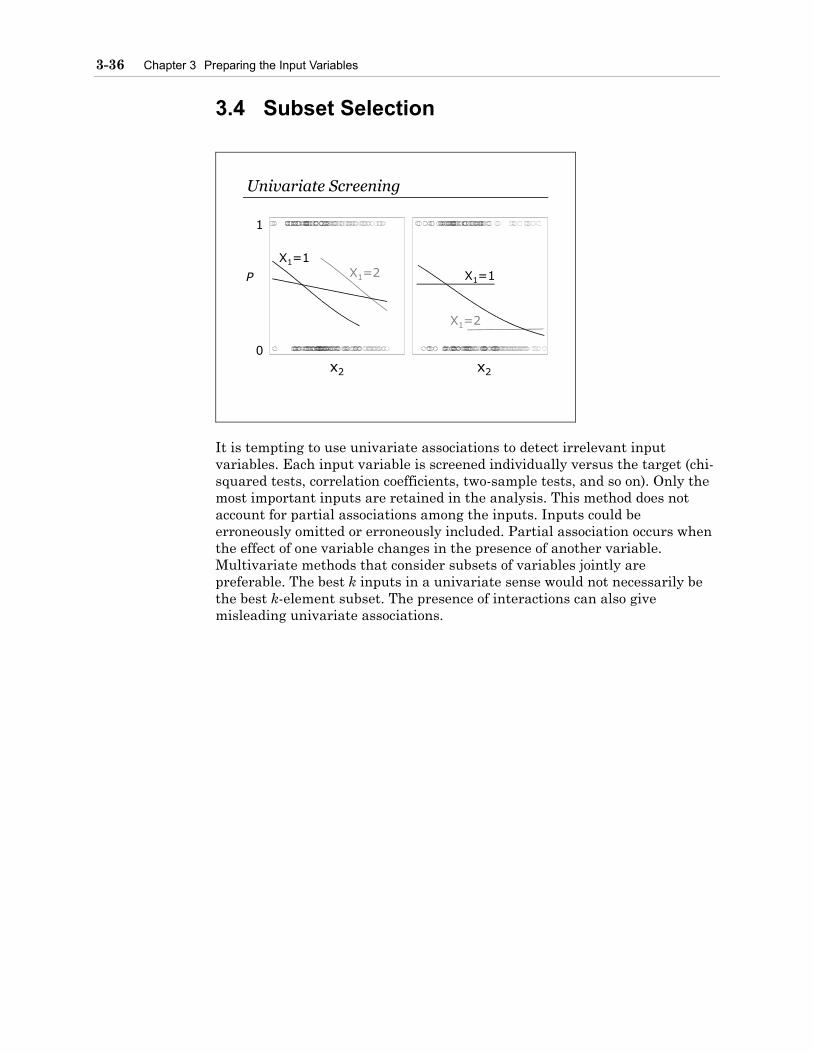
3-36 Chapter 3 Preparing the Input Variables
3.4 Subset Selection
Univariate Screening
P
1
0x2 x2
X1=1X1=2 X1=1
X1=2
It is tempting to use univariate associations to detect irrelevant input variables. Each input variable is screened individually versus the target (chi-squared tests, correlation coefficients, two-sample tests, and so on). Only the most important inputs are retained in the analysis. This method does not account for partial associations among the inputs. Inputs could be erroneously omitted or erroneously included. Partial association occurs when the effect of one variable changes in the presence of another variable. Multivariate methods that consider subsets of variables jointly are preferable. The best k inputs in a univariate sense would not necessarily be the best k-element subset. The presence of interactions can also give misleading univariate associations.

3.4 Subset Selection 3-37
Demonstration 9
Even after variable clustering, some further variable reduction may be needed prior to using the variable selection techniques in the LOGISTIC procedure. Very liberal univariate screening may be helpful when the number of clusters created in the VARCLUS procedure is still relatively large. Since some of the variable selection techniques use the full model, eliminating clearly irrelevant variables (for example, p-values greater than .50) will stabilize the full model and may improve the variable selection technique without much risk of eliminating important input variables. Keep in mind that univariate screening can give misleading results when there are partial associations. This problem was minimized because the screening was done after PROC VARCLUS, and was used in eliminating clearly irrelevant variables.
The CORR procedure can be used for univariate screening. The SPEARMAN option requests Spearman correlation statistics, which is a correlation of the ranks of the input variables with the binary target. The Spearman correlation statistic was used rather than the Pearson correlation statistic because Spearman is less sensitive to nonlinearities and outliers. However, when variables are not monotonically related to each other, the Spearman correlation statistic can miss important associations. A general and robust similarity measure is Hoeffding’s D (requested by the HOEFFDING option) which will detect a wide variety of associations between two variables. Hoeffding’s D statistic has values between –0.5 to 1, but if there are many ties, smaller values may result. The RANK option prints the correlation coefficients for each variable in order from highest to lowest.
A useful table would compare the rank order of the Spearman correlation statistic to the rank order of the Hoeffding’s D statistic. If the Spearman rank is low but the Hoeffding’s D rank is high, then the association is probably not monotonic. Empirical logit plots (discussed in a later section) could be used to investigate this type of relationship.
The output object for the table of Spearman correlation statistics is called SPEARMANCORR while the output object for the table of Hoeffding’s D statistics is called HOEFFDINGCORR. ods listing close; ods output spearmancorr=spearman hoeffdingcorr=hoeffding; proc corr data=imputed spearman hoeffding rank; var &reduced; with ins; run; ods listing;

3-38 Chapter 3 Preparing the Input Variables
The variable names in the SAS data sets SPEARMAN and HOEFFDING are in the variables BEST1 through BEST40, the correlation statistics are in the variables R1 through R40, and the p-values are in the variables P1 through P40. Therefore, a DATA step is used to transpose the variables to observations. data spearman1(keep=variable scorr spvalue ranksp); length variable $ 8; set spearman; array best(40) best1--best40; array r(40) r1--r40; array p(40) p1--p40; do i=1 to 40; variable=best(i); scorr=r(i); spvalue=p(i); ranksp=i; output; end; run; data hoeffding1(keep=variable hcorr hpvalue rankho); length variable $ 8; set hoeffding; array best(40) best1--best40; array r(40) r1--r40; array p(40) p1--p40; do i=1 to 40; variable=best(i); hcorr=r(i); hpvalue=p(i); rankho=i; output; end; run;
The two data sets are then sorted by the variable names and merged by the variable names.
proc sort data=spearman1; by variable; run; proc sort data=hoeffding1; by variable; run; data correlations; merge spearman1 hoeffding1; by variable; run;

3.4 Subset Selection 3-39
The final data set is sorted by the rank of the Spearman correlation statistic and then a table is generated showing the rank and associated statistics of the Spearman correlations and Hoeffding’s D statistics. proc sort data=correlations; by ranksp; run; proc print data=correlations label split='*'; var variable ranksp rankho scorr spvalue hcorr hpvalue; label ranksp = 'Spearman rank*of variables' scorr = 'Spearman Correlation' spvalue = 'Spearman p-value' rankho = 'Hoeffding rank*of variables' hcorr = 'Hoeffding Correlation' hpvalue = 'Hoeffding p-value'; run;
Spearman rank Hoeffding rank Spearman Obs variable of variables of variables Correlation 1 SAVBAL 1 1 0.25031 2 CD 2 4 0.20264 3 MMBAL 3 9 0.16066 4 SAV 4 3 0.15164 5 ATM 5 5 -0.12247 6 IRABAL 6 17 0.10995 7 PHONE 7 12 -0.10400 8 INV 8 22 0.09838 9 MMCRED 9 20 0.09509 10 CHECKS 10 7 -0.09015 11 brclus1 11 10 0.08189 12 CCPURC 12 15 0.08173 13 POSAMT 13 13 -0.07804 14 miphone 14 16 -0.07436 15 INVBAL 15 27 0.07277 16 SDB 16 18 0.07256 17 CCBAL 17 11 0.07147 18 DIRDEP 18 14 -0.07037 19 ATMAMT 19 6 -0.06809 20 NSFAMT 20 19 -0.06804 21 NSF 21 21 -0.06791 22 INAREA 22 23 -0.06049 Spearman Hoeffding Hoeffding Obs p-value Correlation p-value 1 0.00000 0.009764437 0.00001 2 0.00000 0.001876987 0.00001 3 0.00000 0.001117737 0.00001 4 0.00000 0.002395734 0.00001 5 0.00000 0.001480339 0.00001 6 0.00000 0.000198562 0.00001 7 0.00000 0.000615874 0.00001 8 0.00000 0.000059608 0.00761

3-40 Chapter 3 Preparing the Input Variables
9 0.00000 0.000119558 0.00025 10 0.00000 0.001239866 0.00001 11 0.00000 0.000638991 0.00001 12 0.00000 0.000240566 0.00001 13 0.00000 0.000445904 0.00001 14 0.00000 0.000222376 0.00001 15 0.00000 -.000011379 0.83466 16 0.00000 0.000175689 0.00001 17 0.00000 0.000632818 0.00001 18 0.00000 0.000402104 0.00001 19 0.00000 0.001410049 0.00001 20 0.00000 0.000119878 0.00025 21 0.00000 0.000114354 0.00033 22 0.00000 0.000015869 0.11424 Spearman rank Hoeffding rank Spearman Obs variable of variables of variables Correlation 23 brclus4 23 24 -0.06044 24 DDABAL 24 2 0.05611 25 DEPAMT 25 8 -0.04369 26 CASHBK 26 32 -0.04159 27 brclus3 27 30 -0.03224 28 INCOME 28 25 0.01441 29 ILSBAL 29 34 -0.01413 30 AGE 30 26 0.01252 31 micrscor 31 39 0.00895 32 miacctag 32 36 0.00533 33 MOVED 33 40 -0.00466 34 ACCTAGE 34 28 -0.00459 35 LORES 35 31 0.00408 36 CRSCORE 36 29 0.00407 37 LOC 37 37 0.00232 38 miincome 38 35 0.00159 39 HMOWN 39 33 -0.00060 40 MTG 40 38 -0.00042 Spearman Hoeffding Hoeffding Obs p-value Correlation p-value 23 0.00000 0.000006379 0.22409 24 0.00000 0.003101822 0.00001 25 0.00000 0.001179781 0.00001 26 0.00000 -.000033143 1.00000 27 0.00000 -.000022896 1.00000 28 0.00966 0.000002916 0.29081 29 0.01113 -.000037882 1.00000 30 0.02457 -.000000997 0.39375 31 0.10779 -.000043281 1.00000 32 0.33881 -.000041551 1.00000 33 0.40294 -.000043400 1.00000 34 0.40928 -.000015364 0.97453 35 0.46371 -.000026362 1.00000 36 0.46454 -.000017633 0.99778 37 0.67642 -.000042162 1.00000 38 0.77572 -.000038195 1.00000 39 0.91437 -.000034339 1.00000 40 0.93941 -.000042850 1.00000

3.4 Subset Selection 3-41
Since the goal is to eliminate the obviously irrelevant input variables, only the variables with Spearman correlation p-values of .50 or greater are eliminated (the criteria to use in eliminating variables is a subjective decision). Thus, four variables were eliminated from the analysis. These variables also had high p-values for Hoeffding’s D statistic.
Low ranks for Spearman and high ranks for Hoeffding’s D are found for the variables DDABAL, DEPAMT, and ATMAMT. Even though these variables do not have a monotonic relationship with INS, some other type of relationship is detected by Hoeffding’s D statistic. Empirical logit plots should be used to examine these relationships.
The %LET statement creates a macro variable called SCREENED that has the names of the variables remaining after the univariate screening method.
%let screened= savbal cd mmbal sav atm irabal phone inv mmcred checks brclus1 ccpurc posamt miphone invbal sdb ccbal dirdep atmamt nsfamt nsf inarea brclus4 ddabal depamt cashbk brclus3 income ilsbal age micrscor miacctag moved acctage lores crscore;

3-42 Chapter 3 Preparing the Input Variables
All Subsets
1110
3222
2k
Variable selection methods in regression are concerned with finding subsets of the inputs that are jointly important in predicting the target. The most thorough search would consider all possible subsets. This can be prohibitively expensive when the number of inputs, k, is large, as there are 2k possible subsets to consider.

3.4 Subset Selection 3-43
Stepwise Selection
123456
Stop
0
Stepwise variable selection is a much maligned yet heavily used subset selection method. Stepwise selection first searches the 1-input models and selects the best. It then searches the 2-input models that contain the input selected in the first step and selects the best. The model is incrementally built in this fashion until no improvement is made. There is also a backward portion of the algorithm where at each step, the variables in the current model can be removed if they have become unimportant. The usual criterion used for entry and removal from the model is the p-value from a significance test that the coefficient is zero, although other criterion can also be used. Note that in subset selection, the p-value is merely a tuning parameter that measures the relative strength of the candidate variables.
Stepwise selection was devised to give a computationally efficient alternative to examining all subsets. It is not guaranteed to find the best subset and it can be shown to perform badly in many situations (Harrell 1997).
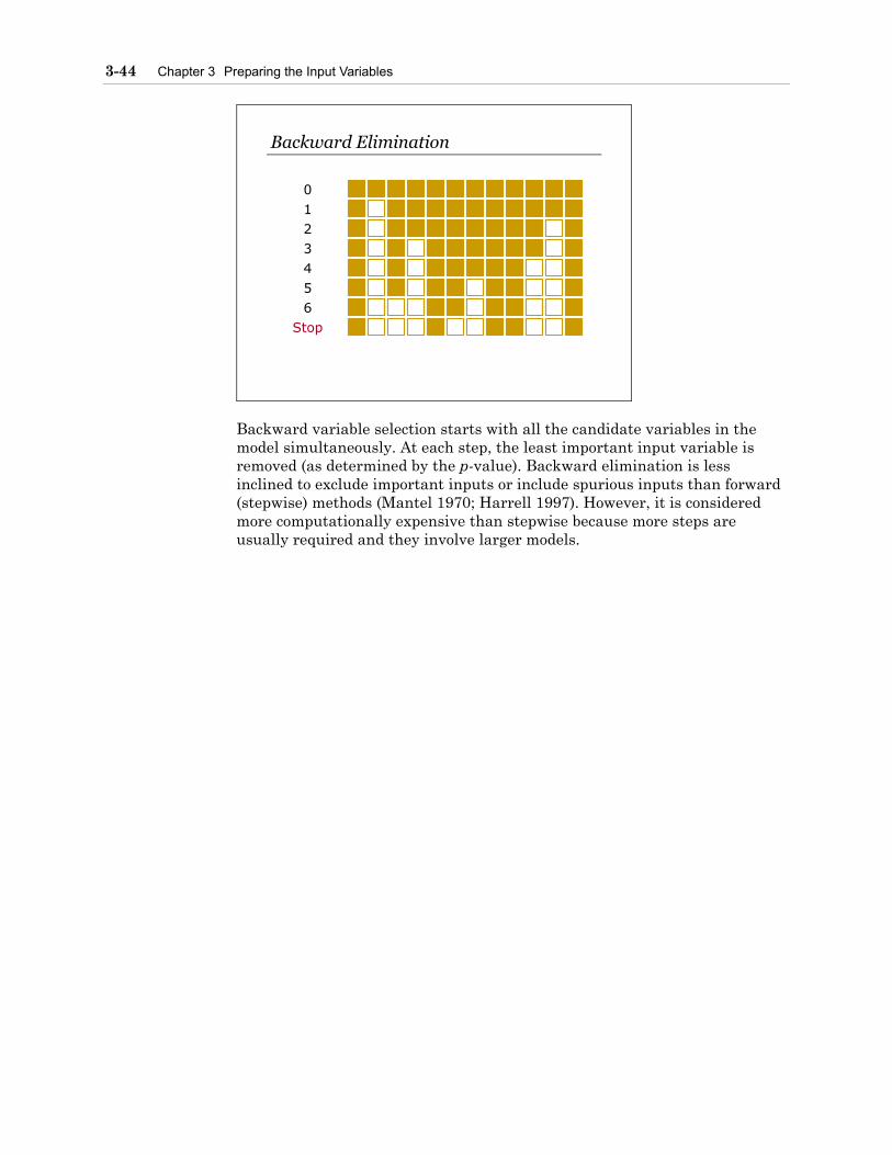
3-44 Chapter 3 Preparing the Input Variables
Backward Elimination
456
Stop
0123
Backward variable selection starts with all the candidate variables in the model simultaneously. At each step, the least important input variable is removed (as determined by the p-value). Backward elimination is less inclined to exclude important inputs or include spurious inputs than forward (stepwise) methods (Mantel 1970; Harrell 1997). However, it is considered more computationally expensive than stepwise because more steps are usually required and they involve larger models.

3.4 Subset Selection 3-45
Scalability in PROC LOGISTIC
0
15
30
45
60
25 50 75 100 150 200
Number of Variables
AllSubsets
Stepwise
Fast BackwardMin
ute
s
Most of the literature on the different subset selection methods has considered linear rather than logistic regression. The conventional wisdom regarding computation time is that
stepwise < backwards < all subsets.
However, logistic regression (as implemented by PROC LOGISTIC) gives a different story. For up to ≈60 inputs, the results are reversed
all subsets < backwards < stepwise.
For any number of inputs, backward elimination (with the FAST option) is more efficient than stepwise. (The above simulation was conducted with 50,000 cases and 200 intercorrelated inputs; 16 of the inputs were important, 6 strongly so.)
Logistic regression requires an iterative optimization algorithm. Each model fit is much more expensive than with linear regression. Each step in the stepwise algorithm requires iterative optimization. To find 16 variables (considering only the forward part of stepwise) would take 16k–17 separate nonlinear regressions, each of which might require several iterations. Stepwise logistic regression is a poor performer. Since its only universally acknowledged advantage is speed, there is little reason to prefer it for logistic regression (using PROC LOGISTIC).

3-46 Chapter 3 Preparing the Input Variables
All-subsets selection is executed in PROC LOGISTIC with the SELECTION=SCORE option (SAS Institute Inc. 1997). This method only requires that one model be fit (the full model). The results are then manipulated to calculate a score test for each possible combination of input variables. It also uses a branch and bound method for efficiently searching the many combinations. This method is the fastest until the number of possible combinations becomes unmanageable, at which point the performance acutely deteriorates. If redundant inputs are eliminated first (using variable clustering), then all-subsets selection can be a practical method for predictive modeling.
When combined with the FAST option, backward variable selection requires only a single logistic regression (SAS Institute Inc. 1997). PROC LOGISTIC uses the method of Lawless and Singhal (1978) to manipulate the full model fit to approximate fitting reduced models. The FAST option is extremely efficient because the model is not refitted for every variable removed. Fast backward elimination had the best overall performance, a linear increase in time as the number of inputs increased. Note that ordinary backwards (without the FAST option) would have been slower than stepwise.

3.4 Subset Selection 3-47
Demonstration 10
PROC LOGISTIC can be used to further reduce the number of input variables. In the MODEL statement, the SELECTION= option specifies the method – in this example, the backward elimination method. The FAST option uses the full model fit to approximate the remaining slope estimates for each subsequent elimination of a variable from the model. The SLSTAY option specifies the significance level for a variable to stay in the model in a backward elimination step. The significance level was chosen arbitrarily for illustrative purposes. proc logistic data=imputed des; class res; weight sampwt; model ins=&screened res / selection=backward fast slstay=.001; run;
Partial Output Summary of Backward Elimination
Effect Number Wald Step Removed DF In Chi-Square Pr > ChiSq 1 MMCRED 1 36 0.0058 0.9394 1 RES 2 35 0.3059 0.8582 1 CRSCORE 1 34 0.0554 0.8139 1 AGE 1 33 0.0541 0.8160 1 CCBAL 1 32 0.0720 0.7885 1 INVBAL 1 31 0.0817 0.7750 1 miacctag 1 30 0.1075 0.7430 1 LORES 1 29 0.1523 0.6964 1 INCOME 1 28 0.2077 0.6486 1 NSFAMT 1 27 0.3086 0.5785 1 MOVED 1 26 0.3515 0.5533 1 micrscor 1 25 0.3766 0.5394 1 SDB 1 24 0.5326 0.4655 1 IRABAL 1 23 0.8068 0.3691 1 DEPAMT 1 22 0.8307 0.3621 1 ILSBAL 1 21 0.9144 0.3390 1 NSF 1 20 1.1359 0.2865 1 CASHBK 1 19 1.2483 0.2639 1 POSAMT 1 18 1.3454 0.2461 1 brclus1 1 17 1.4111 0.2349 1 ACCTAGE 1 16 1.5698 0.2102 1 CCPURC 1 15 1.4997 0.2207 1 INAREA 1 14 1.5335 0.2156 1 brclus4 1 13 2.1359 0.1439 1 DIRDEP 1 12 2.4047 0.1210 1 CHECKS 1 11 7.3521 0.0067 1 brclus3 1 10 7.8062 0.0052 1 PHONE 1 9 10.4583 0.0012

3-48 Chapter 3 Preparing the Input Variables
Analysis of Maximum Likelihood Estimates Standard Parameter DF Estimate Error Chi-Square Pr > ChiSq Intercept 1 -4.1846 0.0801 2727.2611 <.0001 SAVBAL 1 0.000013 2.624E-6 24.5505 <.0001 CD 1 0.9654 0.1012 90.9924 <.0001 MMBAL 1 0.000040 6.076E-6 42.5514 <.0001 SAV 1 0.6714 0.0855 61.6991 <.0001 ATM 1 -0.5077 0.0866 34.4021 <.0001 INV 1 0.7313 0.1985 13.5756 0.0002 miphone 1 -0.5715 0.1381 17.1293 <.0001 ATMAMT 1 0.000034 7.013E-6 23.3099 <.0001 DDABAL 1 0.000013 3.663E-6 12.9517 0.0003
The results show that PROC LOGISTIC using the backward elimination method reduced the number of variables down from 37 to 9.
The SELECTION=SCORE option finds the best subsets of each model size. The number of models printed of each size is controlled by the BEST= option. Since the best subsets method does not support class variables, dummy variables for RES are created in a data step.
data imputed; set imputed; resr=(res='R'); resu=(res='U'); run; proc logistic data=imputed des; weight sampwt; model ins=&screened resr resu / selection=score best=1; run;
Partial Output Regression Models Selected by Score Criterion
Number of Score Variables Chi-Square Variables Included in Model 1 261.7275 SAVBAL 2 413.8070 SAVBAL CD 3 495.6601 SAVBAL CD MMBAL 4 535.4283 SAVBAL CD MMBAL DDABAL 5 562.1940 SAVBAL CD MMBAL SAV DDABAL 6 586.4394 SAVBAL CD MMBAL SAV INV DDABAL 7 609.6339 SAVBAL CD MMBAL SAV INV CHECKS DDABAL

3.4 Subset Selection 3-49
8 631.4205 SAVBAL CD MMBAL SAV ATM miphone ATMAMT DDABAL 9 651.0311 SAVBAL CD MMBAL SAV ATM INV miphone ATMAMT DDABAL 10 670.1744 SAVBAL CD MMBAL SAV ATM INV CHECKS miphone ATMAMT DDABAL 11 680.3776 SAVBAL CD MMBAL SAV ATM INV CHECKS miphone ATMAMT DDABAL brclus3
The score test statistic increases with model size. The Schwarz Bayes criterion (SBC) is often used for model selection. The SBC is essentially the –2 log likelihood plus a penalty term that increases as the model gets bigger. The penalty term for SBC is (k+1)⋅ln(n), where k is the number of variables in the model and n is the sample size. Smaller values of SBC are preferable. The score test statistic is asymptotically equivalent to the likelihood ratio statistic. The –2 log likelihood is a constant minus the likelihood ratio statistic. Thus, an SBC type statistic could be computed from the score statistic as –(score) + (k+1)⋅ln(n), where smaller values would be preferable.
When the SELECTION=SCORE option is used, output data sets are not available. Therefore, the output delivery system is used to create an output data set with the score statistic and the number of variables. The output objects with this information are called MODELINFO and BESTSUBSETS. ods listing close; ods output modelinfo=model bestsubsets=score; proc logistic data=imputed des; weight sampwt; model ins=&screened resr resu / selection=score best=1; run; ods listing; proc print data=model; run; Obs Description Value Label 1 Data Set WORK.IMPUTED 2 Response Variable INS Insurance Product 3 Number of Response Levels 2 4 Number of Observations 32264 5 Weight Variable sampwt 6 Sum of Weights 32263.999999 7 Link Function Logit 8 Optimization Technique Fisher's scoring
The value of interest is the number of observations. proc print data=score; run;

3-50 Chapter 3 Preparing the Input Variables
Partial Output control_ NumberOf Obs var Variables ScoreChiSq 1 1 261.7275 2 1 2 413.8070 3 1 3 495.6601 4 1 4 535.4283 Obs VariablesInModel 1 SAVBAL 2 SAVBAL CD 3 SAVBAL CD MMBAL 4 SAVBAL CD MMBAL DDABAL
The variables of interest to calculate SBC are NUMBEROFVARIABLES and SCORECHISQ from the SCORE data set and VALUE from the model data set.
The first DATA step selects one observation (the number of observations) and creates a macro variable OBS that contains the number of observations. The second DATA step computes the SBC statistic. data model; set model; if description = 'Number of Observations'; call symput('obs',value); run; data subset; set score; sbc=-scorechisq+log(&obs)*(numberofvariables+1); run; proc print data=subset; var sbc variablesinmodel; run;
Partial Output Obs sbc 1 -240.964 2 -382.662 3 -454.133 4 -483.520 5 -499.904 6 -513.767 7 -526.580 8 -537.985 9 -547.214 10 -555.976 11 -555.797 12 -548.682

3.4 Subset Selection 3-51
Obs VariablesInModel 1 SAVBAL 2 SAVBAL CD 3 SAVBAL CD MMBAL 4 SAVBAL CD MMBAL DDABAL 5 SAVBAL CD MMBAL SAV DDABAL 6 SAVBAL CD MMBAL SAV INV DDABAL 7 SAVBAL CD MMBAL SAV INV CHECKS DDABAL 8 SAVBAL CD MMBAL SAV ATM miphone ATMAMT DDABAL 9 SAVBAL CD MMBAL SAV ATM INV miphone ATMAMT DDABAL 10 SAVBAL CD MMBAL SAV ATM INV CHECKS miphone ATMAMT DDABAL 11 SAVBAL CD MMBAL SAV ATM INV CHECKS miphone ATMAMT DDABAL brclus3 12 SAVBAL CD MMBAL SAV ATM PHONE INV CHECKS miphone ATMAMT DDABAL brclus3
The output shows that the 10-variable model has the lowest SBC. This is a different model than the one selected in the backward method.
The %LET statement creates a macro variable called SELECTED that has the names of the variables selected from the fast backward elimination method.
%let selected=SAVBAL CD MMBAL SAV ATM INV miphone ATMAMT DDABAL;

3-52 Chapter 3 Preparing the Input Variables
3.5 Chapter Summary
Preparing the data for predictive modeling can be laborious. First, missing values need to be replaced with reasonable values. Missing indicator variables are also needed to accommodate whether the missingness is related to the target. If there are nominal input variables with numerous levels, the levels should be collapsed to reduce the likelihood of quasi-complete separation and to reduce the redundancy among the levels. Furthermore, if there are numerous input variables, variable clustering should be performed to reduce the redundancy among the variables. Finally, there are several selection methods in the LOGISTIC procedure to select a subset of variables. The Output Delivery System can be used to compute the SBC statistic for each selected model in the SELECTION=SCORE method.
To assist in identifying nonlinear associations, the Hoeffding’s D statistic can be used. A variable with a low rank in the Spearman correlation statistic but with a high rank in the Hoeffding’s D statistic may indicate that the association with the target is nonlinear.
General form of PROC STDIZE:
PROC STDIZE DATA=SAS-data-set <options>; VAR variables; RUN;
General form of PROC CLUSTER:
PROC CLUSTER DATA=SAS-data-set <options>; FREQ variable;
VAR variable; ID variable; RUN;
General form of PROC VARCLUS:
PROC VARCLUS DATA=SAS-data-set <options>; VAR variables; RUN;

Chapter 4 Classifier Performance
4.1 Honest Assessment....................................................................................................4-2
Demonstration 11............................................................................................................4-5
4.2 Misclassification .......................................................................................................4-17
Demonstration 12..........................................................................................................4-23
4.3 Allocation Rules........................................................................................................4-30
Demonstration 13..........................................................................................................4-35
4.4 Overall Predictive Power..........................................................................................4-36
Demonstration 14..........................................................................................................4-39
4.5 Chapter Summary.....................................................................................................4-41

4-2 Chapter 4 Classifier Performance
4.1 Honest Assessment
x2
x1
red →← blue
TrainingAccuracy = 70%
x2
red →← blue
TestAccuracy = 47%
The Optimism Principle
Evaluating the performance of a classifier on the same data used to train the classifier usually leads to an optimistically biased assessment.
For example, the above classifier was fit (or more properly overfit) to a 10 case data set. It correctly classified 70% of the cases. However, when the same classification rule was applied to 100 new cases from the same distribution, only 47% were correctly classified. This is called overfitting. The model was overly sensitive to peculiarities of the particular training data, in addition to true features of their joint distribution.
The more flexible the underlying model and less plentiful the data, the more that overfitting is a problem. When a relatively inflexible model like (linear) logistic regression is fitted to massive amounts of data, overfitting may not be a problem (Hand 1997). However, the chance of overfitting is increased by variable selection methods and supervised input preparation (such as collapsing levels of nominal variables based on associations with the target). It is prudent to assume overfitting until proven otherwise.
Large differences between the performance on the training and test sets usually indicate overfitting.

4.1 Honest Assessment 4-3
Data Splitting
ComparisonSelectionTuning
FinalAssessment
ValidationValidationValidation
TestTestTest
TrainingTrainingTraining
The simplest strategy for correcting the optimistic bias is to holdout a portion of the development data for assessment. The model is fit to the remainder (training data set) and performance is evaluated on the holdout portion (test data set). Usually from one-fourth to one-half of the development data is used as a test set (Picard and Berk 1990). After assessment, it is common practice to refit the final model on the entire undivided data set.
When the holdout data is used for comparing, selecting, and tuning models and the chosen model is assessed on the same data set that was used for comparison, then the optimism principle again applies. In this situation, the holdout sample is more correctly called a validation data set, not a test set. The test set is used for a final assessment of a fully specified classifier (Ripley 1996). If model tuning and a final assessment are both needed, then the data should be split three ways into training, validation, and test sets.

4-4 Chapter 4 Classifier Performance
Other Approaches
A B C D E
TrainBCDEACDEABDEABCEABCD
ValidateABCDE
1)2)3)4)5)
Data splitting is a simple but costly technique. When data is scarce, it is inefficient to use only a portion for training. Furthermore, when the test set is small, the performance measures may be unreliable because of high variability. For small and moderate data sets, ν-fold cross-validation (Breiman et al. 1984; Ripley 1996; Hand 1997) is a better strategy. In 5-fold cross-validation, for instance, the data would be split into five equal sets. The entire modeling process would be redone on each four-fifths of the data using the remaining one-fifth for assessment. The five assessments would then be averaged. In this way, all the data is used for both training and assessment.
Another approach that is frugal with the data is to assess the model on the same data set that was used for training but to penalize the assessment for optimism (Ripley 1996). The appropriate penalty can be determined theoretically or using computationally intensive methods such as the bootstrap.

4.1 Honest Assessment 4-5
Demonstration 11
The objective is to split the data into training and validation sets. The model and all the input preparation steps then need to be redone on the training set. The validation data will be used for assessment. Consequently, it needs to be treated as if it were truly new data where the target is unknown. The results of the analysis on the training data need to be applied to the validation data, not recalculated.
Several input-preparation steps can be done before the data is split. Creating missing indicators should be done on the full development data because the results will not change. The offset variable is also created before the data is split to get the best estimate of the proportion of events.
%let pi1=.02; data develop; set read.ins; run; %let inputs=ACCTAGE DDA DDABAL DEP DEPAMT CASHBK CHECKS DIRDEP NSF NSFAMT PHONE TELLER ATM ATMAMT POS POSAMT CD CDBAL IRA IRABAL LOC LOCBAL INV INVBAL ILS ILSBAL MM MMBAL MMCRED MTG MTGBAL SAV SAVBAL CC CCBAL CCPURC SDB INCOME HMOWN LORES HMVAL AGE CRSCORE MOVED INAREA; proc means data=develop noprint; var ins; output out=sum mean=rho1; run; data sum; set sum; call symput('rho1',rho1); run; data develop; set develop; off=log(((1-&pi1)*&rho1)/(&pi1*(1-&rho1))); run;

4-6 Chapter 4 Classifier Performance
data develop1(drop=i); set develop; array mi{*} miacctag miphone mipos miposamt miinv miinvbal micc miccbal miccpurc miincome mihmown milores mihmval miage micrscor; array x{*} acctage phone pos posamt inv invbal cc ccbal ccpurc income hmown lores hmval age crscore; do i=1 to dim(mi); mi{i}=(x{i}=.); end; run;
A DATA step is used to split DEVELOP into TRAIN and VALIDATE. The variable U is created using the RANUNI function, which generates pseudo-random numbers from a uniform distribution on the interval (0,1). The RANUNI function argument is an initialization seed. Using a particular number, greater than zero, will produce the same split each time the DATA step is run. If the seed was zero, then the data would be split differently each time the DATA step was run. The IF statement puts approximately 67% of the data into TRAIN and approximately 33% of the data into VALIDATE because on average 33% of the values of a uniform random variable are greater than 0.67.
data train(drop=u) validate(drop=u); set develop1; u=ranuni(27513); if u<=.67 then output train; else output validate; run;
All other input preparation steps are done after the split, on the training data only, because the validation data is treated as if it were truly new cases. This is imperative for supervised methods such as collapsing the levels of BRANCH based on its association with INS. It could be argued that unsupervised methods, such as median imputation, could be done on DEVELOP because they do not involve INS. This example presents a cautious approach and does not involve the validation data at all.
proc stdize data=train reponly method=median out=train1; var &inputs; run; proc means data=train1 noprint nway; class branch; var ins; output out=levels mean=prop; run;

4.1 Honest Assessment 4-7
ods output clusterhistory=cluster; proc cluster data=levels method=ward outtree=fortree; freq _freq_; var prop; id branch; run; ods listing;
Cluster History
T i NCL -------Clusters Joined-------- FREQ SPRSQ RSQ e 18 B5 B6 2840 0.0000 1.00 17 B10 B13 538 0.0000 1.00 16 B8 B9 1233 0.0000 1.00 15 B1 B4 5639 0.0000 1.00 14 CL17 B19 719 0.0000 1.00 13 CL15 B18 6000 0.0000 1.00 12 B11 B17 742 0.0000 1.00 11 B12 B7 1314 0.0000 1.00 10 B3 CL16 3129 0.0001 1.00 9 CL14 CL18 3559 0.0003 .999 8 CL12 CL11 2056 0.0012 .998 7 CL13 CL10 9129 0.0024 .996 6 B14 B15 2194 0.0128 .983 5 CL7 CL9 12688 0.0138 .969 4 CL8 B2 5657 0.0149 .954 3 CL6 B16 3228 0.0408 .914 2 CL5 CL4 18345 0.1588 .755 1 CL2 CL3 21573 0.7548 .000
proc freq data=train1 noprint; tables branch*ins / chisq; output out=chi(keep=_pchi_) chisq; run; data cutoff; if _n_ = 1 then set chi; set cluster; chisquare=_pchi_*rsquared; degfree=numberofclusters-1; logpvalue=logsdf('CHISQ',chisquare,degfree); run; proc plot data=cutoff; plot logpvalue*numberofclusters/vpos=30; run;

4-8 Chapter 4 Classifier Performance
The results of the cluster analysis now indicate four clusters is the optimum solution.
proc means data=cutoff noprint; var logpvalue; output out=small minid(logpvalue(numberofclusters))=ncl; run; data small; set small; call symput('ncl',ncl); run; proc tree data=fortree nclusters=&ncl out=clus h=rsq; id branch; run;

4.1 Honest Assessment 4-9
proc sort data=clus; by clusname; run; proc print data=clus; by clusname; id clusname; run;

4-10 Chapter 4 Classifier Performance
CLUSNAME BRANCH CLUSTER B16 B16 4 CL4 B11 2 B17 2 B12 2 B7 2 B2 2 CL5 B5 1 B6 1 B10 1 B13 1 B8 1 B9 1 B1 1 B4 1 B19 1 B18 1 B3 1 CL6 B14 3 B15 3
Three dummy variables are created and cluster 2 is made the reference level.
data train1; set train1; brclus1=(branch in ('B5','B6','B10','B13','B8','B9', 'B1','B4','B19','B18','B3')); brclus2=(branch in ('B14','B15')); brclus3=(branch='B16'); run;
ods listing close; ods output clusterquality=summary rsquare(match_all)=clusters; proc varclus data=train1 maxeigen=.7 outtree=fortree short; var &inputs brclus1-brclus3 miacctag miphone mipos miposamt miinv miinvbal micc miccbal miccpurc miincome mihmown milores mihmval miage micrscor; run; ods listing; proc print data=summary; run;

4.1 Honest Assessment 4-11
Number MaxOne Of TotVar PropVar MinProp MaxSecond Min Minus Obs Clusters Explained Explained Explained EigVal RSquare RSquare 1 1 9.166653 0.1455 0.1455 5.098792 0.0000 _ 2 2 14.185882 0.2252 0.2229 3.144899 0.0000 1.0000 3 3 17.243340 0.2737 0.1364 2.520114 0.0000 1.3782 4 4 19.761410 0.3137 0.1364 2.491691 0.0000 1.1549 5 5 22.210018 0.3525 0.1948 1.963822 0.0000 1.1725 6 6 24.124263 0.3829 0.1948 1.945563 0.0000 1.1725 7 7 25.932093 0.4116 0.1948 1.609776 0.0000 1.1725 8 8 27.419784 0.4352 0.2121 1.528157 0.0000 1.2991 9 9 28.912670 0.4589 0.2121 1.515521 0.0000 1.3181 10 10 30.379211 0.4822 0.2121 1.468003 0.0000 1.3181 11 11 31.798899 0.5047 0.2714 1.367502 0.0000 1.2939 12 12 33.110198 0.5256 0.2088 1.307745 0.0002 1.2939 13 13 34.396277 0.5460 0.2088 1.260232 0.0002 1.3029 14 14 35.638807 0.5657 0.2088 1.219690 0.0002 1.3029 15 15 36.733651 0.5831 0.2088 1.120758 0.0002 1.1981 16 16 37.841062 0.6007 0.3545 1.019254 0.0002 1.1981 17 17 38.770836 0.6154 0.3545 1.000715 0.0017 1.1981 18 18 39.760853 0.6311 0.3545 0.999841 0.0017 1.1981 19 19 40.760568 0.6470 0.3545 0.999470 0.0017 1.1981 20 20 41.759972 0.6629 0.3545 0.998939 0.0044 1.1981 21 21 42.758883 0.6787 0.3545 0.997610 0.0110 1.1981 22 22 43.613247 0.6923 0.3545 0.995811 0.0110 1.2036 23 23 44.608725 0.7081 0.3545 0.994090 0.0130 1.2036 24 24 45.602714 0.7239 0.3545 0.993266 0.0373 1.2036 25 25 46.571658 0.7392 0.3617 0.991991 0.0984 1.2036 26 26 47.563649 0.7550 0.3617 0.968124 0.0984 1.2036 27 27 48.530277 0.7703 0.3617 0.959208 0.1443 1.2036 28 28 49.489485 0.7855 0.3617 0.947892 0.1443 1.2036 29 29 50.381093 0.7997 0.5021 0.915163 0.1443 1.2036 30 30 51.290307 0.8141 0.5021 0.915073 0.2672 0.8997 31 31 52.205380 0.8287 0.5021 0.894051 0.2672 0.8997 32 32 53.051875 0.8421 0.5754 0.863930 0.2757 0.8997 33 33 53.911511 0.8557 0.5754 0.849134 0.3540 0.6889 34 34 54.760645 0.8692 0.6040 0.791978 0.3540 0.6889 35 35 55.552624 0.8818 0.6183 0.774018 0.3540 0.6889 36 36 56.323764 0.8940 0.6183 0.754263 0.4142 0.6471 37 37 57.077954 0.9060 0.6267 0.746587 0.5486 0.4604 38 38 57.824542 0.9178 0.6643 0.671393 0.5486 0.4604
A total of 38 clusters are formed.
data _null_; set summary; call symput('ncl',trim(left(numberofclusters-2))); run; proc print data=clusters&ncl; run;

4-12 Chapter 4 Classifier Performance
V R a N S r C O e q i o w x u a n V n t a b t C a C C r l r l r l l e e o u i u o R L l s a s s a a O V t b t e t b b a e l e s i e s r r e r t o l 1 Cluster 1 brclus2 0.8182 0.1617 0.2169 2 miphone 0.9977 0.0912 0.0026 3 mipos 0.9977 0.0912 0.0026 4 miposamt 0.9977 0.0912 0.0026 5 miinv 0.9977 0.0912 0.0026 6 miinvbal 0.9977 0.0912 0.0026 7 micc 0.9977 0.0912 0.0026 8 miccbal 0.9977 0.0912 0.0026 9 miccpurc 0.9977 0.0912 0.0026 10 - Cluster 2 miincome 0.9935 0.0517 0.0069 11 mihmown 0.9616 0.0484 0.0403 12 milores 0.9935 0.0517 0.0069 13 mihmval 0.9935 0.0517 0.0069 14 miage 0.9239 0.0908 0.0837 15 - Cluster 3 DEP 0.8045 0.3480 0.2998 Checking Deposits 16 CHECKS 0.8045 0.1526 0.2306 Number of Checks 17 - Cluster 4 MM 0.9147 0.0704 0.0918 Money Market 18 MMBAL 0.8998 0.0448 0.1049 Money Market Balance 19 MMCRED 0.5486 0.0196 0.4604 Money Market Credits 20 - Cluster 5 MTGBAL 0.9774 0.1617 0.0270 Mortgage Balance 21 CCBAL 0.9774 0.1113 0.0254 Credit Card Balance 22 - Cluster 6 ILS 0.9951 0.0356 0.0051 Installment Loan 23 ILSBAL 0.9951 0.0355 0.0051 Loan Balance 24 - Cluster 7 HMOWN 0.8071 0.1300 0.2218 Owns Home 25 LORES 0.8071 0.0695 0.2074 Length of Residence 26 - Cluster 8 POS 0.9200 0.0714 0.0861 Number Point of Sale 27 POSAMT 0.9200 0.0601 0.0851 Amount Point of Sale 28 - Cluster 9 NSF 0.7571 0.0515 0.2561 Number Insufficient Fund 29 NSFAMT 0.7571 0.0367 0.2521 Amount NSF 30 - Cluster 10 INCOME 0.8420 0.0287 0.1627 Income 31 HMVAL 0.8420 0.3111 0.2294 Home Value 32 - Cluster 11 CD 0.7150 0.0226 0.2915 Certificate of Deposit 33 CDBAL 0.7150 0.0373 0.2960 CD Balance 34 - Cluster 12 CC 0.6895 0.1064 0.3475 Credit Card 35 CCPURC 0.6895 0.0579 0.3296 Credit Card Purchases 36 - Cluster 13 IRA 0.6643 0.0416 0.3503 Retirement Account 37 IRABAL 0.6643 0.0316 0.3467 IRA Balance

4.1 Honest Assessment 4-13
38 - Cluster 14 LOC 0.7260 0.0373 0.2846 Line of Credit 39 LOCBAL 0.7260 0.0699 0.2945 Line of Credit Balance 40 - Cluster 15 INAREA 1.0000 0.1140 0.0000 Local Address 41 - Cluster 16 INVBAL 1.0000 0.0228 0.0000 Investment Balance 42 - Cluster 17 brclus1 1.0000 0.0996 0.0000 43 - Cluster 18 micrscor 1.0000 0.0182 0.0000 44 - Cluster 19 MOVED 1.0000 0.0016 0.0000 Recent Address Change 45 - Cluster 20 miacctag 1.0000 0.0063 0.0000 46 - Cluster 21 DDABAL 1.0000 0.1305 0.0000 Checking Balance 47 - Cluster 22 TELLER 1.0000 0.1786 0.0000 Teller Visits 48 - Cluster 23 SAVBAL 1.0000 0.0697 0.0000 Saving Balance 49 - Cluster 24 CASHBK 1.0000 0.0045 0.0000 Number Cash Back 50 - Cluster 25 brclus3 1.0000 0.0719 0.0000 51 - Cluster 26 ACCTAGE 1.0000 0.0206 0.0000 Age of Oldest Account 52 - Cluster 27 SDB 1.0000 0.0122 0.0000 Safety Deposit Box 53 - Cluster 28 CRSCORE 1.0000 0.1949 0.0000 Credit Score 54 - Cluster 29 SAV 1.0000 0.0697 0.0000 Saving Account 55 - Cluster 30 DDA 1.0000 0.2988 0.0000 Checking Account 56 - Cluster 31 ATMAMT 1.0000 0.0444 0.0000 ATM Withdrawal Amount 57 - Cluster 32 PHONE 1.0000 0.0898 0.0000 Number Telephone Banking 58 - Cluster 33 AGE 1.0000 0.1949 0.0000 Age 59 - Cluster 34 INV 1.0000 0.0229 0.0000 Investment 60 - Cluster 35 DEPAMT 1.0000 0.1305 0.0000 Amount Deposited 61 - Cluster 36 MTG 1.0000 0.1384 0.0000 Mortgage 62 - Cluster 37 DIRDEP 1.0000 0.1306 0.0000 Direct Deposit 63 - Cluster 38 ATM 1.0000 0.1612 0.0000 ATM
A macro variable REDUCED is created with the names of the variables selected using the VARCLUS procedure.
%let reduced=MIPHONE MIINCOME CHECKS MM CCBAL ILSBAL LORES POSAMT NSFAMT INCOME CD CCPURC IRABAL LOC INAREA INVBAL BRCLUS1 MICRSCOR MOVED MIACCTAG DDABAL TELLER SAVBAL CASHBK BRCLUS3 ACCTAGE SDB CRSCORE SAV DDA ATMAMT PHONE AGE INV DEPAMT MTG DIRDEP ATM;
A backward elimination method is used on the unweighted data. Since the slope estimates are not effected by the offset variable, the offset variable is not needed. The significance level of the SLSTAY option is selected for illustrative purposes. This level should be chosen based on the model’s performance on the validation data set.
proc logistic data=train1 des; class res; model ins=&reduced res / selection=backward fast slstay=.001; run;

4-14 Chapter 4 Classifier Performance
Partial Output Summary of Backward Elimination
Effect Number Wald Step Removed DF In Chi-Square Pr > ChiSq 1 INAREA 1 38 0.0250 0.8745 1 AGE 1 37 0.0443 0.8333 1 miincome 1 36 0.0910 0.7629 1 MOVED 1 35 0.2325 0.6297 1 NSFAMT 1 34 0.3759 0.5398 1 INCOME 1 33 0.5084 0.4758 1 DEPAMT 1 32 0.5585 0.4549 1 DIRDEP 1 31 0.6158 0.4326 1 INVBAL 1 30 0.6854 0.4077 1 RES 2 29 1.8443 0.3977 1 CRSCORE 1 28 0.8173 0.3660 1 ILSBAL 1 27 1.3557 0.2443 1 LOC 1 26 1.9314 0.1646 1 POSAMT 1 25 2.7332 0.0983 1 micrscor 1 24 3.2578 0.0711 1 LORES 1 23 3.6393 0.0564 1 CCBAL 1 22 3.6756 0.0552 1 miacctag 1 21 3.6378 0.0565 1 SDB 1 20 5.0751 0.0243 1 IRABAL 1 19 6.9956 0.0082 1 MTG 1 18 8.1627 0.0043 1 CCPURC 1 17 5.8720 0.0154
Analysis of Maximum Likelihood Estimates
Standard Parameter DF Estimate Error Chi-Square Pr > ChiSq Intercept 1 -0.6655 0.0508 171.5643 <.0001 miphone 1 -0.5807 0.0549 111.9259 <.0001 CHECKS 1 -0.0232 0.00383 36.5607 <.0001 MM 1 0.8945 0.0491 331.5734 <.0001 CD 1 0.9866 0.0458 463.8760 <.0001 brclus1 1 0.1902 0.0359 28.1067 <.0001 DDABAL 1 0.000066 4.028E-6 267.6425 <.0001 TELLER 1 0.0705 0.00774 82.8502 <.0001 SAVBAL 1 0.000045 2.673E-6 280.2161 <.0001 CASHBK 1 -0.4903 0.1482 10.9515 0.0009 brclus3 1 -0.4159 0.0823 25.5718 <.0001 ACCTAGE 1 -0.0153 0.00261 34.4581 <.0001 SAV 1 0.5333 0.0360 219.8357 <.0001 DDA 1 -0.7617 0.0484 247.4212 <.0001 ATMAMT 1 0.000059 6.587E-6 81.3175 <.0001 PHONE 1 -0.1262 0.0185 46.7789 <.0001 INV 1 0.6025 0.0977 38.0585 <.0001 ATM 1 -0.2022 0.0388 27.1809 <.0001

4.1 Honest Assessment 4-15
Odds Ratio Estimates Point 95% Wald Effect Estimate Confidence Limits miphone 0.560 0.502 0.623 CHECKS 0.977 0.970 0.984 MM 2.446 2.221 2.693 CD 2.682 2.452 2.934 brclus1 1.209 1.127 1.298 DDABAL 1.000 1.000 1.000 TELLER 1.073 1.057 1.089 SAVBAL 1.000 1.000 1.000 CASHBK 0.612 0.458 0.819 brclus3 0.660 0.561 0.775 ACCTAGE 0.985 0.980 0.990 SAV 1.705 1.589 1.829 DDA 0.467 0.425 0.513 ATMAMT 1.000 1.000 1.000 PHONE 0.881 0.850 0.914 INV 1.827 1.508 2.212 ATM 0.817 0.757 0.881 Association of Predicted Probabilities and Observed Responses Percent Concordant 76.6 Somers' D 0.536 Percent Discordant 23.1 Gamma 0.537 Percent Tied 0.3 Tau-a 0.242 Pairs 105263012 c 0.768
The results show that PROC LOGISTIC using the backward elimination method reduced the number of variables down from 38 to 17. This reduction is less than the results of the backward elimination method on weighted data. This illustrates that the significance level for SLSTAY should not be chosen arbitrarily, but rather on a trial and error basis based on the model’s performance on the validation data set.
%let selected= miphone CHECKS MM CD brclus1 DDABAL TELLER SAVBAL CASHBK brclus3 ACCTAGE SAV DDA ATMAMT PHONE INV ATM;
Since only seventeen variables appear in the final model, all the steps necessary for scoring the validation data need only involve those seventeen. Consequently, one more PROC LOGISTIC is run to create an OUTEST= data set with the final parameter estimates. The offset variable is needed to correctly adjust the intercept.
proc logistic data=train1 des outest=betas noprint; model ins=&selected / offset=off; run;

4-16 Chapter 4 Classifier Performance
In the validation data set, missing values should be replaced with the medians from the training data set. Since three variables (ACCTAGE, PHONE, and INV) have missing values, PROC UNIVARIATE is used to create an output data set with the medians of the three variables. The PCTLPTS option requests the 50th percentile while the PCTLPRE option specifies the prefix for the variable names in the output data set.
proc univariate data=train1; var acctage phone inv; output out=median pctlpts=50 pctlpre=acctage phone inv; run;
The DATA step first combines values from a single observation in one data set (MEDIAN) with all of the observations in another data set (VALIDATE). Array X contains the variables with missing values and array MED contains the variables with the medians. The DO loop replaces the missing values with the medians. Furthermore, since 2 BRANCH clusters appeared in the final model, the DATA step also creates the necessary dummy variables.
data validate (drop=acctage50 phone50 inv50 i); if _n_ = 1 then set median; set validate; array x(*) acctage phone inv; array med(*) acctage50 phone50 inv50; do i=1 to dim(med); if x(i)=. then x(i)=med(i); end; brclus1=(branch in ('B5','B6','B10','B13','B8','B9', 'B1','B4','B19','B18','B3')); brclus3=(branch='B16'); run;

4.2 Misclassification 4-17
4.2 Misclassification
Confusion Matrix
TrueNegative
FalsePositive
FalseNegative
TruePositive
ActualNegative
PredictedNegative
PredictedPositive
ActualPositive
Predicted Class
Act
ual Cla
ss
0
1
0 1
Supervised classification does not usually end with an estimate of the posterior probability. An allocation rule corresponds to a threshold value (cutoff) of the posterior probability. For example, all cases with probabilities of default greater than .04 might be rejected for a loan. For a given cutoff, how well does the classifier perform?
The fundamental assessment tool is the confusion matrix. The confusion matrix is a crosstabulation of the actual and predicted classes. It quantifies the confusion of the classifier. The event of interest, whether it is unfavorable (like fraud, churn, or default) or favorable (like response to offer), is often called a positive, although this convention is arbitrary. The simplest performance statistics are accuracy
(true positives and negatives) / (total cases)
and error rate
(false positives and negatives) / (total cases).

4-18 Chapter 4 Classifier Performance
Sensitivity and PV+
TruePositive
PredictedPositive
ActualPositive
Predicted Class
Act
ual Cla
ss
0
1
0 1
Two specialized measures of classifier performance are sensitivity
(true positives) / (total actual positives)
and positive predicted value (PV+)
(true positives) / (total predicted positives).
The analogues to these measures for true negatives are specificity
(true negatives) / (total actual negatives)
and negative predicted value (PV–)
(true negatives) / (total predicted negatives).
Large sensitivities do not necessarily correspond to large values of PV+. Ideally, one would like large values of all these statistics. The context of the problem determines which of these measures is the primary concern. For example, a database marketer might be most concerned with PV+ because it gives the response rate for the customers that receive an offer. In contrast, a fraud investigator might be most concerned with sensitivity because it gives the proportion of frauds that would be detected.

4.2 Misclassification 4-19
ROC Curve
Sensitivity
1 — Specificity
00
1
1
cuto
ff
The receiver operating characteristic (ROC) curve was adapted from signal detection theory for the assessment of classifiers. The ROC curve displays the sensitivity and specificity for the entire range of cutoffs values. As the cutoff decreases, more and more cases are allocated to class 1, hence the sensitivity increases and specificity decreases. As the cutoff increases, more and more cases are allocated to class 0, hence the sensitivity decreases and specificity increases. Consequently, the ROC curve intersects (0,0) and (1,1). If the posterior probabilities were arbitrarily assigned to the cases, then the ratio of false positives to true positives would be the same as the ratio of the total actual negatives to the total actual positives. Consequently, the baseline (random) model is a 45° angle going through the origin. As the ROC curve bows above the diagonal, the predictive power increases. A perfect model would reach the (0,1) point where both sensitivity and specificity equal 1.

4-20 Chapter 4 Classifier Performance
Gains Chart
Depth (%)
00
1
10020 40 60 80
PV+.5
cutoff
The depth of a classification rule is the total proportion of cases that were allocated to class 1. The (cumulative) gains chart displays the positive predicted value and depth for a range of cutoff values. As the cutoff decreases, more and more cases are allocated to class 1, hence the depth increases and the PV+ approaches the marginal event rate. When the cutoff is minimum, then 100% of the cases are selected and the response rate is ρ1. As the cutoff increases the depth decreases. A model with good predictive power would have increasing PV+ (response rate) as the depth decreases. If the posterior probabilities were arbitrarily assigned to the cases, then the gains chart would be a horizontal line at ρ1.
The gains chart is widely used in database marketing to decide how deep in a database to go with a promotion. The simplest way to construct this curve is to sort and bin the predicted posterior probabilities (for example, deciles). The gains chart is easily augmented with revenue and cost information. The lift is PV+/ρ1, so for a given depth, there are (lift)× more responders targeted by the model than by random chance.
A plot of sensitivity versus depth is sometimes called a Lorentz curve, concentration curve, or a lift curve (although lift value is not explicitly displayed). This plot and the ROC curve are very similar because depth and 1–specificity are monotonically related.
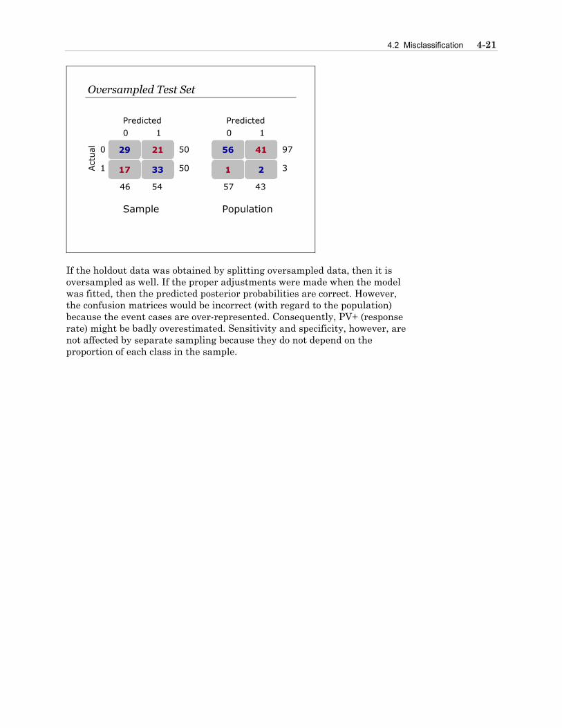
4.2 Misclassification 4-21
Oversampled Test Set
29 21
17 33
Predicted
Act
ual 0
1
0 1
46 54
50
50
56 41
1 2
Predicted0 1
57 43
97
3
Sample Population
If the holdout data was obtained by splitting oversampled data, then it is oversampled as well. If the proper adjustments were made when the model was fitted, then the predicted posterior probabilities are correct. However, the confusion matrices would be incorrect (with regard to the population) because the event cases are over-represented. Consequently, PV+ (response rate) might be badly overestimated. Sensitivity and specificity, however, are not affected by separate sampling because they do not depend on the proportion of each class in the sample.
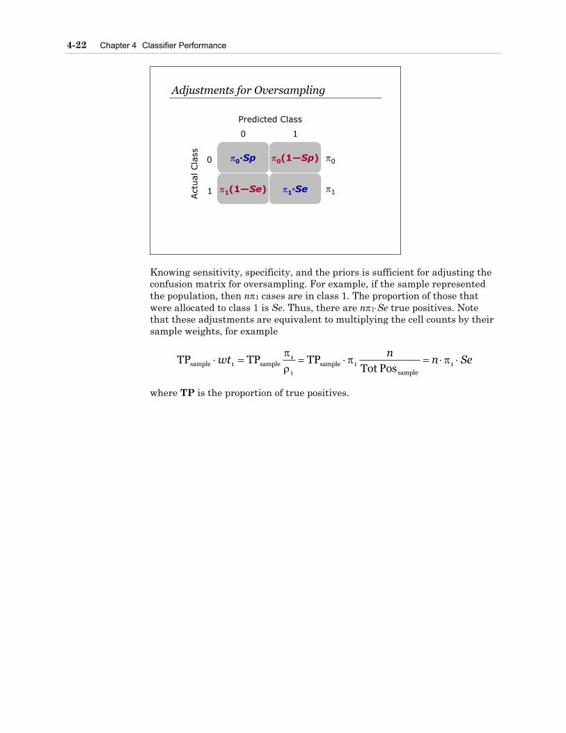
4-22 Chapter 4 Classifier Performance
Adjustments for Oversampling
π0·Sp π0(1—Sp)
π1(1—Se) π1·Se
Predicted Class
Act
ual
Cla
ss
0
1
0 1
π0
π1
Knowing sensitivity, specificity, and the priors is sufficient for adjusting the confusion matrix for oversampling. For example, if the sample represented the population, then nπ1 cases are in class 1. The proportion of those that were allocated to class 1 is Se. Thus, there are nπ1⋅Se true positives. Note that these adjustments are equivalent to multiplying the cell counts by their sample weights, for example
Senn
wt ⋅π⋅=π⋅=ρπ
=⋅ 1sample
1sample1
1sample1sample Pos Tot
TPTPTP
where TP is the proportion of true positives.

4.2 Misclassification 4-23
Demonstration 12
The performance measures need to be calculated on the validation data. One approach would be to use the SCORE procedure to score the validation data and then use DATA steps and the FREQ procedure to calculate misclassification measures for different cutoffs. An easier approach is to score the validation data inside the LOGISTIC procedure and use the OUTROC= data set, which contains many of the statistics necessary for assessment.
The INEST= option on the PROC LOGISTIC statement names the data set that contains initial parameter estimates for starting the iterative ML estimation algorithm. The MAXITER= option in the MODEL statement specifies the maximum number of iterations to perform. The combination of DATA=validation data, INEST=final estimates from training data, and MAXITER=0 causes PROC LOGISTIC to score, not refit, the validation data. The OFFSET= option is also needed since the offset variable was used when creating the final parameter estimates from the training data set.
The OUTROC= option creates an output data set with sensitivity (_SENSIT_) and one minus specificity (_1MSPEC_) calculated for a full range of cutoff probabilities (_PROB_). The other statistics in the OUTROC= data set are not useful when the data is oversampled. The two variables _SENSIT_ and _1MSPEC_ in the OUTROC= data set are correct whether or not the validation data is oversampled. The variable _PROB_ is correct, provided the INEST= parameter estimates were corrected for oversampling using sampling weights. If they were not corrected or if they were corrected with an offset, then _PROB_ needs to be adjusted using the formula (shown in Section 2.2).
10*
01*
10*
ˆ)ˆ1(
ˆˆ
πρ+πρ−πρ
=ii
ii pp
pp
where *ˆip is the unadjusted estimate of the posterior probability (_PROB_).
proc logistic data=validate des inest=betas; model ins=&selected / maxiter=0 outroc=roc offset=off; run;

4-24 Chapter 4 Classifier Performance
Partial Output The LOGISTIC Procedure
Model Information Data Set WORK.VALIDATE Response Variable INS Insurance Product Number of Response Levels 2 Number of Observations 10691 Offset Variable off Link Function Logit Optimization Technique Fisher's scoring
Response Profile
Ordered Total Value INS Frequency 1 1 3718 2 0 6973 Intercept-Only Model Convergence Status Iteration limit reached without convergence. WARNING: Convergence was not attained in 0 iterations for the intercept-only model. You may want to increase the maximum number of iterations (MAXITER= option) or change the convergence criteria (ABSFCONV=, FCONV=, GCONV=, XCONV= options) in the MODEL statement. WARNING: The LOGISTIC procedure continues in spite of the above warning. Results of fitting the intercept-only model are based on the last maximum likelihood iteration. Validity of the model fit is questionable.

4.2 Misclassification 4-25
Analysis of Maximum Likelihood Estimates
Standard Parameter DF Estimate Error Chi-Square Pr > ChiSq Intercept 1 -3.9222 0.0730 2885.3835 <.0001 miphone 1 -0.5807 0.0768 57.1157 <.0001 CHECKS 1 -0.0232 0.00575 16.2183 <.0001 MM 1 0.8945 0.0724 152.8072 <.0001 CD 1 0.9866 0.0650 230.4287 <.0001 brclus1 1 0.1902 0.0512 13.7921 0.0002 DDABAL 1 0.000066 5.656E-6 135.7719 <.0001 TELLER 1 0.0705 0.0111 40.4899 <.0001 SAVBAL 1 0.000045 3.912E-6 130.8423 <.0001 CASHBK 1 -0.4903 0.1995 6.0382 0.0140 brclus3 1 -0.4160 0.1197 12.0827 0.0005 ACCTAGE 1 -0.0153 0.00375 16.7221 <.0001 SAV 1 0.5333 0.0512 108.4217 <.0001 DDA 1 -0.7617 0.0701 118.0218 <.0001 ATMAMT 1 0.000059 9.247E-6 41.2669 <.0001 PHONE 1 -0.1262 0.0267 22.4150 <.0001 INV 1 0.6025 0.1404 18.4253 <.0001 ATM 1 -0.2022 0.0553 13.3848 0.0003 off 1 1.0000 0 . . WARNING: The validity of the model fit is questionable.
Association of Predicted Probabilities and Observed Responses Percent Concordant 75.8 Somers' D 0.518 Percent Discordant 23.9 Gamma 0.520 Percent Tied 0.3 Tau-a 0.235 Pairs 25925614 c 0.759
proc print data=roc(obs=25); var _prob_ _sensit_ _1mspec_; run;
Obs _PROB_ _SENSIT_ _1MSPEC_ 1 0.99996 0.003228 .000143410 2 0.99983 0.003765 .000286821 3 0.99977 0.004034 .000286821 4 0.99963 0.004303 .000286821 5 0.99938 0.004841 .000286821 6 0.99908 0.005648 .000286821 7 0.99868 0.006186 .000286821 8 0.99859 0.006186 .000430231 9 0.99849 0.006186 .000573641 10 0.99819 0.006724 .000573641 11 0.99810 0.007531 .000573641 12 0.99797 0.007800 .000717051 13 0.99767 0.008338 .000717051 14 0.99719 0.008338 .000860462

4-26 Chapter 4 Classifier Performance
15 0.99701 0.008607 .000860462 16 0.99669 0.008607 .001003872 17 0.99604 0.009145 .001003872 18 0.99595 0.009414 .001003872 19 0.99491 0.009683 .001003872 20 0.99462 0.009952 .001003872 21 0.99436 0.010221 .001003872 22 0.99412 0.010490 .001003872 23 0.99381 0.010758 .001003872 24 0.99367 0.010758 .001147282 25 0.99315 0.011027 .001147282
Since the model used an offset variable, the _PROB_ values need to be adjusted to reflect the population.
Knowledge of the population priors and sensitivity and specificity is sufficient to fill in the confusion matrices. Several additional statistics can be calculated in a DATA step:
• TP = proportion of true positives • FN = proportion of false negatives • TN = proportion of true negatives • FP = proportion of false positives • POSPV = positive predicted value • NEGPV = negative predicted value • ACC = accuracy • DEPTH = proportion allocated to class 1 • LIFT = positive predicted value/π1.
Each row in the OUTROC= data set corresponds to a cutoff (_PROB_). The selected cutoffs occur where values of the estimated posterior probability change, provided the posterior probabilities are more than .0001 apart, otherwise they are grouped. Consequently, the maximum number of rows in the OUTROC= data set is 9999, but it is usually much less. The grouping can be made coarser by using the ROCEPS= option on the MODEL statement.
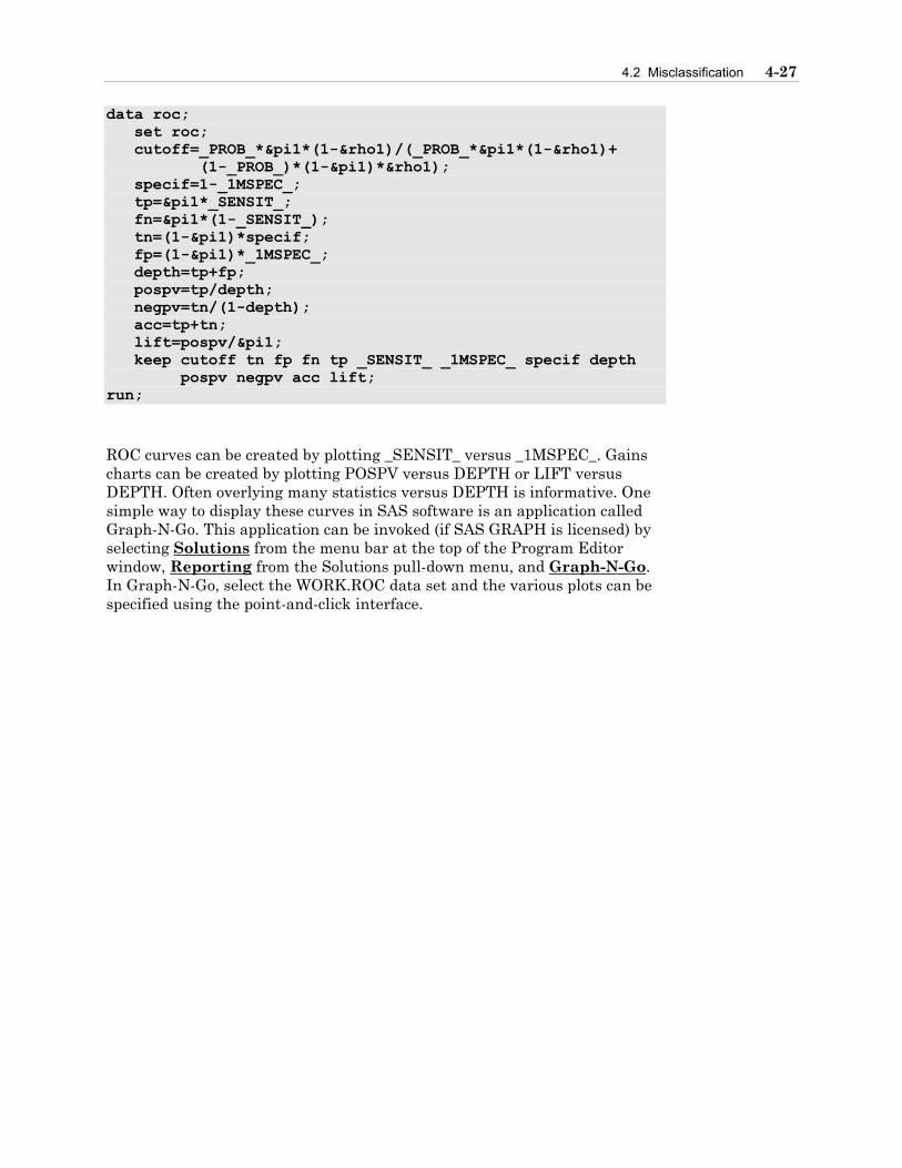
4.2 Misclassification 4-27
data roc; set roc; cutoff=_PROB_*&pi1*(1-&rho1)/(_PROB_*&pi1*(1-&rho1)+ (1-_PROB_)*(1-&pi1)*&rho1); specif=1-_1MSPEC_; tp=&pi1*_SENSIT_; fn=&pi1*(1-_SENSIT_); tn=(1-&pi1)*specif; fp=(1-&pi1)*_1MSPEC_; depth=tp+fp; pospv=tp/depth; negpv=tn/(1-depth); acc=tp+tn; lift=pospv/&pi1; keep cutoff tn fp fn tp _SENSIT_ _1MSPEC_ specif depth pospv negpv acc lift; run;
ROC curves can be created by plotting _SENSIT_ versus _1MSPEC_. Gains charts can be created by plotting POSPV versus DEPTH or LIFT versus DEPTH. Often overlying many statistics versus DEPTH is informative. One simple way to display these curves in SAS software is an application called Graph-N-Go. This application can be invoked (if SAS GRAPH is licensed) by selecting Solutions from the menu bar at the top of the Program Editor window, Reporting from the Solutions pull-down menu, and Graph-N-Go. In Graph-N-Go, select the WORK.ROC data set and the various plots can be specified using the point-and-click interface.

4-28 Chapter 4 Classifier Performance
Subsetting the range of plot values can be useful when the response rate is low. For example, the following lift chart is plotted for the top 30% of responders.
data roc1; set roc; if .001<depth<.3; run;

4.2 Misclassification 4-29

4-30 Chapter 4 Classifier Performance
4.3 Allocation Rules
Cutoffs
66 9
5 21
Se SpP
x1
x2
.84 .88
0 1
70 5
9 16.64 .93
57 18
1 24.96 .76
Different cutoffs produce different allocations and different confusion matrices. To determine the optimal cutoff, a performance criterion needs to be defined. If the goal were to increase the sensitivity of the classifier, then the optimal classifier would allocate all cases to class 1. If the goal were to increase specificity, then the optimal classifier would be to allocate all cases to class 0. For realistic data, there is a tradeoff between sensitivity and specificity. Higher cutoffs decrease sensitivity and increase specificity. Lower cutoffs decrease specificity and increase sensitivity.

4.3 Allocation Rules 4-31
Misclassification Costs
57 18
1 24
66 9
5 21
70 5
9 16
Total Cost
1*3 + 18 = 21
5*3 + 9 = 24
9*3 + 5 = 32
0 1
3 0
Predicted
Act
ual 0
1
0 1
A formal approach to determining the optimal cutoff uses statistical decision theory (McLachlan 1992; Ripley 1996; Hand 1997). The decision-theoretic approach starts by assigning misclassification costs (losses) to each type of error – false positives and false negatives. The optimal decision rule minimizes the total expected cost (risk).
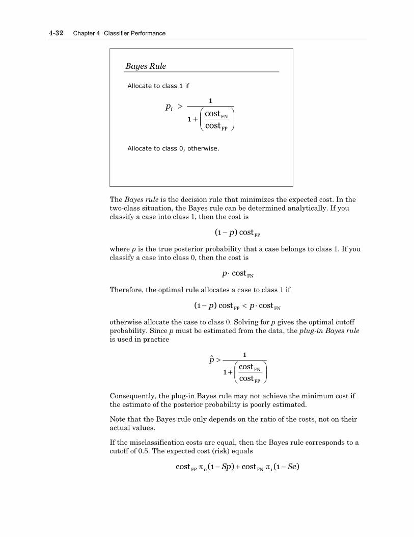
4-32 Chapter 4 Classifier Performance
Bayes Rule
+
>
FP
FN
costcost
1
1ip
Allocate to class 1 if
Allocate to class 0, otherwise.
The Bayes rule is the decision rule that minimizes the expected cost. In the two-class situation, the Bayes rule can be determined analytically. If you classify a case into class 1, then the cost is
FPcost)1( p−
where p is the true posterior probability that a case belongs to class 1. If you classify a case into class 0, then the cost is
FNcost⋅p
Therefore, the optimal rule allocates a case to class 1 if
FNFP costcost)1( ⋅<− pp
otherwise allocate the case to class 0. Solving for p gives the optimal cutoff probability. Since p must be estimated from the data, the plug-in Bayes rule is used in practice
+
>
FP
FN
cost
cost1
1p̂
Consequently, the plug-in Bayes rule may not achieve the minimum cost if the estimate of the posterior probability is poorly estimated.
Note that the Bayes rule only depends on the ratio of the costs, not on their actual values.
If the misclassification costs are equal, then the Bayes rule corresponds to a cutoff of 0.5. The expected cost (risk) equals
)1(cost)1(cost 1FN0FP SeSp −π+−π

4.3 Allocation Rules 4-33
When the cost ratio equals one, the expected cost is proportional to the error rate. A .5 cutoff tends to minimize error rate (maximize accuracy). Hand (1997) commented that
The use of error rate often suggests insufficiently careful thought about the real objectives….
When the target event is rare, the cost of a false negative is usually greater than the cost of a false positive. The cost of not soliciting a responder is greater than the cost of sending a promotion to someone who does not respond. The cost of accepting an applicant who will default is greater than the cost of rejecting someone who would pay-off the loan. The cost of approving a fraudulent transaction is greater than the cost of denying a legitimate one. Such considerations dictate cutoffs that are less (often much less) than .5.

4-34 Chapter 4 Classifier Performance
Cost Ratio
Sensitivity
mean(Se,Sp)
Specificity
CFN/CFP
Cutoff
π0/π1
π1
0
max(pi)
+∞
min(pi)
0
1
In many situations, it is difficult to precisely quantify the cost ratio, costFN/costFP. Examining the performance of a classifier over a range of cost ratios can be useful. A pertinent range of cost ratios is usually centered on the ratio of priors π0/π1. This corresponds to a cutoff of π1
1
1
01
1π=
ππ
+>p
For instance, if the nonevent cases were nine times more prevalent than the event cases, then a false negative would be nine times more costly than a false positive and the cutoff would be 0.1. When the cost ratio equals π0/π1, the expected cost is equivalent to the negative sum of sensitivity and specificity. The central cutoff, π1, tends to maximizes the mean of sensitivity and specificity. Because increasing sensitivity usually corresponds to decreasing specificity, the central cutoff tends to equalize sensitivity and specificity.
If separate samples were taken with equal allocation (50% events and 50% nonevents), then using the unadjusted cutoff of .5 on the biased sample is equivalent to using the central cutoff, π1, on the population.

4.3 Allocation Rules 4-35
Demonstration 13
Since the central cost ratio in this example is 49 (π0/π1 = .98/.02), an interesting range for the cost ratios might be from 30 to 90 (with more subject-matter knowledge a narrower range might be specified). The following DATA step adds the variable COSTRAT to the SAS data set ROC2 (the modified OUTROC= data set) and restricts the range of COSTRAT from 30 to 90.
data roc2; set roc; costrat=int((1-cutoff)/cutoff); if costrat ge 30 and costrat le 90; run;
In Graph-N-Go, COSTRAT can now be used as the X variable in the overlay plots. Restricting the range of the ROC2 data set when plotting variables versus COSTRAT usually makes the plots easier to read and interpret.
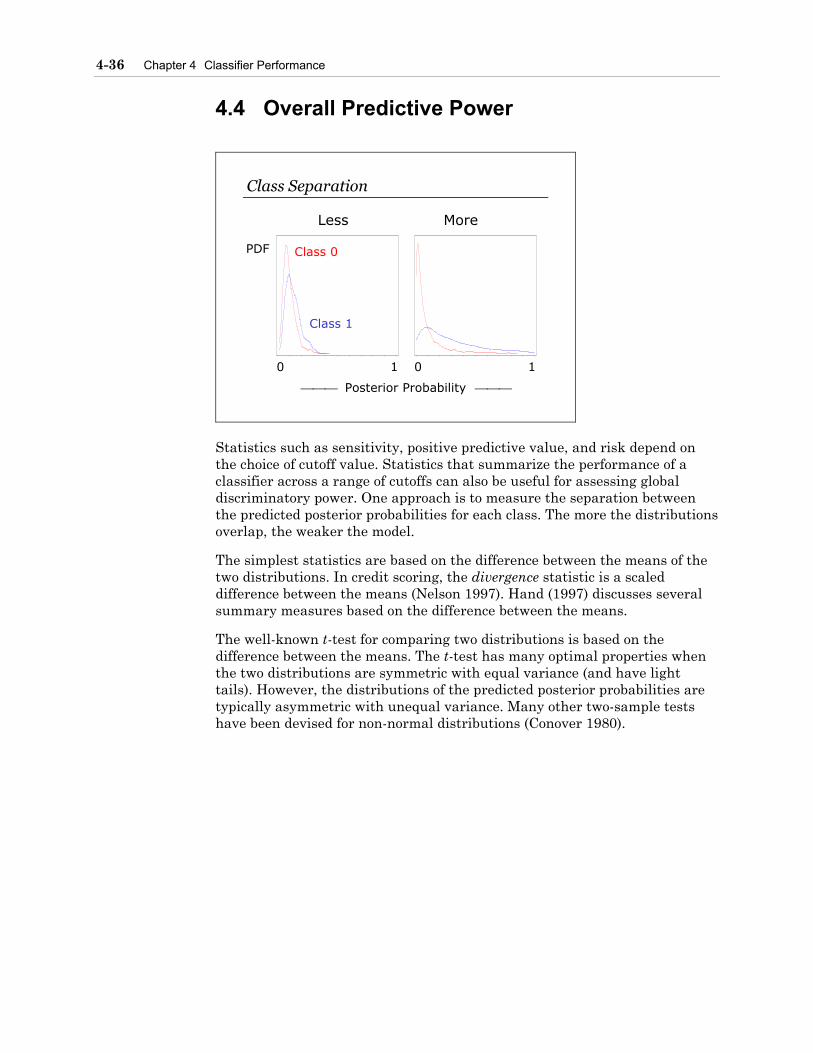
4-36 Chapter 4 Classifier Performance
4.4 Overall Predictive Power
Class Separation
Class 0
Class 1
Less More
Posterior Probability
0 1 0 1
Statistics such as sensitivity, positive predictive value, and risk depend on the choice of cutoff value. Statistics that summarize the performance of a classifier across a range of cutoffs can also be useful for assessing global discriminatory power. One approach is to measure the separation between the predicted posterior probabilities for each class. The more the distributions overlap, the weaker the model.
The simplest statistics are based on the difference between the means of the two distributions. In credit scoring, the divergence statistic is a scaled difference between the means (Nelson 1997). Hand (1997) discusses several summary measures based on the difference between the means.
The well-known t-test for comparing two distributions is based on the difference between the means. The t-test has many optimal properties when the two distributions are symmetric with equal variance (and have light tails). However, the distributions of the predicted posterior probabilities are typically asymmetric with unequal variance. Many other two-sample tests have been devised for non-normal distributions (Conover 1980).
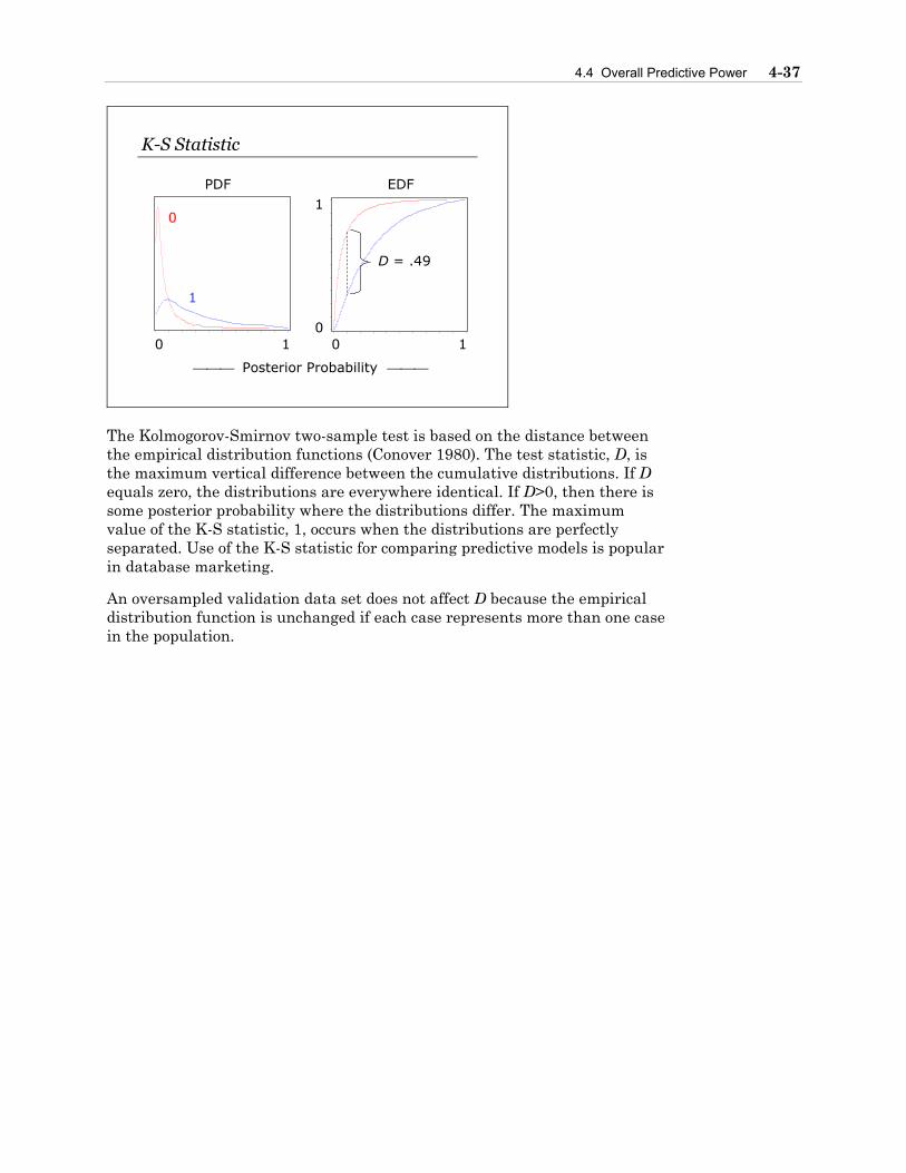
4.4 Overall Predictive Power 4-37
K-S Statistic
Posterior Probability
0 1
EDF
0 10
1
D = .49
0
1
The Kolmogorov-Smirnov two-sample test is based on the distance between the empirical distribution functions (Conover 1980). The test statistic, D, is the maximum vertical difference between the cumulative distributions. If D equals zero, the distributions are everywhere identical. If D>0, then there is some posterior probability where the distributions differ. The maximum value of the K-S statistic, 1, occurs when the distributions are perfectly separated. Use of the K-S statistic for comparing predictive models is popular in database marketing.
An oversampled validation data set does not affect D because the empirical distribution function is unchanged if each case represents more than one case in the population.

4-38 Chapter 4 Classifier Performance
Area Under the ROC Curve
PDF EDF ROC
D = .24
D = .49 c = .82
c = .66
The Kolmogorov-Smirnov two-sample test is sensitive to all types of differences between the distributions – location, scale, and shape. In the predictive modeling context, it could be argued that location differences are paramount. Because of its generality, the K-S test is not particularly powerful at detecting location differences. The most powerful nonparametric two-sample test is the Wilcoxon-Mann-Whitney test. Remarkably, the Wilcoxon-Mann-Whitney test statistic is also equivalent to the area under the ROC curve (Hand 1997).
The Wilcoxon version of this popular two-sample test is based on the ranks of the data. In the predictive modeling context, the predicted posterior probabilities would be ranked from smallest to largest. The test statistic is based on the sum of the ranks in the classes. The area under the ROC curve, c, can be determined from the rank-sum in class 1
01
1121
}1|{
)1(1
nn
nnR
c
n
yii
⋅
+−=
∑=
The first term in the numerator is the sum of the ranks in class 1.
A perfect ROC curve would be a horizontal line at one – that is, sensitivity and specificity would both equal one for all cutoffs. In this case, the c statistic would equal one. The c statistic technically ranges from zero to one, but in practice, it should not get much lower than ½. A perfectly random model, where the posterior probabilities were assigned arbitrarily, would give a 45° angle straight ROC curve that intersects the origin; hence, it would give a c statistic of 0.5.
Oversampling does not affect the area under the ROC curve because sensitivity and specificity are unaffected.
The area under the ROC curve is also equivalent to the Gini coefficient, which is used to summarize the performance of a Lorentz curve (Hand 1997).

4.4 Overall Predictive Power 4-39
Demonstration 14
The K-S statistic can be computed in the NPAR1WAY procedure using the scored validation data set. The SCORE procedure creates the variable INS2 for the logits since the variable INS already exists in the VALIDATE data set.
proc score data=validate out=scoval score=betas type=parms; var &selected; run; data scoval; set scoval; p=1/(1+exp(-ins2)); run;
The EDF and WILCOXON options in PROC NPAR1WAY request the Kolmogorov-Smirnov and Wilcoxon tests, respectively. The tests compare the values of the variable listed in the VAR statement between the groups listed in the CLASS statement.
proc npar1way edf wilcoxon data=scoval; class ins; var p; run;
Kolmogorov-Smirnov Test for Variable p Classified by Variable INS EDF at Deviation from Mean INS N Maximum at Maximum ƒƒƒƒƒƒƒƒƒƒƒƒƒƒƒƒƒƒƒƒƒƒƒƒƒƒƒƒƒƒƒƒƒƒƒƒƒƒƒƒƒƒƒƒƒƒƒƒƒƒ 1 3718 0.316568 -16.571730 0 6973 0.733257 12.100762 Total **** 0.588345 Maximum Deviation Occurred at Observation 6521 Value of p at Maximum = 0.018553 Kolmogorov-Smirnov Two-Sample Test (Asymptotic) KS 0.198453 D 0.416689 KSa 20.519520 Pr > KSa <.0001

4-40 Chapter 4 Classifier Performance
The results show that the two-sample Kolmogorov statistic D is 0.42, which represents the largest separation between the two cumulative distributions. The results of the Wilcoxon test can be used to compute the c statistic. However, this is automatically computed in the LOGISTIC procedure.
proc logistic data=validate des inest=betas; model ins=&selected / maxiter=0 offset=off; run;
Association of Predicted Probabilities and Observed Responses
Percent Concordant 75.8 Somers' D 0.518 Percent Discordant 23.9 Gamma 0.520 Percent Tied 0.3 Tau-a 0.235 Pairs 25925614 c 0.759

4.5 Chapter Summary 4-41
4.5 Chapter Summary
One of the most important steps in predictive modeling is to assess the performance of the model. To correct for the optimistic bias, a common strategy is to holdout a portion of the development data for assessment. The LOGISTIC procedure can then be used to score the data set used for assessment. Statistics that measure the predictive accuracy of the model include sensitivity and positive predicted value. Graphics such as the ROC curve, the gains chart, and the lift chart can also be used to assess the performance of the model.
If the assessment data set was obtained by splitting oversampled data, then the assessment data set needs to be adjusted. This can be accomplished by using the sensitivity, specificity, and the prior probabilities. Furthermore, if the OFFSET option was used, then the cutoff probabilities also need to be adjusted.
In predictive modeling, the ultimate use of logistic regression is to allocate cases to classes. To determine the optimal cutoff probability, the plug-in Bayes rule can be used. The information you need is the ratio of the costs of false negatives to the cost of false positives. This optimal cutoff will minimize the total expected cost.
When the target event is rare, the cost of a false negative is usually greater than the cost of a false positive. For example, the cost of not soliciting a responder is greater than the cost of sending a promotion to someone who does not respond. Such considerations dictate cutoffs that are usually much less than .50 (the cutoff that corresponds to equal misclassification costs).
A popular statistic that summarizes the performance of a model across a range of cutoffs is the Kolmogorov-Smirnov statistic. However, this statistic is not as powerful in detecting location differences as the Wilcoxon-Mann-Whitney test. Furthermore, the Wilcoxon-Mann-Whitney test statistic is equivalent to the area under the ROC curve (the c statistic). Thus, the c statistic should be used to assess the performance of a model across a range of cutoffs.
General form of PROC NPAR1WAY:
PROC NPAR1WAY DATA=SAS-data-set <options>; CLASS variable; VAR variable; RUN;

4-42 Chapter 4 Classifier Performance

Chapter 5 Nonlinearities and Interactions
5.1 Detection .....................................................................................................................5-2
Demonstration 15............................................................................................................5-4
5.2 Polynomials.................................................................................................................5-8
Demonstration 16..........................................................................................................5-11
5.3 Multilayer Perceptrons .............................................................................................5-14
Demonstration 16..........................................................................................................5-17
5.4 Chapter Summary.....................................................................................................5-19

5-2 Chapter 5 Nonlinearities and Interactions
5.1 Detection
Multivariate Relationships
LinearAdditive
NonlinearNonadditive
logit(p) logit(p)
x1 x2x1 x2
The curse of dimensionality makes detection of nonlinearities and interactions difficult in high dimensions. Decision trees (Breiman et al. 1984; Ripley 1996) are perhaps the most successful exploratory method for uncovering deviant data structure. Trees recursively partition the input space in order to isolate regions where the class composition is homogenous. Trees are flexible, interpretable, and scalable.
Univariate Smoothing
IIIIIIIIIIIIIIIIIIIIIIIIIIIIIIIIIIIIIIIIIIIIIIIIIIIIIIIIIIIIIIIIIIIIIIIIIIIIIIIIIIIIIIIIIIIIIIIIIIIIIIIIIIIIIIIIIIIIIIIIIIIIIIIIIIIIIIIIIIIIIIIIIIIIIIIIIIIIIIIIIIIIIIIIIIIIIIIIIIIIIIIIIIIIIIIIIIIIIIIIIIIIIIIIIIIIIIIIIIIIIIIIIIIIIIIIIIIIIIIIIIIIIIIIIIIIIIIIIIIIIIIIIIIIIIIIIIIIIIIIIIIIIIIIIIIIIIIIIIIIIIIIIIIIIIIIIIIIIIIIIIIIIIIIIIIIIIIIIIIIIIIIIIIIIIIIIIIIIIIIIIIIIIIIIIIIIIIIIIIIIIIIIIIIIIIIIIIIIIIIIII I II I
IIIIIIIIIIIIIIIIIIIII IIIII IIIIIIIIIIIIIIIIIIIIIIIIIIIIIIIIIIIIIIIIIIIIIIIIIIIII II III I I II IIII I
x x
0
0
1
Scatter Plot Empirical Logitsy
In regression analysis, it is standard practice to examine scatter plots of the target versus each input variable. When the target is binary, these plots are not very enlightening. A useful plot to detect nonlinear relationships is a plot of the empirical logits.

5.1 Detection 5-3
Empirical Logits
where
mi= number of events
Mi = number of cases
+−
+
2
2lni
ii
ii
MmM
Mm
Univariate plots of binary data need to be smoothed. A simple, scalable, and robust smoothing method is to plot empirical logits for quantiles of the input variables. These logits use a minimax estimate of the proportion of events in each bin (Duffy and Santner 1989). This eliminates the problem caused by zero counts and reduces variability.
The number of bins determines the amount of smoothing – the fewer bins, the more smoothing. One large bin would give a constant logit. For very large data sets and intervally-scaled inputs, 100 bins often works well. If the standard logistic model were true, then the plots should be linear. Sample variability can cause apparent deviations, particularly when the bin size is too small. However, serious nonlinearities, such as nonmonotonicity, are usually easy to detect.

5-4 Chapter 5 Nonlinearities and Interactions
Demonstration 15
To create a plot of the empirical logits versus an input variable, the input variable first needs to be binned. Use the RANK procedure with the GROUPS= option to bin variables automatically. The bins will be equal size (quantiles) except when the number of tied values exceeds the bin size, in which case the bin will be enlarged to contain all the tied values. The VAR statement lists the variable in the DATA= data set to be grouped. The RANKS statement names the variable representing the groups in the OUT= data set. If the RANKS statement is not used, the VAR variable is replaced by the groups.
%let var=ddabal; proc rank data=train1 groups=100 out=out; var &var; ranks bin; run; proc print data=out(obs=10); var &var bin; run;
OBS DDABAL BIN 1 1986.81 76 2 0.00 9 3 2813.45 83 4 1683.28 73 5 462.12 46 6 1772.13 74 7 1226.90 66 8 257.13 37 9 375.62 42 10 13.85 21
To compute the empirical logit the number of target event cases (INS=1) and total cases in each bin needs to be computed. The empirical logits are plotted against the mean of the input variable in each bin. This needs to be computed as well. Both tasks can be done in the MEANS procedure using the CLASS statement. The appropriate statistics (SUM and MEAN) need to be specified in the OUTPUT statement.

5.1 Detection 5-5
proc means data=out noprint nway; class bin; var ins &var; output out=bins sum(ins)=ins mean(&var)=&var; run; proc print data=bins(obs=10); run;
Obs bin _TYPE_ _FREQ_ ins ddabal 1 0 1 140 18 -33.8830 2 9 1 4002 2116 0.0000 3 19 1 172 19 2.6717 4 20 1 216 17 8.9133 5 21 1 216 29 17.1919 6 22 1 216 31 29.0083 7 23 1 215 28 41.5856 8 24 1 216 32 53.7313 9 25 1 216 33 67.4041 10 26 1 215 46 82.5093
The variable INS contains the number of events while the automatic variable _FREQ_ contains the bin size.
data bins; set bins; elogit=log((ins+(sqrt(_FREQ_)/2))/ (_FREQ_-ins+(sqrt(_FREQ_)/2))); run;
The empirical logits can be plotted in Graph-N-Go by selecting the WORK.BINS data set. The empirical logits for other input variables can be easily calculated by specifying the new variable in the initial %LET statement and rerunning the program.

5-6 Chapter 5 Nonlinearities and Interactions

5.1 Detection 5-7
Remedies
1. Hand-Crafted New Input Variables
2. Polynomial Models
3. Flexible Multivariate Function
Estimators
4. Do Nothing
1. Skilled and patient data analysts can accommodate nonlinearities in a logistic regression model by transforming or discretizing the input variables. This can become impractical with high-dimensional data and increases the risk of overfitting.
2. Section 5.2.
3. Methods such as classification trees, generalized additive models, projection pursuit, multivariate adaptive regression splines, radial basis function networks, and multilayer perceptrons (Section 5.3) are flexible alternatives to logistic regression (Hastie and Tibshirani 1990; Ripley 1996).
4. Standard (linear) logistic regression can produce powerful and useful classifiers even when the estimates of the posterior probabilities are poor. Often more flexible approaches do not show enough improvement to warrant the effort.

5-8 Chapter 5 Nonlinearities and Interactions
5.2 Polynomials
Degree
1st 2nd 3rd
Linear Quadratic Cubic
The classic approach to enhancing the flexibility of linear models is to add higher order (polynomial) terms. A linear model (first-degree polynomial) is planar. A quadratic model (second-degree polynomial) is a paraboloid or a saddle surface. Squared terms allow the effect of the inputs to be nonmonotonic. Moreover, the effects of one variable can change linearly across the levels of the other variables. Cubic models (third-degree polynomials) allow for a minimum and a maximum in each dimension. Moreover, the effect of one variable can change quadraticly across the levels of the other variables. Higher degree polynomials allow even more flexibility.

5.2 Polynomials 5-9
Terms
1st 2nd 3rdLinear Quadratic Cubic
x1x2x3
x1x1x2x2x3x3x1x2x1x3x2x3
x1x1x1x2x2x2x3x3x3x1x1x2x1x1x3x1x2x2x1x2x3x1x3x3
...
squared
2-way interactions
cubed
All polynomial models can be expressed as linear functions of the parameters, which allows them to be fitted using the same methods as first-degree polynomials. A polynomial model can be specified by including new terms to the model. The new terms are products of the original variables. A full polynomial model of degree d includes terms for all possible products involving up to d terms. For example, a full quadratic model with three inputs has nine terms
329318217236
225
2143322110 xxxxxxxxxxxx β+β+β+β+β+β+β+β+β+β
A quadratic polynomial contains squared and cross-product terms. The squared terms allow the effect of the inputs to be nonmonotonic. The cross product terms allow for interactions among the inputs. Cubic terms allow for even more flexibility.

5-10 Chapter 5 Nonlinearities and Interactions
Number of Terms
0 20 40 60 80 1000
1000
2000
3000
4000
5000
Input Dimension
Cubic
Quadratic
Linear
There are several drawbacks to using higher degree polynomials. Chief among them is the curse of dimensionality. The number of terms in a d-degree polynomial increases at a rate proportional to the number of dimensions raised to the d power (for example, the number of terms in a full quadratic model increases at a quadratic rate with dimension). Fitting and/or reducing such large polynomial models can be prohibitively difficult when there are many input variables.
Non-Local Behavior
II
I
II
I
IIIII
I
II
IIIII
I
IIIII
II
I
I
IIII
I
I
I
I
I
IIIIIIIIIIIIIIIIIIIIII
II
IIIIIIIIIII
I
IIIIIIIIIIIIIIIIIIIIIIIIIIIIIIIIIIIIIIIIIIIIIIIIIIIIIIIIIIIIIIIIIIIIIIIIIIIIIIIIIIIIIIIIIIIIIIIIIIIIIIIIIIIIIIIIIIIIIIIIIIIIIIIIIIIIIIIIIIIIIIIIIIIIIIIIIIIIIIIIIIIIIIIIIIIIIIIIIIIIIIIIIIIIIIIIIIIIIIIIIIIIIIIIIIIIIIIIIIIIIIIIIIIIIIIIIIIIIIIIII
I
IIIIIIIIIIIII
I
IIIIIIIIII
I
IIIIIIIIIIII
I
IIII
I
IIIIIIIIIIIIIIIIIIIIIIIIIIIIIIIIIII
I
I
I
III
I
IIIIIII
IIII
I
I
I
I
IIII
I
I
III
I
III
I
IIIIIIII
I
IIII
II
III
IIIII
II
I
I
I
I
I
II
I
IIII
I
I
I
IIII I I I
I
IIII
II
II I II I I
I
II III I I
Truth
QuarticFit
x
1
0
Another liability of higher-degree polynomials is their non-local behavior (Hastie and Tibshirani 1990; Magee 1998). For example, the influence that individual cases have on the predicted value at a particular point (the equivalent kernel) does not necessarily increase the closer they are to that particular point. Higher-degree polynomials are not reliable smoothers.

5.2 Polynomials 5-11
Demonstration 16
The detection of higher degree polynomial terms in high dimensions is a cumbersome task. One suggested approach is to include all the significant input variables and use a forward selection to detect any two-factor interactions and squared terms. This approach will miss the interactions and squared terms with non-significant input variables, but the number of possible two-factor interactions and squared terms is too large for the LOGISTIC procedure to assess.
In the MODEL statement in PROC LOGISTIC, the bar notation with @2 constructs a model with all the input variables and the two-factor interactions. The INCLUDE=n option includes the first n input variables in the MODEL statement in every model. Although this syntax will make PROC LOGISTIC evaluate redundant models, the loss in CPU time is minimal with a relatively few input variables.
proc logistic data=train1 des; model ins=miphone CHECKS MM CD brclus1 DDABAL TELLER SAVBAL CASHBK brclus3 ACCTAGE SAV DDA ATMAMT PHONE INV ATM miphone*miphone checks*checks MM*MM CD*CD brclus1*brclus1 DDABAL*DDABAL TELLER*TELLER SAVBAL*SAVBAL CASHBK*CASHBK brclus3*brclus3 acctage*acctage sav*sav dda*dda atmamt*atmamt phone*phone inv*inv atm*atm miphone|CHECKS|MM|CD|brclus1| DDABAL|TELLER|SAVBAL|CASHBK|brclus3| ACCTAGE|SAV|DDA|ATMAMT|PHONE|INV|ATM @2 / selection=forward include=17 slentry=.00001 ; run;
Partial Output Summary of Forward Selection Effect Number Score Step Entered DF In Chi-Square Pr > ChiSq 1 SAVBAL*SAVBAL 1 18 4493.6676 <.0001 2 DDABAL*DDABAL 1 19 1990.9810 <.0001 3 DDABAL*SAVBAL 1 20 495.9179 <.0001 4 ATMAMT*ATMAMT 1 21 141.4064 <.0001 5 SAVBAL*DDA 1 22 118.9575 <.0001 6 brclus1*ATMAMT 1 23 95.6299 <.0001 7 MM*SAVBAL 1 24 50.5022 <.0001 8 ACCTAGE*ACCTAGE 1 25 40.3526 <.0001 9 miphone*brclus1 1 26 35.9314 <.0001 10 CHECKS*DDABAL 1 27 35.2369 <.0001

5-12 Chapter 5 Nonlinearities and Interactions
11 DDABAL*PHONE 1 28 26.9956 <.0001 12 DDABAL*brclus3 1 29 26.6608 <.0001 13 MM*PHONE 1 30 25.7769 <.0001 14 SAV*DDA 1 31 25.7445 <.0001 15 MM*DDA 1 32 24.6602 <.0001 16 CASHBK*ACCTAGE 1 33 23.4510 <.0001
The forward selection method detected 16 significant higher order terms.
Analysis of Maximum Likelihood Estimates Standard Parameter DF Estimate Error Chi-Square Pr > ChiSq Intercept 1 -0.2010 0.0626 10.2909 0.0013 miphone 1 -0.7591 0.0658 132.9199 <.0001 CHECKS 1 -0.0203 0.00433 21.9244 <.0001 MM 1 0.6517 0.0763 72.9949 <.0001 CD 1 0.9693 0.0466 433.4879 <.0001 brclus1 1 0.0157 0.0398 0.1555 0.6933 DDABAL 1 0.000128 7.08E-6 325.6868 <.0001 TELLER 1 0.0803 0.00800 100.7011 <.0001 SAVBAL 1 0.000059 4.508E-6 172.2271 <.0001 CASHBK 1 -0.9286 0.1977 22.0641 <.0001 brclus3 1 -0.3362 0.0898 14.0185 0.0002 ACCTAGE 1 -0.0559 0.00645 75.0229 <.0001 SAV 1 0.0297 0.0833 0.1267 0.7219 DDA 1 -1.2624 0.0678 346.5681 <.0001 ATMAMT 1 0.000032 6.969E-6 20.4807 <.0001 PHONE 1 -0.1766 0.0228 60.1373 <.0001 INV 1 0.5739 0.0983 34.0658 <.0001 ATM 1 -0.1476 0.0415 12.6823 0.0004 DDABAL*DDABAL 1 -414E-12 3.75E-11 121.7575 <.0001 SAVBAL*SAVBAL 1 -23E-11 1.78E-11 167.9421 <.0001 ACCTAGE*ACCTAGE 1 0.00135 0.000204 43.7813 <.0001 ATMAMT*ATMAMT 1 -301E-12 4.12E-11 53.2335 <.0001 miphone*brclus1 1 0.7191 0.1206 35.5389 <.0001 CHECKS*DDABAL 1 -4.07E-6 5.967E-7 46.4636 <.0001 MM*SAVBAL 1 -0.00004 6.79E-6 32.5355 <.0001 DDABAL*SAVBAL 1 -1.84E-9 2.17E-10 72.0982 <.0001 DDABAL*brclus3 1 -0.00007 0.000015 22.4903 <.0001 CASHBK*ACCTAGE 1 0.1654 0.0401 17.0033 <.0001 MM*DDA 1 0.4947 0.0993 24.8192 <.0001 SAVBAL*DDA 1 0.000031 4.95E-6 38.0810 <.0001 SAV*DDA 1 0.5157 0.0905 32.4835 <.0001 brclus1*ATMAMT 1 0.000098 0.000011 74.8363 <.0001 MM*PHONE 1 0.2167 0.0643 11.3426 0.0008 DDABAL*PHONE 1 0.000031 6.551E-6 23.0239 <.0001 Association of Predicted Probabilities and Observed Responses Percent Concordant 78.2 Somers' D 0.566 Percent Discordant 21.6 Gamma 0.567 Percent Tied 0.2 Tau-a 0.256 Pairs 105263012 c 0.783

5.2 Polynomials 5-13
The final model now has 33 terms. The c statistic increased from .768 to .783. However, this model should be assessed using the validation data set because the inclusion of many higher order terms may increase the risk of overfitting.
proc logistic data=train1 des outest=betas; model ins=miphone CHECKS MM CD brclus1 DDABAL TELLER SAVBAL CASHBK brclus3 ACCTAGE SAV DDA ATMAMT PHONE INV ATM savbal*savbal ddabal*ddabal ddabal*savbal atmamt*atmamt savbal*dda brclus1*atmamt mm*savbal acctage*acctage miphone*brclus1 checks*ddabal ddabal*phone ddabal*brclus3 mm*phone sav*dda mm*dda cashbk*acctage; run; proc logistic data=validate des inest=betas; model ins=miphone CHECKS MM CD brclus1 DDABAL TELLER SAVBAL CASHBK brclus3 ACCTAGE SAV DDA ATMAMT PHONE INV ATM savbal*savbal ddabal*ddabal ddabal*savbal atmamt*atmamt savbal*dda brclus1*atmamt mm*savbal acctage*acctage miphone*brclus1 checks*ddabal ddabal*phone ddabal*brclus3 mm*phone sav*dda mm*dda cashbk*acctage / maxiter=0; run;
Association of Predicted Probabilities and Observed Responses Percent Concordant 77.0 Somers' D 0.543 Percent Discordant 22.7 Gamma 0.545 Percent Tied 0.3 Tau-a 0.246 Pairs 25925614 c 0.772
The validation c statistic is 0.772, which is higher than the validation c statistic of the main effects only model of 0.759.

5-14 Chapter 5 Nonlinearities and Interactions
5.3 Multilayer Perceptrons
Artificial Neural Networks
InputLayer
HiddenLayer
OutputLayer
Artificial neural networks are a class of flexible nonlinear regression models used for prediction problems that were originally inspired by neurophysiology (Ripley 1996; Sarle 1995).
The input layer contains input units, one for each input dimension. In a feed-forward neural network, the input layer can be connected to a hidden layer containing hidden units (neurons). The hidden layer may be connected to other hidden layers, which are eventually connected to the output layer. The hidden units transform the incoming inputs with an activation function. The output layer represents the expected target. The output activation function transforms its inputs so that the predictions are on an appropriate scale. A neural network with a skip layer has the input layer connected directly to the output layer.
Neural networks are universal approximators; that is, they can theoretically fit any nonlinear function (not necessarily in practice). The price they pay for flexibility is incomprehensibility – they are a black box with regard to interpretation.
A network diagram is a graphical representation of an underlying mathematical model. Many popular neural networks can be viewed as extensions of ordinary logistic regression models.

5.3 Multilayer Perceptrons 5-15
Skip Layer MLP for a Binary Target
332211110)(logit HHHxxp kki θ+θ+θ+β++β+β= L
Skip Layer 1 Hidden Layer3 Hidden Units
Bias
)tanh( 1101 kk xxH α++α+α= L
)tanh( 1102 kk xxH γ++γ+γ= L
)tanh( 1103 kk xxH δ++δ+δ= L
A popular neural network in predictive modeling is the multilayer perceptron (MLP). A MLP is a feed-forward network where each hidden unit nonlinearly transforms a linear combination of the incoming inputs. The nonlinear transformation (activation function) is usually sigmoidal, such as the hyperbolic tangent function.
When the target is binary, the appropriate output activation function is the logistic function (the inverse logit). A skip layer represents a linear combination of the inputs that are untransformed by hidden units. Consequently, a MLP with a skip layer for a binary target is a standard logistic regression model that includes new variables representing the hidden units. These new variables model the higher-order effects not accounted for by the linear model. A MLP with no hidden layers is just the standard logistic regression model (a brain with no neurons).
A MLP with a skip layer and one hidden layer with h hidden units has
1)2( +++ kkh
parameters (called weights and biases). The parameters can be estimated in all the usual ways, including Bernoulli ML. However, the numerical aspects can be considerably more challenging.

5-16 Chapter 5 Nonlinearities and Interactions
Adding Flexibility
332211110)(logit HHHxxp kki θ+θ+θ+β++β+β= L
= + ++
logit
Geometrically, each hidden unit outputs a sigmoidal surface. The sigmoidal surfaces are themselves combined with a planar surface (skip layer). This combination is transformed by the logistic function to give the estimate of the posterior probability.

5.3 Multilayer Perceptrons 5-17
Demonstration 16
Artificial neural networks can be implemented in the Enterprise Miner. The Neural Network node is an interface to the NEURAL procedure.
The first step is to drastically reduce the dimension using a decision tree. A decision tree is a flexible multivariate model that effectively defies the curse of dimensionality. Retaining only the variables selected by a decision tree is one way to reduce the dimension without ignoring nonlinearities and interactions.
SUMMARY OF THE ENTERPRISE MINER ANALYSIS FLOW
1. Select the INS data set in the Input Data Source node. Set the model role of INS to target. To make this example less complicated, set the model role of BRANCH and RES to Rejected.
2. Create a target profiler for the INS variable by right-clicking on INS and selecting Edit Target Profile Yes the Prior tab. Right click in the open area where the prior profiles are activated and select Add. Select Prior vector and change the prior probabilities to represent the true proportions in the population (0.02 for 1 and 0.98 for 0). Right click on Prior vector and select Set to use. Close the target profiler and select Yes to save the changes.
3. Split the data into a 67% training set and a 33% validation set using the Data Partition node.
4. The Data Replacement node does imputation for the missing values. Select the Imputation Methods tab and choose median as the method.

5-18 Chapter 5 Nonlinearities and Interactions
5. A variable selection tree can be fit in the Variable Selection node using the chi-squared method under the Target Associations tab. Select Chi-square Settings and change the settings to chi-squared=20 and passes=10.
6. Run the flow and note that 10 inputs were accepted.
7. In the Neural Network node, select the Basic tab. For the Network architecture, select Multilayer Perceptron. Set the number of hidden neurons to 3 and Yes to Direct connections. Also select 3 for Preliminary runs Default as the Training technique 2 hours for the Runtime limit.
8. Run the flow from the Assessment node. Display the ROC curve and Gains chart on the 33% validation data set by selecting Tools ROC Chart and Tools Lift Chart. Set the horizontal scale to Percentiles by selecting Format Set Horizontal Scale 1.

5.4 Chapter Summary 5-19
5.4 Chapter Summary
The detection of nonlinear associations and interactions is difficult when there are numerous input variables. A useful plot to detect nonlinear relationships is a plot of the empirical logits. A useful method to detect interactions is a forward selection in the LOGISTIC procedure including all of the main effects.
After nonlinear relationships are identified, you can transform the input variables, create dummy variables, or fit a polynomial model. The problem with hand-crafted input variables is the time and effort it takes. The problem with higher-degree polynomial models is their non-local behavior.
Another solution to dealing with nonlinearities and interactions is to fit a neural network in Enterprise Miner. Neural networks are a class of flexible nonlinear regression models that can theoretically fit any nonlinear function. However, the price neural networks pay for flexibility is incomprehensibility. Neural networks are useful, though, if the only goal is prediction, and understanding the model is of secondary importance.

5-20 Chapter 5 Nonlinearities and Interactions

Appendix A Additional Resources
A.1 A1 Exercises .............................................................................................................. A-2
A.2 A2 Exercise Solutions ............................................................................................... A-7
A.3 A3 References.......................................................................................................... A-37

A-2 Appendix A Additional Resources
A.1 A1 Exercises
1. Score new data using the final parameter estimates from a weighted logistic regression.
a. Include and submit the SAS programs READ.SAS and READ1.SAS.
b. Create a weight variable that adjusts for oversampling. The proportion of events in the population is .02.
c. Fit a weighted logistic regression model using the LOGISTIC procedure and output the parameter estimates to a SAS data set. Select INS as the target and DDA, DDABAL, DEP, DEPAMT, and CASHBK as the predictor variables.
d. Score the data set NEW using the SCORE procedure and the final parameter estimates from PROC LOGISTIC. Calculate the probabilities and print out the first 25 observations.
e. Without using PROC SCORE, score the data set NEW1 using a single DATA step by explicitly writing the fitted model. Name the variable with the logit values INS1. Print out the first 25 observations. Compare this scoring method with the method in step d.
2. Replace missing values using group-median imputation.
a. Submit the program below to group the variables DDABAL and SAVBAL into three groups. The RANK procedure with the GROUPS= option bins variables into quantiles. The VAR statement lists the variables to be grouped. The RANKS statement names the group indicators in the OUT= data set. If the RANKS statement is omitted, then the group indicators replace the VAR variables in the OUT= data set.
proc rank data=develop groups=3 out=grouped; var ddabal savbal; ranks grpdda grpsav; run;
b. Sort GROUPED by GRPDDA and GRPSAV.
c. Use the STDIZE procedure with a BY statement to impute missing values for each BY group and output the completed data set. Name the output data set IMPUTED.
d. Use the UNIVARIATE procedure to determine the values of INCOME that the missing values were replaced with.

A.1 A1Exercises A-3
3. The objective is to cluster the variables and choose a representative one in each cluster.
a. Use PROC STDIZE to replace the missing values of the numeric variables with their medians. Name the output data set IMPUTED. Alternatively, use the results of 2.c.
b. Use the VARCLUS procedure to cluster all the numeric variables. Instead of the MAXEIGEN= option, use the PERCENT= option, which gives the percent of variation that must be explained by the first eigenvalue. Specify the value for PERCENT as 80. Also use the OUTTREE= option.
c. Use the Output Delivery System to print out the last iteration of the clustering algorithm.
d. Use the TREE procedure to produce a dendrogram of the variable clustering. Specify the variable _PROPOR_ as the HEIGHT variable.
e. Repeat steps b, c, and d, but use the MAXEIGEN= option and specify the value as .7. In PROC TREE, specify the variable _MAXEIG_ as the HEIGHT variable.
f. Repeat steps b, c, and d, but use the MAXEIGEN= option and specify the value as 1. Which criteria created the fewest clusters? Which criteria created the most clusters?
4. Use cluster scores instead of cluster representatives as the input variables in PROC LOGISTIC.
a. Use PROC STDIZE to replace the missing values of the numeric variables with their medians. Name the output data set IMPUTED. Alternatively, use the results of 2.c.
b. Use PROC VARCLUS to cluster all the numeric variables. Use MAXEIGEN=.7 and OUTSTAT= CLUS.
c. Submit the following code:
data clus; set clus; call symput('ncl',left(_ncl_)); run; proc score data=imputed out=scored scores=clus(where=(_ncl_=&ncl or _type_ in ('MEAN','STD'))); var &inputs; run;
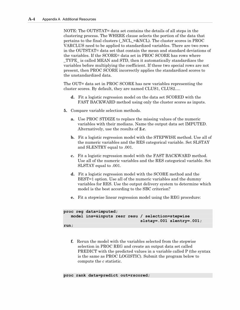
A-4 Appendix A Additional Resources
NOTE: The OUTSTAT= data set contains the details of all steps in the clustering process. The WHERE clause selects the portion of the data that pertains to the final clusters (_NCL_=&NCL). The cluster scores in PROC VARCLUS need to be applied to standardized variables. There are two rows in the OUTSTAT= data set that contain the mean and standard deviations of the variables. If the SCORE= data set in PROC SCORE has rows where _TYPE_ is called MEAN and STD, then it automatically standardizes the variables before multiplying the coefficient. If these two special rows are not present, then PROC SCORE incorrectly applies the standardized scores to the unstandardized data.
The OUT= data set in PROC SCORE has new variables representing the cluster scores. By default, they are named CLUS1, CLUS2….
d. Fit a logistic regression model on the data set SCORED with the FAST BACKWARD method using only the cluster scores as inputs.
5. Compare variable selection methods.
a. Use PROC STDIZE to replace the missing values of the numeric variables with their medians. Name the output data set IMPUTED. Alternatively, use the results of 2.c.
b. Fit a logistic regression model with the STEPWISE method. Use all of the numeric variables and the RES categorical variable. Set SLSTAY and SLENTRY equal to .001.
c. Fit a logistic regression model with the FAST BACKWARD method. Use all of the numeric variables and the RES categorical variable. Set SLSTAY equal to .001.
d. Fit a logistic regression model with the SCORE method and the BEST=1 option. Use all of the numeric variables and the dummy variables for RES. Use the output delivery system to determine which model is the best according to the SBC criterion?
e. Fit a stepwise linear regression model using the REG procedure:
proc reg data=imputed; model ins=&inputs resr resu / selection=stepwise slstay=.001 slentry=.001; run;
f. Rerun the model with the variables selected from the stepwise selection in PROC REG and create an output data set called PREDICT with the predicted values in a variable called P (the syntax is the same as PROC LOGISTIC). Submit the program below to compute the c statistic.
proc rank data=predict out=rscored;

A.1 A1Exercises A-5
var p; run; proc sql; select sum(ins=1) as n1, (sum(p*(ins=1))-.5*(calculated n1)*(calculated n1+1)) /((calculated n1)*(count(ins)-(calculated n1))) as c from rscored; quit;
g. How does the c statistic computed from the model generated in PROC REG compare with the c statistics from the models generated in PROC LOGISTIC?
6. Assess a weighted logistic regression using a validation data set.
a. Split the DEVELOP data set into two data sets. Put 50% of the data into the training data set and 50% into the validation data set. Use a seed of 27513.
b. Fit a weighted model in PROC LOGISTIC using the input variables DDA, DDABAL, DEP, DEPAMT, and CASHBK. Output the parameter estimates to a SAS data set using the OUTEST= option.
c. Score the validation data using the INEST= and MAXITER= options. Create the OUTROC= data set.
d. Create the data set necessary to produce a ROC curve, a lift chart on the top 20% of responders, and an overlay plot of sensitivity, specificity, depth, positive predicted value, and cost ratio in Graph-N-Go. To create a more meaningful graph, select an appropriate range for the cost ratio values.
e. What is the value of LIFT at a 5% depth?
f. What is the cost ratio that optimizes both sensitivity and specificity?
7. Comparing the performance of different models on the validation data set.
a. Use PROC STDIZE to replace the missing values of the numeric variables with their medians. Name the output data set IMPUTED. Alternatively, use the results of 2.c.
b. Split the IMPUTED data set into two data sets. Put 67% of the data into the training data set and 33% into the validation data set. Use a seed of 27513.
c. Fit a logistic regression model with the FAST BACKWARD method. Use all of the numeric variables and the RES categorical variable. Set SLSTAY equal to .0000001.

A-6 Appendix A Additional Resources
d. With the variables selected with the FAST BACKWARD method, rerun the logistic regression model and output the parameter estimates to a SAS data set.
e. Score the validation data set using the INEST= and MAXITER= options. What is the value of the c statistic?
f. Repeat steps c, d, and e, but set SLSTAY equal to .000000001. What is the value of the c statistic on the validation data set?
g. Repeat steps c, d, and e, but set SLSTAY equal to .00000000001. What is the value of the c statistic on the validation data set?
h. Which model had the highest c statistic on the validation data set?

A.2 A2Exercise Solutions A
A.2 A2 Exercise Solutions
1. Score new data using the final parameter estimates from a weighted logistic regression.
data develop; infile 'c:\workshop\winsas\pmlr\ins.dat' missover; input ACCTAGE DDA DDABAL DEP DEPAMT CASHBK CHECKS DIRDEP NSF NSFAMT PHONE TELLER SAV SAVBAL ATM ATMAMT POS POSAMT CD CDBAL IRA IRABAL LOC LOCBAL INV INVBAL ILS ILSBAL MM MMBAL MMCRED MTG MTGBAL CC CCBAL CCPURC SDB INCOME HMOWN LORES HMVAL AGE CRSCORE MOVED INAREA INS BRANCH $ RES $; label ACCTAGE='Age of Oldest Account' DDA='Checking Account' DDABAL='Checking Balance' DEP='Checking Deposits' DEPAMT='Amount Deposited' CASHBK='Number Cash Back' CHECKS='Number of Checks' DIRDEP='Direct Deposit' NSF='Number Insufficient Fund' NSFAMT='Amount NSF' PHONE='Number Telephone Banking' TELLER='Teller Visits' ATM='ATM' ATMAMT='ATM Withdrawal Amount' POS='Number Point of Sale' POSAMT='Amount Point of Sale' CD='Certificate of Deposit' CDBAL='CD Balance' IRA='Retirement Account' IRABAL='IRA Balance' LOC='Line of Credit' LOCBAL='Line of Credit Balance' INV='Investment' INVBAL='Investment Balance' ILS='Installment Loan' ILSBAL='Loan Balance' MM='Money Market' MMBAL='Money Market Balance' MMCRED='Money Market Credits' MTG='Mortgage' MTGBAL='Mortgage Balance' SAV='Saving Account' SAVBAL='Saving Balance' CC='Credit Card' CCBAL='Credit Card Balance'

A-8 Appendix A Additional Resources
CCPURC='Credit Card Purchases' SDB='Safety Deposit Box' INCOME='Income' HMOWN='Owns Home' LORES='Length of Residence' HMVAL='Home Value' AGE='Age' CRSCORE='Credit Score' MOVED='Recent Address Change' INAREA='Local Address' INS='Insurance Product' BRANCH='Branch of Bank' RES='Area Classification'; run; %let inputs=ACCTAGE DDA DDABAL DEP DEPAMT CASHBK CHECKS DIRDEP NSF NSFAMT PHONE TELLER ATM ATMAMT POS POSAMT CD CDBAL IRA IRABAL LOC LOCBAL INV INVBAL ILS ILSBAL MM MMBAL MMCRED MTG MTGBAL SAV SAVBAL CC CCBAL CCPURC SDB INCOME HMOWN LORES HMVAL AGE CRSCORE MOVED INAREA; data new; infile 'c:\workshop\winsas\pmlr\new.dat' missover; input ACCTAGE DDA DDABAL DEP DEPAMT CASHBK CHECKS DIRDEP NSF NSFAMT PHONE TELLER SAV SAVBAL ATM ATMAMT POS POSAMT CD CDBAL IRA IRABAL LOC LOCBAL INV INVBAL ILS ILSBAL MM MMBAL MMCRED MTG MTGBAL CC CCBAL CCPURC SDB INCOME HMOWN LORES HMVAL AGE CRSCORE MOVED INAREA BRANCH $ RES $; label ACCTAGE='Age of Oldest Account' DDA='Checking Account' DDABAL='Checking Balance' DEP='Checking Deposits' DEPAMT='Amount Deposited' CASHBK='Number Cash Back' CHECKS='Number of Checks' DIRDEP='Direct Deposit' NSF='Number Insufficient Fund' NSFAMT='Amount NSF' PHONE='Number Telephone Banking' TELLER='Teller Visits' ATM='ATM' ATMAMT='ATM Withdrawal Amount' POS='Number Point of Sale' POSAMT='Amount Point of Sale' CD='Certificate of Deposit' CDBAL='CD Balance'

A.2 A2Exercise Solutions A
IRA='Retirement Account' IRABAL='IRA Balance' LOC='Line of Credit' LOCBAL='Line of Credit Balance' INV='Investment' INVBAL='Investment Balance' ILS='Installment Loan' ILSBAL='Loan Balance' MM='Money Market' MMBAL='Money Market Balance' MMCRED='Money Market Credits' MTG='Mortgage' MTGBAL='Mortgage Balance' SAV='Saving Account' SAVBAL='Saving Balance' CC='Credit Card' CCBAL='Credit Card Balance' CCPURC='Credit Card Purchases' SDB='Safety Deposit Box' INCOME='Income' HMOWN='Owns Home' LORES='Length of Residence' HMVAL='Home Value' AGE='Age' CRSCORE='Credit Score' MOVED='Recent Address Change' INAREA='Local Address' BRANCH='Branch of Bank' RES='Area Classification'; run; %let pi1=.02; proc means data=develop noprint; var ins; output out=m mean=rho1; run; data m; set m; call symput('rho1',rho1); run; data develop; set develop; sampwt=((1-&pi1)/(1-&rho1))*(ins=0)+(&pi1/&rho1)*(ins=1); run; proc logistic data=develop des outest=betas; weight sampwt; model ins=dda ddabal dep depamt cashbk; run;

A-10 Appendix A Additional Resources
proc score data=new out=scored score=betas type=parms; var dda ddabal dep depamt cashbk; run; data scored; set scored; p=1/(1+exp(-ins)); run; proc print data=scored(obs=25); var p ins dda ddabal dep depamt cashbk; run;
OBS P INS DDA DDABAL DEP DEPAMT CASHBK 1 0.016328 -4.09840 1 56.29 2 955.51 0 2 0.017641 -4.01974 1 3292.17 2 961.60 0 3 0.017053 -4.05423 1 1723.86 2 2108.65 0 4 0.041854 -3.13083 0 0.00 0 0.00 0 5 0.016311 -4.09950 1 67.91 2 519.24 0 6 0.018486 -3.97206 1 2554.58 1 501.36 0 7 0.016404 -4.09367 1 0.00 2 2883.08 0 8 0.016442 -4.09137 1 2641.33 3 4521.61 0 9 0.041854 -3.13083 0 0.00 0 0.00 0 10 0.017392 -4.03422 1 52.22 1 75.59 0 11 0.018988 -3.94477 1 6163.29 2 2603.56 0 12 0.009292 -4.66930 1 431.12 2 568.43 1 13 0.041854 -3.13083 0 0.00 0 0.00 0 14 0.011053 -4.49393 1 112.82 8 2688.75 0 15 0.016199 -4.10650 1 1146.61 3 11224.20 0 16 0.041854 -3.13083 0 0.00 0 0.00 0 17 0.015852 -4.12850 1 1241.38 3 3538.14 0 18 0.018681 -3.96141 1 298.23 0 0.00 0 19 0.016619 -4.08046 1 367.04 2 4242.22 0 20 0.014833 -4.19593 1 1229.47 4 3514.57 0

A.2 A2Exercise Solutions A
21 0.016340 -4.09766 1 37.50 2 1334.17 0 22 0.013643 -4.28082 1 694.92 5 1984.23 0 23 0.005563 -5.18606 1 255.64 1 320.92 2 24 0.016411 -4.09326 1 290.23 2 784.18 0 25 0.012810 -4.34463 1 638.46 6 3448.27 0
data new1; set new; ins1=-3.13082518 -0.83783381*dda + 0.000024303*ddabal – 0.06706434*dep + 0.000003161148*depamt – 0.57878214*cashbk; p=1/(1+exp(-ins1)); run; proc print data=new1(obs=25); var p ins1 dda ddabal dep depamt cashbk; run;
OBS P INS1 DDA DDABAL DEP DEPAMT CASHBK 1 0.016328 -4.09840 1 56.29 2 955.51 0 2 0.017641 -4.01974 1 3292.17 2 961.60 0 3 0.017053 -4.05423 1 1723.86 2 2108.65 0 4 0.041854 -3.13083 0 0.00 0 0.00 0 5 0.016311 -4.09950 1 67.91 2 519.24 0 6 0.018486 -3.97206 1 2554.58 1 501.36 0 7 0.016404 -4.09367 1 0.00 2 2883.08 0 8 0.016442 -4.09137 1 2641.33 3 4521.61 0 9 0.041854 -3.13083 0 0.00 0 0.00 0 10 0.017392 -4.03422 1 52.22 1 75.59 0 11 0.018988 -3.94477 1 6163.29 2 2603.56 0 12 0.009292 -4.66930 1 431.12 2 568.43 1 13 0.041854 -3.13083 0 0.00 0 0.00 0 14 0.011053 -4.49393 1 112.82 8 2688.75 0
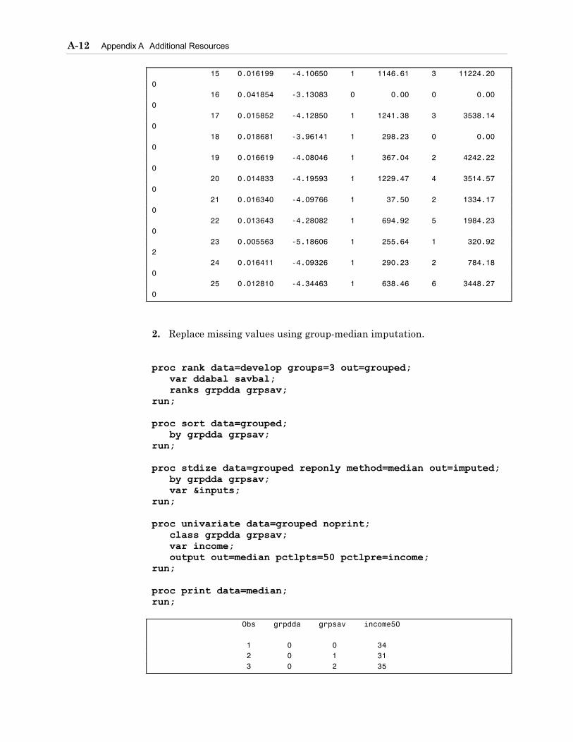
A-12 Appendix A Additional Resources
15 0.016199 -4.10650 1 1146.61 3 11224.20 0 16 0.041854 -3.13083 0 0.00 0 0.00 0 17 0.015852 -4.12850 1 1241.38 3 3538.14 0 18 0.018681 -3.96141 1 298.23 0 0.00 0 19 0.016619 -4.08046 1 367.04 2 4242.22 0 20 0.014833 -4.19593 1 1229.47 4 3514.57 0 21 0.016340 -4.09766 1 37.50 2 1334.17 0 22 0.013643 -4.28082 1 694.92 5 1984.23 0 23 0.005563 -5.18606 1 255.64 1 320.92 2 24 0.016411 -4.09326 1 290.23 2 784.18 0 25 0.012810 -4.34463 1 638.46 6 3448.27 0
2. Replace missing values using group-median imputation.
proc rank data=develop groups=3 out=grouped; var ddabal savbal; ranks grpdda grpsav; run; proc sort data=grouped; by grpdda grpsav; run; proc stdize data=grouped reponly method=median out=imputed; by grpdda grpsav; var &inputs; run; proc univariate data=grouped noprint; class grpdda grpsav; var income; output out=median pctlpts=50 pctlpre=income; run; proc print data=median; run; Obs grpdda grpsav income50 1 0 0 34 2 0 1 31 3 0 2 35

A.2 A2Exercise Solutions A
4 1 0 34 5 1 1 34 6 1 2 35 7 2 0 34 8 2 1 35 9 2 2 35
3. The objective is to cluster the variables and choose a representative one in each cluster.
ods listing close; ods output clusterquality=summary rsquare(match_all)=clusters; proc varclus data=imputed percent=80 outtree=fortree short; var &inputs; run; ods listing; data _null_; set summary; call symput('ncl',trim(left(numberofclusters-2))); run; proc print data=clusters&ncl; run; V R a N S r C O e q i o w x u a n V n t a b t C a C C r l r l r l l e e o u i u o R L l s a s s a a O V t b t e t b b a e l e s i e s r r e r t o l 1 Cluster 1 DEP 0.8057 0.3474 0.2978 Checking Deposits 2 CHECKS 0.8057 0.1543 0.2298 Number of Checks 3 - Cluster 2 MTGBAL 0.9687 0.1976 0.0390 Mortgage Balance 4 CCBAL 0.9687 0.1333 0.0361 Credit Card Balance 5 - Cluster 3 MM 0.9746 0.2963 0.0360 Money Market 6 MMBAL 0.9746 0.2705 0.0348 Money Market Balance 7 - Cluster 4 INCOME 0.8407 0.0265 0.1636 Income 8 HMVAL 0.8407 0.3340 0.2391 Home Value 9 - Cluster 5 ILS 0.9958 0.0393 0.0044 Installment Loan 10 ILSBAL 0.9958 0.0391 0.0044 Loan Balance 11 - Cluster 6 POS 0.9189 0.0711 0.0873 Number Point of Sale 12 POSAMT 0.9189 0.0622 0.0864 Amount Point of Sale

A-14 Appendix A Additional Resources
13 - Cluster 7 HMOWN 0.8156 0.0378 0.1916 Owns Home 14 LORES 0.8156 0.0702 0.1983 Length of Residence 15 - Cluster 8 IRA 1.0000 0.1200 0.0000 Retirement Account 16 - Cluster 9 INVBAL 1.0000 0.0259 0.0000 Investment Balance 17 - Cluster 10 CDBAL 1.0000 0.2028 0.0000 CD Balance 18 - Cluster 11 NSFAMT 1.0000 0.2667 0.0000 Amount NSF 19 - Cluster 12 SDB 1.0000 0.0130 0.0000 Safety Deposit Box 20 - Cluster 13 INAREA 1.0000 0.1159 0.0000 Local Address 21 - Cluster 14 CRSCORE 1.0000 0.1985 0.0000 Credit Score 22 - Cluster 15 LOCBAL 1.0000 0.2212 0.0000 Line of Credit Balance 23 - Cluster 16 CASHBK 1.0000 0.0058 0.0000 Number Cash Back 24 - Cluster 17 SAV 1.0000 0.0640 0.0000 Saving Account 25 - Cluster 18 SAVBAL 1.0000 0.0640 0.0000 Saving Balance 26 - Cluster 19 DEPAMT 1.0000 0.1238 0.0000 Amount Deposited 27 - Cluster 20 DIRDEP 1.0000 0.1298 0.0000 Direct Deposit 28 - Cluster 21 ACCTAGE 1.0000 0.0220 0.0000 Age of Oldest Account 29 - Cluster 22 CCPURC 1.0000 0.1049 0.0000 Credit Card Purchases 30 - Cluster 23 PHONE 1.0000 0.0905 0.0000 Number Telephone Banking 31 - Cluster 24 MOVED 1.0000 0.0016 0.0000 Recent Address Change 32 - Cluster 25 INV 1.0000 0.0459 0.0000 Investment 33 - Cluster 26 TELLER 1.0000 0.1793 0.0000 Teller Visits 34 - Cluster 27 ATMAMT 1.0000 0.0490 0.0000 ATM Withdrawal Amount 35 - Cluster 28 ATM 1.0000 0.1638 0.0000 ATM 36 - Cluster 29 CC 1.0000 0.1049 0.0000 Credit Card 37 - Cluster 30 IRABAL 1.0000 0.1200 0.0000 IRA Balance 38 - Cluster 31 DDABAL 1.0000 0.1238 0.0000 Checking Balance 39 - Cluster 32 DDA 1.0000 0.2993 0.0000 Checking Account 40 - Cluster 33 AGE 1.0000 0.1985 0.0000 Age 41 - Cluster 34 CD 1.0000 0.2028 0.0000 Certificate of Deposit 42 - Cluster 35 LOC 1.0000 0.2212 0.0000 Line of Credit 43 - Cluster 36 MTG 1.0000 0.1692 0.0000 Mortgage 44 - Cluster 37 NSF 1.0000 0.2667 0.0000 Number Insufficient Fund 45 - Cluster 38 MMCRED 1.0000 0.2906 0.0000 Money Market Credits
There were 38 clusters created with the criteria PERCENT=.8.
proc tree data=fortree; height _PROPOR_; run;

A.2 A2Exercise Solutions A
ods listing close; ods output clusterquality=summary rsquare(match_all)=clusters; proc varclus data=imputed maxeigen=.70 outtree=fortree short; var &inputs; run; ods listing; data _null_; set summary; call symput('ncl',trim(left(numberofclusters-2))); run; proc print data=clusters&ncl; run;

A-16 Appendix A Additional Resources
V R a N S r C O e q i o w x u a n V n t a b t C a C C r l r l r l l e e o u i u o R L l s a s s a a O V t b t e t b b a e l e s i e s r r e r t o l 1 Cluster 1 DDA 0.6228 0.1541 0.4460 Checking Account 2 DEP 0.8010 0.2245 0.2566 Checking Deposits 3 CHECKS 0.6441 0.1397 0.4137 Number of Checks 4 - Cluster 2 MTGBAL 0.9687 0.1976 0.0390 Mortgage Balance 5 CCBAL 0.9687 0.1333 0.0361 Credit Card Balance 6 - Cluster 3 MM 0.9138 0.0400 0.0898 Money Market 7 MMBAL 0.8990 0.0325 0.1044 Money Market Balance 8 MMCRED 0.5517 0.0121 0.4538 Money Market Credits 9 - Cluster 4 INCOME 0.8407 0.0206 0.1626 Income 10 HMVAL 0.8407 0.2247 0.2054 Home Value 11 - Cluster 5 ILS 0.9958 0.0446 0.0044 Installment Loan 12 ILSBAL 0.9958 0.0446 0.0044 Loan Balance 13 - Cluster 6 HMOWN 0.8156 0.0327 0.1906 Owns Home 14 LORES 0.8156 0.0489 0.1939 Length of Residence 15 - Cluster 7 POS 0.9189 0.0711 0.0873 Number Point of Sale 16 POSAMT 0.9189 0.0622 0.0864 Amount Point of Sale 17 - Cluster 8 NSF 0.7582 0.0484 0.2541 Number Insufficient Fund 18 NSFAMT 0.7582 0.0339 0.2503 Amount NSF 19 - Cluster 9 CD 0.7252 0.0189 0.2801 Certificate of Deposit 20 CDBAL 0.7252 0.0263 0.2823 CD Balance 21 - Cluster 10 IRA 0.6732 0.0459 0.3426 Retirement Account 22 IRABAL 0.6732 0.0217 0.3341 IRA Balance 23 - Cluster 11 LOC 0.7352 0.0403 0.2759 Line of Credit 24 LOCBAL 0.7352 0.0632 0.2827 Line of Credit Balance 25 - Cluster 12 AGE 0.7228 0.0646 0.2964 Age 26 CRSCORE 0.7228 0.0116 0.2805 Credit Score 27 - Cluster 13 DDABAL 0.6759 0.1083 0.3634 Checking Balance 28 DEPAMT 0.6759 0.0814 0.3528 Amount Deposited 29 - Cluster 14 CC 0.6620 0.0394 0.3519 Credit Card 30 CCPURC 0.6620 0.0538 0.3572 Credit Card Purchases 31 - Cluster 15 INAREA 1.0000 0.0925 0.0000 Local Address 32 - Cluster 16 INVBAL 1.0000 0.0259 0.0000 Investment Balance 33 - Cluster 17 MOVED 1.0000 0.0016 0.0000 Recent Address Change 34 - Cluster 18 SAVBAL 1.0000 0.0640 0.0000 Saving Balance 35 - Cluster 19 CASHBK 1.0000 0.0050 0.0000 Number Cash Back 36 - Cluster 20 SDB 1.0000 0.0123 0.0000 Safety Deposit Box 37 - Cluster 21 ACCTAGE 1.0000 0.0220 0.0000 Age of Oldest Account 38 - Cluster 22 ATMAMT 1.0000 0.0490 0.0000 ATM Withdrawal Amount 39 - Cluster 23 DIRDEP 1.0000 0.1467 0.0000 Direct Deposit 40 - Cluster 24 SAV 1.0000 0.0640 0.0000 Saving Account 41 - Cluster 25 PHONE 1.0000 0.0790 0.0000 Number Telephone Banking 42 - Cluster 26 INV 1.0000 0.0259 0.0000 Investment 43 - Cluster 27 TELLER 1.0000 0.1771 0.0000 Teller Visits

A.2 A2Exercise Solutions A
44 - Cluster 28 ATM 1.0000 0.2052 0.0000 ATM 45 - Cluster 29 MTG 1.0000 0.1692 0.0000 Mortgage
There were 29 clusters created with the criteria MAXEIGEN=.7.
proc tree data=fortree; height _MAXEIG_; run;
ods listing close; ods output clusterquality=summary rsquare(match_all)=clusters; proc varclus data=imputed maxeigen=1 outtree=fortree short; var &inputs; run; ods listing; data _null_; set summary; call symput('ncl',trim(left(numberofclusters-2))); run;
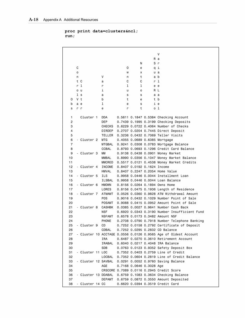
A-18 Appendix A Additional Resources
proc print data=clusters&ncl; run;
V R a N S r C O e q i o w x u a n V n t a b t C a C C r l r l r l l e e o u i u o R L l s a s s a a O V t b t e t b b a e l e s i e s r r e r t o l 1 Cluster 1 DDA 0.5611 0.1847 0.5384 Checking Account 2 DEP 0.7439 0.1995 0.3199 Checking Deposits 3 CHECKS 0.6229 0.0722 0.4064 Number of Checks 4 DIRDEP 0.2707 0.0204 0.7445 Direct Deposit 5 TELLER 0.3236 0.0432 0.7069 Teller Visits 6 - Cluster 2 MTG 0.4055 0.0689 0.6385 Mortgage 7 MTGBAL 0.9241 0.0308 0.0783 Mortgage Balance 8 CCBAL 0.8793 0.0693 0.1296 Credit Card Balance 9 - Cluster 3 MM 0.9138 0.0438 0.0901 Money Market 10 MMBAL 0.8990 0.0356 0.1047 Money Market Balance 11 MMCRED 0.5517 0.0121 0.4538 Money Market Credits 12 - Cluster 4 INCOME 0.8407 0.0192 0.1624 Income 13 HMVAL 0.8407 0.2247 0.2054 Home Value 14 - Cluster 5 ILS 0.9958 0.0446 0.0044 Installment Loan 15 ILSBAL 0.9958 0.0446 0.0044 Loan Balance 16 - Cluster 6 HMOWN 0.8156 0.0264 0.1894 Owns Home 17 LORES 0.8156 0.0475 0.1936 Length of Residence 18 - Cluster 7 ATMAMT 0.0526 0.0360 0.9828 ATM Withdrawal Amount 19 POS 0.9016 0.0432 0.1029 Number Point of Sale 20 POSAMT 0.9088 0.0415 0.0952 Amount Point of Sale 21 - Cluster 8 CASHBK 0.0385 0.0027 0.9641 Number Cash Back 22 NSF 0.6920 0.0343 0.3190 Number Insufficient Fund 23 NSFAMT 0.6578 0.0173 0.3482 Amount NSF 24 PHONE 0.2708 0.0790 0.7918 Number Telephone Banking 25 - Cluster 9 CD 0.7252 0.0158 0.2792 Certificate of Deposit 26 CDBAL 0.7252 0.0295 0.2832 CD Balance 27 - Cluster 10 ACCTAGE 0.0556 0.0126 0.9565 Age of Oldest Account 28 IRA 0.6487 0.0270 0.3610 Retirement Account 29 IRABAL 0.6040 0.0217 0.4048 IRA Balance 30 SDB 0.0763 0.0123 0.9352 Safety Deposit Box 31 - Cluster 11 LOC 0.7352 0.0403 0.2759 Line of Credit 32 LOCBAL 0.7352 0.0604 0.2819 Line of Credit Balance 33 - Cluster 12 SAVBAL 0.0291 0.0052 0.9760 Saving Balance 34 AGE 0.7168 0.0646 0.3028 Age 35 CRSCORE 0.7089 0.0116 0.2945 Credit Score 36 - Cluster 13 DDABAL 0.6759 0.1083 0.3634 Checking Balance 37 DEPAMT 0.6759 0.0872 0.3550 Amount Deposited 38 - Cluster 14 CC 0.6620 0.0394 0.3519 Credit Card

A.2 A2Exercise Solutions A
39 CCPURC 0.6620 0.0295 0.3483 Credit Card Purchases 40 - Cluster 15 ATM 0.5804 0.1490 0.4931 ATM 41 SAV 0.2782 0.0143 0.7323 Saving Account 42 INAREA 0.4842 0.0866 0.5647 Local Address 43 - Cluster 16 INV 0.5804 0.0276 0.4314 Investment 44 INVBAL 0.5804 0.0071 0.4226 Investment Balance 45 - Cluster 17 MOVED 1.0000 0.0006 0.0000 Recent Address Change
There were 17 clusters created with the criteria MAXEIGEN=1.
proc tree data=fortree; height _MAXEIG_; run;
4. Use cluster scores instead of cluster representatives as the input variables in the LOGISTIC procedure .
proc varclus data=imputed maxeigen=.7 outstat=clus noprint; var &inputs; run; data clus; set clus; call symput('ncl',left(_ncl_)); run;

A-20 Appendix A Additional Resources
proc score data=imputed out=scored scores=clus(where=(_ncl_=&ncl or _type_ in ('MEAN','STD'))); var &inputs; run; proc logistic data=scored des; model ins=clus1-clus&ncl / selection=backward fast slstay=.001; run;
Partial Output Summary of Backward Elimination
Effect Number Wald Step Removed DF In Chi-Square Pr > ChiSq 1 Clus12 1 28 0.0033 0.9541 1 Clus8 1 27 0.0796 0.7779 1 Clus23 1 26 0.1881 0.6645 1 Clus16 1 25 0.7615 0.3828 1 Clus2 1 24 0.7629 0.3824 1 Clus17 1 23 0.7787 0.3775 1 Clus7 1 22 0.9021 0.3422 1 Clus15 1 21 1.3663 0.2424 1 Clus20 1 20 6.8397 0.0089 1 Clus6 1 19 8.8215 0.0030 Analysis of Maximum Likelihood Estimates Standard Parameter DF Estimate Error Chi-Square Pr > ChiSq Intercept 1 -0.6691 0.0132 2565.0947 <.0001 Clus1 1 -0.4058 0.0180 506.8141 <.0001 Clus3 1 0.2200 0.0131 282.0981 <.0001 Clus4 1 0.0449 0.0135 10.9911 0.0009 Clus5 1 -0.0585 0.0134 19.0599 <.0001 Clus9 1 0.3406 0.0150 517.6472 <.0001 Clus10 1 0.1018 0.0146 48.6688 <.0001 Clus11 1 -0.0761 0.0143 28.2571 <.0001 Clus13 1 0.3536 0.0234 228.5875 <.0001 Clus14 1 0.1810 0.0138 171.8222 <.0001 Clus18 1 0.6339 0.0304 433.3659 <.0001 Clus19 1 -0.0515 0.0150 11.7622 0.0006 Clus21 1 -0.0884 0.0134 43.6165 <.0001 Clus22 1 0.2225 0.0237 87.9283 <.0001 Clus24 1 0.2472 0.0146 287.3870 <.0001 Clus25 1 -0.0843 0.0166 25.7258 <.0001 Clus26 1 0.1080 0.0129 70.3029 <.0001 Clus27 1 0.1756 0.0148 139.9801 <.0001 Clus28 1 -0.0956 0.0156 37.7642 <.0001 Clus29 1 -0.0802 0.0136 34.6991 <.0001

A.2 A2Exercise Solutions A
Association of Predicted Probabilities and Observed Responses Percent Concordant 76.1 Somers' D 0.524 Percent Discordant 23.6 Gamma 0.526 Percent Tied 0.3 Tau-a 0.237 Pairs 235669575 c 0.762
5. Compare variable selection methods.
proc logistic data=imputed des; class res; model ins=&inputs res / selection=stepwise slstay=.001 slentry=.001; run;
Partial Output Summary of Stepwise Selection
Effect Number Score Wald Step Entered Removed DF In Chi-Square Chi-Square 1 CD 1 1 1324.8994 . 2 SAVBAL 1 2 1069.9853 . 3 MM 1 3 828.2221 . 4 DDABAL 1 4 353.6316 . 5 DDA 1 5 547.6353 . 6 SAV 1 6 324.2678 . 7 CC 1 7 127.1600 . 8 INV 1 8 78.8792 . 9 CHECKS 1 9 70.0239 . 10 TELLER 1 10 98.4344 . 11 ATMAMT 1 11 70.6770 . 12 DEP 1 12 66.6898 . 13 IRA 1 13 55.4320 . 14 ACCTAGE 1 14 48.7831 . 15 LOC 1 15 34.7699 . 16 ATM 1 16 33.0657 . 17 MTG 1 17 25.0278 . 18 PHONE 1 18 23.0845 . 19 ILS 1 19 18.6354 . 20 POSAMT 1 20 15.4641 . 21 POS 1 21 13.8138 .
Summary of Stepwise Selection Step Pr > ChiSq 1 <.0001 2 <.0001 3 <.0001 4 <.0001 5 <.0001

A-22 Appendix A Additional Resources
6 <.0001 7 <.0001 8 <.0001 9 <.0001 10 <.0001 11 <.0001 12 <.0001 13 <.0001 14 <.0001 15 <.0001 16 <.0001 17 <.0001 18 <.0001 19 <.0001 20 <.0001 21 0.0002 Type III Analysis of Effects Wald Effect DF Chi-Square Pr > ChiSq ACCTAGE 1 58.9588 <.0001 DDA 1 179.2871 <.0001 DDABAL 1 332.3891 <.0001 DEP 1 27.4683 <.0001 CHECKS 1 38.5370 <.0001 PHONE 1 23.1182 <.0001 TELLER 1 131.1407 <.0001 ATM 1 33.5606 <.0001 ATMAMT 1 95.7743 <.0001 POS 1 13.7634 0.0002 POSAMT 1 27.7180 <.0001 CD 1 603.6979 <.0001 IRA 1 61.8745 <.0001 LOC 1 23.0512 <.0001 INV 1 59.0649 <.0001 ILS 1 18.3345 <.0001 MM 1 357.7929 <.0001 MTG 1 25.7292 <.0001 SAV 1 276.5300 <.0001 SAVBAL 1 424.4126 <.0001 CC 1 172.3818 <.0001 Analysis of Maximum Likelihood Estimates Standard Parameter DF Estimate Error Chi-Square Pr > ChiSq Intercept 1 -0.7856 0.0389 407.7277 <.0001 ACCTAGE 1 -0.0165 0.00215 58.9588 <.0001 DDA 1 -0.5820 0.0435 179.2871 <.0001 DDABAL 1 0.000058 3.156E-6 332.3891 <.0001 DEP 1 -0.0672 0.0128 27.4683 <.0001 CHECKS 1 -0.0218 0.00351 38.5370 <.0001 PHONE 1 -0.0726 0.0151 23.1182 <.0001

A.2 A2Exercise Solutions A
TELLER 1 0.0748 0.00653 131.1407 <.0001 ATM 1 -0.1906 0.0329 33.5606 <.0001 ATMAMT 1 0.000051 5.16E-6 95.7743 <.0001 POS 1 -0.0377 0.0102 13.7634 0.0002 POSAMT 1 0.00104 0.000198 27.7180 <.0001 CD 1 0.9174 0.0373 603.6979 <.0001 IRA 1 0.4487 0.0570 61.8745 <.0001 LOC 1 -0.2669 0.0556 23.0512 <.0001 INV 1 0.6267 0.0815 59.0649 <.0001 ILS 1 -0.2656 0.0620 18.3345 <.0001 MM 1 0.7679 0.0406 357.7929 <.0001 MTG 1 -0.3121 0.0615 25.7292 <.0001 SAV 1 0.4898 0.0295 276.5300 <.0001 SAVBAL 1 0.000047 2.271E-6 424.4126 <.0001 CC 1 0.3669 0.0279 172.3818 <.0001
Odds Ratio Estimates Point 95% Wald Effect Estimate Confidence Limits ACCTAGE 0.984 0.980 0.988 DDA 0.559 0.513 0.608 DDABAL 1.000 1.000 1.000 DEP 0.935 0.912 0.959 CHECKS 0.978 0.972 0.985 PHONE 0.930 0.903 0.958 TELLER 1.078 1.064 1.092 ATM 0.826 0.775 0.881 ATMAMT 1.000 1.000 1.000 POS 0.963 0.944 0.982 POSAMT 1.001 1.001 1.001 CD 2.503 2.326 2.693 IRA 1.566 1.401 1.752 LOC 0.766 0.687 0.854 INV 1.871 1.595 2.196 ILS 0.767 0.679 0.866 MM 2.155 1.990 2.334 MTG 0.732 0.649 0.826 SAV 1.632 1.540 1.729 SAVBAL 1.000 1.000 1.000 CC 1.443 1.366 1.524 Association of Predicted Probabilities and Observed Responses Percent Concordant 76.4 Somers' D 0.530 Percent Discordant 23.3 Gamma 0.532 Percent Tied 0.3 Tau-a 0.240 Pairs 235669575 c 0.765

A-24 Appendix A Additional Resources
proc logistic data=imputed des; class res; model ins=&inputs res / selection=backward fast slstay=.001; run;
Partial Output Summary of Backward Elimination
Effect Number Wald Step Removed DF In Chi-Square Pr > ChiSq 1 NSF 1 45 0.0065 0.9357 1 AGE 1 44 0.0176 0.8945 1 DIRDEP 1 43 0.1343 0.7140 1 MMCRED 1 42 0.1967 0.6574 1 IRABAL 1 41 0.2269 0.6339 1 CRSCORE 1 40 0.2616 0.6091 1 LORES 1 39 0.5532 0.4570 1 ILSBAL 1 38 0.5991 0.4389 1 INVBAL 1 37 0.6600 0.4166 1 INAREA 1 36 0.7740 0.3790 1 MOVED 1 35 0.8696 0.3511 1 DEPAMT 1 34 0.9391 0.3325 1 NSFAMT 1 33 1.4424 0.2298 1 RES 2 32 3.2862 0.1934 1 CDBAL 1 31 2.1520 0.1424 1 HMOWN 1 30 4.1656 0.0413 1 INCOME 1 29 5.2202 0.0223 1 SDB 1 28 5.2203 0.0223 1 MMBAL 1 27 5.4410 0.0197 1 CCPURC 1 26 5.7554 0.0164 1 MTG 1 25 4.8322 0.0279 1 HMVAL 1 24 8.2437 0.0041 1 CASHBK 1 23 9.8986 0.0017 Type III Analysis of Effects Wald Effect DF Chi-Square Pr > ChiSq ACCTAGE 1 59.9860 <.0001 DDA 1 180.7986 <.0001 DDABAL 1 333.2136 <.0001 DEP 1 28.4122 <.0001 CHECKS 1 38.3809 <.0001 PHONE 1 24.2351 <.0001 TELLER 1 134.4424 <.0001 ATM 1 32.5120 <.0001 ATMAMT 1 101.2251 <.0001 POS 1 13.3693 0.0003 POSAMT 1 25.7886 <.0001 CD 1 604.6382 <.0001 IRA 1 60.8646 <.0001 LOC 1 12.2203 0.0005 LOCBAL 1 17.4424 <.0001

A.2 A2Exercise Solutions A
INV 1 55.2439 <.0001 ILS 1 32.9658 <.0001 MM 1 353.5707 <.0001 MTGBAL 1 45.4754 <.0001 SAV 1 278.1858 <.0001 SAVBAL 1 426.2091 <.0001 CC 1 156.3436 <.0001 CCBAL 1 39.5736 <.0001
Analysis of Maximum Likelihood Estimates Standard Parameter DF Estimate Error Chi-Square Pr > ChiSq Intercept 1 -0.7811 0.0390 402.0139 <.0001 ACCTAGE 1 -0.0166 0.00215 59.9860 <.0001 DDA 1 -0.5849 0.0435 180.7986 <.0001 DDABAL 1 0.000058 3.164E-6 333.2136 <.0001 DEP 1 -0.0684 0.0128 28.4122 <.0001 CHECKS 1 -0.0218 0.00351 38.3809 <.0001 PHONE 1 -0.0745 0.0151 24.2351 <.0001 TELLER 1 0.0759 0.00655 134.4424 <.0001 ATM 1 -0.1878 0.0329 32.5120 <.0001 ATMAMT 1 0.000052 5.197E-6 101.2251 <.0001 POS 1 -0.0371 0.0102 13.3693 0.0003 POSAMT 1 0.00100 0.000198 25.7886 <.0001 CD 1 0.9184 0.0373 604.6382 <.0001 IRA 1 0.4457 0.0571 60.8646 <.0001 LOC 1 -0.2189 0.0626 12.2203 0.0005 LOCBAL 1 -7.95E-6 1.903E-6 17.4424 <.0001 INV 1 0.6067 0.0816 55.2439 <.0001 ILS 1 -0.3712 0.0646 32.9658 <.0001 MM 1 0.7641 0.0406 353.5707 <.0001 MTGBAL 1 -5.21E-6 7.726E-7 45.4754 <.0001 SAV 1 0.4919 0.0295 278.1858 <.0001 SAVBAL 1 0.000047 2.276E-6 426.2091 <.0001 CC 1 0.3469 0.0277 156.3436 <.0001 CCBAL 1 5.095E-6 8.098E-7 39.5736 <.0001

A-26 Appendix A Additional Resources
Odds Ratio Estimates Point 95% Wald Effect Estimate Confidence Limits ACCTAGE 0.984 0.979 0.988 DDA 0.557 0.512 0.607 DDABAL 1.000 1.000 1.000 DEP 0.934 0.911 0.958 CHECKS 0.978 0.972 0.985 PHONE 0.928 0.901 0.956 TELLER 1.079 1.065 1.093 ATM 0.829 0.777 0.884 ATMAMT 1.000 1.000 1.000 POS 0.964 0.945 0.983 POSAMT 1.001 1.001 1.001 CD 2.505 2.328 2.696 IRA 1.562 1.396 1.747 LOC 0.803 0.711 0.908 LOCBAL 1.000 1.000 1.000 INV 1.834 1.563 2.153 ILS 0.690 0.608 0.783 MM 2.147 1.983 2.325 MTGBAL 1.000 1.000 1.000 SAV 1.635 1.544 1.733 SAVBAL 1.000 1.000 1.000 CC 1.415 1.340 1.494 CCBAL 1.000 1.000 1.000 Association of Predicted Probabilities and Observed Responses Percent Concordant 76.5 Somers' D 0.533 Percent Discordant 23.2 Gamma 0.535 Percent Tied 0.3 Tau-a 0.241 Pairs 235669575 c 0.767
data imputed; set imputed; resr=(res='R'); resu=(res='U'); run; ods listing close; ods output modelinfo=model
bestsubsets=score; proc logistic data=imputed des; model ins=&inputs resr resu / selection=score best=1; run; ods listing;
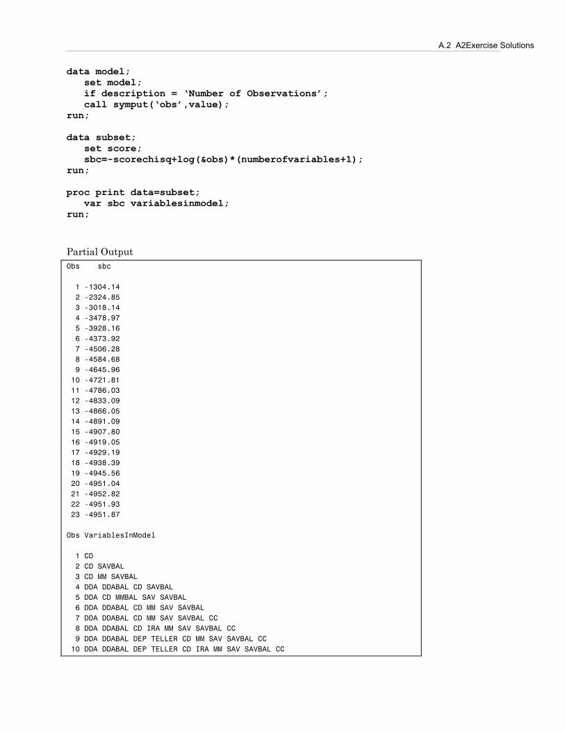
A.2 A2Exercise Solutions A
data model; set model; if description = ‘Number of Observations’; call symput(‘obs’,value); run; data subset; set score; sbc=-scorechisq+log(&obs)*(numberofvariables+1); run; proc print data=subset; var sbc variablesinmodel; run;
Partial Output Obs sbc 1 -1304.14 2 -2324.85 3 -3018.14 4 -3478.97 5 -3928.16 6 -4373.92 7 -4506.28 8 -4584.68 9 -4645.96 10 -4721.81 11 -4786.03 12 -4833.09 13 -4866.05 14 -4891.09 15 -4907.80 16 -4919.05 17 -4929.19 18 -4938.39 19 -4945.56 20 -4951.04 21 -4952.82 22 -4951.93 23 -4951.87 Obs VariablesInModel 1 CD 2 CD SAVBAL 3 CD MM SAVBAL 4 DDA DDABAL CD SAVBAL 5 DDA CD MMBAL SAV SAVBAL 6 DDA DDABAL CD MM SAV SAVBAL 7 DDA DDABAL CD MM SAV SAVBAL CC 8 DDA DDABAL CD IRA MM SAV SAVBAL CC 9 DDA DDABAL DEP TELLER CD MM SAV SAVBAL CC 10 DDA DDABAL DEP TELLER CD IRA MM SAV SAVBAL CC

A-28 Appendix A Additional Resources
11 DDA DDABAL DEP TELLER ATMAMT CD INV MM SAV SAVBAL CC 12 DDA DDABAL DEP TELLER ATMAMT CD IRA INV MM SAV SAVBAL CC 13 ACCTAGE DDA DDABAL DEP TELLER ATMAMT CD IRA INV MM SAV SAVBAL CC 14 ACCTAGE DDA DDABAL DEP TELLER ATMAMT CD IRA LOC INV MM SAV SAVBAL CC 15 ACCTAGE DDA DDABAL DEP PHONE TELLER ATMAMT CD IRA LOC INV MM SAV SAVBAL CC 16 ACCTAGE DDA DDABAL DEP PHONE TELLER ATMAMT CD IRA LOC INV MM MTG SAV SAVBAL CC 17 ACCTAGE DDA DDABAL DEP PHONE TELLER ATM ATMAMT CD IRA LOC INV MM MTG SAV SAVBAL CC 18 ACCTAGE DDA DDABAL DEP PHONE TELLER ATM ATMAMT CD IRA LOC INV ILS MM MTG SAV SAVBAL CC 19 ACCTAGE DDA DDABAL DEP CHECKS PHONE TELLER ATM ATMAMT CD IRA LOC INV ILS MM MTG SAV SAVBAL CC 20 ACCTAGE DDA DDABAL DEP CHECKS PHONE TELLER ATM ATMAMT POSAMT CD IRA LOC INV ILS MM MTG SAV SAVBAL CC 21 ACCTAGE DDA DDABAL DEP CHECKS PHONE TELLER ATM ATMAMT POS POSAMT CD IRA LOC INV ILS MM MTG SAV SAVBAL CC 22 ACCTAGE DDA DDABAL DEP CHECKS PHONE TELLER ATM ATMAMT POS POSAMT CD IRA LOC INV ILS MM MTGBAL SAV SAVBAL CC CCBAL 23 ACCTAGE DDA DDABAL DEP CHECKS PHONE TELLER ATM ATMAMT POS POSAMT CD IRA LOC LOCBAL INV ILS MM MTGBAL SAV SAVBAL CC CCBAL
The 21 variable model had the lowest SBC.
proc reg data=imputed; model ins=&inputs resr resu / selection=stepwise slstay=.001 slentry=.001; run;
Partial Output Summary of Stepwise Selection
Variable Variable Number Partial Model Step Entered Removed Label Vars In R-Square R-Square 1 CD Certificate of Deposit 1 0.0411 0.0411 2 SAVBAL Saving Balance 2 0.0320 0.0730 3 MM Money Market 3 0.0218 0.0948 4 SAV Saving Account 4 0.0134 0.1083 5 DDA Checking Account 5 0.0143 0.1225 6 DDABAL Checking Balance 6 0.0153 0.1378 7 CC Credit Card 7 0.0044 0.1422 8 IRA Retirement Account 8 0.0028 0.1450 9 DEP Checking Deposits 9 0.0021 0.1471 10 TELLER Teller Visits 10 0.0028 0.1499 11 ATMAMT ATM Withdrawal Amount 11 0.0023 0.1522 12 INV Investment 12 0.0018 0.1540 13 ACCTAGE Age of Oldest Account 13 0.0013 0.1553

A.2 A2Exercise Solutions A
14 LOC Line of Credit 14 0.0011 0.1564 Summary of Stepwise Selection Step C(p) F Value Pr > F 1 4644.78 1381.55 <.0001 2 3416.87 1112.22 <.0001 3 2579.52 777.29 <.0001 4 2064.62 485.88 <.0001 5 1517.06 524.97 <.0001 6 931.157 571.53 <.0001 7 762.902 166.36 <.0001 8 658.995 103.81 <.0001 9 580.014 79.57 <.0001 10 474.656 105.84 <.0001 11 388.637 87.00 <.0001 12 321.151 68.83 <.0001 13 271.458 51.28 <.0001 14 231.207 41.97 <.0001 Summary of Stepwise Selection Variable Variable Number Partial Model Step Entered Removed Label Vars In R-Square R-Square 15 PHONE Number Telephone Banking 15 0.0008 0.1573 16 MTG Mortgage 16 0.0007 0.1579 17 ATM ATM 17 0.0006 0.1586 18 ILS Installment Loan 18 0.0006 0.1592 19 CHECKS Number of Checks 19 0.0005 0.1597 20 POSAMT Amount Point of Sale 20 0.0005 0.1602 21 POS Number Point of Sale 21 0.0004 0.1606 22 CASHBK Number Cash Back 22 0.0003 0.1609 Summary of Stepwise Selection Step C(p) F Value Pr > F 15 200.887 32.14 <.0001 16 177.078 25.68 <.0001 17 154.604 24.37 <.0001 18 133.247 23.27 <.0001 19 114.314 20.87 <.0001 20 97.3936 18.88 <.0001 21 84.8851 14.48 0.0001 22 75.9591 10.91 0.0010 proc reg data=imputed noprint; model ins= CD SAVBAL MM SAV DDA DDABAL CC IRA DEP TELLER ATMAMT INV ACCTAGE LOC PHONE MTG ATM ILS CHECKS

A-30 Appendix A Additional Resources
POSAMT POS CASHBK; output out=predict p=p; run; proc rank data=predict out=rscored; var p; run; proc sql; select sum(ins=1) as n1, (sum(p*(ins=1))-.5*(calculated n1)*(calculated n1+1)) /((calculated n1)*(count(ins)-(calculated n1))) as c from rscored; quit; n1 c ƒƒƒƒƒƒƒƒƒƒƒƒƒƒƒƒƒƒ 11175 0.752557
The c statistic from the model generated in the REG procedure is lower than the models generated in PROC LOGISTIC.
6. Assess a weighted logistic regression using a validation data set. data train validate; set develop; u=ranuni(27513); if u<=.50 then output train; else output validate; run; proc logistic data=train des outest=betas; weight sampwt; model ins = dda ddabal dep depamt cashbk; run; proc logistic data=validate des inest=betas; model ins=dda ddabal dep depamt cashbk / maxiter=0 outroc=roc; run; data roc; set roc; cutoff=_PROB_; specif=1-_1MSPEC_; tp=&pi1*_SENSIT_; fn=&pi1*(1-_SENSIT_); tn=(1-&pi1)*specif;

A.2 A2Exercise Solutions A
fp=(1-&pi1)*_1MSPEC_; depth=tp+fp; pospv=tp/depth; negpv=tn/(1-depth); acc=tp+tn; lift=pospv/&pi1; keep cutoff tn fp fn tp _SENSIT_ _1MSPEC_ specif depth pospv negpv acc lift; run;
data roc1; set roc; if .001<depth<.2; run;

A-32 Appendix A Additional Resources
The lift value at a 5% depth is approximately 3.35.
data roc2; set roc; costrat=int((1-cutoff)/cutoff); if costrat ge 40 and costrat le 70; run;

A.2 A2Exercise Solutions A
The cost ratio that optimizes both sensitivity and specificity is 57.
7. Comparing the performance of different models on the validation data set.
data train validate; set imputed; u=ranuni(27513); if u<=.67 then output train; else output validate; run; proc logistic data=train des; class res; model ins = &inputs res / selection=backward fast slstay=.0000001; run;

A-34 Appendix A Additional Resources
Partial Output Analysis of Maximum Likelihood Estimates
Standard Parameter DF Estimate Error Chi-Square Pr > ChiSq Intercept 1 -0.8619 0.0461 349.7584 <.0001 ACCTAGE 1 -0.0163 0.00262 38.9648 <.0001 DDA 1 -0.6014 0.0524 131.9709 <.0001 DDABAL 1 0.000056 3.798E-6 220.5494 <.0001 DEP 1 -0.1320 0.0134 97.2527 <.0001 TELLER 1 0.0731 0.00774 89.1512 <.0001 ATMAMT 1 0.000044 5.876E-6 55.5262 <.0001 CD 1 0.9311 0.0454 420.2910 <.0001 IRA 1 0.4495 0.0690 42.4711 <.0001 LOCBAL 1 -0.00001 2.226E-6 39.1086 <.0001 INV 1 0.6580 0.0995 43.7641 <.0001 ILSBAL 1 -0.00004 7.432E-6 32.5641 <.0001 MM 1 0.7482 0.0493 230.2008 <.0001 MTGBAL 1 -6.79E-6 1.034E-6 43.1183 <.0001 SAV 1 0.5023 0.0356 199.5740 <.0001 SAVBAL 1 0.000047 2.757E-6 289.9243 <.0001 CC 1 0.3617 0.0331 119.1024 <.0001 CCBAL 1 6.616E-6 1.094E-6 36.6033 <.0001 proc logistic data=train des outest=betas; model ins = ACCTAGE DDA DDABAL DEP TELLER ATMAMT CD IRA LOCBAL INV ILSBAL MM MTGBAL SAV SAVBAL CC CCBAL; run; proc logistic data=validate des inest=betas; model ins= ACCTAGE DDA DDABAL DEP TELLER ATMAMT CD IRA LOCBAL INV ILSBAL MM MTGBAL SAV SAVBAL CC CCBAL / maxiter=0; run;
Partial Output Association of Predicted Probabilities and Observed Responses
Percent Concordant 76.3 Somers' D 0.530 Percent Discordant 23.4 Gamma 0.531 Percent Tied 0.3 Tau-a 0.241 Pairs 25977438 c 0.765
proc logistic data=train des; class res; model ins = &inputs res / selection=backward fast slstay=.000000001; run;

A.2 A2Exercise Solutions A
Partial Output Analysis of Maximum Likelihood Estimates
Standard Parameter DF Estimate Error Chi-Square Pr > ChiSq Intercept 1 -0.8728 0.0459 361.7448 <.0001 ACCTAGE 1 -0.0163 0.00261 39.2949 <.0001 DDA 1 -0.5861 0.0522 126.1634 <.0001 DDABAL 1 0.000056 3.792E-6 217.0620 <.0001 DEP 1 -0.1310 0.0133 96.2986 <.0001 TELLER 1 0.0685 0.00769 79.3993 <.0001 ATMAMT 1 0.000038 5.727E-6 43.7508 <.0001 CD 1 0.9385 0.0453 429.5670 <.0001 IRA 1 0.4454 0.0687 42.0291 <.0001 INV 1 0.6595 0.0990 44.3862 <.0001 MM 1 0.7397 0.0491 227.0297 <.0001 SAV 1 0.5025 0.0354 201.2822 <.0001 SAVBAL 1 0.000047 2.735E-6 291.6220 <.0001 CC 1 0.3183 0.0323 96.8727 <.0001
proc logistic data=train des outest=betas; model ins = ACCTAGE DDA DDABAL DEP TELLER ATMAMT CD IRA INV MM SAV SAVBAL CC; run; proc logistic data=validate des inest=betas; model ins= ACCTAGE DDA DDABAL DEP TELLER ATMAMT CD IRA INV MM SAV SAVBAL CC / maxiter=0; run;
Partial Output Association of Predicted Probabilities and Observed Responses
Percent Concordant 76.2 Somers' D 0.528 Percent Discordant 23.5 Gamma 0.530 Percent Tied 0.3 Tau-a 0.240 Pairs 25977438 c 0.764
proc logistic data=train des; class res; model ins = &inputs res / selection=backward fast slstay=.00000000001; run;

A-36 Appendix A Additional Resources
Partial Output Analysis of Maximum Likelihood Estimates
Standard Parameter DF Estimate Error Chi-Square Pr > ChiSq Intercept 1 -0.9370 0.0435 464.2778 <.0001 DDA 1 -0.6132 0.0517 140.8948 <.0001 DDABAL 1 0.000058 3.772E-6 233.5893 <.0001 DEP 1 -0.1051 0.0126 69.3555 <.0001 TELLER 1 0.0590 0.00754 61.1813 <.0001 CD 1 0.9397 0.0451 433.3906 <.0001 INV 1 0.7339 0.0971 57.1517 <.0001 MM 1 0.7523 0.0486 239.2955 <.0001 SAV 1 0.5240 0.0353 220.6467 <.0001 SAVBAL 1 0.000048 2.735E-6 313.8942 <.0001 CC 1 0.3167 0.0320 97.9412 <.0001
proc logistic data=train des outest=betas; model ins = DDA DDABAL DEP TELLER CD INV MM SAV SAVBAL CC; run; proc logistic data=validate des inest=betas; model ins= DDA DDABAL DEP TELLER CD INV MM SAV SAVBAL CC / maxiter=0; run;
Partial Output Association of Predicted Probabilities and Observed Responses
Percent Concordant 75.6 Somers' D 0.517 Percent Discordant 23.9 Gamma 0.519 Percent Tied 0.5 Tau-a 0.235 Pairs 25977438 c 0.758
The seventeen-variable model had the highest c statistic on the validation data set (.765).

A.3 A3References A-37
A.3 A3 References
Breiman, L., Friedman, J. H., Olshen, R. A., and Stone, C. J. (1984), Classification and Regression Trees, Chapman and Hall.
Cohen, A. (1991), “Dummy Variables in Stepwise Regression,” The American Statistician, 45, 226-228.
Conover, W. J. (1980), Practical Nonparametric Statistics, New York: John Wiley & Sons.
Donner, A. (1982), “The Relative Effectiveness of Procedures Commonly Used in Multiple Regression Analysis for Dealing with Missing Values,” The American Statistician, 36, 378-381.
Duffy, T. J. and Santner, D. E. (1989), The Statistical Analysis of Discrete Data, New York: Springer-Verlag.
Greenacre, M. J. (1988), “Clustering Rows and Columns of a Contingency Table,” Journal of Classification, 5, 39-51.
Greenacre, M. J. (1993), Correspondence Analysis in Practice, San Diego, CA: Academic Press.
Hand, D. J. (1997), Construction and Assessment of Classification Rules, New York: John Wiley & Sons.
Hand, D. J. and Henley, W. E. (1997), “Statistical Classification Methods in Consumer Credit Scoring: A Review,” Journal of the Royal Statistical Society A, 160, 153-541.
Harrell, F. E. (1997), Predicting Outcomes: Applied Survival Analysis and Logistic Regression, Charlottesville Virginia: School of Medicine, University of Virginia.
Hastie, T. J. and Tibshirani, R. J. (1990), Generalized Additive Models, London: Chapman and Hall.
Huber, P. J. (1997), “From Large to Huge: A Statistician’s Reactions to KDD & DM,” Proceedings of the Third International Conference on Knowledge Discovery and Data Mining, Menlo Park, CA: AAAI Press.
Jackson, J. E. (1991), A Users Guide to Principal Components, New York: John Wiley & Sons.
Jones, M. P. (1996), “Indicator and Stratification Methods for Missing Explanatory Variables in Multiple Linear Regression,” Journal of the American Statistical Association, 91, 222-230.
Lawless, J. F. and Singhal, K. (1978), “Efficient Screening of Nonnormal Regression Models,” Biometrics, 34, 318-327.

A-38 Appendix A Additional Resources
Little, R. J. A. (1992), “Regression with Missing X’s: A Review,” Journal of the American Statistical Association, 87, 1227-1237.
Mantel, N. (1970), “Why Stepdown Procedures in Variable Selection,” Technometrics, 12, 621-625.
Magee, L. (1998), “Nonlocal Behavior in Polynomial Regressions,” The American Statistician, 52, 20-22.
McLachlan, G. J. (1992), Discriminant Analysis and Statistical Pattern Recognition, New York: John Wiley & Sons.
Nelson, R. W. (1997), Credit Card Risk Management, Warren Taylor Publications.
Prentice, R. L. and Pike, R. (1979), “Logistic Disease Incidence Models and Case-Control Studies,” Biometrika, 66, 403-411.
Ripley, B. D. (1996), Pattern Recognition and Neural Networks, Cambridge University Press.
Sarle, W. S. (1994), “Neural Networks and Statistical Models,” Proceedings of the 19th Annual SUGI, Cary, NC: SAS Institute Inc.
SAS Institute Inc., SAS Language: Reference, Version 6, First Edition, Cary, NC: SAS Institute Inc., 1990.
SAS Institute Inc., SAS Procedures Guide, Version 6, Third Edition, Cary, NC: SAS Institute Inc., 1990.
SAS Institute Inc., SAS/STAT Users Guide, Version 6, Fourth Edition, Volume 1, Cary, NC: SAS Institute Inc., 1990.
SAS Institute Inc., SAS/STAT Users Guide, Version 6, Fourth Edition, Volume 2, Cary, NC: SAS Institute Inc., 1990.
SAS Institute Inc., Logistic Regression Examples Using the SAS System, Version 6, First Edition, Cary, NC: SAS Institute Inc., 1995.
SAS Institute Inc., SAS/STAT Software: Changes and Enhancements through Release 6.12, Cary, NC: SAS Institute Inc., 1997.
Scott, A. J. and Wild, C. J. (1986), “Fitting Logistic Regression Models under Case-Control or Choice Based Sampling, ” Journal of the Royal Statistical Society B, 48, 170-182.
Scott, A. J. and Wild, C. J. (1997), “Fitting Regression Models to Case-Control Data by Maximum Likelihood,” Biometrika, 84, 57-71.

Appendix B Index
% %LET statement, 1-5
A accuracy, 4-17 activation function, 5-14 adding cost ratios, 4-35 attrition predicting, 1-4
B backward elimination method, 3-44 Bayes rule, 4-32 binary indicator variables, 2-2 binary logistic regression model, 2-8–2-12 binary target, 5-15 bins, 5-3
C c statistic, 4-38, 4-40 calculating misclassification measures, 4-23–4-
29 cases, 1-2 categorical inputs, 3-10 class separation, 4-36 CLASS statement, LOGISTIC procedure
PARAM option, 2-8 REF option, 2-8
CLASS statement, MEANS procedure, 5-4 classification rules
depth, 4-20 cluster components, 3-23 cluster imputation, 3-9 CLUSTER procedure
FREQ statement, 3-14 cluster representatives, 3-26 clustering levels, 3-12, 3-14–3-20 cluster-mean imputation, 3-9 coefficients, 3-24 complete-case analysis, 3-3 concentration curves, 4-20 confusion matrix, 4-17, 4-30 cost ratios, 4-34
adding, 4-35 creating missing indicators, 3-6–3-8 credit scoring, 1-4 cross-validation, 4-4 cubic models, 5-8 curse of dimensionality, 1-11, 5-2, 5-10 cutoff values, 4-30
D data set
test, 4-3 training, 4-3 validation, 4-3
data splitting, 4-3, 4-5–4-16 database marketing, 1-4 decision trees, 5-17 degree, 5-8 depth
classification rules, 4-20 DES option
PROC LOGISTIC statement, 2-8 dimensions, 1-11, 5-2 divergence statistics, 4-36 divisive clustering, 3-25 dummy variables, 3-10
E EDF option
PROC NPAR1WAY statement, 4-39 eigenvalues, 3-22 eigenvectors, 3-24 empirical logits, 5-3
plotting, 5-4–5-6 Enterprise Miner, 5-17 equivalent kernel, 5-10 error rate, 4-17 estimators
flexible multivariate function, 5-7
F FAST option
MODEL statement (LOGISTIC), 3-46 feed-forward neural networks, 5-14 fitted surface, 2-4 fitting a neural network, 5-17–5-18 flexibility, 5-16 flexible multivariate function estimators, 5-7 forward selection method, 3-44, 5-11 fraud detection, 1-4 FREQ procedure, 1-5 FREQ statement
CLUSTER procedure, 3-14
G gains charts, 4-20 generalization, 1-3 generalized linear model, 2-3 Graph-N-Go application, 4-27

B-2 Index
Greenacre’s method, 3-14 GROUPS= option
PROC RANK statement, 5-4
H H= option
PROC TREE statement, 3-19 hand-crafted
input variables, 5-7 HEIGHT statement
TREE procedure, 3-34 HI option
PROC VARCLUS statement, 3-27 hidden layers, 5-14 hidden units, 5-14 high dimensionality, 1-11 higher degree polynomials, 5-8 HOEFFDING option
PROC CORR statement, 3-37 Hoeffding’s D statistics, 3-37
I imputation
indicators, 3-5 missing values, 3-4
INCLUDE= option MODEL statement (LOGISTIC), 5-11
incomprehensibility, 5-14 indicators
imputation, 3-5 INEST= option
PROC LOGISTIC statement, 4-23 input layers, 5-14 input variables, 1-2
binning, 5-4 hand-crafted, 5-7 transforming, 5-7
interactions, 1-13, 5-2 ITPRINT option
MODEL statement (LOGISTIC), 2-8
J joint sampling, 2-16
K Kolmogorov-Smirnov test statistics (K-S), 4-
37, 4-39
L lift charts, 4-20 LISTING statement
Output Delivery System (ODS), 3-13 logistic discrimination, 2-6 LOGISTIC procedure
CLASS statement, 2-8 MODEL statement, 2-8
scalability, 3-45 UNITS statement, 2-8 WEIGHT statement, 2-24
logistic regression model, 5-7 binary, 2-8–2-12
logit link function, 2-3 Lorentz curves, 4-20
M MAXEIGEN= option
PROC VARCLUS statement, 3-27 maximum likelihood estimates, 2-7 MAXITER= option
MODEL statement (LOGISTIC), 4-23 mean-imputation, 3-9 MEANS procedure, 1-5
CLASS statement, 5-4 OUTPUT statement, 2-19, 5-4
measurement scales, 1-10 METHOD= option
PROC CLUSTER statement, 3-14 PROC STDIZE statement, 3-7
MINID option OUTPUT statement (MEANS), 3-18
misclassification costs, 4-31 misclassification measures
calculating, 4-23–4-29 missing completely at random (MCAR), 3-2 missing indicators, 3-6–3-8 missing values, 3-2
imputation, 3-4 model interpretation, 2-5 model selection
overfitting, 1-13 underfitting, 1-13
MODEL statement, LOGISITC procedure FAST option, 3-46 SELECTION= option, 3-46 SLSTAY option, 3-47
MODEL statement, LOGISTIC procedure INCLUDE= option, 5-11 ITPRINT option, 2-8 MAXITER= option, 4-23 OFFSET= option, 2-20, 4-23 OUTROC= option, 4-23 ROCEPS = option, 4-26 STB option, 2-8
multilayer perceptron (MLP), 5-15 multivariate relationships, 5-2
N NCLUSTERS= option
PROC TREE statement, 3-19 neural networks
artificial, 5-14 feed-forward, 5-14 fitting, 5-17–5-18
nonlinear regression models, 5-14 nonlinear transformations, 5-15 nonlinearities, 1-13, 5-2, 5-7

Index B-3
non-local behavior, 5-10 number of terms, 5-10 NWAY option
PROC MEANS statement, 3-14
O OFFSET option
MODEL statement (LOGISTIC), 2-20 OFFSET= option
MODEL statement (LOGISTIC), 4-23 offsets, 2-17–2-18 opportunistic data, 1-9 OUT= option
PROC SCORE statement, 2-14 PROC STDIZE statement, 3-7
OUTEST= option PROC LOGISTIC statement, 2-14
output activation function, 5-14 Output Delivery System (ODS), 3-13
LISTING statement, 3-13 OUTPUT statement, 3-13, 3-32 TRACE statement, 3-13
output layers, 5-14 OUTPUT statement, MEANS procedure, 2-19,
5-4 MINID option, 3-18
OUTPUT statement, Output Delivery System (ODS), 3-13, 3-32
OUTPUT statement, UNIVARIATE procedure PCTLPRE option, 4-16 PCTLPTS option, 4-16
OUTREE= option PROC VARCLUS statement, 3-27
OUTROC= option MODEL statement (LOGISTIC), 4-23
OUTTREE= option PROC CLUSTER statement, 3-14
overfitting, 4-2 model selection, 1-13
oversampled test set, 4-21 oversampling, 2-17
adjustments, 4-22
P PARAM option
CLASS statement (LOGISTIC), 2-8 PCTLPRE option
OUTPUT statement (UNIVARIATE), 4-16 PCTLPTS option
OUTPUT statement (UNIVARIATE), 4-16 plotting empirical logits, 5-4–5-6 polynomial models, 5-7, 5-9 polynomials
higher degree, 5-8 posterior probability, 2-2, 2-18 predicted values, 4-18 predictive model, 1-2
business applications, 1-4 principal components analysis, 3-22 prior probabilities, 4-22
priors, 2-16 PROC CLUSTER statement
METHOD= option, 3-14 OUTTREE= option, 3-14
PROC CORR statement HOEFFDING option, 3-37 RANK option, 3-37 SPEARMAN option, 3-37
PROC LOGISTIC statement DES option, 2-8 INEST= option, 4-23 OUTEST= option, 2-14
PROC MEANS statement NWAY option, 3-14
PROC NPAR1WAY statement EDF option, 4-39 WILCOXON option, 4-39
PROC RANK statement GROUPS= option, 5-4
PROC SCORE statement OUT= option, 2-14 TYPE= option, 2-14
PROC STDIZE statement METHOD= option, 3-7 OUT= option, 3-7 REPONLY option, 3-7
PROC TREE statement H= option, 3-19 NCLUSTERS= option, 3-19
PROC VARCLUS statement HI= option, 3-27 MAXEIGEN= option, 3-27 OUTREE= option, 3-27 SHORT option, 3-27
Q quadratic models, 5-8 quasi-complete separation, 3-11
R RANK option
PROC CORR statement, 3-37 RANK procedure
RANKS statement, 5-4 VAR statement, 5-4
RANKS statement RANK procedure, 5-4
RANUNI function, 4-6 rare target event, 1-12 receiver operating characteristic (ROC), 4-19
area under the curve, 4-38 redundancy, 3-21 REF option
CLASS statement (LOGISTIC), 2-8 REPONLY option
PROC STDIZE statement, 3-7 retail banking example, 1-5–1-8 ROC curve, 4-38 ROCEPS = option
MODEL statement (LOGISTIC), 4-26

B-4 Index
S sampling
joint, 2-16 separate, 2-16
sampling weights, 2-23–2-26 scalability
LOGISTIC procedure, 3-45 scatter plots, 5-2 Schwarz Bayes criterion (SBC), 3-49 scorability, 3-4 SCORE procedure
VAR statement, 2-14 scoring new cases, 2-13 selecting subsets, 3-47–3-51 SELECTION= option
MODEL statement (LOGISTIC), 3-46 sensitivity, 4-18 separate sampling, 2-16, 2-19–2-22 SHORT option
PROC VARCLUS statement, 3-27 sigmoidal surface, 5-16 skip layers, 5-14 SLSTAY option
MODEL statement (LOGISTIC), 3-47 Spearman correlation statistics, 3-37 SPEARMAN option
PROC CORR statement, 3-37 specificity, 4-18 STB option
MODEL statement (LOGISTIC), 2-8 STDIZE procedure
VAR statement, 3-7 stepwise selection method, 3-43 subsets selection, 3-42, 3-47–3-51 supervised classification, 1-2 SYMPUT routine, 2-19, 3-32
T target marketing, 1-4
target variables, 1-2 terms, 5-9 test data set, 4-3 TRACE statement
Output Delivery System (ODS), 3-13 training data set, 4-3 transforming
input variables, 5-7 TREE procedure
HEIGHT statement, 3-34 TYPE= option
PROC SCORE statement, 2-14
U underfitting
model selection, 1-13 UNITS statement
LOGISTIC procedure, 2-8 univariate screening, 3-36–3-41 univariate smoothing, 5-2 universal approximators, 5-14
V validation data set, 4-3 VAR statement, RANK procedure, 5-4 VAR statement, SCORE procedure, 2-14 VAR statement, STDIZE procedure, 3-7 VAR statement, VARCLUS procedure, 3-27 VARCLUS procedure
VAR statement, 3-27 variable clustering, 3-27–3-35
W WEIGHT statement
LOGISTIC procedure, 2-24 WILCOXON option
PROC NPAR1WAY statement, 4-39 Wilcoxon test statistics, 4-39

Index B-5

B-6 Index