Predictive Modelling Of Household Energy Demand · Predictive Modelling of Household Energy Demand Said Sabir dpw1013f18 With economic growth and huge increase in the population,

1

Predictive Modelling Of Household

Energy Demand

Aalborg University

Department of Computer Science

Database and Programming Technologies

Project Report

Said Sabir

dpw1013f18

2

Department of Computer Science Aalborg University http://www.aau.dk

Abstract:

Project Period:

Fall Semester 2018

Project Group:

dpw1013f18

Participant(s):

Said Sabir

[email protected]

Supervisor(s):

Bijay Neupane

Copies: 1

Number of pages: 60

Date of Completion:

June 15, 2018

The content of this report is freely available, but publication (with reference) may only be pursued due to an agreement with

the author

In the energy domain, accurate forecasts of electricity

demand and supply are a fundamental prerequisite for

balancing electric power consumption and

production and thus, for the stability and reliability of

the electricity grids.

One of the most promising approaches to

confronting this challenge is utilizing energy demand

flexibility from household devices to maintain energy

balance dynamically. The flexibility refers to the

possibility of preponing or postponing a portion of

electrical demands from households to align the

supply and demand.

In this project, we try performing a comprehensive

data analysis of household energy consumption

patterns and the grouping of similar households.

Henceforth, design a household-level prediction

model that utilize historical energy consumption data

and contextual information to predict future device

activation and associated energy demand.

http://www.aau.dk/

3

Contents

Research summary................................................................................................................... 5

Chapter 1 Research Summary .................................................................................................................... 5

Predictive Modelling of Household Energy Demand ............................................................ 5

Chapter 1 .................................................................................................................................. 7

1.1 Introduction .................................................................................................................... 7

Chapter 2 ................................................................................................................................ 12

Chapter 3 ................................................................................................................................ 19

3.1 Dataset................................................................................................................................ 19

3.2 Problem Formulation ..................................................................................................... 19

Chapter 4 ................................................................................................................................ 21

Background ........................................................................................................................ 21

Chapter 5 ................................................................................................................................ 29

5.1 Data analysis methodology .......................................................................................... 29

5.2 Trend and Seasonality ................................................................................................. 31

5.3 Aggregation-level-dependent-Predictability .............................................................. 31

5.4 Clustering...................................................................................................................... 31

Figure 5.3: Schematic representation of the procedure for clustering ................................. 32

5.5 Forecasting.................................................................................................................... 32

5.6 Time Series Context and Context drifts..................................................................... 34

Chapter 6 ................................................................................................................................ 35

6.1 Analysis ......................................................................................................................... 35

6.2 Data Manipulation/Engineering ................................................................................. 36

6.3 Clustering of household energy consumption ........................................................... 38

6.4 Data preparation for forecasting ................................................................................ 41

4

6.5 Models used for forecasting ........................................................................................ 41

6.6 Evaluation ..................................................................................................................... 43

Chapter 7 ............................................................................................................................ 51

7.1 Discussion...................................................................................................................... 51

7.2 Conclusion .................................................................................................................... 52

5

Research Summary

Predictive Modelling of Household Energy Demand

Said Sabir

dpw1013f18

With economic growth and huge increase in the population, the consumption of energy

has increased multi-fold in the recent years. Such as for an instance, in China, electricity

consumption accounted for 28% of the total energy consumption in 2011, and that it will reach

35% by 2020 [1] and in the US, electricity consumption is close to 39% of the total energy

consumption [2] and it is increasing every year. We are in a great demand of electricity and we

are also utilising it to an extreme end. Therefore, it is quite important to build an efficient

system to monitor, control and optimise the energy utilization rate for making good decisions

to control the supply and usage of various electric equipment and is very important for the

reliable and efficient operation of power systems and as well as money saving.

The domain of electricity load forecasting is quite mature where numerous approaches

have been proposed and tried upon throughout the years. Most of these, usually focused on

system level demand forecasting, with a load reaching tens of megawatts or gigawatts. A

simple overview of a short-term load forecasting approach can be found in [3-4], and some

more classic surveys are provided in [5] and [6]. There are different methods that have been

proposed for forecasting the electric load demand in the last few decades. Among them, some

of the most popular are time series analyses with the autoregressive integrated moving average

or (ARIMA) method [7], the fuzzy logic method [8], the neuro-fuzzy method [9], artificial

neural networks (ANNs), and support vector machines (SVMs).

The main objective of the research is to build a new and more effective, robust, reliable

and efficient prediction models to forecast the energy needs for next 24 hours based on the

previous dataset on the individual household level and to understand what extent if it is viable.

We can later on, predict the energy demands for a much longer duration such as a week, month

or a quarter etc. The dataset consists of energy consumption profiles for 58 different houses,

each containing patterns of 3 to 9 individual devices logged at a frequency of once every 2

6

minutes when idle and 2-8 seconds when in use. The dataset was collected for the duration of

6 months to 1 year from households in Denmark and Italy. Further, the dataset consists of

power demand profile that was annotated with various context values such as family size

ranging from 1-5 adults per house, house area ranging from 80-700m2, etc.

The model utilities fuzzy c means clustering to cluster the households based on their

energy demands and predict the needs of all of the households using a different kind of

forecasting models such as HoltWinters, ARIMA, ETS and Snaive model for identifying

patterns of household behavior in terms of consumption of energy and comparing the models

w.r.t. error (MAE, MAPE, MaxAE & Sigma) to find the best model. The error in forecasting

of Holt-Winter's model result least error in 4 of the clusters and a very competitive error in rest

of the clusters. Also, considering the seasonal behavior of energy consumption and error in the

result Holt-Winter's model was quite effective. We were able to achieve up to 93.35% accuracy

for some of the clusters using exponential smoothening methods like Holt-Winters and ETS

models.

We Identified similar houses based on their energy consumption profile and cluster

them together. Now for the new house we will just need to identify the exact cluster it belongs,

and more accurate forecasting could be done in a very less amount of time. There are also some

challenges in forecasting of a load of an individual household level due to its extreme system

volatility which arises as a result of dynamic processes composed of numerous individual

components and various usage at different household, but a more advanced clustering

technique can help us to attain better results in this case. The research can further be extended

to apply energy prediction model to build a Building Energy Management System (BEMS) and

establish databases and collect precise and sufficient historical consumption data from various

cases for further research use to achieve mutual benefits and save energy and money. Artificial

intelligence models can be used instead of traditional models such as ARIMA with proper

optimizations of parameters for accurate prediction.

7

Chapter 1

1.1 Introduction

Across the European Union, there has been significant interest for smarter electricity

networks, where more significant control over the supply of electricity and its consumption

is going to be achieved as a result of investments and improvements in new technologies such

as Advanced Metering Infrastructure (AMI). Smart metering is a part of this movement, and

it is expected to be crucial in achieving the EU energy policy goals by the year 2020, in other

words, to cut the greenhouse gas emissions by 20%, to help improve energy efficiency by

20% and to ensure that 20% of the energy demand of the European Union is supplied through

renewable energy sources.

Such Smart metering systems are a kind of micro-grid systems which includes different types

of operational and energy-based measures like renewable energy resources, smart appliances,

and energy efficient resources. One of the biggest challenges associated with the operation of

such micro-grids is the optimal energy management of residential buildings concerning

multiple and often conflicting objectives [10]. In recent days, considerable attention is paid

to smart grid vision and smarter homes having the ability to optimize energy consumption

and thus generating lower electricity bills. Thus, developing a smart home energy

management system is a common global priority to help the trend moving towards a more

sustainable and reliable energy supply for smart grid as indicated in [11–14].

Firstly, the new metering infrastructure is expected to ensure automated reading and billing

based on actual usage. Secondly, by a collection of high-frequency consumption data, the

system meets the requirement for the implementation of cost reflective prices which vary on

the time of consumption. Thirdly, these new metering systems are expected to contribute

towards reductions in the overall energy consumption by increasing the energy awareness of

the users. One of the essential purposes of these smart metering systems is to encourage its

users to efficiently consume electricity by having prior information about the patterns of their

consumptions. Forecasting usage provides the customers the possibility of linking current

usage patterns and behaviors with the costs incurred in the future. As a result, these customers

may benefit from these forecasting solutions with a greater understanding of their energy

consumption and the predictions for future consumption as well, helping them to better plan

their usage costs. By making the consumption of energy and future projections more

transparent, it would be helpful to understand the actual usage and how it would affect our

https://www.ncbi.nlm.nih.gov/pmc/articles/PMC5396872/#pone.0174098.ref001



8

budget in the future. Of course, one should remember that such technology alone won't be

sufficient to change the way people consume energy, but it provides an effective method to

consume energy deliberately and consciously. Therefore, we believe that such a kind of

research fits well into an attempt to generate value added for individual customers within the

field of Residential Power Load Forecasting (RPLF) methods.

1.2. Challenges in household electricity load forecasting

The domain of electricity load forecasting is quite mature where numerous approaches have

been proposed and tried upon throughout the years. Most of these, usually focused on system

level demand forecasting, with a load reaching tens of megawatts or gigawatts. A simple

overview of a short-term load forecasting approach can be found in [15-16], and some more

classic surveys provided in [17] and [18]. Different methods have been proposed for

forecasting the electric load demand in the last few decades. Among them, some of the most

popular are time series analyses with the autoregressive integrated moving average or

(ARIMA) method [19], the fuzzy logic method [20], the neuro-fuzzy method [21], artificial

neural networks (ANNs) [22-24], and support vector machines (SVMs) [25-26].

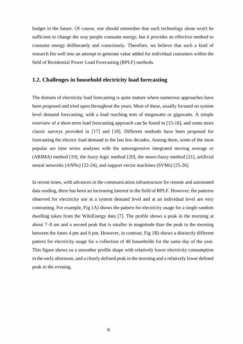
In recent times, with advances in the communication infrastructure for remote and automated

data reading, there has been an increasing interest in the field of RPLF. However, the patterns

observed for electricity use at a system demand level and at an individual level are very

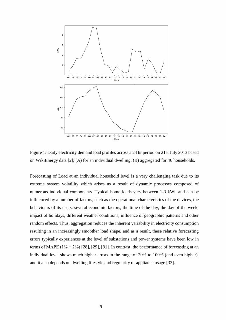
contrasting. For example, Fig 1A) shows the pattern for electricity usage for a single random

dwelling taken from the WikiEnergy data [7]. The profile shows a peak in the morning at

about 7–8 am and a second peak that is smaller in magnitude than the peak in the morning

between the times 4 pm and 6 pm. However, in contrast, Fig 1B) shows a distinctly different

pattern for electricity usage for a collection of 46 households for the same day of the year.

This figure shows us a smoother profile shape with relatively lower electricity consumption

in the early afternoon, and a clearly defined peak in the morning and a relatively lower defined

peak in the evening.

9

Figure 1: Daily electricity demand load profiles across a 24 hr period on 21st July 2013 based

on WikiEnergy data [2]; (A) for an individual dwelling; (B) aggregated for 46 households.

Forecasting of Load at an individual household level is a very challenging task due to its

extreme system volatility which arises as a result of dynamic processes composed of

numerous individual components. Typical home loads vary between 1-3 kWh and can be

influenced by a number of factors, such as the operational characteristics of the devices, the

behaviours of its users, several economic factors, the time of the day, the day of the week,

impact of holidays, different weather conditions, influence of geographic patterns and other

random effects. Thus, aggregation reduces the inherent variability in electricity consumption

resulting in an increasingly smoother load shape, and as a result, these relative forecasting

errors typically experiences at the level of substations and power systems have been low in

terms of MAPE (1% − 2%) [28], [29], [31]. In contrast, the performance of forecasting at an

individual level shows much higher errors in the range of 20% to 100% (and even higher),

and it also depends on dwelling lifestyle and regularity of appliance usage [32].

10

1.3. Problem statement

Due to the introduction of renewable energy resource and its unpredictable nature, the energy

demand forecast has become very complicated. Thus, their requirement of a robust

forecasting method which can make accurate energy demand prediction for a very short

frequency and accuracy. If we split the electricity market into different components, then

there is a significant proportion of demand comes from households.

Household energy demand depends on various factors like the area of a house, member count,

appliances used, outside temperature, weekdays, etc. The prediction of household energy

demand based on the number of devices poses a significant challenge due to variability in the

number of devices, types of devices and non-uniformity of the data. Hence, it is essential to

come up with a new way of forecasting household energy demand.

Here, in this thesis, we will try to study an approach to forecast the various hourly electricity

loads of individual consumers for a full 24 hours by considering historical electricity

consumption and also the household's behavioral data. In particular, based on historical data,

we aim to provide answers to the following research questions:

1. The possibility to provide accurate load forecasting for 24 hours on the individual

household level and to what extent if it is viable?

2. Are clustering and ARIMA algorithms right tools for identifying patterns of household

behavior? And are these forecasting methods and algorithms appropriate to address such high

volatility data?

1.4 Contribution of the thesis

Overall, we first cluster together houses with similar energy consumption pattern based on

the hourly energy consumption pattern over a week. And then for each cluster we build the

best model by statistical time series methods for energy consumption forecasting.

• We Identified similar houses based on their energy consumption profile and cluster

them together. Now for new house we will just need to identify the specific cluster it

belongs, and more accurate forecasting could be done.

• We created forecasting model to forecast more accurately for the next 24 hours energy

requirement for a given house.

11

• We provided an efficient data analysis strategy to that will facilitate optimization of

energy usage in residential buildings which will enable optimal control of internal

sub-systems and also allow for an efficient interaction with external systems like

electricity producers.

12

Chapter 2

2.1. Literature Review

The following section presents a brief review of existing literature about the methods which

are commonly applied for forecasting household energy consumption.

2.2. Review of application studies on ARIMA

ARIMA models are among the basic and most general form among the different forms of

time series forecasting techniques. They are based on the idea of transforming the fluctuating

time series to be stationary by the using differencing methods and processes

Newsham and Birt [33] have developed an ARIMAX (Auto-Regressive Integrated Moving

Average with eXternal (or exogenous) input) based model for forecasting the power demand

for an office building. They took use of occupancy data as an external predictor for improving

their model. Data for Hourly consumption was collected for 79 days from which 5 complete

days of network login data and 17 full days of motion sensor data was missing. These values

were imputed by using the mean of the non-missing values for the same hour and week. The

MAPE for both the cases of with occupancy and without occupancy data were found to be

1.217 and 1.244 respectively, implying that when occupancy is considered, there is a slight

improvement in accuracy of forecasting.

Yao et al. [34] used a combined forecasting model which was based on an Analytical

Hierarchy Process (AHP) to predict the hourly cooling load. Here, AHP was used to deduce

the weights of several models that were then integrated to improve the forecasting accuracy.

More details on AHP can be found in the work of Saaty [52,53]. For that study, three elements

were used to determine the ‘local priority'. These were known as the degree of fitting to the

historical data, adaptability, and reliability. The weights obtained for ARIMA, GM and ANN

model, were 0.564, 0.218 and 0.219 respectively.

Wang and Meng [35] have developed a hybrid model consisting of neural network and

ARIMA models to forecast the energy consumption for the entire province of Hebei in China.

They have used data for annual energy consumption from the year 1980 to 2008 to develop

13

and test the model. This ARIMA model was then used to take care of the linear aspects of the

data, whereas, the ANN was used to take care of the non-linear part. After this, results taken

from the ANN were used to predict the error term of the ARIMA model. The MAPE for this

hybrid model was very impressive at 0.311%.

Kandananond [36] has used ANN, ARIMA and multiple linear regression (MLR) for

forecasting the electricity demand for Thailand. The data used was from the year 1986 to the

year 2010. Subsequent results showed that the MAPE obtained was 0.996% for ANN and

those obtained for ARIMA and MLR were 2.809% and 3.260% respectively. However, the

results from the paired test showed that there was no significant difference between these

methods at α=0.05 and therefore, the ARIMA and MLR methods are preferable to the ANN

accounting for the simplicity of their structure.

Chujai et al. [37] have performed time series analysis for the household electricity

consumption using ARIMA and ARMA models. The data used to develop the model was

from the December of 2006 to November 2010. Subsequent results showed that the ARIMA

model could most suitably represent the forecasting periods for monthly and quarterly basis

and the ARMA model can most suitably represent forecasting periods in daily and weekly

basis respectively. The forecasting periods found most suitable for short-term periods were

ranging from 28 days, five weeks and towards six months to 2 quarters for long-term.

Roken and Badri [38] have used different multivariate techniques such as ARIMA and

dynamic regression econometrics techniques for forecasting the monthly peak load of

electricity for the city of Dubai. They have utilized the monthly data from January 1985 to

March 2007 and have taken 267 cases. The forecasting accuracy (coefficient of determination,

R2) between the actual data and the result obtained from the model was 0.997. This was for

the data between April 2006 and March 2007.

Zhuang et al. [39] have studied on building a load prediction model which is based on the

time series method and neural networks methods. Initially, the seasonal model which mostly

focussed on the analysis of the periodicity of the sequence is developed. After that the left-

out residuals obtained from the ARIMA model are modeled using ANN. Such a study was

done for over one week of data and the results which were obtained showed that the combined

model was superior to a simple time series model. However, no error analysis was provided.

14

Abdel-Aal and Al-Garni [40] have used ARIMA models to forecast the monthly electric

consumption. They have taken data for the past five years and have forecasted new data for

the sixth year. The model derived here is a multiplicative combination of the seasonal and

non-seasonal levels. The model structure was named ARIMA (1, 1, 0) (1, 1, 0)12. Such

ARIMA models were found to be more accurate and requiring lesser data when compared to

other regression and abductive network-based machine-learning models. Here, the average

percentage error for the ARIMA model was 3.8%.

Abosedra et al. [41] have estimated the demand for in Lebanon using a combination of

Ordinary Least Square (OLS), ARIMA and exponential smoothing methods. The monthly

electricity data for one full year was used to develop an ARIMA (0, 1, 3) (1, 0, 0)12 model.

It was subsequently found that this ARIMA model is much superior to the simple OLS and

exponential models and it resulted to a RMSE of 42.06 for monthly electricity consumption.

Almeshaiei and Soltan [42] have developed a methodology to forecast the daily electric power

load by utilizing the daily electricity data for the city of Kuwait. The methods used for

forecasting was divided into five parts – (1) A Primal visual and descriptive statistical

analysis; (2) contour construction; (3) Load pattern decomposition; (4) Load pattern

segmentation; (5) Future load forecasting. This above model was then developed using the

data from three years, and the MAPE was found to be 0.0384%. Tserkezos [43] then

developed Box-Jenkins ARIMA based models for forecasting the residential electricity

consumption for Greece using its monthly and quarterly data. The data were obtained for

fifteen years and a total of 180 observations respectively. The data was then divided into two

parts, 156 of these observations were used to train and develop the model and the rest 24

observations were then used to measure the performance of the model. The corresponding

MAPE that was obtained for the monthly model was 3.78% and that obtained for the quarterly

model was 7.69% respectively.

2.3. Review of application studies on Fuzzy time series

Azadeh et al. [44,45] introduced a fuzzy regression model which is a combination of both

classical regression and fuzzy techniques. The data for monthly electricity consumption from

April 1992 to February 2004 was used to construct the model in this case. The impacts of pre-

processing the data and subsequent post-processing on the performance fuzzy regression is

15

studied. The model proposed here shows superior results when compared with other machine

learning models like genetic algorithm (GA) and ANN and exhibits a MAPE of 0.0082%.

Bolturk et al. [46] combined use of fuzzy time series with Singh's method to forecast the

electricity consumption for a commercial building in Turkey. Singh's method [47] is a model

of third order that utilizes the historical data of year (n−2, n−1, and n) for the framing rules

to implement the fuzzy logical relation, Ai→Aj, where Aj is the current state and is the

fuzzified enrolments for year n+ 1. Two approaches were then considered where the first

approach entailed electricity consumption values for three different time periods within a day.

The other approach considered the total electricity consumption. The resulting RMSE which

was calculated for both these approaches were 467.567 and 490.310 respectively with a

difference of about 5% between them.

Efendi et al. [48] applied a linguistic out-sample based approach for the fuzzy time series and

applied it to the daily electricity load demand forecasting for Malaysia. This study formulated

a new rule for the determination of the weights of the fuzzy logical relationship (FLR) by

using index number of close relationship in the fuzzy logical group. The corresponding data

for the electrical load for eight months was considered at a daily basis for the analysis and the

resulting MAPE for a varying number of testing datasets was found to be below 1.63%.

Ismail and Mansor [49] have presented a fuzzy logic-based approach for the forecast of half-

hourly electricity load demand for Malaysia. Rules have been developed for factors each day

(working, weekend and holidays) and factors like temperatures and load using current load,

current temperature, previous load and previous temperature. A total of four defuzzification

methods are employed. The data used in the process is half-hourly electricity load for a week.

The results show a MAPE between 1.645% and 5.81% for the four defuzzification methods

chosen above.

Lim et al. [50] have proposed the chaos fuzzy controller model for the prediction of the short-

term electric power demand of a power plant. The input data in this case of the controller are

weather-related ones, like temperature, climate and the increase in temperature. The results

obtained show that the average error between the predicted data and actual recorded data was

5.65%. It was proposed that more weather-related data would improve the accuracy of the

model.

16

Liu et al. [51] have proposed a short-term electric load-based forecasting method using a

sliding window fuzzy time series to train the trend predictor in the training phase and use

these trend predictors to generate the forecasting values in the forecasting phase. The data

chosen was the hourly electric load for four days as the working examples. The maximum

MAPE from the model found to be 7.74% for the testing dataset.

Pei [52] has proposed an improved version of the fuzzy time series approach for load

forecasting. This approach utilized unequal-sized intervals partitioning based on a K-means

algorithm along with using an enhanced fuzzification method. Data for a day was analyzed

on hourly intervals to build the forecasting model. The results obtained show that the

prediction accuracy is highest by using a fuzzy time series of order 4, and a forecasting model

with 8 clustering partition on the domain.

2.4 Review of application studies on hybrid models

2.4.1 ARIMA+ANN

Wang et al. [53] have proposed an approach for the forecasting of a short-term load by

applying wavelet de-noising approach using a combined model of ARIMA and ANN. The

wavelet transformation first categorizes an approximate part which is associated with low

frequency and a then a detailed part which is associated with higher frequencies. The data for

an hourly electrical load of New South Wales (Australia) for 4 weeks was taken and then was

used to train and validate the model. The results obtained show that the proposed wavelet

denoising based combined model (WDCM) exhibits a MAPE of 0.016% which is lower than

the individual models like SARIMA, BPNN and the combined model which was without

wavelet de-noising.

Zhuang et al. [54] have presented a combined prediction method by combining ARIMA and

ANN models. The dataset, in this case, is obtained by building simulation software, DeST.

The load data taken from July 1 to July 31 is used to develop the model and the corresponding

data of the first week of August is used to test the model. The result obtained shows that the

17

combined model is superior to the standard time series model and solves the problem of

nonlinearity fitting as well.

2.4.2 ARIMA+ Evolutionary algorithms

Yang et al. [55] have proposed the evolutionary programming approach to help identify the

ARMAX model for forecasting of the short-term load. The hourly data for four seasons along

with the temperature data for three Taiwan cities are taken for analysis. The results obtained

show that for all the seasons, the model proposed had a maximum error of 2.27% and was

superior when compared to the traditional gradient search-based approach.

Huang et al. [56] have proposed a particle swarm optimization (PSO) based approach for the

identification of the ARMAX model for the forecasting of the short-term load. Data for four

seasons along with temperature data for three Taiwan cities are taken for analysis at an hourly

interval. The results obtained show that for all these reasons, the proposed PSO based model

has an error lower than 2.55%.

Wang et al. [57] has proposed an ARMAX model based on the evolutionary algorithm and

also a particle swarm optimization for forecasting of the short-term load. The data used for

this study is a real-time hourly load during summer for 2 months in the year 2005. The

weekends and weekdays are then analyzed separately. For the eight testing days, the proposed

model has obtained MAPE lower than 3.418%.

2.4.3 ARIMA+SVD+CONVEX HULL methods

Lu et al. [58] have proposed a new method which is based on a physical-statistical approach

for building a forecast for energy consumption. This physical model provides the theoretical

inputs which is underlying the energy flow mechanisms. Subsequently, stochastic parameters

are introduced, and a time series model is constructed using them which is then generalized

based on the convex hull technique. The data used for this analysis is taken from 4 sports

halls for 5 years between 2009 and 2013. The results obtained show that the RMSE for

electricity consumption for all different four sports halls was less than 10.15.

18

2.4.4 ARIMA+SVM

Nie et al. [59] have proposed a hybrid method based on ARIMA and SVM models to forecast

the short-term electricity load. The data is obtained from an electric power company in

Heilongjiang, China on an hourly basis for a period between March 1st and May 31st, 1999.

The MAPE which was obtained for this proposed hybrid method is 3.85% and when

compared, it was 4.5% and 4% from ARIMA and SVM models respectively.

2.5 Clustering

Most statistical methods utilize the historical data to construct probabilistic models to

estimate and analyze the future energy consumption. Generally speaking, these artificial

intelligence-based methods can obtain accurate prediction results in most real-world

applications and thus they have been widely applied to the prediction of building energy

consumption as well. In [60], cluster-wise regression models, a novel technique that integrates

both clustering and regression simultaneously was proposed for forecasting the consumption

of building energy. In [61], a clustering method was introduced to find the similarity of the

pattern for sequences of electricity prices and their demand prediction. In [62], a k-means

method was presented for the analyzing of the pattern of electricity consumption in case of

buildings.

Based on the literature review, it seems that there is a clear and increasingly recognizable

trend for research that looks at the challenges associated with different behavioral factors that

impact usage of energy for individual appliances at the household level. The rationale is also

to provide feedback on patterns of usage and to derive significant underlying associations

between the several contextual factors including usage time and user activities. It is expected

that these insights will increase the awareness and understanding of consumption of home

energy and may also be used as an additional variable that can enhance electricity forecasting

19

Chapter 3

3.1 Dataset

An openly available dataset named INTrEPID was used for this thesis

[https://cordis.europa.eu/project/rcn/105992_en.html]. The dataset consists of energy

consumption profiles for 58 different houses, each containing patterns of 3 to 9 individual

devices logged at a frequency of once every 2 minutes when idle and 2-8 seconds when in

use. The dataset was collected for the duration of 6 months to 1 year from households in

Denmark and Italy. Further, the dataset consists of power demand profile that was annotated

with various context values such as family size ranging from 1-5 adults per house, house area

ranging from 80-700m2, etc.

3.2 Problem Formulation

Due to the introduction of renewable energy resource and its unpredictable nature, the energy

demand forecast has become very complicated. Thus, their requirement of a robust

forecasting method which can make accurate energy demand prediction for a very short

frequency and accuracy. If we split the electricity market into different components, then

there is a significant proportion of demand comes from households.

Household energy demand depends on various factors like, the area of a house, member count,

appliances used, outside temperature, weekdays, etc. The prediction of household energy

demand based on the number of devices poses a significant challenge due to variability in the

number of devices, types of devices and non-uniformity of the data. Hence, it is essential to

come up with a new way of forecasting household energy demand.

Here, in this thesis, we will try to study an approach to forecast the various hourly electricity

loads of individual consumers for a full 24 hours by considering historical electricity

consumption and also the household's behavioural data. In particular, based on historical

data, we aim to provide answers to the following research questions:

20

1. The possibility to provide accurate load forecasting for 24 hours on the individual

household level and to what extent if it is viable?

2. Are clustering and ARIMA algorithms right tools for identifying patterns of household

behaviour? And are these forecasting methods and algorithms appropriate to address such

high volatility data?

21

Chapter 4

Background

4.1 Time Series Data

A time series is a sequence of data points, typically consists of sequential measurements or

observations on some quantifiable variable(s), which are made over a fixed time interval [1]

as depicted in figure 3.1 below. Usually, the observations are in chronological order and

taken at regular intervals (days, months, years), but the sampling can sometimes also be

irregular.

Some typical examples of time series are historical data on sales of products, inventories,

customer counts, interest rates, costs, etc. Time series data are also naturally seen in many

areas of application including:

• Economics - e.g., monthly data for unemployment, hospital admissions, etc.

• Finance - e.g., daily exchange rate, share prices, etc.

• Environmental - e.g., regular rainfall, air quality readings.

• Medicine - e.g., ECG brain wave activity every 2−8 secs.

According to [71], a time series can be represented by a collection of observations XT, where

each one is recorded at a specific time T; these are written as:

{X1, X2,...Xt } or {XT}, where T takes the values 1, 2,...t

If a time series has a regular pattern or a trend, then the value at any point of the series should

be a function of corresponding previous values. If the target value that is to be modeled and

predicted is X, and Xt is the value of X at any time t, then the goal of this approach is to

create a model of the form:

Xt = f(Xt-1, Xt-2, Xt-3, …, Xt-n) + et

Where Xt-1 is the value of X for one previous observation, Xt-2 is the value two

observations in the past and so on, here, et represents the noise that does not follow any

predictable pattern (this is called a random shock). The values for the variables which occur

before the current observation are called lag values.

22

If a time series shows a repetition in its pattern, the value of Xt is usually very highly

correlated with its Xt-cycle where the cycle is the number of observations in the pattern

(DTREG, 2010). For example, monthly observations with an annual cycle often can be

modeled by:

Xt = f(Xt-12)

Generally, time series models do not differ much from the rest of econometric models. The

significant difference here is that the variables are subscripted with T rather than the normal-

conventionally-used i. According to [72], a straightforward method for the description of a

series is the method of classical decomposition. Classical decomposition has the notion that

a time series can be decomposed into four elements:

Trend (Tt) — The trend is any long-term movements in the mean of the series. A long-term

trend is typically modeled using a linear, quadratic or exponential function.

Seasonal effects (It) — Seasonal effects are cyclical fluctuations that relate to the calendar;

Cycles (Ct) — Cycles are other cyclical fluctuations (such as a business cycle etc.). In this

case, an upturn or downturn is not tied to seasonal variation. These usually result from

changes in economic conditions.

Residuals (Et) — Residuals are other random or systematic fluctuations which cant be

explained.

The idea is to create separate models for all these four elements and then combine these

elements. This can be done in two ways, either additively

Xt = Tt + It + Ct + Et

or multiplicatively

Xt = Tt * It * Ct * Et

The objective of time series data is to determine the pattern of the time series. Here the

model describes the essential features of the time series, explains the interaction between

time lags along with forecasting the future time series value.

23

Figure 4.1: Time Series data plot [78]

The figure shows a typical time series data of a number of births per year from 1946 to 1960.

4.2 Basic Concepts of Time Series

There is a vast amount of existing academic literature within the domain of time series

analysis and its concepts. A time series can be categorized into two major classes namely:

univariate or multivariate. A univariate time series is a sequence of measurements for the

same variable collected over time. Mostly, these measurements are a sequence of events that

occur at regular time intervals. An event is defined as an ordered pair which consists of a

temporal value and a corresponding list of metadata (attributes) which are also known as the

header or the general description [73]. A typical univariate time series has the following

format:

{(t1, data-value1), (t2, data-value2), ... , (tn, data-values)}, for i= 1,2,…,n

Where data-value is the data value for the corresponding time ti.

However, when a time series has more than a single variable, it is called to be multivariate.

Most of the economic and financial indicators are structured in this for. These can be further

classified into homogeneous and heterogeneous multivariate time series, by the relationships

between the different measured variables. If a variable X is found to be useful to predict the

future values of another variable Y, then the multivariate time series is called homogeneous;

otherwise, it is heterogeneous. In the case of homogenous multivariate time series, a change

24

in any one element in the observations vector of one variable also implies corresponding

changes in other variables belonging to the process under study.

Multivariate time series have the following general format:

{(t1, < data-value11, data-value12, ... >), (t2, < data-value21, data-value22, ... >), (tn, < data-

valuen1, data-valuen2, … >)}.

4.3 Components of Time Series Data

A time series has 4 components [74]:

1. Trend

2. Seasonal

3. Cyclic

4. Irregularity

1. Trend (T): It is a long-term smooth variation (increase or decrease) in the time series.

Figure 4.2: Time Series plot showing increasing trend in the data [75].

2. Seasonality (S): Seasonality is present when there are seasonal patterns in the data.

Seasonality can be daily, weekly or monthly. For example, similar consumption patterns

over the years for the summer season, more consumption on weekends, every day more

use in the morning than evening [75].

Figure 4.3: Seasonal Plot is showing a seasonal pattern in the data over the years[75].

3. Cycle(C): Cyclic patterns are rise and fall of an unfixed period. These are not seasonal

patterns. Figure 4.4 shows a cyclic pattern over the years1

25

Figure 4.4: Cyclic Plot is showing a cyclic pattern in the data over the years [75].

Irregular component(I): The random, unpredictable variation in the time series is called an

irregular component. Figure 4.5 shows irregular birthrate over the years.

Figure 4.5: Irregular component plot. Abrupt changes in the data [75].

4.4 Time Series Analysis

The occurrences of time series data are becoming extremely valuable to the field of

operations and development for organizations. Financial institutions, for example, rely on

time series analysis for the forecasting indicators like economic conditions, the development

and use of some complex financial decision support models, and conducting financial

transactions internationally. Similarly, many public and private institutions are also using

time series data to manage and predict the loads on their respective networks [74]. Therefore,

an understanding of the basic practices a time series analysis is adequate for the reader. The

next paragraph explains the various processes, , and objectives of a time series analysis. It

also discusses the uses and relevance of such time series models as well as categorizes them.

26

Time series analysis helps when all the data points have been taken over time and have an

inner structure (such as autocorrelation, trend or seasonality) which needs to be accounted

for. As has been written earlier, time series analysis is composed of methods and steps which

analyses time series data and extracts meaningful statistics and some other useful

characteristics from the data. The process also involves the use of various techniques for

drawing inferences from the time series data. Forecasting is the application of such a model

to predict future values based on previously observed time series values [74].

For performing a time series analysis, it is essential to set up a hypothetical probabilistic

representation of the data we have. Such a description is called the Model. Once the model

is determined appropriately, it is then possible to estimate the various parameters, check for

the goodness of fit to the data, and then to possibly use the formulated and fitted model to

enhance the understanding of the mechanism behind the series [74]. Once an appropriate

and satisfactory model has been developed, it is used in anyways depending on the particular

nature of the application.

4.5 Forecasting Methods

Two forecasting methods which have complementary approaches are the ARIMA model

and the Exponential Smoothing method. The ARIMA model is used to describe the auto-

correlation within the data while the Exponential Smoothing method takes the trend and

seasonality of the data as its basis. In addition to these, there are some advanced approaches

for the forecasting of data as well.

A brief description of these methods is given below:

ARIMA models: ARIMA stands for autoregressive integrated moving average which is a

generalization of the auto-regressive and moving average (ARMA) model. The MA (moving

average) part models the past error terms and the AR (autoregressive) part is used to regress

on its own lagged values [74].

Exponential Smoothing: This method is used the weighted averages of past observations,

exponentially decaying weights as the observations get older, i.e., a higher eight is associated

with a more recent observation. Exponential smoothing methods can of various types such

as simple exponential smoothing, the Holt's linear trend method, the Exponential Trend

method, the Holt-Winters seasonal method, among others. The variations between these

27

methods account for the presence of trend and seasonality within the data, i.e., the method

is modified according to the presence of these characteristics in the time series data [74].

Advanced Forecasting Methods: For many problems, there is a need to modify existing

models to suit the model well. For the example of the energy domain, we use a Multi-

Seasonal Exponential smoothing method which is a modified version of the Holt-Winter

Exponential Smoothing model. Another such modified model is EGRV which is a multi-

equation model using sub-models concerning daily data granularities [74].

4.6 Clustering

The process of bringing together objects having similar features i.e. grouping similar objects

together is known as Clustering. This is used to simplify the data analysis. Objects from one

cluster may be varyingly different from another cluster, and thus they may require different

techniques for their modeling. Some popular clustering techniques are k-means clustering,

Fuzzy C means clustering and hierarchical clustering etc. Figure 3.6 illustrates the difference

between clustered and raw data.

28

Figure 4.6: Clustering of data [76].

The figure 4.6(A) depicts raw data before clustering. The figure 4.6(B) depicts raw data after

k-means clustering. Three clusters can be seen in data in different colors. The green and blue

clusters are scattered while the red one is compact with few outliers.

29

Chapter 5

5.1 Data analysis methodology

Before selecting an appropriate model, the data needs to be prepared in a uniform and useable

time series format. Analysing the time series gives us a general idea of what approaches may

work, what are the chances of outliers being there, how well the data needs to be pre-processed

before applying the model. The general scheme of the analytical procedure is represented in

Figure 5.1

Figure 5.1: Schematic representation of complete data analysis procedure

The data analysis methodology comprises 3 significant steps. The data is pre-processed and a

time series data frame is created with hourly energy consumption for each house.

Data Processing

• Creating data frame with hourly energy consumption for each unit

• Creating data frame with hourly consumption for each house

Clustering

• Clustering the houses based on the energy consumption using DTW Fuzzy c means clustering

• Creating time series for each cluster

Forecasting

• Creating HoltWinters, ARIMA, ETS and Snaive model for each cluster

• Comparing the models w.r.t. error(MAE, MAPE, MaxAE & Sigma) to find the best model.

30

Project Outline

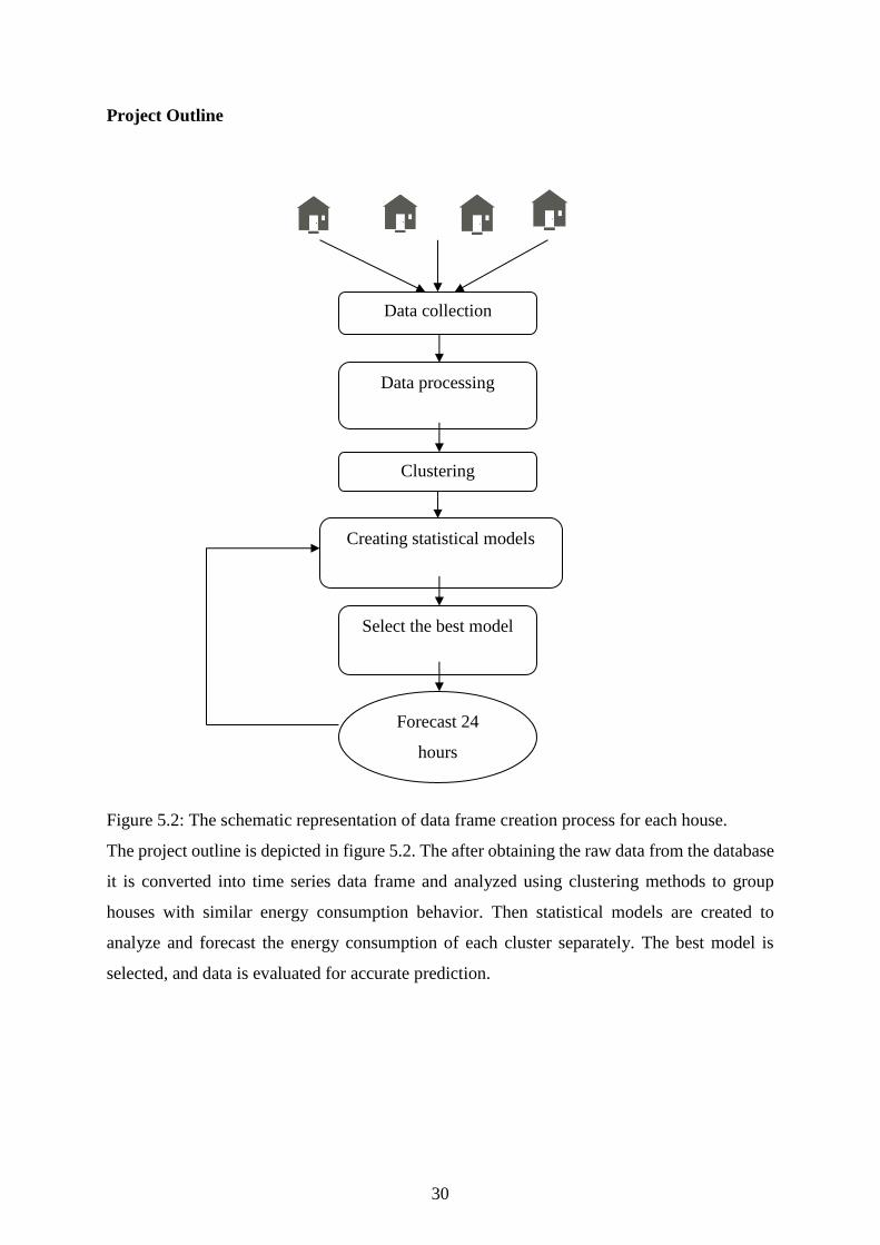
Figure 5.2: The schematic representation of data frame creation process for each house.

The project outline is depicted in figure 5.2. The after obtaining the raw data from the database

it is converted into time series data frame and analyzed using clustering methods to group

houses with similar energy consumption behavior. Then statistical models are created to

analyze and forecast the energy consumption of each cluster separately. The best model is

selected, and data is evaluated for accurate prediction.

Data processing

Clustering

Creating statistical models

Select the best model

Forecast 24

hours

Data collection

31

5.2 Trend and Seasonality

Here we begin with the time series analysis of the time series data we have generated. We look

for any trend in the data. If there is any trend, we de-trend the time series and look for the

seasonality. Now the seasonality could be daily, weekly and monthly. Like on a daily basis we

may have more consumption in the morning and evening than compared to rest of the day. On

a weekly basis, we may have more consumption on weekends than on weekdays. Similarly, we

have different patterns of power consumption for winter and summer.

5.3 Aggregation-level-dependent-Predictability

Next, we may look for energy consumption profiles for various households, and if they are

found to be similar, can aggregate them together. This will lead to lower forecast error as it

will compensate for fluctuations of a single household which may be significant and abrupt.

Aggregation can also be done at the device level but is beyond the scope of this project. Also,

we can change the temporal resolution from 15 min to 30 min or 1 hour depending on what

gives better predictable time series. We can even average the energy consumption of past four

Sundays where no special event occurred to improve forecasting.

5.4 Clustering

Before moving on to forecasting, clustering can be used as a pre-processing step where we

cluster households by the similarity of consumption of energy, i.e., their energy profile. This

in a way also helps in classifying user behavior. As each cluster would have specific feature

values associated with it which distinguishes it from another. This helps to know the sub-

structure of the data. One can train a particular classifier on a cluster of households or devices.

We can also get the novel features performing cluster analysis which can be further used to

predict unknown object. We can also show outlier analysis that hinders the learning process.

Before clustering we may use dimensionality reduction technique like principal component

analysis to reduce the dimension of the dataset, i.e., we select some features for clustering.

Before clustering, we pre-process data depending on the type of clustering like normalization

32

and the use clustering algorithm: ‘Fuzzy C Means clustering”. Once the clusters have been

formed, we can assign a new device or a household to a cluster using standard decision tree

classifier. Along with clustering, we can perform outlier mining to analyze households with

unexpected energy consumption (figure 5.3).

.

Figure 5.3: Schematic representation of the procedure for clustering

The household with similar energy consumption patterns is clustered together using Fuzzy c-

means clustering. The ‘C’ clusters are obtained after the analysis.

5.5 Forecasting

Two types of models can be used for forecasting:

1. Multi-purpose general forecasting approaches.

2. Energy domain forecast models.

Calculate DTW

ACF Matrix

Apply Fuzzy c-

means clustering

N house time

C Clusters

Clustering

complete

33

The data is first randomly divided into training and test datasets. The analysis is performed on

the training set and forecasting performance evaluated using test data set. The first category

includes the exponential smoothing using Holt winters technique to capture the seasonality in

the data, auto-regressive model, and machine learning using S-Naïve forecasting technique.

We analyze the data and accordingly find the best fit model (Figure 5.4). The second category

comprises multi-seasonal exponential smoothing and a multi-equation model that uses

individual sub-models w.r.t. to daily data granularity. An example is multi-equation forecast

model using auto-regression.

Figure 5.4: Schematic representation of the procedure for time series analysis.

Create train and test dataset Rep

eat the p

rocess fo

r all the clu

sters

Create time series for the

cluster

Cluster

Build models

Holt- ARIMA ETS S-Naive

Select the best model

Forecasting for

next 24 Hours

34

Each cluster is converted into a time series data frame. The data frame is further analyzed to

predict future energy consumption using the forecasting methods like Holt, ARIMA, ETS, and

S-Naïve. The resulting best model is applied on the test data.

5.6 Time Series Context and Context drifts

The energy consumption dataset is driven by a conglomeration of background processes and

external influences. These influences can be categorized into three broad categories:

1. Calendar: Special days, public holidays, vacation seasons.

2. Meteorological: Temperature, cloudiness, rainfall.

3. Economic: Local laws.

The state of influence factors are not stated but rather change over time and without entire

series context. The changes are called context drifts. These can be abrupt like example

sports, gradual like slow transformation on increasing ecological awareness or cyclic drifts

on seasonal patterns.

Now we can find correlation via observation and incorporate into our forecasting model.

For auto-regressive models, we can use AR(I)Max which allows inclusion of exogenous

variables by additively or multiplicatively adding a term for the exogenous variable to the

equation.

35

Chapter 6

6.1 Analysis

This chapter presents the results of analyzed data set as per the methodology mentioned in

Chapter 4.

Early Analysis:

1. Data was captured in watts.

2. While the device was idle, the data was captured at an interval of 2 minutes and the

readings varied between 1-2 watts.

3. When the device was in use, the readings were captured at an interval of 4-8 seconds,

and the reading varied between as per the consumption of the device.

There are a total of 58 houses in the data set which contain 442 electrical devices in each house

has 3 to 9 appliances with an average of 7 appliances each.

Figure 6.1: No. of devices per house

The number of houses with 9 devices is highest (20). The minimum number of devices in a

house is 2.

36

Figure 6.2: Most common devices

It was found that there are 30 homes which have more than one unit of one type of appliance.

An oven is found in the most number of houses and television in the least.

6.2 Data Manipulation/Engineering

Since the time interval is not constant, to make the time series regular the time series was

converted to an hourly period using the the.hourl () function in R.

The maximum value of energy used for the hour is used to create the predictive model as this

would be the maximum watt needed to be supplied to the house. We also added the energy

consumption for all the devices of the house to access the overall energy consumption of the

given house. The time series started at "2014-11-14" and ended at “2015-11-14" hours.

However, the duration varied for some houses and also there are many periods when the data

is missing (not captured) for the device/house.

To make the time series regular a data frame is created with one column with an index with

hourly time (from start to the end of the time series) and another column watt to capture the

energy consumption readings. And the watt readings were filled matching the time series time

in the data frame (only hour and date was considered from the time series to match data).

37

For the missing value's data is filled in with the assumption that the pattern of using household

devices are likely to be repeated every week, a naïve method is used with the data of previous

week to fill the missing values using the for loop.

This process is repeated for each device in the dataset, and another data frame is created with

information of all the devices captured as a column with an index as hourly time series, as

represented in Table 1.

Table 1: Data Frame with unit-wise readings of energy consumption.

Now, the readings for the given hour was added, and another data frame was created with the

reading for all the devices of the given house. This data frame has energy consumed for the

given house in each column in that particular hour.

Table 2: Data Frame with house-wise readings of energy consumption.

The outliers in the data were replaced by the median value of the device reading when in use.

Since the exact reason for such variable reading is unknown; these outliers are replaced by the

median watt consumption for the device while it is in use.

38

6.3 Clustering of household energy consumption

Since the data is now being regularised and data for all the houses are converted into a time

series format. The houses will be clustered based on their energy consumption profile.

For a time series, Dynamic Time Warping distance can be used as a dissimilarity measure. This

is a shape-based clustering method. The calculation of the DTW uses dynamic programming

that tries to find the optimum path wrapping. However, this is computationally expensive in

both aspects time as well as memory.

Since the length of each time series is 8760 and entire 58-time series are available, hierarchical

clustering and K-means clustering is computationally very expensive, So Fuzzy C means

clustering method is used. We will perform autocorrelation based fuzzy clustering which will

also take care of the varied lengths of the time series. Starting with 20 clusters and check by

the shapes of different clusters, optimum numbers of clusters will be decided.

Code Snippet 1: for Fuzzy c- Means clustering with 20 clusters

# Calculate autocorrelation up to 100th lag

acf_fun <- function(dat, ...) {

lapply(house_df[5:62], function(x) {

as.numeric(acf(x, lag.max = 100, plot = FALSE)$acf)

})

}

# Fuzzy c-means

fc <- tsclust(house_df[5:62], type = "f", k = 20L, preproc = acf_fun, dis

tance = "L2",seed = 42)

plot(fc)

From the graphical analysis of all the clusters, they can be grouped based on their similarity as

follow:

a. 1, 8, 16

b. 2, 3, 11, 18

c. 5, 6, 15

d. 7, 9, 10, 12, 17, 20, 4

e. 13, 14

f. 19

39

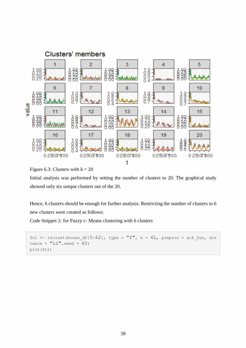
Figure 6.3: Clusters with k = 20

Initial analysis was performed by setting the number of clusters to 20. The graphical study

showed only six unique clusters out of the 20.

Hence, 6 clusters should be enough for further analysis. Restricting the number of clusters to 6

new clusters were created as follows:

Code Snippet 2: for Fuzzy c- Means clustering with 6 clusters

fc1 <- tsclust(house_df[5:62], type = "f", k = 6L, preproc = acf_fun, dis

tance = "L2",seed = 42)

plot(fc1)

40

Figure 6.4: Clusters with k = 6

The analysis was re-performed using a fixed number of clusters as 6.

Checking the number of houses in each cluster and the mean of each cluster

Cluster 1 Cluster 2 Cluster 3 Cluster 4 Cluster 5 Cluster 6

6 18 16 8 8 2

Table 3: Number of houses belonging to each of the clusters.

Six houses were classified in cluster 1, 18 in cluster 2, 16 in cluster 3, 8 in cluster 4 and 5 and

2 in cluster 6.

Figure 6.5: Clusters density

The pie chart depicts the density of houses classified in each cluster. Cluster 2 had the highest

density while cluster 6 had least.

Cluster 110%

Cluster 231%

Cluster 328%

Cluster 414%

Cluster 514%

Cluster 63%

Cluster Density

41

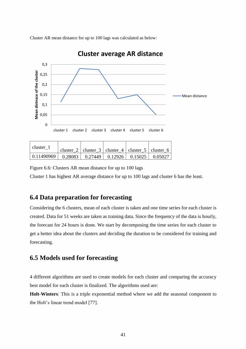
Cluster AR mean distance for up to 100 lags was calculated as below:

Figure 6.6: Clusters AR mean distance for up to 100 lags

Cluster 1 has highest AR average distance for up to 100 lags and cluster 6 has the least.

6.4 Data preparation for forecasting

Considering the 6 clusters, mean of each cluster is taken and one time series for each cluster is

created. Data for 51 weeks are taken as training data. Since the frequency of the data is hourly,

the forecast for 24 hours is done. We start by decomposing the time series for each cluster to

get a better idea about the clusters and deciding the duration to be considered for training and

forecasting.

6.5 Models used for forecasting

4 different algorithms are used to create models for each cluster and comparing the accuracy

best model for each cluster is finalized. The algorithms used are:

Holt-Winters: This is a triple exponential method where we add the seasonal component to

the Holt’s linear trend model [77].

cluster_1 cluster_2 cluster_3

cluster_4

cluster_5 cluster_6

0.11490969 0.28083 0.27449 0.12926 0.15025 0.05027

0

0,05

0,1

0,15

0,2

0,25

0,3

cluster 1 cluster 2 cluster 3 cluster 4 cluster 5 cluster 6

Me

an d

istn

ace

of

the

clu

ste

r

Cluster average AR distance

Mean distance

42

In this method alpha, beta and gamma coefficients are used for base value(u), trend

component(v) and seasonal component(s) smoothening. The three components for the next

period(i+1) are smoothened by using the previous period(i) and same period(i-c) for last

seasonal cycle.

If c is the cycle length, c= 7 for days in a week, c=12 for a month in a year and c=24 for hours

in a day.

Below are the equations to calculate the y(i+1), forecast for the next period.

The smoothening coefficients used in the model creation for all the clusters are as below:

Cluster alpha beta gamma

1 0.1628574 0 0.2105621

2 0.04228719 0.0003514562 0.3208938

3 0.02425709 0.001278881 0.3583316

4 0.5077053 0 0.4132362

5 0.04214828 0 0.2140286

6 0.7385532 0 0.1516631

Table 4: Smoothening coefficients used for HW models.

ARIMA: ARIMA stands for autoregressive integrated moving average which is a

generalization of auto-regressive and moving average model. We will be using the auto.arima()

function of the R “forecast” package. This function calculated the best AR, difference and MA

factors wrt the dataset used for training [77].

p/P= order of the autoregressive part;

d/D= degree of first differencing involved;

q/Q= order of the moving average part.

https://i0.wp.com/www.real-statistics.com/wp-content/uploads/2018/03/image159d.png

https://i1.wp.com/www.real-statistics.com/wp-content/uploads/2016/03/image004z.png

https://i2.wp.com/www.real-statistics.com/wp-content/uploads/2018/03/image160d.png

https://i0.wp.com/www.real-statistics.com/wp-content/uploads/2016/03/image012z.png

43

Hence, the formula for forecasting:

y′t=c+ϕ1y′t−1+⋯+ϕpy′t−p+θ1et−1+⋯+θqet−q+et

The best p, d and q values found for each of the clusters are below:

Cluster p d q P D Q

Cluster 1 1 1 2 0 0 2

Cluster 2 5 1 0 2 0 0

Cluster 3 5 1 0 2 0 0

Cluster 4 1 1 2 0 0 2

Cluster 5 0 1 2 0 0 2

Cluster 6 5 1 0 2 0 0

Table 5: (p,d,q) and (P,D,Q) values used for ARIMA models.

ETS: ETS stands for Error Trend and seasonality. This is also an exponential smoothening

forecasting method. This is a non-stationary algorithm. This model also provides if the

components are additive, multiplicative or not available (A-additive, M-Multiplicative and N-

Null) and uses alpha, beta and gamma as smoothening coefficients for error, trend and

seasonality [77].

The parameters used in the models are:

Cluster ETS Alpha Beta Gamma

Cluster 1 (A, N, A) 0.2706 0 0.0529

Cluster 2 (A, N, A) 0.2457 0 0.0755

Cluster 3 (M, A, M) 0.2675 0.0001001133 0.0665

Cluster 4 (A, N, A) 0.3454 0 0.0572

Cluster 5 (M, N, M) 0.0528 0 0.0507

Cluster 6 (A, N, A) 0.2842 0 0.1197

Table 5: ETS model parameters.

S Naive: This is a seasonal naïve method, one of the most basic method. In this method, the

value of the same period of the previous season is forecasted [77].

.

6.6 Evaluation

The result of the different models created is compared in respect to the error parameters

generated by comparing with the actual readings (mean for the given cluster). Which of the

model is resulting into least error will consider as the final model?

44

Since the readings used are at a frequency of 1 hour, fore of 24 hours will be compared to the

actual energy consumption for the duration.

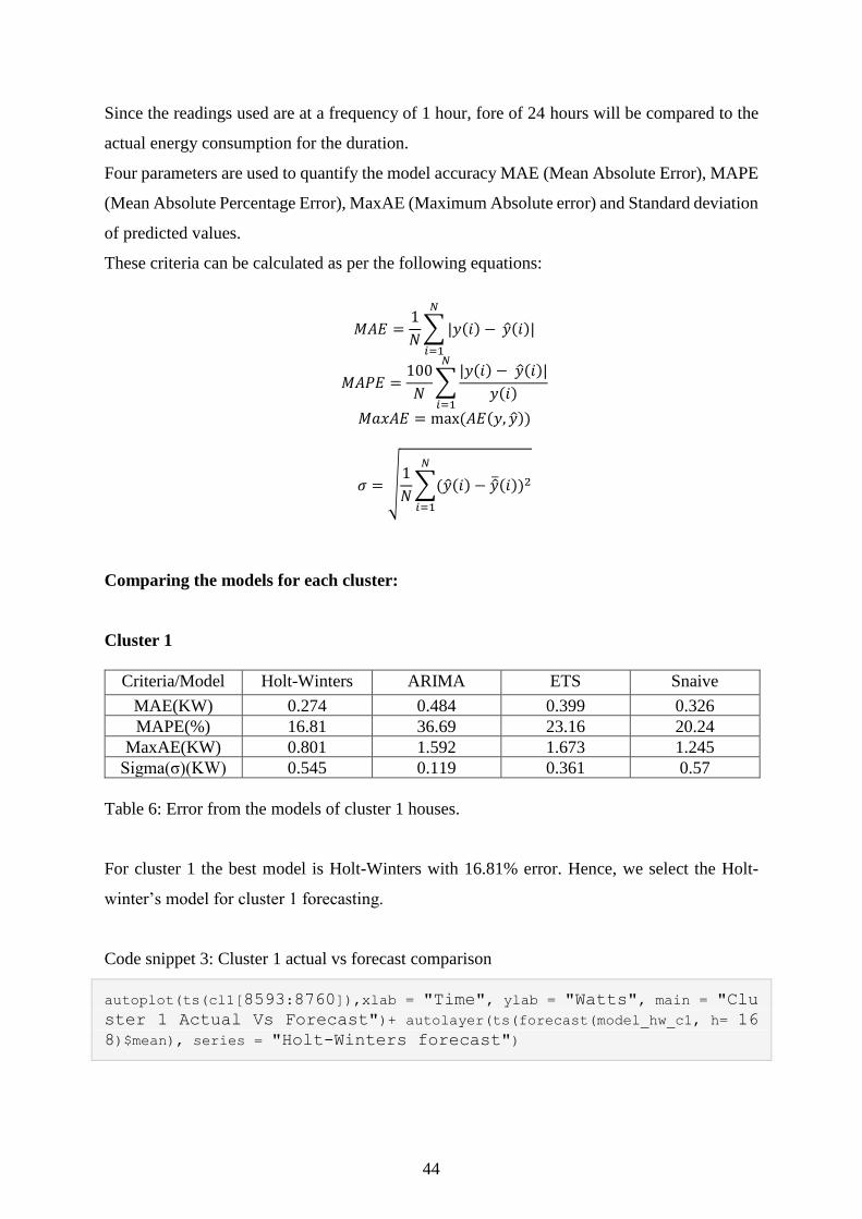
Four parameters are used to quantify the model accuracy MAE (Mean Absolute Error), MAPE

(Mean Absolute Percentage Error), MaxAE (Maximum Absolute error) and Standard deviation

of predicted values.

These criteria can be calculated as per the following equations:

𝑀𝐴𝐸 =1

𝑁∑ |𝑦(𝑖) −

𝑁

𝑖=1

�̂�(𝑖)|

𝑀𝐴𝑃𝐸 =100

𝑁∑

|𝑦(𝑖) − �̂�(𝑖)|

𝑦(𝑖)

𝑁

𝑖=1

𝑀𝑎𝑥𝐴𝐸 = max (𝐴𝐸(𝑦, �̂�))

𝜎 = √1

𝑁∑(�̂�(𝑖) − �̅̂�(𝑖))2

𝑁

𝑖=1

Comparing the models for each cluster:

Cluster 1

Criteria/Model Holt-Winters ARIMA ETS Snaive

MAE(KW) 0.274 0.484 0.399 0.326

MAPE(%) 16.81 36.69 23.16 20.24

MaxAE(KW) 0.801 1.592 1.673 1.245

Sigma(σ)(KW) 0.545 0.119 0.361 0.57

Table 6: Error from the models of cluster 1 houses.

For cluster 1 the best model is Holt-Winters with 16.81% error. Hence, we select the Holt-

winter’s model for cluster 1 forecasting.

Code snippet 3: Cluster 1 actual vs forecast comparison

autoplot(ts(cl1[8593:8760]),xlab = "Time", ylab = "Watts", main = "Clu

ster 1 Actual Vs Forecast")+ autolayer(ts(forecast(model_hw_c1, h= 16

8)$mean), series = "Holt-Winters forecast")

45

Figure 6.7: Clusters 1 actual vs Holt-Winter’s forecast for last week of the year

Cluster 2


MAE(KW) 0.267 0.330 0.335 0.336

MAPE(%) 20.51 35.94 30.42 25.23

MaxAE(KW) 0.72 0.736 0.784 0.854

Sigma(σ)(KW) 0.577 0.288 0.474 0.568

Table 6: Error from the models of cluster 2 houses.

The best model is Holt-Winters with minimum of 20.51% error. Hence we select the Holt-

winter’s model for cluster 2 forecasting.




8)$mean), series = "Holt-Winters forecast")

46

Figure 6.8: Clusters 2 actual vs. Holt-Winter's forecast for last week of the year

Cluster 3


MAE(KW) 0.23 0.281 0.274 0.395

MAPE(%) 32.35 29.93 43.06 41.96

MaxAE(KW) 0.603 1.191 1.027 1.038

Sigma(σ)(KW) 0.549 0.304 0.416 0.656

Table 7: Error from the models of cluster 3 houses

Though all the models have more than 30% error except ARIMA, Holt-Winters model gives

an error of 32.35% and least MAE /MaxAE. Also, when looking for the long-term(1week)

forecasting ARIMA leaves more substantial error that HW, Hence HW model is selected as

the best model for Cluster 3 houses for larger forecasting and ARIMA for shorter forecasting.




8)$mean), series = "HW forecast")

47


Cluster 4


MAE(KW) 0.373 0.390 0.327 0.415

MAPE(%) 7.75 7.76 6.65 8.45

MaxAE(KW) 1.12 1.417 1.264 1.956

Sigma(σ)(KW) 0.354 0.084 0.302 0.336


With least error of 6.65% we are considering ETS model as the best model for cluster 4.



ster 4 Actual Vs Forecast")+ autolayer(ts(forecast(model_ets_c4, h= 16

8)$mean), series = "ETS forecast")

48

Figure 7.1: Clusters 4 actual vs ETS forecast for last week of the year Cluster 5


MAE(KW) 0.235 0.305 0.251 0.323

MAPE(%) 19.45 27.66 21.98 27.99

MaxAE(KW) 0.621 0.609 0.755 0.981

Sigma(σ)(KW) 0.332 0.129 0.345 0.491


HW model has least error of 19.45 % is selected as the final model for cluster 5 houses.





49


Cluster 6


MAE(KW) 0.742 0.789 0.751 1.005

MAPE(%) 50.43 48.84 50.84 46.39

MaxAE(KW) 1.937 2.697 1.948 3.136

Sigma(σ)(KW) 0.66 0.390 0.658 0.743


Though all the algorithms are giving error of around 50 %, however the MaxAE for the ARIMA

and Snaive are too high, HW and ETS models are comparable with less MaxAE. We will go

with Holt-Winters.





50


51

Chapter 7

7.1 Discussion

First, we start the analysis with the selection of data set. In this case, we use the household

energy consumption data from open source INTrEPID database. This data was chosen because

it had information of energy consumption at the device and household level. We performed the

analysis at household level instead of the device level because it poses a significant challenge

due to variability in the number of devices, types of devices and non-uniformity of the data.

In this project, we have studied the behavior of different types of houses based on their energy

consumption profiles. This thesis presented several techniques for the prediction and analysis

of household energy consumption. We first clustered together houses with similar energy

consumption pattern based on the hourly energy consumption pattern over a week and found

six unique type of clusters out of the initial 20 clusters. For each cluster we build the best model

by statistical time series methods for energy consumption forecasting using Holt winter’s

technique, ARIMA, ETS and s-Naïve techniques. The best models for cluster 1, 2, 3, 5, 6 was

Holt winter’s forecasting method (Figure 7.4). Only cluster 4 was best analyzed using the ETS

model. We were able to achieve up to 93.35% accuracy for some of the clusters using

exponential smoothening methods like Holt-Winters and ETS models.

Figure 7.4: Graph comparing Mean Absolute Percentage Error for different models for all the

clusters.

0

10

20

30

40

50

60

Cluster1 Cluster2 Cluster3 Cluster4 Cluster5 Cluster6

Pe

rce

nta

ge E

rro

r

Model Comparision

Holt-Winters

ARIMA

ETS

Snaive

52

Comparing the error in forecasting Holt-Winter’s model result in the least error in 4 of the

clusters and very competitive errors in rest of the clusters. Also, considering the seasonal

behavior of energy consumption and error in the result Holt-Winter's model is found to be the

best performing model. Based on this model the energy demand planning could be improved

significantly.

7.2 Conclusion

To conclude we successfully showed an efficient method to analyze household energy

consumption data by performing several analysis. We showed that we could accurately predict

future energy demand by using specific techniques as per the data. However, the analysis is

still not automated and needs to be performed manually to identify the best model.

These results could be used for efficient management of energy devices and to predict future

energy demand of the household. It provides a solution for the stakeholders like energy

producers, consumers, government for efficient and smart usage of electricity and predicts

future outcomes.

7.3 Future Work

We also have identified several possible directions for future to improve the forecasting

accuracy as well as other studies which could help in planning for energy demand and supply

with the complexity of renewable and non-renewable energy management.

• Including factors like house area, no. of members of the house in clustering to

understand the relation between the energy consumption.

• Building more accurate models by including other external variables like outside

temperature, holidays using neural network models.

• To build models to understand the usage of household items and use them to make

efficient use of renewable energy, e.g., changing the time of electric car charging based

on the best availability of wind energy, etc.

• Building models at the device level to identify less efficient devices.

53

7.4 References [1] Hua, C.; Lee, W.L.; Wang, X. Energy assessment of office buildings in China using China

building energy codes and LEED 2.2. Energy Build. 2015, 86, 514–524.

[2] Zuo, J.; Zhao, Z.Y. Green building research-current status and future agenda: A review.

Renew. Sustain. Energy Rev. 2014, 30, 271–281.

[3] Hong T. Pinson P. Fan S. Global energy forecasting competition 2012. International Journal

of Forecasting. 2014; 30(2): 357–363.

[4] Beaudin M. Zareipour H. Home energy management systems: A review of modelling and

complexity. Renewable and Sustainable Energy Reviews. 2015; 45: 318–335.

[5] Gross G. Galiana FD. Short-term load forecasting. Proceedings of the IEEE. 1978;

75(12):1558–1573.

[6] Weron R. Modeling and Forecasting Electricity Loads and Prices: A Statistical Approach.

Chichester: Wiley; 2006.

[7] Brockwell PJ. Davis RA. Introduction to Time Series and Forecasting. 2nd ed. Heidelberg:

Springer; 2002.

[8] Song KB. Baek YS. Hong DH. Jang G. Short-term load forecasting for the holidays using

fuzzy linear regression method. IEEE Transactions on Power Systems. 2005; 20: 96–101.

[9] Szupiluk R. Wojewnik P. Ząbkowski T. Prediction improvement via smooth component

analysis and neural network mixing. In: Kollias SD. Stafylopatis A Duch W. Oja E. editors.

Lecture Notes in Computer Science. Heidelberg: Springer; 2006b; 4132: 133–140.

[10] A. Anvari-Moghaddam, H. Monsef and A. Rahimi-Kian, "Optimal Smart Home Energy

Management Considering Energy Saving and a Comfortable Lifestyle - IEEE Journals &

Magazine", Ieeexplore.ieee.org, 2015. [Online]. Available:

https://ieeexplore.ieee.org/document/6895131/. [Accessed: 13- Jun- 2018].

[11] ZB. Zhou, W. Li, K. Chan, Y. Cao, Y. Kuang, X. Liu and X. Wang, "Smart home energy

management systems: Concept, configurations, and scheduling strategies", Ideas.repec.org,

2016. [Online]. Available: https://ideas.repec.org/a/eee/rensus/v61y2016icp30-40.html.

[Accessed: 13- Jun- 2018].

[12] Wu, X. Hu, S. Moura, X. Yin and V. Pickert, "Stochastic control of smart home energy

management with plug-in electric vehicle battery energy storage and photovoltaic array",

2016..

[13] X. Hu, N. Murgovski and L. Mårdh Johannesson, "Optimal Dimensioning and Power

Management of a Fuel Cell/Battery Hybrid Bus via Convex Programming - IEEE Journals &

54

Magazine", Ieeexplore.ieee.org, 2015. [Online]. Available:

https://ieeexplore.ieee.org/document/6867351/. [Accessed: 13- Jun- 2018].

[14] C. Sun, F. Sun and S. Moura, "Nonlinear predictive energy management of residential

buildings with photovoltaics & batteries", 2016. .

[15] T. Hong, P. Pinson and S. Fan, "Global Energy Forecasting Competition 2012", 2014.

[Online]. Available: https://www.sciencedirect.com/science/article/pii/S0169207013000745.


[16] M. Beaudin and H. Zareipour, "Renewable and Sustainable Energy Reviews | Vol 45,

Pages 1-904 (May 2015) | ScienceDirect.com", Sciencedirect.com, 2015. [Online]. Available:

https://www.sciencedirect.com/journal/renewable-and-sustainable-energy-

reviews/vol/45/suppl/C. [Accessed: 13- Jun- 2018].

[17] G. Gross and F. Galiana, "Short-term load forecasting", Proceedings of the IEEE, vol. 75,

no. 12, pp. 1558-1573, 1987.

[18] R. Weron, "Modeling and Forecasting Electricity Loads and Prices: A Statistical

Approach", Wiley.com, 2006. [Online]. Available:

http://www.wiley.com/WileyCDA/WileyTitle/productCd-047005753X.html. [Accessed: 13-

Jun- 2018].

[19] I. Forecasting, P. Brockwell, R. Davis and S. York, "Introduction to Time Series and

Forecasting | Peter J. Brockwell | Springer", Springer.com, 2002. [Online]. Available:

https://www.springer.com/us/book/9781475777505. [Accessed: 13- Jun- 2018].

[20] K. Song, Y. Baek, D. Hong and G. Jang, "Short-term load forecasting for the holidays

using fuzzy linear regression method - IEEE Journals & Magazine", Ieeexplore.ieee.org, 2005.

[Online]. Available: http://ieeexplore.ieee.org/document/1388498/. [Accessed: 13- Jun- 2018].

[21] R. Szupiluk, P. Wojewnik and T. Ząbkowski, "Prediction Improvement via Smooth

Component Analysis and Neural Network Mixing", Artificial Neural Networks – ICANN 2006,

pp. 133-140, 2006.

[22] R. Krzysztof Siwek, "Ensemble neural network approach for accurate load forecasting in

M. Sikora and B. Sikora a power system", Citeseerx.ist.psu.edu, 2009. [Online]. Available:

http://citeseerx.ist.psu.edu/viewdoc/summary?doi=10.1.1.390.8811. [Accessed: 13- Jun-

2018].

[23] M. Beccali, M. Cellura, V. Lo Brano and A. Marvuglia, "Forecasting daily urban electric

load profiles using artificial neural networks", 2004.

[24] C. Sun, F. Sun and S. Moura, "Nonlinear predictive energy management of residential

buildings with photovoltaics & batteries", 2016. .

55

[25] G. Lv, X. Wang and Y. Jin, "Short-Term Power Load Forecasting Using Least Squares

Support Vector Machines(LS-SVM) - IEEE Conference Publication", Ieeexplore.ieee.org,

2006. [Online]. Available: http://ieeexplore.ieee.org/xpls/abs_all.jsp?arnumber=5403424.


[26] M. De Giorgi, S. Campilongo, A. Ficarella and P. Congedo, "Comparison Between Wind

Power Prediction Models Based on Wavelet Decomposition with Least-Squares Support

Vector Machine (LS-SVM) and Artificial Neural Network (ANN)", 2014. .

[27] K. Siwek, S. Osowski and R. Szupiluk, "Blind source separation for improved load

forecasting in the power system - IEEE Conference Publication", Ieeexplore.ieee.org, 2005.

[Online]. Available: https://ieeexplore.ieee.org/document/1523060/. [Accessed: 13- Jun-

2018].

[28]R. Szupiluk, P. Wojewnik and T. Combining, "Past Conference | Artificial Intelligence and

Applications", Iasted.org, 2006. [Online]. Available:

http://www.iasted.org/conferences/pastinfo-549.html. [Accessed: 13- Jun- 2018].

[29]M. Ghofrani, M. Hassanzadeh, M. Etezadi-Amoli and M. Fadali, "Smart meter based short-

term load forecasting for residential customers - IEEE Conference

Publication", Ieeexplore.ieee.org, 2011. [Online]. Available:

http://ieeexplore.ieee.org/document/6025124/. [Accessed: 13- Jun- 2018].

[30].GK. Gajowniczek and T. Ząbkowski, "Data Mining Techniques for Detecting Household

Characteristics Based on Smart Meter Data", 2015. .

[31]K. Gajowniczek and T. Ząbkowski, 2015. [Online]. Available:

https://www.researchgate.net/publication/281634038_Short_term_electricity_forecasting_bas

ed_on_user_behavior_from_individual_smart_meter_data. [Accessed: 13- Jun- 2018].

[32] F. Javed, N. Arshad, F. Wallin, I. Vassileva and E. Dahlquist, "Forecasting for demand

response in smart grids: An analysis on use of anthropologic and structural data and short-term

multiple loads forecasting", 2012. .

[33] G. Newsham and B. Birt, "Building-level occupancy data to improve ARIMA-based

electricity use forecasts", 2010. .

[34] Y. Yao, Z. Lian, S. Liu and Z. Hou, "Hourly cooling load prediction by a combined

forecasting model based on Analytic Hierarchy Process", 2004. .

[35] X. Wang and M. Meng, "A Hybrid Neural Network and ARIMA Model for Energy

Consumption Forecasting", Journal of Computers, vol. 7, no. 5, 2012.

56

[36] K. Kandananond, "Forecasting Electricity Demand in Thailand with an Artificial Neural

Network Approach - Open Access Library", Oalib.com, 2011. [Online]. Available:

http://www.oalib.com/paper/151888. [Accessed: 13- Jun- 2018].

[37] P. Chujai, N. Kerdprasop and K. Kerdprasop, "Time Series Analysis of Household Electric

Consumption with ARIMA and ARMA Models - Semantic Scholar", Semanticscholar.org,

2013. [Online]. Available: https://www.semanticscholar.org/paper/Time-Series-Analysis-of-

Household-Electric-with-and-Chujai-

Kerdprasop/31c19f8f0a27762b3fd243dc3189978a01a50e05. [Accessed: 13- Jun- 2018].

[38] M. Rashid Mohammed Roken, "Time Series Models for Forecasting Monthly Electricity

Peak-Load for Dubai", Citeseerx.ist.psu.edu, 2006. [Online]. Available:

http://citeseerx.ist.psu.edu/viewdoc/summary?doi=10.1.1.136.9509. [Accessed: 13- Jun-

2018].

[39] J. Zhuang, Y. Chen, X. Shi and D. Wei, "Building Cooling Load Prediction Based on

Time Series Method and Neural Networks", International Journal of Grid and Distributed

Computing, vol. 8, no. 4, pp. 105-114, 2015.

[40] R. Abdel-Aal and A. Al-Garni, "Forecasting monthly electric energy consumption in

eastern Saudi Arabia using univariate time-series analysis", 1997. .

[41] S. Abosedra and B. Campus, "Demand for electricity in Lebanon", 2009. [Online].

Available:

https://www.researchgate.net/publication/296686628_Demand_For_Electricity_In_Lebanon.


[42] E. Almeshaiei and H. Soltan, "A methodology for Electric Power Load Forecasting", 2011.

[43] E. Dikaios Tserkezos, "Forecasting residential electricity consumption in Greece using

monthly and quarterly data", 1992. .

[44] A. Azadeh, M. Saberi and O. Seraj, "An integrated fuzzy regression algorithm for energy

consumption estimation with non-stationary data: A case study of Iran", 2010. .

[45] A. Azadeh, O. Seraj and M. Saberi, "A total fuzzy regression algorithm for energy

consumption estimation - IEEE Conference Publication", Bing.com, 2008. [Online]. Available:

http://www.bing.com/cr?IG=297AD46777C24EAEB7A0507BAC956721&CID=3DE6FA46

FDF36C3B38D1F64BFC0E6D75&rd=1&h=G_IClrHRsOp61yt68wx1XNz5B0c-H7n-

XxmU_QyjtK0&v=1&r=http%3a%2f%2fieeexplore.ieee.org%2fiel5%2f4603797%2f461804

6%2f04618353.pdf%3farnumber%3d4618353&p=DevEx.LB.1,5067.1. [Accessed: 13- Jun-

2018].

57

[46] E. Boltürk, B. Öztayşi and İ. Sarı, "Electricity consumption forecasting using fuzzy time

series", 2012. [Online]. Available:

https://www.researchgate.net/publication/261494004_Electricity_consumption_forecasting_u

sing_fuzzy_time_series. [Accessed: 13- Jun- 2018].

[47] S. Singh, "A simple method of forecasting based on fuzzy time series", 2007. .

[48] R. Efendi, Z. Ismail and M. Deris, "A new linguistic out-sample approach of fuzzy time

series for daily forecasting of Malaysian electricity load demand", 2014. .

[49] Z. Ismail and R. Mansor, "Fuzzy Logic Approach for Forecasting Half-hourly Electricity

Load Demand", 2011. [Online]. Available:

https://www.researchgate.net/publication/233753287_Fuzzy_Logic_Approach_for_Forecasti

ng_Half-hourly_Electricity_Load_Demand. [Accessed: 13- Jun- 2018].

[50] Y. Lim, S. Kim, J. Park and Y. Choo, "A predictive demand of the maximum electric

power using chaos-fuzzy - IEEE Conference Publication", Ieeexplore.ieee.org, 2001. [Online].

Available: https://ieeexplore.ieee.org/abstract/document/1008949/. [Accessed: 13- Jun- 2018].

[51] X. Liu, E. Bai, J. Fang and L. Luo, "Time-variant slide fuzzy time-series method for short-

term load forecasting - IEEE Conference Publication", Ieeexplore.ieee.org, 2010. [Online].

Available: http://ieeexplore.ieee.org/document/5658722/. [Accessed: 13- Jun- 2018].

[52] P. Ao, "Load Forecasting based on Fuzzy Time Series", 2015. .

[53] . Nengling, J. Stenzel and W. Hongxiao, "Techniques of applying wavelet transform into

combined model for short-term load forecasting", Electric Power Systems Research, vol. 76,

no. 6-7, pp. 525-533, 2006.

[54]J. Zhuang, Y. Chen, X. Shi and D. Wei, "Building Cooling Load Prediction Based on Time

Series Method and Neural Networks", International Journal of Grid and Distributed

Computing, vol. 8, no. 4, pp. 105-114, 2015.

[55] Hong-Tzer Yang, Chao-Ming Huang and Ching-Lien Huang, "Identification of ARMAX

model for short term load forecasting: an evolutionary programming approach", IEEE

Transactions on Power Systems, vol. 11, no. 1, pp. 403-408, 1996.

[56] C. Huang, C. Huang and M. Wang, "A Particle Swarm Optimization to Identifying the

ARMAX Model for Short-Term Load Forecasting", IEEE Transactions on Power Systems,

vol. 20, no. 2, pp. 1126-1133, 2005.

[57] B. Wang, N. Tai, H. Zhai, J. Ye, J. Zhu and L. Qi, "A new ARMAX model based on

evolutionary algorithm and particle swarm optimization for short-term load

forecasting", Electric Power Systems Research, vol. 78, no. 10, pp. 1679-1685, 2008.

58

[58]X. Lü, T. Lu, C. Kibert and M. Viljanen, "Modeling and forecasting energy consumption

for heterogeneous buildings using a physical–statistical approach", Applied Energy, vol. 144,

pp. 261-275, 2015.

[59] H. Nie, G. Liu, X. Liu and Y. Wang, "Hybrid of ARIMA and SVMs for Short-Term Load

Forecasting", Energy Procedia, vol. 16, pp. 1455-1460, 2012.

[60] D. Hsu, "Comparison of integrated clustering methods for accurate and stable prediction

of building energy consumption data", Applied Energy, vol. 160, pp. 153-163, 2015.

[61] F. Martinez Alvarez, A. Troncoso, J. Riquelme and J. Aguilar Ruiz, "Energy Time Series

Forecasting Based on Pattern Sequence Similarity", IEEE Transactions on Knowledge and

Data Engineering, vol. 23, no. 8, pp. 1230-1243, 2011.

[62] R. Perez-Chacon, R. Talavera-Llames, F. Martinez-Alvarez and A. Troncoso, "Finding

Electric Energy Consumption Patterns in Big Time Series Data", Distributed Computing and

Artificial Intelligence, 13th International Conference, pp. 231-238, 2016.

[64] "INTelligent systems for Energy Prosumer buildIngs at District level | Projects | FP7-ICT

| CORDIS | European Commission", CORDIS | European Commission, 2018. [Online].

Available: https://cordis.europa.eu/project/rcn/105992_en.html. [Accessed: 14- Jun- 2018].

[65] Al-Homoud MS. Computer-aided building energy analysis techniques. Build Environ

2001;36:421–33.

[66] Crawley DB, Hand JW, Kummert M, Griffith BT. Contrasting the capabilities of building

energy performance simulation programs. Build Environ 2008;43:661–73.

[67] Li Q, Meng Q, Cai J, Yoshino H, Mochida A. Applying support vector machine to predict

hourly cooling load in the building. Appl Energy 2009;86:2249–56. http://

dx.doi.org/10.1016/j.apenergy.2008.11.035.

[68] Xuemei LXL, Jin-hu LJL, Lixing DLD, Gang XGX, Jibin LJL. Building cooling load

forecasting model based on LS-SVM. Asia-Pac Conf Inf Process 2009;1:55–8.

http://dx.doi.org/10.1109/APCIP.2009.22.

[69] Božic M, Stojanovi M, Stajic Z. Short-term electric load forecasting using least square

support vector machines. Autom Control Robot 2010;9:141–50.

[70] Fernandez I, Borges CE, Penya YK. Efficient building load forecasting. ETFA2011, IEEE;

2011, p. 1–8.

[71] J. Cochrane, "Time Series for Macroeconomics and Finance. Chicago: Graduate School

of Business", Econ.lse.ac.uk, 2005. [Online]. Available:

http://econ.lse.ac.uk/staff/wdenhaan/teach/cochrane.pdf. [Accessed: 13- Jun- 2018].

[72] P. Diggle, Time series. Oxford [England]: Clarendon Press, 1990.

59

[73] W. Dreyer, A. Dittrich and D. Schmidt, "Using the CALANDA time series management

system", ACM SIGMOD Record, vol. 24, no. 2, p. 489, 1995.

[74] P. Brockwell and R. Davis, Introduction to time series and forecasting.

[75]"Extracting Seasonality and Trend from Data: Decomposition Using R -

Anomaly", Anomaly, 2018. [Online]. Available: https://anomaly.io/seasonal-trend-

decomposition-in-r/. [Accessed: 14- Jun- 2018].

[76] "K-Means Data Clustering – Towards Data Science", Towards Data Science, 2018.

[Online]. Available: https://towardsdatascience.com/k-means-data-clustering-bce3335d2203.


[77]"Welcome to OTexts ! | OTexts", Otexts.org, 2018. [Online]. Available:

https://www.otexts.org/. [Accessed: 14- Jun- 2018].

[78] "Using R for Time Series Analysis — Time Series 0.2 documentation", A-little-book-of-

r-for-time-series.readthedocs.io, 2018. [Online]. Available: https://a-little-book-of-r-for-time-

series.readthedocs.io/en/latest/src/timeseries.html#time-series-analysis. [Accessed: 14- Jun-

2018].

Documents

Predictive Modelling Of Household Energy Demand · Predictive Modelling of Household Energy Demand Said Sabir dpw1013f18 With economic growth and huge increase in the population,