PREDITION OF TORQUE AND RADIAL FORCES IN PERMANENT MAGNET

SYNCHRONOUS MACHINES USING FIELD RECONSTRUCTION METHOD

by

BANHARN SUTTHIPHORNSOMBAT

Presented to the Faculty of the Graduate School of

The University of Texas at Arlington in Partial Fulfillment

of the Requirements

for the Degree of

MASTER OF SCIENCE IN ELECTRICAL ENGINEERING

THE UNIVERSITY OF TEXAS AT ARLINGTON

MAY 2010

Copyright © by Banharn Sutthiphornsombat 2010

All Rights Reserved

iii

ACKNOWLEDGEMENTS

I would like to sincerely appreciate several people who have contributed me to

get through this work. First of all, one of the most altruistic attitudes is to contribute to

the wealth and growth of young generations. I wish to express respectfully my gratitude

to my advisors, Dr.Babak Fahimi, for his valuable support, understanding and

encouragement. His incitement kept me going throughout this thesis. I respectfully

thank him for his didactic know-how about power electronics and electrical motor

drives to me as well as for proof-reading the script, and for being a man of great

standing both professionally and socially.

I would like to express my sincere thanks to Dr.Kambiz Alavi and Dr.Rasool

Kenarangui, who were members of the committee. They offer several illustriously

beneficial doctrines and comprehensive knowledge to me.

I am also grateful to members of renewable energy and vehicular technology

laboratory (REVT Lab), the University of Texas at Arlington, who provided an

inspiring and enjoyable working environment and many constructive discussions.

Most of all, I would like to thank my beloved family, especially my parents, who

devoted love, constant support, and strong willpower to make me into what I am. I

would honestly dedicate this work to be their legacy.

April 19, 2010

iv

ABSTRACT

PREDITION OF TORQUE AND RADIAL FORCES IN PERMANENT MAGNET

SYNCHRONOUS MACHINES USING FIELD RECONSTRUCTION METHOD

Banharn Sutthiphornsombat, M.S.

The University of Texas at Arlington, 2010

Supervising Professor: Dr. Babak Fahimi

Due to their high torque-to-loss ratio, permanent magnet synchronous machines

(PMSM) have received increasing attention in automotive applications over the past

decade. Because of this unique characteristics, many applications have utilized PMSM.

In addition to high efficiency, quiet operation of the machines is desirable in

automotive, naval and military applications. In order to operate at high efficiency

quietly, the torque pulsation or torque ripple needs to be monitored and mitigated

accurately. Magnitude of the torque ripple is influenced by the magnetic design

(cogging torque) and excitation, and the pattern of ripple is affected by the machine’s

geometry (stator slots).

Field reconstruction method (FRM) has been presented and used in this thesis.

FRM introduces the reconstruction of the electromagnetic fields due to the phase

currents using basis functions and using one single magnetostatic solution from FEA.

v

The implementation of field reconstruction method based on finite element analysis

(FRM based on FEA) is performed Matlab/simulink program. Principally, the FRM

needs the three-phase stator currents and rotor position of the machine. Next, to

accurately calculate torque pulsation, the tangential and normal components of

magnetic field, need to be computed. As a result, FRM can correctly calculate the

torque of PMSM.

In experience, the investigation shows that FRM can accurately calculate the

torque pulsation or cogging torque under both balanced and unbalanced operations.

Furthermore, the FRM can confirm the effect of torque ripple originated from the

geometry of PMSM. In fact, a 12 stator slots PMSM was studied, and the calculation

was done by FRM. The resultant torque calculated by FRM shows the accurate

calculation of the torque. The experimental results show that FRM can accurately

predict the torque.

vi

TABLE OF CONTENTS

ACKNOWLEDGEMENTS ............................................................................................... iii ABSTRACT ....................................................................................................................... iv LIST OF ILLUSTRATIONS ........................................................................................... viii Chapter Page

1. INTRODUCTION………..……………………………..………..…………......1

1.1 Background and Overview of Previous Works………………………...3

1.2 Outline of Present Work………………………………………………..4

2. PERMANENT MAGNET SYNCHRONOUS MACHINES…………..……....5

2.1 Introduction…………………………………………...……………......5

2.2 Energy Conversion in a PMSM………………………………………...5

2.1.1 Basic Operation of a PMSM....................................................6

2.3 Modeling of PMSM………………………………………….………..12

2.3.1 The definition of rotor velocity and position in PMSM…….12

2.3.2 Electromechanical Description………………………….......14

2.4 Force and Torque Distribution in PMSM………….……………….....20

2.4.1 Fields and forces at the interface between two materials…...23

2.5 PMSM Drive Setup……………………………………………….......25

3. FORCE CALCULATION AND FIELD RECONSTRUCTION METHOD...30

vii

3.1 Force Calculations…………………………………………………….31

3.2 Field Reconstruction Method (FRM)……………………………….. 32 3.3 Basis Functions of Field Reconstruction Method…………………….41

4. EXPERIMENTAL RESULTS………………………………………………..43

4.1 Permanent Magnet Synchronous Motor……………………………...43

4.2 Prediction of Electromagnetic Torque………………………………..45

4.2.1 Calculation of quadrature axis current on rotor reference frame……………………………………………………………. 46

4.3 Simulation and Experimental Results……………………………….. 48

4.3.1 Operation under balanced loads condition………………… 48

4.3.2 Operation under unbalanced loads condition……………… 51

5. CONCLUSIONS………………………………………………………….…..53

APPENDIX

A. EXPERIMENTAL TESTBED AND THE PMSM…………………….……..55 REFERENCES………………………………………………………………………….. 58 BIOGRAPHICAL INFORMATION……………………………………………………. 60

viii

LIST OF ILLUSTRATIONS

Figure Page 2.1 B-H Curve for a typical permanent magnet material ..................................................... 6 2.2 Representation of a simply single phase PMSM with stator current excitation and permanent magnet at rotor ...................................................................................... 7 2.3 Back EMF of a PMSM with sinusoidal distribution of magnets. .................................. 8 2.4 Back EMF of a PMSM with radial magnetization ........................................................ 9 2.5 Structure of stator and rotor for 3-phase PMSM ........................................................... 9 2.6 Cross section of permanent magnet synchronous motor. ............................................ 10 2.7 Structure of 4-poles rotor with permanent magnet at the surface ................................ 11 2.8 Structure of interior permanent magnet synchronous motor (IPMSM) ....................... 12 2.9 Simplified structure of 3 phases, 4 poles permanent magnet synchronous motor ....... 13 2.10 Equivalent circuit model for phase winding of the PMSM ....................................... 15 2.11 The simplified PMSM in term of 3-phase space vectors ........................................... 16 2.12 The space vector of stator and rotor reference frame in PMSM ................................ 17 2.13 Block diagram of SPMSM on the rotor reference frame ........................................... 20 2.14 System demonstrating the experimental setup .......................................................... 26 2.15 KollMorgan system in REVT laboratory .................................................................. 27 2.16 The 3-phase, 4 poles permanent magnet synchronous motor. ................................... 27 2.17 Demonstrating resistant loads in experimental setup ................................................ 28

ix

2.18 Differential torque meter ........................................................................................... 29 3.1 Demonstration of field reconstruction method. ........................................................... 32 3.2 Representation of 2-Dimensional model of the PM machine used for field

reconstruction .............................................................................................................. 34 3.3 Demonstration of 3-Dimensional model of the PM machine modeled using Finite

Element Analysis ......................................................................................................... 34 3.4 Block diagram of field reconstruction method. ........................................................... 35 3.5 Distribution of magnetic flux density in a 3-phase PMSM ......................................... 36 3.6 Tangential and radial flux densities in airgap generated by permanent magnets ........ 39 3.7 Demonstration of flow chart for field reconstruction method ..................................... 42 4.1 Back-EMF of PMSM at 1000 rpm from FEA ............................................................. 44 4.2 Back-EMF of PMSM at 1000 rpm from PMSM ......................................................... 44 4.3 Back-EMF of PMSM 500 rpm from PMSM ............................................................... 45 4.4 Back-EMF of PMSM 1500 rpm from PMSM. ............................................................ 45 4.5 Three-phase current vectors on stator reference frame (α-β axis) ............................... 47 4.6 Three-phase current supplied to the load of PMSM at 167 rpm .................................. 48 4.7 Comparative results of torque between KollMorgan and PMSM using FRM at 167

rpm under balanced load condition .............................................................................. 49 4.8 Comparative results of torque between KollMorgan and PMSM using FRM at 334

rpm under balanced load condition .............................................................................. 50 4.9 Unbalanced three-phase current of PMSM at 1000 rpm ............................................. 51 4.10 Comparative results of torque between KollMorgan and PMSM using FRM at

1000 rpm under unbalanced load condition ................................................................. 52

1

CHAPTER 1

INTRODUCTION

Permanent magnet synchronous motors (PMSM) are efficiently used in

industrial applications, such as automotive, assembly line, and servo applications. Not

only is the PMSM easy to control, but it also has relatively higher power density. In

fact, since the rotor of PMSM provides the constant field by the virtue of permanent

magnet, it does not require an auxiliary source of magnetization flux. Moreover, the

PMSM Can be developed using surface mounted magnets or using embedded

permanent magnets.

Due to the presence of permanent magnets, the power factor and efficiency of

the PMSM drives (especially in constant torque region) is expected to be higher than

those of induction and switched reluctance motor drives. Other advantages of PMSM

drives include absence of brushes, high torque/inertia ratio, and negligible rotor losses.

These attributes make PMSM a competitive candidate in various high-performance,

robotic, and servo applications. There have been a number of methods to control the

performance of PMSM. For instance, field oriented control (FOC) is emphasized on fast

torque response of the PMSM. Furthermore, direct torque control (DTC) is also focused

on the torque response [1]-[2]. Nevertheless, in some applications, such as naval,

2

automotive, and submarines, PMSM drives are required to illustrate a quiet operation.

This is not necessarily furnished by FOC or DTC methods.

In order to control the machines to operate quietly, several researchers have

proposed analytical methods [3]-[13]. Over the past decades, the technological

breakthrough of modern power electronics has been introduced and utilized to

implement complex systems along with adaptive and flexible control algorithms. In

order to eliminate/mitigate the acoustic noise and vibration in electric machines the

origins of this phenomenon should be identified first.

Generally the majority of the vibrations within an electrical machine are

originated by the virtue of the electromagnetic forces that are acting in tangential and

radial directions. While radial vibration causes vibration of the stator frame in radial

direction, the tangential vibration generates pulsations acting on the shaft (and

components that are in tandem with the shaft) in the machine.

Torque pulsation in PMSM can be attributed to number of sources, including the

geometry of the machine, unbalanced operation, non-sinusoidal distribution of the

magneto-motive force, and error in feedback measurement and controls. The tangential

and radial forces are dependent upon the distribution of the magnetic field in the air gap.

One of the methods that are employed to analyze torque pulsation is based on finite

element analysis (FEA). Nevertheless, in practice FEA is not suitable for the real time

torque ripple minimization because of its inadequate computational time [5]-[6].

3

Several researchers have proposed methods on how to mathematically predict

the electromagnetic torque in PMSM [3]-[7]. The next step is to use the calculated

torque and radial forces in conjunction with an optimization method to minimize the

pulsation which leads to reduction of the acoustic noise and vibration originated from

electromagnetic forces acting on the stator frame [3]. The success of the noise

mitigation technique, therefore, is closely related to the precision of torque and radial

force calculations.

1.1 Background and Overview of Previous Works

In PMSM, torque pulsation and vibration can be attributed to a number of

sources, including unbalanced excitation design of the machine, misalignment, and

error of feedback measurement to control the system. To solve these problems, there are

two main approaches, which are the improvement of structure of the machines and

development of optimal control methodology [3], [14], [15]. The change of geometry of

the machines has been the focus of many researchers in reducing cogging torque or

torque pulsation in PMSM [2]. In addition, there have been problems from the

unbalanced mass of rotor and misaligned installation of the machine [16]. These also

contribute to the vibration. Nevertheless, changing and modification of machine’s

structure are not always the solution because if the machine is already built, change of

the control is about the only feasible solution.

In literature [6] and [7], authors proposed the control of current waveforms to

reduce the torque pulsation. Moreover, several researcher presented alternative control

4

techniques, such as adaptive control algorithm [8], to achieve torque pulsation

minimization, and online estimated instantaneous values based on electrical subsystem

variables. These techniques have been implemented in either speed or torque control

loops [9]–[12].

1.2 Outline of Present Work

The present thesis can be divided into 5 chapters. In the first chapter,

significance, state-of-the-art and motivations of the research are described. Sources of

torque pulsation and vibration have been explored as well. Background and overview of

previous works is also included.

Chapter 2 depicts the analysis and modeling of PMSM from electromechanical

energy conversion point of view. The mathematical model of PMSM is also presented

in this chapter.

Field reconstruction method (FRM) and force calculation are described in

chapter 3. In this chapter, the concept of FRM and force calculation based on finite

element analysis (FEA) has been explored. Moreover, the detail of FRM, including

basis function algorithm, has also been discussed.

Chapter 4 contains the experimental results. It also compares the torque

pulsations between FRM and KollMorgan programmable drive system. Sets of balanced

and unbalanced loads are applied into the system at different rotor speed.

Chapter 5 concludes the experimental results.

5

CHAPTER 2

PERMANENT MAGNET SYNCHRONOUS MACHINES

2.1 Introduction

A permanent magnet synchronous machine is one of the most prominent

electromechanical energy converters. When the PMSM is operated as a motor, it

converts energy from electrical to mechanical form. On the other hand, when it is

operated as a generator, it is converting the energy from mechanical to electrical form.

In this chapter, Fundamentals of design, modeling and construction of the PMSM drives

will be discussed. Moreover, it also focuses on force distribution Within the PMSM.

This can be interpreted as energy conversion in a localized and microscopic level. This

provides an insightful approach to distribution of the electromagnetic forces within

PMSM.

2.2 Energy Conversion in a PMSM

According to Lorentz’s force formulae a current carrying conductor that is

placed in a magnetic field will experience forces. This is a major phenomenon in

electric machines. As known, the relationship between flux density B and field intensity

H in a magnetic circuit plays a key role in electromechanical energy conversion. The

relative equation between B and H can be expressed by equation (1) and the B-H curve

is also displayed in figure 2.1.

6

� � � · � (2.1)

Figure 2.1 B-H Curve for a typical permanent magnet material

2.2.1. Basic Operation of a PMSM

Electric machinery may be classified according to their electrical excitation

namely AC- and DC-machines. The fundamental operations of these two classes of the

machine is decoupling between the armature and field excitations. The principles of

operation within a PMSM can be described using eth elementary electromechanical

converter shown in figure 2.2.

Figure 2.2 illustrates a singly excited actuator with two poles. The stator coil is

excited by stator current, and the rotor does not contain any coil for external excitation.

The role of the permanent magnet is to magnetize the core of the machine. When the

7

leakage into the adjacent pole with opposite polarization is negligible, and an AC-signal

excitation is applied to the stator coils with a frequency corresponding to the

mechanical speed of rotation, the fluxes generated due to the two sources interact to

produce a resultant field. This field is non-uniform over the machine, and it is a function

of magnitude of the instantaneous value of current in each phase.

MaterialofHB mm ,

Figure 2.2 Representation of a simply single phase PMSM with stator current excitation and permanent magnet at rotor

In the same manner, in the three-phase PMSM, there are three excited stator

coils, and the rotor is a permanent magnet. In this work, each phase of stator coil has 12

stator slots, and the rotor has four poles of permanent magnet. Three-phase AC-signal

excitation are applied into the stator coils, and the frequency of injected AC signal is

corresponding to the rotor speed of the machine as well.

8

Permanent magnet synchronous machines are designed to enhance the

efficiency, power density, absence of brushes, torque/inertia ratio, and negligible rotor

losses. These are the results of permanent magnet at rotor. The permanent magnet in

rotor gives a constant field, light weight, needless of brushes, and no losses. These are

why the PMSM is a competitive candidate for many high-performance and servo

applications.

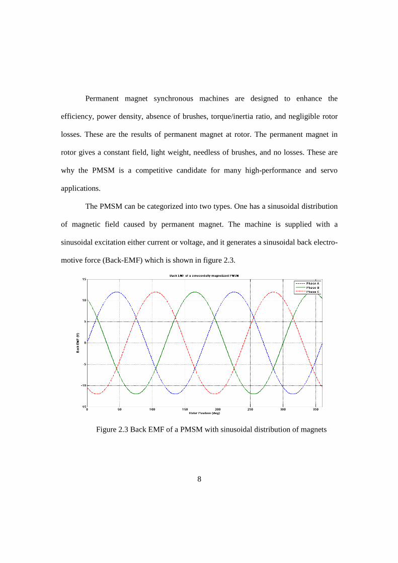
The PMSM can be categorized into two types. One has a sinusoidal distribution

of magnetic field caused by permanent magnet. The machine is supplied with a

sinusoidal excitation either current or voltage, and it generates a sinusoidal back electro-

motive force (Back-EMF) which is shown in figure 2.3.

Figure 2.3 Back EMF of a PMSM with sinusoidal distribution of magnets

9

The other type of PMSM has a radial polarization of the permanent magnets and

has a trapezoidal back-EMF as depicted in figure 2.4. This type of PMSM needs to be

fed by quasi-rectangular shaped currents into the machine.

Figure 2.4 Back EMF of a PMSM with radial magnetization

The PMSM is constructed with two major parts, stator and rotor, as shown in

figure 2.5.

Figure 2.5 Structure of stator and rotor for 3-phase PMSM

10

Figure 2.5 shows a 12 stator slots and a rotor constructed with laminated iron

sheets. The structure of stator and rotor is punched with laminated iron core because of

reducing eddy current losses in stator and rotor. From the rotor structure, there are two

different ways to place permanent magnets on the rotor. Based on placement, the

PMSM can be classified into two groups. They are called surface mount permanent

magnet synchronous motors (SPMSM) and interior permanent magnet synchronous

motors (IPMSM). Figure 2.6 depicts the cross-section of SPMSM and IPMSM with the

position of permanent magnet.

(a) (b)

Figure 2.6 Cross section of permanent magnet synchronous motor (a) Surface mount permanent magnet synchronous motor (b) Interior permanent magnet synchronous motor

11

The first group is called surface mount permanent magnet synchronous motor

(SPMSM). The permanent magnet is placed on the surface of the rotor. SPMSM is easy

to build owing to the ease of magnet mounting. Moreover, the configuration is usually

utilized for low speed applications and low torque response. The magnetic material on

the surface of the rotor affects the flux distribution in the airgap because the

permeability of the permanent magnet is almost unity, which is closed to the air

permeability. When the current is injected into the stator winding, the stator flux is

generated and reacted with the flux from permanent magnet of the rotor. As a result, the

electromagnetic torque acting on the shaft is produced. Figure 2.7 demonstrates the

rotor shaft for 4-pole, 3-phase SPMSM, which has the permanent magnet mounted on

the surface of the rotor.

Figure 2.7 Structure of 4-poles rotor with permanent magnet at the surface

The other group is named interior permanent magnet synchronous motor

(IPMSM). IPMSM contains permanent magnets embedded inside the rotor as show in

12

figure 2.8. This geometric difference alters the IPMSM’s characteristics. In fact,

IPMSM is suitable for high speed operations. Furthermore, because of the permanent

magnet mounted inside the rotor, it has more robust permeability and relatively larger

magnetizing inductance since the effective airgap being low. The armature reaction

effect is dominant, and therefore IPMSM is possible to be controlled in the constant-

torque and the constant-power flux-weakening. Moreover, a saliency is introduced in

the machine (Lq > Ld, which is discussed in section 2.3), and as a result, the torque is

contributed by field as well as reluctance effect.

Figure 2.8 Structure of interior permanent magnet synchronous motor (IPMSM)

2.3 Modeling of PMSM

2.3.1. The definition of rotor velocity and position in PMSM

In electrical motor, there are electrical and mechanical values for rotor velocity

and position. For instance, mechanical rotor position corresponds to the actual position

13

of the shaft during rotation. Consequently the time necessary for 360 degrees of

mechanical rotation is referred to as mechanical cycle. On the other hand, an electrical

cycle is the rotation of electromagnetic field around the airgap For example, figure 2.9

demonstrates a 3 phases, 4 pole permanent magnet synchronous motor. As can be seen,

if the rotor shaft rotates 180 mechanical degrees (a half mechanical cycle), the electrical

position of the rotor rotates 360 electrical degrees (one electrical cycle). From this

statement, the relationship between electrical position and mechanical position can be

concluded in equation 2.2.

Figure 2.9 Simplified structure of 3 phases, 4 poles permanent magnet synchronous motor

�� � · �� (2.2)

14

where �� , �� �� � denote the electrical rotor position, the mechanical rotor

position, and the number of rotor poles, respectively.

In the same manner, the rotor velocity can be represented by equation 2.3,

which is based on equation 2.2 (� � ��� �).

�� � · �� (2.3)

where �� , �� �� � denote the electrical rotor velocity, the mechanical

rotor velocity, and the number of poles, respectively.

2.3.2 Electromechanical Description

PMSMs with non-sinusoidal rotor field have been held responsible for

producing torque ripple on the shaft of the motor [26]. This could be a significant

drawback, especially for servo applications. Over the last two decades, different

methods to reduce torque ripple in permanent magnet machines have been developed.

These methods can be divided into two different categories as following:

(a) Methods that are based on introducing a change in the design of the machines in

order to reduce torque ripple. Many different techniques have been introduced

and torque ripple can be greatly reduced at the cost of a more complex design

and, thus, a more expensive machine.

(b) Methods that are based on controlling current so that the torque ripple is

cancelled out. A variety of methods have evolved using different techniques to

achieve the goal. In the mitigation of torque ripple, methods typically rely on a

detailed knowledge of the machine. This is accomplished by schemes that

15

identify the parameters of the machine during startup and also during operation

[25] or adaptive control of current [26].

Traditional analysis of permanent magnet synchronous machines has been based

on an analytical relationship between the q- and d-axis stator current (or voltage) and

the electromagnetic force created to establish motion (torque). The following two

subsections introduce the electrical equivalent circuit for each phase of the PMSM,

present equations for torque and also establish the significance of accurate estimation of

flux linking each phase of the stator.

There are three basic components to the model of an electromechanical device -

the voltage equation, the flux linkage equation and the torque equation. The equivalent

circuit of the machine can be described as a series combination of the coil resistance,

inductance of the winding and the back-emf due to the rotor speed and induced flux.

Figure 2.10 shows this equivalent circuit.

Su

mω

SR

e

SL

Figure 2.10 Equivalent circuit model for phase winding of the PMSM.

Accordingly, the voltage equation of the series circuit is defined as the algebraic

sum of the ohmic drop and the rate of change of flux linkage (Faraday’s law) given by

equation 2.4 and it is including the effect of back motional EMF.

16

Figure 2.11 The simplified PMSM in term of 3-phase space vectors

Figure 2.11 shows the state space model of a 3-phase system. In order to

simplify the 3-phase system to 2-phase system, Park’s transformation to put everything

on the rotor is applied into the stator voltage, current, and flux linkage vectors as shown

in equation (2.4) – (2.6), and they are on the stator reference frame.

���������� � � ������ � · ����� � · � ���� � !" � #!$ (2.4)

%�������� � � �&���� � · &���� � · & ���� � '" � #'$ (2.5)

(��������� � � �(���� � · (���� � · ( ���� � Ψ" � #Ψ$ (2.6)

Where a denotes an unit vector and the argument is equal to *+,-. . In addition,

� , & , �� ( denote phase voltage, current, and flux linkage, respectively. In those

equations, the superscript “(S)” denotes the stator reference frame. Therefore, the next

step is to transform the stator reference frame to the rotor reference frame. In order to

easily depict the transformation, figure 2.12 is shown the space vectors in stator and

rotor reference frame in PMSM.

of PMSM, the stator voltage is shown in equation (2.7).

����������where; (���������Then; ����������

/� , 0� , �� , ��, ��inductance, electrical angle position of rotor, electri

constant flux rotor from permanent magnet, respectively.

Figure 2.12 The space vector of stator and rotor reference frame in PMSM[The superscript “(R)” denote

17

frame in PMSM. From the figure 2.12 and the equivalent circuit model

the stator voltage is shown in equation (2.7).

�� � � /� · %�������� � ��� (���������

�� � � 0� · %�������� � Ψ� · *+12

�� � � /� · %�������� � 0� · ��� %�������� � #��Ψ3

�� � denote the stator winding resistance, stator winding

inductance, electrical angle position of rotor, electrical angle velocity of rotor, and

constant flux rotor from permanent magnet, respectively.

Figure 2.12 The space vector of stator and rotor reference frame in PMSMhe superscript “(R)” denotes the rotor reference frame (d-q axis)

quivalent circuit model

(2.7)

(2.8)

*+12 (2.9)

denote the stator winding resistance, stator winding

cal angle velocity of rotor, and

Figure 2.12 The space vector of stator and rotor reference frame in PMSM q axis).]

18

As shown in figure 2.12, the relationship between stator and rotor reference

frame is as:

�����4���� � ���������� · *5+12 (2.10)

%���4���� � %�������� · *5+12 (2.11)

Therefore, the equation (2.9) can be rewritten in rotor reference frame as

equation (2.12).

�����4���� � /� · %���4���� � 0� · ��� %���4���� � #��0�%���4���� � #��Ψ3 (2.12)

From equation (2.12), it can be divided into real and imaginary term as shown in

equation (2.13) – (2.15).

�����4���� � !� � #!6 (2.13)

!� � /� · &� � 0� · ��� &� 7 0���&6 (2.14)

!6 � /� · &6 � 0� · ��� &6 7 0���&� � ��Ψ� (2.15)

The output mechanical torque generated ‘89’ in a synchronous machine is

related to the mechanical speed ‘ωm’ at the steady state as given by equation (2.16).

89 � !�'� � !�'� � ! ' �� (2.16)

Further, the equation for motion of PMSM is given by equation (2.17).

89 7 8: � ; ��� ����� � ��� (2.17)

19

Where 89 , 8: , ; , �� � denote mechanical torque (generated), mechanical

load torque, moment of inertia, and friction, respectively.

Moreover, the equation for electrical torque in a PMSM at the steady state can

be written in term of magnetizing flux and stator phase currents on the rotor reference

frame as shown in equation (2.18).

8< � 32 �2 ?Ψ�'6 � @0� 7 06A'6'�B (2.18)

As discussed in section 2.2.1, the SPMSM is a non-salient machine (0� � 06),

but the IPMSM is a magnetically salient machines@06 C 0�A. Therefore, if the

machine is a surface mount permanent magnet synchronous motor, the electrical torque

is finally shown in equation (3.11).

89 � � Ψ�'6 (2.19)

In the equation (2.17), Ignoring the dynamic friction of the system, the block

diagram of SPMSM on the rotor reference frame can be shown in figure 2.13 by using

equation (2.4) - (3.11) [24].

Figure 2.13 Block diagram of SPMSM on the rotor reference frame

[D� [D�

2.4

The acoustic noise and vibration in PMSM are caused by two major categories

of force, namely tangential and ra

stator frame along in ra

acting on the shaft (and components that are in tandem with the shaft) in the PMSM. In

order to clarify the concept of vibration and force, those radial and tangential f

need to be discussed.

Radial forces cause the

forces are the unwanted byproducts of the electromechanical energy conversion

the direction of the radial

Its direction is in the normal direction

20

Figure 2.13 Block diagram of SPMSM on the rotor reference frame

� is the electrical time constant, and it is equal to

� is the mechanical time constant, and it is equal to

Force and Torque Distribution in PMSM

The acoustic noise and vibration in PMSM are caused by two major categories

force, namely tangential and radial. While radial vibration causes vibration of the

stator frame along in radial direction, the tangential vibration generates pulsations

acting on the shaft (and components that are in tandem with the shaft) in the PMSM. In

order to clarify the concept of vibration and force, those radial and tangential f

cause the radial vibration of the machines. Consequently, these

byproducts of the electromechanical energy conversion

radial forces is perpendicular to that of the rotation of the machine.

Its direction is in the normal direction (90o apart from tangential)

Figure 2.13 Block diagram of SPMSM on the rotor reference frame

is the electrical time constant, and it is equal to :E4E ]

anical time constant, and it is equal to 1/J ]

The acoustic noise and vibration in PMSM are caused by two major categories

dial. While radial vibration causes vibration of the

dial direction, the tangential vibration generates pulsations

acting on the shaft (and components that are in tandem with the shaft) in the PMSM. In

order to clarify the concept of vibration and force, those radial and tangential forces

vibration of the machines. Consequently, these

byproducts of the electromechanical energy conversion. In fact,

rotation of the machine.

apart from tangential) of the rotor and

21

producing unwanted radial vibration in the stator frame. These forces are local vector

quantities that have different effects on different parts of the machine. To the contrary,

the tangential component of force in terms of torque is mostly responsible for the

motion and is a component that needs to be controlled precisely. However, when the

machine is operated, it cannot avoid having the radial forces acting on the rotor and

stator frames. Using Maxwell stress method distribution of the radial and tangential

force densities in the airgap of the machine can be expressed as equations 2.20 and 2.21,

respectively.

FG � 12 · �I · ��G 7 ��� (2.20)

F� � 1�I · @�G · �� A (2.21)

Where 0and,,,, µtntn BBff denote normal and tangential component of the

force density in airgap, normal component of flux density, tangential component of flux

density, and absolute permeability, respectively.

The electromagnetic torque of PMSM is generated by the tangential forces

acting on the rotor. In fact, the tangential force is dependent upon the distribution of the

magnetic field in the airgap. The tangential forces are also produced on the stator poles

and cause unwanted vibrations in the stator frame. Therefore, mitigation of acoustic

noise and vibration includes influencing not only the normal, but also the tangential

forces. These forces are generating the electromagnetic torque on the rotor and

22

tangential vibration of the stator frame. However, some significant conditions need to

be considered, regarding force distribution in electromagnetic devices.

First of all, the magnetic field density and magnetic energy inside the

unsaturated ferromagnetic material are very small. Therefore, the force contributions

from these components are very small. Moreover, the relative permeability of

permanent magnet is very close to unity. The force distribution in the air and PM are

therefore identical for the same position if the points that are probed are close.

Next, radial forces throughout any component exhibit different magnitudes at

different points. Therefore, compensation cannot always be based on the average values

measured in the machine. Local effects need to be taken into account. In addition, local

saturation is observed at pole tips owing to a large concentration of flux. This causes a

much larger force at the tip of the stator poles than the rest of the pole. At the surface of

a material with high permeability, the tangential component of flux density is almost

equal to zero, and the normal force density almost entirely depends on normal

component of flux density. On the other hand, the tangential component of force is

almost zero at the surface of high permeable material for the same reason.

Finally, from an energy’s point of view, almost all the energy exchange happens

at the iron-air interface as the system moves [20]. In fact, a region with highest energy

density is replaced by a region with almost zero energy density, as such the highest rate

of energy change with incremental displacement happens at the interface of iron and air,

and thus almost all the force as the normal component produces on the surface of the

23

iron toward the air.

2.4.1 Fields and Forces at the interface between two materials

In this section, the analysis of fields and forces between two materials acting

inside the machines are considered. The theory of continuity [22] plays a key role in

explaining the distribution of tangential and normal field and force components. The

field and force components can be considered in two parts, including tangential (the

same direction with rotating direction) and normal (90o apart from rotation direction).

The field density and field intensity at the interface between materials having different

permeability are given in accordance with continuity theorem in equations 2.22 and

2.23. However, zero surface current densities at the surface of the stator pole7airgap

interface7needs to be assumed.

airnMn BB ,19, = (2.22)

19,, Mtairt HH = (2.23)

Equation 2.23 given above can be expresses in terms of permeability as

19,,19,

19

19,,

MrairtMt

M

Mt

air

airt

BB

BB

µ

µµ

=

=

(2.24)

From equation 2.24, we see that the tangential component of field density at the

interface of two materials with different permeability is not continuous. Since the

permeability of M-19 is of the order of 105, the tangential field density inside the iron is

24

much greater than that present in the air outside it. To assess the influence of these

components on the force generated at that surface, we consider the tangential

component of force given by the equation

ntt BHf = (2.25)

airnairtair

airt BBf ,,,

1

µ=

(2.26)

19,19,19

19,

1MnMt

MMt BBf

µ=

(2.27)

Using the expressions for Bn, M19 and Bt, M19 from equations 2.22 and 2.24

respectively in equation 2.28, tangential force component in M-19 is given by

airnairtMt BBf ,,0

19,

1

µ=

(2.28)

At the air- M19 interface, the tangential component of flux density in the air is

almost zero. Therefore, with this information, it can be observed from equations 2.26

and 2.28 that the magnitude of tangential component of force inside and outside the iron

is very negligible when it is compared to the normal components. In the iron- air

interface, it can be seen that the tangential force present inside the iron is almost zero.

On the other hand, the normal component of force at the interface is given as following:

25

2,

0

2,

2,

0, 2

1)(

2

1airnairtairnairn BBBf

µµ≈−=

(2.29)

219,

0

219,

219,

019, 2

1)(

2

1MnMtMnMn BBBf

µµ≈−=

(2.30)

This is a very large value since the magnitude of �G is unchanged in either case.

Therefore, the investigation of the field a component at the interface indicates that

tangential component of the field in the air-side of the interface is significantly smaller

than the normal component. Therefore, it can be said that the forces on a conducting

body with no surface current density are produced on the surface of iron as the normal

force component. In fact, the normal force component is directed toward the air, and it

is higher where the surface flux density is higher. If this normal force happens to be in

the same direction of rotating motion, it is viewed as a useful result of the

electromechanical energy conversion. Otherwise, it is viewed as a troublesome by

product that causes noise, vibration, and deformation. The higher the normal surface

force in the direction of movement and lower on other directions, the more efficient

energy conversion process is resulted.

2.5 PMSM Drive Setup

There can be divided the PMSM drive setup into four major parts, including

motor, generator, loads, and torque meter parts. Figure 2.14 shows the experimental

setup.

26

TorqueM PMSM

Differential Torque Meter

Computer

Speed

KollMarganBLDC Drive

Controller

Operated asGenerator

Load(Balanced/

Unbalanced)

, ,a b ci i i

Figure 2.14 System demonstrating the experimental setup

In this work, PMSM is driven by a brushless direct current motor drive system

(BLDC Drive). The BLDC system is controlled by programmable controls, named as

KollMorgan drive system. This work is setup to utilize the KollMorgan drive system to

operate in “motoring mode.” Figure 2.15 shows the KollMorgan system that is used in

the laboratory.

27

Figure 2.15 KollMorgan system in REVT laboratory

Figure 2.16 The 3-phase, 4 poles permanent magnet synchronous motor

28

The next part is the PMSM. The PMSM is operated in “generating mode.”

BLDC is programmed to drive the PMSM, and the balanced and unbalanced loads are

applied to the 3-phase voltage terminals of PMSM. Figure 2.16 shows the PMSM that is

employed in the experimental setup.

In this setup, resistive loads are applied to the PMSM’s terminals. There are

both balanced and unbalanced loads to demonstrate the cogging torque both balanced

and unbalanced three-phase currents. The three-phase current profiles is utilized in the

field reconstruction method (FRM) in MATLAB program to compute the torque. Then

the FRM’s torque calculation is compared with the torque from BLDC. This will be

discussed in chapter 4. Figure 2.17 demonstrates the resistant loads that are used in this

experimental setup.

Figure 2.17 Demonstrating resistant loads in experimental setup

29

The other part of the system is a torque meter. This torque meter is a differential

torque meter, which means at the steady state the output of the torque meter is equal to

zero. Figure 2.18 shows the torque meter in this setup.

Figure 2.18 Differential torque meter

30

CHAPTER 3

FORCE CALCULATION AND FIELD RECONSTRUCTION METHOD

The force calculation of PMSM has been proposed on several levels. For

instance, field oriented control technique (FOC) for PMSM is based on the assumption

of a purely sinusoidal back electromotive force (back-EMF). In this technique, the

three-phase currents are transformed from 3-axis to 2-axis system on stator reference

frame. Thereto, 2-axis currents are metamorphosed from stator reference frame to rotor

reference frame at steady state, which are DC terms. This method gives a good result of

force calculation. Nevertheless, it is time consuming [20]-[21].

Another technique is direct torque control technique (DTC) [2]. Based on this

idea, the force calculation is computed on stator reference frame, and the 2-axis currents

have still been used. However, the problem is stator fluxes, including direct axis and

quadrature axis components of flux, in AC terms. These stator fluxes are included an

integral part of calculation, which is added to previous error in every single calculation.

Consequently, the stator fluxes are draft until they are saturated.

As a result, many researchers have proposed several methods to calculate the

force [17]-[19]. In addition, the method is computational time and precision.

Remarkably, numerical methods are seemingly suitable for force computation [20]-[21].

31

3.1 Force Calculations

The calculations of electromagnetic force can be viewed as the main part of

simulating the electromechanical energy conversion process. So far many numerical

methods and formulations for force calculation have been proposed, such as finite

element analysis (FEA), finite difference method (FDM), magnetic equivalent circuit

(MEC), Fourier series method (FSM), and some global or local variation and mapping

techniques. They all are based on approximations of the electromagnetic fields and

stored magnetic energy in the machine. All of the above methods, because of flexibility,

ease of modeling and post processing, finite element analysis, FEA, has evidently been

a good candidate and employed to efficiently compute the electromagnetic force.

Along those lines, electromagnetic force can be computed by the virtue of the

Maxwell Stress Tensor (MST), which is one of the numerical methods and based on

FEA. Necessary calculations of electromagnetic forces acting on the stator and rotor are

presented in the literature [18]-[19]. In order to perform the analysis, the following

assumptions have been setup:

• Surface mounted magnets on the rotor of the PMSM are uniformly

magnetized.

• Influence of eddy and hysteresis currents is negligible.

• The stator is slot-less with 8 independent stator phases distributed

around a uniform airgap.

• Operation under saturation is not allowed.

32

The majority of the energy conversion takes place in the airgap. The tangential

and radial components of force density in the airgap can be expressed using equation

(3.1)-(3.2), and they also represent the basis for an investigation of the force production

within the machine.

F� � JKL�MNMO� (3.1)

FG � J,KL@MN,5 MO,A (3.2)

where FG , F� , �G, �� �� �P denote normal and tangential component of the

force density in airgap, normal and tangential component of flux density, and absolute

permeability respectively.

3.2 Field Reconstruction Method (FRM)

In the electromechanical energy conversion (EMEC), it is very important to

obtain the flux density distribution, so is the field reconstruction method (FRM). Figure

3.1 shows a block diagram representation of field reconstruction method [20]-[21].

ecba andiii θ,,, tn BB ,

Figure 3.1 Demonstration of field reconstruction method

33

As seen in figure 3.1, FRM needsthe input of three-phase current profiles and

rotor position in order to calculate the flux density distribution.

In order to efficiently design FRM and the machine, simulation is first needed to

be done before designing the machine. In fact, the finite element analysis (FEA) is

utilized in the simulation. In this particular approach, commercially available software-

Magnet® by Infolytica was used. For a complete simulation of the 3-phase permanent

magnet synchronous machine, there are four basic inputs. They include three phase

currents and mechanical speed of the rotor. The resultant normal and tangential

components of flux density in the airgap for any rotor position were obtained from the

FEA solution. Corresponding force densities were calculated using Maxwell Stress

Tensor method as described in equations (3.1) and (3.2). For obtaining the solution, a 2-

dimensional cross section was used, as shown in figure 3.2.Figure 3.3 shows the 3-

dimensional finite element model of the PMSM used for the modeling.

34

Figure 3.2 Representation of 2-Dimensional model of the PM machine used for field reconstruction.

Figure 3.3 Demonstration of 3-Dimensional model of the PM machine modeled using Finite Element Analysis.

35

The majority of energy conversion takes place in the airgap as shown in figure

3.4. A field reconstruction method (FRM) is proposed to compute the electromagnetic

torque and radial forces of PMSM. The FRM utilizes the three phase current profile and

rotor position, as shown in figure 3.4, to calculate radial and tangential component of

the force density and the flux density. Furthermore, FRM can predict torque ripple

which is affected by geometry of the machine. Stator slots play a central role in the

profile torque ripple when there is no stator excitation, known as cogging torque.

aiur

biur

ciur

rθ

{ }, ,n t zF F F F = ur

{ }, ,n t zB B B B = ur

Figure 3.4 Block diagram of field reconstruction method

As can be noted from figure 3.4, using an appropriate integration contour around

the stator and rotor, the actual force acting at each surface can be computed by

integrating the force density components over the respective surface area as follows:

Q� � R F������S� (3.3)

QG � T R UFG�V�WP (3.4)

36

where X, T, U �� V� represent surface area of integration, stack length of the

machine (along the Z-direction), radius of the integrating contour, and angle component

in cylindrical system of coordinates respectively.

Using equation (3.3)-(3.4), the electromagnetic torque can be calculated as

shown in equation (3.5). As a result, these computations can be used to mitigate torque

pulsation and the vibration in the stator frame.

Y � R @U� Z F�����A · �������� (3.5)

Figure 3.5 illustrates the distribution of the magnetic flux density in a 3-phase

PMSM due to three phases’ excitation of the stator winding.

Figure 3.5 Distribution of magnetic flux density in a 3-phase PMSM

37

It is shown in figure 3.5 that each conductor on the stator contributes to the

tangential and radial components of the flux density in the airgap. Any change in the

geometry within PMSM can alter the tangential and components of the flux density that

are constituted by a conductor located at V�[ as shown in equation (3.6).

��,[ � ���&[� · \��V� 7 V�[� ; 0 ^ �_ ^ ,-̀

�G,[ � �G�&[� · \G�V� 7 V�[� (3.6)

where �, ��, �G, \� �� \G denote number of magnetic pole pairs, scaling

function representing the dependency of the tangential and radial flux density upon the

current magnitude, and impact of the geometry (one conductor) respectively. Also, V�[

represents the location of the a�b conductor carrying a current of &[.

The resultant tangential and radial components of the flux density in the airgap

for any given rotor position can be expressed by using superposition (including the

contributions from the permanent magnets) theory and a truncated generalized Fourier

series as shown in equation (3.7)-(3.8). These expressions portray an elegant illustration

of the separation between factors influenced by the structure of the machines

�\� �� \G� and external excitation@��,[ �� �G,[A.

���V�, &c, … , &�� � ��,e� � ∑ ��,[�&[� · \��V� 7 V�[��[gc (3.7)

�G�V�, &c, … , &�� � �G,e� � ∑ �G,[�&[� · \G�V� 7 V�[��[gc (3.8)

38

Equation (3.1) and (3.2) can therefore be rewritten by using the tangential and

radial components of the force densities as follows:

F��V�, &c, … , &�� � JKLhMO�iE,jJ,…,jk� · MN�iE,jJ,…,jk�l (3.9)

FG�V� , &c, … , &�� � J,KLmMN,�iE,jJ,…,jk� 5MO,�iE,jJ,…,jk�n (3.10)

In the same manner, equation (3.3) and (3.4) can also be rewritten to calculate

the force density over the outer surface of a cylinder, which is located in the middle of

the airgap, for each rotor position as shown in equation (3.11)-(3.12).

Q���_� � � · 0 · / o F��V�, &c, … , &���V�,-̀P (3.11)

QG��_� � � · 0 · / o FG�V�, &c, … , &���V�,-̀P (3.12)

where �, 0, �� / denote rotor position, stack length of the machines and radius

of the integration surface respectively.

Seemingly, FRM contains key functions in equation (3.7) and (3.8), \� �� \G,

which are known as the basis functions. The basis functions have played a significant

role in the formulation of the field reconstruction method. In equation (3.13)-(3.14),

under unsaturated condition, FRM can calculate the distribution of field and force for at

any given position due to stator currents when the pattern of excitation is known, and

basis functions are identified. Also, the contributions of the permanent magnets will be

adjusted for the new rotor position.

��,[�&[� � �� · &[ (3.13)

�G,[�&[� � �G · &[ (3.14)

39

From equations (3.13) and (3.14), if the pattern of stator current excitation is

known, and flux density distribution is also calculated from the basis functions, which

are identified. As a result, equations (3.7) through (3.9) can be identified the distribution

of field/force for any given position. It must be noted that the contribution of the

permanent magnets are assumed as given. The basis functions ht and hn are an

unsaturated slot-less and have characteristics as following:

• ht has an even symmetry with respect to φs

• hn has an odd symmetry with respect to φs.

• Periodic with respect to φs,

Since the rotor has constant field from permanent magnet (without rotor

excitation), the resultant tangential force is, therefore, an odd function resulting in zero

average torque at every given point. Nevertheless, the radial forces exist even without

any magnetic source on the rotor. Figure 3.6 shows the tangential and normal

components of field density in the PM machine without load.

Figure 3.6 Tangential and radial flux densities in airgap generated by permanent magnets

40

It can also be seen that radial component of flux density in a PMSM is primarily

dominated by the field of the permanent magnet. Moreover, the normal component of

force density yields a nonzero average and dominated by the normal component of the

flux density even though it is without applying the stator current. Therefore, radial

forces, which are viewed as byproduct in electromechanical energy conversion process,

are significantly larger than their tangential counterparts. It is also important to note that

the tangential component of the flux density in the PMSM does not have a continuous

profile and only appears at distinct positions where the stator/rotor coils are located.

Integration of the tangential component of force density yields a zero average in the

absence of excitation, which indicates that there is not motion when no excitation is

applied.

From the above assumption, it must be noted that due to the periodic nature of

the basis functions, they can be expanded by using a Fourier series, i.e.:

\��V�� � \P� � ∑ \[� cos�aV��9[gc (3.15)

\G�V�� � \PG � ∑ \[G sin�aV��9[gc (3.16)

Where M denotes the selected truncation point that would provide satisfactory

precision. In the presence of saturation, the coefficients of the above series expansion

depend upon current.

In the simulation, since there is only one source of MMF in the machine during

the calculation of basis functions, the amount of time taken by FEA to compute this

“one-shot-result” is significantly lower than the time required for the simulation of the

41

complete system. Consequently, in practice FEA may not be suitable for the real time

torque ripple minimization because it is time consuming [20]. This advantage may

outstandingly prove that FRM is faster than FEA in real time control and more suitable.

It goes on to say that this method is not just for the reconstruction of sinusoidal

excitations. Since the current applied for the basis function is 1A, force calculation in

the machine for various optimized waveforms becomes extremely simple.

3.3 Basis Functions of Field Reconstruction Method

As known in section 3.2, the characterization of the “basis functions” is a key

function of field reconstruction method. As expressed in figure 3.7, the algorithm of

field reconstruction involves a flow chart of calculation and a meticulous analysis of

magnetic field distribution throughout the machine. In order to achieve this objective,

unit dc current is applied to one of the phases and the resultant flux distribution is

recorded. Using the inherent symmetry of the machine, this distribution can be rotated

in space to establish the effect of current in each conductor of the machine. Finally, the

field density distribution is obtained from the cumulative effect of current through the

stator windings, and the permanent magnets gives the overall estimate of flux over the

entire machine.

42

Figure 3.7 Demonstration of flow chart for field reconstruction method.

43

CHAPTER 4

EXPERIMENTAL RESULTS

In many applications, such as naval, automotive, and military, there are several

requirements of operation. In fact, quiet and torque pulsation free (radial and tangential

vibration) are desired. One of the major causes that generate sound, acoustic noise and

vibration is torque pulsation. In addition, magnitude and frequency of the torque ripple

is influenced by the magnetic design (cogging torque), geometry of the machine

(number of stator slots), and excitation. In this work, a 1-hp, 3-phase, 4 poles, 12 stator

slots PMSM has been used for simulation and experimental verification. In the

simulation, the Matlab/simulink program is used to calculate the torque using FRM. In

the experiment, PMSM is operated in generating mode by using a fully controllable

BLDC drive system as shown in figure 2.14. Then sets of balanced and unbalanced

loads are connected to the terminals of PMSM. The 3-phase load currents is measured

and used in the field reconstruction program in Matlab/simulink program.

4.1 Permanent Magnet Synchronous Motor

It is important to note that the surface mounted permanent magnets are radially

magnetized. Consequently, back-EMF of this machine is trapezoidal. The first

experiment that has been done is to test the PMSM, and the easiest way to accomplish

44

this is to Run the PMSM with no stator current at a fixed speed and measure the back-

EMF. In the simulation of this PMSM, FEA was used, and the magnitude of back-EMF

voltage from the machine is about 12.4 volts at the speed of 1000 rpm. Figure 4.1 shows

the result of back-EMF from FEA. In fact, the back-EMF is the trapezoidal waveform,

and it has the magnitude of 12.4 volts. In case of comparison with an actual PMSM,

figure 4.2 to figure 4.4 are the results of back-EMF at different speeds. In figure 4.2, the

corresponding experimental measurement shows a measurement of back-EMF of 12.4

volts.

Figure 4.1 Back-EMF of PMSM at 1000 rpm from FEA

Figure 4.2 Back-EMF of PMSM at 1000 rpm from PMSM

45

Figure 4.3 Back-EMF of PMSM 500 rpm from PMSM

Figure 4.4 Back-EMF of PMSM 1500 rpm from PMSM

4.2 Prediction of Electromagnetic Torque

The experimental system may be divided into two main parts, which are PMSM

(operating in generating mode) and KollMorgan drive (operating in motoring mode and

acting as a prime mover). When The three phase terminals of the PMSM is connected to

46

the sets of balanced and unbalanced load, the recorded three-phase current is injected

into the FRM in Matlab/simulink in order to calculate the torque of PMSM. Then the

torque of PMSM is compared with the torque of the prime mover. This comparison

demonstrates an a excellent match in terms of frequency and magnitude of the average

torque. At steady state it is expected that the inline torque meter will show a zero

average torque.

The electromagnetic torque of PMSM is computed by supplying the three-

current current profiles and rotor position into Matlab/simulink program However,

calculation of the torque stemming from the prime mover need to be done separately. In

fact, the torque needs to be computed in Excel program by using three-phase stator

current profiles, and then the currents are transformed into the rotor reference frame. As

known, the quadrature axis current on the rotor reference frame Is linearly proportional

to the torque of the machine, and the direct axis current on the rotor reference frame

creates the magnetizing flux. As a result, after the quadrature axis current is calculated,

the current value has to be calibrated into the unit of torque (Nm).

4.2.1 Calculation of quadrature axis current on rotor reference frame

In order to calculate the quadrature axis current on the rotor reference frame, the

three-phase current profiles of KollMorgan must be measured, and they are on the stator

reference frame. Therefore, three-phase system has to be simplified to two-phase

47

T ande r

ω

system by the use of Clarke’s transformation. Figure 4.5 shows the three-phase current

system.

Figure 4.5 Three-phase current vectors on stator reference frame (α-β axis)

The transformation equation can be expressed as

F"$I � u� · F�� � (4.1)

where f represents either voltage, current, flux linkage, or electric charge, and

u� � � · vwwwxcos �� cos y�� 7 W� z cos y�� 7 {W� zsin �� sin y�� 7 W� z sin y�� 7 {W� zc c c |}

}}~

Then the three-phase stator current of PMSM can be transformed into two-phase

system on stator reference frame as:

�&"&$&I� � u� · �&�&�&

� (4.2)

48

Now the three-phase system is transformed to two-phase system. The next step

would be a transformation from stator reference frame to rotor reference frame, so

called Park’s transformation. This calculation requires a vector rotation angle into

mathematical model to follow the rotor reference frame attached to the rotor flux.

The formula that is used to calculate and transform stator reference frame to

rotor reference frame is shown as:

�&�&6� � � cos �_ sin �_7 sin �_ cos �_� · �&"&$� (4.3)

where �_ is the rotor angle position.

4.3 Simulation and Experimental Results

There are sets of balanced and unbalanced loads at different speeds of rotor.

4.3.1 Operation under balanced loads condition

Figure 4.6 shows the three-phase balanced current of PMSM that is supplied to

the loads at 167 rpm.

Figure 4.6 Three-phase current supplied to the load of PMSM at 167 rpm

49

Figure 4.7 Comparative results of torque between KollMorgan and PMSM using FRM at 167 rpm under balanced load condition

Figure 4.7 shows the torque between prime mover and PMSM. The PMSM’s

torque is the results of a half cycle of three-phase stator current. This is because of the

limitation of sampling data of FRM in Matlab/simulink program that limits the

sampling of 10kHz from the captured data to be injected into the FRM program. That is

why FRM can only compute 3 cycles of torque. This result is matched with the targeted

PMSM, which has 12 stator slots. Moreover, the results between KollMorgan and FRM

are matched in both the average torque and the frequency.

0

0.1

0.2

0.3

0.4

0.5

0.6

0.7

-0.8

-0.6

-0.4

-0.2

0

PMSM’s torque from FRM

KollMorgan’s torque from calculation

Average = 0.52Nm

Average = 0.52Nm

50

Figure 4.8 Comparative results of torque between KollMorgan and PMSM using FRM at 334 rpm under balanced load condition

Balanced three-phase current (Generating mode) (A)

Torque ripple of KollMorgan (Motoring operation) (Nm)

Torque ripple of PMSM calculated by FRM (Nm)

Average = 0.7 Nm

Average = 0.7 Nm

51

Figure 4.8 shows an operation of PMSM at 334 rpm under balanced load

condition. A cycle of three-phase stator current of PMSM is injected into FRM program

to calculate the electromagnetic torque. Evidently, there are 6 periods of torque in one

period of current, which means there are 12 stator slots. More significantly, the

algebraic summation of PM’s torque and KollMorgan’s torque is approximately equal

to zero Nm.

4.3.2 Operation under unbalanced loads condition

Figure 4.9 and 4.10 shows an unbalanced three-phase current of PMSM

operating in generating mode, and the PMSM is run at 1000 rpm. The measured current

has three electrical cycles. As a result, the torque pulsation will have 36 pulses due to

the structure of PMSM (12 stator slot).

Figure 4.9 Unbalanced three-phase current of PMSM at 1000 rpm

Unbalanced three-phase current (Generating mode) (A)

52

Figure 4.10 Comparative results of torque between KollMorgan and PMSM using FRM at 1000 rpm under unbalanced load condition

Torque ripple of KollMorgan (Motoring operation) (Nm)

Torque ripple of PMSM calculated by FRM (Nm)

53

CHAPTER 5

CONCLUSIONS

In this research, a field reconstruction method (FRM) has been introduced and

implemented on Matlab/simulink program. In case of a real time vibration and acoustic

noise cancellation, the torque pulsations have to be calculated and predicted correctly.

Field reconstruction method has been presented for calculation of torque ripple.

The FRM allows for the reconstruction of the electromagnetic fields due to the phase

currents using basis functions that are obtained using a few snapshots of the magnetic

field distribution. To accurately calculate torque, the tangential and normal components

of magnetic field, need to be computed. As a result, FRM can correctly calculate the

torque of PMSM.

In experiment, the investigation shows that FRM can accurately calculate the

torque pulsation or cogging torque under both balanced and unbalanced operations

when compared with BLDC’s torque pulsation. Furthermore, the FRM can confirm the

effect of torque ripple due to the geometry of PMSM. In fact, a 12 stator slots PMSM

was studied, and the calculation was done by FRM. The resultant cogging torque

calculated by FRM shows the accurate calculation of the torque which is affected by

stator slot geometry.

54

Field reconstruction method is a new numerical technique for analysis and

design of a PMSM. This technique is suitable with a real-time control because it

consume less calculating time than FEA. Also, FRM combines ideas from

electromechanical energy conversion, signal reconstruction, and pattern recognition in

order to control and develop the machine efficiently.

55

APPENDIX A

EXPERIMENTAL TESTBED AND THE PMSM

56

Laminated stator and permanent magnet rotor

A 4 poles, 12 stator slots PMSM after winding

57

The permanent magnet synchronous motor

Experimental setup

58

REFERENCES

1. P. C. Krause, O. Wasynczuk, and S. D. Sudhoff, “Analysis of Electric Machinery and Drive Systems”, 2nd ed., John Wiley and Sons, Piscataway, N.J., pp. 191-274, 2002.

2. I. Takahashi, and T. Noguchi,“A New Quick-Response and High-Efficiency Control Strategy of an Induction Motor”, IEEE Transactions on Industrial Applications, Vol. IA-22, No. 5, pp. 495-502, 1986.

3. T. M. Jahns and W. L. Soong, “Pulsating torque minimization techniques for permanent magnet ac drives- A review”, IEEE Transactions on Industrial Electronics, vol. 43, pp. 321–330, Apr. 1996.

4. C. Studer, A. Keyhani, T. Sebastian, and S. K. Murthy, “Study of cogging torque in permanent magnet machines”, in Proc. IEEE 32nd Ind. Applications Soc. (IAS) Annual Meeting, vol. 1, Oct. 1997, pp. 42–49.

5. D. C. Hanselman, “Effect of skew, pole count and slot count on brushless motor radial force, cogging torque and back EMF,” Inst. Elect. Eng. Proc.—Elect. Power Appl., vol. 144, no. 5, pp. 325–330, Sep. 1997.

6. J. Y. Hung and Z. Ding, “Design of currents to reduce torque ripple in brushless permanent magnet motors”, Proc. Inst. Elect. Eng. B, vol. 140, no. 4, pp. 260-266, 1993.

7. D. C. Hanselman, “Minimum torque ripple, maximum efficiency excitation of brushless permanent magnet motors”, IEEE Transactions on Ind. Electronics, vol. 41, pp. 292–300, June 1994.

8. V. Petrovic, R. Ortega, A. M. Stankovic, and G. Tadmor, “Design and implementation of an adaptive controller for torque ripple minimization in PM synchronous motors”, IEEE Transactions on Power Electronics, vol. 15, pp. 871– 880, Sept. 2000.

9. T. S. Low, T. H. Lee, K. J. Tseng, and K. S. Lock, “Servo performance of A BLDC drive with instantaneous torque control”, IEEE Transactions on Industrial Applications, vol. 28, pp. 455–462, Apr. 1992.

10. N. Matsui, T. Makino, and H. Satoh, “Auto-compensation of torque ripple of direct drive motor by torque observer”, IEEE Transactions on Industrial Applications, vol. 29, pp. 187–194, Feb. 1993.

11. S. K. Chung, H. S. Kim, C. G. Kim, and M.-J. Youn, “A new instantaneous torque control of PM synchronous motor for high-performance directdrive applications”, IEEE Transactions on Power Electronics, vol. 13, pp. 388-400, May 1998.

59

12. F. Colamartino, C. Marchand, and A. Razek, “Torque ripple minimization in permanent magnet synchronous servo drive,” IEEE Transactions on Energy Conversion, vol. 14, pp. 616–621, Sept. 1999.

13. Q. Weizhe, S. K Panda, J. X. Xu, “Torque ripple minimization in PM synchronous motors using iterative learning control” , IEEE Transactions on Power Electronics, Volume 19, Issue 2, March 2004, pp. 272 – 279. 116

14. P. Zheng, J. Zhao, J. Han, J. Wang, Z. Yao, and R. Liu, “Optimization of the Magnetic Pole Shape of a Permanent-Magnet Synchronous Motor”, IEEE Transactions on Magnetics, Volume 43, Issue 6, June 2007, pp. 2531 – 2533.

15. A. Kioumarsi, M. Moallem, and B. Fahimi, “Mitigation of Torque Ripple in Interior Permanent Magnet Motors by Optimal Shape Design” IEEE Transactions on Magnetics, Volume 42, Issue 11, Nov. 2006, pp. 3706 – 3711.

16. J. Piotrowski, “Shaft Alignment Handbook”, New York: Marcel Dekker, 1995.

17. K. Komeza, A. Pelikant, J. Tegopoulos, S. Wiak, “Comparative computation of forces and torques of electromagnetic devices by means of different formulae”, IEEE Transactions on Magnetics, Volume 30, Issue 5, Part 2, Sep 1994, pp. 3475 – 3478.

18. W. Muller, “Comparison of different methods of force calculation”, IEEE Transactions on Magnetics, Vol. 26, No. 2, Mar 1990, pp. 1058-1061.

19. J. Mizia, K. Adamiak, A. R. Eastham, and G. E. Dawson, “Finite element force calculation: comparison of methods for electric machines”, IEEE Transactions on Magnetics, Vol. 24, Issue 1, Jan. 1988, pp.447 – 450.

20. W. Zhu, B. Fahimi, and S. Pekarek, “A Field Reconstruction Method for Optimal Excitation of Permanent Magnet Synchronous Machines”, IEEE Transactions on Energy Conversion, Vol.2, 2006.

21. A. Khoobroo, B. Fahimi, S. Pekarek, “A new field reconstruction method for permanent magnet synchronous machines”, IECON Int. Conf. on Ind. Electron. pp. 2009 – 2013, Nov 2008.

22. J. R. Melcher, Continuum Electromechanics, MIT Press, 1981. 23. A. B. Proca, A. Keyhani, A. El-Antably, W. Lu, and M. Dai, “Analytical

model for permanent magnet motors with surface mounted magnets”, IEEE Transaction on Energy Conversion, Volume 18, Issue 3, pp. 386–391, Sept. 2003.

24. Leonhard, W., Control of Electrical Drives, 3rd ed., Springler-Verlag, Berlin Heidelberg, pp. 12, 155-253, 2001

25. J. Holtz and L. Springob, “Identification and compensation of torque ripple in high precision permanent magnet motor drives," IEEE Transactions Ind. Application., vol. 43, no. 2, pp. 309-320, Feb. 1996.

26. V. Petrović, R. Ortega, A. M. Stanković, and G. Tadmor, “Design and implementation of an adaptive controller for torque ripple minimization in PM synchronous motors," IEEE Transactions on Power Electronics, vol. 15, no. 5, pp. 871 - 880, Sept. 2000.

60

BIOGRAPHICAL INFORMATION

Banharn Sutthiphornsombat was born on November 2, 1978 in Bangkok,

Thailand. He received his Bachelor of Science in Electrical Engineering from King

Mongkut’s Institute of Technology North Bangkok, Thailand, and Master of

Engineering in Electrical Engineering from King Mongkut’s University of Technology

Thonburi. His research interests include DC-DC converters, electrical motor drives,

power electronics, and renewable energy.