Previous Demand Elasticity Estimates ForAustralian Meat Products

Garry GriffithMeat, Dairy and Intensive Livestock Products Program,

NSW Agriculture, Armidale

Kym I’AnsonPreviously with the Industry Economics Sub-program,

Cooperative Research Centre for the Cattle and Beef Industry, Armidale

Debbie HillPreviously with the Industry Economics Sub-program,

Cooperative Research Centre for the Cattle and Beef Industry, Armidale

Roland LubettPreviously with the Industry Economics Sub-program,

Cooperative Research Centre for the Cattle and Beef Industry, Armidale

David VerePastures and Rangelands Program,

NSW Agriculture, Orange

Economic Research Report No. 5

January 2001

ii

NSW Agriculture 2001This publication is copyright. Except as permitted under the Copyright Act 1968, no part ofthe publication may be reproduced by any process, electronic or otherwise, without thespecific written permission of the copyright owner. Neither may information be storedelectronically in any way whatever without such permission.

ISSN 1442-9764

ISBN 0 7347 1264 2

Senior Author's Contact:Dr Garry Griffith, NSW Agriculture, Beef Industry Centre, University of New England,Armidale, 2351.

Telephone: (02) 6770 1826 Facsimile: (02) 6770 1830Email: garry.griffith@agric.nsw.gov.au

Citation:Griffith, G.R., I'Anson, K., Hill, D.J., Lubett, R. and Vere, D.T. (2001), Previous DemandElasticity Estimates for Australian Meat Products, Economic Research Report No. 5, NSWAgriculture, Orange.

iii

Previous Demand Elasticity Estimates ForAustralian Meat Products

Table of Contents

Page

List Of Tables ............................................................................................................................... iv

Acknowledgments ..........................................................................................................................v

Acronyms And Abbreviations Used In The Report....................................................................v

Executive Summary..................................................................................................................... vi

1. Introduction................................................................................................................................1

2. Previous Demand Elasticity Studies.........................................................................................32.1 Background ..................................................................................................................32.2 Domestic Retail Demand .............................................................................................3

2.2.1 Aggregated Retail Demand Analyses ..........................................................32.2.2 Disaggregated Retail Demand Analyses .....................................................6

2.3 Domestic Demand Analyses At Other Market Levels..............................................82.4 Export Demand Analyses ............................................................................................8

3. Comparison And Evaluation Of Previous Demand Elasticity Estimates ...........................10

4. Conclusions...............................................................................................................................12

5. References.................................................................................................................................13

iv

List of TablesPage

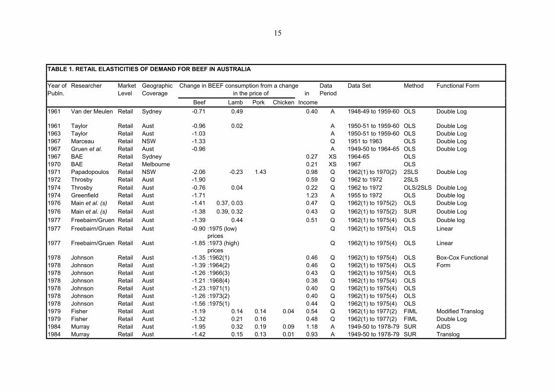
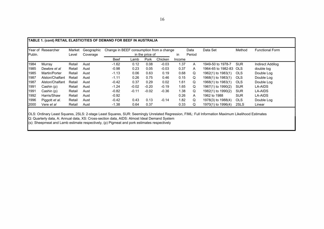
Table 1. Retail Elasticities of Demand for Beef in Australia 15

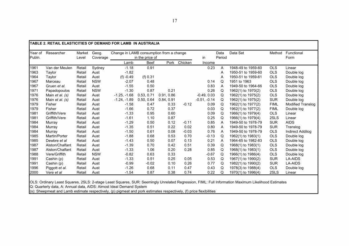
Table 2. Retail Elasticities of Demand for Lamb in Australia 17

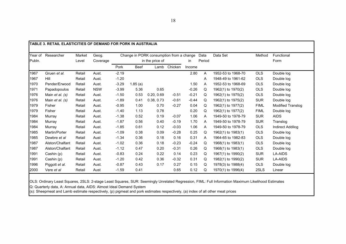
Table 3. Retail Elasticities of Demand for Pork in Australia 18

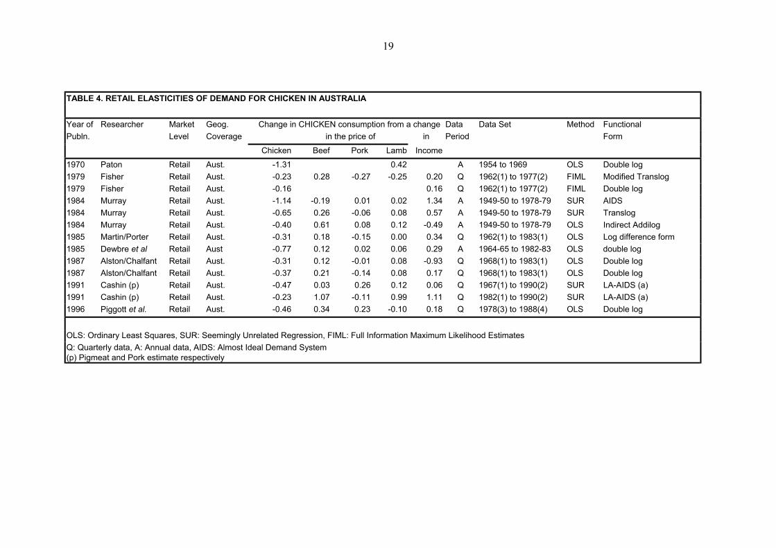
Table 4. Retail Elasticities of Demand for Chicken in Australia 19

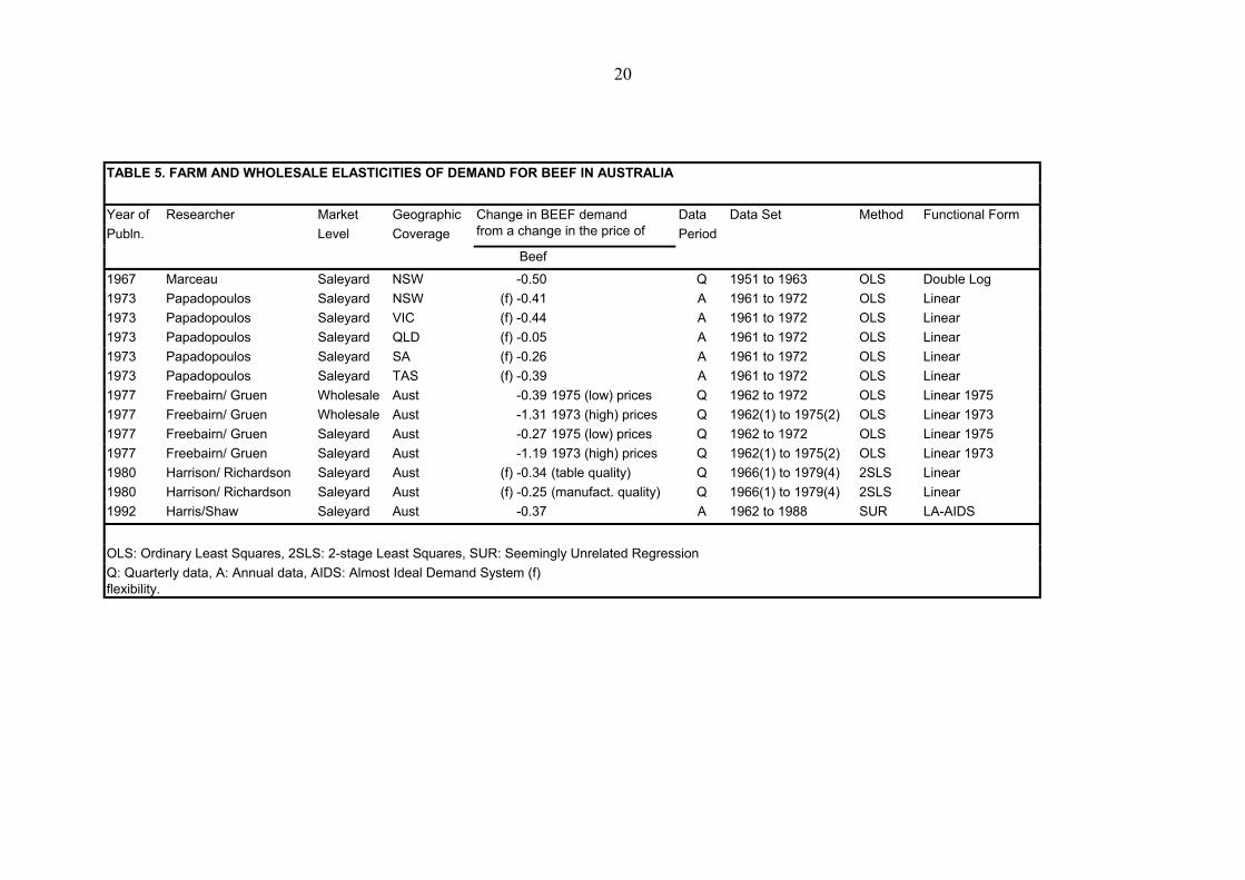
Table 5. Farm and Wholesale Elasticities of Demand for Beef in Australia 20

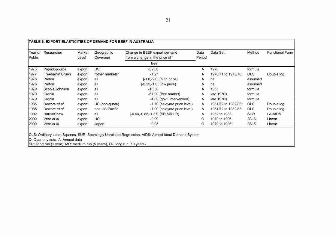
Table 6. Export Elasticities of Demand for Beef in Australia 21

v

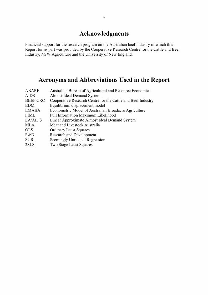
AcknowledgmentsFinancial support for the research program on the Australian beef industry of which thisReport forms part was provided by the Cooperative Research Centre for the Cattle and BeefIndustry, NSW Agriculture and the University of New England.

Acronyms and Abbreviations Used in the ReportABARE Australian Bureau of Agricultural and Resource EconomicsAIDS Almost Ideal Demand SystemBEEF CRC Cooperative Research Centre for the Cattle and Beef IndustryEDM Equilibrium displacement modelEMABA Econometric Model of Australian Broadacre AgricultureFIML Full Information Maximum LikelihoodLA/AIDS Linear Approximate Almost Ideal Demand SystemMLA Meat and Livestock AustraliaOLS Ordinary Least SquaresR&D Research and DevelopmentSUR Seemingly Unrelated Regression2SLS Two Stage Least Squares

vi

Previous Demand Elasticity Estimates For AustralianMeat Products

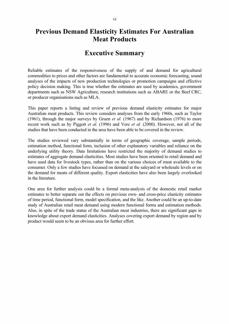
Executive Summary

Reliable estimates of the responsiveness of the supply of and demand for agriculturalcommodities to prices and other factors are fundamental to accurate economic forecasting, soundanalyses of the impacts of new production technologies or promotion campaigns and effectivepolicy decision making. This is true whether the estimates are used by academics, governmentdepartments such as NSW Agriculture, research institutions such as ABARE or the Beef CRC,or producer organisations such as MLA.

This paper reports a listing and review of previous demand elasticity estimates for majorAustralian meat products. This review considers analyses from the early 1960s, such as Taylor(1961), through the major surveys by Gruen et al. (1967) and by Richardson (1976) to morerecent work such as by Piggott et al. (1996) and Vere et al. (2000). However, not all of thestudies that have been conducted in the area have been able to be covered in the review.

The studies reviewed vary substantially in terms of geographic coverage, sample periods,estimation method, functional form, inclusion of other explanatory variables and reliance on theunderlying utility theory. Data limitations have restricted the majority of demand studies toestimates of aggregate demand elasticities. Most studies have been oriented to retail demand andhave used data for livestock types, rather than on the various choices of meat available to theconsumer. Only a few studies have focussed on demand at the saleyard or wholesale levels or onthe demand for meats of different quality. Export elasticities have also been largely overlookedin the literature.

One area for further analysis could be a formal meta-analysis of the domestic retail marketestimates to better separate out the effects on previous own- and cross-price elasticity estimatesof time period, functional form, model specification, and the like. Another could be an up-to-datestudy of Australian retail meat demand using modern functional forms and estimation methods.Also, in spite of the trade status of the Australian meat industries, there are significant gaps inknowledge about export demand elasticities. Analyses covering export demand by region and byproduct would seem to be an obvious area for further effort.

1

1 IntroductionReliable estimates of the responsiveness of the supply of and demand for agriculturalcommodities to prices and other factors are fundamental to accurate economic forecasting andsound policy decision making. For example, own-price elasticities of supply indicate the extentto which producers will expand or contract output, over different lengths of run, as the price for aproduct rises or falls. These are measured as movements along the supply curve. Cross-elasticities of supply provide an understanding of the output and input interactions betweendifferent but closely related production enterprises. These are measured as shifts in the locationof the supply curve. Such an understanding is necessary for the accurate analysis of the farmlevel impacts of new production technologies, promotion campaigns or policy changes, in amulti-product production system. These interactions are particularly important in the Australianagricultural sector where many farms contain many different enterprises.

Similarly, own-price elasticities of demand indicate the extent to which buyers vary theirpurchases as the price of the product rises and falls. These variations are measured as movementsalong the demand curve. Cross-elasticities of demand provide a framework for understanding theinteractions in food and fibre choice decisions by consumers. These are reflected in shifts in thelocation of demand curves. This understanding is necessary for the accurate analysis of theresponse of consumers to changes in prices and availabilities of products due to changes in theirexternal environment.

Many of the types of analyses mentioned above are conducted using structural econometricmodels (eg, Dewbre et al. 1985; Vere, Griffith and Jones 2000), where the relationshipsdescribing producer and consumer decision making are estimated using historical data. In suchcases, the relevant elasticity values are embedded in the model. In other cases, perhaps becauseof a lack of historical data or of the time required to properly estimate an empirical model,analyses are conducted using a synthetic model of the industry of interest (eg Hill et al. 1996;Zhao et al. 2000). In these situations, the elasticity values have to be assumed or synthesisedfrom theory or the empirical literature. The question for researchers is which value to choose? This paper reports previous demand elasticity estimates for major Australian meat products, withthe aim of presenting possible base parameters for use as inputs into synthetic modellingexercises. Such exercises could be part of National Competition Policy legislative reviews or forstudies on the evaluation of livestock sector R&D or advertising investments. An example of thelatter is the study by Zhao et al. (2000) which used an equilibrium displacement model (EDM) ofthe beef industry and related sectors. This review considers analyses from the early 1960s, suchas Taylor (1961), through the major surveys by Gruen et al. (1967), Richardson (1975,1976) andMacAulay et al. (1990) to more recent work such as by Piggott et al. (1996) and Vere et al.(2000). While the earlier surveys provide important evaluations of the state of knowledge aboutmeat demand at points in time, they are now quite dated. Since it is likely that elasticity valuesvary over time with changes in the external environment, it is crucial to have as current anassessment as possible when applying these parameters to current policy or R&D analyses.However not all the studies that have been published could be included in this review.

Previous retail demand studies for the major meat products in Australia (beef, lamb, pork andchicken), are reported in Tables 1, 2, 3 and 4 respectively and are discussed in section 2 below.Earlier demand studies were based on linear or logarithmic regression of time series data thatwas subject to seasonal variation and this contributed to significant autocorrelation. The earlystudies typically did not correct for these effects. They also had little regard for utility

2

maximisation theories that should have introduced further restrictions on the models. Most of themore recent studies have constrained their models by some form of underlying utility functionand have corrected for autoregressive errors. Some studies have set out to examine the existenceof structural changes in meat demand caused by perceived nutritional hazards, but few haveincorporated dynamic consumer responses.

Data limitations have restricted the majority of demand studies to estimates of aggregate demandelasticities. Most studies have been oriented to retail demand and have used data for livestocktypes, rather than on the various choices of meat available to the consumer. One important studyby Cashin (1991) has disaggregated the demand for pork into three subgroups. Only a fewstudies have focussed on demand at the saleyard or wholesale levels (Papadopolous 1973,Freebairn and Gruen 1977) (see Table 5) or to the links with quality (Harrison and Richardson1980, Ball and Sloane 1988).

Export elasticities have been largely overlooked in the literature, although some assumed andestimated values are available (see Table 6).

3

2 Previous Demand Elasticity Studies

2.1 Background

Estimates of market parameters such as own-price, cross-price and income elasticities ofdemand, provide a means of analysing the operation of price in the consumer segment of themarket under varied circumstances. Estimates of demand elasticities have been widely used inpolicy formation, in particular in attempting to forecast the likely effects of intervention in theform of taxes or subsidies, and more recently, the likely impacts of deregulation. Elasticityestimates are also of use in R&D and extension programs, such as evaluations of the marketimpacts of the widespread adoption of new technologies.

Different methods of estimation lead to discrepancies amongst the various elasticities calculated.But these differences cannot be attributed to model specifications alone. The estimates rangeover different data periods so each estimate over the last four decades provides an extensivepicture of the dynamic changes that the meat products have experienced. From actual data it isknown that the market shares and relative importance of the meats has changed significantly inthis period. The elasticities reflect this to a certain extent but do not fully explain demandresponses as some studies have pointed out.

2.2 Domestic Retail Demand

2.2.1 Aggregated Retail Demand Analyses

Retail demand and prices for Australian meat have been the subject of extensive econometricanalysis. Tables 1, 2, 3 and 4 summarise the own- and cross-price and income elasticityestimates, in relation to the data periodicity, the time period covered by the data sets, theestimation methods applied and the functional forms assumed, for each of the four major meattypes. As the tables show, earlier studies used Ordinary Least Squares (OLS) regressiontechniques to look for a linear or logarithmic relationship of the general form:

QB = f(PB, PL, PP, Pc, Y, A, DN)

where Q is per capita domestic disappearance of a particular meat (B-beef, L-lamb, P-pork, C-chicken), P is the real retail price, Y is real disposable income, and A and D are constant andseasonal dummy variables, if the analysis was based on quarterly observations (N=1,2,3).According to Richardson (1976) in his review of these studies, such simple models can lead toarbitrary selection of key variables to explain or establish relationships. Many of the specifiedvariables were omitted in the published results.

However, there have been numerous variations in the methods of measurement and interpretationof these variables. Several key studies stand out as representative of the state-of-the-art at thetime. For example Gruen et al. (1967) found that a four-equation model did not satisfactorilyexplain the postulated relationships between the quantity of meat demanded and price, andtherefore reverted to estimation of single equations, despite their theoretical weaknesses,expressing data in logarithmic form. For beef, the only significant price variable found was anown-price elasticity of -0.96, however for lamb three significant coefficients were found, anown-price elasticity of -1.55, an income elasticity of 0.83 and a cross-price elasticity with respectto beef of 0.50. For pork, two variables were significant, an own-price elasticity of -2.19 and an

4

income elasticity of 2.80. This aggregate pork variable depicts the change in carcass pigmeatconsumption. Carcass pigmeat consumption had doubled in the 10 years up to the study but theother disaggregated components, ham and bacon, had remained relatively stable. This suggeststhat disaggregation of variables is not always necessary as only one component may be subject tochanging consumer diets. The Gruen et al. study did not consider the demand for chicken aschicken was only a minor product at that time. In fact the first estimate of chicken demand wasnot until 1970, and chicken was not incorporated into a meat demand system until 1979.

Main, Reynolds and White’s (1976) study of the Australian retail meat market included datafrom the early 1970s, a time of much more rapid shifts in demand patterns for meat incorporatingthe extremes of economic cycles. For example, 1972 and 1973 saw large rises in consumerincome that was followed by strong demand for goods. As a result the price increased for allmeats, in particular lamb. Then 1974 saw both a decline in domestic consumer income and asharp reduction in exports to Japan and Korea. The increased supply placed on the domesticmarket in the face of declining demand caused a sudden and large drop in retail meat prices.Lamb and beef prices experienced the sharpest drop and lamb did recover some of this but beefcontinued to fall to its lowest level in more than a decade.

The Main, Reynolds and White study attempted to refine the original approach formulated byGruen, in that the inter-relationships between different meats was explicitly recognised byspecifying a system of regression equations. The consumption of one meat was believed to beaffected by the consumption of other meats, so it was seen as consistent to use Zellner’sSeemingly Unrelated Regression (SUR) in addition to the conventional double-log OLSregression. Statistical procedures were also improved by using quarterly instead of annual data,and correcting for first-order autocorrelation by using the Cochrane-Orcutt transformation. Therewas also evidence of multicollinearity, as data for meat prices inevitably lacked independentvariation, as groups of prices rose and fell in unison. To counteract this, the mutton and lambvariable was combined into a sheepmeat variable. In Table 2 the aggregated (sheepmeat) anddisaggregated (lamb) values are shown separately. Tables 1 and 3 also compare the cross-priceeffects of using lamb or sheepmeat.

The SUR estimates provided an own-price elasticity for beef of -1.38, and a positive cross-priceeffect of 0.32 with lamb, highlighting their substitutability. The income effect was also inelastic,a value of 0.43. The own-price elasticity for lamb was -1.89 while that for sheepmeat was muchlower -1.24, which may be explained by aggregation. The cross-price elasticities in the lambequation were both positive and of approximately the same magnitude, representing beef andpork as substitutes with lamb. The income elasticity for lamb was -0.14 while the value withrespect to sheep meat was -0.51. This negative income response in lamb demand was also seen inseveral later studies. For pork, the own-price elasticity was very high at -1.89 in keeping withexpectations. Pork had similar substitution relationships with beef and lamb, of around 0.4, but acomplementary relationship with chicken of -0.61, which the authors rejected as counter-intuitive. The income response for pork was -0.44 contrary to expectations and the authorsattribute this to the chicken variable, as this negative value was reversed when chicken wasremoved. Overall, the SUR and OLS methods gave similar results. Fisher (1979) was the first to estimate a demand system formally derived from a utility function.He used the indirect translog utility function, but found he had to transform the demandequations to a linear form to obtain reliable results. Using a Full Information MaximumLikelihood (FIML) estimator, the beef own-price elasticity was estimated as -1.19, with smallpositive cross-price effects of 0.14 with lamb and pork highlighting their substitutability with

5

beef. The response with chicken was insignificant. The income effect was also inelastic, a valueof 0.54. For lamb, the own-price elasticity was -1.58, and the cross-price elasticities were bothpositive, 0.47 and 0.33 with respect to beef and pork respectively. But the cross effect withchicken was negative and very small, at -0.12, and the income elasticity for lamb was only 0.09.In relation to pork, the own-price elasticity was -0.95, a lower response than previous estimatesbut it could be representative of that particular period in time. Pork was shown to be a majorsubstitute for beef (1.00) and lamb (0.70) and to have a complementary relationship with chickenof (-0.27). Fisher suggested that this was an appropriate response as the two products arecomplements in production. The income response was 0.04, once again an insignificant responseand this could be due to the use of aggregate expenditure data (on all goods, not meatexclusively). After Paton (1970), Fisher’s study was the first to extensively analyse chickenmeat. An own-price elasticity of -0.23 was obtained showing a quite inelastic response. Chickenwas shown to be a substitute with beef in consumption with a cross-price elasticity of 0.28, butwas shown as a complement to pork and lamb, with negative cross-price elasticities of -0.27 and-0.25 respectively. This is as we would expect except for lamb. The income response was 0.20.

Murray (1984) was another of the early studies to formally derive demand systems for meat froma number of utility functions. Utility theory assumes that the consumer has particular preferencefor different ‘baskets’ of the commodity group. One advantage of this approach is that therestrictions derived from consumer preference theory can be taken into account in the estimationprocedures. Murray considered a total of ten demand systems or models, each derived from aparticular perception of consumer behaviour, and all based on a static utility theory approach.

These ten models each comprised five equations, the dependent variables being budget shares ofthe five meats under study: beef, mutton, lamb, pork and chicken. As in a later study by Alstonand Chalfant (1987), weak separability was assumed between the meat group and other goods.Expenditure on meat was therefore used as the relevant income variable, and non-meat priceswere excluded. The models were also subjected to various tests for serial correlation.

All but three models were rejected as inconsistent with the data: the Almost Ideal DemandSystem (AIDS), the translog and the indirect addilog systems. The AIDS model is a flexiblefunctional form model in which demand equations are derived from an expenditure function.Deaton and Muellbauer (1980) give a detailed description of the model.

Murray found own-price elasticities for beef ranging from -1.95 to -1.42, much higher than mostother studies. Also calculated was a complete set of cross-price elasticities. Lamb and pork werefound to be substitutes for beef, and chicken was found to have an insignificant effect. Theexpenditure response for beef ranged from 0.93 to 1.37. For lamb, the own-price elasticitiesranged from -1.29 to -1.50, similiar to other studies. The cross-price elasticities showed lamb,beef and pork to be substitutes, but again chicken price did not have a significant effect. Theexpenditure response for lamb ranged from 0.76 to 0.85. For pork, the own-price elasticitiesranged from -1.38 to -1.87. The cross-price elasticities again show pork as a substitute for beefand lamb but here chicken is shown to be a complement to pork. The expenditure response forpork ranged from 1.06 to 1.70. Finally, for chicken the own-price elasticities ranged from -0.40to -1.14. The cross-price elasticities show chicken and beef as substitutes, except for the AIDSestimate, but the prices of pork and lamb were shown to have little effect on chicken demand.The expenditure response for chicken ranged from 0.57 to 1.34, ignoring the indirect addilogestimate.

The 1980s saw much publicity on the supposed harmful effects of a diet high in red meat, andseveral research studies examined whether this publicity and accompanying changes in consumer

6

lifestyles and preferences had in fact translated into a structural change in the demand for meat.Martin and Porter (1985) looked for evidence of this structural change by applying cumulativesum, cumulative sum of squares and Farley-Hinich tests to a range of models, to ensure that anyrejection of the stability hypothesis was not due to a mis-specification of models. Little evidencewas found of a move away from red meat consumption. It was concluded that the perceivednutritional dangers of red meat, and changes in buying habits due to the changing structure ofpopulation, did not influence meat demand significantly. The prices of the various meats and oftheir substitutes remain by far the major influences on consumer behaviour. From an applicationof a nonparametric approach to meat consumption data from Australia and the United States,Chalfant and Alston (1988) concluded that “the data from both countries could have beengenerated by stable preferences...Relative prices, instead, can account for the observed shifts inconsumption patterns”.

A more recent study by Piggott et al. (1996) examined single equation models against a LinearApproximate AIDS model (LA/AIDS) and the full nonlinear AIDS model. They found thecomplete systems to be quite similar and to provide better estimates than the single equationmodel. However, the elasticity estimates were not reported for these complete systems. For thesingle equation model, the own-price elasticity for beef was -0.42, much lower than most otherstudies. The cross-price elasticity showed beef as a substitute for lamb and pork and acomplement to chicken, a questionable result. The expenditure response for beef was 1.82. Forlamb the own-price elasticity was -1.26. The cross-price elasticities showed lamb as a substitutefor beef, pork and chicken. The expenditure response for lamb was 0.43. For pork the own-priceelasticity was -0.87. The cross-price elasticities show pork as a substitute for beef, lamb andchicken. This is not consistent with previous estimates that showed chicken to have a negative(or complementary) value. The expenditure response for pork was 0.15. Finally, for chicken theown-price elasticity was -0.46, and the cross-price elasticities show chicken as a substitute forbeef and pork and a complement to lamb. The expenditure response for chicken was 0.18.

2.2.2 Disaggregated Retail Demand Analyses

Various studies have split aggregate domestic demand for meat into components, or analyseddemand over different periods of time, different states, different price regimes, or differentmarkets. This literature primarily covers the beef sector (eg, Freebairn and Gruen 1977, Johnson1978) but a recent study by Cashin (1991) disaggregates pigmeat into pork, ham and bacon.

Freebairn and Gruen (1977) extended the analysis of Main, Reynolds and White (1976) to runtests of parameter constancy and of the algebraic form of the beef demand function used. Theyrejected the hypothesis that the demand for beef was more (or less) responsive at relatively lowprice levels. They then estimated the own-price elasticity of demand for beef at -1.85 in 1973, atime of high beef prices, and -0.90 in 1975, after the sharp fall in prices referred to earlier. Theseresults indicate that a relationship does exist between the responsiveness of demand for beef andthe price level.

Johnson (1978) calculated elasticities for beef at two-year intervals from 1962 to 1975, andfound evidence of declining elasticity values over time, with this trend again interrupted by theunusual market conditions of 1973-75. But his results differed to that of Freebairn and Gruen. Heestimated an own-price elasticity of demand for beef at -1.26 in 1973, a time of high beef prices,and -1.56 in 1975, a time of low prices. In this study it is interesting to note the relative stabilityof the income elasticity variable at 0.40 over the period which saw large fluctuations in consumerincome. This suggests that the major contributor to increased and decreased beef demand was the

7

price of beef itself and not an income effect.

Ball and Sloane (1988) investigated the effects on meat demand of differences in quality of beefand lamb at the retail level, and found an inverse relationship between elasticity and quality.High quality beef had an estimated elasticity of -0.54 while very low quality beef had anelasticity of -1.42.

Cashin (1991) used a new disaggregated data set on Australian consumption of fresh pork, hamand bacon. A LA/AIDS demand system was estimated for these disaggregated products, usingquarterly consumption data from 1982 to 1990, and one for the more usual aggregated meattypes classing all pigmeat together as one type, using data from 1967 to 1990. Tests were carriedout for autocorrelation, and for the applicability of the imposition of restrictions derived fromutility theory.

The results of Cashin’s study show some surprising features, notably a significant differencebetween own-price elasticities between the two models. In many cases, the findings werecontrary to a priori expectations. There were a large number of negative uncompensated cross-price elasticities particularly in the disaggregated model. The result was most pronounced forbeef, indicating that the other meats are not substitutes but complements! Cashin suggests thateither strong income effects or inadequacies in the data sets are to blame. Substitution inconsumption between meats, as estimated by their partial elasticities of substitution, was thoughtto give a more realistic picture. Allen elasticities of substitution were calculated for both models,and the results show the expected positive signs for beef with respect to the other meats.

Using the disaggregated estimate for pork, the own-price elasticity for beef was -0.82 while thecross-price elasticities showed beef as a complement to the other meats. The reasons for this areoutlined above. In this model, the expenditure response for beef was 1.38. For lamb, the own-price elasticity was -0.99. The cross- price elasticities showed lamb to be a substitute with porkand chicken and to have an insignificant relationship with beef. The expenditure response forlamb was 0.77. For pork, the own-price elasticity was -1.20 and the cross- price elasticities showpork as a substitute for beef and lamb and a complement to chicken. This is consistent withprevious estimates for chicken. The expenditure response for pork was 0.31. Finally for chicken,the own-price elasticity was -0.23. The cross-price elasticities show chicken as a strong substitutefor beef and lamb and a complement to pork. The expenditure response for chicken was 1.11.

As part of a larger quarterly structural econometric model of the Australian livestock grazingindustries, Vere et al. (2000) estimated per capita demand equations for beef, lamb, pork, andbacon and ham. The own-price elasticities for beef, lamb and pork were found to be negative andelastic, ranging between -1.4 and -1.6, while the cross-price elasticities were all positive and lessthan one, confirming the strong substitution relationships between these three meats. The price ofchicken was shown to have a strong negative impact on pork and lamb consumption, with cross-price elasticities around 0.7, but not on beef. The demand for bacon and ham was estimated witha lagged dependent variable, and most of the explanatory power resided in this term and inincome. Price response was very inelastic in this equation, even in the long run. Overall, incomewas of only marginal significance in the beef, lamb and pork equations, with elasticity valuesbetween 0.1 and 0.3. However the income response was elastic in the bacon and ham equation ataround 1.4.

8

2.3 Domestic Demand Analyses at Other Market Levels

In a closed domestic market, price elasticities are usually expected to be greater at the retail thanat the wholesale or auction level due to the theory of derived demand. However this generalconclusion may not hold when export markets are important, as in Australia, in determiningprices at the auction level.

Papadopolous (1973) used supplies of beef cattle in a particular State and in other States, auctionprices of sheep and lambs in the State, and beef export prices, to construct a set of equationsexplaining the farm level demand for beef cattle in different States. OLS methods were used forestimation. Price flexibilities of between -0.26 and -0.44 (approximate price elasticities ofbetween -4 and -2) were found for four of the five cattle producing States. Queensland wasmarkedly different in having a price flexibility of only -0.05 (an approximate price elasticity of -20), reinforcing the general view that external factors such as export prices were the chiefdeterminants of beef cattle prices in Queensland at that time. However the model also foundvariations in sheep meat prices in the Eastern States to be significant in explaining variations inbeef prices.

A similar line of investigation was pursued by Harrison and Richardson (1980), who assumedthat beef was not homogeneous and could be split into table quality (domestic market and someexport markets) and manufacturing quality (primarily the United States market). They specified astructural model with these characteristics and then derived a reduced form representation ofprice determination for the two qualities. They calculated price flexibilities of -0.34 for tablequality cattle (Victorian yearlings) and -0.25 for manufacturing quality cattle (Queensland cows),or approximate price elasticities of between -3 and -4. Again, the demand for cattle was found tobe more elastic in those market segments (Queensland cows) where export effects are moreimportant.

2.4 Export Demand Analyses

Early modelling of market behaviour and price formation for Australian exports of beef wasrather tentative. Data on export prices were not as readily available as on the domestic market,and there was the complication of the quota arrangements in the largest market outlet, the UnitedStates, and in other important markets. Freebairn and Gruen (1977) were one of the few studiesto attempt econometric estimation. They estimated a price elasticity of demand for Australianbeef exports to markets other than the United States, Canada, Japan and the EuropeanCommunity of -1.27. For these residual markets, this elasticity is much lower than widelybelieved.

Most other studies of the 1970s were based on applications of standard formulae, of varyinglevels of sophistication. Papadopolous (1973) assumed a relationship between the importingcountry’s price responsiveness and the small market share of imported Australian beef toconclude that exports were highly price elastic. Her estimate was -32. Other estimates during thisperiod were made by Parton (1978), Scobie and Johnson (1979), Throsby and Rutledge (1979),and Cronin (1979). Parton recognised that the world demand for Australian beef was subject toperiodic shifts, and that beef exports were subject to some restriction in the late 1970s. Heassumed the export elasticity of demand to be between -1.00 and -2.00 when prices were high,and between -0.25 and -1.00 when they were low. Scobie and Johnson used 1965 data and aformula approach to estimate the price elasticity of export demand for a number of unprocessed

9

and processed food products. For beef and veal, their estimate of the “extreme lower bound” ofthe export demand elasticity was -10.3, and for mutton and lamb it was -6. In their reply,Throsby and Rutledge suggest that the export price elasticity for unprocessed products may be aslow as -0.7. Cronin (1979) provides two estimates based on a more sophisticated formulaapproach. Under a free market set of assumptions his estimate is -67, while under a set ofassumptions recognising some of the policy interventions in other countries his estimate isaround -4.

Since these earlier studies, access to export markets for Australian beef has changed radically.The trend has been toward opening up of the East Asian markets, especially Japan and Korea,and maintaining exports to the United States. The EMABA model (Dewbre et al. 1985, Harrisand Shaw 1992) reflects this change. The model assumes total imports of a particular country,and the supplying country shares of that total, to be determined by relative price movements.Each trade flow from one country to another becomes a determinant of the market clearingquantity and hence the market price in the supplying country. The 1985 version of EMABAcontains export demand elasticities of -1.7 for the United States market during non-quotaperiods, and -1 for non-United States Pacific Rim markets, both evaluated at the saleyard pricelevel. Evaluation at the export price level would increase these estimates, perhaps by double theircurrent values.

The Harris and Shaw (1992) version of EMABA estimates the aggregate export demandelasticities for Australian beef to be -0.64 in the short run, -0.88 over a 5 year time horizon andabout -1.37 over a 10 year time horizon. These estimates reflect the replacement of Japaneseimport quotas by a 70 per cent tariff.

More recent estimates by Vere et al. (2000) for the United States and Japanese markets suggestsimilarly relatively low responses. In the United States market, the price elasticity of importdemand for Australian beef with respect to a ratio of Australian and New Zealand import priceswas found to be about minus one. In the Japanese market, the price elasticity of import demandfor Australian beef with respect to the Australian import price was found to be less than -0.1. Thesample period for both estimated equations included long periods where import quotas were inplace.

10

3 Comparison and Evaluation of Previous DemandElasticity Estimates

There has been a wide range of approaches discussed above and a wide range of results assummarised for the four meats in Tables 1, 2, 3 and 4, respectively. Specification and estimationerrors aside, a preliminary inspection would suggest that domestic retail demand elasticityestimates have changed over time in response to the different economic conditions at the variouspoints in time.

The own-price elasticity of retail demand for beef has generally been regarded as slightly elastic,with a value about -1.2. However the latest studies such as Cashin (1991) and Piggott et al.(1996) point to a slightly lower value and possibly a declining trend, as demonstrated by Johnson(1978).

The cross-price elasticities for beef with respect to other meats, with the exception of Cashin(1991) who had some data problems and Papadopoulos (1971) who used NSW data, show thatbeef will readily substitute with the other meats. Despite the growing importance of chicken, itappears that the price of chicken has a relatively minor effect on the consumption of beef. Lamband pork cross-elasticity values have changed over the period reflecting different consumerresponses to the prices of these products as market and economic conditions have changed. These values are quite inelastic. The income elasticity for beef tended to be quite inelastic for thefirst two decades of the sample covered in this review but in the last two decades it has increased.The more recent studies show expenditure elasticities of about 1.5.

Lamb's own-price elasticity has generally been elastic with a value of around -1.4, but again theestimates calculated more recently tend to be less elastic than earlier estimates. The cross-priceelasticities with respect to other meats all show that lamb is a substitute for the other meats. Beefis a major substitute and more recent studies show chicken as a major substitute also. Theexpenditure elasticity for lamb is about 0.7, while those studies using consumer income as theexplanatory variable came up with insignificant estimates, as can be seen in Table 2.

In earlier periods pork was viewed as a luxury good and thus commanded a high price. Theestimated own-price elasticities reflected this, being on average about -1.7 in studies up to theearly 1980s. From the 1980s onwards this estimate fell to become about -1.0. This fall highlightsthe structural changes that have occurred in the production of pork and chicken brought about bynew technologies and production methods, with price implications. The cross-price elasticitieswith respect to other meats show that pork is a substitute for beef and lamb and a complementwith chicken. Fisher (1979) provides a valid explanation for this as discussed above. The incomeelasticity for pork was very high at 1.50 to 2.8 prior to 1970, but then fell substantially, with themore recent estimates around 0.25.

Chicken has an own-price elasticity of about -0.3 showing that the demand for chicken isrelatively constant and little influenced by price changes. The cross-price elasticities with respectto other meats show chicken as a substitute for beef and lamb, but many studies show this effectto be small. The response to the price of pork has been largely insignificant in previous studiesbut many of these show support for pork and chicken being complements. The income elasticityfor chicken shows little agreement between the studies, although again this must be attributed tothe income data used. The most recent estimate by Piggott et al. (1996) shows a value of 0.18,which is in agreement with the Alston and Chalfant (1987) value of 0.17. They use expenditureon meats only and not on all products.

11

The major difficulty in forming any consensus opinion on domestic retail demand elasticityvalues over the last four decades is the diversity of models, variables and assumptions used andthe data period, which effectively precludes a straight comparison of like with like. Richardson(1976) exposed the methodological limitations of pre-1975 studies. He mentions for example, adhoc selection of variables, inconsistent measurement and interpretation of these variables, andinconsistency with or disregard of any underlying utility function. Linear or log estimation waschosen with the aim of optimum fit to the data, or with a desire to interpret the parametersdirectly as elasticities. Statistical problems affecting time series data such as autocorrelation andmulticollinearity were usually ignored. Main et al. (1976) succeeded in deriving plausible andmutually consistent estimates from a system of interdependent demand equations, but stillwithout the restrictions which follow from consumer preference theory, as applied in differentways later by Fisher (1979), Murray (1984), Cashin (1991) and Piggott et al. (1996).

Grouping or disaggregation of different products within the market can have a major bearing ondemand and price analyses. Research into disaggregated models has often been constrained bydata limitations. In this regard, the more recent studies are at an advantage, being able to usemore detailed data sources.

The above-mentioned estimates have been derived from static models, meaningful over only asmall portion of the demand curve: these assume no relationship exists between price changes ina certain period, and longer-run consumer behaviour patterns. O’Sullivan (1977) makes the casefor building a dynamic model which could explain the asymmetry in demand response whichwas a feature of demand for meat in the early 1970s.

In terms of export demand elasticities, econometric estimates are all relatively small whencompared to formula-based estimates, and particularly so for the specific markets where quotashave been in place over the sample periods.

12

4 ConclusionsThe Australian meat industry has undergone significant structural change since empirical workcommenced in the early 1960s. Particularly important indicators have been the emergence ofchicken meat in the 1970s as a major competitor, the intensification of the pigmeat industry, andthe growth in exports of beef and lamb. Structural change in consumer tastes and preferencesmay occur in several ways. For example, the late 1960s saw improvements in efficiency forpoultry production through vertical integration and other factors that made for low costproduction and as a result prices fell to become the lowest of all meats. Consumers come toexpect to pay low prices for chicken and adjust their consumption patterns accordingly. A secondfactor is the health characteristics of food. The early 1980s questioned the health attributes of redmeats and portrayed chicken as the healthy white meat alternative. Chicken gained a furtherdominant position in consumer diets. Its own-price elasticity is smaller than the other meatsbecause chicken is primarily used in the fast food business and for special occasions.

From the results of the cross-price elasticities reviewed in Tables 1 and 2 it can be seen that beefis a strong substitute for lamb, and to a lesser extent, lamb is a substitute for beef. Pork andchicken also tend to be substitutes for lamb and beef.

The cross-price elasticity estimates reported in Tables 3 and 4 for chicken and pork respectively,show complementary values for these two meats. This complementary relationship is explainedby Fisher (1979). He suggests that the quantities of chicken and fresh pork supplied are highlycorrelated. This is due to the fact that producers of both types of meat rely on cereal grains as amajor input into production, which is attributed to their intensive nature. A higher price forcereals may lead to a reduction in supply of both meats and hence an increase in both of theirprices. Thus the cross-elasticities represent these two products as complements.

Export demand estimates tend to be relatively large for those studies based on formulacalculations, and relatively small and even inelastic for the econometric estimates. This isparticularly so for the specific markets where quotas have been in place over the sample periods.

Accurate and reliable information about the responsiveness both of consumers and producers ofcommodities to changes in market prices is crucial if informed decisions are to be taken invarious fields of policy. As detailed in this review, modelling demand response has been one ofthe major concerns of agricultural economists in Australia as elsewhere, but some gaps remain.

An area for further analysis could be a formal meta-analysis of the domestic market estimates tobetter separate out the effects on own- and cross-price elasticity estimates of time period,functional form, model specification, and the like.

Another could be an up-to-date study of Australian retail meat demand using modern functionalforms and estimation methods.

And finally, in spite of the trade status of the Australian meat industries, there are significantgaps in knowledge about export demand elasticities. Analyses covering export demand by regionand by product would seem to be an obvious area for further effort.

13

5 ReferencesAlston, J.M. and Chalfant, J.A. (1987), "Weak separability and a test for the specification of

income in demand models with an application to the demand for meat in Australia",Australian Journal of Agricultural Economics 31 (1), 1-15.

BAE (1967), Household Meat Consumption in Sydney, Beef Research Report No. 3, AGPS,Canberra.

BAE (1970), Household Meat Consumption in Melbourne, Beef Research Report No. 8, AGPS,Canberra.

Ball, K. and Sloane, R. (1988), Quality/quantity tradeoffs in the demand for beef and lamb: across-sectional time series study. Paper presented at the 32nd AAES Annual Conference,Melbourne.

Cashin, P. (1991), "A model of the disaggregated demand for meat in Australia", AustralianJournal of Agricultural Economics 35 (3), 263-283.

Chalfant, J.A. and Alston, J.M. (1988), "Accounting for changes in tastes", Journal of PoliticalEconomy 96, 391-410.

Cronin, M.R. (1979), “Export demand elasticities with less than perfect markets”, AustralianJournal of Agricultural Economics 23 (1), 69-72.

Deaton, A. and Muellbauer, J. (1980), "An almost ideal demand system", American EconomicReview 70, 312-26.

Dewbre, J., Shaw, I., Corra, G. and Harris, D. (1985), EMABA: Econometric Model ofAustralian Broadacre Agriculture, Technical Report, AGPS, Canberra.

Fisher, B.S. (1979), "The demand for meat - an example of an incomplete commodity demandsystem", Australian Journal of Agricultural Economics 23 (3), 220-230.

Freebairn, J.W. and Gruen, F.H. (1977), "Marketing Australian beef and export diversificationschemes", Australian Journal of Agricultural Economics 21 (1), 26-39.

Greenfield, J.N. (1974), “Effects of price changes on the demand for meat”, FAO MonthlyBulletin of Agricultural Economics and Statistics 23 (12), 1-14.

Griffith, G.R. and Vere, D.T. (1981), A Quarterly Econometric Model of the Australian PrimeLamb Market: Progress Report, Research Workpaper No. 3/81, Division of Marketing andEconomics, NSW Department of Agriculture, Sydney.

Gruen, F.H. et al. (1967), Long Term Projections of Agricultural Supply and Demand, Australia1965-1980 (2 vols), Department of Economics, Monash University, Clayton.

Harris, D. and Shaw, I. (1992), “EMABA: an econometric model of Pacific Rim livestockmarkets”, in Coyle, W.T. et al. (eds), Agriculture and Trade in the Pacific: Towards theTwent-First Century, Westview Press, Boulder.

Harrison, I. and Richardson, R. (1980), "Table and manufacturing quality beef cattle pricerelationships in Australia", Review of Marketing and Agricultural Economics 48 (3), 153-167.

Hill, D.J., Piggott, R.R. and G.R. Griffith (1996), "Profitability of incremental expenditureon fibre promotion", Australian Journal of Agricultural Economics 40(3), 151-174.

Hill, J.R. (1968), “The capacity of the NSW pig market to absorb possible increases in NorthCoast pig production”, Australian Journal of Agricultural Economics 12 (2), 35-41.

Johnson, L.W. (1978), "Estimation of a general class of demand functions for meat inAustralia", Review of Marketing and Agricultural Economics 46 (2), 128-137.

MacAulay, T.G., Niksic, K. and Wright, V. (1990), “Food and fibre consumption”, chapter 17in D.B. Williams (ed), Agriculture in the Australian Economy, 3rd edition, SydneyUniversity Press and Oxford University Press, South Melbourne, 266-286.

Main, G.W., Reynolds, R.G. and White, B.M. (1976), "Quantity-price relationships in theAustralian retail meat market", Quarterly Review of Agricultural Economics 29(3), 193-

14

211.Marceau, I.W. (1976), "Quarterly estimates of the demand and price structure for meat in New

South Wales", Australian Journal of Agricultural Economics 11 (1), 49-62.Martin, W. and Porter, D. (1985), "Testing for changes in the structure of the demand for meat

in Australia", Australian Journal of Agricultural Economics 29 (1), 16-31.Murray, J. (1984), "Retail demand for meat in Australia: a utility theory approach", Economic

Record 60, 45-56.O’Sullivan, M.H. (1977), Problems with elasticity estimates applied to beef consumption,

Australia 1973-1976. Paper presented at 21st AAES Annual Conference, Brisbane.Papadopoulos, C. (1971), A Model of the Australian Meat Market. Unpublished B.Ec. (Hons)

thesis, University of Adelaide, Adelaide.Papadopoulos, C. (1973), "Factors determining Australian saleyard prices for beef cattle",

Quarterly Review of Agricultural Economics 26 (3), 159-169.Parton, K.A. (1978), "An appraisal of a buffer fund scheme for beef", Australian Journal of

Agricultural Economics 22 (1), 54-66.Paton, S.J. (1970), A Study of the Demand for Chicken Meat in Australia. Unpublished

B.Ag.Ec. thesis, University of New England, Armidale.Pender, R.W. and Erwood, V. (1970), “Developments in the pig industry and factors in the

Australian meat market affecting demand for pigmeat”, Quarterly Review of AgriculturalEconomics 23 (1), 19-34.

Piggott, N.E., Chalfant, J.A., Alston, J.M. and Griffith, G.R. (1996), "Demand response toadvertising in the Australian meat industry", American Journal of Agricultural Economics78 (2), 268-279.

Richardson, R. (1975), Demand and price analysis for Australian agricultural products. Paper presented at 19th AAES Annual Conference, La Trobe University, Bundoora.

Richardson, R. (1976), "Structural estimates of demand for agricultural products in Australia: areview", Review of Marketing and Agricultural Economics 44 (3), 71-100.

Scobie, G.M. and Johnson, P.R. (1979), "The price elasticity of demand for exports: acomment on Throsby and Rutledge", Australian Journal of Agricultural Economics 23 (1),62-66.

Taylor, G.W. (1961), "Household consumption of food in Australia", Quarterly Review ofAgricultural Economics 14 (3), 128-137.

Taylor, G.W. (1963), "Meat consumption in Australia", Economic Record 39, 81-87.Throsby, C.D. (1972), A Quarterly Econometric Model of the Australian Beef Industry - Some

Preliminary Results. Working Paper No. 1, School of Economic and Financial Studies,Macquarie University, North Ryde.

Throsby, C.D. (1974), "A quarterly econometric model of the Australian beef industry",Economic Record 50, 199-217.

Throsby, C.D. and Rutledge, D.J.S. (1979), "The elasticity of demand for exports: a reply",Australian Journal of Agricultural Economics 23 (1), 67-68.

Van der Meulen, J. (1961), "Some quantitative relationships in meat marketing", Review ofMarketing and Agricultural Economics 29 (2), 37-54.

Vere, D.T. and Griffith, G.R. (1988), “Supply and demand interactions in the NSW prime lambmarket”, Review of Marketing and Agricultural Economics 56 (3), 287-305.

Vere, D.T., Griffith, G.R. and R.E. Jones (2000), The Specification, Estimation andValidation of a Quarterly Structural Econometric Model of the Australian GrazingIndustries, Technical Series No. 5, CRC for Weed Management Systems, University ofAdelaide, Glen Osmond.

Zhao, Xueyan, Griffith, Garry and Mullen, John (2000), Returns to new technologies inthe Australian beef industry: on-farm research versus off-farm research. Paperpresented to 44th Annual AARES Conference, Sydney

15

TABLE 1. RETAIL ELASTICITIES OF DEMAND FOR BEEF IN AUSTRALIA

Year of Researcher Market Geographic Change in BEEF consumption from a change Data Data Set Method Functional FormPubln. Level Coverage in the price of in Period

Beef Lamb Pork Chicken Income1961 Van der Meulen Retail Sydney -0.71 0.49 0.40 A 1948-49 to 1959-60 OLS Double Log

1961 Taylor Retail Aust -0.96 0.02 A 1950-51 to 1959-60 OLS Double Log1963 Taylor Retail Aust -1.03 A 1950-51 to 1959-60 OLS Double Log1967 Marceau Retail NSW -1.33 Q 1951 to 1963 OLS Double Log1967 Gruen et al. Retail Aust -0.96 A 1949-50 to 1964-65 OLS Double Log1967 BAE Retail Sydney 0.27 XS 1964-65 OLS1970 BAE Retail Melbourne 0.21 XS 1967 OLS1971 Papadopoulos Retail NSW -2.06 -0.23 1.43 0.98 Q 1962(1) to 1970(2) 2SLS Double Log1972 Throsby Retail Aust -1.90 0.59 Q 1962 to 1972 2SLS1974 Throsby Retail Aust -0.76 0.04 0.22 Q 1962 to 1972 OLS/2SLS Double Log1974 Greenfield Retail Aust -1.71 1.23 A 1955 to 1972 OLS Double log1976 Main et al. (s) Retail Aust -1.41 0.37, 0.03 0.47 Q 1962(1) to 1975(2) OLS Double Log1976 Main et al. (s) Retail Aust -1.38 0.39, 0.32 0.43 Q 1962(1) to 1975(2) SUR Double Log1977 Freebairn/Gruen Retail Aust -1.39 0.44 0.51 Q 1962(1) to 1975(4) OLS Double log1977 Freebairn/Gruen Retail Aust -0.90 :1975 (low)

pricesQ 1962(1) to 1975(4) OLS Linear

1977 Freebairn/Gruen Retail Aust -1.85 :1973 (high)prices

Q 1962(1) to 1975(4) OLS Linear

1978 Johnson Retail Aust -1.35 :1962(1) 0.46 Q 1962(1) to 1975(4) OLS Box-Cox Functional1978 Johnson Retail Aust -1.39 :1964(2) 0.46 Q 1962(1) to 1975(4) OLS Form1978 Johnson Retail Aust -1.26 :1966(3) 0.43 Q 1962(1) to 1975(4) OLS1978 Johnson Retail Aust -1.21 :1968(4) 0.38 Q 1962(1) to 1975(4) OLS1978 Johnson Retail Aust -1.23 :1971(1) 0.40 Q 1962(1) to 1975(4) OLS1978 Johnson Retail Aust -1.26 :1973(2) 0.40 Q 1962(1) to 1975(4) OLS1978 Johnson Retail Aust -1.56 :1975(1) 0.44 Q 1962(1) to 1975(4) OLS1979 Fisher Retail Aust -1.19 0.14 0.14 0.04 0.54 Q 1962(1) to 1977(2) FIML Modified Translog1979 Fisher Retail Aust -1.32 0.21 0.16 0.48 Q 1962(1) to 1977(2) FIML Double Log1984 Murray Retail Aust -1.95 0.32 0.19 0.09 1.18 A 1949-50 to 1978-79 SUR AIDS1984 Murray Retail Aust -1.42 0.15 0.13 0.01 0.93 A 1949-50 to 1978-79 SUR Translog

16

TABLE 1. (cont) RETAIL ELASTICITIES OF DEMAND FOR BEEF IN AUSTRALIA

Year of Researcher Market Geographic Change in BEEF consumption from a change Data Data Set Method Functional FormPubln. Level Coverage in the price of in Period

Beef Lamb Pork Chicken Income1984 Murray Retail Aust -1.62 0.12 0.08 -0.03 1.37 A 1949-50 to 1978-7 SUR Indirect Addilog1985 Dewbre et al Retail Aust -0.98 0.23 0.05 -0.03 0.37 A 1964-65 to 1982-83 OLS double log1985 Martin/Porter Retail Aust -1.13 0.06 0.63 0.19 0.68 Q 1962(1) to 1983(1) OLS Double Log1987 Alston/Chalfant Retail Aust -1.11 0.26 0.75 0.46 0.15 Q 1968(1) to 1983(1) OLS Double Log1987 Alston/Chalfant Retail Aust -0.42 0.37 0.29 0.02 1.61 Q 1968(1) to 1983(1) OLS Double Log1991 Cashin (p) Retail Aust -1.24 -0.02 -0.20 -0.19 1.65 Q 1967(1) to 1990(2) SUR LA-AIDS1991 Cashin (p) Retail Aust -0.82 -0.11 -0.02 -0.36 1.38 Q 1982(1) to 1990(2) SUR LA-AIDS1992 Harris/Shaw Retail Aust -0.92 0.26 A 1962 to 1988 SUR LA-AIDS1996 Piggott et al. Retail Aust -0.42 0.43 0.13 -0.14 1.82 Q 1978(3) to 1988(4) OLS Double Log2000 Vere et al Retail Aust -1.38 0.64 0.37 0.33 Q 1970(1) to 1996(4) 2SLS Linear

OLS: Ordinary Least Squares, 2SLS: 2-stage Least Squares, SUR: Seemingly Unrelated Regression, FIML: Full Information Maximum Likelihood EstimatesQ: Quarterly data, A: Annual data, XS: Cross-section data, AIDS: Almost Ideal Demand System(s): Sheepmeat and Lamb estimate respectively, (p) Pigmeat and pork estimates respectively

17

TABLE 2. RETAIL ELASTICITIES OF DEMAND FOR LAMB IN AUSTRALIA

Year of Researcher Market Geog. Change in LAMB consumption from a change Data Data Set Method FunctionalPubln. Level Coverage in the price of in Period Form

Lamb Beef Pork Chicken Income1961 Van der Meulen Retail Sydney -1.18 0.91 0.23 A 1948-49 to 1959-60 OLS Linear1963 Taylor Retail Aust -1.82 A 1950-51 to 1959-60 OLS Double log1964 Taylor Retail Aust (f) -0.49 (f) 0.31 A 1950-51 to 1959-61 OLS Double log1967 Marceau Retail NSW -2.07 0.48 0.14 Q 1951 to 1963 OLS Double log1967 Gruen et al. Retail Aust -1.55 0.50 0.83 A 1949-50 to 1964-66 OLS Double log1971 Papadopoulos Retail NSW -1.30 0.87 0.21 0.26 Q 1962(1) to 1970(2) OLS Double log1976 Main et al. (s) Retail Aust -1.25, -1.68 0.53, 0.71 0.91, 0.86 -0.49, 0.03 Q 1962(1) to 1975(2) OLS Double log1976 Main et al. (s) Retail Aust -1.24, -1.89 0.50, 0.64 0.84, 0.91 -0.51, -0.14 Q 1962(1) to 1975(2) SUR Double log1979 Fisher Retail Aust -1.58 0.47 0.33 -0.12 0.09 Q 1962(1) to 1977(2) FIML Modified Translog1979 Fisher Retail Aust -1.66 0.72 0.37 0.03 Q 1962(1) to 1977(2) FIML Double log1981 Griffith/Vere Retail Aust -1.33 0.95 0.60 0.09 Q 1966(1) to 1979(4) OLS Linear1981 Griffith/Vere Retail Aust -1.61 1.10 0.87 0.25 Q 1966(1) to 1979(4) 2SLS Linear1984 Murray Retail Aust -1.29 0.50 0.12 -0.11 0.85 A 1949-50 to 1978-79 SUR AIDS1984 Murray Retail Aust -1.35 0.51 0.22 0.02 0.80 A 1949-50 to 1978-79 SUR Translog1984 Murray Retail Aust -1.50 0.61 0.08 -0.03 0.76 A 1949-50 to 1978-79 OLS Indirect Addilog1985 Martin/Porter Retail Aust -1.88 0.68 0.53 0.70 -0.13 Q 1962(1) to 1983(1) OLS Double log1985 Dewbre et al Retail Aust -1.43 0.50 0.07 0.13 0.21 A 1964-65 to 1982-83 OLS Double log1987 Alston/Chalfant Retail Aust -1.39 0.70 0.42 0.51 0.39 Q 1968(1) to 1983(1) OLS Double log1987 Alston/Chalfant Retail Aust -1.33 1.06 0.20 0.28 0.85 Q 1968(1) to 1983(1) OLS Double log1988 Vere/Griffith Retail NSW -0.82 0.63 0.33 -0.67 Q 1966(1) to 1986(4) OLS Double log1991 Cashin (p) Retail Aust -1.33 0.51 0.25 0.05 0.53 Q 1967(1) to 1990(2) SUR LA-AIDS1991 Cashin (p) Retail Aust -0.99 -0.02 0.10 0.26 0.77 Q 1982(1) to 1990(2) SUR LA-AIDS1996 Piggott et al. Retail Aust -1.26 0.68 0.11 0.47 0.43 Q 1978(3) to 1988(4) OLS Double log2000 Vere et al Retail Aust -1.54 0.87 0.38 0.74 0.22 Q 1970(1) to 1996(4) 2SLS Linear

OLS: Ordinary Least Squares, 2SLS: 2-stage Least Squares, SUR: Seemingly Unrelated Regression, FIML: Full Information Maximum Likelihood EstimatesQ: Quarterly data, A: Annual data, AIDS: Almost Ideal Demand System(s): Sheepmeat and Lamb estimate respectively, (p) pigmeat and pork estimates respectively, (f) price flexibilities

18

TABLE 3. RETAIL ELASTICITIES OF DEMAND FOR PORK IN AUSTRALIA

Year of Researcher Market Geog. Change in PORK consumption from a change Data Data Set Method FunctionalPubln. Level Coverage in the price of in Period Form

Pork Beef Lamb Chicken Income1967 Gruen et al. Retail Aust. -2.19 2.80 A 1952-53 to 1968-70 OLS Double log1967 Hill Retail Aust. -1.20 A 1948-49 to 1961-62 OLS Double log1970 Pender/Erwood Retail Aust. -3.29 1.85 (a) 1.50 A 1952-53 to 1968-69 OLS Double log1971 Papadopoulos Retail NSW -3.99 5.36 0.65 -0.26 Q 1962(1) to 1970(2) OLS Double log1976 Main et al. (s) Retail Aust. -1.50 0.53 0.20, 0.69 -0.51 -0.21 Q 1962(1) to 1975(2) OLS Double log1976 Main et al. (s) Retail Aust. -1.89 0.41 0.38, 0.73 -0.61 -0.44 Q 1962(1) to 1975(2) SUR Double log1979 Fisher Retail Aust. -0.95 1.00 0.70 -0.27 0.04 Q 1962(1) to 1977(2) FIML Modified Translog1979 Fisher Retail Aust. -1.40 1.13 0.78 0.20 Q 1962(1) to 1977(2) FIML Double log1984 Murray Retail Aust. -1.38 0.52 0.19 -0.07 1.06 A 1949-50 to 1978-79 SUR AIDS1984 Murray Retail Aust. -1.87 0.56 0.40 -0.19 1.70 A 1949-50 to 1978-79 SUR Translog1984 Murray Retail Aust. -1.85 0.61 0.12 -0.03 1.06 A 1949-50 to 1978-79 OLS Indirect Addilog1985 Martin/Porter Retail Aust. -1.09 0.38 0.09 -0.28 0.25 Q 1962(1) to 1983(1) OLS Double log1985 Dewbre et al Retail Aust -1.34 0.36 0.18 0.16 0.31 A 1964-65 to 1982-83 OLS Double log1987 Alston/Chalfant Retail Aust. -1.02 0.36 0.18 -0.23 -0.24 Q 1968(1) to 1983(1) OLS Double log1987 Alston/Chalfant Retail Aust. -1.12 0.47 0.20 -0.31 0.26 Q 1968(1) to 1983(1) OLS Double log1991 Cashin (p) Retail Aust. -0.83 0.24 0.22 0.14 0.23 Q 1967(1) to 1990(2) SUR LA-AIDS1991 Cashin (p) Retail Aust. -1.20 0.42 0.36 -0.32 0.31 Q 1982(1) to 1990(2) SUR LA-AIDS1996 Piggott et al. Retail Aust. -0.87 0.43 0.17 0.27 0.15 Q 1978(3) to 1988(4) OLS Double log2000 Vere et al Retail Aust -1.59 0.41 0.65 0.12 Q 1970(1) to 1996(4) 2SLS Linear

OLS: Ordinary Least Squares, 2SLS: 2-stage Least Squares, SUR: Seemingly Unrelated Regression, FIML: Full Information Maximum Likelihood EstimatesQ: Quarterly data, A: Annual data, AIDS: Almost Ideal Demand System(s): Sheepmeat and Lamb estimate respectively, (p) pigmeat and pork estimates respectively, (a) index of all other meat prices

19

TABLE 4. RETAIL ELASTICITIES OF DEMAND FOR CHICKEN IN AUSTRALIA

Year of Researcher Market Geog. Change in CHICKEN consumption from a change Data Data Set Method FunctionalPubln. Level Coverage in the price of in Period Form

Chicken Beef Pork Lamb Income1970 Paton Retail Aust. -1.31 0.42 A 1954 to 1969 OLS Double log1979 Fisher Retail Aust. -0.23 0.28 -0.27 -0.25 0.20 Q 1962(1) to 1977(2) FIML Modified Translog1979 Fisher Retail Aust. -0.16 0.16 Q 1962(1) to 1977(2) FIML Double log1984 Murray Retail Aust. -1.14 -0.19 0.01 0.02 1.34 A 1949-50 to 1978-79 SUR AIDS1984 Murray Retail Aust. -0.65 0.26 -0.06 0.08 0.57 A 1949-50 to 1978-79 SUR Translog1984 Murray Retail Aust. -0.40 0.61 0.08 0.12 -0.49 A 1949-50 to 1978-79 OLS Indirect Addilog1985 Martin/Porter Retail Aust. -0.31 0.18 -0.15 0.00 0.34 Q 1962(1) to 1983(1) OLS Log difference form1985 Dewbre et al Retail Aust -0.77 0.12 0.02 0.06 0.29 A 1964-65 to 1982-83 OLS double log1987 Alston/Chalfant Retail Aust. -0.31 0.12 -0.01 0.08 -0.93 Q 1968(1) to 1983(1) OLS Double log1987 Alston/Chalfant Retail Aust. -0.37 0.21 -0.14 0.08 0.17 Q 1968(1) to 1983(1) OLS Double log1991 Cashin (p) Retail Aust. -0.47 0.03 0.26 0.12 0.06 Q 1967(1) to 1990(2) SUR LA-AIDS (a)1991 Cashin (p) Retail Aust. -0.23 1.07 -0.11 0.99 1.11 Q 1982(1) to 1990(2) SUR LA-AIDS (a)1996 Piggott et al. Retail Aust. -0.46 0.34 0.23 -0.10 0.18 Q 1978(3) to 1988(4) OLS Double log

OLS: Ordinary Least Squares, SUR: Seemingly Unrelated Regression, FIML: Full Information Maximum Likelihood EstimatesQ: Quarterly data, A: Annual data, AIDS: Almost Ideal Demand System(p) Pigmeat and Pork estimate respectively

20

TABLE 5. FARM AND WHOLESALE ELASTICITIES OF DEMAND FOR BEEF IN AUSTRALIA

Year of Researcher Market Geographic Data Data Set Method Functional FormPubln. Level Coverage

Change in BEEF demand from a change in the price of Period

Beef1967 Marceau Saleyard NSW -0.50 Q 1951 to 1963 OLS Double Log1973 Papadopoulos Saleyard NSW (f) -0.41 A 1961 to 1972 OLS Linear1973 Papadopoulos Saleyard VIC (f) -0.44 A 1961 to 1972 OLS Linear1973 Papadopoulos Saleyard QLD (f) -0.05 A 1961 to 1972 OLS Linear1973 Papadopoulos Saleyard SA (f) -0.26 A 1961 to 1972 OLS Linear1973 Papadopoulos Saleyard TAS (f) -0.39 A 1961 to 1972 OLS Linear1977 Freebairn/ Gruen Wholesale Aust -0.39 1975 (low) prices Q 1962 to 1972 OLS Linear 19751977 Freebairn/ Gruen Wholesale Aust -1.31 1973 (high) prices Q 1962(1) to 1975(2) OLS Linear 19731977 Freebairn/ Gruen Saleyard Aust -0.27 1975 (low) prices Q 1962 to 1972 OLS Linear 19751977 Freebairn/ Gruen Saleyard Aust -1.19 1973 (high) prices Q 1962(1) to 1975(2) OLS Linear 19731980 Harrison/ Richardson Saleyard Aust (f) -0.34 (table quality) Q 1966(1) to 1979(4) 2SLS Linear1980 Harrison/ Richardson Saleyard Aust (f) -0.25 (manufact. quality) Q 1966(1) to 1979(4) 2SLS Linear1992 Harris/Shaw Saleyard Aust -0.37 A 1962 to 1988 SUR LA-AIDS

OLS: Ordinary Least Squares, 2SLS: 2-stage Least Squares, SUR: Seemingly Unrelated RegressionQ: Quarterly data, A: Annual data, AIDS: Almost Ideal Demand System (f)flexibility.

21

TABLE 6. EXPORT ELASTICITIES OF DEMAND FOR BEEF IN AUSTRALIA

Year of Researcher Market Geographic Change in BEEF export demand Data Data Set Method Functional FormPubln. Level Coverage from a change in the price of Period

Beef1973 Papadopoulos export US -32.00 A 1970 formula1977 Freebairn/ Gruen export "other markets" -1.27 A 1970/71 to 1975/76 OLS Double log1978 Parton export all [-1.0,-2.0] (high price) A na assumed1978 Parton export all [-0.25,-1.0] (low price) A na assumed1979 Scobie/Johnson export all -10.30 A 1965 formula1979 Cronin export all -67.00 (free market) A late 1970s formula1979 Cronin export all -4.00 (govt. intervention) A late 1970s formula1985 Dewbre et al export US (non-quota) -1.70 (saleyard price level) A 1961/62 to 1982/83 OLS Double log1985 Dewbre et al export non-US Pacific -1.00 (saleyard price level) A 1961/62 to 1982/83 OLS Double log1992 Harris/Shaw export all [-0.64,-0.88,-1.37] (SR,MR,LR) A 1962 to 1988 SUR LA-AIDS2000 Vere et al export US -0.99 Q 1970 to 1996 2SLS Linear2000 Vere et al export Japan -0.05 Q 1970 to 1996 2SLS Linear

OLS: Ordinary Least Squares, SUR: Seemingly Unrelated Regression, AIDS: Almost Ideal Demand SystemQ: Quarterly data, A: Annual dataSR: short run (1 year), MR: medium run (5 years), LR: long run (10 years)