Pricing General Insurance Using Optimal Control Theory - Casualty

PRICING GENERAL INSURANCEUSING OPTIMAL CONTROL THEORY

BY

PAUL EMMS AND STEVEN HABERMAN

ABSTRACT

Insurance premiums are calculated using optimal control theory by maximis-ing the terminal wealth of an insurer under a demand law. If the insurer setsa low premium to generate exposure then profits are reduced, whereas a highpremium leads to reduced demand. A continuous stochastic model is developed,which generalises the deterministic discrete model of Taylor (1986). An attrac-tive simplification of this model is that existing policyholders should pay thepremium rate currently set by the insurer. It is shown that this assumptionleads to a bang-bang optimal premium strategy, which cannot be optimal forthe insurer in realistic applications.

The model is then modified by introducing an accrued premium rate repre-senting the accumulated premium rates received from existing and new cus-tomers. Policyholders pay the premium rate in force at the start of their con-tract and pay this rate for the duration of the policy. It is shown that, for twodemand functions, an optimal premium strategy is well-defined and smooth forcertain parameter choices. It is shown for a linear demand function that thesestrategies yield the optimal dynamic premium if the market average premiumis lognormally distributed.

KEYWORDS

Competitive demand model, Optimal premium strategies, Maximum principle,Bellman equation.

1. INTRODUCTION

There is a considerable actuarial literature concerned with the developmentof a robust premium calculation principle (Hürlimann 1998). The simplestapproach is the expected value principle, which sets the premium equal to theexpected claim size multiplied by a loading factor. However, this principle failsto take account of the variability of the underlying risk. Consequently, manypremium principles have been proposed which use higher order moments of theclaims distribution or which use utility theory. Much of the research involves

ASTIN BULLETIN, Vol. 35, No. 2, 2005, pp. 427-453

the development of premium principles which satisfy certain desirable proper-ties such as scale invariance, translation invariance and stochastic dominance(Wang 1996).

However, all these principles fail to account for the competitive natureof insurance pricing and it is this problem that we address here. The demandfor an insurer’s policies is in part determined by their price relative to otherinsurers. A lower relative price generates exposure within the insurance mar-ket at the expense of lower profits to the insurer. We suppose that the premiumis set in order to optimise the wealth generated by selling insurance under ademand law. Specifically we apply both deterministic and stochastic optimalcontrol theory (Gelfand & Fomin 2000; Sethi & Thompson 2000; Fleming &Rishel 1975) to find the optimal premium which maximises the (expected) ter-minal wealth of the insurer. Implicit in our formulation is that the insurancemarket ignores the strategy adopted by the insurer under consideration. This isreasonable as long as the insurer’s exposure is small relative to the rest of themarket.

Taylor (1986) was the first to consider how competition might affect aninsurer’s premium strategy. He observed violent changes in the premium ratesoffered by insurers in the Australian insurance market. Pricing insurance atan overall loss was often followed by a period of higher premium rates whereconsiderable profits were taken. Moreover, an individual insurer appeared tofollow the market rather than price its insurance based on its predicted claimsdistribution. These ideas lead to the formulation of a model based on a demandlaw as well as the distribution of claims. Taylor (1986) used a simple discretetime deterministic model. We have generalised his approach and used a sto-chastic model in continuous time, which we analyse using optimal controltheory.

Optimal control theory has found widespread application in insurance.Such theory has been used for the determination of the optimal investmentfor an insurer (Hipp & Plum 2003), for optimal proportional reinsurance (Høj-gaard & Taksar 1997), and for the optimal choice of dividend barrier (Paulsen &Gjessing 1997). General reviews of the application of control theory to insur-ance can be found in Rantala (1988) and Brockett & Xia (1996).

In the following, we consider the continuous form of Taylor’s model. Westart in Section 2 by considering a deterministic premium strategy. By extend-ing one strategy adopted by Emms, Haberman & Savoulli (2004) we showthat the optimal premium strategy for this model is bang-bang. Consequentlywe extend the model in Section 3 by considering the range of premium ratesaccrued by the insurer that arise in a continuous model if the premium rateis fixed at the start of each policy. Again we consider a deterministic strategyand find its optimal form in Sections 3.1 & 3.2 for two parameterisationsof new business generation. For both forms we examine the sensitivity of themodel’s predictions to the size of the parameters. In Section 4 we generalisefurther by considering a dynamic premium strategy, that is, a strategy whichtakes account of information available up to time t. Finally in Section 5 wecompare the qualitative form of the deterministic and dynamic premiumstrategies.

428 P. EMMS AND S. HABERMAN

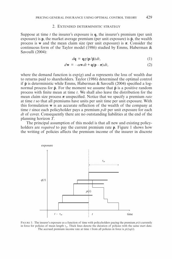
FIGURE 1: The insurer’s exposure as a function of time with policyholders paying the premium p (t) currentlyin force for policies of mean length tm. Thick lines denote the duration of policies with the same start date.

The accrued premium income rate at time t from all policies in force is p(t)q(t).

2. EXTENDED DETERMINISTIC STRATEGY

Suppose at time t the insurer’s exposure is q, the insurer’s premium (per unitexposure) is p, the market average premium (per unit exposure) is p, the wealthprocess is w and the mean claim size (per unit exposure) is p. Consider thecontinuous form of the Taylor model (1986) studied by Emms, Haberman &Savoulli (2004):

dq = qg (p /p)dt, (1)

dw = –awdt + q(p – p)dt, (2)

where the demand function is exp(g) and a represents the loss of wealth dueto returns paid to shareholders. Taylor (1986) determined the optimal controlif p is deterministic while Emms, Haberman & Savoulli (2004) specified a log-normal process for p. For the moment we assume that p is a positive randomprocess with finite mean at time t. We shall also leave the distribution for themean claim size process p unspecified. Notice that we specify a premium rateat time t so that all premiums have units per unit time per unit exposure. Withthis formulation w is an accurate reflection of the wealth of the company attime t since each policyholder pays a premium pdt per unit exposure for eachdt of cover. Consequently there are no outstanding liabilities at the end of theplanning horizon T.

The principal assumption of this model is that all new and existing policy-holders are required to pay the current premium rate p. Figure 1 shows howthe writing of policies affects the premium income of the insurer in discrete

PRICING GENERAL INSURANCE USING OPTIMAL CONTROL THEORY 429

terms. The change in wealth at time t due to premium income is denoted bythe term pqdt in the wealth equation. Such an assumption is attractive sinceit means that all the random processes are Markov. It is reasonable if the pre-mium rate does not change substantially over the course of a policy.

The demand parameterisation g(p /p) in Taylor (1986) took two forms:

g = a (1 – p /p), (3)

g = –a log(p /p), (4)

corresponding to an exponential or constant elasticity demand function. Herea is a constant which determines how much exposure is generated by a changein relative premium. The first of these forms was discussed solely in Taylor(1986), whilst the second has found widespread use in the financial literature(Lilien & Kotler 1983). Emms, Haberman & Savoulli (2004) considered two pre-mium strategies and maximised the expected total utility of wealth. A similaranalysis can be performed by specifying the simpler objective function

V = maxp

{� [w(T) | S(0)]},

that is maximising the expected wealth at the end of the planning horizon T giveninformation on the state S at time t = 0. The adoption of a fixed form for thestrategy effectively places a constraint on the variation of the premium.

We can generalise one of the premium strategies adopted in Emms, Haber-man & Savoulli (2004) by considering the premium strategy

p = k(t)p. (5)

Emms, Haberman & Savoulli fixed k as a constant while here we maximise theobjective over the functional k(t). The deterministic function k(t) need not besmooth and so it is useful for the analysis of models such as (1)-(2). Given theoptimal relative premium k(t), the corresponding optimal premium is sto-chastic and for the premium to be non-negative we require k ≥ 0.

The demand functions and the form of strategy ensure that the exposureq(t) is deterministic. This considerably simplifies the model and is one reasonfor adopting a strategy such as (5). If we adopt the terminology of optimal con-trol theory then the control variable is k and the state variable is the exposureq which is governed by

q = qg(k).

For both the constant elasticity and exponential demand functions g is adecreasing function of k. Note the forthcoming arguments still apply if wesplit up the exposure equation into new business generation and negative drift(representing policy termination) as long as the parameterisation of new busi-ness is of a similar form to the demand functions (3) and (4).

Taking the expectation of the wealth equation given information up untilt = 0 we obtain


� [w(T)] = e–aT w F dt0T

0+ #] g; E,

where

F = F (q,k,t) = eatq(kmp – mp). (6)

Here we adopt the notation

mX(t; s) = � [X(t) |S(0) = s], (7)

where S is the state of the system. Consequently the problem can be writtenin one of the standard forms for control theory (Sethi & Thompson 2000).We wish to determine the value function

, , ,maxV J F q k t dtk

T

0 0= =

$# ^ h' 1 (8)

where the optimal control k* is denoted with an asterisk. The value of this objec-tive function determines the maximum value of the expected terminal wealth.

The necessary conditions for an optimal control are determined by the Maxi-mum Principle which can be stated in terms of the Hamiltonian defined by

H(q,k,l, t) = F (q,k, t) + lqg (k), (9)

where l is a Lagrange multiplier. The Maximum Principle states that

H (q*,k*,l, t) ≥ H (q*,k,l, t),

for all k ≥ 0. For the exponential demand function g = a (1 – k) and thereforethe Hamiltonian is linear in the control. The optimal control is bang-bang:for l ≤ 0, k* = 3 while for l > 0, k* = 0 or 3 depending on the parameters ofthe model. If l > 0, k* = 0 then this is the ultimate loss-leader: an insurer givesaway insurance in order to capture the whole market and then charges thosecustomers an infinite premium at t = T in order to generate infinite wealth.If k* = 3 for t ! [0,T ] then it is optimal not to sell insurance.

For the constant elasticity demand function g = –a logk and the Hamilto-nian is

H(q,k,l, t) = eatq (kmp – mp) – laq log k. (10)

If we suppose that the maximum of H over k ! (0,3) is given by Hk = 0 thenusing (10) yields

eatmp – la /k = 0. (11)

Since k must be positive this requires l to be positive also. This equation whencoupled to the adjoint equation


l = – Hq = – eat(kmp – mp) + la log k (12)

determines an optimal control and ultimately leads to the Euler-Lagrangeequation of the Calculus of Variations (Gelfand & Fomin 2000). However, fora maximum of H the second-order condition is Hkk ≤ 0 at k = k*. From (10)we find

Hkk = kaql

2> 0.

for k > 0, so that the turning point is a minimum. Looking at the form of theHamiltonian it is clear that the optimal control is degenerate and not unique:if l ≤ 0 then k* = 3, while if l > 0 then k* = 0 or 3.

We have shown that for both demand functions (3) and (4) the optimalcontrol is degenerate. Although for some demand functions it is simple to writedown an equation that an extremal must satisfy, it is important to ensure thatwe actually have a maximal extremal. This applies to both deterministic andstochastic dynamic strategies, the latter of which are determined by a Bellmanequation. Since the deterministic strategy generates infinite terminal wealththe solution to the Bellman equation for the (unconstrained) problem is alsobang-bang.

A bang-bang strategy is optimal because of the principal assumption of thecontinuous model (1)-(2), that is, an insurer requires all existing customers topay the current premium rate. However, there is a restriction on just how bigan increase existing policyholders will be prepared to pay for insurance beforeterminating their cover. The optimal strategy is dependent on the value of thisincrease. One solution to the problem is to place a constraint on the premiumstrategy so that premium rates cannot change substantially over the policy (seeEmms, Haberman & Savoulli 2004). An alternative approach is to change theassumptions of the model and this is the approach we adopt next.

3. ACCUMULATED PREMIUM INCOME

We describe a simplified continuous version of the model proposed by Gerrard &Glass (2004). We split up the change in exposure into that lost due to policytermination and that gained due to new business (or renewals). To do this weneed a parameterisation for the rate of generation of new business n. Motivatedby the previous demand functions (3) and (4) we adopt a relationship of theform

n = qG (p /p), (13)

where G is a non-negative demand function. This parameterisation reflects theidea that the reputation of a company is proportional to its exposure in themarket and that it is in part the reputation of an insurer which increases itslikelihood to generate new business. New business generation is also deter-mined by the premium that the insurer sets relative to the market, which is


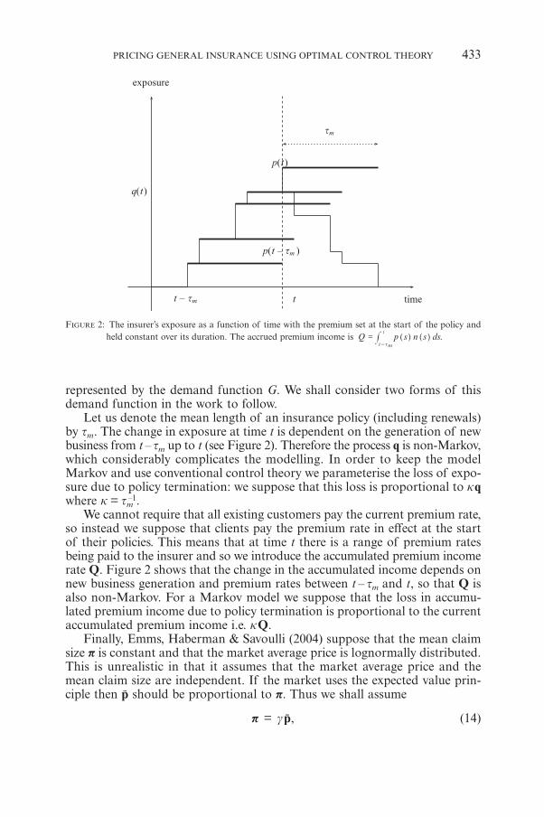
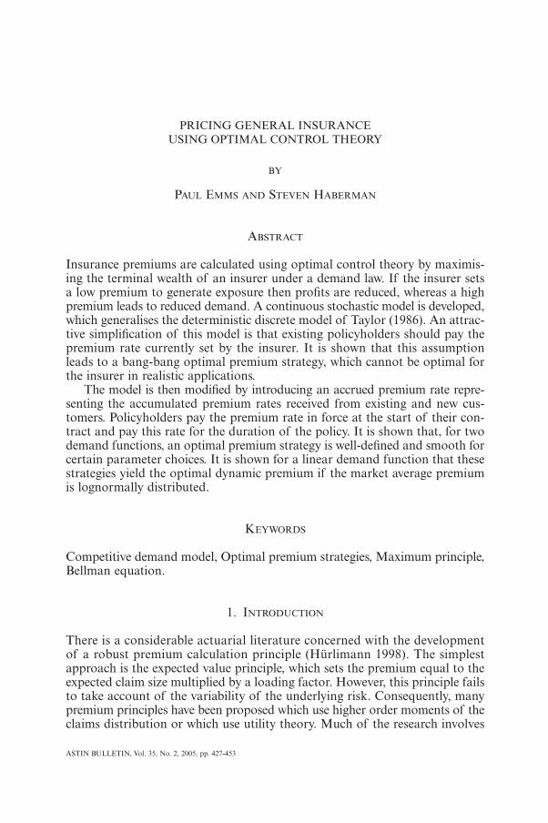
FIGURE 2: The insurer’s exposure as a function of time with the premium set at the start of the policy andheld constant over its duration. The accrued premium income is .Q p s n s ds

t

t t=

- m# ] ]g g

represented by the demand function G. We shall consider two forms of thisdemand function in the work to follow.

Let us denote the mean length of an insurance policy (including renewals)by tm. The change in exposure at time t is dependent on the generation of newbusiness from t – tm up to t (see Figure 2). Therefore the process q is non-Markov,which considerably complicates the modelling. In order to keep the modelMarkov and use conventional control theory we parameterise the loss of expo-sure due to policy termination: we suppose that this loss is proportional to kqwhere k = tm

–1.We cannot require that all existing customers pay the current premium rate,

so instead we suppose that clients pay the premium rate in effect at the startof their policies. This means that at time t there is a range of premium ratesbeing paid to the insurer and so we introduce the accumulated premium incomerate Q. Figure 2 shows that the change in the accumulated income depends onnew business generation and premium rates between t – tm and t, so that Q isalso non-Markov. For a Markov model we suppose that the loss in accumu-lated premium income due to policy termination is proportional to the currentaccumulated premium income i.e. kQ.

Finally, Emms, Haberman & Savoulli (2004) suppose that the mean claimsize p is constant and that the market average price is lognormally distributed.This is unrealistic in that it assumes that the market average price and themean claim size are independent. If the market uses the expected value prin-ciple then p should be proportional to p. Thus we shall assume

p = gp, (14)


where the constant g is a measure of the market loading factor. It is expectedthat g K 1 so that the market, on average, makes money selling insurance. Wemay consider the case that g is a deterministic or stochastic function of timein subsequent work.

With these assumptions the modified model is

dq = (n – kq)dt, (15)

dQ = (pn – kQ)dt, (16)

dw = –awdt + Qdt – gpqdt. (17)

Again, we adopt the deterministic strategy (5) so that the exposure q and therate of generation of new business n are deterministic. We assume that thereis an explicit expression for mp independent of the other state variables so thatthere are now two unknown state variables: q and mQ. For example, if p is log-normally distributed with drift m then mp = p(0)emt using the notation definedin (7).

The first state equation is (15) whilst the second comes from taking the expec-tation of (16), which yields

dtdmQ = qkG (k)mp – kmQ,

using (5) and (13). On integrating this equation we obtain

,

m t m e m s n s ds

m e m s b db

0

0

Q Qs tt

p

Qs b tB t

p

k

k

0

0

= +

= +

-

-

#

#

] ]]

] ]

]]]

]

]^

g gg

g g

gg g

g

gh

(18)

where B(t) = n st

0# ] gds is the total amount of business generated over time t.

Here we have supposed that B is a strictly increasing function of t so that itsinverse t = t (B) is well-defined.

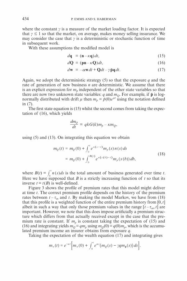
Figure 3 shows the profile of premium rates that this model might deliverat time t. The correct premium profile depends on the history of the premiumrates between t – tm and t. By making the model Markov, we have from (18)that this profile is a weighted function of the entire premium history from [0, t]albeit in such a way that only those premium values in the range [t – tm, t] areimportant. However, we note that this does impose artificially a premium struc-ture which differs from that actually received except in the case that the pre-mium rate is constant. If mp is constant taking the expectation of (15) and(16) and integrating yields mQ = qmp using mQ(0) = q(0)mp, which is the accumu-lated premium income an insurer obtains from exposure q.

Taking the expectation of the wealth equation (17) and integrating gives

a a q .m t e m e m s m s dsg0t st

0= + --

w Qw p#] ] ] ]^g g g gh; E


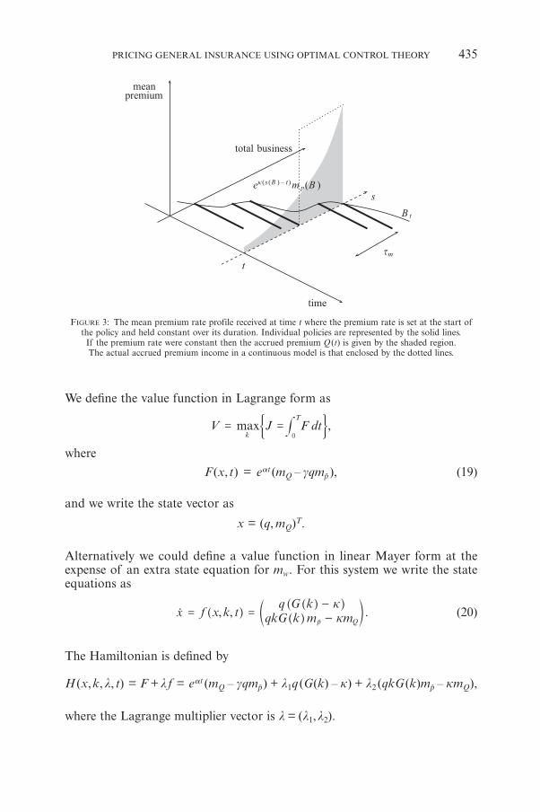
FIGURE 3: The mean premium rate profile received at time t where the premium rate is set at the start ofthe policy and held constant over its duration. Individual policies are represented by the solid lines.

If the premium rate were constant then the accrued premium Q (t) is given by the shaded region.The actual accrued premium income in a continuous model is that enclosed by the dotted lines.

We define the value function in Lagrange form as

,maxV J F dtk

T

0= = #' 1

where

F (x, t) = eat (mQ – gqmp), (19)

and we write the state vector as

x = (q, mQ)T.

Alternatively we could define a value function in linear Mayer form at theexpense of an extra state equation for mw. For this system we write the stateequations as

, , .f x k tq G k

qkG k m mkkx

Qp= =

--]

]^

]dg

g h

gn (20)

The Hamiltonian is defined by

H (x,k,l, t) = F +l f = eat (mQ – gqmp) + l1q (G(k) – k) + l2 (qkG (k)mp – kmQ),

where the Lagrange multiplier vector is l = (l1,l2).


We suppose the optimal control k* is given by the first order condition fora maximum of H, the state equations and the adjoint equations:

Hk = 0, (21)x = Hl, (22)l = –Hx. (23)

We must also ensure the second order condition holds: Hkk ≤ 0 at k = k*. Thelast two equations are the canonical Euler equations (Gelfand & Fomin 2000)and reduce to the Euler-Lagrange equation if the control is sufficiently smooth.The boundary conditions for this system are

x(0) = (q(0), mQ(0))T, l (T ) = 0,

the last of which is the transversality condition. In general, for two state vari-ables, this is a fourth-order boundary value problem. However, H is linear inthe state variables and Hk = 0 only depends on mp so that the system decouplesindependently of the particular parameterisation for G. In order to determinethe optimal control k* we need only solve the initial value problem consistingof the adjoint equations (23) and the transversality condition.

The second of the adjoint equations is independent of the choice of demandfunction G. From (19) and (20) we have

l2 = – HmQ= kl2 – eat, (24)

with boundary condition l2(T) = 0. This can be integrated immediately toobtain

l2(t) =a

ek

a

-

t

(1 – e(k – a) (t –T )). (25)

Consequently for 0 ≤ t ≤ T we have l2 ≥ 0.

3.1. Power law demand function

The demand function G must be a non-negative decreasing function of therelative premium price. Therefore a suitable parameterisation, which is definedfor all positive premiums, takes the form of a power law:

G = b1k– a1, (26)

where a1, b1 > 0: a1 is dimensionless while b1 has units per unit time. AlthoughG is defined for all k > 0, (26) is an unrealistic parameterisation as k becomeslarge. If the optimal strategy depends upon new business generation for largerelative premium rates then this is not a good model for the demand func-tion.


The Hamiltonian for this demand function is

H = eat (mQ – gqmp) + l1q (b1k– a1 – k) + l2(qb1k– a1+1mp – kmQ),

which has derivatives

Hk = qb1k– a1 –1 ((1 – a1)l2mpk – a1l1),

Hkk = a1b1qk– a1 –2 ((a1 + 1)l1 – (1 – a1)l2kmp).

Suppose the extremum of H is at an interior point ki*, that is ki* ! (0,3). There-fore the optimal strategy is given by Hk = 0:

ki* = ,aa

m ll

1 p1

1

- 2

1d n (27)

which yields a maximum providing that

Hkk = a1b1qki*– a1 –2l1 < 0.

Consequently there is an interior maximum of H if l1 < 0 and ki* ! 0. Furtherfrom (25) and (27) we must have a1 > 1. If there is no interior maximum theoptimal strategy is at either end-point of k. The optimal behaviour can besummarised by the following table for a1 > 1:

l2 = 0 l2 > 0

l1 < 0 k* = 3 interiorl1 = 0 undefined k* = 0l1 > 0 k* = 0 k* = 0

The remaining Lagrange multiplier is determined by

l1 = gmpeat + l1k + l1b1 ,a aa m

ll

11 1 a

p

1 1

2

-

-

1

11

b]dl

gn (28)

using (25) with boundary condition l1(T ) = 0. This is similar to a Bernoulliequation but it is non-homogeneous and so in general it does not have an ana-lytical solution.

We nondimensionalise the market average premium using its initial value.The remaining scales are taken as

b1l2 = w, b1l1 = p(0)l, t = T (1 – s), a = aT,

k = Kb1, e = (b1T )–1, mp = p(0)M(s).

Substituting these scales into (28) we obtain the non-dimensional adjoint equation:


dsde l = –gM(s)ea(1– s) – Kl – ,a a

a M sl

w1

1 1 a

--

1 1

11

b] ]dl

g gn (29)

where from (25)

,a

sKe ew 1

aa

ss

1 Ke=

--

--

e]

]]`g

gg j

and the optimal strategy is

ki* = .a Mwl

11- 1

b l (30)

At s = 0, l = w = 0 so that ki* is undefined. We can only find the limiting behav-iour numerically since substituting Taylor series expansions for l and w abouts = 0 leads to the algebraic equation:

el�(0) = –gM (0)ea – ea aa M e

l11

01 0

�

a a

1

1

--

1

1

b]

] ]fl

g

g gp .

Given the numerical root of this equation we can integrate (29) numerically withinitial value l(ds) = l�(0)ds.

If we suppose e % 1 then to leading-order we have w ~ ea (1 – s)K and an alge-braic equation for l:

gM(s)ea (1 – s) – K (–l) + .a aa

KM s e

l11 1

0a s a

1

1

--

-=

-

1

1

1

b c]

]]

fl mg

gg

p (31)

In general the solution to this equation can only be determined numerically.For simplicity, we suppose p is constant so that M / 1. In order to gener-

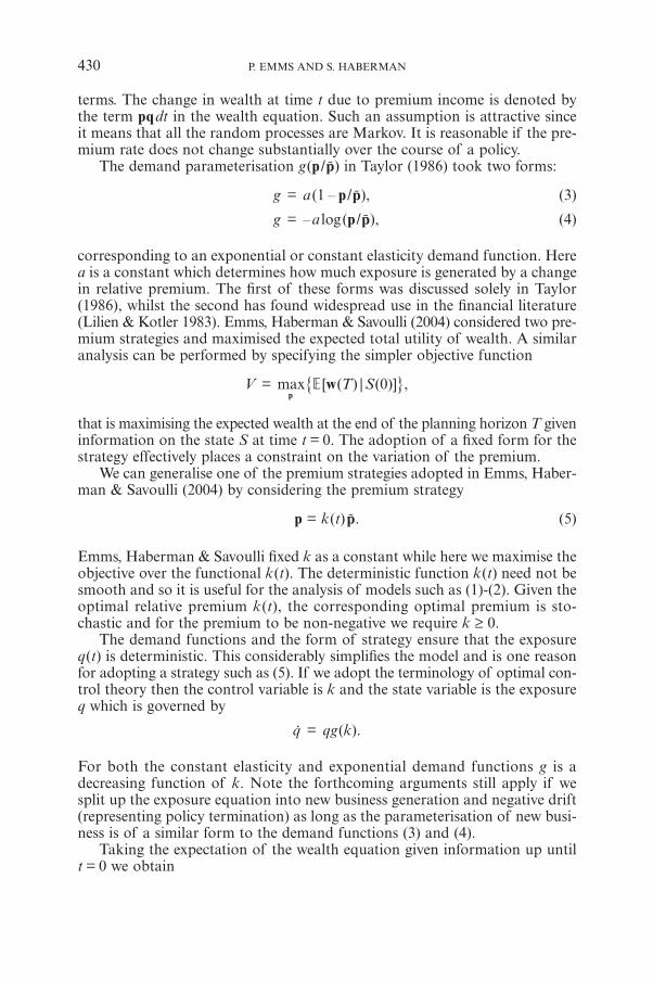
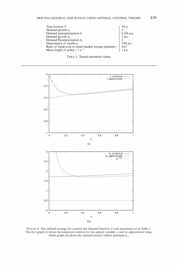
ate a parameter set we shall suppose that if the insurer sets its premium at 80%of the market value then this leads to a 40% increase in the insurer’s exposureafter one year. Thus we choose a1 = 2 and obtain b1 = 0.256 p.a. from (26). Themean policy length is set at one year and the planning horizon is 10 years.Depreciation of wealth is taken as 6% and the premium ratio g = 0.67. Figure 4shows the numerical solution to (29) and (31) for comparison using the sam-ple data in Table 1. The strategy proceeds from s = 1 corresponding to t = 0 tos = 0 at time t = T. Notice that there is a region of thickness e where the alge-braic equation does not give a good approximation to the adjoint differentialequation. From (15) the state equation for the exposure is

dq = qb1(k –a1 – K )dt. (32)

It can be seen in Figure 4 (ii) that the optimal strategy ki* is always aboveK –1/a1 so that exposure is decreasing exponentially with increasing time t. Thusfor this parameter set the optimal strategy represents a withdrawal from themarket.


(i)

(ii)

FIGURE 4: The optimal strategy for a power law demand function G with parameters as in Table 1.The first graph (i) shows the numerical solution for the adjoint variable l1 and its approximate value,

whilst graph (ii) shows the optimal interior relative premium ki*.


Time horizon T 10 yrDemand growth a1 2Demand parameterisation b1 0.256 p.a.Demand growth a2 2 p.a.Demand Parameterisation b2 1Depreciation of wealth a 0.06 p.a.Ratio of break-even to initial market average premium g 0.67Mean length of policy t = k –1 1 p.a.

TABLE 1: Typical parameter values.

(i)

(ii)

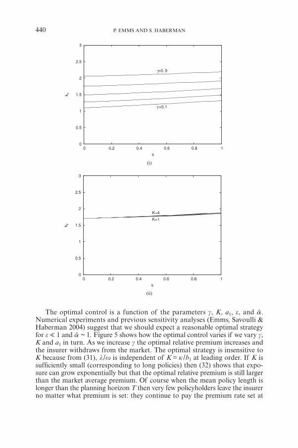
The optimal control is a function of the parameters g, K, a1, e, and a.Numerical experiments and previous sensitivity analyses (Emms, Savoulli &Haberman 2004) suggest that we should expect a reasonable optimal strategyfor e % 1 and a ~ 1. Figure 5 shows how the optimal control varies if we vary g,K and a1 in turn. As we increase g the optimal relative premium increases andthe insurer withdraws from the market. The optimal strategy is insensitive toK because from (31), l /w is independent of K = k /b1 at leading order. If K issufficiently small (corresponding to long policies) then (32) shows that expo-sure can grow exponentially but that the optimal relative premium is still largerthan the market average premium. Of course when the mean policy length islonger than the planning horizon T then very few policyholders leave the insurerno matter what premium is set: they continue to pay the premium rate set at


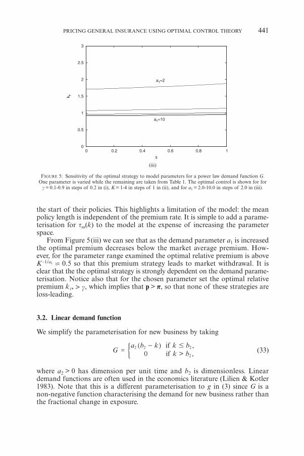
FIGURE 5: Sensitivity of the optimal strategy to model parameters for a power law demand function G.One parameter is varied while the remaining are taken from Table 1. The optimal control is shown for for

g = 0.1-0.9 in steps of 0.2 in (i), K = 1-4 in steps of 1 in (ii), and for a1 = 2.0-10.0 in steps of 2.0 in (iii).

(iii)

the start of their policies. This highlights a limitation of the model: the meanpolicy length is independent of the premium rate. It is simple to add a parame-terisation for tm(k) to the model at the expense of increasing the parameterspace.

From Figure 5(iii) we can see that as the demand parameter a1 is increasedthe optimal premium decreases below the market average premium. How-ever, for the parameter range examined the optimal relative premium is aboveK –1/a1 c 0.5 so that this premium strategy leads to market withdrawal. It isclear that the the optimal strategy is strongly dependent on the demand parame-terisation. Notice also that for the chosen parameter set the optimal relativepremium ki* > g, which implies that p > p, so that none of these strategies areloss-leading.

3.2. Linear demand function

We simplify the parameterisation for new business by taking

,> ,G

a b k k bk b

ifif0

2 2 2

2

#=

-] g( (33)

where a2 > 0 has dimension per unit time and b2 is dimensionless. Lineardemand functions are often used in the economics literature (Lilien & Kotler1983). Note that this is a different parameterisation to g in (3) since G is anon-negative function characterising the demand for new business rather thanthe fractional change in exposure.


The Hamiltonian in this case is

H = eat(mQ – gqmp) + l1q(a2(b2 – k) – k) + l2(qka2(b2 – k) mp – kmQ),

which has derivatives

Hk = –a2ql1 + l2qmp a2(b2 – 2k),

Hkk = –2l2qmp a2,

if k ≤ b2. Therefore we have a maximum for H at

ki* = ,b m ll

21

p2

2

1-d n (34)

which gives the optimal interior strategy providing that 0 ≤ ki* ≤ b2 and l2 > 0.The remaining adjoint equation determines the optimal interior control:

l1 = gmpeat – l1(a2(b2 – ki*) – k) – l2a2ki*(b2 – ki*) mp, (35)

with boundary condition l1(T ) = 0. The second Lagrange multiplier is just afunction of t so we can substitute (34) into (35) to obtain

l1 = gmpeat – ,a b m a b

mal

l k ll

4 2 4p

p

2 2

22 2 2

2

22

- - -11

c m (36)

which is a Riccati equation.Next we rescale using the following change of variables:

t = T (1 – s), a2l1 = p(0)l, a2l2 = w, mp = p(0)M(s) (37)

and introduce the following nondimensional parameters:

k = Ka2, e = a T12

, a = aT.

Note that the definition of K and e has changed from the previous section becauseof the change in demand function. From (15) the exposure is governed by

,> .dq

qa b k Kqa K

k bk b

ifif

2 2

2

2

2

#=

- --] g

( (38)

If K ≥ b2 then policies expire at a rate greater than the rate at which new busi-ness is generated irrespective of the level of the relative premium. This is clearlyunrealistic so we must have K < b2.

The nondimensional Riccati equation is


,dsd b M s s b K M s s M s ee l w

l wl g

4 2 4a s2

2

22

1= + - + - -] ]c

] ]]

]g gm

g gg

g (39)

with

,a

sKe ew 1

aa

ss

1 Ke=

--

--

e]

]]`g

gg j (40)

and the boundary condition is l(0) = 0. In terms of these new variables the opti-mal interior strategy is

ki* = ,b Mwl

21

2 -b l (41)

providing that |l | < Mw. Since both l = w = 0 at s = 0, this expression is undefinedat end of the time horizon. However, if we suppose that l is sufficiently smoothnear s = 0 then a Taylor series expansion substituted into (39) gives

ki* =21 (b2 + g), as s " 0+. (42)

This expression gives the terminal optimal relative premium rate.Let us suppose e % 1. To leading-order w ~ e a (1 – s) /K and

,MKe

K b K b K Kl

g2 2/

a s 1

22

2

1 2

+- - - +

-

J

L

KKK ]

`N

P

OOOg

j(43)

providing that

g ≥ gc = b2 – K. (44)

Again, we suppose that if the insurer sets its premium at 80% of the marketpremium then that leads to a gain in exposure of 40% over one year. Thus wechoose a2 = 2 p.a. and obtain b2 = 1 from (33). The other parameters are takenfrom Table 1 and yield gc = 1/2. If g < 1/2 then the optimal control does not equi-libriate. In this case there is the possibility that the optimal control becomesnegative or even that there is a spontaneous singularity for s ! (0,1]. Using (43)the approximate optimal interior strategy is

ki* = b2 – K – (K2 – b2K + Kg)1/2. (45)

The leading-order value of ki* is independent of both M and s. It should beremembered that these approximate expressions only remain valid if the solutionto the Riccati equation does equilibriate. In the following numerical calculationswe find that as the solution tends towards a bang-bang control then these approx-imations become invalid.


(ii)

(i)

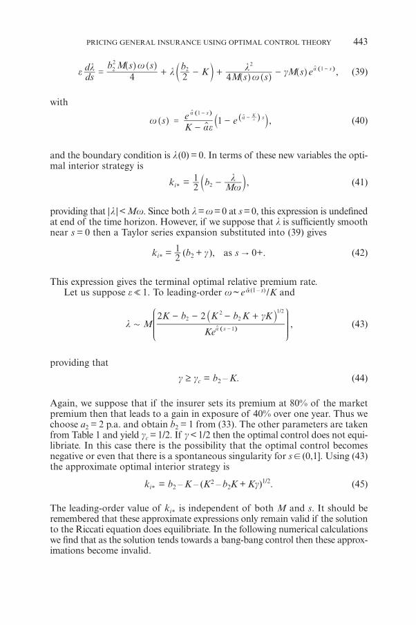
Figure 6 shows the approximate premium strategy along with the numeri-cal solution of the Riccati equation (39) using the parameters in Table 1. Forthe moment we set b2 = 1 so that there is no demand for insurance if theinsurer’s premium is above market average. We shall relax this assumption inthe forthcoming sensitivity analysis. In addition, we set M / 1 so that there isno drift in the market average premium. Figure 6 (i) reveals that there is an innerregion where the approximate expression for l does not satisfy the boundarycondition however, this region appears unimportant, when we plot the approxi-mate optimal premium ratio ki*. Note that the strategy proceeds over timefrom s = 1 to s = 0 and, the exposure is always decreasing as s decreases (sincek > b2 – K) so that this strategy effectively represents a gradual withdrawal fromthe market. In contrast to the power law demand function, the optimal controlki* for a linear demand function increases over time.

The optimal control is a function of six parameters: g, K, b2, M, a and e.The last of these parameters, e, is a measure of how fast the adjoint l1 reachesits equilibrium (should it do so). Figure 7(i)-(iv) show how the optimal controlvaries as we vary each of these parameters in isolation.


FIGURE 6: The optimal premium strategy for a linear demand function G with parameters taken fromTable 1. Graph (i) shows the adjoint variable l while (ii) shows the optimal relative premium ki*.

(i)

(iii)

(ii)


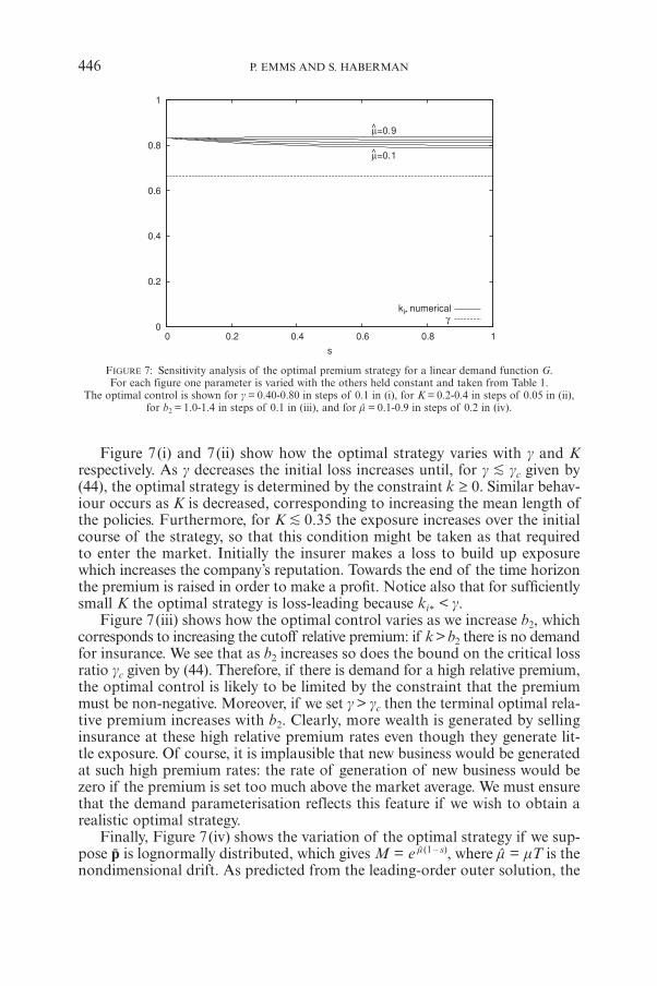
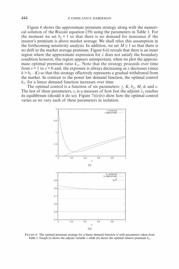
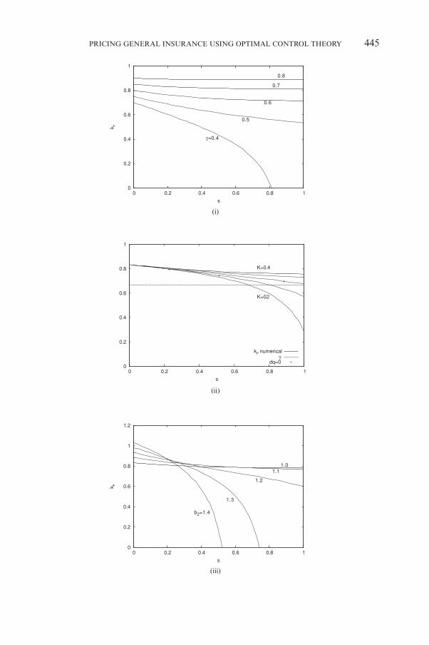
FIGURE 7: Sensitivity analysis of the optimal premium strategy for a linear demand function G.For each figure one parameter is varied with the others held constant and taken from Table 1.

The optimal control is shown for g = 0.40-0.80 in steps of 0.1 in (i), for K = 0.2-0.4 in steps of 0.05 in (ii),for b2 = 1.0-1.4 in steps of 0.1 in (iii), and for m = 0.1-0.9 in steps of 0.2 in (iv).

Figure 7(i) and 7(ii) show how the optimal strategy varies with g and Krespectively. As g decreases the initial loss increases until, for g K gc given by(44), the optimal strategy is determined by the constraint k ≥ 0. Similar behav-iour occurs as K is decreased, corresponding to increasing the mean length ofthe policies. Furthermore, for K K 0.35 the exposure increases over the initialcourse of the strategy, so that this condition might be taken as that requiredto enter the market. Initially the insurer makes a loss to build up exposurewhich increases the company’s reputation. Towards the end of the time horizonthe premium is raised in order to make a profit. Notice also that for sufficientlysmall K the optimal strategy is loss-leading because ki* < g.

Figure 7(iii) shows how the optimal control varies as we increase b2, whichcorresponds to increasing the cutoff relative premium: if k > b2 there is no demandfor insurance. We see that as b2 increases so does the bound on the critical lossratio gc given by (44). Therefore, if there is demand for a high relative premium,the optimal control is likely to be limited by the constraint that the premiummust be non-negative. Moreover, if we set g > gc then the terminal optimal rela-tive premium increases with b2. Clearly, more wealth is generated by sellinginsurance at these high relative premium rates even though they generate lit-tle exposure. Of course, it is implausible that new business would be generatedat such high premium rates: the rate of generation of new business would bezero if the premium is set too much above the market average. We must ensurethat the demand parameterisation reflects this feature if we wish to obtain arealistic optimal strategy.

Finally, Figure 7(iv) shows the variation of the optimal strategy if we sup-pose p is lognormally distributed, which gives M = e m(1 – s), where m = mT is thenondimensional drift. As predicted from the leading-order outer solution, the


variation of this parameter has little effect on the optimal strategy. The meanof the market average premium M(0) cancels in the inner region so that thereis little variation in the optimal control over the entire time horizon. The optimalcontrol shows little variation with a so the results are not shown.

4. PURE STOCHASTIC STRATEGY

We have found smooth deterministic optimal strategies for an accrued pre-mium model for certain parameter choices. Using the linear demand functionwe look next for the dynamic optimal premium and derive the correspondencebetween this premium and the deterministic premium strategy.

Let us suppose the process for the market average premium follows an Itoprocess

dp = mtdt + stdZt, (46)

where Zt is a standard Brownian motion and the drift mt and the volatility stdepend on time and the current state but not the insurer’s premium. We usethe relative premium k = p/p as the control and define the value function to maxi-mise the expected terminal wealth:

V(p,q,Q,w, t) =max

k{� [w(T ) | p(t) = p,q(t) = q,Q(t) = Q,w(t) = w]}.

(47)

Bellman’s principle of optimality states that

V(p,q,Q,w, t) =max

k{� [V (p + dp,q + dq,Q + dQ,w + dw, t + dt) | (48)

p(t) = p,q(t) = q,Q(t) = Q,w(t) = w]}.

Therefore rearranging on the right-hand side we obtain the Bellman equation

.max� dtdV

0k

t =: D

For the insurance model (46) and (15)-(17) the Bellman equation is

Vt + mVp +21 s2Vpp + Vw(–aw + Q – gpq ) +

maxk

{q (G – k)Vq + (pqG – kQ)VQ} = 0, (49)

with boundary condition

V (t = T ) = w, (50)

providing the value function is sufficiently smooth.


The first order condition for a maximum gives

G�Vq + VQ p (G + kG�) = 0.

For the demand function (33), G� = –a2 providing k ≤ b2 so that this conditionbecomes

Q

q ,k b VVp2

12= -d n (51)

which is similar in form to (34). If the value function is sufficiently smooth andwe write the “shadow prices’’ Vq = l1 and VQ = l2 then the optimal premiumshave the same form (see p. 229, Yong & Zhu 1999). This demonstrates the widercorrespondence between the Maximum Principle and Dynamic Programming.Substituting (51) into the Bellman equation removes the maximum operator:

Vt + mVp +21 s2Vpp + Vw(–aw + Q – gpq ) +

Q

q

Q

qq Q .q a b V

VV

a qb

V

VQ Vk kp

pp2 4

02 2

2

2 2

2

+ - + - - =2 2

J

L

KK

J

L

KKde

N

P

OO

N

P

OOn o (52)

This is a quasi-linear partial differential equation with four space variables.Given its high dimension and nonlinearity this problem appears difficult tosolve numerically. However, by assuming a particular form for the value functionmotivated by the deterministic optimisation problem, we can find a solutionof (52) and apply a verification theorem (Fleming & Rishel 1975).

On the boundary t = T, V = w and therefore Vq = VQ = 0 so that the pre-mium given by (51) is undefined in the same way as it was for the deterministicstrategy. If we approximate Vt by a first-order difference then

t ,V tV T V T t

dd

.- -] ]g g

where dt is a small time step. Substituting into the Bellman equation (52) yields

V(T – dt) = w + (–aw + Q – gpq)dt, (53)

so that VQ = dt and Vq = –gpdt at t = T – dt providing the spatial boundary con-ditions are consistent with the finite difference approximation (53). Conse-quently the terminal premium is well-defined as t " T – and is given by

pT – =21 p (b2 + g). (54)

This should be compared with the optimal deterministic strategy given by (42):near the boundary the terminal premium is identical to the deterministic optimal


premium strategy as long as the control is sufficiently smooth. The result holdsirrespective of the distribution of p.

Given the structure of (53) we further restrict the process for p by suppos-ing m = m(p,t) and s2 = s2(p,t). Now we look for a value function of the form

V = e–aT(eatw + L1(p, t)q + L2(t)Q ), (55)

with L1(T) = L2(T) = 0. Consequently, from (51) a candidate for the dynamicoptimal control is

kc( p, t) =,

,b tt

LLp

p21

2

1-2

]

^d

g

hn (56)

as long as the control is interior. Substituting (55) into (52) yields a PDE forL1 and an ODE for L2:

L1t + m(p,t)L1p +21 s2(p,t)L1pp + a b k

21

2 2 -b lL1+41 a2 pb2

2L2 +a

LL

p4 2

2 1

2

= geatp. (57)

L2 = kL2 – eat. (58)

The equation for L1 is a semi-linear PDE and, in general, can only be solvednumerically. The equation for L2 is identical to (24) so that its solution is givenby (25).

We can make further progress by supposing p is lognormally distributedso that its drift and volatility are linear in the state variable: m(p,t) = mp ands2(p,t) = s2p. Consequently L1 takes the form

L1(p,t) = mp pl1(t), (59)

where l1 satisfies

l1 = gmpeat –41 a2 b2

2L2mp – l1 .a b ma

klL42

1

p2 2

2

22

- - 1b l (60)

Now the candidate dynamic premium strategy is of the form pc = k(t)p from(56) and (60) is identical to (36).

The deterministic strategy (5) is of a similar form to the candidate dynamicpremium in the case that the market average premium is lognormally distri-buted and the control is smooth. In (7) we take the expectation of the governingprocesses based on information up until t = 0. However, we could instead takeconditional expectations using the information available up until time t. Theanalysis in Section 3.2 would be identical and the optimal premium strategywould be the same except that the state equations must be integrated usingthe current state rather than that at time t = 0. Consequently, if we evaluate thedeterministic premium strategy then this yields the candidate optimal dynamic


premium in the form pc = ki*p if we use the current value of the lognormally dis-tributed market average premium. However, if p has some other distribution thenwe must solve the PDE (57) numerically with boundary condition L1(p,T) = 0.

It remains to ascertain under what conditions the candidate premium strat-egy (56) is optimal. If the market average premium is lognormally distributedthen we can apply the verification Theorem 4.1 of Fleming & Rishel (1975) p. 159.Let us restrict the set of feedback controls to

U = {k(t) !C1(t) : 0 ≤ k(t) ≤ b2, 0 ≤ t ≤ T}

so that the exposure equation (15) has smooth bounded coefficients. We assumethat there exists a sufficiently smooth unique solution to (60) over [0,T ] whichleads to a control k(t)! U. The value function defined by (55) and (59) is twicecontinuously differentiable in the state variables because it is linear in those vari-ables and L2(t) is a smooth function of time. The value function is also oncecontinuously differentiable in time so V ! Cp

2,1(Q) where the domain Q = �4 ≈(0,T ) using the notation of Fleming & Rishel.

By construction V satisfies the Bellman equation (49) and boundary con-dition (50) providing the first order condition yields the maximum in the equation.The expression inside the maximum operator is a quadratic function of k wherethe coefficient of k2 is

– eaTa2 pqL2(t) ≤ 0

so that the maximum is given by the first order condition as long as kc! U.It remains to determine whether the feedback control kc = kc(t) leads to a well-defined state trajectory, that is, we must verify that the control is admissible.If we substitute the control into the state equations (15)-(17) then we obtaina system of linear stochastic differential equations:

dp = mpdt + spdZt,

dQ = (k(t)q(t)G (k(t))p – kQ)dt,

dw = –awdt + Qdt – gq(t)pdt.

The exposure, q (t), is deterministic and governed by a linear equation withbounded smooth coefficients so that it is integrable over [0,T]. Therefore, by theuniqueness and existence Theorem 4.1 of Fleming & Rishel (1975) p. 118 thereis a unique state trajectory corresponding to the optimal control. The linearityand the smoothness of the coefficients ensure that both the Lipschitz and lineargrowth conditions are satisfied over the domain Q. Consequently the conditionsof Theorem 4.1 of Fleming & Rishel (1975) are satisfied and kc(t) ! U is theoptimal control.

The verification of optimality reduces to the existence of a smooth solu-tion of the Riccati equation (60) which yields a control in the set U. It is wellknown that Ricatti equations may blow-up in finite time (see Bender & Orszag1978). We can see this behaviour in Figure 7(i)-(iii) as g, K are decreased orb is increased. The validity of the optimal control depends implicitly on the


parameters through the solution of (60): if for a given parameter set the com-puted control lies in U then it is the optimal control. This is the case for anumber of the controls in Figure 7. In the absence of an analytical solution,the range of parameters which lead to either negative controls or blow-up mustbe determined numerically.

5. CONCLUSIONS

Emms, Haberman & Savoulli (2004) found the optimal insurance premium giventhat the relative insurer to market average premium was constant: p /p = k.They found that the insurer should set k so that p is just above the breakevenrate if there is no drift in the market average premium. We have modified theirmodel in a number of ways.

First, we suppose that the loss ratio g = p /p is constant. Emms, Haberman &Savoulli (2004) supposed that the breakeven premium rate was constant, whichcomplicates the behaviour of the optimal control. Specifically, if the market aver-age premium drifts above breakeven the optimal control is necessarily a loss-leader. However, one would expect the main reason for greater premiums is thatclaims are higher so that there is a direct correlation between the market aver-age premium and the expected mean claim size (or breakeven premium rate).

Second, we have generalised the deterministic premium strategy to be of theform p /p = k(t). In an unconstrained model we find that the optimal controlk(t) is bang-bang. This is a direct consequence of the assumption that theinsurer can force existing customers to pay the current premium rate. The opti-mal control strongly depends on how much the insurer can raise the premiumrate during the course of a policy. We are led to a modification of the modelwhich fixes the premium rate at the start of a policyholder’s contract. Fortwo choices of the demand function a smooth optimal control was calculated.We find that withdrawal from the market, setting a premium above break-evenor loss-leading can be optimal and that the qualitative form of optimal premiumstrategy is sensitive to the form of the demand function. A loss-leading premiumstrategy is optimal for a linear demand function when the loss ratio is sufficientlysmall or the mean contract length is sufficiently large. If we adopt a para-meterisation which increases the demand for insurance with a high relativepremium then this leads to an unsmooth optimal control with a high terminalpremium rate.

The premium strategy of loss-leading followed by profit-taking is one pos-sible cause of the observed actuarial cycle (Daykin et al. 1994). Many insurancecompanies prohibit loss-leading which imposes a restriction on the premiumcharged to policyholders. Taylor (1986) modelled this restriction by modifyingthe demand function. However, using optimal control theory the requirementbecomes a constraint on the relative premium and may lead to a non-smoothcontrol. Deterministic premium strategies can be investigated numerically fora variety of constraints including those which involve the state of the insurer.This is a further reason for the study of this class of control and forms the sub-ject of ongoing research.


In the last section we compared the optimal deterministic strategies for alinear demand function with the dynamic premium strategy predicted by aBellman equation. If the market average premium rate is modelled as a log-normal process we find that the deterministic premium strategy and dynamicpremium are of the same form. In addition, since we have found a smoothoptimal deterministic control under parametric restrictions, the deterministiccontrol is the optimal dynamic control using a verification theorem (Fleming &Rishel 1975). A similar analysis can also be carried out if we consider the objec-tive of maximising the expected total utility of wealth with a utility functionwhich is linear in the wealth process. Further work is aimed at generalisingthe loss ratio g (here assumed constant) to include both deterministic and sto-chastic models.

ACKNOWLEDGEMENTS

We gratefully acknowledge the financial support of the EPSRC under grantGR/S23056/01 and the Actuarial Research Club of the Cass Business School,City University.

REFERENCES

BENDER, C. and ORSZAG, S. (1978) Advanced Mathematical Methods for Scientists and Engineers,McGraw-Hill.

BROCKETT, P.L. and XIA, X. (1996) Operations Research in Insurance: A Review. Transactionsof the Society of Actuaries, 47, 1-74.

DAYKIN, C.D., PENTIKÄINEN, T. and PESONEN, M. (1994) Practical Risk Theory for Actuaries.Chapman and Hall.

EMMS, P., HABERMAN, S. and SAVOULLI, I. (2004) Optimal strategies for pricing general insurance.(in review) Cass Business School, City University, London.

FLEMING, W. and RISHEL, R. (1975) Deterministic and Stochastic Optimal Control. New York:Springer Verlag.

GELFAND, I.M. and FOMIN, S.V. (2000) Calculus of Variations. Dover.GERRARD, R.J. and GLASS, C.A. (2004) Optimal premium policy in motor insurance; discrete

approximation. Working paper, Cass Business School, London.HIPP, C. and PLUM, M. (2003) Optimal investment for investors with state dependent income,

and for insurers. Finance Stochast., 7, 299-321.HØJGAARD, B. and TAKSAR, M. (1997) Optimal Proportional Reinsurance Policies for Diffusion

Models. Scand. Actuarial J., 2, 166-180.HÜRLIMANN, W. (1998) On Stop-Loss Order and the Distortion Pricing Principle. ASTIN Bul-

letin, 28(1), 119-134.LILIEN, G.L. and KOTLER, P. (1983) Marketing Decision Making. Harper & Row.PAULSEN, J. and GJESSING, H.K. (1997) Optimal choice of dividend barriers for a risk process

with stochastic return on investments. Insurance: Mathematics and Economics, 20(3), 215-223.

RANTALA, J. (1988) Fluctuations in Insurance Business Results: Some Control TheoreticAspects. In: 23rd International Congress of Actuaries.

Sethi, S.P. and Thompson, G.L. (2000) Optimal Control Theory. 2nd edn. Kluwer AcademicPublishers.

TAYLOR, G.C. (1986) Underwriting strategy in a competitive insurance environment. Insurance:Mathematics and Economics, 5(1), 5-77.


WANG, S. (1996) Premium Calculation by Transforming the Layer Premium Density. ASTINBulletin, 26(2), 71-92.

YONG, J. and ZHOU, X.Y. (1999) Stochastic controls: Hamiltonian systems and HJB equations.Springer-Verlag.

PAUL EMMS AND STEVEN HABERMAN

Faculty of Actuarial Science and StatisticsCass Business SchoolCity University106 Bunhill RowLondon EC1Y 8TZUnited KingdomEmail: [email protected], [email protected]


Documents

Pricing General Insurance Using Optimal Control Theory - Casualty