Service Proveider’s Optimal Pricing for PVC andSVC Service

Yuhong Liu and David W. Petr

ITTC-FY2000-TR-18836-02

December 1999

Copyright © 1999:The University of Kansas2335 Irving Hill Road, Lawrence, KS 66045-7612All rights reserved.

Project Sponsor:Sprint Corporation

Technical Report

The University of Kansas

2

Service Provider’s Optimal Pricing for PVC and SVC Service

Abstract This report examines ATM Permanent Virtual Circuit (PVC) and Switched Virtual Circuit (SVC) pricing from the network provider’s point of view. Specifically, based on previous work [1] that predicts customer choices between PVC and SVC service based on pricing parameters, we determine pricing parameters that will optimize the service provider’s net income, taking into account both revenue derived from customers and the costs associated with providing PVC and SVC service. The analysis is based on a general model of the user population’s traffic characteristics. The results show that by increasing bandwidth allocation prices, the service provider can encourage more users to choose SVC service, thereby increasing total revenue and reducing the provider’s bandwidth costs, but driving up the provider’s connection setup costs. The point at which the provider’s net income is maximized is strongly influenced by the relationship between the provider’s bandwidth costs and per-connection setup costs; smaller relative setup costs will motivate the service provider to encourage (through pricing parameters) more users to utilize SVC service. We conclude with an example based on a web browsing application, using realistic cost and pricing information. 1.Introduction

Permanent Virtual Circuit (PVC) service has been offered by many service providers

for some time, and some of them are starting to provision Switched Virtual Circuit (SVC)

service. It now becomes a concern for service providers to determine the demand

scenario of these two services that is beneficial for the network provider and how to

influence customers’ choices toward this goal.

In our previous technical report [1], we showed that a service provider could

influence users’ choices by using a usage-based pricing mechanism. We proposed a

pricing scheme to influence the demands for SVC and PVC services by providing

incentives for some users to choose SVC services, while the others continue to choose

PVC services. This provides control capabilities to the network manager in order to

optimize the benefit to both the customers and the service provider.

It is well known that for service providers, pricing could not only help recover the

cost and produce profits but also achieve some traffic control and management function.

3

The objective is to obtain the maximum net income, i.e., optimize the surplus function.

The surplus function represents the total income from users minus the total cost of

providing services. If more users prefer SVC services, the network could achieve high

multiplexing gain on the call level and improve the utilization of network resources. But

at the same time this increases the complexity of the system to provide connection setup,

which needs more nodal processing and signaling capacity, therefore increases the cost.

On the other hand PVC service requires more bandwidth resources and manual provision

may be more expensive per setup, but results in less dynamic complexity to set up

connections. So there exists a set of demands for PVC and SVC services which

maximizes the surplus to the service provider. Pricing is the only means that can be used

by the service provider to assure user cooperation toward this goal. He could achieve

optimal surplus by choosing the pricing policy that helps control the demands for SVC

and PVC services.

The objective of the user is to minimize the charges. Users observe the prices and

make their service choices. The user’s preference of PVC or SVC service depends on the

charges of the services. It is reasonable to assume that each user has a limit up to which

he would pay for the service. This limit (willingness-to-pay) is a function of the user’s

traffic transmitted through the network. He would choose the service that is cheaper.

In this report we propose a pricing policy for service providers to optimize the surplus

by controlling the demand for SVC and PVC services in an ATM network. This objective

is achieved by manipulating the pricing units. We construct the principles to determine

the pricing scheme for specific service demand scenario. The optimal pricing policy

results in the desired demand of service and maximizes the surplus function.

There are several factors that are important in optimizing the surplus function: the

cost of connection setups, cost of the required bandwidth resources, and the willingness-

to-pay of users.

This report is organized as follows. Section 2 describes the network and user models

and develops a procedure to determine the optimal pricing scheme. Section 3 presents the

optimization problem first with normalized parameter values, and then a test case is used

to shed more light on the relationship between the factors that affect the optimal surplus.

Finally, Section 4 presents the directions of further study.

4

2. Optimal Pricing Scheme for PVC and SVC Service

2.1 Network Model

We assume a fixed number of users who require services from the network. The

service provider provisions two classes of service. The first is SVC service, in which the

user sets up connections when he wants to transmit traffic and can tear down the

connection at any time when he does not transmit data. The second is PVC service, in

which a connection is set up at the beginning of the billing period. Each user makes a

choice at the beginning and keeps the choice throughout the billing period.

The service provider collects income from users by charging them for the services.

These charges are calculated over the billing period (T).

The charges for the services include three components: charges for usage (based on

price per data unit transferred), charges for connection setups and charges for bandwidth

allocated to the user. Since the usage charges will be the same with either choice, we

won’t consider them in this report. But we need to state that this component may be of

the same magnitude as the other two components. The charges for PVC and SVC service

have the same components but with different unit prices.

The connection setup charges for a user are given by:

ss * ST, for SVC service;

sp, for PVC service.

Where: ss is the unit price of one SVC connection setup, sp is the unit price of one

PVC connection setup, and ST is the number of the user’s total SVC connection setups

during one billing period.

The charges of allocated bandwidth are given by:

as * bw *total_connection_time_in_the_billing_period, for SVC service;

ap * bw *T, for PVC service.

Where: ap is the unit price of bandwidth allocated for PVC service (in the unit of

monetary unit per bandwidth unit per time unit), as is the unit price of the required

bandwidth of SVC service (in the same unit as that of ap ), bw is the bandwidth that the

network allocates to the user when setting up the connection, and T is the length of the

billing period.

5

The total charges for service are given as:

as * bw *connection time + ss * ST, for SVC service;

ap * bw *T + sp, for PVC service.

The surplus function of the service provider is given by:

Total charges for all users – total costs of provisioning services

= R – ( Cb+Cc)

The costs include the costs of the bandwidth resources (Cb), and the costs of the

processing capacity for setting up connection (Cc), such as signaling capacity, node

processing capacity, etc.

All three surplus variables (R, Cb, Cc) are functions of the demand for service, which

are determined by the pricing policy, i.e., R(ss, sp, as, ap), Cb(ss, sp, as, ap), Cc(ss, sp, as, ap).

The service provider can manipulate the unit prices (ss, sp, as, ap) to control the

demand for SVC and PVC services and hence optimize his surplus function.

2.2 User model

We model the users as simple two-state (ON and OFF) sources. Each user transmits

traffic at peak rate during each ON period, and is idle during each OFF period. Both the

ON and OFF periods are exponentially distributed with mean X and Y, respectively. We

assume that the user requires the peak rate bandwidth for the duration of each connection

and keeps the same peak rate throughout the billing period. We allow users to have

different values of X and Y.

Each user could choose either PVC or SVC service in order to minimize the charges

for the service. Furthermore for SVC service, each user could choose either to keep the

connection during the OFF period or tear down the connection anytime in the OFF period

to minimize the charges. From our previous work [1] we know that users tend to choose

either to keep the connection up throughout the OFF period or tear down the connection

as soon as entering the OFF period, depending on his traffic parameters.

There is a limit up to which each user will pay for the service. This limit (willingness-

to-pay) is a function of the user’s traffic that is successfully transmitted over the network.

If the charges exceed the limit, the user would refuse to use the service.

The user’s expected willingness-to-pay (WTP) is given by:

6

WTP = w* (user’s traffic)

= w* bw* T *YX

X+

Where: w is the coefficient of willingness-to-pay, in the unit of monetary unit per

bandwidth unit per time unit.

If the charges of the two services are equal, we assume that the user would prefer

PVC service since it is simpler to use than SVC service.

Each user’s expected charges are given by:

[ss +as*bw* X]* YX

T+

for SVC service

sp + ap *T, for PVC service

2.3 Optimal pricing scheme

The objective of the service provider is to maximize the surplus function:

Maximize: R (ss, as, sp, ap) –Cb (ss, as, sp, ap) – Cc (ss, as, sp, ap)

= ∑∑==

+++

+ps N

j

N

i 1pp

1 iiiiss } T* a {s}

)Y(XT *]X *bw*a {[s

– Cb (ss, as, sp, ap) – Cc (ss, as, sp, ap)

where: Ns is the number of SVC users for the given price set (ss, as, sp, ap) and Np is

the number of PVC users.

The optimal solution should ensure that the service charges do not exceed the

willingness-to-pay for any user.

For PVC service, the charges are the same for all users since we assume all the users

have the same bandwidth requirements. Since they have various values of X and Y,

however, the traffic amounts are different, and so are the willingness-to-pay values. If the

provider wants to encourage a certain part of the users to choose PVC, the charges have

to be set to the minimum willingness-to-pay among these users.

For SVC service, the charges are a function of the of the user’s traffic. The provider

can set the charges to better match the willingness-to-pay.

7

According to our previous report, the condition under which the user prefers SVC

service is ss < as * Y. The decision totally depends on the expected value of OFF period

(ON period is irrelevant). The service provider sets the charging units in this way to

encourage the users with longer OFF periods to choose SVC while motivating those with

shorter OFF periods to choose PVC service.

Based on these observations, the pricing scheme that could construct a certain

demand for PVC and SVC services is as follows: choose ss = as * Yi , so that the users

with mean OFF period that are less than Yi would tend to choose PVC. Then optimize ss

and as so that the charges of SVC service for those who have ss < as * Yi would be

maximized up to the willingness-to-pay. In this case if those users with OFF periods less

than Yi attempted to mimic PVC service by choosing SVC with long connection holding

times, their SVC charges would exceed their WTP. So next the service provider should

set the price of PVC service to be the minimum WTP among these PVC users.

The optimal pricing scheme is the set of unit prices determined in the way as stated

above that maximizes the surplus, i.e., the one that generates more revenue and incurs

comparatively less costs.

2.4 Cost of Bandwidth

The cost of bandwidth is given as: C = c * T * bw , where c is the cost per bandwidth

unit per time unit. At the call level the network would reserve the peak rate bandwidth

for PVC service during the billing period in our model. The bandwidth required by all the

PVC users is simply the summation of these users’ peak rates. For SVC service, the

network only needs to reserve the bandwidth of peak rate when the user is in an ON

period. Since it is not likely that all the SVC users are in an ON period at the same time,

the total bandwidth required for offering SVC service should be less than the summation

of users’ peak rates. With a certain blocking probability, the network could gain from call

level statistical multiplexing.

In our model we assume the blocking probability to be less than 1%, and the blocked

calls are cleared. In the following sections we calculate the required bandwidth under this

blocking probability. To simplify the calculation we neglect the loss of the charges due to

the blocking of the connections. The blocking probability is calculated as the probability

8

that there are more users in the ON period simultaneously than the total bandwidth

resources could accommodate. The required bandwidth is the minimum bandwidth that

gives this blocking probability. To be conservative, the blocking probability should be

computed from the point view of the user with least traffic; the blocking probability is

largest for this user since the probability of a given number of ON users from the

remaining N-1 users is greatest.

Since in our model the users have diverse traffic parameters (X and Y), thus different

probabilities of being in the ON period, the calculation is complicated. To further

simplify the calculation we take the average of the users’ probabilities in an ON period

and use it as the approximation to compute the blocking probability. We compared the

approximate results with results of the conservative method and found that the error is

within 5%. The approximate method dramatically reduces the computing work, so we

adopted this method in our procedure to compute the bandwidth requirement of SVC

users.

2.5 Cost of Connection Setups

The cost of connection setups includes the cost of provisioning SVC services in the

network (network management facility and the nodal processing capability), the cost of

providing signaling capacity for connection setup, etc. It is difficult to estimate the exact

value of the cost, but it tends to increase as the number of connection setups grows. So

we assume the cost is a function of the number of total connection setups.

The cost of connection setup is given by:

ΣNs(Is*STi) +Ip * Np

where: Is is the averaged unit cost per SVC connection setup, Ip is the averaged unit

cost per PVC connection setup.

2.6 The procedure of searching for optimal surplus

The optimal surplus problem given here can be approached as a non-linear

programming problem, and further it cannot be transformed in closed form as a function

of unit prices. The service provider is only observing the service demand as the result of

its pricing policy.

9

In order to evaluate the problem, we have constructed an example with a population

of N users with diverse traffic parameters (X and Y). We divide the users into several

groups, and the users in the same group have the same value of Y, but different values of

X. The user with mean ON time as Xi (i=1,2,..M), and mean OFF time as Yj (j=1,2,…G),

is denoted as user (i,j). Xi is arranged in ascending order, i.e, Xi > Xi-1 and Yj is in

descending order, i.e, Yj < Yj-1. The total number of users is N=M*G.

Since WTP(i,j) = w*T* Xi/( Xi+Yj), with this ordering of Xi and Yj, we will have

WTP(i,j)< WTP(i,j+1) and WTP(i,j)> WTP(i+1,j).

The procedure is:

1. Choose the initial value of unit prices, ss, as and sp, ap, so that all the users would

prefer PVC service; set index j=0.

2. Calculate the income of the service provider under this demand scenario.

3. Calculate the cost of required bandwidth.

4. Calculate the cost of both PVC and SVC connection setups.

5. Calculate the surplus of the service provider.

6. Increase j by 1.

7. Modify the unit prices of PVC and SVC so that there is exactly one more group of

users (i, j), i=1,…,M, that converts from PVC service to SVC service and at the same

time maximizes the income for both SVC and PVC service. (Notice that j* M is the

number of SVC users, (G-j)*M is the number of users that choose PVC service)

8. If j =G, go to step 9, otherwise go back to step 2.

9. After going through all the possible combinations of the number of PVC users

and the number of SVC users, search for the maximum surplus among all the results,

which yields the optimal price solution.

Note the surplus obtained in each loop is the maximum surplus that the service

provider can get with current service demands.

The key here is to determine the optimal unit price set (ss, as, sp, ap ) in step 7.

The objective of optimal SVC service price is:

Maximize revenue function

}]*{[1 1∑∑= = +

+M

i

j

k kiiss YX

TXas

10

Subject to:

1. ss + as *Xi ≤ w*Xi, i=1,…M; (willingness-to-pay constraint)

2. Yj+1*as ≤ ss ≤ Yj*as. (the condition of desired service demand)

According to the Kuhn-Tucker conditions, the maximum value occurs when:

For PVC service, the optimal price is the minimum willingness-to-pay among the

new population of PVC users (i, k), i=1,…,M, k=j+1,…,G. Compared to the previous

iteration, the new minimum willingness-to-pay increases since the group converting to

SVC has the least willingness-to-pay among the old PVC user population. So we increase

the PVC price to the new the minimum willingness-to-pay. This also makes sure that the

user groups from (i,1) to (i, j), (i=1…M) choose SVC service since the PVC price

exceeds their willingness-to-pay.

Note that for the users (i, j+1), i=1,…M, since ss =as*Y (j+1) they don’t have

preference for either of them. But because the way we choose PVC price, PVC service

costs them less (for i=2,…M) or at least equal to SVC service (i=1), so they will choose

PVC service.

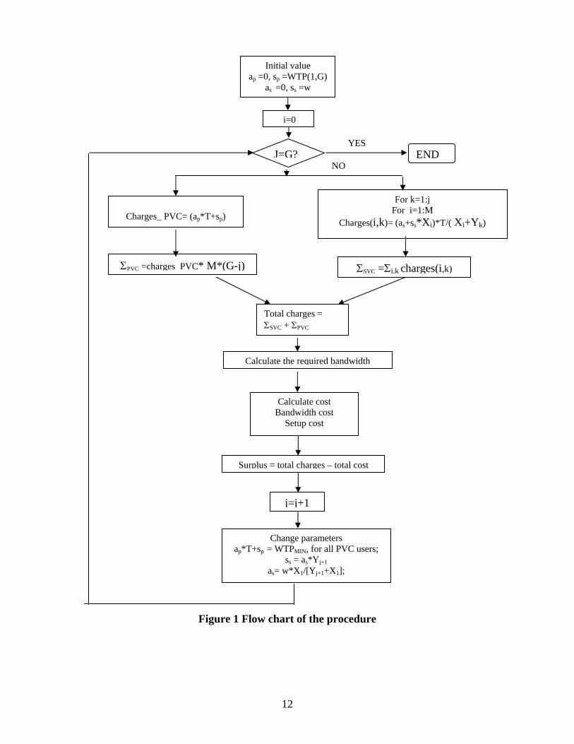
The flow chart of the procedure is given in Figure 1.

3. Results 3.1 Normalized Case

3.1.1 Parameters

In this case, we choose the normalized parameters in the following way:

• Mean ON and OFF times (time unit):

We choose the value of X of each user in the way that the average value equals 1. The

values of Y are linearly distributed within two ranges: uniformly distributed from 0 to 1

for half of the users (N/2), and uniformly distributed from 1 to 10 for the other half of the

users.

1

11

1

*

*

+

+

=

+=

jss

js

Yas

XYXw

a

11

The user number in this case is 50 (N=50), and they are divided into 10 groups with 5

users each (M=5, G=10). The users in one group have the same value of mean OFF

period (Y), but with different (X): (0.8, 0.9, 1.0, 1.1, 1.2). The values of Y are (0.2, 0.4,

0.6, 0.8, 1.0, 2, 4, 6, 8, 10).

Note: in this case the percent of SVC users will increase in steps of 10% since the

choice of service totally depends on mean OFF time. So all five users in each group will

make the same service choice.

• Bandwidth (bw):

User required bandwidth (bw) is also normalized to 1.

• Unit connection setup cost (monetary unit per connection setup):

Cost per SVC connection setup (Is): it is difficult to give the value of Is, and this

parameter affects the results dramatically, so in our results we let Is change as a variable

to show the different results under different Is.

Cost per PVC connection setup (Ip): we think it is reasonable to assume Ip to be zero.

Although there is some cost associated with this manual PVC setup, since it occurs only

once per billing period, the total PVC setup cost for the billing period is likely to be

insignificant. So unless specified, Ip equals 0.

• Unit bandwidth cost (c) (monetary unit per bandwidth unit):

This parameter is also a major factor affecting the results, so we also let it change as a

variable.

• Coefficient of willingness-to-pay (w) (monetary unit per data unit):

We normalize w to 1.

12

Figure 1 Flow chart of the procedure

Initial value ap =0, sp =WTP(1,G)

as =0, ss =w

j=0

Charges_ PVC= (ap*T+sp)

ΣPVC =charges PVC* M*(G-j)

For k=1:j For i=1:M

Charges(i,k)= (as+ss*Xi)*T/( Xi+Yk)

ΣSVC =Σi,k charges(i,k)

Total charges = ΣSVC + ΣPVC

Calculate the required bandwidth

Calculate cost Bandwidth cost

Setup cost

Surplus = total charges – total cost

Change parameters ap*T+sp = WTPMIN, for all PVC users;

ss = as*Yj+1 as= w*X1/[Yj+1+X1];

j=j+1

J=G? END YES

NO

13

(a)

(b)

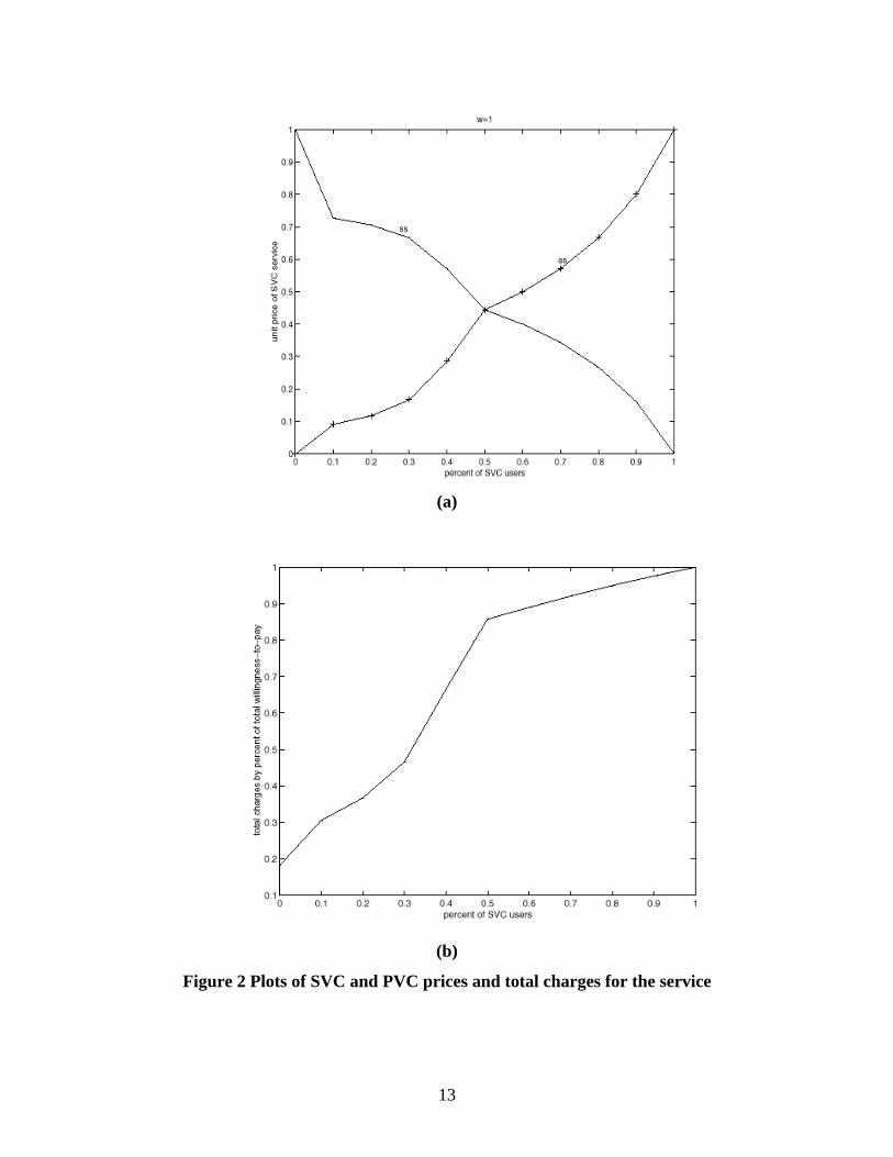
Figure 2 Plots of SVC and PVC prices and total charges for the service

14

(c)

(d)

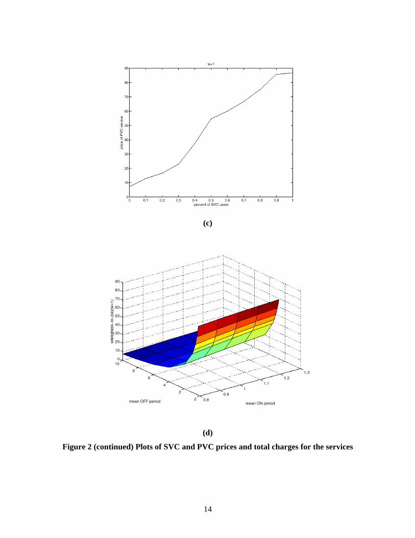
Figure 2 (continued) Plots of SVC and PVC prices and total charges for the services

15

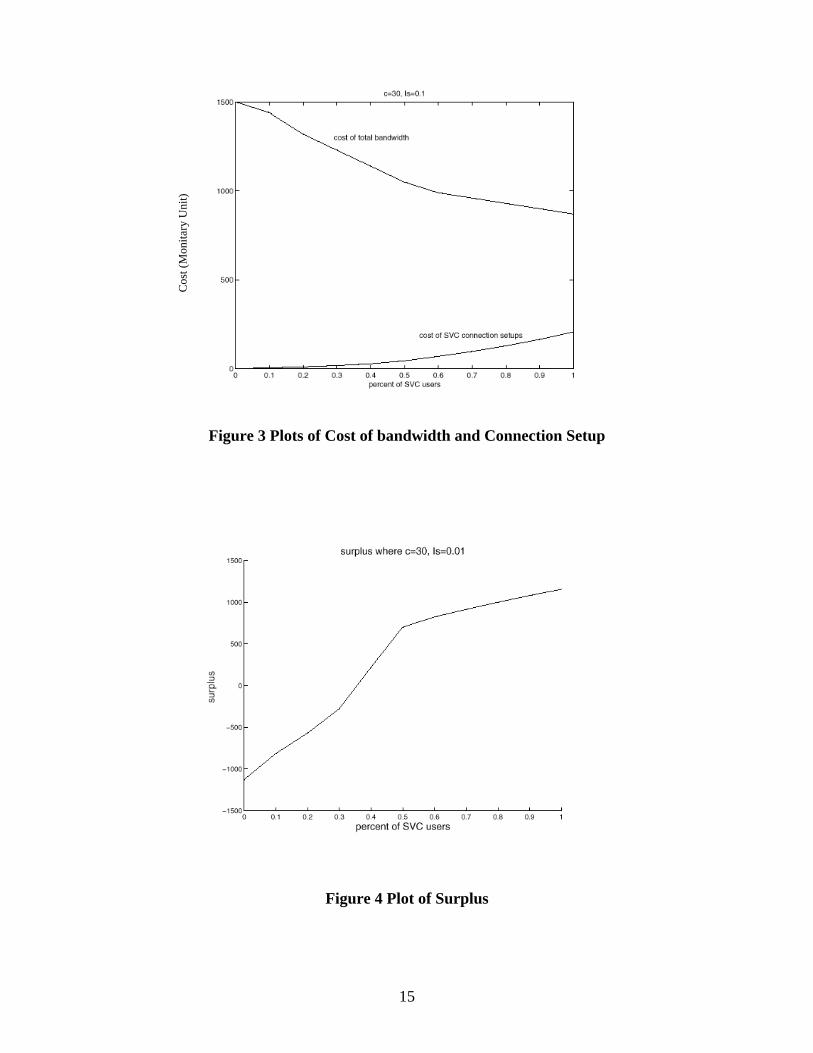
Figure 3 Plots of Cost of bandwidth and Connection Setup

Figure 4 Plot of Surplus

Cos

t (M

onita

ry U

nit)

16

3.1.2 Basic Results

Figure 2 shows the plots of SVC and PVC prices and total charges for the services vs.

the service demands in terms of percent of SVC users. As the percent of SVC users

increases, the service provider can get more revenue from the users (figure 2(b)). The

reason is that SVC service could be charged in accordance with the user’s willingness-to-

pay: the user with more traffic pays more. Notice that when all the users choose SVC

service the revenue reaches the total willingness-to-pay of all the users (at this point ss=0

and as=w).

On the other hand, PVC price is constant for all the users with diverse traffic, so it has

to be the minimum willingness to pay among the PVC users. As the result, it is beneficial

to the service provider to encourage the user with light traffic volume to choose SVC

service, so he could increase the PVC price without losing the light traffic users. In

conclusion, both the unit prices and the total PVC charges (revenue) go up as the percent

of SVC users increases (figure 2(c)). Figure 2(a) plots the unit price of SVC service for

each demand scenario. Figure 2(d) shows the willingness-to-pay of each user.

Figure 3 plots the total cost of bandwidth and connection setups vs. percent of SVC

users with c=30 and Is=0.1. It shows that the SVC service incurs more connection setup

cost, but reduces the cost of bandwidth since the service provider could achieve more

multiplexing gain with SVC service. Notice that in this case the cost of bandwidth is

higher compared with the cost of connection setups.

Figure 4 shows the surplus vs. service demands where c=30, and Is=0.1. It presents

how the trends of increasing charges, increasing connection costs, and decreasing

bandwidth interact with each other to construct the trend of surplus. The surplus begins

below 0 when all the users choose PVC; at this point the income is less than the cost of

required bandwidth. As more and more users are encouraged to choose SVC, the surplus

increases. This means the benefit from increased charges and reduced bandwidth cost

exceeds the additional costs of connection setup in this case. The optimal surplus occurs

when all the users choose SVC service.

17

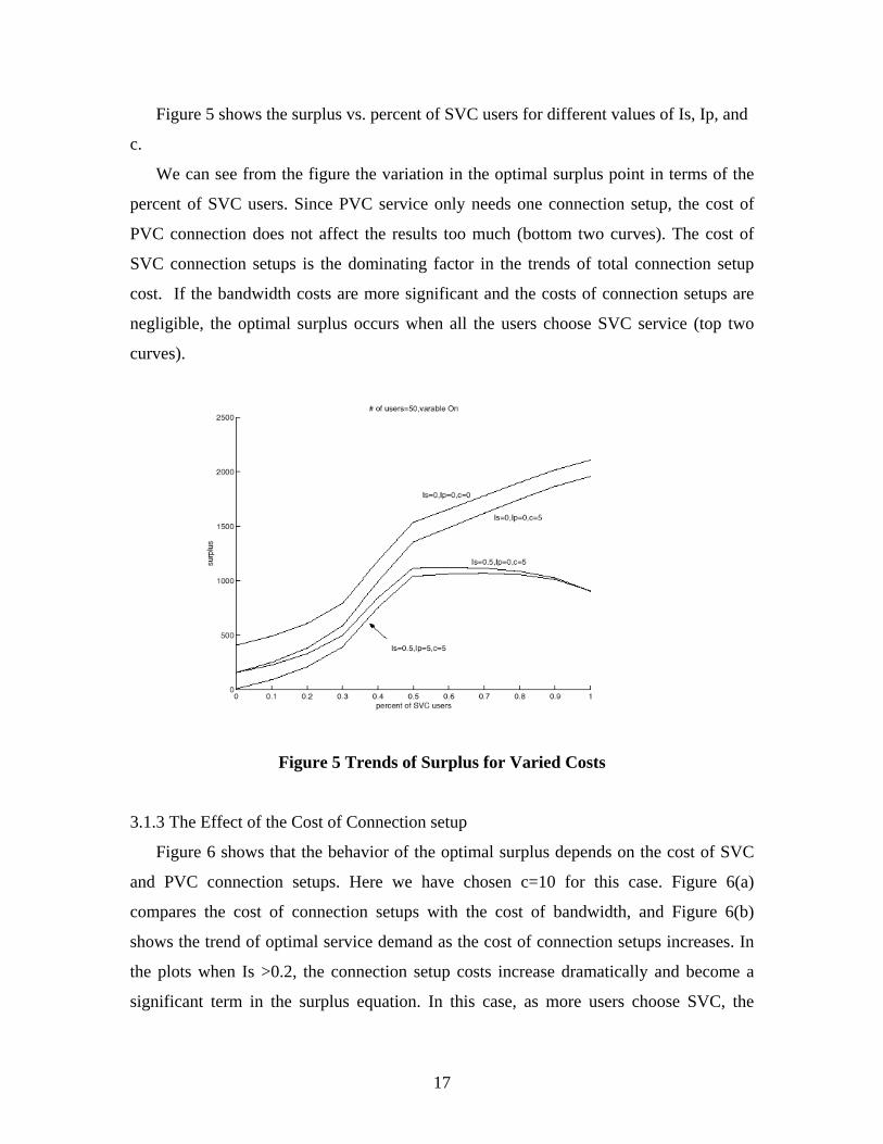
Figure 5 shows the surplus vs. percent of SVC users for different values of Is, Ip, and

c.

We can see from the figure the variation in the optimal surplus point in terms of the

percent of SVC users. Since PVC service only needs one connection setup, the cost of

PVC connection does not affect the results too much (bottom two curves). The cost of

SVC connection setups is the dominating factor in the trends of total connection setup

cost. If the bandwidth costs are more significant and the costs of connection setups are

negligible, the optimal surplus occurs when all the users choose SVC service (top two

curves).

Figure 5 Trends of Surplus for Varied Costs

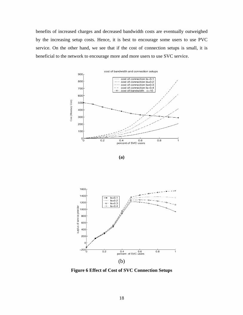
3.1.3 The Effect of the Cost of Connection setup

Figure 6 shows that the behavior of the optimal surplus depends on the cost of SVC

and PVC connection setups. Here we have chosen c=10 for this case. Figure 6(a)

compares the cost of connection setups with the cost of bandwidth, and Figure 6(b)

shows the trend of optimal service demand as the cost of connection setups increases. In

the plots when Is >0.2, the connection setup costs increase dramatically and become a

significant term in the surplus equation. In this case, as more users choose SVC, the

18

benefits of increased charges and decreased bandwidth costs are eventually outweighed

by the increasing setup costs. Hence, it is best to encourage some users to use PVC

service. On the other hand, we see that if the cost of connection setups is small, it is

beneficial to the network to encourage more and more users to use SVC service.

(a)

(b)

Figure 6 Effect of Cost of SVC Connection Setups

Cos

t (M

onita

ry U

nit)

19

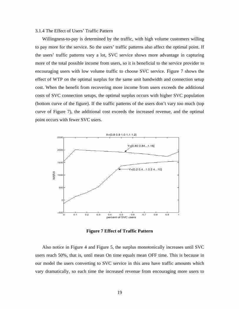
3.1.4 The Effect of Users’ Traffic Pattern

Willingness-to-pay is determined by the traffic, with high volume customers willing

to pay more for the service. So the users’ traffic patterns also affect the optimal point. If

the users’ traffic patterns vary a lot, SVC service shows more advantage in capturing

more of the total possible income from users, so it is beneficial to the service provider to

encouraging users with low volume traffic to choose SVC service. Figure 7 shows the

effect of WTP on the optimal surplus for the same unit bandwidth and connection setup

cost. When the benefit from recovering more income from users exceeds the additional

costs of SVC connection setups, the optimal surplus occurs with higher SVC population

(bottom curve of the figure). If the traffic patterns of the users don’t vary too much (top

curve of Figure 7), the additional cost exceeds the increased revenue, and the optimal

point occurs with fewer SVC users.

Figure 7 Effect of Traffic Pattern

Also notice in Figure 4 and Figure 5, the surplus monotonically increases until SVC

users reach 50%, that is, until mean On time equals mean OFF time. This is because in

our model the users converting to SVC service in this area have traffic amounts which

vary dramatically, so each time the increased revenue from encouraging more users to

20

choose SVC service exceeds the additional cost of more SVC connection setups. After

50%, the traffic changes more slowly, the benefit from SVC service grows slowly, so the

surplus can begin to decrease as the number of SVC users increases. However, as Figure

7 demonstrates, small variations in traffic patterns can result in the surplus not being

monotonically increasing up to the point (50% SVC users) at which mean ON time

equals mean OFF time.

3.1.5 Summary

Table 1 summarizes the comparison of the two services. Table 1 Cost of

Connection Setups

Cost of Bandwidth

Total Charges from Users

Situation under which the service is preferred by the provider

SVC High Low High The Cost of bandwidth is High PVC Low High Low The Cost of Connection setup is High 3.2 A Test Case

In order to verify the procedure and better understand the relationship between the

normalized parameters in our SVC vs. PVC pricing analysis, we further did a test case in

which we supply practical values to the parameters. We chose some of the parameters

from related papers, and supplied the others ourselves if we could not find anything about

them. The user traffic characteristics depend on the applications. Since web browsing is

one of the most rapidly growing applications today, we used it for our test case.

• Connection Bandwidth: We chose the value of 1Mb/s, a value appropriate for the

web browsing application, as the required bandwidth of users.

• Mean ON period length (session length): The different values of mean ON period

length (in minutes) are: 10, 12, 15, 18, 20, with the average as 15 min.

• Mean OFF period length: We let the mean value of the OFF period keep the same

relationship with mean ON length as in our previous analysis. That is, half of the values

have a uniform distribution from 1 to average mean ON length, and the other half of the

21

values are uniformly distributed from average mean ON length to 10 times the average

mean ON value.

• Cost per bandwidth unit: Reference [2] addressed the economics of statistical

multiplexing for a broadband network and calculated the cost of a broadband

transmission link. We split the cost of the transmission system over 5 years into each

month to obtain a bandwidth cost of c=$30 per Mb/s per month.

• Billing period: 1 month

• Willingness-to-pay: It’s difficult to directly calculate the willingness-to-pay of the

users, so we used the charges of current services provisioned in an ATM network as the

index to users’ willingness-to-pay. Reference [3] summarized the charging rates which

were used in the experimental project CASHMAN. We used the charge of premium web

browsing service, which is w=$0.005/Mb.

• Connection setup cost of PVC: we set Ip=0.

Our goal is to learn about the relative value of SVC connection setup cost, so we used

the other parameters as stated above to go through the procedure, searching for optimal

pricing schemes and surplus of service provider under the conditions of different unit

connection setup costs (Is). The results are shown in Figure 8.

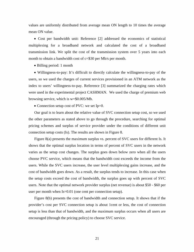
Figure 8(a) presents the maximum surplus vs. percent of SVC users for different Is. It

shows that the optimal surplus location in terms of percent of SVC users in the network

varies as the setup cost changes. The surplus goes down below zero when all the users

choose PVC service, which means that the bandwidth cost exceeds the income from the

users. While the SVC users increase, the user level multiplexing gains increase, and the

cost of bandwidth goes down. As a result, the surplus tends to increase. In this case when

the setup costs exceed the cost of bandwidth, the surplus goes up with percent of SVC

users. Note that the optimal network provider surplus (net revenue) is about $50 - $60 per

user per month when Is=0.01 (one cent per connection setup).

Figure 8(b) presents the cost of bandwidth and connection setup. It shows that if the

provider’s cost per SVC connection setup is about 1cent or less, the cost of connection

setup is less than that of bandwidth, and the maximum surplus occurs when all users are

encouraged (through the pricing policy) to choose SVC service.

22

(a)

(b)

Figure 8 Results of Test Case

Cos

t (M

onita

ry U

nit)

23

4. Further Work

ATM networks are designed to support service classes differentiated by quality of

service (QoS), so network providers are starting to provision SVC and PVC services for

different QoS service classes. In this report we did not address this issue. We simply

focused on the situation that all the users have the same quality (bandwidth) requirement.

This work could be expanded to the environment that users require different bandwidths.

In our report we did not take in account the effect of SVC connection setup time to

the user. This could be represented in a user utility function. In this case, each user

decides based on the utility function instead of only considering cost. This is a more

realistic model, so we might consider changing the model in this way to further study the

optimal pricing policy of the service provider.

References: 1. Yuhong Liu and David Petr, “The Influence of Pricing on PVC vs. SVC Service

Preference,” ITTC Technical Report ITTC-FY2000-TR-12960-03, July 1999. 2. Iraj Saniee, Ashok Erramilli, and Charles D. Pack, “The Economics of Statistical

Multiplexing for Broadband Networks,” Proceedings of International Teletraffic Congress (ITC) 15, 1997.

3. Donal Morris and Verus Pronk, “Charging for ATM Services,” IEEE Communication Magazine, May 1999.