Embed Size (px)
Citation preview
Pricing of Mexican Interest Rate Swaps inPresence of Multiple Collateral Currencies
Jorge Íñigo Martínez∗Maestría en Finanzas Cuantitativas
Facultad de Ciencias ActuarialesUniversidad Anáhuac†
Supervisor: José Luis Manrique Medina, MSc‡
March 2017
∗Email: [email protected]†Av. Universidad Anáhuac 46, Lomas Anáhuac, 52786 Huixquilucan, México.‡Universidad Anáhuac México Norte, email: [email protected]
arX
iv:1
703.
0092
3v1
[q-
fin.
PR]
2 M
ar 2
017
AbstractThe financial crisis of 2007/08 caused catastrophic consequences and brought a bunch of
changes around the world. Interest rates that were known to follow or behave similarly of eachother diverged. Furthermore, the regulation and in particular the counterparty credit risk beganto to be considered and quantified. Consequently, pre-crisis models are no longer valid. Indeed,this work sets the basis to define a valid model that considers the post-crisis world assumptionsfor the Mexican swap market. The model used in this work was the proposed by Fujii, Shimadaand Takahashi in [Fujii et al., 2010b]. This model allow us to value interest rate derivatives andfuture cash flows with the existence of a collateral agreement (with a collateral currency). Inthis document we build the discounting and projection curves for MXN interest rate derivativesconsidering the collateral currencies: USD, EUR and MXN. Also, we present the pricing whenthe derivative is uncollateralized. Finally, we show the effect of the cross-currency swaps whenvaluing through different collateral currencies.
Keywords: interest rate swap, cross-currency swap, overnight index swap, collateral, discount curve,forward curve, TIIE, LIBOR, fed funds rate
ResumenLa crisis financiera del 2007-2008 trajo consigo varias consecuencias en el mundo de las fi-
nanzas. En particular varios niveles de tasas de interés y spreads dejaron de comportarse dela forma que solían hacerlo. Además desde este evento la regulación y en particular el riesgocrediticio tomó mayor énfasis a la hora de definirlo y cuantificarlo. En consecuencia, los modelosde valuación de derivados, usados antes de la crisis, dejaron de ser válidos. Este trabajo tienecomo objetivo definir un modelo de valuación coherente que considere los supuestos del mundoactual. El modelo usado para definir la valuación de productos denominados en pesos (MXN)es el presentado por Fujii, Shimada y Takahashi en [Fujii et al., 2010b]. De hecho, este modelodemuestra que la moneda del colateral define la forma de descontar flujos de efectivo futuros enun mundo realista. En este documento se construyen las curvas para descontar flujos en pesos(MXN) cuando la moneda de colateral es: dólar americano (USD), euro (EUR) y pesos (MXN).Además, se presenta el caso de valuación cuando los swaps o en particular cualquier flujo deefectivo no tiene colateral. Finalmente se presenta un análisis de los factores que afectan a laconstrucción de curvas como los son los swaps de divisas.
Palabras clave: swap de tasa de interés, swap de divisas, swap de tasa de interés a un día, colateral,curva de descuento, curva de proyección, TIIE, LIBOR, tasa de fondos federales
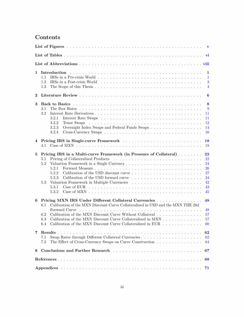
ContentsList of Figures . . . . . . . . . . . . . . . . . . . . . . . . . . . . . . . . . . . . . . . . . . . . v
List of Tables . . . . . . . . . . . . . . . . . . . . . . . . . . . . . . . . . . . . . . . . . . . . . vi
List of Abbreviations . . . . . . . . . . . . . . . . . . . . . . . . . . . . . . . . . . . . . . . . viii
1 Introduction . . . . . . . . . . . . . . . . . . . . . . . . . . . . . . . . . . . . . . . . . . . 11.1 IRSs in a Pre-crisis World . . . . . . . . . . . . . . . . . . . . . . . . . . . . . . . . . . 11.2 IRSs in a Post-crisis World . . . . . . . . . . . . . . . . . . . . . . . . . . . . . . . . . 31.3 The Scope of this Thesis . . . . . . . . . . . . . . . . . . . . . . . . . . . . . . . . . . . 4
2 Literature Review . . . . . . . . . . . . . . . . . . . . . . . . . . . . . . . . . . . . . . . . 6
3 Back to Basics . . . . . . . . . . . . . . . . . . . . . . . . . . . . . . . . . . . . . . . . . . 83.1 The Ibor Rates . . . . . . . . . . . . . . . . . . . . . . . . . . . . . . . . . . . . . . . . 93.2 Interest Rate Derivatives . . . . . . . . . . . . . . . . . . . . . . . . . . . . . . . . . . . 11
3.2.1 Interest Rate Swaps . . . . . . . . . . . . . . . . . . . . . . . . . . . . . . . . . 113.2.2 Tenor Swaps . . . . . . . . . . . . . . . . . . . . . . . . . . . . . . . . . . . . . 123.2.3 Overnight Index Swaps and Federal Funds Swaps . . . . . . . . . . . . . . . . . 143.2.4 Cross-Currency Swaps . . . . . . . . . . . . . . . . . . . . . . . . . . . . . . . . 16
4 Pricing IRS in Single-curve Framework . . . . . . . . . . . . . . . . . . . . . . . . . . 184.1 Case of MXN . . . . . . . . . . . . . . . . . . . . . . . . . . . . . . . . . . . . . . . . . 18
5 Pricing IRS in a Multi-curve Framework (in Presence of Collateral) . . . . . . . . 225.1 Pricing of Collateralized Products . . . . . . . . . . . . . . . . . . . . . . . . . . . . . 225.2 Valuation Framework in a Single Currency . . . . . . . . . . . . . . . . . . . . . . . . . 24
5.2.1 Forward Measure . . . . . . . . . . . . . . . . . . . . . . . . . . . . . . . . . . . 265.2.2 Calibration of the USD discount curve . . . . . . . . . . . . . . . . . . . . . . . 275.2.3 Calibration of the USD forward curve . . . . . . . . . . . . . . . . . . . . . . . 34
5.3 Valuation Framework in Multiple Currencies . . . . . . . . . . . . . . . . . . . . . . . 425.3.1 Case of EUR . . . . . . . . . . . . . . . . . . . . . . . . . . . . . . . . . . . . . 435.3.2 Case of MXN . . . . . . . . . . . . . . . . . . . . . . . . . . . . . . . . . . . . . 45
6 Pricing MXN IRS Under Different Collateral Currencies . . . . . . . . . . . . . . . 486.1 Calibration of the MXN Discount Curve Collateralized in USD and the MXN TIIE 28d
Forward Curve . . . . . . . . . . . . . . . . . . . . . . . . . . . . . . . . . . . . . . . . 486.2 Calibration of the MXN Discount Curve Without Collateral . . . . . . . . . . . . . . . 576.3 Calibration of the MXN Discount Curve Collateralized in MXN . . . . . . . . . . . . . 576.4 Calibration of the MXN Discount Curve Collateralized in EUR . . . . . . . . . . . . . 60
7 Results . . . . . . . . . . . . . . . . . . . . . . . . . . . . . . . . . . . . . . . . . . . . . . . 627.1 Swap Rates through Different Collateral Currencies . . . . . . . . . . . . . . . . . . . . 627.2 The Effect of Cross-Currency Swaps on Curve Construction . . . . . . . . . . . . . . . 64
8 Conclusions and Further Research . . . . . . . . . . . . . . . . . . . . . . . . . . . . . 67
References . . . . . . . . . . . . . . . . . . . . . . . . . . . . . . . . . . . . . . . . . . . . . . . 68
Appendices . . . . . . . . . . . . . . . . . . . . . . . . . . . . . . . . . . . . . . . . . . . . . . 71
iii
A Proofs . . . . . . . . . . . . . . . . . . . . . . . . . . . . . . . . . . . . . . . . . . . . . . . 71A.1 Proof of Theorem 5.3 . . . . . . . . . . . . . . . . . . . . . . . . . . . . . . . . . . . . . 71
B Conventions & Calendars . . . . . . . . . . . . . . . . . . . . . . . . . . . . . . . . . . . 72B.1 Day Count Conventions . . . . . . . . . . . . . . . . . . . . . . . . . . . . . . . . . . . 72B.2 Date Rolling Conventions . . . . . . . . . . . . . . . . . . . . . . . . . . . . . . . . . . 72B.3 Calendars . . . . . . . . . . . . . . . . . . . . . . . . . . . . . . . . . . . . . . . . . . . 72
C Methods of Interpolation . . . . . . . . . . . . . . . . . . . . . . . . . . . . . . . . . . . 74C.1 Linear Interpolation on Yield Curve . . . . . . . . . . . . . . . . . . . . . . . . . . . . 74C.2 Linear Interpolation on Log Discount Factors . . . . . . . . . . . . . . . . . . . . . . . 75C.3 Natural Cubic Splines Interpolation on Yield Curve . . . . . . . . . . . . . . . . . . . 75
D Example of a Bootstrapping Algorithm (OIS Curve) . . . . . . . . . . . . . . . . . . 79
E Bloomberg & SuperDerivatives Data . . . . . . . . . . . . . . . . . . . . . . . . . . . . 80
iv
List of Figures1.1 Example of an IRS . . . . . . . . . . . . . . . . . . . . . . . . . . . . . . . . . . . . . . 21.2 LIBOR-OIS 3m Spread (2001-2015) . . . . . . . . . . . . . . . . . . . . . . . . . . . . 34.1 TIIE 28d yield curve in a single-curve framework . . . . . . . . . . . . . . . . . . . . . 204.2 TIIE 28d discount curve in a single-curve framework . . . . . . . . . . . . . . . . . . . 214.3 TIIE 28d forward curve in a single-curve framework . . . . . . . . . . . . . . . . . . . 215.2 OIS Yield Curve . . . . . . . . . . . . . . . . . . . . . . . . . . . . . . . . . . . . . . . 325.3 OIS Discount Curve . . . . . . . . . . . . . . . . . . . . . . . . . . . . . . . . . . . . . 325.4 OIS 1d-Forward Curve . . . . . . . . . . . . . . . . . . . . . . . . . . . . . . . . . . . . 335.5 FOMC Meetings, OIS forward curve and FOMC monetary policy scenario . . . . . . . 345.6 LIBOR 1m 1m-Forward Curve . . . . . . . . . . . . . . . . . . . . . . . . . . . . . . . 405.7 LIBOR 1m Yield Curve . . . . . . . . . . . . . . . . . . . . . . . . . . . . . . . . . . . 405.8 LIBOR 1m Discount Curve . . . . . . . . . . . . . . . . . . . . . . . . . . . . . . . . . 415.9 Flowchart for curve construction: differences between EUR and MXN curves when the
collateral currency is USD . . . . . . . . . . . . . . . . . . . . . . . . . . . . . . . . . . 476.1 MXN discount curve collateralized in USD (multi-curve framework) . . . . . . . . . . 556.2 Comparison of MXN discount curves in a multi-curve framework . . . . . . . . . . . . 566.3 TIIE 28d forward curve in a multi-curve framework . . . . . . . . . . . . . . . . . . . . 566.4 Comparison of TIIE 28d forward curve in a multi-curve framework . . . . . . . . . . . 576.5 Overnight Rate (Fondeo Bancario) and Interbank Offered Rate (TIIE 28d) during the
period 2008-2015. . . . . . . . . . . . . . . . . . . . . . . . . . . . . . . . . . . . . . . . 586.6 Spread between the Overnight Rate (Fondeo Bancario) and the Interbank Offered Rate
(TIIE 28d) during the period 2008-2015. . . . . . . . . . . . . . . . . . . . . . . . . . . 596.7 Spread between the Overnight Rate (Fondeo Bancario) and the Interbank Offered Rate
(TIIE 28d) during the period 2014-2015. . . . . . . . . . . . . . . . . . . . . . . . . . . 597.1 MXN Discount Curves in different collateral currencies . . . . . . . . . . . . . . . . . . 637.2 The Effect of XCSs in the Mexican Swap Market . . . . . . . . . . . . . . . . . . . . . 647.3 The Effect of XCSs in the TIIE 28d Forward Curve . . . . . . . . . . . . . . . . . . . . 657.4 The Effect of XCSs in the Discount Curve . . . . . . . . . . . . . . . . . . . . . . . . . 657.5 The Effect of cnXCSs: USD-collateralized vs uncollateralized swaps . . . . . . . . . . . 667.6 The Effect of cnXCSs: USD-collateralized vs MXN-collateralized swaps . . . . . . . . 66
v
List of Tables3.1 Term sheet sample of a plain vanilla IRS based on TIIE 28d with maturity of 5y. . . . 123.2 Example of a plain vanilla 5y tenor swap contract. . . . . . . . . . . . . . . . . . . . . 143.3 Example of a plain vanilla OIS 5y contract linked to Fed Funds Overnight Rate. . . . 153.4 Example of a plain vanilla OIS 2y contract linked to Eonia Overnight Rate. . . . . . . 163.5 Example of a plain vanilla mtmXCS EURUSD 5y Contract. . . . . . . . . . . . . . . . 173.6 Example of a plain vanilla cnXCS 10y Contract. . . . . . . . . . . . . . . . . . . . . . 174.1 Quoted TIIE 28D Swaps (%) on May 29 2015 (Source: Bloomberg). Every swap trades
with the convention of 28 days Following with accrual period of ACT/360. . . . . . . . 195.1 Quoted USD OIS (%) on May 29 2015 (Source: Bloomberg). ∗The 18m OIS swap
convention has an upfront short stub, i.e., each leg has two coupons: the first with anaccrual period of 6M and the second with an accrual period of 12m (1m). . . . . . . . 30
5.2 SuperDerivatives market data of the USD Tenor Swaps (1mv3m, 3mv6m, 3mv12m)(see Section 5.2.3). Quotes are End of Day prices from May 29, 2015. The quotes weretaken from www.superderivatives.com on June 21, 2015. . . . . . . . . . . . . . . . . 37
6.1 Quoted TIIE 28d IRSs and USDMXN cnXCSs on May 29 2015 (Source: Bloomberg). 507.1 Par Swap Rates of IRSs based on TIIE 28d with different collateral currencies. . . . . 627.2 Differences in basis points based on USD-collateralized par swap rates. . . . . . . . . . 637.3 In this table we present the values of the cnXCS basis spreads that we use for the
analysis if the effect . . . . . . . . . . . . . . . . . . . . . . . . . . . . . . . . . . . . . . 64E.1 SuperDerivatives market data of the USD OIS Swap Curve (see Section 5.2.2). Quotes
are End of Day prices fromMay 29, 2015. The quotes were taken from www.superderivatives.com on June 21, 2015. ∗The 18m OIS swap convention has an upfront short stub, i.e.,each leg has two coupons: the first with an accrual period of 6m and the second withan accrual period of 12m (1y). . . . . . . . . . . . . . . . . . . . . . . . . . . . . . . . 80
E.2 In this table, we present the Bloomberg market data used for the construction of theUSD discount curve (see Section 5.2.2). Quotes are End of Day prices from May 29,2015. The quotes were taken from a Bloomberg Terminal on June 21, 2015. ∗The 18mOIS swap convention has an upfront short stub, i.e., each leg has two coupons: the firstwith an accrual period of 6m and the second with an accrual period of 12m (1y). . . . 81
E.3 SuperDerivatives market data of the USD LIBOR 3m Swap Curve (see Section 5.2.3).Quotes are End of Day prices from May 29, 2015. The quotes were taken from www.superderivatives.com on June 21, 2015. . . . . . . . . . . . . . . . . . . . . . . . . . 82
E.4 SuperDerivatives market data of the USD LIBOR 1m Swap Curve (see Section 5.2.3).Quotes are End of Day prices from May 29, 2015. The quotes were taken from www.superderivatives.com on June 21, 2015. . . . . . . . . . . . . . . . . . . . . . . . . . 83
E.5 In this table, we present the Bloomberg market data used for the construction of theLIBOR 3m forward curve (see Section 5.2.3). Quotes are End of Day prices from May29, 2015. The quotes were taken from a Bloomberg Terminal on June 21, 2015. . . . . 84
E.6 In this table, we present the Bloomberg market data used for the construction of theLIBOR 1m forward curve (see Section 5.2.3). Recall that plain vanilla TSs (LIBOR1m vs LIBOR 3m) have a payment frequency of 3 months (quarterly) for both legs.However, in the LIBOR 1m leg, the fixing resets on a monthly basis and then is com-pounded to define the quarterly payment. Quotes are End of Day prices from May 29,2015. The quotes were taken from a Bloomberg Terminal on June 21, 2015. . . . . . . 85
E.7 SuperDerivatives market data of the USDMXN Cross-Currency Swaps (Constant No-tional). Quotes are End of Day prices from May 29, 2015. The quotes were taken fromwww.superderivatives.com on June 21, 2015. . . . . . . . . . . . . . . . . . . . . . . 86
vi
E.8 SuperDerivatives market data of the TIIE 28d Swap Curve. Quotes are End of Dayprices from May 29, 2015. The quotes were taken from www.superderivatives.comon June 21, 2015. . . . . . . . . . . . . . . . . . . . . . . . . . . . . . . . . . . . . . . . 86
E.9 In this table, we present the Bloomberg market data of the TIIE 28d IRSs used forthe construction of the MXN-discount curve (collateralized in USD) and the TIIE 28dforward curve. Quotes are End of Day prices from May 29, 2015. The quotes weretaken from a Bloomberg Terminal on June 21, 2015. . . . . . . . . . . . . . . . . . . . 87
E.10 In this table, we present the Bloomberg market data of the USDMXM cnCXS usedfor the construction of the MXN-discount curve (collateralized in USD) and the TIIE28d forward curve. Quotes are End of Day prices from May 29, 2015. The quotes weretaken from a Bloomberg Terminal on June 21, 2015. . . . . . . . . . . . . . . . . . . . 88
vii
List of AbbreviationsBS: Black and Scholes
EUR: Euro code (ISO 4217)
USD: United States Dollar code (ISO 4217)
MXN: Mexican Peso code (ISO 4217)
JPY: Japanese Yen code (ISO 4217)
FX: Foreign Exchange
IRS: Interest Rate Swap
TS: Tenor Swap
OIS: Overnight Index Swap
FFS: Federal Funds Swap
XCS: Cross-Currency Swap
cnXCS: Constant Notional Cross-Currency Swap
mtmXCS: Mark-to-Market Cross-Currency Swap
OTC: Over The Counter
IBOR: Interbank Offered Rate
LIBOR: London Interbank Offered Rate
EURIBOR: European Interbank Offered Rate
TIIE: Tasa de Interés Interbancaria de Equilibrio
PV: Net Present Value
ISDA: International Swaps and Derivatives Association
CSA: Credit Support Annex
CVA: Credit Valuation Adjustment
viii
1 Introduction
1 IntroductionSince the publication of the well-known and famous paper [Black and Scholes, 1973], the theory re-garding the pricing of derivative securities has been developed through the time using this seminalpaper as a main basis. Among all the papers published by these authors, Fischer Black and MyronScholes, between 1973 and 1977, there were many assumptions that simplified1 their Black-Scholes(BS) model [Hens and Rieger, 2010], such as:
Trading in the assets is continuous in timeThe market is arbitrage freeThere is a constant risk-free rate for which banks can borrow and lend money (no limit amount!)There are no short-selling constraintsThere are no frictions, like transaction costs and taxesThere is no dividend paymentsNeither counterparty to the transaction is at risk of default
It is important to point out that even in the mid-1970s, Black and Scholes were aware that theirassumptions did (and do) not reflect the financial markets reality. Since then, these assumptionshave been weakened by researchers with post-BS model papers suggesting modifications of the BSformula. For instance, in 1973, Robert C. Merton [Merton, 1973] removed the restriction of constantinterest rates; in 1977, Jonathan Ingersoll [Ingersoll, 1977] relaxed the assumption of no taxes andtransaction costs; in 1979, John Cox, Stephen Ross and Mark Rubinstein [Cox et al., 1979] presenteda model that incorporates the timing and size of dividend payments.
Aside from these papers with variations of the BS model, derivatives valuation theory has beenan active and popular research topic in financial engineering for both industry and academia. Indeed,many banks and financial institutions have been investing large amounts of money in research anddevelopment of software used for numerical calculations and simulations for pricing and risk manage-ment of derivatives. However, another major event —and perhaps the most important— that markeda milestone in the history of derivatives valuation was the Lehman Brothers collapse in 2008.
The financial crisis in 2007-2008 arose problems in many latitudes such as public policy, monetarypolicy and regulation of financial markets, without mentioning the historical plunge of stock mar-kets and the paralysis of credit markets. Financial engineering was not exempt of the crisis. In fact,derivatives valuation frameworks entered on a process of changes in methodology and assumptions.To illustrate some of these changes we will present how the typical variables, considered for pricinga plain vanilla interest rate swap2 (IRS) in a pre-crisis world, have changed notably in a post-crisisworld. This comparison was mostly taken from [Green, 2015] among other references cited below.
1.1 IRSs in a Pre-crisis WorldBefore we analyze the main characteristics of IRSs in a pre-crisis world, let us explain briefly whyswaps have become popular instruments. Around the world, companies and institutions typicallyown debt linked to interest rates (fixed or floating). Since there exist a lot of uncertainty about futureinterest rates levels, swaps allow them to hedge their interest rate exposures by exchanging a fixedrate for a floating rate, typically an Ibor3 rate, or vice versa. To illustrate this we present the followingexample in which a company uses an IRS to hedge its position.
1The word simplify is used in an academic context, i.e. in a critical and not in a derogatory way.2Interest rate swaps (IRS) can be divided in three main types; plain vanilla IRS where two parties exchange fixed
and floating rate payments, the tenor swap (TS) where they exchange interest rate payments based on different floatingreference rates of the same currency and the cross-currency swap (XCS) where they exchange floating interest ratepayments in two different currencies. See section 3.2.
3By Ibor (Interbank offered rate) we mean any reference rate which is fixed in a way similar to LIBOR, EURIBOR,TIBOR, TIIE, etc. See section 3.1
1
1 Introduction
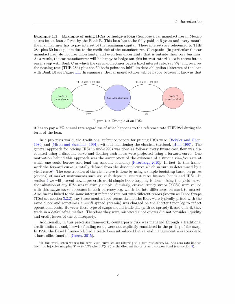
Example 1.1. (Example of using IRSs to hedge a loan) Suppose a car manufacturer in Mexicoenters into a loan offered by the Bank B. This loan has to be fully paid in 5 years and every monththe manufacturer has to pay interest of the remaining capital. These interests are referenced to TIIE28d plus 50 basis points due to the credit risk of the manufacturer. Companies (in particular the carmanufacturer) do not like uncertainty, and even less uncertainty that is outside their core business.As a result, the car manufacturer will be happy to hedge out this interest rate risk, so it enters into apayer swap with Bank C in which the car manufacturer pays a fixed interest rate, say 7%, and receivesthe floating rate (TIIE 28d) plus the 50 basis points to fulfill its debt obligation (interests of the loanwith Bank B) see Figure 1.1. In summary, the car manufacturer will be happy because it knowns that
Car ManufacturerBank C
(swap dealer)Bank B
(moneylender)
Loan
TIIE 28d + 50 bps TIIE 28d + 50 bps
7%
Figure 1.1: Example of an IRS.
it has to pay a 7% annual rate regardless of what happens to the reference rate TIIE 28d during theterm of the loan.
In a pre-crisis world, the traditional reference papers for pricing IRSs were [Bicksler and Chen,1986] and [Miron and Swannell, 1991], without mentioning the classical textbook [Hull, 1997]. Thegeneral approach for pricing IRSs in mid-1990s was done as follows: every future cash flow was dis-counted using a discount curve and floating cash flows were projected using a forward curve. Onemotivation behind this approach was the assumption of the existence of a unique risk-free rate atwhich one could borrow and lend any amount of money [Piterbarg, 2010]. In fact, in this frame-work the forward curve is totally defined from the discount curve which in turn is determined by ayield curve4. The construction of the yield curve is done by using a simple bootstrap based on prices(quotes) of market instruments such as: cash deposits, interest rates futures, bonds and IRSs. Insection 4 we will present how a pre-crisis world simple bootstrapping is done. Using this yield curve,the valuation of any IRSs was relatively simple. Similarly, cross-currency swaps (XCSs) were valuedwith this single-curve approach in each currency leg, which led into differences on mark-to-market.Also, swaps linked to the same interest reference rate but with different tenors (known as Tenor Swaps(TSs) see section 3.2.2), say three months Ibor versus six months Ibor, were typically priced with thesame quote and sometimes a small spread (premia) was charged on the shorter tenor leg to reflectoperational costs. However these type of swaps should trade flat (with no spread) if, and only if, theytrade in a default-free market. Therefore they were mispriced since quotes did not consider liquidityand credit issues of the counterparty.
Additionally, in this pre-crisis framework, counterparty risk was managed through a traditionalcredit limits set and, likewise funding costs, were not explicitly considered in the pricing of the swap.In 1996, the Basel I framework had already been introduced but capital management was considereda back office function [Green, 2015].
4In this work, when we use the term yield curve we are referring to a zero rate curve, i.e. the zero rate impliedfrom the injective mapping T 7→ P (t, T ) where P (t, T ) is the discount factor or zero coupon bond (see section 3).
2
1 Introduction
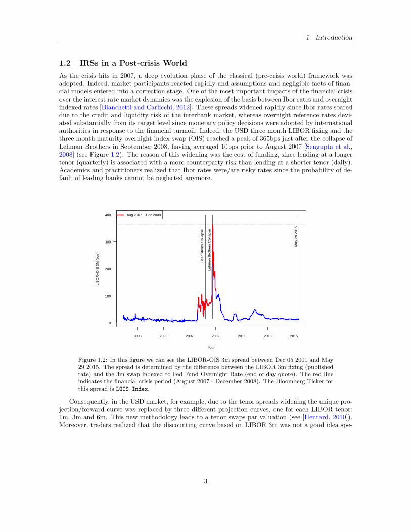
1.2 IRSs in a Post-crisis WorldAs the crisis hits in 2007, a deep evolution phase of the classical (pre-crisis world) framework wasadopted. Indeed, market participants reacted rapidly and assumptions and negligible facts of finan-cial models entered into a correction stage. One of the most important impacts of the financial crisisover the interest rate market dynamics was the explosion of the basis between Ibor rates and overnightindexed rates [Bianchetti and Carlicchi, 2012]. These spreads widened rapidly since Ibor rates soareddue to the credit and liquidity risk of the interbank market, whereas overnight reference rates devi-ated substantially from its target level since monetary policy decisions were adopted by internationalauthorities in response to the financial turmoil. Indeed, the USD three month LIBOR fixing and thethree month maturity overnight index swap (OIS) reached a peak of 365bps just after the collapse ofLehman Brothers in September 2008, having averaged 10bps prior to August 2007 [Sengupta et al.,2008] (see Figure 1.2). The reason of this widening was the cost of funding, since lending at a longertenor (quarterly) is associated with a more counterparty risk than lending at a shorter tenor (daily).Academics and practitioners realized that Ibor rates were/are risky rates since the probability of de-fault of leading banks cannot be neglected anymore.
0
100
200
300
400
Year
LIB
OR
−O
IS 3
M (
bps)
2003 2005 2007 2009 2011 2013 2015
May
29
2015
Lehm
an B
roth
ers
Col
laps
e
Bea
r S
tern
s C
olla
pse
Aug 2007 − Dec 2008
Figure 1.2: In this figure we can see the LIBOR-OIS 3m spread between Dec 05 2001 and May29 2015. The spread is determined by the difference between the LIBOR 3m fixing (publishedrate) and the 3m swap indexed to Fed Fund Overnight Rate (end of day quote). The red lineindicates the financial crisis period (August 2007 - December 2008). The Bloomberg Ticker forthis spread is LOIS Index.
Consequently, in the USD market, for example, due to the tenor spreads widening the unique pro-jection/forward curve was replaced by three different projection curves, one for each LIBOR tenor:1m, 3m and 6m. This new methodology leads to a tenor swaps par valuation (see [Henrard, 2010]).Moreover, traders realized that the discounting curve based on LIBOR 3m was not a good idea spe-
3
1 Introduction
cially for trades under Credit Support Annex5 (CSA) agreements. In fact, CSA agreements pay aninterest rate on posted collateral typically equal to an overnight rate of the collateral currency. There-fore markets migrated rapidly to the usage of overnight rates for discounting collateralized cash flowsof interest rate derivatives [Piterbarg, 2010]. The incorporation of tenor basis spreads and collateralrates forced to create a valuation framework that considers multiple rate curves known as multi-curveframework.
Furthermore in a post-crisis world, credit and liquidity costs have started to be considered whenswaps are priced. Indeed, CVA (Credit Valuation Adjustment) and FVA (Funding Valuation Adjust-ment) variables should be made for quantifying the costs of credit and funding of unsecured derivativetransactions. In addition, capital management is no longer a back office function. Capital require-ments are now an expensive resource that front office has to manage carefully as core activity. Henceevery new transaction offered to the clients has to be priced considering the cost of capital, in orderto determine whether it is profitable or not. This cost of capital is know as KVA (Capital ValuationAdjustment).
In summary, in a post-crisis world for the valuation of an IRS we need to consider a large number ofinterest rate instruments (cash deposits, futures, IRSs, XCSs, foreign exchange swaps, etc.) to fulfillmultiple bootstrappings for projections and discounting curves and also we have to perform Monte-Carlo simulations for every counterparty to manage and calculate XVA variables: CVA (DVA)6, FVA,KVA and MVA (Margin Valuation Adjustment). For further references in XVA variables we invitethe reader to check [Gregory, 2012], [Green, 2015], [Ruiz, 2015] and [Lichters et al., 2015].
In this thesis we will focus on the construction of the discount and forward curves in presenceof a CSA agreement (collateral agreements) through different currencies. It is important to statethat the transition away from risk-neutral valuation framework (pre-crisis world) to a more realisticvaluation framework (post-crisis world) is not yet completed. Therefore the reader should know thatthe methodology presented here is not definitely and can be modified through the time once the rulesof the game change or more assumptions start to weaken.
1.3 The Scope of this ThesisThe aim of this work is to describe the construction under discount and projection curves used for thevaluation of IRSs in MXN currency (Mexican Peso) for different collateral currencies such as: USD,MXN and EUR. Also we will explain how to price uncollateralized IRSs and how the multi-curveframework affects IRSs in the absence of a collateral agreement. This work is a novelty since thereare not known publications that take into account curve construction in a market where overnightindex swaps do not exist. Furthermore, this could be considered a theoretical extension of the whitepaper Análisis Comparativo de las Metodologías de Valuación de Swaps de TIIE [MexDer, 2014] pub-lished by Mexican Derivatives Exchange (MexDer)7 in 2014. Moreover we will justify mathematicallyevery step and also to present explicit formulas for pricing IRSs. Finally this thesis distinguishes from[MexDer, 2014] since we detail all steps to compute a dual (or multiple) bootstrapping.
This thesis is structured as follows: in section 2 we summarize a brief literature review of themain publications that manage topics such as: curve construction with collateral, bootstrapping andinterpolation of curves. In section 3 we begin with the most basic concepts in mathematical finance
5A Credit Support Annex (CSA), is a legal document which regulates credit support (collateral) for derivativetransactions. It is one of the four parts that make up an ISDA (International Swaps and Derivatives Association) MasterAgreement but is not mandatory. CSAs are characterized by various clauses and parameters, such as marginationfrequency, margination rate, threshold, minimum transfer amount, eligible collateral, collateral currency, asymmetry,etc. See section 5.1.
6In a bilateral model, DVA (Debt Valuation Adjustment) is considered a mirror of CVA since the valuation adjust-ment has to be symmetric among counterparties.
7The Mexican Derivatives Exchange (MexDer) is an options and futures exchange in Mexico, located in the samebuilding as the Mexican Stock Exchange (Bolsa Mexicana de Valores, BMV) and a subsidiary of the same owninggroup.
4

1 Introduction
i.e. discount factors, yield curves, forward rate, zero rates and how to use a rate curve. Additionallywe introduce financial products such as IRSs, TSs, OISs and XCSs. In section 4 we explain the pre-crisis methodology for pricing IRSs in the MXN market and describe formally every formula and thesteps to perform a bootstrapping. Section 5 is divided in three subsections. At the beginning of thesection we summarize the general collateral valuation framework considered in [Fujii et al., 2010b] and[Piterbarg, 2010]. In the second subsection we present the curve construction of IRSs and OISs whenthe currency of the swap and the collateral currency are the same, detailing explicitly formulas for thecalibration of the OIS-discount curve and LIBOR 1m forward curve in the USD market. In the thirdsubsection we discuss the case when the payoffs currency of the swaps are different from the collateralcurrency, also we explain briefly the difference between pricing IRSs based on EUR and MXN whenthe collateral is posted in USD. Then we analyze why liquidity in the market and the non-existence ofan overnight swap market affects the MXN interest rate curves construction. In section 6 we developthe main formulas and methodology for the valuation and pricing of MXN IRSs based on TIIE 28dwith multiple collateral currencies, such as: in USD, MXN, EUR and non collateralized contracts.In section 7 we present the main results of the thesis; first we show the historical differences in swaprates considering the collateral currencies and we also analyze how the size of the spread of XCSsaffects the differences of swap rates in each collateral currency. Finally in section 8 we present ourconclusions and further research to manage better the curve calibration in distinct currencies.
5
2 Literature Review
2 Literature ReviewAs we saw in the introduction, throughout this work we will entirely focus on the construction ofinterest rate curves in presence of collateral. Fortunately for the mathematical finance theory, theconstruction of interest rates curves has been an active area of research in both the industry andacademia. A great variety of papers and research documents have been published treating rate curveconstruction through different currencies, mostly for EUR, USD and JPY (Japanese Yen) curren-cies. However, as in all mathematical finance research topic, most of the statistical and mathematicalmodels that are applied in the industry are developed in-house and typically are not published foracademic purposes. Nonetheless, across this section, we will survey some of the available literaturefor pricing collateralized interest rates swaps. This literature review has been organized into threemain parts. First, the main papers treating curves construction in a multi-curve framework with theincorporation of collateral are explored. Secondly we discuss the evolution of the papers published byMasaaki Fujii, Yasufumi Shimada and Akihiko Takahashi8 [Fujii et al., 2010a], [Fujii et al., 2010b],[Fujii and Takahashi, 2015a], followed by the applications of this framework through multiple cur-rencies such as EUR, JPY and SEK (Swedish Krona). It is important to point out that [Fujii et al.,2010b] is our main reference and almost all the theory involved in this work is based on it. Finallywe examine the basic literature for interpolation and bootstrapping methods.
The post-crisis world brought to financial theory a multi-curve framework which is nowadays thestandard pricing framework. In terminology, the multi-curve characteristics plus the existence of col-laterals through CSA agreements, has often been reduced to the term OIS-discounting. However, wewill not use this term since the property of using an overnight rate as collateral rate is just one ofthe characteristics of the multi-curve framework. One of the first papers that explores a multi-curveframework without collateral was [Henrard, 2007]. In this publication, the author questioned the wayderivatives cash flows were discounted. He realized that, since counterparties have different credit rat-ings or default risks, each of them must have associated a unique discount curve for the pricing of itsderivatives position. Nevertheless, in practice, for a counterparty who traded an OIS and a IRS basedon LIBOR, different discounting curves were often used for the valuation of the mark-to-markets. In-deed, the IRS cash flows were valued using a discount curve implied from the LIBOR curve, whereasthe OIS used an implied LIBOR − 12.5bps (≈ Fed Funds rate) curve. In 2010 the author publisheda second part of this publication ([Henrard, 2010]), he wrote that ironically his work [Henrard, 2007]was published in July 2007, just one month before the financial turmoil which leaded to the wideningof LIBOR-OIS spread. Many other papers were published after the crisis to enhance the theory behindmulti-curve frameworks. In [Bianchetti, 2008], the multi-curve framework is presented for pricing co-herently IRS taking into account the forward basis spread taken from the TSs market. In [Pallaviciniand Tarenghi, 2010] the authors explore market evidences through swaptions and contant maturityswaps (CMSs) quoted in the market that suggest the existence of multiple yield curves that avoidsarbitrage among products. In [Ametrano and Bianchetti, 2013], the authors discuss the multi-curveframework in a detailed way. They present the EUR market case, specifically which products haveto be considered for the construction of multiple curves, how to perform bootstrappings and how tocompute delta sensitivities.
The model that we will discuss in this thesis is completely based on [Fujii et al., 2010b]. In thisfamous paper, Fujii, Shimada and Takahashi explain the method to construct multiple swap curvesconsistently with all the relevant swaps, say IRSs, TSs, XCSs, with and without a collateral agree-ment. They also consider the method to construct the term structures of collateralized swaps in themulti-currency setup. They present formulas that could be used for pricing swaps in USD and JPYcurrencies. In a later published article [Fujii et al., 2010a], they show the importance of the choice ofcollateral currency. They discuss the implications in market risk management when derivative con-tracts allow multiple currencies as eligible collateral and a free replacement among them. In their
8University of Tokyo, Faculty of Economics
6
2 Literature Review
more recent papers [Fujii and Takahashi, 2015a] and [Fujii and Takahashi, 2015b], they extend theirprevious works. In particular they develop a formulation for the funding spread dynamics which ismore suitable in the presence of non-zero correlation to the collateral rates. In [Gunnarsson, 2013]the author implements the [Fujii et al., 2010b] pricing framework for the EUR and USD markets. Healso presents how to derive the discounting curve for EUR derivatives that are collateralized in USD.In [Spoor, 2013], the author presents how to bootstrap multiple discount curves using market quotesof collateralized interest rate products. He also develops how to compute the convexity adjustmentbetween forward and future rates, while using the Eurodollar futures to bootstrap the three monthEUR forward curve. Similarly, in [Lidholm and Nudel, 2014], the authors applied [Fujii et al., 2010b]collateralized pricing framework to the Swedish Krona (SEK) swap market. They also analyze thechoice of collateral when SEK and USD are eligible.
In a multi-curve framework the way to compute bootstrappings and interpolations require a ro-bust and capable algorithms to perform the task. In fact, negative overnight rates have change thetheory behind interpolation methods since forward negative rates are now allowed. The main refer-ences for interpolation algorithms are [Hagan and West, 2006] and [Hagan and West, 2008]. However,in [Du Preez, 2011] an extended analysis of a great variety of interpolation methods is presented.Throughout this work. the natural cubic splines algorithm is used.
7
3 Back to Basics
3 Back to BasicsThis work is entirely focused on valuation and risk management of interest rate derivatives. As wewill see later, the pricing of an interest rate derivative reduces to the valuation of future cash flows,which are not necessarily known. Thus we require the following basic financial concepts:
1. Discount factors: allow us to calculate the present value of a cash flow received in the future.
2. Forward rates: allow us to make assumptions of the future level of interest rates.Discount factors are also known as zero coupon bonds [Brigo and Mercurio, 2007], recalling that theseare the most simple product in the fixed income world, we defined them as follows:Definition 3.1. (Zero coupon bond) A T -maturity zero coupon bond is a contract that guaranteesits holder the payment of one unit of currency at time T , with no intermediate payments. The contractvalue at time t < T is denoted by P (t, T ).
To avoid arbitrage we need that P (t, T ) < 1 for all t < T and P (t, T ) = 1 for all t ≥ T . Notethat if C is a cash flow happening at time T , then C ·P (t, T ) gives the value at time t (present value)of the cash flow C. Therefore, zero coupon bonds can be treated as discount factors. It is importantto point out that the property of P (t, T ) < 1 in some markets, such as Europe and Japan, has beenviolated due to negative rates. For a more deep and focused discussion on the theme see [Hannoun,2015], [Arteta and Stocker, 2015] and [Jackson et al., 2015]. Now we are able to define forward zerocoupon bond.Definition 3.2. (Forward zero coupon bond) A (T + α)-maturity forward zero coupon bond isa contract observed at t that pays P (t, T, T +α) to the issuer and guarantees its holder the paymentof 1 at time T + α, with no intermediate payments.
A forward zero coupon bond is the price at the date the contract is made for buying a zero couponbond at a later date, but before its maturity. The next result defines the fair price of a forward zerocoupon bond.Theorem 3.1. The price of a forward zero coupon bond P (t, T, T + α) is given by,
P (t, T, T + α) = P (t, T + α)P (t, T ) . (3.1)
Proof. To prove this formula we have to build a trading strategy that replicates the cash flows as-sociated to the definition of forward zero coupon bond. Consider that at time t we buy 1 unit of a(T + α)-maturity zero coupon bond and sell short P (t,T+α)
P (t,T ) units of T -maturity zero coupon bond.The cost of this strategy is calculated as follows,
−P (t, T + α) + P (t, T + α)P (t, T ) P (t, T ) = −P (t, T + α) + P (t, T + α) = 0.
The cost of the strategy is equal to zero, thus we do not have cash flows at time t. Then at time Tthe sell short transaction matures and we have to pay a cash flow of
P (t, T + α)P (t, T ) .
Finally, at time T +α the (T +α)-maturity zero coupon bond matures and we receive a cash flow of1. This bring us at time t a strategy with the same cash flows for a long position in a forward zerocoupon bond. Therefore, by no-arbitrage arguments,
P (t, T, T + α) = P (t, T + α)P (t, T ) . (3.2)
8
3 Back to Basics
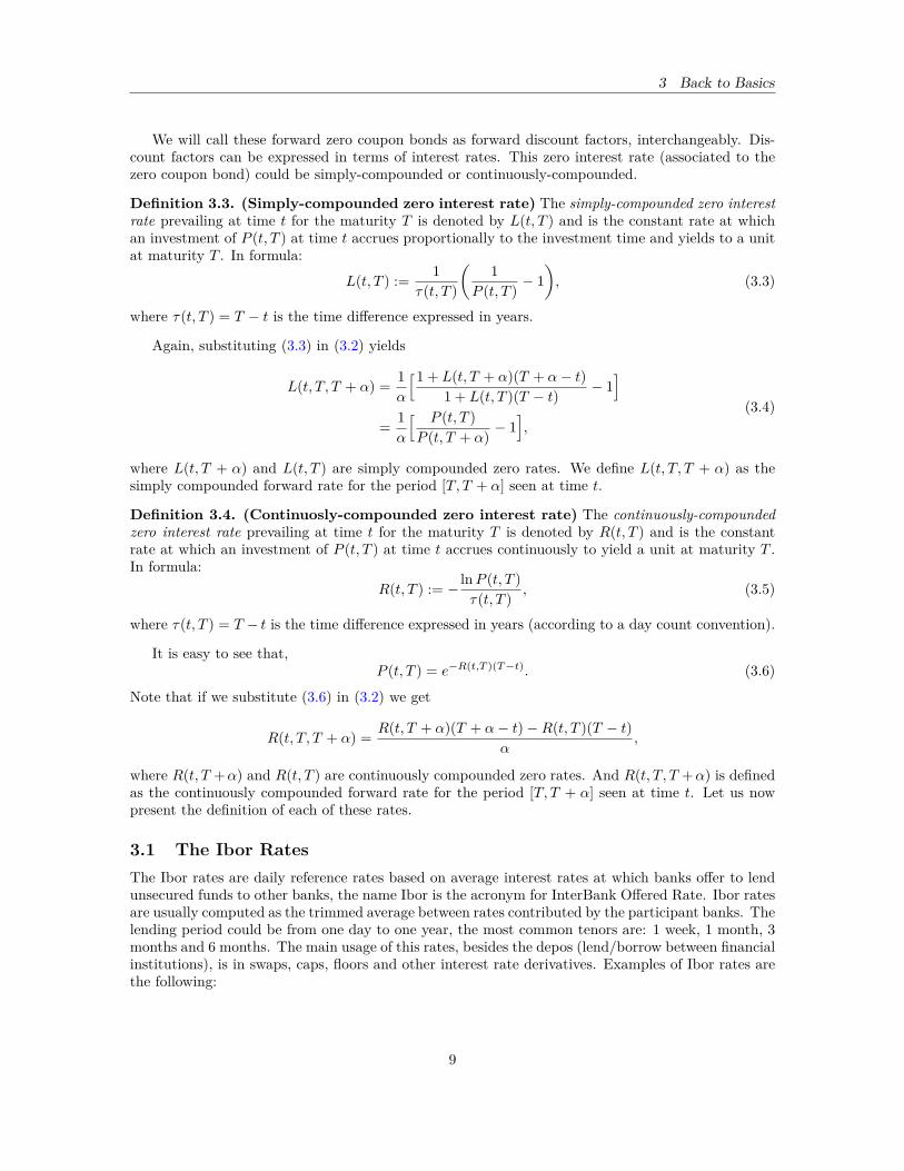
We will call these forward zero coupon bonds as forward discount factors, interchangeably. Dis-count factors can be expressed in terms of interest rates. This zero interest rate (associated to thezero coupon bond) could be simply-compounded or continuously-compounded.
Definition 3.3. (Simply-compounded zero interest rate) The simply-compounded zero interestrate prevailing at time t for the maturity T is denoted by L(t, T ) and is the constant rate at whichan investment of P (t, T ) at time t accrues proportionally to the investment time and yields to a unitat maturity T . In formula:
L(t, T ) := 1τ(t, T )
(1
P (t, T ) − 1), (3.3)
where τ(t, T ) = T − t is the time difference expressed in years.
Again, substituting (3.3) in (3.2) yields
L(t, T, T + α) = 1α
[1 + L(t, T + α)(T + α− t)1 + L(t, T )(T − t) − 1
]= 1α
[ P (t, T )P (t, T + α) − 1
],
(3.4)
where L(t, T + α) and L(t, T ) are simply compounded zero rates. We define L(t, T, T + α) as thesimply compounded forward rate for the period [T, T + α] seen at time t.
Definition 3.4. (Continuosly-compounded zero interest rate) The continuously-compoundedzero interest rate prevailing at time t for the maturity T is denoted by R(t, T ) and is the constantrate at which an investment of P (t, T ) at time t accrues continuously to yield a unit at maturity T .In formula:
R(t, T ) := − lnP (t, T )τ(t, T ) , (3.5)
where τ(t, T ) = T − t is the time difference expressed in years (according to a day count convention).
It is easy to see that,P (t, T ) = e−R(t,T )(T−t). (3.6)
Note that if we substitute (3.6) in (3.2) we get
R(t, T, T + α) = R(t, T + α)(T + α− t)−R(t, T )(T − t)α
,
where R(t, T +α) and R(t, T ) are continuously compounded zero rates. And R(t, T, T +α) is definedas the continuously compounded forward rate for the period [T, T + α] seen at time t. Let us nowpresent the definition of each of these rates.
3.1 The Ibor RatesThe Ibor rates are daily reference rates based on average interest rates at which banks offer to lendunsecured funds to other banks, the name Ibor is the acronym for InterBank Offered Rate. Ibor ratesare usually computed as the trimmed average between rates contributed by the participant banks. Thelending period could be from one day to one year, the most common tenors are: 1 week, 1 month, 3months and 6 months. The main usage of this rates, besides the depos (lend/borrow between financialinstitutions), is in swaps, caps, floors and other interest rate derivatives. Examples of Ibor rates arethe following:
9
3 Back to Basics
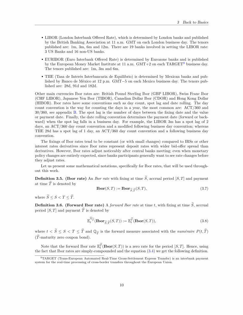
LIBOR (London Interbank Offered Rate), which is determined by London banks and publishedby the British Banking Association at 11 a.m. GMT on each London business day. The tenorspublished are: 1m, 3m, 6m and 12m. There are 19 banks involved in setting the LIBOR rate:3 US Banks and 16 non-US banks.
EURIBOR (Euro Interbank Offered Rate) is determined by Eurozone banks and is publishedby the European Money Market Institute at 11 a.m. GMT+2 on each TARGET9 business day.The tenors published are: 1m, 3m and 6m.
TIIE (Tasa de Interés Interbancaria de Equilibrio) is determined by Mexican banks and pub-lished by Banco de México at 12 p.m. GMT−5 on each Mexico business day. The tenors pub-lished are: 28d, 91d and 182d.
Other main currencies Ibor rates are: British Pound Sterling Ibor (GBP LIBOR), Swiss Franc Ibor(CHF LIBOR), Japanese Yen Ibor (TIBOR), Canadian Dollar Ibor (CDOR) and Hong Kong Dollar(HIBOR). Ibor rates have some conventions such as day count, spot lag and date rolling. The daycount convention is the way for counting the days in a year, the most common are: ACT/360 and30/360, see appendix B. The spot lag is the number of days between the fixing date and the valueor payment date. Finally, the date rolling convention determines the payment date (forward or back-ward) when the spot lag falls in a business day. For example, the LIBOR 3m has a spot lag of 2days, an ACT/360 day count convention and a modified following business day convention; whereasTIIE 28d has a spot lag of 1 day, an ACT/360 day count convention and a following business dayconvention.
The fixings of Ibor rates tend to be constant (or with small changes) compared to IRSs or otherinterest rates derivatives since Ibor rates represent deposit rates with wider bid-offer spread thanderivatives. However, Ibor rates adjust noticeably after central banks meeting; even when monetarypolicy changes are entirely expected, since banks participants generally want to see rate changes beforethey adjust rates.
Let us present some mathematical notations, specifically for Ibor rates, that will be used through-out this work.
Definition 3.5. (Ibor rate) An Ibor rate with fixing at time S, accrual period [S, T ] and paymentat time T is denoted by
Ibor(S, T ) := IborS,T
(S, T ), (3.7)
where S ≤ S < T ≤ T .
Definition 3.6. (Forward Ibor rate) A forward Ibor rate at time t, with fixing at time S, accrualperiod [S, T ] and payment T is denoted by
EQT
t (IborS,T
(S, T )) := ETt (Ibor(S, T )), (3.8)
where t < S ≤ S < T ≤ T and QT
is the forward measure associated with the numéraire P (t, T )(T -maturity zero coupon bond).
Note that the forward Ibor rate ETt (Ibor(S, T )) is a zero rate for the period [S, T ]. Hence, usingthe fact that Ibor rates are simply-compounded and the equation (3.4) we get the following definition.
9TARGET (Trans-European Automated Real-Time Gross-Settlement Express Transfer) is an interbank paymentsystem for the real-time processing of cross-border transfers throughout the European Union.
10
3 Back to Basics
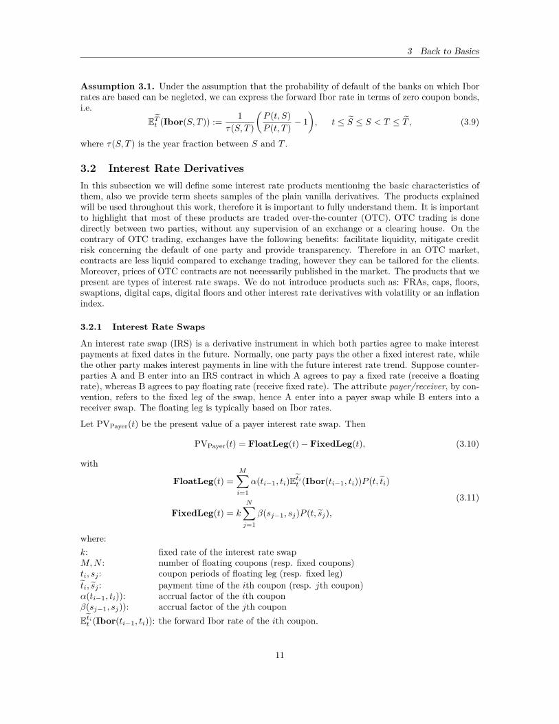
Assumption 3.1. Under the assumption that the probability of default of the banks on which Iborrates are based can be negleted, we can express the forward Ibor rate in terms of zero coupon bonds,i.e.
ETt (Ibor(S, T )) := 1τ(S, T )
(P (t, S)P (t, T ) − 1
), t ≤ S ≤ S < T ≤ T , (3.9)
where τ(S, T ) is the year fraction between S and T .
3.2 Interest Rate DerivativesIn this subsection we will define some interest rate products mentioning the basic characteristics ofthem, also we provide term sheets samples of the plain vanilla derivatives. The products explainedwill be used throughout this work, therefore it is important to fully understand them. It is importantto highlight that most of these products are traded over-the-counter (OTC). OTC trading is donedirectly between two parties, without any supervision of an exchange or a clearing house. On thecontrary of OTC trading, exchanges have the following benefits: facilitate liquidity, mitigate creditrisk concerning the default of one party and provide transparency. Therefore in an OTC market,contracts are less liquid compared to exchange trading, however they can be tailored for the clients.Moreover, prices of OTC contracts are not necessarily published in the market. The products that wepresent are types of interest rate swaps. We do not introduce products such as: FRAs, caps, floors,swaptions, digital caps, digital floors and other interest rate derivatives with volatility or an inflationindex.
3.2.1 Interest Rate Swaps
An interest rate swap (IRS) is a derivative instrument in which both parties agree to make interestpayments at fixed dates in the future. Normally, one party pays the other a fixed interest rate, whilethe other party makes interest payments in line with the future interest rate trend. Suppose counter-parties A and B enter into an IRS contract in which A agrees to pay a fixed rate (receive a floatingrate), whereas B agrees to pay floating rate (receive fixed rate). The attribute payer/receiver, by con-vention, refers to the fixed leg of the swap, hence A enter into a payer swap while B enters into areceiver swap. The floating leg is typically based on Ibor rates.
Let PVPayer(t) be the present value of a payer interest rate swap. Then
PVPayer(t) = FloatLeg(t)− FixedLeg(t), (3.10)
with
FloatLeg(t) =M∑i=1
α(ti−1, ti)Etit (Ibor(ti−1, ti))P (t, ti)
FixedLeg(t) = k
N∑j=1
β(sj−1, sj)P (t, sj),(3.11)
where:k: fixed rate of the interest rate swapM,N : number of floating coupons (resp. fixed coupons)ti, sj : coupon periods of floating leg (resp. fixed leg)ti, sj : payment time of the ith coupon (resp. jth coupon)α(ti−1, ti)): accrual factor of the ith couponβ(sj−1, sj)): accrual factor of the jth couponEtit (Ibor(ti−1, ti)): the forward Ibor rate of the ith coupon.
11
3 Back to Basics
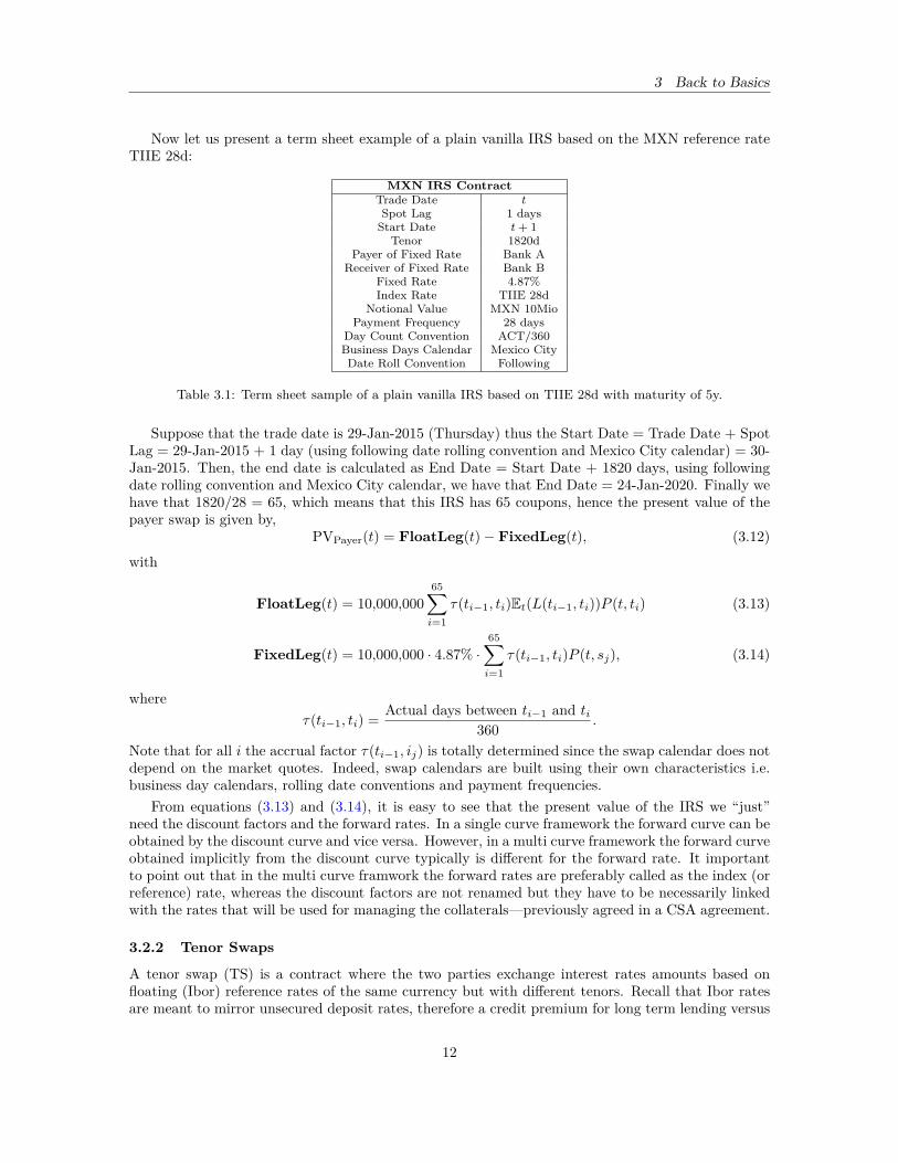
Now let us present a term sheet example of a plain vanilla IRS based on the MXN reference rateTIIE 28d:
MXN IRS ContractTrade Date tSpot Lag 1 daysStart Date t + 1
Tenor 1820dPayer of Fixed Rate Bank A
Receiver of Fixed Rate Bank BFixed Rate 4.87%Index Rate TIIE 28d
Notional Value MXN 10MioPayment Frequency 28 days
Day Count Convention ACT/360Business Days Calendar Mexico CityDate Roll Convention Following
Table 3.1: Term sheet sample of a plain vanilla IRS based on TIIE 28d with maturity of 5y.
Suppose that the trade date is 29-Jan-2015 (Thursday) thus the Start Date = Trade Date + SpotLag = 29-Jan-2015 + 1 day (using following date rolling convention and Mexico City calendar) = 30-Jan-2015. Then, the end date is calculated as End Date = Start Date + 1820 days, using followingdate rolling convention and Mexico City calendar, we have that End Date = 24-Jan-2020. Finally wehave that 1820/28 = 65, which means that this IRS has 65 coupons, hence the present value of thepayer swap is given by,
PVPayer(t) = FloatLeg(t)− FixedLeg(t), (3.12)
with
FloatLeg(t) = 10,000,00065∑i=1
τ(ti−1, ti)Et(L(ti−1, ti))P (t, ti) (3.13)
FixedLeg(t) = 10,000,000 · 4.87% ·65∑i=1
τ(ti−1, ti)P (t, sj), (3.14)
whereτ(ti−1, ti) = Actual days between ti−1 and ti
360 .
Note that for all i the accrual factor τ(ti−1, ij) is totally determined since the swap calendar does notdepend on the market quotes. Indeed, swap calendars are built using their own characteristics i.e.business day calendars, rolling date conventions and payment frequencies.
From equations (3.13) and (3.14), it is easy to see that the present value of the IRS we “just”need the discount factors and the forward rates. In a single curve framework the forward curve can beobtained by the discount curve and vice versa. However, in a multi curve framework the forward curveobtained implicitly from the discount curve typically is different for the forward rate. It importantto point out that in the multi curve framwork the forward rates are preferably called as the index (orreference) rate, whereas the discount factors are not renamed but they have to be necessarily linkedwith the rates that will be used for managing the collaterals—previously agreed in a CSA agreement.
3.2.2 Tenor Swaps
A tenor swap (TS) is a contract where the two parties exchange interest rates amounts based onfloating (Ibor) reference rates of the same currency but with different tenors. Recall that Ibor ratesare meant to mirror unsecured deposit rates, therefore a credit premium for long term lending versus
12
3 Back to Basics
shorter terms has to be payed. This premium is directly included on the spread or basis that is addedon one of the TS legs. The general convention is to add the tenor basis spread to the leg with theshorter tenor [Fujii et al., 2011], while the payment frequency is determined by the longer tenor leg.For example, in the case of the USD market, one party agrees to pay LIBOR 3m quarterly and receiveLIBOR 1m plus the tenor spread; in the latter leg we have to accumulate the monthly payments withcompound interest and settle quarterly to match the 3m tenor leg.
Remark 3.1. In EUR currency market, the tenor swaps are conventionally quoted as two swaps.Hence a quote for paying EURIBOR 3m + 12bps versus receiving EURIBOR 6m has the followingmeaning. In the first swap you pay EURIBOR 3m versus receive a fixed rate (in an annual base). Inthe second swap you pay the same fixed rate plus the spread of 12bps (in an annual base) and receiveEURIBOR 6m [Henrard, 2014]. Note that in this convention the tenor spread is paid on an annualbasis, whereas in USD market the tenor spread is paid quarterly.
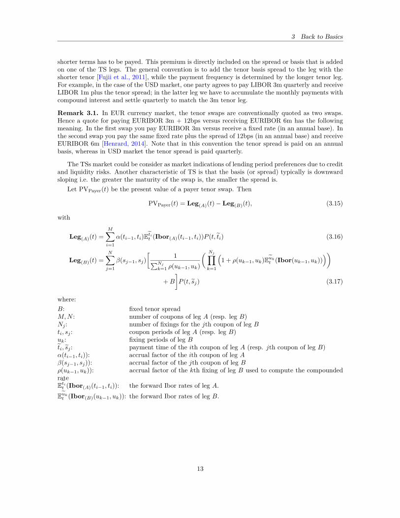
The TSs market could be consider as market indications of lending period preferences due to creditand liquidity risks. Another characteristic of TS is that the basis (or spread) typically is downwardsloping i.e. the greater the maturity of the swap is, the smaller the spread is.
Let PVPayer(t) be the present value of a payer tenor swap. Then
PVPayer(t) = Leg(A)(t)− Leg(B)(t), (3.15)
with
Leg(A)(t) =M∑i=1
α(ti−1, ti)Etit (Ibor(A)(ti−1, ti))P (t, ti) (3.16)
Leg(B)(t) =N∑j=1
β(sj−1, sj)[
1∑Njk=1 ρ(uk−1, uk)
( Nj∏k=1
(1 + ρ(uk−1, uk)Eukt (Ibor(uk−1, uk))
))
+B
]P (t, sj) (3.17)
where:B: fixed tenor spreadM,N : number of coupons of leg A (resp. leg B)Nj : number of fixings for the jth coupon of leg Bti, sj : coupon periods of leg A (resp. leg B)uk: fixing periods of leg Bti, sj : payment time of the ith coupon of leg A (resp. jth coupon of leg B)α(ti−1, ti)): accrual factor of the ith coupon of leg Aβ(sj−1, sj)): accrual factor of the jth coupon of leg Bρ(uk−1, uk)): accrual factor of the kth fixing of leg B used to compute the compoundedrateEtit (Ibor(A)(ti−1, ti)): the forward Ibor rates of leg A.Eukt (Ibor(B)(uk−1, uk)): the forward Ibor rates of leg B.
13
3 Back to Basics
LIBOR 3m vs 1m 5y ContractTrade Date tSpot Lag 2 daysStart Date t + 2
Tenor 5ySpread (Leg) +0.10% (LIBOR 1m)Index Rates LIBOR 1m & LIBOR 3m
Notional Value USD 10MioPayment Frequency 3 Months
Day Count Convention ACT/360Business Days Calendar New York & LondonDate Roll Convention Modified Following
Table 3.2: Example of a plain vanilla 5y tenor swap contract.
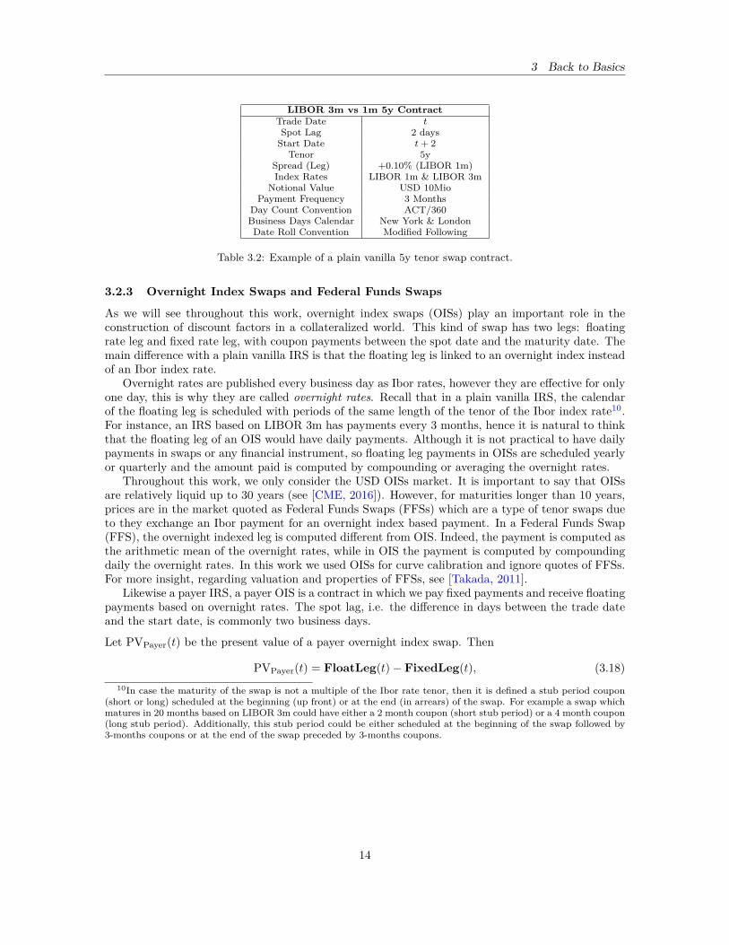
3.2.3 Overnight Index Swaps and Federal Funds Swaps
As we will see throughout this work, overnight index swaps (OISs) play an important role in theconstruction of discount factors in a collateralized world. This kind of swap has two legs: floatingrate leg and fixed rate leg, with coupon payments between the spot date and the maturity date. Themain difference with a plain vanilla IRS is that the floating leg is linked to an overnight index insteadof an Ibor index rate.
Overnight rates are published every business day as Ibor rates, however they are effective for onlyone day, this is why they are called overnight rates. Recall that in a plain vanilla IRS, the calendarof the floating leg is scheduled with periods of the same length of the tenor of the Ibor index rate10.For instance, an IRS based on LIBOR 3m has payments every 3 months, hence it is natural to thinkthat the floating leg of an OIS would have daily payments. Although it is not practical to have dailypayments in swaps or any financial instrument, so floating leg payments in OISs are scheduled yearlyor quarterly and the amount paid is computed by compounding or averaging the overnight rates.
Throughout this work, we only consider the USD OISs market. It is important to say that OISsare relatively liquid up to 30 years (see [CME, 2016]). However, for maturities longer than 10 years,prices are in the market quoted as Federal Funds Swaps (FFSs) which are a type of tenor swaps dueto they exchange an Ibor payment for an overnight index based payment. In a Federal Funds Swap(FFS), the overnight indexed leg is computed different from OIS. Indeed, the payment is computed asthe arithmetic mean of the overnight rates, while in OIS the payment is computed by compoundingdaily the overnight rates. In this work we used OISs for curve calibration and ignore quotes of FFSs.For more insight, regarding valuation and properties of FFSs, see [Takada, 2011].
Likewise a payer IRS, a payer OIS is a contract in which we pay fixed payments and receive floatingpayments based on overnight rates. The spot lag, i.e. the difference in days between the trade dateand the start date, is commonly two business days.
Let PVPayer(t) be the present value of a payer overnight index swap. Then
PVPayer(t) = FloatLeg(t)− FixedLeg(t), (3.18)10In case the maturity of the swap is not a multiple of the Ibor rate tenor, then it is defined a stub period coupon
(short or long) scheduled at the beginning (up front) or at the end (in arrears) of the swap. For example a swap whichmatures in 20 months based on LIBOR 3m could have either a 2 month coupon (short stub period) or a 4 month coupon(long stub period). Additionally, this stub period could be either scheduled at the beginning of the swap followed by3-months coupons or at the end of the swap preceded by 3-months coupons.
14
3 Back to Basics
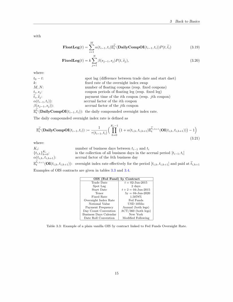
with
FloatLeg(t) =M∑i=1
α(ti−1, ti)Etit (DailyCompOI(ti−1, ti))P (t, ti) (3.19)
FixedLeg(t) = k
N∑j=1
β(sj−1, sj)P (t, sj), (3.20)
where:t0 − t: spot lag (difference between trade date and start daet)k: fixed rate of the overnight index swapM,N : number of floating coupons (resp. fixed coupons)ti, sj : coupon periods of floating leg (resp. fixed leg)ti, sj : payment time of the ith coupon (resp. jth coupon)α(ti−1, ti)): accrual factor of the ith couponβ(sj−1, sj)): accrual factor of the jth couponEtit (DailyCompOI(ti−1, ti)): the daily compounded overnight index rate.
The daily compounded overnight index rate is defined as
Etit (DailyCompOI(ti−1, ti)) := 1τ(ti−1, ti)
(Ki−1∏h=0
(1 + α(ti,h, ti,h+1)Eti,h+1
t (OI(ti,h, ti,h+1)))− 1)
(3.21)where:Ki: number of business days between ti−1 and titi,hKih=0: is the collection of all business days in the accrual period [ti−1, ti]α(ti,h, ti,h+1): accrual factor of the hth business dayEti,h+1t (OI(ti,h, ti,h+1)): overnight index rate effectively for the period [ti,h, ti,h+1] and paid at ti,h+1
Examples of OIS contracts are given in tables 3.3 and 3.4.
OIS (Fed Fund) 5y ContractTrade Date t = 02-Jun-2015Spot Lag 2 daysStart Date t + 2 = 04-Jun-2015
Tenor 5y = 04-Jun-2020Fixed Rate 1.5078%
Overnight Index Rate Fed FundsNotional Value USD 10Mio
Payment Frequency Annual (both legs)Day Count Convention ACT/360 (both legs)Business Days Calendar New YorkDate Roll Convention Modified Following
Table 3.3: Example of a plain vanilla OIS 5y contract linked to Fed Funds Overnight Rate.
15
3 Back to Basics
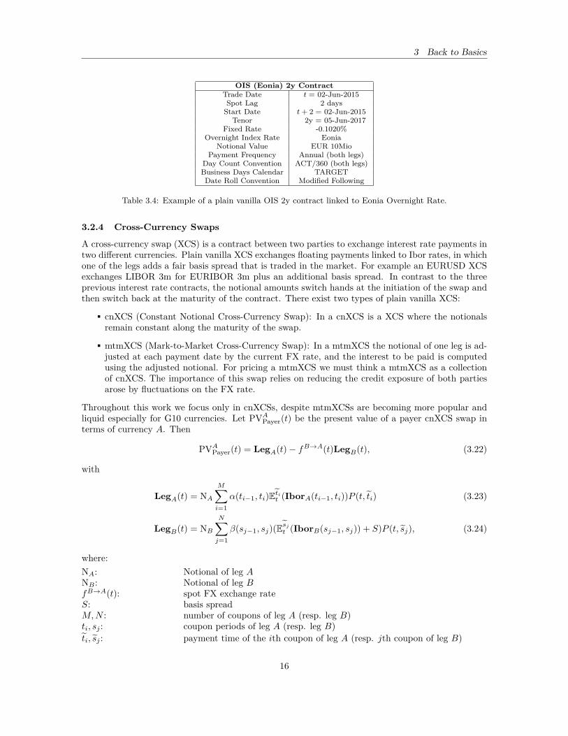
OIS (Eonia) 2y ContractTrade Date t = 02-Jun-2015Spot Lag 2 daysStart Date t + 2 = 02-Jun-2015
Tenor 2y = 05-Jun-2017Fixed Rate -0.1020%
Overnight Index Rate EoniaNotional Value EUR 10Mio
Payment Frequency Annual (both legs)Day Count Convention ACT/360 (both legs)Business Days Calendar TARGETDate Roll Convention Modified Following
Table 3.4: Example of a plain vanilla OIS 2y contract linked to Eonia Overnight Rate.
3.2.4 Cross-Currency Swaps
A cross-currency swap (XCS) is a contract between two parties to exchange interest rate payments intwo different currencies. Plain vanilla XCS exchanges floating payments linked to Ibor rates, in whichone of the legs adds a fair basis spread that is traded in the market. For example an EURUSD XCSexchanges LIBOR 3m for EURIBOR 3m plus an additional basis spread. In contrast to the threeprevious interest rate contracts, the notional amounts switch hands at the initiation of the swap andthen switch back at the maturity of the contract. There exist two types of plain vanilla XCS:
cnXCS (Constant Notional Cross-Currency Swap): In a cnXCS is a XCS where the notionalsremain constant along the maturity of the swap.
mtmXCS (Mark-to-Market Cross-Currency Swap): In a mtmXCS the notional of one leg is ad-justed at each payment date by the current FX rate, and the interest to be paid is computedusing the adjusted notional. For pricing a mtmXCS we must think a mtmXCS as a collectionof cnXCS. The importance of this swap relies on reducing the credit exposure of both partiesarose by fluctuations on the FX rate.
Throughout this work we focus only in cnXCSs, despite mtmXCSs are becoming more popular andliquid especially for G10 currencies. Let PVAPayer(t) be the present value of a payer cnXCS swap interms of currency A. Then
PVAPayer(t) = LegA(t)− fB→A(t)LegB(t), (3.22)
with
LegA(t) = NAM∑i=1
α(ti−1, ti)Etit (IborA(ti−1, ti))P (t, ti) (3.23)
LegB(t) = NBN∑j=1
β(sj−1, sj)(Esjt (IborB(sj−1, sj)) + S)P (t, sj), (3.24)
where:NA: Notional of leg ANB : Notional of leg BfB→A(t): spot FX exchange rateS: basis spreadM,N : number of coupons of leg A (resp. leg B)ti, sj : coupon periods of leg A (resp. leg B)ti, sj : payment time of the ith coupon of leg A (resp. jth coupon of leg B)
16
3 Back to Basics
α(ti−1, ti)): accrual factor of the ith coupon of leg Aβ(sj−1, sj)): accrual factor of the jth coupon of leg BEtit (Ibor(A)(ti−1, ti)): the forward Ibor rate of leg A.Esjt (Ibor(B)(sj−1, sj)): the forward Ibor rate of leg B.
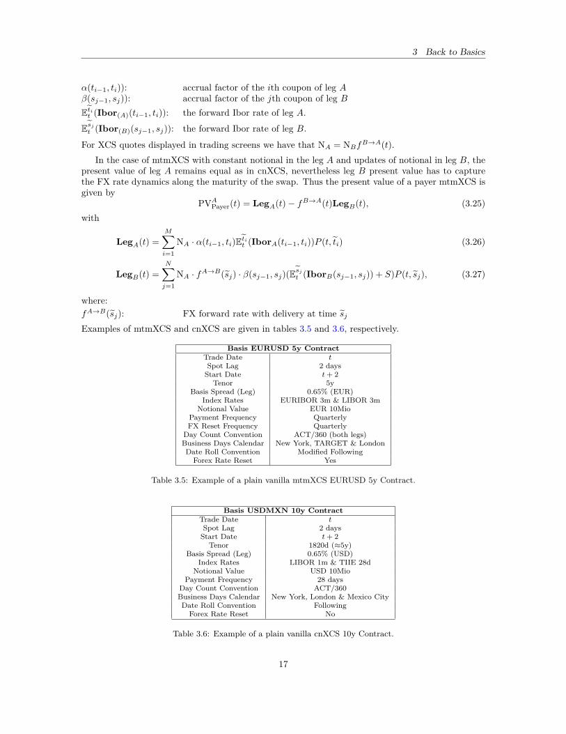
For XCS quotes displayed in trading screens we have that NA = NBfB→A(t).In the case of mtmXCS with constant notional in the leg A and updates of notional in leg B, the
present value of leg A remains equal as in cnXCS, nevertheless leg B present value has to capturethe FX rate dynamics along the maturity of the swap. Thus the present value of a payer mtmXCS isgiven by
PVAPayer(t) = LegA(t)− fB→A(t)LegB(t), (3.25)with
LegA(t) =M∑i=1
NA · α(ti−1, ti)Etit (IborA(ti−1, ti))P (t, ti) (3.26)
LegB(t) =N∑j=1
NA · fA→B(sj) · β(sj−1, sj)(Esjt (IborB(sj−1, sj)) + S)P (t, sj), (3.27)
where:fA→B(sj): FX forward rate with delivery at time sjExamples of mtmXCS and cnXCS are given in tables 3.5 and 3.6, respectively.
Basis EURUSD 5y ContractTrade Date tSpot Lag 2 daysStart Date t + 2
Tenor 5yBasis Spread (Leg) 0.65% (EUR)
Index Rates EURIBOR 3m & LIBOR 3mNotional Value EUR 10Mio
Payment Frequency QuarterlyFX Reset Frequency Quarterly
Day Count Convention ACT/360 (both legs)Business Days Calendar New York, TARGET & LondonDate Roll Convention Modified FollowingForex Rate Reset Yes
Table 3.5: Example of a plain vanilla mtmXCS EURUSD 5y Contract.
Basis USDMXN 10y ContractTrade Date tSpot Lag 2 daysStart Date t + 2
Tenor 1820d (≈5y)Basis Spread (Leg) 0.65% (USD)
Index Rates LIBOR 1m & TIIE 28dNotional Value USD 10Mio
Payment Frequency 28 daysDay Count Convention ACT/360Business Days Calendar New York, London & Mexico CityDate Roll Convention FollowingForex Rate Reset No
Table 3.6: Example of a plain vanilla cnXCS 10y Contract.
17
4 Pricing IRS in Single-curve Framework
4 Pricing IRS in Single-curve FrameworkIn this section we present the formulas for pricing an interest rate swap in a single-curve framework,specifically in the MXN currency market. This framework is important from a historical point of viewsince they explain and serve as a basis of the multi-curve framework. The general idea of the single-curve framework is that all interest rate derivative, in the same currency, depend on only one curve,which is supposed to be the discount curve and Ibor index curve.
4.1 Case of MXNThis section presents the construction the MXN yield curve under the assumption that the plainvanilla swaps traded on the market do not have a collateral agreement. Therefore, we are assumingthat the TIIE 28d rate (mexican interbank offered rate) is risk-free and illiquidity or credit issues ofparticipant banks are neglected, i.e., we do not need to incorporate a collateral rate. This frameworkis known as single-curve framework, since one unique curve is used for extract discount factors andforward rates. Before the financial crisis in 2007, this framework was widely used and was consideredthe correct method for pricing and valuation of interest rate derivatives. It is important to remindthat this model assumes that a financial institution borrows and lends money with the same risk-freerate, in this case TIIE 28d rate.
From equations (3.10) and (3.11), we have that the present value of a payer IRS of TIIE28d is givenby
PV(t) =M∑i=1
α(ti−1, ti)Etit (TIIE28D(ti−1, ti))P (t, ti)− kN∑j=1
β(sj−1, sj)P (t, sj), (4.1)
Since in a plain vanilla IRS linked to TIIE 28d the number of coupons in both legs are the same, theend date of each coupon period equals the payment date i.e. ti = ti for all i, and day count conventionis the same for each leg, then equation (4.1) reduces to
PV(t) =N∑i=1
α(ti−1, ti)Etit (TIIE28D(ti−1, ti))P (t, ti)− kN∑i=1
α(ti−1, ti)P (t, ti), (4.2)
where:k: fixed rate of the plain vanilla interest rate swapN : number of couponsti: coupon periods (start date, end date and payment date)α(ti−1, ti)): accrual factor of the ith couponEtit (TIIE28D(ti−1, ti)): the forward TIIE 28d rate of the ith coupon.
Now, in a single-curve framework we have that
Etit (TIIE28D(ti−1, ti)) =(
1τ(ti−1, ti)
(P (t, ti−1)P (t, ti)
− 1))
. (4.3)
Note that in equation (4.3) we use τ as day count factor instead of α that is used in the swap. Itis important to point out that, in general, α(ti−1, ti)) 6= τ(ti−1, ti)), this is because α(ti−1, ti)) isthe accrual factor (year fraction) used for the payment of the ith coupon, whereas τ(ti−1, ti)) is theday count (year fraction) used for the interpolation and construction of zero curve. In the swapsmarket, the accrual factors of payments usually are based on an ACT/360 or 30/360 convention, whileinterpolation methods for the construction of zero curves typically used an ACT/ACT or ACT/365convention.
18
4 Pricing IRS in Single-curve Framework
Tenor Rate(%) Type
Number ofUnknownVariables
Unknown Variables
ON 3.0500 Cash 1 P (t, t+ 1)TN 3.0500 Cash 1 P (t, t+ 2)
28D 3.2950 Cash 1 P (t, T28D)84D 3.3200 Swap 3 P (t, t+ 1), P (t, T28D), . . . , P (t, T84D)
168D 3.4300 Swap 6 P (t, t+ 1), P (t, T28D), . . . , P (t, T168D)252D 3.5620 Swap 9 P (t, t+ 1), P (t, T28D), . . . , P (t, T252D)364D 3.7350 Swap 13 P (t, t+ 1), P (t, T28D), . . . , P (t, T364D)728D 4.2360 Swap 26 P (t, t+ 1), P (t, T28D), . . . , P (t, T728D)
1092D 4.6710 Swap 39 P (t, t+ 1), P (t, T28D), . . . , P (t, T1092D)1456D 5.0510 Swap 52 P (t, t+ 1), P (t, T28D), . . . , P (t, T1456D)1820D 5.3610 Swap 65 P (t, t+ 1), P (t, T28D), . . . , P (t, T1820D)2548D 5.8630 Swap 91 P (t, t+ 1), P (t, T28D), . . . , P (t, T2548D)3640D 6.2380 Swap 130 P (t, t+ 1), P (t, T28D), . . . , P (t, T3640D)4368D 6.4280 Swap 156 P (t, t+ 1), P (t, T28D), . . . , P (t, T4368D)5460D 6.6320 Swap 195 P (t, t+ 1), P (t, T28D), . . . , P (t, T5260D)7280D 6.8310 Swap 260 P (t, t+ 1), P (t, T28D), . . . , P (t, T7280D)
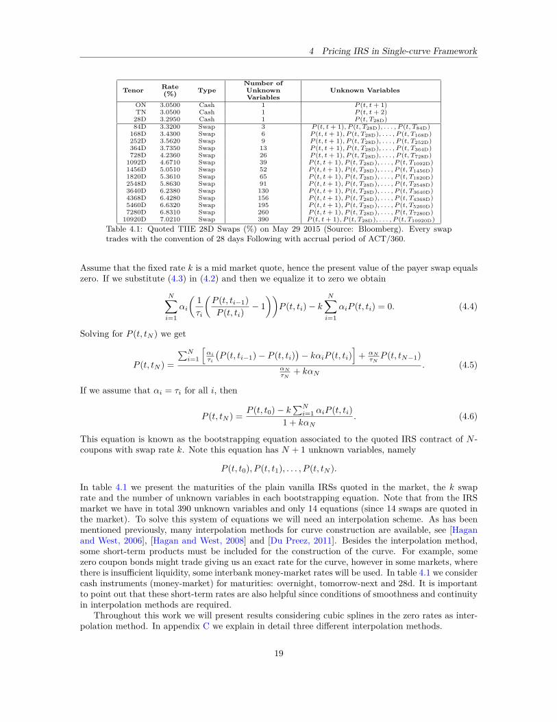
10920D 7.0210 Swap 390 P (t, t+ 1), P (t, T28D), . . . , P (t, T10920D)Table 4.1: Quoted TIIE 28D Swaps (%) on May 29 2015 (Source: Bloomberg). Every swaptrades with the convention of 28 days Following with accrual period of ACT/360.
Assume that the fixed rate k is a mid market quote, hence the present value of the payer swap equalszero. If we substitute (4.3) in (4.2) and then we equalize it to zero we obtain
N∑i=1
αi
(1τi
(P (t, ti−1)P (t, ti)
− 1))
P (t, ti)− kN∑i=1
αiP (t, ti) = 0. (4.4)
Solving for P (t, tN ) we get
P (t, tN ) =
∑Ni=1
[αiτi
(P (t, ti−1)− P (t, ti)
)− kαiP (t, ti)
]+ αN
τNP (t, tN−1)
αNτN
+ kαN. (4.5)
If we assume that αi = τi for all i, then
P (t, tN ) =P (t, t0)− k
∑Ni=1 αiP (t, ti)
1 + kαN. (4.6)
This equation is known as the bootstrapping equation associated to the quoted IRS contract of N -coupons with swap rate k. Note this equation has N + 1 unknown variables, namely
P (t, t0), P (t, t1), . . . , P (t, tN ).
In table 4.1 we present the maturities of the plain vanilla IRSs quoted in the market, the k swaprate and the number of unknown variables in each bootstrapping equation. Note that from the IRSmarket we have in total 390 unknown variables and only 14 equations (since 14 swaps are quoted inthe market). To solve this system of equations we will need an interpolation scheme. As has beenmentioned previously, many interpolation methods for curve construction are available, see [Haganand West, 2006], [Hagan and West, 2008] and [Du Preez, 2011]. Besides the interpolation method,some short-term products must be included for the construction of the curve. For example, somezero coupon bonds might trade giving us an exact rate for the curve, however in some markets, wherethere is insufficient liquidity, some interbank money-market rates will be used. In table 4.1 we considercash instruments (money-market) for maturities: overnight, tomorrow-next and 28d. It is importantto point out that these short-term rates are also helpful since conditions of smoothness and continuityin interpolation methods are required.
Throughout this work we will present results considering cubic splines in the zero rates as inter-polation method. In appendix C we explain in detail three different interpolation methods.
19
4 Pricing IRS in Single-curve Framework
Note that the bootstrapping equation (4.6) is expressed in terms of discount factors, however thisequation can be expressed in term of zero rates
R(t, tN ) = − 1τN
ln[P (t, t0)− k
∑Ni=1 αiP (t, ti)
1 + kαN
]= 1τN
ln[
1 + kαN
e−τt0R(t,t0) − k∑Ni=1 αie
−τtiR(t,ti)
].
(4.7)
Hence the system of equations of table 4.1 is given byR(t, tNl) = 1τNl
ln[
1 + kαNl
e−τt0R(t,t0) − k∑Nli=1 αie
−τtiR(t,ti)
]l = 1, 2, . . . , 14 (swaps)
R(t, t0) = RON, R(t0, t0 + 1D) = RTN, R(t0, t0 + 28D) = R28D. (cash)(4.8)
With this equation we proceed to the bootstrapping algorithm which relies on an iterative solutionalgorithm. The idea is the following:
1. Take the rates R(t, x) already known from the money market
2. Guess initial values for R(t, tN ) where tN are the maturities of the 14th swaps
3. With the interpolation method we calculate R(t, ti) for all ith coupon date
4. Insert these rates into the right-hand side of equation (4.7) and solve for R(t, tN )
5. We take these new guesses and again apply the interpolation algorithm
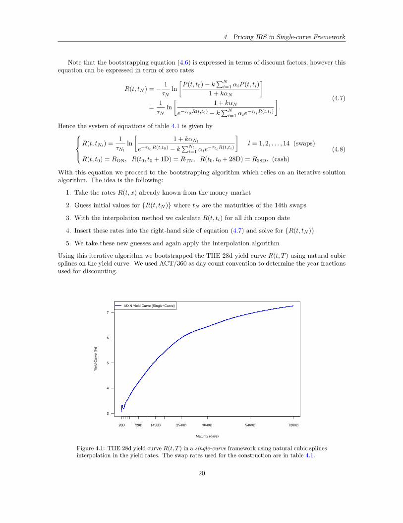
Using this iterative algorithm we bootstrapped the TIIE 28d yield curve R(t, T ) using natural cubicsplines on the yield curve. We used ACT/360 as day count convention to determine the year fractionsused for discounting.
3
4
5
6
7
Maturity (days)
Yie
ld C
urve
(%
)
28D 728D 1456D 2548D 3640D 5460D 7280D
MXN Yield Curve (Single−Curve)
Figure 4.1: TIIE 28d yield curve R(t, T ) in a single-curve framework using natural cubic splinesinterpolation in the yield rates. The swap rates used for the construction are in table 4.1.
20
4 Pricing IRS in Single-curve Framework
0.2
0.4
0.6
0.8
1.0
Maturity (days)
Dis
coun
t Fac
tor
28D 728D 1456D 2548D 3640D 5460D 7280D
MXN Discount Curve (Single−Curve)
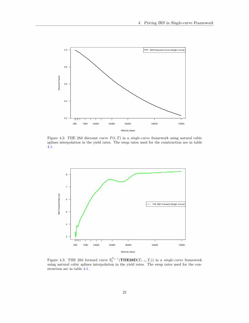
Figure 4.2: TIIE 28d discount curve P (t, T ) in a single-curve framework using natural cubicsplines interpolation in the yield rates. The swap rates used for the construction are in table4.1.
3
4
5
6
7
8
Maturity (days)
28D
For
war
d R
ate
(%)
28D 728D 1456D 2548D 3640D 5460D 7280D
TIIE 28D−Forward (Single−Curve)
Figure 4.3: TIIE 28d forward curve ETi−1t (TIIE28D(Ti−1, Ti)) in a single-curve framework
using natural cubic splines interpolation in the yield rates. The swap rates used for the con-struction are in table 4.1.
21
5 Pricing IRS in a Multi-curve Framework (in Presence of Collateral)
5 Pricing IRS in a Multi-curve Framework (in Presence ofCollateral)
In this section we present the valuation frameworks for pricing interest rate swaps (IRSs) in a multi-curve framework with a collateral account associated to the derivative. The section is divided inthree main subsections. In the first subsection we establish the general collateral framework, i.e. weexplain how a a collateral account works, which are the advantages and disadvantages for having acollateral framework and what assumptions do we have to make for pricing collateralized IRSs. Inthe second subsection we focus on the easiest case: when the currency of payoffs of the derivativeand the collateral currency coincide. Indeed we present the curve calibration of IRSs and OISs inUSD currency. In the third and last subsection we give the multiple currencies collateral framework,i.e. when the payoffs’ currency is different of the collateral currency. Furthermore we exemplify thedifferences between EUR and MXN pricing of IRSs when the collateral currency is USD. The materialand results presented in this section were mostly taken from [Fujii et al., 2010b], [Fujii et al., 2010a],[Fujii et al., 2011], [Piterbarg, 2010], [Piterbarg, 2012] and [Green, 2015].
5.1 Pricing of Collateralized ProductsAs we saw in the introduction there have been a lot of changes in the market since the financialturmoil in 2008. One of the most important questions that has to be answered since then is: whatis the risk-free rate? Before we try to answer this question let us present a quote taken from [Green,2015].
Nothing in life and nothing that we do is risk-free
Ken Salazar, US Politician
We have already seen that LIBOR rates in the USD market are not a good proxy anymore after theLehman Brothers default. Recall that the world has entered into a new phase in which high-creditrating banks are able to default in matter of weeks. Once we accepted that LIBOR rate is not a goodchoice of risk-free rate, it is normal to think on yield rates of government bonds. However governmentsalso default, as the case of Greece in the Eurozone or Argentina in Latin America. Another alternativefor risk-free rate might be the repo rate. The repo rate is an interest rate that is paid on a collateralizedloan and therefore should be very close to being risk-free, unfortunately the repo market is only liquidfor maturities up to one year, for our purpose for the valuation of long-term IRS we need a marketwith long-dated maturities. Hence the best candidate for this purpose is the OIS market. There aremany valid reasons for using overnight rates as risk-free rates, let us present some of these reasons:
1. Overnight Rates such as Fed Funds and Eonia are based on actual trades, indeed these ratesare calculated by the average rate at which these transactions occur
2. The OIS market is active and liquid in several currencies and have maturities of up to 30 years.3. Lending and borrowing money in this market has a low counterparty credit risk since transac-
tions occur in a daily basis so the counterparty might change also daily4. ISDA contracts typically used this rates as the cash collateral rate
So now we know that overnight rates are widely used as collateral rates. In this section we will provethat the collateral rate in the presence of a perfect CSA is the curve used for discounting. But beforewe proof this fact let us explain briefly how does the collateral works and why it is important in thevaluation of interest rate derivatives.
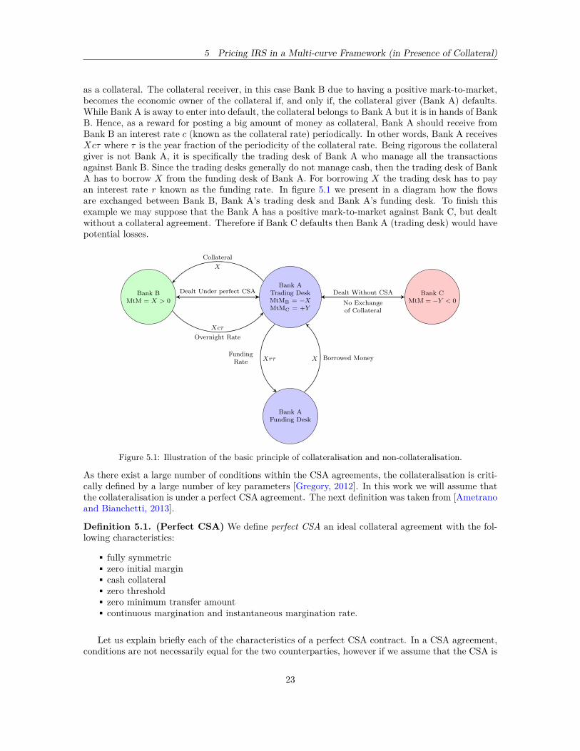
Suppose that a Bank B has a big and positive exposure X (sum of all derivatives transactions) againstBank A. There is clearly a strong risk for the Bank B if the Bank A is to default. With a collateralagreement Bank B limits this exposure since Bank A has to post this mark-to-market (exposure) X
22
5 Pricing IRS in a Multi-curve Framework (in Presence of Collateral)
as a collateral. The collateral receiver, in this case Bank B due to having a positive mark-to-market,becomes the economic owner of the collateral if, and only if, the collateral giver (Bank A) defaults.While Bank A is away to enter into default, the collateral belongs to Bank A but it is in hands of BankB. Hence, as a reward for posting a big amount of money as collateral, Bank A should receive fromBank B an interest rate c (known as the collateral rate) periodically. In other words, Bank A receivesXcτ where τ is the year fraction of the periodicity of the collateral rate. Being rigorous the collateralgiver is not Bank A, it is specifically the trading desk of Bank A who manage all the transactionsagainst Bank B. Since the trading desks generally do not manage cash, then the trading desk of BankA has to borrow X from the funding desk of Bank A. For borrowing X the trading desk has to payan interest rate r known as the funding rate. In figure 5.1 we present in a diagram how the flowsare exchanged between Bank B, Bank A’s trading desk and Bank A’s funding desk. To finish thisexample we may suppose that the Bank A has a positive mark-to-market against Bank C, but dealtwithout a collateral agreement. Therefore if Bank C defaults then Bank A (trading desk) would havepotential losses.
Bank ATrading DeskMtMB = −XMtMC = +Y
Bank AFunding Desk
Bank CMtM = −Y < 0
Bank BMtM = X > 0
Dealt Under perfect CSA Dealt Without CSA
No Exchangeof Collateral
Xcτ
Overnight Rate
Collateral
X
Borrowed MoneyXXrτFundingRate
Figure 5.1: Illustration of the basic principle of collateralisation and non-collateralisation.
As there exist a large number of conditions within the CSA agreements, the collateralisation is criti-cally defined by a large number of key parameters [Gregory, 2012]. In this work we will assume thatthe collateralisation is under a perfect CSA agreement. The next definition was taken from [Ametranoand Bianchetti, 2013].
Definition 5.1. (Perfect CSA) We define perfect CSA an ideal collateral agreement with the fol-lowing characteristics:
fully symmetriczero initial margincash collateralzero thresholdzero minimum transfer amountcontinuous margination and instantaneous margination rate.
Let us explain briefly each of the characteristics of a perfect CSA contract. In a CSA agreement,conditions are not necessarily equal for the two counterparties, however if we assume that the CSA is
23
5 Pricing IRS in a Multi-curve Framework (in Presence of Collateral)
fully symmetric hence both parties have the same conditions and indeed both have to post collateral.The initial margin is the amount of money that the counterparties have to post when closing thedeal. A zero initial margin implies that neither of the counterparties have to post an initial margin.The threshold is a level of exposure below which collateral will not be called. The threshold thereforerepresents an amount of undercollateralized exposure. If the exposure is above the threshold, onlythe incremental exposure will be collateralized. In the case of threshold equal to zero then everymovement in mark-to-market should be collateralised. The minimum transfer amount defines theminimum amount of collateral that can be called for at a time. Collateral cannot be transferred inblocks that are smaller than the minimum transfer amount, but with this minimum transfer amountequal to zero then every update of mark-to-market has to be transferred. Finally the marginationfrequency refers to the periodic timescale which may be called and returned. Intraday margination iscommon for plain vanilla products such as repos and for derivatives cleared via central counterparties.For the perfect CSA, the continuous margination assumption is in practice operationally impossible,however this assumption will help us for the mathematical model. In the next subsection, we presentthe valuation framework for pricing any derivative with a given collateral account, this model is usefulonly when the derivative currency coincides with the collateral currency.
5.2 Valuation Framework in a Single CurrencyLet X be a derivative (of some underlying product) with maturity at time T and with (h(t))t≥0 priceprocess. Let V (t) be a stochastic self-financing collateral account under a perfect CSA agreement fora position of derivatives X11. Assume that the derivative payoff and the collateral account are postedin the same currency, later we will present the case of different currencies. Then the stochastic processof the collateral account is given by
dV (s) = α [r(s)− c(s)]V (s)ds+ a(s)dh(s), (5.1)
where, α is the percentage of collateralization on the derivative X, r(s) and c(s) are the fundingrate and the collateral rate at time s, respectively, h(s) is the value of the derivative at time s whichmatures at time T with cash flow h(T ), and a(s) represents the number of positions of the derivative attime s. Equation (5.1) can be interpreted as follows: the change of the value of the collateral accountdepends on the interest differential earned on the partial posted collateral over time as well as thechange in the value of the a(s) underlying derivatives. Note that equation (5.1) has the form dQ(t) =(µ(t)−rf (t))Q(t)dt+σQ(t)dW (t) which is similar to the dynamic for pricing future contracts of stocksin a Black-Scholes setting. To solve (5.1) we have to multiply the equation by exp(
∫ Tsαy(η)dη), where
y(s) = r(s)− c(s), to get
e
∫ Tsαy(η)dη
dV (s) = e
∫ Tsαy(η)dη
αy(s)V (s)ds+ e
∫ Tsαy(η)dη
a(s)dh(s). (5.2)
Integrating (5.2) over [t, T ] give us∫ T
t
e
∫ Tsαy(η)dη
dV (s) =∫ T
t
e
∫ Tsαy(η)dη
αy(s)V (s)ds+∫ T
t
e
∫ Tsαy(η)dη
a(s)dh(s). (5.3)
Let us define u = e
∫ Tsαy(η)dη and dv = dV (s), using integration by parts formula we obtain∫
udv = uv −∫vdu (5.4)∫ T
t
e
∫ Tsαy(η)dη
dV (s) = e
∫ Tsαy(η)dη
V (s)∣∣∣Tt
+∫ T
t
V (s)e∫ Tsαy(η)dη
αy(s)ds. (5.5)
11We will assume the conditions under a perfect CSA (see definition 5.1). Nevertheless the model is built thinkingthe derivative cab be partially collateralised. The idea behind this assumption is to show the difference of valuationbetween collateralised and non-collateralised.
24
5 Pricing IRS in a Multi-curve Framework (in Presence of Collateral)
Then using (5.3) and (5.5) we have
V (T ) = e
∫ Ttαy(η)dη
V (t) +∫ T
t
e
∫ Tsαy(η)dη
a(s)dh(s). (5.6)
As in [Fujii et al., 2010b], we adopt the trading strategy specified byV (t) = h(t)
a(s) = e
∫ stαy(η)dη (5.7)
If we substitute the trading strategy (5.7) in (5.6) we get
V (T ) = e
∫ Ttαy(η)dη
V (t) +∫ T
t
e
∫ Tsαy(η)dη
a(s)dh(s)
= e
∫ Ttαy(η)dη
h(t) +∫ T
t
e
∫ Tsαy(η)dη+
∫ stαy(η)dη
dh(s)
= e
∫ Ttαy(η)dη
h(t) + e
∫ Ttαy(η)dη
∫ T
t
dh(s)
= e
∫ Ttαy(η)dη
h(t) + e
∫ Ttαy(η)dη
h(T )− e∫ Ttαy(η)dη
h(t)
= e
∫ Ttαy(η)dη
h(T ) (5.8)
Now we can calculate the present value h(t) of the derivative X considering the collateral account Vassociated to it. Using the risk-neutral measure Q with numéraire B(T ) = exp(
∫ Ttr(s)ds) (money-
market account) yields
h(t) = B(t)EQt
[V (T )B(T )
]
= EQt
e∫ Tt αy(s)dsh(T )
e
∫ Ttr(s)ds
= EQ
t
[e−∫ Ttr(s)−α(r(s)−c(s))ds
h(T )]
= EQt
[e−∫ Tt
(1−α)r(s)+αc(s)dsh(T )
]. (5.9)
Therefore, if X is fully collateralized, i.e. α = 1, then
h(t) = EQt
[e−∫ Ttc(s)ds
h(T )], (5.10)
which implies that collateralized cash flows must be discounted considering the collateral rate. Unlikethis case, if X is not collateralized, i.e. α = 0, then
h(t) = EQt
[e−∫ Ttr(s)ds
h(T )], (5.11)
which implies that uncollateralized cash flows must be discounted considering the funding rate.Definition 5.2. We denote the price of a T -maturity fully-collateralized zero coupon bond by
P c(t, T ) = EQt
[e−∫ Ttc(s)ds
]. (5.12)
We will use this definition to introduce the forward measure under collateralization.
25
5 Pricing IRS in a Multi-curve Framework (in Presence of Collateral)
5.2.1 Forward Measure
Before we can go on, let us present in an informal way the concept of Radon-Nikodým derivative andtwo important results that are used to build the collateralized forward measure. Consider a generalfinite probability space (Ω,F,P). Suppose that on this space we have another probability measure Q.Let us assume that P > 0 and Q > 0 for every ω ∈ Ω, so we can define
Z(ω) = Q(ω)P(ω) . (5.13)
Since Z > 0 for all ω ∈ Ω and Z is a random variable we can compute the expected value of Z undermeasure P
EP(Z) =∑ω∈Ω
Z(ω)P(ω) =∑ω∈Ω
Q(ω)P(ω) P(ω) =
∑ω∈Ω
Q(ω) = 1. (5.14)
Now for any random variable Y ,
EP(ZY ) =∑ω∈Ω
Z(ω)Y (ω)P(ω) =∑ω∈Ω
Q(ω)P(ω) Y (ω)P(ω) =
∑ω∈Ω
Y (ω)Q(ω) = EQ(Y ). (5.15)
In this case, the random variable Z is called the Radon-Nikodým derivative of Q with respect to P.The name of Z is a consequence of its definition in the continuous case, since
Z(ω) := dQdP
⇒ dQ = Z(ω)dP⇒ Y (ω)dQ = Y (ω)Z(ω)dP
⇒∫
ΩY (ω)dQ =
∫ΩY (ω)Z(ω)dP
⇒ EQ(Y ) = EP(Y Z).
Now we are able to present a formal definition of the Radon-Nikodým derivative.
Theorem 5.1. Given P and Q equivalent probability measures and a time horizon T , we can definea random variable dQ
dP defined on P-possible paths, taking positive real values, such that
(i) EQ(X(T )) = EP(dQdP
X(T )), for all random variables X(T );
(ii) EQ(X(T )|F(t)) = ζ−1(t)EP(ζ(T )X(T )|F(t)), t ≤ T,
where ζ(t) is the process EP(dQdP |F(t)).
Theorem 5.2. Consider two numéraires N(t) and M(t), inducing equivalent martingale measuresQN and QM , respectively. If the market is complete, then the density of Radon-Nikodým derivativerelating the two measures is uniquely given by
ζ(t) = EQN(dQM
dQN
∣∣∣∣F(t))
= M(t)/M(0)N(t)/N(0) . (5.16)
Then let us define the forward measure Tc associated with the numéraire P c(t, T ). Using theorem5.2 and the risk neutral measure Q with the numéraire C(t) := exp(−
∫ Ttc(s)ds) we have that
ζ(t) = EQt
(dTc
dQ
)= P c(t, T )/P c(0, T )
C(t)/C(0) = P c(t, T )C(0)P c(0, T )C(t) . (5.17)
26
5 Pricing IRS in a Multi-curve Framework (in Presence of Collateral)
Using equation (5.10) and theorem 5.1 we have
h(t) = EQt
[e−∫ Ttc(s)ds
h(T )]
= EQt [C(t)h(T )]
= EQt
[P c(t, T )ζ(T )
ζ(t) h(T )]
= ζ−1(t)EQt [ζ(T )P c(t, T )h(T )]
= ETct [P c(t, T )h(T )]
= P c(t, T )ETct [h(T )] .
This bring us to the following definition.
Definition 5.3. The price of a fully-collateralized derivative at time t which matures at time T withpayoff h(T ) is given by,
h(t) = P c(t, T )ETct [h(T )] , (5.18)
where P c(t, T ) = EQt
[exp(−
∫ Ttc(s)ds)
]is the T -maturity fully-collateralized zero coupon bond and
Tc is the forward measure associated with the numéraire P c(t, T ).
Repeating the previous arguments that yield in definitions 5.2 and 5.3 we are able to define thezero coupon bond and forward measure when the derivative X is partially-collateralized.
Definition 5.4. We denote the price of a T -maturity α-collateralized zero coupon bond by
Pαc(t, T ) = EQt
[e−∫ Tt
(1−α)r(s)+αc(s)ds]. (5.19)
where r(s) denotes the funding rate, c(s) the collateral rate and α ∈ [0, 1].
Theorem 5.3. The price of an α-collateralized derivative at time t, which matures at time T withpayoff h(T ), is given by
h(t) = Pαc(t, T )ETαct [h(T )] , (5.20)
where Pαc(t, T ) is the T -maturity α-collateralized zero coupon bond and Tαc is the forward measureassociated with the numéraire Pαc(t, T ).
Proof. See appendix A.
Note that when α = 1 we obtain the result of definition 5.3. In contrast, when α = 0 we get thatPαc(t, T ) = EQ
t
[exp(−
∫ Ttr(s)ds)
]= EQ
t
[(B(T ))−1], but B(T ) is the numéraire associated to the
risk measure Q, hence Tαc ∼ Q and Pαc(t, T ) = (B(T ))−1.
5.2.2 Calibration of the USD discount curve
Up to now we have defined fully-collateralized discount factors P c(t, T ), but we have not describedhow to obtain them from the market. Under the assumption that the collateral rates are equal to theovernight rates, we can build the collateral discount curve using the Overnight Index Swaps (OISs)that are liquid market instruments. OIS cash flows are linked to overnight rates since the floatingleg of the swap compounds them. It is important to point out that typically these swaps are fully-collateralized and the collateral currency coincides with the currency of the overnight rate.
It is important to point out that, regardless the creditworthiness of the counterparty, the correctdiscount curve in a collateralized world is always the collateral rate (in this case the OISs implied
27
5 Pricing IRS in a Multi-curve Framework (in Presence of Collateral)
curve) since the risk-neutral pricing framework, presented in the previous section, is always based ondiscounting with the closest risk-free rate. However, in practice, we have to consider the counterpartycharacteristics for a correct valuation of the derivative. To do that we have to price every derivativein a risk-free environment and then the price has to be adjusted considering every x-valuation adjust-ments (XVA: CVA, DVA, FVA, KVA) rather than simply modifying the discount curve according tothe credit quality of the counterparty. In other words, the price of a derivative may be seen as thefollowing equation:
PriceCtpy := PriceRisk free + CVACtpy + FVACtpy + KVACtpy︸ ︷︷ ︸Valuation Adjustments
. (5.21)
As we state on the introduction, in this work we will only focus on the risk-free price, i.e. the pricewhen the counterparty is under a perfect CSA and all valuation adjustments are negligible.
The overnight rate in the USD market is the Federal Funds Rate (Fed Fund Rate or FF Rate) thatis published every business day with a publication lag of 1 day12, therefore OISs based on Fed Fundsrates are fully collateralized in USD. Therefore, since the estimation curve (overnight rates) and thediscount curve (collateral rates) are the same curve, with a simple bootstrapping we could constructthe complete overnight rate curve. OISs are defined for a great variety of currencies, in this work weonly focus on USD swaps market13.Remark 5.1. The existence of an overnight rate does not necessarily means the existence of an OISmarket. For example, in the MXN interest rates market the overnight rate is called Tasa de FondeoBancario14 and is computed/published by Banco de México. However, OISs using Tasa de FondeoBancario do not exist or at least are not quoted in the market.Assumption 5.1. For overnight curve calibration we assume that OISs are quoted and have liquidityin the market for maturities up to 50 years. We do not use quotes of Federal Fund Swaps (FFSs) (seesection 3.2.3). Note that if FFSs are used, the discounting, overnight forward and LIBOR 3m forwardcurves need to be calibrated simultaneously using a dual bootstrapping.
An OIS is a swap that exchanges a fixed rate coupon for a daily compounded overnight rate coupon,where the dates of the two coupon payments typically coincide. Hence, the floating payment betweentwo dates t and T is given by
K−1∏i=0
(1 + α(ti, ti+1)FF(ti, ti+1))− 1, (5.22)
K: number of all the business days in the time interval [t, T ]tiKi=0: all the business days in the accrual period [t, T ] with t0 = t and tK = TFF(ti, ti+1): represents the overnight interest rate for the period (ti, ti+1)α(ti, ti+1): denotes the year fraction between ti and ti+1 according to a market convention.
Let us calculate the net present value of a payer OIS contract. Assume that at time t we enterinto a payer OIS with N coupons, payments dates at T1 < T2 < · · · < TN and T0− t days of spot lag.Suppose that we pay a fixed rate k and receive a floating rate (daily compounded overnight rate).Using equation (5.22) the ith floating leg rate FFComp(Ti−1, Ti) could be write as
FFComp(Ti−1, Ti) = 1∑Ki−1j=0 α(tj , tj+1)
(Ki−1∏j=0
(1 + α(tj , tj+1)FF(tj , tj+1)
)− 1), (5.23)
12Publication lag is the number of days between the start date of the period and the rate publication. A lag of 0means on the start date, a lag of 1 means on the period end date.
13The overnight rates could be either overnight (ON) loans or tomorrow/next (TN) loans. Main currencies overnightrates are: USD (Fed Fund), EUR (EONIA), GBP (SONIA), CHF (TOIS), JPY (TONAR), CAD (CORRA), HKD(HONIX) (see [Henrard, 2012]).
14The Tasa de Fondeo Bancario is defined every business day with a publication lag of 1 day.
28
5 Pricing IRS in a Multi-curve Framework (in Presence of Collateral)
Ki: number of all the business days in the time interval [Ti−1, Ti]tjKij=0: all business day in the accrual period [Ti−1, Ti] with t0 = Ti−1 and tKi = TiFF(ti, ti+1): represents the overnight interest rate for the period (tj , tj+1)α(tj , tj+1): denotes the year fraction between tj and tj+1 according to a market convention.
It is easy to see that∑Kij=0 α(tj , tj+1) = α(Ti−1, Ti). Hence, since we can define δ such that eδt =
1 + it, then we have that
Ki−1∏j=0
(1 + α(tj , tj+1)FF(tj , tj+1)
)− 1 = e
ln(∏Ki−1
j=0
(1+α(tj ,tj+1)FF(tj ,tj+1)
))− 1
= e
∑Ki−1j=0
ln(1+α(tj ,tj+1)FF(tj ,tj+1)) − 1
= e
∑Ki−1j=0
α(tj ,tj+1)δ(tj ,tj+1) − 1. (5.24)
Note that in the equation (5.24) the term∑Ki−1j=0 α(tj , tj+1)δ(tj , tj+1) is a Riemann sum of function
δ with partition P = [t0, t1], [t1, t2], . . . , [tKi−1, tKi ]. Hence
Ki−1∑j=0
α(tj , tj+1)δ(tj , tj+1) ≈∫ Ti
Ti−1
δ(s)ds
and we define c(s) := δ(s) as the collateral curve. Now, assuming that this contract if fully collater-alized by (5.10) we have that the present value of a payer OIS contract is given by,
PV(t) =N∑i=1
τ(Ti−1, Ti)Et[e−∫ Tit
c(s)ds(FFComp(Ti−1, Ti)− k)]
=N∑i=1
τ(Ti−1, Ti)Et
e−∫ Tit c(s)ds(
1∑j α(tj , tj+1)
(Ki−1∏j=0
(1 + α(tj , tj+1)FF(tj , tj+1)
)− 1)− k)
=N∑i=1
τ(Ti−1, Ti)Et
[e−∫ Tit
c(s)ds(
1τ(Ti−1, Ti)
(e
∫ TiTi−1
c(s)ds− 1)− k)]
=N∑i=1
Et
[e−∫ Tit
c(s)ds(e
∫ TiTi−1
c(s)ds− 1)]− k
N∑i=1
τ(Ti−1, Ti)Et[e−∫ Tit
c(s)ds]
=N∑i=1
Et[e−∫ Ti−1t
c(s)ds − e∫ Tit
c(s)ds]− k
N∑i=1
τ(Ti−1, Ti)Et[e−∫ Tit
c(s)ds]
=N∑i=1
(P c(t, Ti−1)− P c(t, Ti))− kN∑i=1
τ(Ti−1, Ti)P c(t, Ti)
= P c(t, T0)− P c(t, TN )− kN∑i=1
τ(Ti−1, Ti)P c(t, Ti). (5.25)
Therefore, if we assume that the fixed rate k is a mid-market quote then by no-arbitrage argumentswe have that the present value of the OIS is equal to zero. Setting equation (5.25) equal to zero giveus the following equation
P c(t, TN ) =P c(t, T0)− k
∑N−1i=1 τ(Ti−1, Ti)P c(t, Ti)
1 + kτ(TN−1, TN ) . (5.26)
29
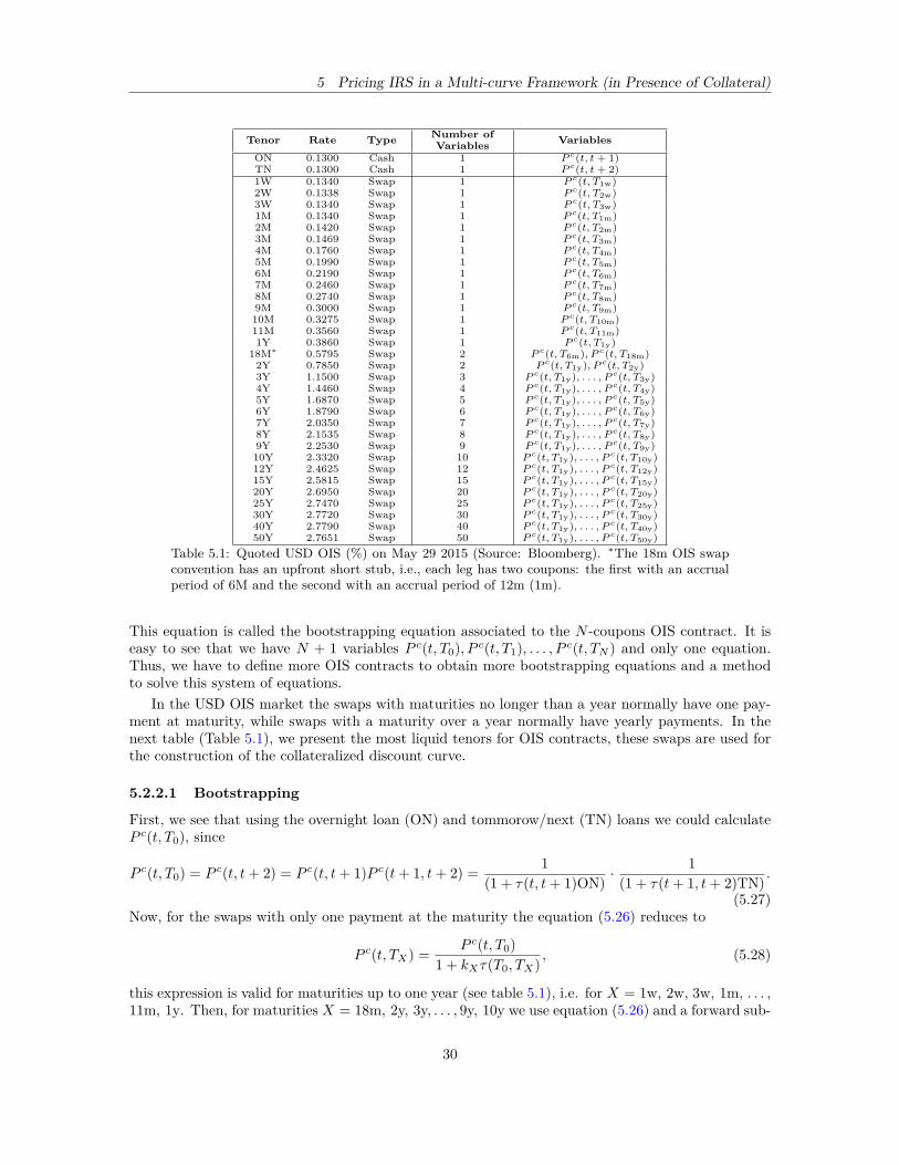
5 Pricing IRS in a Multi-curve Framework (in Presence of Collateral)
Tenor Rate Type Number ofVariables Variables
ON 0.1300 Cash 1 P c(t, t+ 1)TN 0.1300 Cash 1 P c(t, t+ 2)1W 0.1340 Swap 1 P c(t, T1w)2W 0.1338 Swap 1 P c(t, T2w)3W 0.1340 Swap 1 P c(t, T3w)1M 0.1340 Swap 1 P c(t, T1m)2M 0.1420 Swap 1 P c(t, T2m)3M 0.1469 Swap 1 P c(t, T3m)4M 0.1760 Swap 1 P c(t, T4m)5M 0.1990 Swap 1 P c(t, T5m)6M 0.2190 Swap 1 P c(t, T6m)7M 0.2460 Swap 1 P c(t, T7m)8M 0.2740 Swap 1 P c(t, T8m)9M 0.3000 Swap 1 P c(t, T9m)
10M 0.3275 Swap 1 P c(t, T10m)11M 0.3560 Swap 1 P c(t, T11m)1Y 0.3860 Swap 1 P c(t, T1y)
18M∗ 0.5795 Swap 2 P c(t, T6m), P c(t, T18m)2Y 0.7850 Swap 2 P c(t, T1y), P c(t, T2y)3Y 1.1500 Swap 3 P c(t, T1y), . . . , P c(t, T3y)4Y 1.4460 Swap 4 P c(t, T1y), . . . , P c(t, T4y)5Y 1.6870 Swap 5 P c(t, T1y), . . . , P c(t, T5y)6Y 1.8790 Swap 6 P c(t, T1y), . . . , P c(t, T6y)7Y 2.0350 Swap 7 P c(t, T1y), . . . , P c(t, T7y)8Y 2.1535 Swap 8 P c(t, T1y), . . . , P c(t, T8y)9Y 2.2530 Swap 9 P c(t, T1y), . . . , P c(t, T9y)
10Y 2.3320 Swap 10 P c(t, T1y), . . . , P c(t, T10y)12Y 2.4625 Swap 12 P c(t, T1y), . . . , P c(t, T12y)15Y 2.5815 Swap 15 P c(t, T1y), . . . , P c(t, T15y)20Y 2.6950 Swap 20 P c(t, T1y), . . . , P c(t, T20y)25Y 2.7470 Swap 25 P c(t, T1y), . . . , P c(t, T25y)30Y 2.7720 Swap 30 P c(t, T1y), . . . , P c(t, T30y)40Y 2.7790 Swap 40 P c(t, T1y), . . . , P c(t, T40y)50Y 2.7651 Swap 50 P c(t, T1y), . . . , P c(t, T50y)
Table 5.1: Quoted USD OIS (%) on May 29 2015 (Source: Bloomberg). ∗The 18m OIS swapconvention has an upfront short stub, i.e., each leg has two coupons: the first with an accrualperiod of 6M and the second with an accrual period of 12m (1m).
This equation is called the bootstrapping equation associated to the N -coupons OIS contract. It iseasy to see that we have N + 1 variables P c(t, T0), P c(t, T1), . . . , P c(t, TN ) and only one equation.Thus, we have to define more OIS contracts to obtain more bootstrapping equations and a methodto solve this system of equations.
In the USD OIS market the swaps with maturities no longer than a year normally have one pay-ment at maturity, while swaps with a maturity over a year normally have yearly payments. In thenext table (Table 5.1), we present the most liquid tenors for OIS contracts, these swaps are used forthe construction of the collateralized discount curve.
5.2.2.1 Bootstrapping
First, we see that using the overnight loan (ON) and tommorow/next (TN) loans we could calculateP c(t, T0), since
P c(t, T0) = P c(t, t+ 2) = P c(t, t+ 1)P c(t+ 1, t+ 2) = 1(1 + τ(t, t+ 1)ON) ·
1(1 + τ(t+ 1, t+ 2)TN) .
(5.27)Now, for the swaps with only one payment at the maturity the equation (5.26) reduces to
P c(t, TX) = P c(t, T0)1 + kXτ(T0, TX) , (5.28)
this expression is valid for maturities up to one year (see table 5.1), i.e. for X = 1w, 2w, 3w, 1m, . . . ,11m, 1y. Then, for maturities X = 18m, 2y, 3y, . . . , 9y, 10y we use equation (5.26) and a forward sub-
30
5 Pricing IRS in a Multi-curve Framework (in Presence of Collateral)
stitution to obtain the values of P c(t, TX) for all X. So far we have obtained discount factors withoutusing the bootstrapping method. However it is easy to see that equation (5.26) for the maturity of12y has two unknown variables: P c(t, T11y) and P c(t, T12y). That leads us to a single equation withtwo variables, we use the bootstrapping method to resolve this issue. The idea of bootstrapping isto make an initial guess for the variable P c0 (t, T12y)15 and with an interpolation method calculate thevalue of P c0 (t, T11y). It is important to mention that in the financial industry is commonly seen thatthe initial guess and interpolation is done in zero coupon rates. Therefore, for the case of maturity of12y, first we make an initial guess for the zero coupon rate Rc0(t, T12y) and then calculate Rc0(t, T11y)by interpolation. We calculate the discount factors P c0 (t, T11y) and P c0 (t, T12y) using these zero rates.Then we assume that P c0 (t, T11y) is “correct”16 and we calculate the “real” value of P c1 (t, T12y) using(5.26), i.e.,
P c1 (t, T12y) =P c(t, T0)− k12y
∑10i=1 τ(T(i−1)y, Tiy)P c(t, Ti)− k12yτ(T10y, T11y)P c0 (t, T11y)
1 + k12yτ(T11y, T12y) . (5.29)
Next we calculate the new value of Rc1(t, T12y) using P c1 (t, T12y), also we calculate and Rc1(t, T11y)again with the interpolation method. We iterate this procedure until it converges. For instance, thestop condition is given as
|P ci+1(t, T12y)− P ci (t, T12y)| < ε, ε > 0, (5.30)
Additionally, it is convenient to include a maximum number of iteration, i.e., iterate until one of thefollowing conditions is met,
|P ci+1(t, T12y)− P ci (t, T12y)| < ε, ε > 0 or i > Nmax > 0. (5.31)
This bootstrapping method is used similarly for all the OISs maturities up to 50y. In the appendixD we present a pseudocode for the bootstrapping of the USD OIS Curve.
Remark 5.2. Yield rates or zero rates in this work are treated as continuously compounded rates,i.e.
P (t, T ) = e−τ(t,T )R(t,T ). (5.32)
Using the data displayed in table 5.1 we build in R the OIS yield curve and the discount curve.The resulting calibrated curves are presented in the next charts 5.2 and 5.3, where additionally areincluded the curves that we obtained using the software SuperDerivatives, see table E.1.
15The subscript number 0 indicates that the number is an initial condition or an initial guess. If the subscript is anumber i, then it would indicates the number of iteration.
16We write “correct” since this value depends directly in the assumptions of the model, the instruments involved in itand naturally the interpolation. Recall that many choices of interpolation functions are possible and, according to thenature of the problem, we impose requirements such as: continuity, differentiability, twice differentiability, conditionsat the boundary, and so on.
31
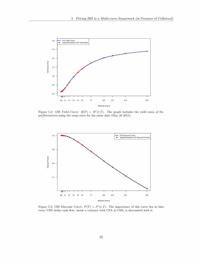
5 Pricing IRS in a Multi-curve Framework (in Presence of Collateral)
0.0
0.5
1.0
1.5
2.0
2.5
3.0
Maturity (years)
Yie
ld C
urve
(%
)
1M 1Y 2Y 3Y 4Y 5Y 7Y 10Y 12Y 15Y 20Y
OIS Yield CurveSuperDerivatives OIS Yield Rates
Figure 5.2: OIS Yield Curve: R(T ) = Rc(t, T ). The graph includes the yield rates of Su-perDerivatives using the swap rates for the same date (May 29 2015).
0.7
0.8
0.9
1.0
Maturity (years)
Dis
coun
t Fac
tor
1M 1Y 2Y 3Y 4Y 5Y 7Y 10Y 12Y 15Y 20Y
OIS Discount CurveSuperDerivatives OIS Discount Factors
Figure 5.3: OIS Discount Curve: P (T ) = P c(t, T ). The importance of this curve lies in thatevery USD dollar cash flow, inside a contract with CSA in USD, is discounted with it.
32
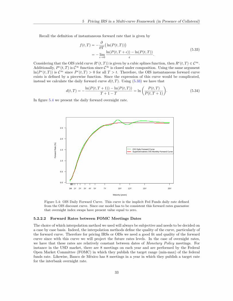
5 Pricing IRS in a Multi-curve Framework (in Presence of Collateral)
Recall the definition of instantaneous forward rate that is given by
f(t, T ) = − ∂
∂T
(ln(P (t, T ))
)= − lim
ε→0
ln(P (t, T + ε))− ln(P (t, T ))ε
.
(5.33)
Considering that the OIS yield curve Rc(t, T )) is given by a cubic splines function, then Rc(t, T ) ∈ C∞.Additionally, P c(t, T ) is C∞ function since C∞ is closed under composition. Using the same argumentln(P c(t, T )) is C∞ since P c(t, T ) > 0 for all T > t. Therefore, the OIS instantaneous forward curveexists is defined by a piecewise function. Since the expression of this curve would be complicated,instead we calculate the daily forward curve d(t, T ). Using (5.33) we have that
d(t, T ) = − ln(P (t, T + 1))− ln(P (t, T ))T + 1− T = ln
(P (t, T )
P (t, T + 1)
). (5.34)
In figure 5.4 we present the daily forward overnight rate.
0.0
0.5
1.0
1.5
2.0
2.5
Maturity (years)
For
war
d R
ate
(%)
1M 1Y 2Y 3Y 4Y 5Y 7Y 10Y 12Y 15Y 20Y
OIS Daily Forward CurveSuperDerivatives OIS Monthly Forward Curve
Figure 5.4: OIS Daily Forward Curve. This curve is the implicit Fed Funds daily rate definedfrom the OIS discount curve. Since our model has to be consistent this forward rates guaranteethat overnight index swaps have present value equal to zero.
5.2.2.2 Forward Rates between FOMC Meetings Dates
The choice of which interpolation method we used will always be subjective and needs to be decided ona case by case basis. Indeed, the interpolation methods define the quality of the curve, particularly ofthe forward curve. Therefore for pricing IRSs or OISs we need a good fit and quality of the forwardcurve since with this curve we will project the future rates levels. In the case of overnight rates,we have that these rates are relatively constant between dates of Monetary Policy meetings. Forinstance in the USD market, there are 8 meetings on each year and are performed by the FederalOpen Market Committee (FOMC) in which they publish the target range (min-max) of the federalfunds rate. Likewise, Banco de México has 8 meetings in a year in which they publish a target ratefor the interbank overnight rate.
33

5 Pricing IRS in a Multi-curve Framework (in Presence of Collateral)
Given the fact overnight rates, in particular the fed fund, are constant within a period of time somemodels are fitted to capture short-term monetary policy decisions. In [Clarke, 2010], Justin Clarkeused an additive seasonality adjustment for building the short dated portion of the OIS curve. Theidea is simple, he used market OIS quotes for pricing OISs with tenors equal the FOMC meeting datesand then keep constant these rates between meetings; the resulting forward curve is discontinuousin some short dated FOMC meetings. The longer term of the curve is calibrated using the simplebootstrapping presented above.
There are other models that use Federal Fund Futures to capture the probability of a rate cut orhike, see [Robertson et al., 1997], [Kuttner, 2001] and [Labuszewski and Newman, 2014]. However,for pricing purposes we could define a finite set of Monetary Policy scenarios with a probability thatcorresponds to a economical view. In figure 5.5, we present an example of a scenario of FOMC ratehikes. This scenario was defined on May 29 2015 with five 2015-FOMC meetings to go. The idea ofthe model is to price an IRSs for each scenario and then calculated the expected value using the givenprobabilities.
0.0
0.2
0.4
0.6
0.8
Dates
Dai
ly F
orw
ard
Rat
e (%
)
Jul 15 Sep 15 Nov 15 Jan 16 Mar 16 May 16
0.125%
0.375%
0.625%
0.125%
0.375%
0.625%
OIS Daily Forward RateFOMC MeetingsFOMC Mean Target Rate Example ScenarioFOMC Target Range (Upper Bound) Example ScenarioFOMC Target Range (Lower Bound) Example Scenario
Figure 5.5: FOMC Meetings and OIS forward curve and FOMC monetary policy scenario. Inthis chart we present the OIS forward curve calibrated when we perform a bootstrapping as insection. We also include a scenario of FOMC monetary policy decisions.
5.2.3 Calibration of the USD forward curve
In the previous section we explained the methodology used for the construction of the USD discountingcurve. We remind that this curve is extremely important because every cash flow denominated in USDcurrency is discounted with this curve on the assumption that the CSA agreement is in USD currency.In this section we present the methodology for building index forward curves. We only describe howto estimate the forward curve for LIBOR 3m and LIBOR 1m. For the construction of the forwardindex LIBOR 3m curve we use the plain vanilla IRS and for the forward index LIBOR 1m we useplain vanilla IRSs for the short-term of the curve and TS for the longer part. In tables , we presentthe maturities and swap rates that we will use for the forward curve calibration.
Let PV(t) be the present value of a payer IRS denominated in USD based on LIBOR 3m with
34
5 Pricing IRS in a Multi-curve Framework (in Presence of Collateral)
maturity of y years, hence
PV(t) =Qy∑i=1
α(ti−1, ti)Etit (LIBOR3M(ti−1, ti))P c(t, ti)− kySy∑j=1
β(sj−1, sj)P c(t, sj), (5.35)
where:ky: fixed rate of the plain vanilla interest rate swap with maturity in y yearsQy: number of quarters in y yearsSy: number of semesters in y yearsti, ti: coupon periods (start date, end date and payment date) for the floatinglegsj , sj : coupon periods (start date, end date and payment date) for the fixed legα(ti−1, ti)): accrual factor of the ith coupon of the floating leg (ACT/360)β(sj−1, sj)): accrual factor of the jth coupon of the fixed leg (30/360)P c(t, x): discount factors collateralized in USDEtit (LIBOR3M(ti−1, ti)): the LIBOR 3m forward rate of the ith coupon.
This swap with the above characteristics is the most plain vanilla IRS in the USD market. Itexchanges LIBOR 3m payable quarterly versus a semiannual fixed rate coupon with a day count of30/360 that is used primarily in government bonds. We say that it is the most plain vanilla since isthe most standard and liquid swap in the market.
Now, let us write Etit (LIBOR3M(ti−1, ti)) from equation (5.35) in terms of a discount17 curve,i.e.
Etit (LIBOR3M(ti−1, ti)) =(
1τ(ti−1, ti)
(P 3m(t, ti−1)P 3m(t, ti)
− 1))
, (5.36)
where τ(ti−1, ti) = τi is the day count convention to determine the year fraction for discounting andcurve building.
Substituting equation (5.36) into (5.35) and solving for P 3m(t, tQy ) yields
P 3m(t, tQy ) =P 3m(t, tQy−1)
1 +τi
(ky∑Sy
j=1βjP c(t,sj)−
∑Qy−1i=1
αiτi
(P3m(t,ti−1)P3m(t,ti)
−1)P c(t,ti)
)αiP c(t,tQy )
(5.37)
This equation allows us to find the discount curve based on LIBOR 3m using a simple bootstrap-ping and an interpolation method. The equation (5.37) seems more complicated than the previousbootstrapping equations nevertheless the iterative process is the same as in OIS-USD curve or as insingle-curve framework.
Once we have calibrated the forward LIBOR 3m curve we are able to build the LIBOR 1m for-ward curve. For the IRSs with maturities less than (or equal) 1 year, we could proceed for the curveconstruction exactly as in LIBOR 3m. Indeed, IRSs based on LIBOR 1m are quoted in the market forthese maturities and the plain vanilla convention is: the fixed leg has annual payments (ACT/360); thefloating leg has monthly payments with same day count convention. However for maturities greaterthan 1 year we have to use TSs quoted in the market that exchanges LIBOR 1m for LIBOR 3m. Letus present the bootstrapping equations for both cases.
17Note that the discount curve of LIBOR 3m is valid for discounting flows when the collateral rate is the LIBOR3m index. It is important to remind that for uncollateralized deals typically the discounting curve is the one based onLIBOR 3m i.e. P 3m(t, x).
35
5 Pricing IRS in a Multi-curve Framework (in Presence of Collateral)
Suppose we enter into a payer short-term IRS (maturities of 2m, 3m, 4m, . . . , 12m) based onLIBOR 1m. For these swaps the fixed leg has only one coupon at maturity. The present value of theIRS is given by
PV(t) =M∑i=1
α(ti−1, ti)Etit (LIBOR1M(ti−1, ti))P c(t, ti)− kMβ(t0, tM )P c(t, tM ), (5.38)
where:kM : fixed rate of the plain vanilla IRS with M couponsM : number of months (and coupons in floating leg) of the IRSti, ti: coupon periods for the floating legt0, tM : start date and end date of the IRSα(ti−1, ti)): accrual factor of the ith coupon of the floating leg (ACT/360)β(t0, tM )): accrual factor of the fixed leg coupon (ACT/360)P c(t, x): discount factors collateralized in USDEtit (LIBOR1M(ti−1, ti)): the LIBOR 1m forward rate of the ith coupon.
Note that by setting equation (5.38) equal to zero and solving for EtMt (LIBOR1M(tM−1, tM ))yields,
EtMt (LIBOR1M(tM−1, tM )) =kMβ0,MP
c(t, tM )−∑M−1i=1 αiEtit (LIBOR1M(ti−1, ti))P c(t, ti)αMP c(t, tM )
(5.39)Now, for maturity of 2m the forward rate of LIBOR 1m is easily determined since all the right side ofequation is known. Taking advantage that the quotes of IRSs based on LIBOR 1m are available forevery month then we could get all forward LIBOR 1m rates up to one year by forward substitutionusing equation (5.39). Now for maturities greater than one year we use TSs quoted in the market.Recall that the most popular TSs in the USD market are: 1m vs 3m, 3m vs 6m and 3m vs 12m. All ofthem are traded against LIBOR 3m since it is the most liquid and traded IRSs, see table 5.2. The TSspread should be positive, hence it is required to be added in the shorter tenor leg. Also, the paymentfrequency is determined by the longer tenor. In this work we only focus on the LIBOR 1m vs LIBOR3m TS.
Let PV(t) be the present value of a payer TS that exchanges LIBOR 1m with LIBOR 3m. Sincethe longer tenor is three months then both legs pay in a quarterly basis the coupons of the TS withthe same business day calendar and the same day count convention ACT/360. Considering that theLIBOR 1m fixing is typically payable every month, we need to compound this monthly payments andpay them quarterly18. Hence, following equations (3.15)-(3.16) of section 3.2 we have that the presentvalue is given by
PV(t) =M∑i=1
α(ti−1, ti)Etit (LIBOR3M(ti−1, ti))P c(t, ti)
−M∑i=1
α(ti−1, ti)[
1∑Nij=1 β(sj−1, sj)
( Ni∏j=1
(1 + β(sj−1, sj)E
sjt (LIBOR1M(sj−1, sj))
))
+BM
]P c(t, ti)
(5.40)
18There exist various types for compounding rates, in the plain vanilla TS the market convention is to use thecompounding with simple spread i.e. compound the rates and then apply the spread. The other two commonly usedtypes of spread are: 1) Compounding with spread in which the spread is applied to the rate and then we compoundthem; 2) Flat compounding in which we applied the spread before the compounding and also we consider the interestsof the previous coupons while compounding. See [ISDA, 2009].
36
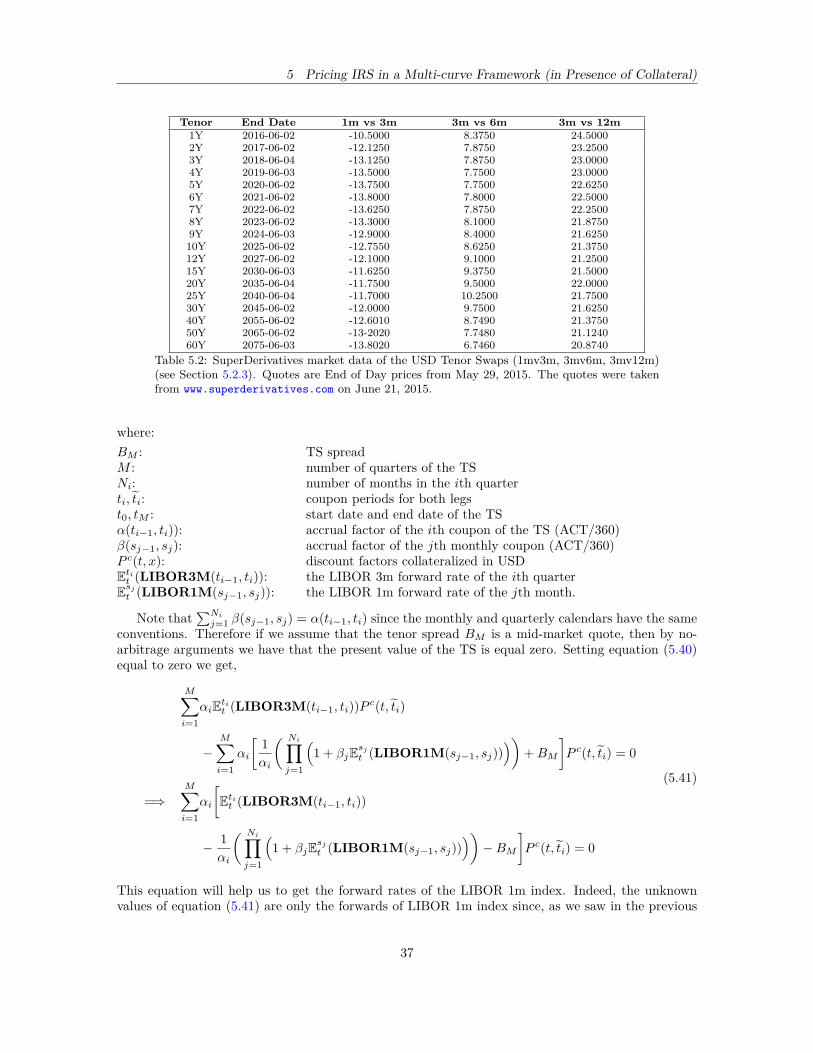
5 Pricing IRS in a Multi-curve Framework (in Presence of Collateral)
Tenor End Date 1m vs 3m 3m vs 6m 3m vs 12m1Y 2016-06-02 -10.5000 8.3750 24.50002Y 2017-06-02 -12.1250 7.8750 23.25003Y 2018-06-04 -13.1250 7.8750 23.00004Y 2019-06-03 -13.5000 7.7500 23.00005Y 2020-06-02 -13.7500 7.7500 22.62506Y 2021-06-02 -13.8000 7.8000 22.50007Y 2022-06-02 -13.6250 7.8750 22.25008Y 2023-06-02 -13.3000 8.1000 21.87509Y 2024-06-03 -12.9000 8.4000 21.625010Y 2025-06-02 -12.7550 8.6250 21.375012Y 2027-06-02 -12.1000 9.1000 21.250015Y 2030-06-03 -11.6250 9.3750 21.500020Y 2035-06-04 -11.7500 9.5000 22.000025Y 2040-06-04 -11.7000 10.2500 21.750030Y 2045-06-02 -12.0000 9.7500 21.625040Y 2055-06-02 -12.6010 8.7490 21.375050Y 2065-06-02 -13-2020 7.7480 21.124060Y 2075-06-03 -13.8020 6.7460 20.8740
Table 5.2: SuperDerivatives market data of the USD Tenor Swaps (1mv3m, 3mv6m, 3mv12m)(see Section 5.2.3). Quotes are End of Day prices from May 29, 2015. The quotes were takenfrom www.superderivatives.com on June 21, 2015.
where:BM : TS spreadM : number of quarters of the TSNi: number of months in the ith quarterti, ti: coupon periods for both legst0, tM : start date and end date of the TSα(ti−1, ti)): accrual factor of the ith coupon of the TS (ACT/360)β(sj−1, sj): accrual factor of the jth monthly coupon (ACT/360)P c(t, x): discount factors collateralized in USDEtit (LIBOR3M(ti−1, ti)): the LIBOR 3m forward rate of the ith quarterEsjt (LIBOR1M(sj−1, sj)): the LIBOR 1m forward rate of the jth month.
Note that∑Nij=1 β(sj−1, sj) = α(ti−1, ti) since the monthly and quarterly calendars have the same
conventions. Therefore if we assume that the tenor spread BM is a mid-market quote, then by no-arbitrage arguments we have that the present value of the TS is equal zero. Setting equation (5.40)equal to zero we get,
M∑i=1
αiEtit (LIBOR3M(ti−1, ti))P c(t, ti)
−M∑i=1
αi
[1αi
( Ni∏j=1
(1 + βjE
sjt (LIBOR1M(sj−1, sj))
))+BM
]P c(t, ti) = 0
=⇒M∑i=1
αi
[Etit (LIBOR3M(ti−1, ti))
− 1αi
( Ni∏j=1
(1 + βjE
sjt (LIBOR1M(sj−1, sj))
))−BM
]P c(t, ti) = 0
(5.41)
This equation will help us to get the forward rates of the LIBOR 1m index. Indeed, the unknownvalues of equation (5.41) are only the forwards of LIBOR 1m index since, as we saw in the previous
37
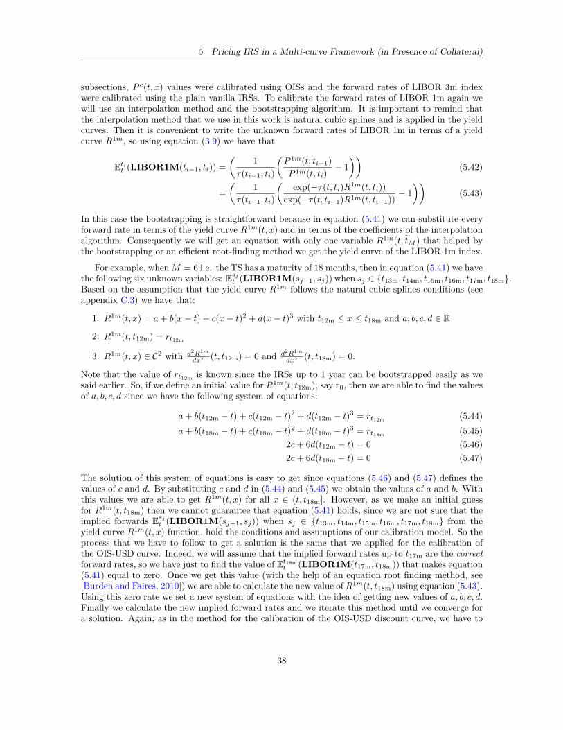
5 Pricing IRS in a Multi-curve Framework (in Presence of Collateral)
subsections, P c(t, x) values were calibrated using OISs and the forward rates of LIBOR 3m indexwere calibrated using the plain vanilla IRSs. To calibrate the forward rates of LIBOR 1m again wewill use an interpolation method and the bootstrapping algorithm. It is important to remind thatthe interpolation method that we use in this work is natural cubic splines and is applied in the yieldcurves. Then it is convenient to write the unknown forward rates of LIBOR 1m in terms of a yieldcurve R1m, so using equation (3.9) we have that
Etit (LIBOR1M(ti−1, ti)) =(
1τ(ti−1, ti)
(P 1m(t, ti−1)P 1m(t, ti)
− 1))
(5.42)
=(
1τ(ti−1, ti)
(exp(−τ(t, ti)R1m(t, ti))
exp(−τ(t, ti−1)R1m(t, ti−1)) − 1))
(5.43)
In this case the bootstrapping is straightforward because in equation (5.41) we can substitute everyforward rate in terms of the yield curve R1m(t, x) and in terms of the coefficients of the interpolationalgorithm. Consequently we will get an equation with only one variable R1m(t, tM ) that helped bythe bootstrapping or an efficient root-finding method we get the yield curve of the LIBOR 1m index.
For example, whenM = 6 i.e. the TS has a maturity of 18 months, then in equation (5.41) we havethe following six unknown variables: Esjt (LIBOR1M(sj−1, sj)) when sj ∈ t13m, t14m, t15m, t16m, t17m, t18m.Based on the assumption that the yield curve R1m follows the natural cubic splines conditions (seeappendix C.3) we have that:
1. R1m(t, x) = a+ b(x− t) + c(x− t)2 + d(x− t)3 with t12m ≤ x ≤ t18m and a, b, c, d ∈ R
2. R1m(t, t12m) = rt12m
3. R1m(t, x) ∈ C2 with d2R1m
dx2 (t, t12m) = 0 and d2R1m
dx2 (t, t18m) = 0.
Note that the value of rt12m is known since the IRSs up to 1 year can be bootstrapped easily as wesaid earlier. So, if we define an initial value for R1m(t, t18m), say r0, then we are able to find the valuesof a, b, c, d since we have the following system of equations:
a+ b(t12m − t) + c(t12m − t)2 + d(t12m − t)3 = rt12m (5.44)a+ b(t18m − t) + c(t18m − t)2 + d(t18m − t)3 = rt18m (5.45)
2c+ 6d(t12m − t) = 0 (5.46)2c+ 6d(t18m − t) = 0 (5.47)
The solution of this system of equations is easy to get since equations (5.46) and (5.47) defines thevalues of c and d. By substituting c and d in (5.44) and (5.45) we obtain the values of a and b. Withthis values we are able to get R1m(t, x) for all x ∈ (t, t18m]. However, as we make an initial guessfor R1m(t, t18m) then we cannot guarantee that equation (5.41) holds, since we are not sure that theimplied forwards Esjt (LIBOR1M(sj−1, sj)) when sj ∈ t13m, t14m, t15m, t16m, t17m, t18m from theyield curve R1m(t, x) function, hold the conditions and assumptions of our calibration model. So theprocess that we have to follow to get a solution is the same that we applied for the calibration ofthe OIS-USD curve. Indeed, we will assume that the implied forward rates up to t17m are the correctforward rates, so we have just to find the value of Et18m
t (LIBOR1M(t17m, t18m)) that makes equation(5.41) equal to zero. Once we get this value (with the help of an equation root finding method, see[Burden and Faires, 2010]) we are able to calculate the new value of R1m(t, t18m) using equation (5.43).Using this zero rate we set a new system of equations with the idea of getting new values of a, b, c, d.Finally we calculate the new implied forward rates and we iterate this method until we converge fora solution. Again, as in the method for the calibration of the OIS-USD discount curve, we have to
38
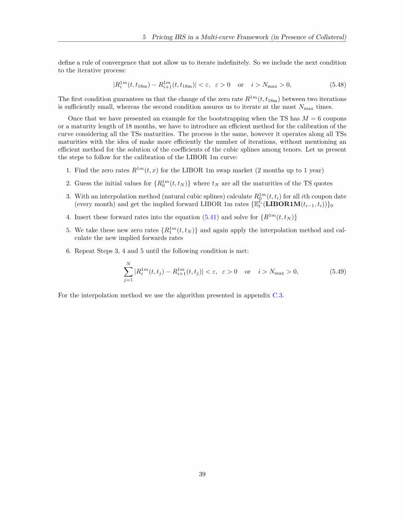
5 Pricing IRS in a Multi-curve Framework (in Presence of Collateral)
define a rule of convergence that not allow us to iterate indefinitely. So we include the next conditionto the iterative process:
|R1mi (t, t18m)−R1m
i+1(t, t18m)| < ε, ε > 0 or i > Nmax > 0, (5.48)
The first condition guarantees us that the change of the zero rate R1m(t, t18m) between two iterationsis sufficiently small, whereas the second condition assures us to iterate at the most Nmax times.
Once that we have presented an example for the bootstrapping when the TS has M = 6 couponsor a maturity length of 18 months, we have to introduce an efficient method for the calibration of thecurve considering all the TSs maturities. The process is the same, however it operates along all TSsmaturities with the idea of make more efficiently the number of iterations, without mentioning anefficient method for the solution of the coefficients of the cubic splines among tenors. Let us presentthe steps to follow for the calibration of the LIBOR 1m curve:
1. Find the zero rates R1m(t, x) for the LIBOR 1m swap market (2 months up to 1 year)
2. Guess the initial values for R1m0 (t, tN ) where tN are all the maturities of the TS quotes
3. With an interpolation method (natural cubic splines) calculate R1m0 (t, ti) for all ith coupon date
(every month) and get the implied forward LIBOR 1m rates Etit (LIBOR1M(ti−1, ti))0
4. Insert these forward rates into the equation (5.41) and solve for R1m(t, tN )
5. We take these new zero rates R1m1 (t, tN ) and again apply the interpolation method and cal-
culate the new implied forwards rates
6. Repeat Steps 3, 4 and 5 until the following condition is met:
N∑j=1|R1mi (t, tj)−R1m
i+1(t, tj)| < ε, ε > 0 or i > Nmax > 0, (5.49)
For the interpolation method we use the algorithm presented in appendix C.3.
39
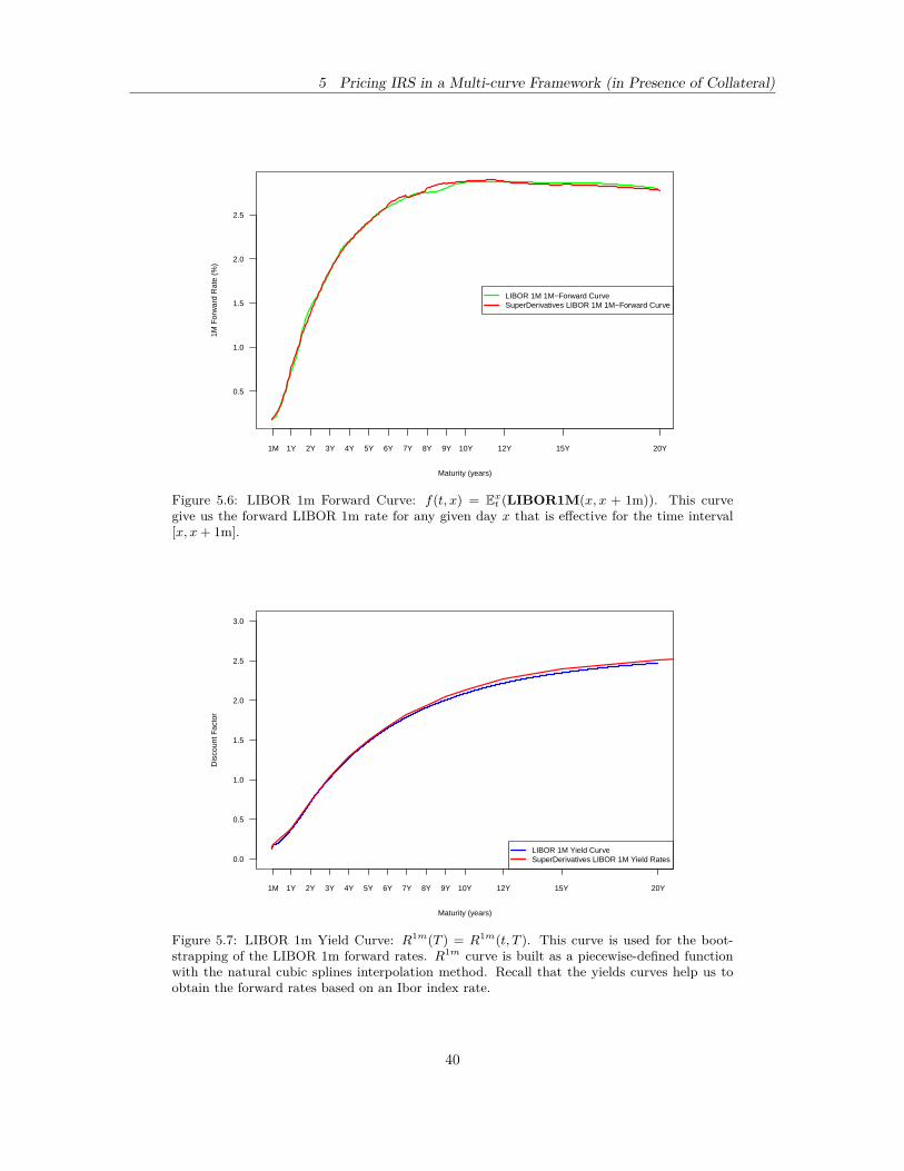
5 Pricing IRS in a Multi-curve Framework (in Presence of Collateral)
0.5
1.0
1.5
2.0
2.5
Maturity (years)
1M F
orw
ard
Rat
e (%
)
1M 1Y 2Y 3Y 4Y 5Y 6Y 7Y 8Y 9Y 10Y 12Y 15Y 20Y
LIBOR 1M 1M−Forward CurveSuperDerivatives LIBOR 1M 1M−Forward Curve
Figure 5.6: LIBOR 1m Forward Curve: f(t, x) = Ext (LIBOR1M(x, x + 1m)). This curve
give us the forward LIBOR 1m rate for any given day x that is effective for the time interval[x, x + 1m].
0.0
0.5
1.0
1.5
2.0
2.5
3.0
Maturity (years)
Dis
coun
t Fac
tor
1M 1Y 2Y 3Y 4Y 5Y 6Y 7Y 8Y 9Y 10Y 12Y 15Y 20Y
LIBOR 1M Yield CurveSuperDerivatives LIBOR 1M Yield Rates
Figure 5.7: LIBOR 1m Yield Curve: R1m(T ) = R1m(t, T ). This curve is used for the boot-strapping of the LIBOR 1m forward rates. R1m curve is built as a piecewise-defined functionwith the natural cubic splines interpolation method. Recall that the yields curves help us toobtain the forward rates based on an Ibor index rate.
40
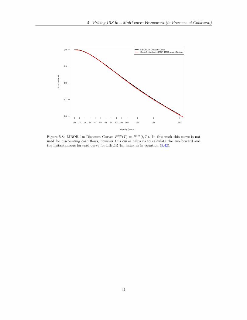
5 Pricing IRS in a Multi-curve Framework (in Presence of Collateral)
0.6
0.7
0.8
0.9
1.0
Maturity (years)
Dis
coun
t Fac
tor
1M 1Y 2Y 3Y 4Y 5Y 6Y 7Y 8Y 9Y 10Y 12Y 15Y 20Y
LIBOR 1M Discount CurveSuperDerivatives LIBOR 1M Discount Factors
Figure 5.8: LIBOR 1m Discount Curve: P 1m(T ) = P 1m(t, T ). In this work this curve is notused for discounting cash flows, however this curve helps us to calculate the 1m-forward andthe instantaneous forward curve for LIBOR 1m index as in equation (5.42).
41
5 Pricing IRS in a Multi-curve Framework (in Presence of Collateral)
5.3 Valuation Framework in Multiple CurrenciesWe saw before that the collateral determines the discount rate, i.e. a USD swap which is collateral-ized (cash) in USD is priced using the OIS (Fed Funds) curve. Now we have to answer the followingquestion: what if the swap is collateralized in EUR? And in JPY?
Let V (j) be the value collateral account for a derivative X in terms of currency (j). The stochasticprocess of the collateral account is given by
dV (j)(s) =(r(j)(s)− c(j)(s)
)V (j)(s)ds+ a(s)d
(h(i)(s) · f i→j(s)
), (5.50)
where, r(j)(s) and c(j)(s) are the risk-free rate and the collateral rate at time s of currency (j), re-spectively, h(i)(s) is the value of the derivative X in terms of currency (i) that matures at time T withcash flow h(i)(T ), f i→j(s) is the foreign exchange (FX) rate at time s representing the price of theunit amount of currency (i) in terms of currency (j). Finally, a(s) represents the number of positionsof the derivative at time s. To solve (5.50) we have to multiply the equation by e
∫ Tsy(j)(η)dη, where
y(j)(s) = r(j)(s)− c(j)(s), and we get
e
∫ Tsy(j)(η)dη
dV (j)(s) = e
∫ Tsy(j)(η)dη
y(j)(s)V (j)(s)ds+ e
∫ Tsy(j)(η)dη
a(s)d(h(i)(s) · f i→j(s)
). (5.51)
Then, by integrating (5.51) we have∫ T
t
e
∫ Tsy(j)(η)dη
dV (j)(s) =∫ T
t
e
∫ Tsy(j)(η)dη
y(j)(s)V (j)(s)ds+∫ T
t
e
∫ Tsy(j)(η)dη
a(s)d(h(i)(s)·f i→j(s)
).
(5.52)Let define u = e
∫ Tsy(j)(η)dη and dv = dV (j)(s), using integration by parts formula we obtain∫
udv = uv −∫vdu (5.53)∫ T
t
e
∫ Tsy(j)(η)dη
dV (j)(s) = e
∫ Tsy(j)(η)dη
V (j)(s)∣∣∣Tt
+∫ T
t
V (j)(s)e∫ Tsy(j)(η)dη
y(j)(s)ds. (5.54)
Then, using (5.52) and (5.54) we get
V (j)(T ) = e
∫ Tty(j)(η)dη
V (j)(t) +∫ T
t
e
∫ Tsy(j)(η)dη
a(s)d(h(i)(s) · f i→j(s)
). (5.55)
As in [Fujii et al., 2010b], by adopting the trading strategy specified byV (j)(t) = h(i)(t) · f i→j(t)
a(s) = e
∫ sty(j)(η)dη
(5.56)
By substituting the trading strategy in (5.55) we obtain
V (j)(T ) = e
∫ Tty(j)(η)dη
V (j)(t) +∫ T
t
e
∫ Tsy(j)(η)dη
a(s)d(h(i)(s) · f i→j(s)
)= e
∫ Tty(j)(η)dη
h(i)(t) · f i→j(t) +∫ T
t
e
∫ Tsy(j)(η)dη+
∫ sty(j)(η)dη
d(h(i)(s) · f i→j(s)
)= e
∫ Tty(j)(η)dη
h(i)(t) · f i→j(t) + e
∫ Tty(j)(η)dη
∫ T
t
d(h(i)(s) · f i→j(s)
)= e
∫ Tty(j)(η)dη
h(i)(t) · f i→j(t) + e
∫ Tty(j)(η)dη
((h(i)(T ) · f i→j(T )
)−(h(i)(t) · f i→j(t)
))= e
∫ Tty(j)(η)dη(
h(i)(T ) · f i→j(T )). (5.57)
42
5 Pricing IRS in a Multi-curve Framework (in Presence of Collateral)
Now we have that,
h(i)(T ) = V (j)(T )f j→i(T )e−∫ Tty(j)(η)dη = V (i)(T )e−
∫ Tty(j)(η)dη
. (5.58)
We are able to compute the present value of h(i)(t) of the derivative X using the risk neutral measureQ(i) associated to the numéraire (money-market account) B(i)(t) = e
∫ Ttr(i)(s)ds,i.e.,
h(i)(t) = EQ(i)t
[V (i)(T )B(i)(T )
]= EQ(i)
t
[(e−∫ Ttr(i)(s)ds)(
e
∫ Tty(j)(s)ds)
h(i)(T )]
(5.59)
If we define y(i,j)(s) = y(i)(s)− y(j)(s) then we could express h(i)(t) as follows
h(i)(t) = EQ(i)t
[(e−∫ Ttr(i)(s)ds)(
e
∫ Tty(j)(s)ds)
h(i)(T )]
= EQ(i)t
[(e−∫ Ttc(i)(s)ds)]ETc(i)
t
[(e−∫ Tty(i,j)(s)ds)
h(i)(T )]
= P c(i)(t, T )ETc(i)t
[(e−∫ Tty(i,j)(s)ds)
h(i)(T )], (5.60)
where P c(i)(t, T ) is the collateralized zero coupon bond of currency (i) and Tc(i) is the collateralizedforward measure of the same currency where P c(i)(t, T ) is used as numéraire. Note that when (i) = (j)
then from (5.60) we have that h(i)(t) = P c(i)(t, T )ETc(i)t
[h(i)(T )
]which coincides with equation (5.18).
In the next subsection we will present the differences between pricing IRSs denominated in EURand MXN when the collateral currency is USD. We will see that the existence of an OISs market easesthe curve construction.
5.3.1 Case of EUR
We have already built curves in USD, therefore the next step is to build curves in other currency—namely EUR— but keeping the same collateral currency (in this case USD). The EUR interestrate market instruments are mostly collateralized in EUR. In this market the overnight rate is calledEonia (acronym of Euro OverNight Index Average), and the OISs based on Eonia have the samecharacteristics of the OISs based on Fed Funds in the USD market.
Therefore with a list of EUR cash deposits and OISs swaps based on Eonia we are able to buildand calibrate —using a simple bootstrapping— the EUR discount curve when the cash flows are col-lateralized in EUR. In fact, the methodology is identical to the one used in section 5.2.2 to build USDdiscount curve. Once we have the discount curve (collateralized in EUR) we can use quotes from theEUR market based on the two dominant tenors: EURIBOR 3m and EURIBOR 6m; to build bothforward curves. For EURIBOR 3m curve we use short-term interest rates (STIR) futures and tenorbasis swaps (6m vs 3m), while for EURIBOR 6m we use forward rates agreements (FRAs) and vanillaIRSs.
Remark 5.3. As in USD market, EUR curves (Eonia (discount) EURIBOR 3m (forward) and EU-RIBOR 6m (forward)) can be build one by one with simple bootstrappings. The order is discounting,forward 6m and forward 3m.
43
5 Pricing IRS in a Multi-curve Framework (in Presence of Collateral)
Now to build the discount curves of EUR when the collateral is USD or vice versa we need theXCSs market. Recall that a plain vanilla EURUSD XCS exchanges LIBOR 3m flat for EURIBOR3m plus an additional spread, as is mention on section 3.2.4. In the interest rate market there existstwo types of XCSs: cnXCSs (constant notional XCSs) and mtmXCSs (mark-to-market XCSs)19, seesection 3.2.4. In a cnXCS the notionals of both legs are fixed using a FX rate agreed in the inception ofthe trade and kept constant until its maturity despite the FX rate moves. On the contrary, a mtmXCSresets the notional of one leg at the start of every coupon period (including the final notional exchange)while the other leg notional keeps constant. Even though the mtmXCS have better liquidity in almostevery currency, in this work we will asume that the XCSs have constant notionals due to USDMXNXCSs are still quoted with constant notionals. Therefore consider a cnXCS of a pair of currencies(i, j) and assume that the collateral is posted in currency j. Then the net present value of leg j iscalculated as: (suppose that the payment dates and coupon accrual periods are the same for bothlegs)20
Leg(j)(t) = N(j)
[− P c(j)(t, t0) + P c(j)(t, tN )
+N∑k=1
β(tk−1, tk)P c(j)(t, tk)ETc(j),kt
[L(j)(tk−1, tk)
]].
(5.61)
where:N(j): notional of j−currency legN : number of coupons(tk−1, tk): period of kth coupontk: time of payment of the kth coupon or notional exchangeβ(tk−1, tk): accrual factor of the kth couponETc(j),kt
[L(j)(tk−1, tk)
]: the j−forward reference rate of the kth coupon
P c(j)(t, tk): j−currency discount factor collateralized in j for time tk.
Now, using equation (5.60) we have that the net present value of leg i is
Leg(i)(t) = N(i)
[− P c(i)(t, t0)E
Tc(i),0t
[e−∫ t0ty(i,j)(s)ds]
+ P c(i)(t, tN )ETc(i),Nt
[e−∫ tNt
y(i,j)(s)ds]+
N∑k=1
β(tk−1, tk)P c(i)(t, tk)ETc(i),kt
[(L(i)(tk−1, tk) +BN
)e−∫ tkt
y(i,j)(s)ds]].
(5.62)
where:N(i): notional of i−currency legN : number of couponsBN : basis spread of the cnXCS with N coupons(tk−1, tk): period of kth coupontk: time of payment of the kth coupon or notional exchangeβ(tk−1, tk): accrual factor of the kth couponP c(i)(t, tk): i−currency discount factor collateralized in i for time tk
ETc(i),kt
[L(i)(tk−1, tk)e−
∫ tkt
y(i,j)(s)ds]: the i−forward reference rate of the kth coupon when the col-lateral currency is j.
19Also classified as: resettable XCSs or non-resetable XCSs, since the reset of the notional amount.20This assumption is, in fact, true for plain vanilla XCSs, i.e. the payment calendars for both legs coincide, either
the day count conventions.
44
5 Pricing IRS in a Multi-curve Framework (in Presence of Collateral)
Consider that we enter in a payer cnXCS i.e. we pay the leg with the basis spread BN , hence the netpresent value at time t of the contract in terms of currency j is given by
cnXCS(i,j)Payer(t) = Leg(j)(t)− f i→j(t, t0)Leg(i)(t), (5.63)
where f i→j(t, t0) is the spot FX rate.
For the curve construction, we can assume that N(j) = 1 and N(j) = N(i)fi→j(t, t0). Also, due
to the difference between the trade date and the start date, i.e. t0 − t is equal to 2 days and thecash deposits (overnight and tom-next) rates are nearly zero, then we can say that P c(j)(t, t0) ≈ 1 andP c(i)(t, t0) ≈ 1. Finally we will assume that y(i,j)(·) is a deterministic function, therefore by settingequation (5.63) equal to zero yields,
P c(j)(t, tN )− P c(i)(t, tN )f i→j(t, t0)P y(t, tN )
+N∑k=1
β(tk−1, tk)P c(j)(t, tk)ETc(j),Nt
[L(j)(tk−1, tk)
]− f i→j(t, t0)
N∑k=1
β(tk−1, tk)P c(i)(t, tk)[ETc(i),kt
[L(i)(tk−1, tk)
]+BN
]P y(t, tk) = 0
(5.64)
where P y(t, tk) = e−∫ tkt
y(i,j)(s)ds for all k = 0, 1, . . . , N . Note that when we assume that y(i,j) is a de-
terministic function then we are able to take out the term exp(−∫ tkty(i,j)(s)ds) from the expectation
of equation (5.62). Additionally, the terms
P c(i)(t, tk)P y(t, tk) (5.65)
could be interpreted as the discount factors of currency i fully collateralized in currency j.
So, the only unknown factors of equation (5.64) are the values of P y(t, tk). Hence using a boot-strapping with all the quotes of cnXCSs displayed in the market B(i, j)N and an interpolationmethod we can built the curve P y(t, T ) and thus y(i,j)(T ). We do not present results and animplementation of this bootstrapping since this work is focus on the MXN curve construction. Forinterested readers, see [Fujii et al., 2010a] for a deeper analysis of EURUSD and USDJPY XCSs.
5.3.2 Case of MXN
The main difference between EUR and MXN markets is the no existence of OISs in the latter. Besidesthat neither of the products IRSs nor XCSs are collateralized in MXN. Indeed they are collateralizedin USD. Nevertheless we have to propose a multi-curve framework for curve construction with theconstraints of replicating the market quotes considering the main currency of the CSA agreements.
According to the [MexDer, 2014], most of the banks in Mexico are funded with foreign capital andthey manage their books and trading desks outside Mexico. It is estimated that around 80% of theIRSs market operations are traded outside Mexico or by international (non-mexican) banks. For thisreason IRSs and XCSs (USDMXN) based on TIIE 28d are executed under a CSA agreement withUSD as collateral currency.
As we will see in section 6, neither the forward curve nor the discount curve could be obtainedwith a simple bootstrapping. In fact, we will present how to define a two-step bootstrapping to buildthe MXN forward curve (TIIE 28d as index rate) and the MXN discount curve collateralized in USD.In fact, the idea of this two-step bootstrapping is simple; we know that either the plain vanilla IRSsbased on TIIE 28d and plain vanilla XCSs that exchange LIBOR 1m plus a spread for TIIE 28d have
45
5 Pricing IRS in a Multi-curve Framework (in Presence of Collateral)
the same schedule i.e. coupons every 28 days with the following date convention and have the samematurities (84d, 168d, 252d and so on). However the spot lag is different since in IRSs it is of oneday whereas in XCSs it is of two days; also the payments calendars are MX and US-MX, respectively.These differences forbid us to substitute the MXN floating leg of the XCS for the fixed leg of the IRS.Nevertheless if we assume that this difference can be neglected then we can replace MXN floating legwith a fixed rate leg, thus the discounting curve of MXN leg collateralized in USD could be obtainedusing a simple bootstrapping. Then it is immediately followed the calibration of the forward curve(TIIE 28d) from the IRSs since the discounting curve collateralized in USD is known. This calibrationis again made by a simple bootstrapping. It is important to point out that in section 6 we will notassume that the spot lag and the calendars are equal in IRSs and XCSs, and, as a consequence, wewill have to iterate the bootstrappings to converge for a solution that replicates the market swaps:IRSs and XCSs.
In figure 5.9 we present a flowchart with the differences between the EUR and MXN markets andhow the USD market relates with them for the rate curves construction.
46
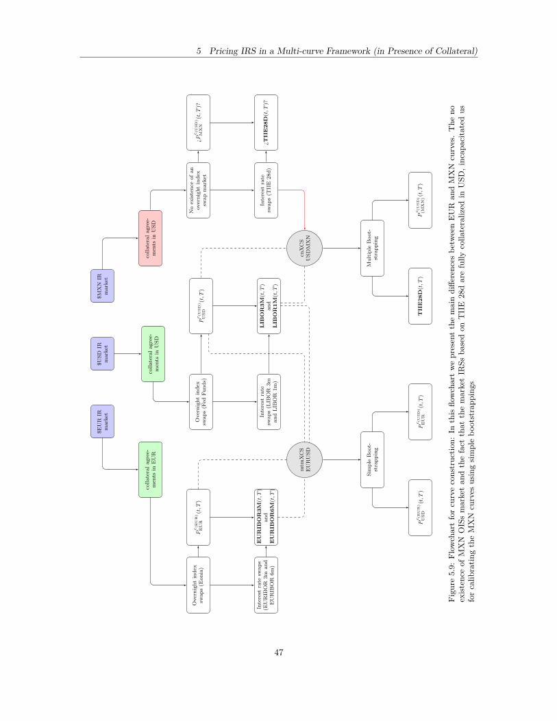
5 Pricing IRS in a Multi-curve Framework (in Presence of Collateral)
$USD
IRmarket
$EUR
IRmarket
$MXN
IRmarket
collateralagree-
men
tsin
EUR
collateralagree-
men
tsin
USD
collateralagree-
men
tsin
USD
Pc(EUR)
EUR
(t,T
)Overnightindex
swaps(E
onia)
Interest
rate
swaps
(EURIB
OR
3m
and
EURIB
OR
6m)
EURIB
OR3M
(t,T
)and
EURIB
OR6M
(t,T
)
Overnightindex
swaps(F
edFunds)
Pc(USD
)
USD
(t,T
)
Interest
rate
swaps(L
IBOR
3m
andLIB
OR
1m)
LIB
OR3M
(t,T
)and
LIB
OR1M
(t,T
)
Noex
istence
ofan
overnightindex
swapmarket
¿P
c(USD
)
MXN
(t,T
)?
Interest
rate
swaps(T
IIE
28d)
¿TIIE28D(t,T
)?
mtm
XCS
EURUSD
cnXCS
USDMXN
Sim
ple
Boot-
strapping
Multiple
Boot-
strapping
Pc(USD
)
EUR
(t,T
)P
c(EUR)
USD
(t,T
)P
c(USD
)
(MXN)(t,T
)TIIE28D(t,T
)
Figu
re5.9:
Flow
chartforcurveconstructio
n:In
thisflo
wchartwepresentthemaindiffe
rences
betw
eenEUR
andMXN
curves.The
noexistenceof
MXN
OISsmarketan
dthefact
that
themarketIR
Ssba
sedon
TIIE
28darefully
colla
teralized
inUSD
,incap
acita
tedus
forcalib
ratin
gtheMXN
curves
usingsimplebo
otstrapp
ings
47
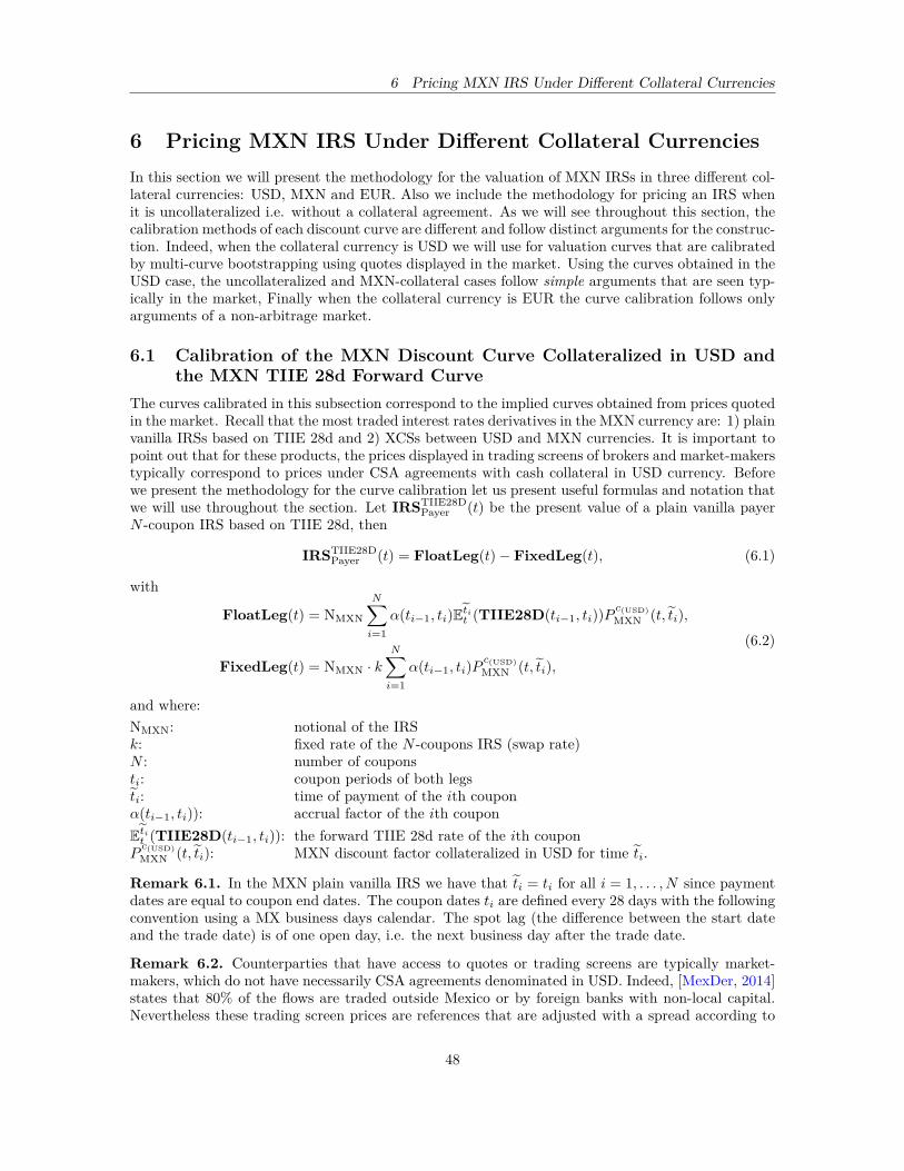
6 Pricing MXN IRS Under Different Collateral Currencies
6 Pricing MXN IRS Under Different Collateral CurrenciesIn this section we will present the methodology for the valuation of MXN IRSs in three different col-lateral currencies: USD, MXN and EUR. Also we include the methodology for pricing an IRS whenit is uncollateralized i.e. without a collateral agreement. As we will see throughout this section, thecalibration methods of each discount curve are different and follow distinct arguments for the construc-tion. Indeed, when the collateral currency is USD we will use for valuation curves that are calibratedby multi-curve bootstrapping using quotes displayed in the market. Using the curves obtained in theUSD case, the uncollateralized and MXN-collateral cases follow simple arguments that are seen typ-ically in the market, Finally when the collateral currency is EUR the curve calibration follows onlyarguments of a non-arbitrage market.
6.1 Calibration of the MXN Discount Curve Collateralized in USD andthe MXN TIIE 28d Forward Curve
The curves calibrated in this subsection correspond to the implied curves obtained from prices quotedin the market. Recall that the most traded interest rates derivatives in the MXN currency are: 1) plainvanilla IRSs based on TIIE 28d and 2) XCSs between USD and MXN currencies. It is important topoint out that for these products, the prices displayed in trading screens of brokers and market-makerstypically correspond to prices under CSA agreements with cash collateral in USD currency. Beforewe present the methodology for the curve calibration let us present useful formulas and notation thatwe will use throughout the section. Let IRSTIIE28D
Payer (t) be the present value of a plain vanilla payerN -coupon IRS based on TIIE 28d, then
IRSTIIE28DPayer (t) = FloatLeg(t)− FixedLeg(t), (6.1)
with
FloatLeg(t) = NMXN
N∑i=1
α(ti−1, ti)Etit (TIIE28D(ti−1, ti))Pc(USD)MXN (t, ti),
FixedLeg(t) = NMXN · kN∑i=1
α(ti−1, ti)Pc(USD)MXN (t, ti),
(6.2)
and where:NMXN: notional of the IRSk: fixed rate of the N -coupons IRS (swap rate)N : number of couponsti: coupon periods of both legsti: time of payment of the ith couponα(ti−1, ti)): accrual factor of the ith couponEtit (TIIE28D(ti−1, ti)): the forward TIIE 28d rate of the ith couponPc(USD)MXN (t, ti): MXN discount factor collateralized in USD for time ti.
Remark 6.1. In the MXN plain vanilla IRS we have that ti = ti for all i = 1, . . . , N since paymentdates are equal to coupon end dates. The coupon dates ti are defined every 28 days with the followingconvention using a MX business days calendar. The spot lag (the difference between the start dateand the trade date) is of one open day, i.e. the next business day after the trade date.
Remark 6.2. Counterparties that have access to quotes or trading screens are typically market-makers, which do not have necessarily CSA agreements denominated in USD. Indeed, [MexDer, 2014]states that 80% of the flows are traded outside Mexico or by foreign banks with non-local capital.Nevertheless these trading screen prices are references that are adjusted with a spread according to
48

6 Pricing MXN IRS Under Different Collateral Currencies
the collateral currency between the counterparties (valuation adjustment known as CollVA, see [Ruiz,2015]).
From equations (3.22)-(3.23)-(3.24) we have that the mark-to-market at time t (in MXN currency)of a plain vanilla payer USDMXN cnXCS (that exchanges LIBOR 1m plus a spread for TIIE 28d)cnXCSUSDMXN
Payer (t) is given by
cnXCSUSDMXNPayer (t) = LegMXN(t)− fUSD→MXN(t)LegUSD(t), (6.3)
with
LegMXN(t) = NMXN
[− P c(USD)
MXN (t, s0) + Pc(USD)MXN (t, sN )+
N∑j=1
β(sj−1, sj)Esjt (TIIE28D(sj−1, sj))P
c(USD)MXN (t, sj)
],
(6.4)
LegUSD(t) = NUSD
[− P c(USD)
USD (t, s0) + Pc(USD)USD (t, sN )+
N∑j=1
β(sj−1, sj)(Esjt (LIBOR1M(sj−1, sj)) +BN
)Pc(USD)USD (t, sj)
],
(6.5)
and fUSD→MXN(t) is the FX spot rate at time t. Additionally we have that,NUSD: notional of USD legNMXN: notional of MXN legN : number of couponsBN : basis spread of the N -coupons cnXCS(sj−1, sj): period of jth coupon (in both legs)sj : time of payment of the jth coupon (in both legs)β(sj−1, sj)): accrual factor of the jth coupon (in both legs)Esjt (LIBOR1M(sj−1, sj)): the forward LIBOR 1m rate of the jth couponEsjt (TIIE28D(sj−1, sj)): the forward TIIE 28d rate of the jth couponPc(USD)USD (t, sj): USD discount factor collateralized in USD for time sjPc(USD)MXN (t, sj): MXN discount factor collateralized in USD for time sj .
In the case of cnXCSs, no matter the number of coupons, we have that
NMXN = NUSDfUSD→MXN0 , (6.6)
where fUSD→MXN0 is the FX rate fixed by the two counterparties at the moment the deal is closed.
Note that in general fUSD→MXN0 6= fUSD→MXN(t), since the first one is used to determine the notional
of the MXN leg and the second is the FX spot rate used for the valuation of the mark-to-markets.However at the moment the trade is done counterparties agreed that the notionals are determineswith the FX spot rate, i.e. fUSD→MXN
0 = fUSD→MXN(t).
Remark 6.3. In a plain vanilla cnXCS the payment dates are scheduled every 28 days using thefollowing convention. However, in contrast with a plain vanilla IRS, these payment dates are deter-mined using an US-MX business days calendar and the spot lag is of two open days, i.e. the secondbusiness day after the trade date. Additionally we have that sj = sj for all j = 1, . . . , N .
Remark 6.4. For a plain vanilla TS that exchanges LIBOR 1m for LIBOR 3m, the fixings of theLIBOR 1m leg are determined on a monthly basis and the accrual factors too. However on the plainvanilla USDMXN cnXCS, the applicable accrual factor is calculated considering coupons of 28 days.
49

6 Pricing MXN IRS Under Different Collateral Currencies
Tenor Number ofCoupons (N)
Fixed Rate(%) Type Spread (%) Type
84D 3 3.3200 IRS 0.5400 cnXCS168D 6 3.4300 IRS 0.5900 cnXCS252D 9 3.5620 IRS 0.6400 cnXCS364D 13 3.7350 IRS 0.6800 cnXCS728D 26 4.2360 IRS 0.7200 cnXCS
1092D 39 4.6710 IRS 0.8100 cnXCS1456D 52 5.0510 IRS 0.8800 cnXCS1820D 65 5.3610 IRS 0.9200 cnXCS2548D 91 5.8630 IRS 1.0050 cnXCS3640D 130 6.2380 IRS 1.0400 cnXCS4368D 156 6.4280 IRS 1.0400 cnXCS5460D 195 6.6320 IRS 1.0200 cnXCS7280D 260 6.8310 IRS 1.0250 cnXCS
10920D 390 7.0210 IRS 1.0250 cnXCSTable 6.1: Quoted TIIE 28d IRSs and USDMXN cnXCSs on May 29 2015 (Source: Bloomberg).
From the previous sections we know how to build the USD discount curve collateralized in USDand the LIBOR 1m forward curve. Hence the values of P c(USD)
USD (t, x) and Ext (LIBOR1M(x, x+ 1m))in equation (6.5) are known for all x. So the remaining curves that we have to calibrate are
Pc(USD)MXN (t, x), and (6.7)
Ext (TIIE28D(x, x+ 28d)), for all x. (6.8)
Fortunately, we have two swap curves as inputs (IRS and cnXCS market quotes, see table 6.1) andwe have to solve two curves as outputs (discount of MXN collateralized in MXN and TIIE 28d indexcurve). Therefore, we get a kind of “system of equations” that may have a solution (not necessarilyunique) that can be found easily since it is a 2 × 2 “system of equations”21. Before we start tryingto solve this “system of equations” let us calculate the number of unknown variables. Note that thecnXCS with longest maturity (30 years) has 390 coupons (= 30 years × 13 coupons per year). Forevery MXN coupon we have two unknown variables: the discount factor and the forward index rate,hence we have 780 variables. However the TIIE 28d index rate for the first coupon is determined attime t so it is not an unknown variable. In summary, we have 779 variables and 28 equations (14 IRSand 14 cnXCS from table 6.1). Now it is clearly that the system of equations have infinite solutionsbut we have find the more simple and adequate solution that is consistent with the term structure ofthe interest rate market. This solution is obtained through an interpolation method and a multiplebootstrapping that builds iteratively the two curves at the same time. To illustrate the idea behindthis method let us suppose that our market only has one IRS and one cnXCS, both with maturityof 84 days. Also let us assume that NMXN = 1, hence the present value at time t of the IRS and thecnXCS (both payers) are given by,
IRSTIIE28DPayer (t) =
3∑i=1
α(ti−1, ti)Etit (TIIE28D(ti−1, ti))Pc(USD)MXN (t, ti)
− k84d
3∑i=1
α(ti−1, ti)Pc(USD)MXN (t, ti),
(6.9)
21We are using quotation marks because inputs and outputs do not define a real system of equations, we are abusingthe language slightly.
50
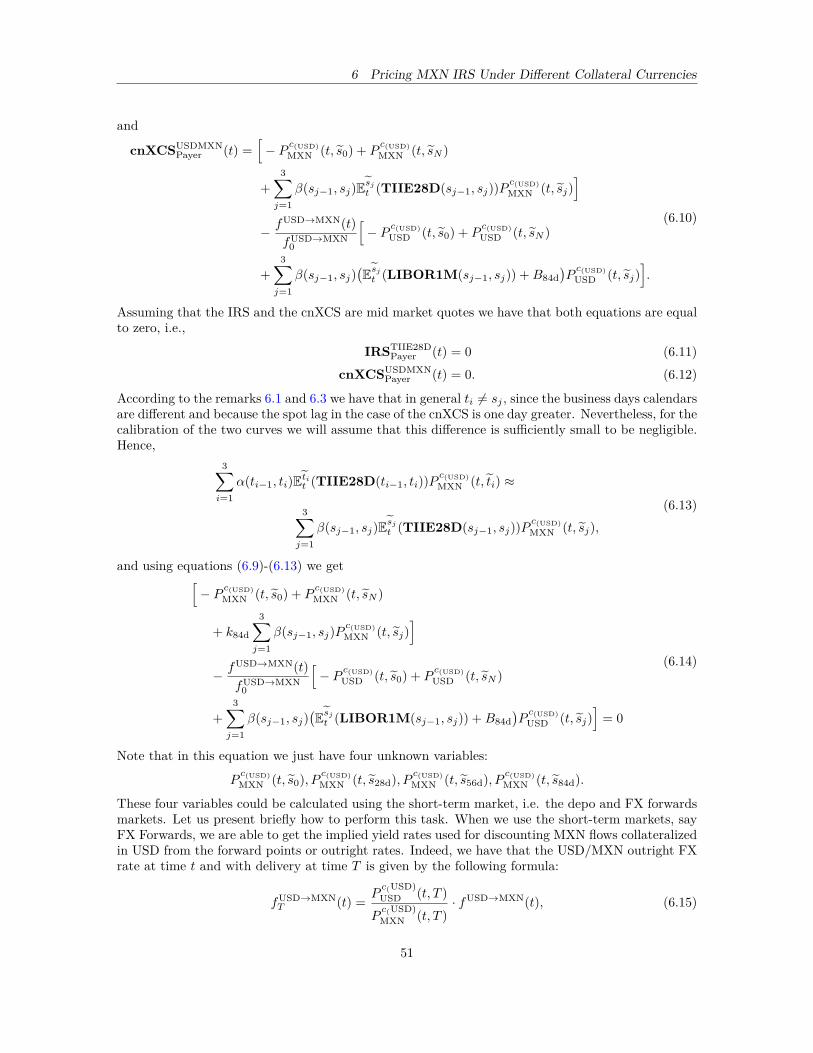
6 Pricing MXN IRS Under Different Collateral Currencies
and
cnXCSUSDMXNPayer (t) =
[− P c(USD)
MXN (t, s0) + Pc(USD)MXN (t, sN )
+3∑j=1
β(sj−1, sj)Esjt (TIIE28D(sj−1, sj))P
c(USD)MXN (t, sj)
]− fUSD→MXN(t)
fUSD→MXN0
[− P c(USD)
USD (t, s0) + Pc(USD)USD (t, sN )
+3∑j=1
β(sj−1, sj)(Esjt (LIBOR1M(sj−1, sj)) +B84d
)Pc(USD)USD (t, sj)
].
(6.10)
Assuming that the IRS and the cnXCS are mid market quotes we have that both equations are equalto zero, i.e.,
IRSTIIE28DPayer (t) = 0 (6.11)
cnXCSUSDMXNPayer (t) = 0. (6.12)
According to the remarks 6.1 and 6.3 we have that in general ti 6= sj , since the business days calendarsare different and because the spot lag in the case of the cnXCS is one day greater. Nevertheless, for thecalibration of the two curves we will assume that this difference is sufficiently small to be negligible.Hence,
3∑i=1
α(ti−1, ti)Etit (TIIE28D(ti−1, ti))Pc(USD)MXN (t, ti) ≈
3∑j=1
β(sj−1, sj)Esjt (TIIE28D(sj−1, sj))P
c(USD)MXN (t, sj),
(6.13)
and using equations (6.9)-(6.13) we get[− P c(USD)
MXN (t, s0) + Pc(USD)MXN (t, sN )
+ k84d
3∑j=1
β(sj−1, sj)Pc(USD)MXN (t, sj)
]− fUSD→MXN(t)
fUSD→MXN0
[− P c(USD)
USD (t, s0) + Pc(USD)USD (t, sN )
+3∑j=1
β(sj−1, sj)(Esjt (LIBOR1M(sj−1, sj)) +B84d
)Pc(USD)USD (t, sj)
]= 0
(6.14)
Note that in this equation we just have four unknown variables:
Pc(USD)MXN (t, s0), P c(USD)
MXN (t, s28d), P c(USD)MXN (t, s56d), P c(USD)
MXN (t, s84d).
These four variables could be calculated using the short-term market, i.e. the depo and FX forwardsmarkets. Let us present briefly how to perform this task. When we use the short-term markets, sayFX Forwards, we are able to get the implied yield rates used for discounting MXN flows collateralizedin USD from the forward points or outright rates. Indeed, we have that the USD/MXN outright FXrate at time t and with delivery at time T is given by the following formula:
fUSD→MXNT (t) = P
c(USD)USD (t, T )Pc(USD)MXN (t, T )
· fUSD→MXN(t), (6.15)
51
6 Pricing MXN IRS Under Different Collateral Currencies
where fUSD→MXN(t) is the FX spot rate. This market is sufficiently liquid to get prices for manytenors, so we are able to get the following outright FX rates:
fUSD→MXNs0
(t), fUSD→MXNs28d
(t), fUSD→MXNs56d
(t), fUSD→MXNs84d
(t).
Hence, using equation (6.15) we can get the values of the discount factors P c(USD)MXN (t, T ) when t ≤ T ≤
1. One obstacle to proceeding with the short-term market method along the rest of the curve is that,even in major currencies (say G7 currencies22), FX forwards are only liquid for two or five years andquoted at most for ten years. For this reason we need long-dated market data (IRS and cnXCS) whichare quoted up to 30 years. In this work we will only use IRSs and cnXCS for the curve calibrationalthough [MexDer, 2014] suggests to use the short-term market for the calibration of the curves upto 1 year and the long-dated swaps for the rest of the curve.
Before we present formally the algorithm of the multiple bootstrapping, let us continue with thecurve calibration when the market only has one IRS and one XCS with maturity of 84 days (threecoupons).
We know that every discount factor has an associated yield rate that holds the following equation:
Pc(USD)MXN (t, x) = e−(x−t)R(t,x). (6.16)
Solving for R(t, x) yields,
R(t, x) = −ln(Pc(USD)MXN (t, x)
)x− t
. (6.17)
In this method the value of P c(USD)MXN (t, s0) is calculated by the short-term method and defines a yield
rate r0 associated to it. For the other three variables P c(USD)MXN (t, s28d), P c(USD)
MXN (t, s56d), P c(USD)MXN (t, s84d)
we need to find a value of R(t, s84d) that satisfy the following conditions:
1. R(t, x) = a+ b(x− t) + c(x− t)2 + d(x− t)3 with s0 ≤ x ≤ s84d and a, b, c, d ∈ R
2. R(t, s0) = r0
3. R(t, x) ∈ C2 with R′′(t, s0) = 0 and R′′(t, s84d) = 0.
These conditions corresponds to the natural cubic splines interpolation method. Note that the aboveconditions defines the next system of equations:
a+ b(s0 − t) + c(s0 − t)2 + d(s0 − t)3 = r0 (6.18)2c+ 6d(s0 − t) = 0 (6.19)
2c+ 6d(s84d − t) = 0. (6.20)
So we get a system of equations with 4 variables and only 3 equations, hence we have two define afourth equation with the intention to get a solution. So we say that
R(t, s84d) := k84d (6.21)=⇒ a+ b(s84d − t) + c(s84d − t)2 + d(s84d − t)3 = k84d (6.22)
In other words, we are claiming that the yield zero coupon rate at time t with maturity in s84d isequal the swap rate for the same tenor. With this new equation the system has a unique solutiongiven by the following vector (a0, b0, c0, d0). We these coefficients we are now able to get the valuesof R0(t, s0), R0(t, s28d), R0(t, s56d), R0(t, s84d) and hence the values of P c(USD)
MXN,0(t, s0), P c(USD)MXN,0(t, s28d),
Pc(USD)MXN,0(t, s56d), P c(USD)
MXN,0(t, s84d). The subscript zero in R0 and P c0 is because we want to emphasize22USD, CAD, GBP, EUR and JPY.
52
6 Pricing MXN IRS Under Different Collateral Currencies
that the values are initial values since we made an initial guess for R0(t, s84d). Note that we are alsoable to calculate the values of R0(t, t0), R0(t, t28d), R0(t, t56d), R0(t, t84d) and substitute them intoequation (6.9). This give us the following equation
IRSTIIE28DPayer (t) =
3∑i=1
α(ti−1, ti)Etit (TIIE28D(ti−1, ti))Pc(USD)MXN (t, ti)
− k84d
3∑i=1
α(ti−1, ti)Pc(USD)MXN (t, ti).
(6.23)
Now the unknown variables in the equation (6.23) are Et56dt (TIIE28D(t28d, t56d)) and Et84d
t (TIIE28D(t56d, t84d)).To find the value of these two variables we are going to make the same assumptions done previouslyi.e. define RTIIE(t, x) yield zero curve that replicates the TIIE 28d forward curve Ext (TIIE28D(x, x+28d)). Likewise, we will assume that RTIIE(t, x) is a piecewise-defined function with the natural cubicsplines conditions. Therefore we have that
1. RTIIE(t, x) = e+ f(x− t) + g(x− t)2 + h(x− t)3 with t0 ≤ x ≤ t84d and e, f, g, h ∈ R,
2. RTIIE(t, y) = TIIE28D(t) for all y ∈ [t0, t28d],
3. RTIIE(t, x) ∈ C2 with R′′(t, t28d) = 0 and R′′(t, t84d) = 0.
Condition 2 states that the function RTIIE has a constant value in the interval [t0, t28d] and this valueis equal to the TIIE 28d reference rate at time t, i.e. equal to the fixing rate published in the tradedate. This assumption guarantees that the forward rate implied from the yield curve RTIIE is theTIIE 28d fixing. Let us present the proof of this (straightforward) fact. We know that the TIIE 28dforward rates are given by the following equation
ETt (TIIE28D(S, T )) = − 1τ(S, T ) ln
(PTIIE(t, S)PTIIE(t, T )
)(6.24)
Now we have that PTIIE(t, x) = e−(x−t)RTIIE(t,x) and RTIIE(t, S) = RTIIE(t, T ) = TIIE28D(t) hence
ETt (TIIE28D(S, T )) = − 1T − S
ln(e−(S−t)TIIE28D(t)
e−(T−t)TIIE28D(t)
)(6.25)
= − ln(e−(T−S)TIIE28D(t))T − S
(6.26)
= TIIE28D(t). (6.27)
Hence, condition 2 guarantees us that the curve replicates the known fixing at time t. Now if we writethe system of equation that can be induced from conditions 1, 2 and 3 we obtain
e+ f(t0 − t) + g(t0 − t)2 + h(t0 − t)3 = TIIE28D(t) (6.28)2g + 6h(t0 − t) = 0 (6.29)
2g + 6h(t84d − t) = 0. (6.30)
Again we have three equations and four variables e, f, g, h so we have to define an equation that allowus to get a solution. So we will say that
RTIIE(t, t84d) := TIIE28D(t) + ε0, ε0 ∈ R (6.31)=⇒ e+ f(t84d − t) + c(t84d − t)2 + d(t84d − t)3 = TIIE28D(t) + ε0 (6.32)
53
6 Pricing MXN IRS Under Different Collateral Currencies
The value of ε0 is a parameter of the rate curve construction that will help us to converge rapidly to asolution. This parameter depends on the structure of the curve and in the monetary policy decisionsthat the central bank could take in the future. For example, if the market is pricing a rate hike inthe following months then we have that ε0 > 0. This parameter is only a variable that serves to easethe convergence of the algorithm. Once we have the coefficient vector (e0, f0, g0, h0) we are able tocalculate the forwards rates of TIIE 28d. Then we substitute these forward rates into equation (6.23)and we generate a mark-to-market Π0
0 for a plain vanilla IRS given by:
Π00(RTIIE
0 (t, s56d), RTIIE0 (t, s84d), ε0) =
3∑i=1
α(ti−1, ti)Etit (TIIE28D(ti−1, ti))Pc(USD)MXN (t, ti)
− k84d
3∑i=1
α(ti−1, ti)Pc(USD)MXN (t, ti).
(6.33)
The value of Π00(RTIIE
0 (t, s56d), RTIIE0 (t, s84d), ε0) is not necessarily equal to zero, so the swap rate
k84d of the IRS is not at par. The idea of this algorithm is to make the mark-to-market Π00 equal
to zero, so we have to find the root of the equation (6.33). In this work we will apply the bisectionmethod for this task although there exists more efficient methods for finding roots such as Newton-Raphson method (see [Burden and Faires, 2010]). Hence, we have to change the value of ε0 and thencalculate the values of (e0, f0, g0, h0) until Π0
0 ≈ 0. Then we substitute the forward rates of TIIE 28dinto the cnXCS equation (6.10). If cnXCSUSDMXN
Payer (t) = 0 then we are done with the iterations ofthe algorithm. However, typically before one iteration we do not have that cnXCSUSDMXN
Payer (t) = 0therefore we have to proceed with more iterations. From equation (6.10) we have to bootstrap thenew coefficients (a1, b1, c1, d1) to make it equal zero. Once we have achieved this task
Πm(Rm(t, s0), Rm(t,s28d), Rm(t, s56d), Rm(t, s84d)) =[− P c(USD)
MXN,m(t, s0) + Pc(USD)MXN,m(t, sN )
+ k84d
3∑j=1
β(sj−1, sj)Pc(USD)MXN,m(t, sj)
]− fUSD→MXN(t)
fUSD→MXN0
[− P c(USD)
USD (t, s0) + Pc(USD)USD (t, sN )
+3∑j=1
β(sj−1, sj)(Esjt (LIBOR1M(sj−1, sj)) +B84d
)Pc(USD)USD (t, sj)
](6.34)
The value of Π0(R0(t, s0), R0(t, s28d), R0(t, s56d), R0(t, s84d)) is in general different to zero since wemade an initial guess for the value of R0(t, s84d). The idea of the multiple bootstrapping is that haveto iterate the values of R0(t, s84d) and make the IRS and cnXCS mark-to-markets equal to zero.
54
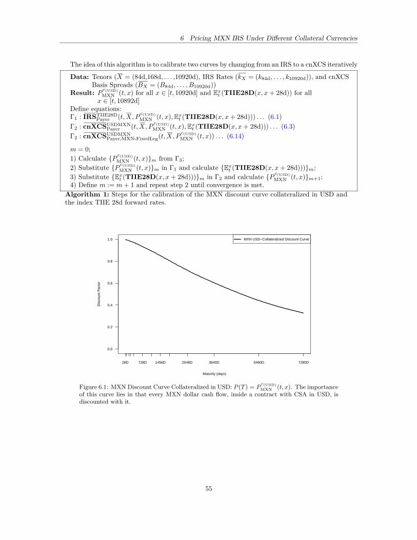
6 Pricing MXN IRS Under Different Collateral Currencies
The idea of this algorithm is to calibrate two curves by changing from an IRS to a cnXCS iteratively
Data: Tenors (X = (84d,168d, . . . ,10920d), IRS Rates (kX = (k84d, . . . , k10920d)), and cnXCSBasis Spreads (BX = (B84d, . . . , B10920d))
Result: P c(USD)MXN (t, x) for all x ∈ [t, 10920d] and Ext (TIIE28D(x, x+ 28d)) for allx ∈ [t, 10892d]
Define equations:Γ1 : IRSTIIE28D
Payer (t,X, P c(USD)MXN (t, x),Ext (TIIE28D(x, x+ 28d))) . . . (6.1)
Γ2 : cnXCSUSDMXNPayer (t,X, P c(USD)
MXN (t, x),Ext (TIIE28D(x, x+ 28d))) . . . (6.3)Γ2 : cnXCSUSDMXN
Payer,MXN-FixedLeg(t,X, P c(USD)MXN (t, x)) . . . (6.14)
m = 0;1) Calculate P c(USD)
MXN (t, x)m from Γ3;2) Substitute P c(USD)
MXN (t, x)m in Γ1 and calculate Ext (TIIE28D(x, x+ 28d)))m;3) Substitute Ext (TIIE28D(x, x+ 28d)))m in Γ2 and calculate P c(USD)
MXN (t, x)m+1;4) Define m := m+ 1 and repeat step 2 until convergence is met.
Algorithm 1: Steps for the calibration of the MXN discount curve collateralized in USD andthe index TIIE 28d forward rates.
0.0
0.2
0.4
0.6
0.8
1.0
Maturity (days)
Dis
coun
t Fac
tor
28D 728D 1456D 2548D 3640D 5460D 7280D
MXN USD−Collateralized Discount Curve
Figure 6.1: MXN Discount Curve Collateralized in USD: P (T ) = Pc(USD)MXN (t, x). The importance
of this curve lies in that every MXN dollar cash flow, inside a contract with CSA in USD, isdiscounted with it.
55
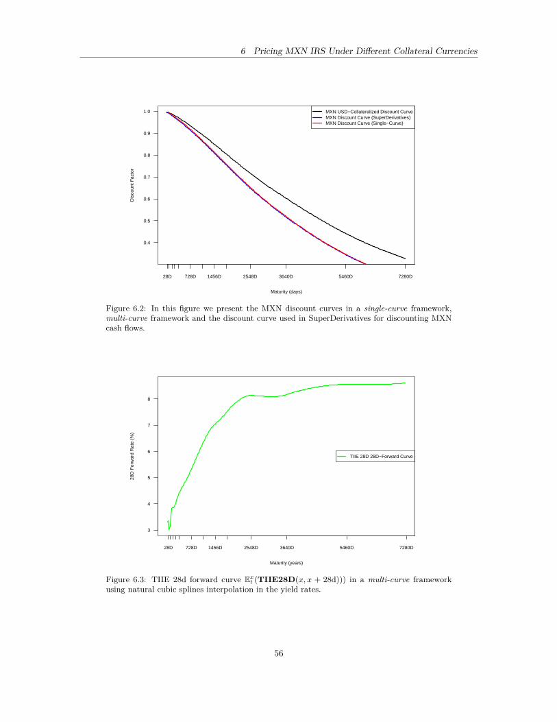
6 Pricing MXN IRS Under Different Collateral Currencies
0.4
0.5
0.6
0.7
0.8
0.9
1.0
Maturity (days)
Dis
coun
t Fac
tor
28D 728D 1456D 2548D 3640D 5460D 7280D
MXN USD−Collateralized Discount CurveMXN Discount Curve (SuperDerivatives)MXN Discount Curve (Single−Curve)
Figure 6.2: In this figure we present the MXN discount curves in a single-curve framework,multi-curve framework and the discount curve used in SuperDerivatives for discounting MXNcash flows.
3
4
5
6
7
8
Maturity (years)
28D
For
war
d R
ate
(%)
28D 728D 1456D 2548D 3640D 5460D 7280D
TIIE 28D 28D−Forward Curve
Figure 6.3: TIIE 28d forward curve Ext (TIIE28D(x, x + 28d))) in a multi-curve framework
using natural cubic splines interpolation in the yield rates.
56
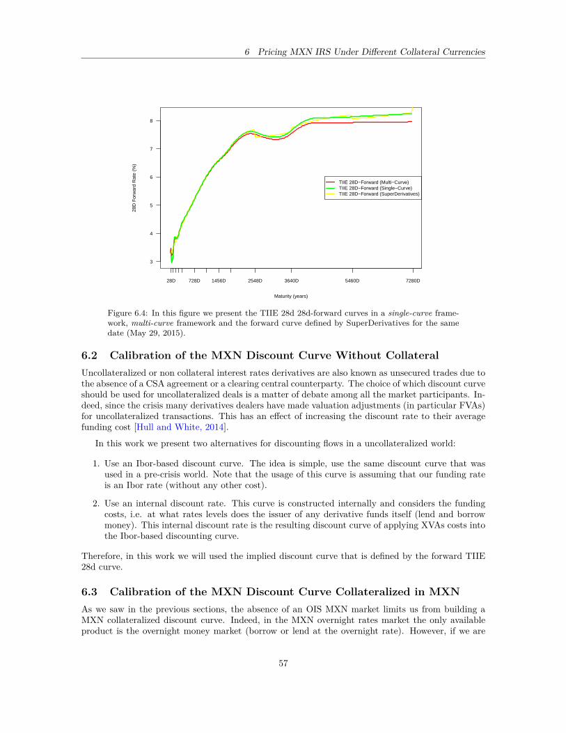
6 Pricing MXN IRS Under Different Collateral Currencies
3
4
5
6
7
8
Maturity (years)
28D
For
war
d R
ate
(%)
28D 728D 1456D 2548D 3640D 5460D 7280D
TIIE 28D−Forward (Multi−Curve)TIIE 28D−Forward (Single−Curve)TIIE 28D−Forward (SuperDerivatives)
Figure 6.4: In this figure we present the TIIE 28d 28d-forward curves in a single-curve frame-work, multi-curve framework and the forward curve defined by SuperDerivatives for the samedate (May 29, 2015).
6.2 Calibration of the MXN Discount Curve Without CollateralUncollateralized or non collateral interest rates derivatives are also known as unsecured trades due tothe absence of a CSA agreement or a clearing central counterparty. The choice of which discount curveshould be used for uncollateralized deals is a matter of debate among all the market participants. In-deed, since the crisis many derivatives dealers have made valuation adjustments (in particular FVAs)for uncollateralized transactions. This has an effect of increasing the discount rate to their averagefunding cost [Hull and White, 2014].
In this work we present two alternatives for discounting flows in a uncollateralized world:
1. Use an Ibor-based discount curve. The idea is simple, use the same discount curve that wasused in a pre-crisis world. Note that the usage of this curve is assuming that our funding rateis an Ibor rate (without any other cost).
2. Use an internal discount rate. This curve is constructed internally and considers the fundingcosts, i.e. at what rates levels does the issuer of any derivative funds itself (lend and borrowmoney). This internal discount rate is the resulting discount curve of applying XVAs costs intothe Ibor-based discounting curve.
Therefore, in this work we will used the implied discount curve that is defined by the forward TIIE28d curve.
6.3 Calibration of the MXN Discount Curve Collateralized in MXNAs we saw in the previous sections, the absence of an OIS MXN market limits us from building aMXN collateralized discount curve. Indeed, in the MXN overnight rates market the only availableproduct is the overnight money market (borrow or lend at the overnight rate). However, if we are
57
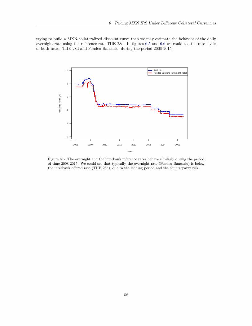
6 Pricing MXN IRS Under Different Collateral Currencies
trying to build a MXN-collateralized discount curve then we may estimate the behavior of the dailyovernight rate using the reference rate TIIE 28d. In figures 6.5 and 6.6 we could see the rate levelsof both rates: TIIE 28d and Fondeo Bancario, during the period 2008-2015.
0
2
4
6
8
10
Year
Pub
lishe
d R
ates
(%
)
2008 2009 2010 2011 2012 2013 2014 2015
TIIE 28dFondeo Bancario (Overnight Rate)
Figure 6.5: The overnight and the interbank reference rates behave similarly during the periodof time 2008-2015. We could see that typically the overnight rate (Fondeo Bancario) is belowthe interbank offered rate (TIIE 28d), due to the lending period and the counterparty risk.
58
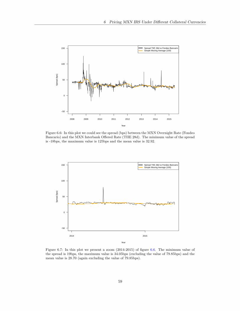
6 Pricing MXN IRS Under Different Collateral Currencies
−50
0
50
100
150
Year
Spr
ead
(bps
)
2008 2009 2010 2011 2012 2013 2014 2015
Spread TIIE 28d vs Fondeo BancarioSimple Moving Average (100)
Figure 6.6: In this plot we could see the spread (bps) between the MXN Overnight Rate (FondeoBancario) and the MXN Interbank Offered Rate (TIIE 28d). The minimum value of the spreadis -18bps, the maximum value is 125bps and the mean value is 32.92.
−50
0
50
100
150
Year
Spr
ead
(bps
)
2014 2015
Spread TIIE 28d vs Fondeo BancarioSimple Moving Average (100)
Figure 6.7: In this plot we present a zoom (2014-2015) of figure 6.6. The minimum value ofthe spread is 19bps, the maximum value is 34.05bps (excluding the value of 79.85bps) and themean value is 28.70 (again excluding the value of 79.85bps).
59
6 Pricing MXN IRS Under Different Collateral Currencies
Hence it is valid to assume that:
Overnight Rate in MXN = TIIE 28d− 29bps (6.35)
Using the forward curve of TIIE 28d calibrated in section 6.1 and equation (6.35) we can calculatethe daily overnight rates (forward rates). Then it is quite simple to calculate the implied yield curveand hence we obtain the MXN-collateralized discount curve.
Remark 6.5. It is important to point out that the assumption of equation (6.35) could be dangeroussince the spread between TIIE 28d and Fondeo Bancario can widen or reduce suddenly. Furthermore,we are unable to hedge this spread with interest rate products, hence pricing these MXN-collateralizedIRSs with the assumption of constant difference between TIIE 28d and Fondeo Bancario is risky.
6.4 Calibration of the MXN Discount Curve Collateralized in EURThe arguments for the construction of the MXN discount curve collateralized in EUR can be usedfor almost every currency in the world. Indeed, if we are able to build the discount curve for USDcash flows collateralized in a currency ABC, then by no-arbitrage arguments we could build the MXNdiscount curve collateralized in ABC.
Let us explain the arguments for the construction of the MXN discount curve collateralized inEUR. According to the flowchart in figure 5.9, we know that using the EURUSD mtmXCSs we get—directly with a simple bootstrapping— the curve P c(EUR)
USD (t, x), since the market quotes are collat-eralized in EUR. In fact, in section 5.3.1 we exhibit the steps to follow for the calibration of thiscurve.
Proposition 6.1. The discount curve for MXN cash flows collateralized in EUR is given by thefollowing formula:
Pc(EUR)MXN (t, x) = P
c(EUR)USD (t, x)P c(USD)
MXN (t, x)Pc(USD)USD (t, x)
. (6.36)
Proof. Let P c(EUR)MXN (t, T ) be the T -maturity MXN zero coupon bond fully-collateralized in EUR. In
other words, P c(EUR)MXN (t, T ) is the present value of MXN$1 at time T . Then, if we buy the zero coupon
bond we have the following cash flows:
Time Cash Flow (MXN)t −P
c(EUR)MXN (t, T )
T +1
Now we have to build a trading strategy that replicates the previous cash flows. Suppose that webuy USD$X units of a T -maturity USD zero coupon bond fully-collateralized in EUR. Hence we havethe following cash flows:
Time Cash Flow (USD)t −XP
c(EUR)USD (t, T )
T +X
Note that these last cash flows are denominated in USD currency. Then we could enter into a FXSwap (mid market quote) that allow us to exchange the USD cash flow at time T for cahs flows inMXN currency. Therefore, using the spot and forward rates we have the following MXN cash flows:
60
6 Pricing MXN IRS Under Different Collateral Currencies
Time Cash Flow (MXN)t −StXP
c(EUR)USD (t, T )
T +ST X
where St is the spot FX rate and ST is the forward FX rate. For USD-collateralized FX forwards weknow that,
ST = StPc(USD)USD (t, T )Pc(USD)MXN (t, T )
. (6.37)
Now, let us define X as
X := Pc(USD)MXN (t, T )
StPc(USD)USD (t, T )
.
If we substitute X into the MXN cash flows of the replication trading strategy we have that:
Time Cash Flow (MXN)
t −Pc(USD)MXN (t,T )P
c(EUR)USD (t,T )
Pc(USD)USD (t,T )
T +1
This bring us a trading strategy that give us the same cash flow of MXN$1 at maturity T whenthe collateral currency is EUR. Hence, by no-arbitrage arguments,
Pc(EUR)MXN (t, T ) = P
c(EUR)USD (t, T )P c(USD)
MXN (t, x)Pc(USD)USD (t, T )
.
As we mention earlier, this proposition can be reproduced for other currencies such as: CAD, JPY,GBP, CHF, BRL, etc. For the construction of the curve, We just need the discounting curve of USDcash flows collateralized in the other currency. The next proposition generalizes the previous case ofEUR currency as collateral.
Proposition 6.2. The discount curve for MXN cash flows collateralized in ABC is given by thefollowing formula:
Pc(ABC)MXN (t, x) = P
c(ABC)USD (t, x)P c(USD)
MXN (t, x)Pc(USD)USD (t, x)
, (6.38)
where ABC denotes any currency code ISO 4217.
Proof. See the proof of proposition 6.1.
61
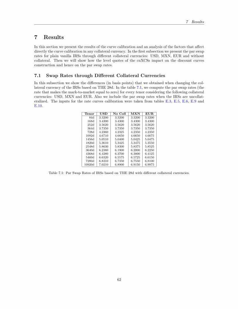
7 Results
7 ResultsIn this section we present the results of the curve calibration and an analysis of the factors that affectdirectly the curve calibration in any collateral currency. In the first subsection we present the par swaprates for plain vanilla IRSs through different collateral currencies: USD, MXN, EUR and withoutcollateral. Then we will show how the level quotes of the cnXCSs impact on the discount curvesconstruction and hence on the par swap rates.
7.1 Swap Rates through Different Collateral CurrenciesIn this subsection we show the differences (in basis points) that we obtained when changing the col-lateral currency of the IRSs based on TIIE 28d. In the table 7.1, we compute the par swap rates (therate that makes the mark-to-market equal to zero) for every tenor considering the following collateralcurrencies: USD, MXN and EUR. Also we include the par swap rates when the IRSs are uncollat-eralized. The inputs for the rate curves calibration were taken from tables E.3, E.5, E.6, E.9 andE.10.
Tenor USD No Coll MXN EUR84d 3.3200 3.3200 3.3200 3.3200168d 3.4300 3.4300 3.4300 3.4300252d 3.5620 3.5620 3.5620 3.5620364d 3.7350 3.7350 3.7350 3.7350728d 4.2360 4.2325 4.2350 4.23501092d 4.6710 4.6650 4.6650 4.66751456d 5.0510 5.0400 5.0425 5.04751820d 5.3610 5.3425 5.3475 5.35502548d 5.8630 5.8300 5.8375 5.85253640d 6.2380 6.1900 6.2000 6.22504368d 6.4280 6.3700 6.3800 6.41255460d 6.6320 6.5575 6.5725 6.61507280d 6.8310 6.7350 6.7550 6.810010920d 7.0210 6.8900 6.9150 6.9975
Table 7.1: Par Swap Rates of IRSs based on TIIE 28d with different collateral currencies.
62
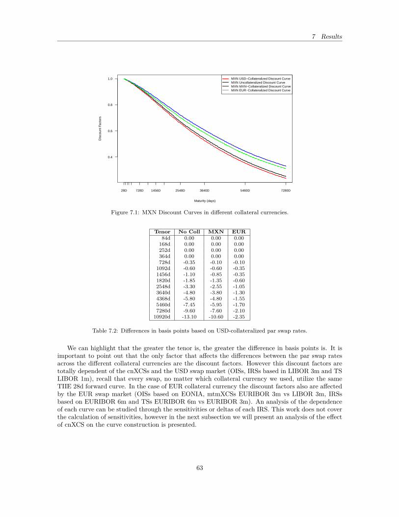
7 Results
0.4
0.6
0.8
1.0
Maturity (days)
Dis
coun
t Fac
tors
28D 728D 1456D 2548D 3640D 5460D 7280D
MXN USD−Collateralized Discount CurveMXN Uncollateralized Discount CurveMXN MXN−Collateralized Discount CurveMXN EUR−Collateralized Discount Curve
Figure 7.1: MXN Discount Curves in different collateral currencies.
Tenor No Coll MXN EUR84d 0.00 0.00 0.00168d 0.00 0.00 0.00252d 0.00 0.00 0.00364d 0.00 0.00 0.00728d -0.35 -0.10 -0.101092d -0.60 -0.60 -0.351456d -1.10 -0.85 -0.351820d -1.85 -1.35 -0.602548d -3.30 -2.55 -1.053640d -4.80 -3.80 -1.304368d -5.80 -4.80 -1.555460d -7.45 -5.95 -1.707280d -9.60 -7.60 -2.1010920d -13.10 -10.60 -2.35
Table 7.2: Differences in basis points based on USD-collateralized par swap rates.
We can highlight that the greater the tenor is, the greater the difference in basis points is. It isimportant to point out that the only factor that affects the differences between the par swap ratesacross the different collateral currencies are the discount factors. However this discount factors aretotally dependent of the cnXCSs and the USD swap market (OISs, IRSs based in LIBOR 3m and TSLIBOR 1m), recall that every swap, no matter which collateral currency we used, utilize the sameTIIE 28d forward curve. In the case of EUR collateral currency the discount factors also are affectedby the EUR swap market (OISs based on EONIA, mtmXCSs EURIBOR 3m vs LIBOR 3m, IRSsbased on EURIBOR 6m and TSs EURIBOR 6m vs EURIBOR 3m). An analysis of the dependenceof each curve can be studied through the sensitivities or deltas of each IRS. This work does not coverthe calculation of sensitivities, however in the next subsection we will present an analysis of the effectof cnXCS on the curve construction is presented.
63
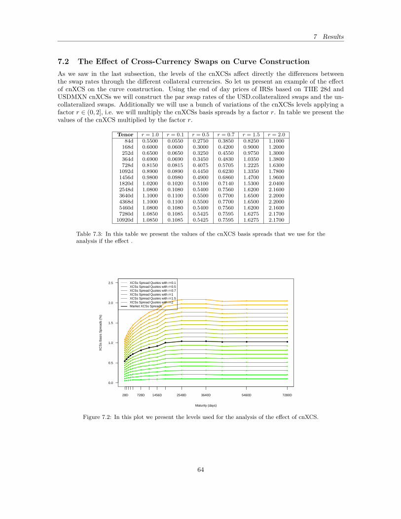
7 Results
7.2 The Effect of Cross-Currency Swaps on Curve ConstructionAs we saw in the last subsection, the levels of the cnXCSs affect directly the differences betweenthe swap rates through the different collateral currencies. So let us present an example of the effectof cnXCS on the curve construction. Using the end of day prices of IRSs based on TIIE 28d andUSDMXN cnXCSs we will construct the par swap rates of the USD.collateralized swaps and the un-collateralized swaps. Additionally we will use a bunch of variations of the cnXCSs levels applying afactor r ∈ (0, 2], i.e. we will multiply the cnXCSs basis spreads by a factor r. In table we present thevalues of the cnXCS multiplied by the factor r.
Tenor r = 1.0 r = 0.1 r = 0.5 r = 0.7 r = 1.5 r = 2.084d 0.5500 0.0550 0.2750 0.3850 0.8250 1.1000168d 0.6000 0.0600 0.3000 0.4200 0.9000 1.2000252d 0.6500 0.0650 0.3250 0.4550 0.9750 1.3000364d 0.6900 0.0690 0.3450 0.4830 1.0350 1.3800728d 0.8150 0.0815 0.4075 0.5705 1.2225 1.63001092d 0.8900 0.0890 0.4450 0.6230 1.3350 1.78001456d 0.9800 0.0980 0.4900 0.6860 1.4700 1.96001820d 1.0200 0.1020 0.5100 0.7140 1.5300 2.04002548d 1.0800 0.1080 0.5400 0.7560 1.6200 2.16003640d 1.1000 0.1100 0.5500 0.7700 1.6500 2.20004368d 1.1000 0.1100 0.5500 0.7700 1.6500 2.20005460d 1.0800 0.1080 0.5400 0.7560 1.6200 2.16007280d 1.0850 0.1085 0.5425 0.7595 1.6275 2.170010920d 1.0850 0.1085 0.5425 0.7595 1.6275 2.1700
Table 7.3: In this table we present the values of the cnXCS basis spreads that we use for theanalysis if the effect .
0.0
0.5
1.0
1.5
2.0
2.5
Maturity (days)
XC
Ss
Bas
is S
prea
ds (
%)
28D 728D 1456D 2548D 3640D 5460D 7280D
XCSs Spread Quotes with r=0.1XCSs Spread Quotes with r=0.5XCSs Spread Quotes with r=0.7XCSs Spread Quotes with r=1XCSs Spread Quotes with r=1.5XCSs Spread Quotes with r=2Market XCSs Spreads
Figure 7.2: In this plot we present the levels used for the analysis of the effect of cnXCS.
64
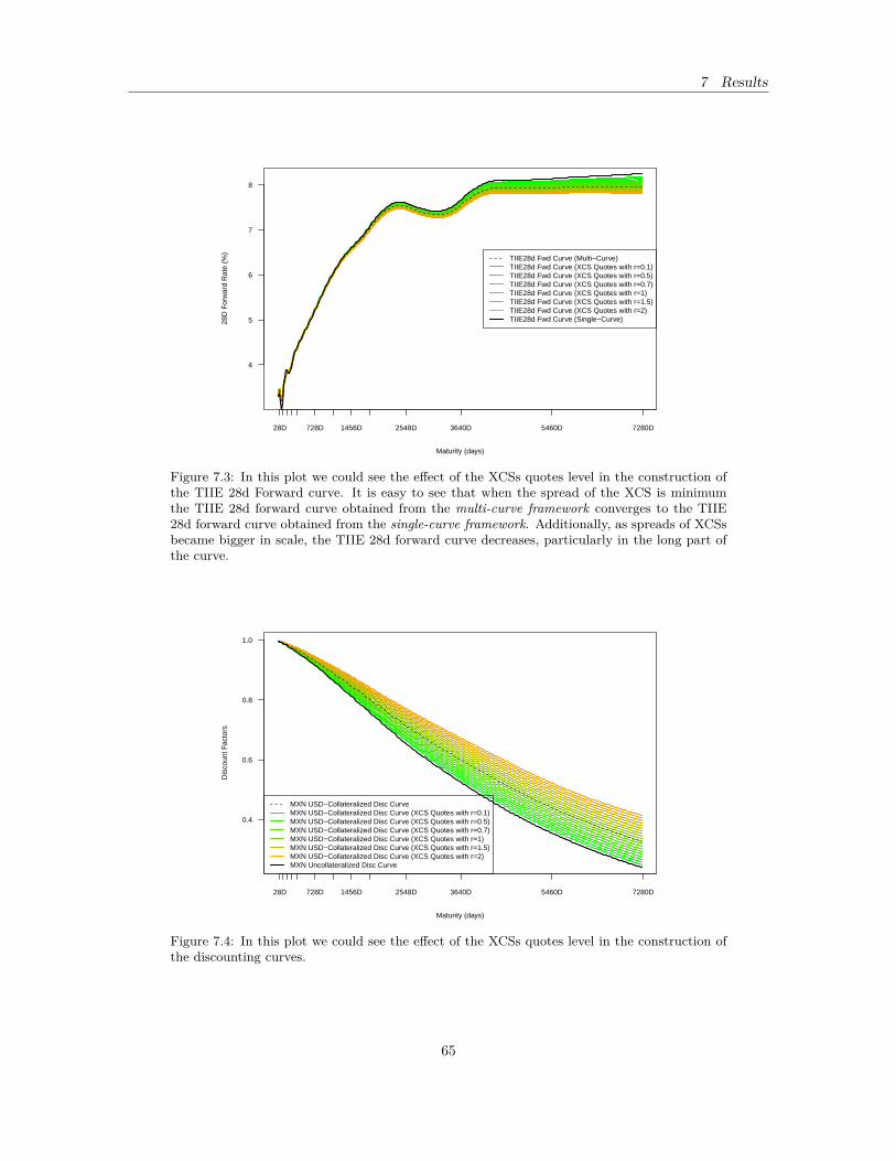
7 Results
4
5
6
7
8
Maturity (days)
28D
For
war
d R
ate
(%)
28D 728D 1456D 2548D 3640D 5460D 7280D
TIIE28d Fwd Curve (Multi−Curve)TIIE28d Fwd Curve (XCS Quotes with r=0.1)TIIE28d Fwd Curve (XCS Quotes with r=0.5)TIIE28d Fwd Curve (XCS Quotes with r=0.7)TIIE28d Fwd Curve (XCS Quotes with r=1)TIIE28d Fwd Curve (XCS Quotes with r=1.5)TIIE28d Fwd Curve (XCS Quotes with r=2)TIIE28d Fwd Curve (Single−Curve)
Figure 7.3: In this plot we could see the effect of the XCSs quotes level in the construction ofthe TIIE 28d Forward curve. It is easy to see that when the spread of the XCS is minimumthe TIIE 28d forward curve obtained from the multi-curve framework converges to the TIIE28d forward curve obtained from the single-curve framework. Additionally, as spreads of XCSsbecame bigger in scale, the TIIE 28d forward curve decreases, particularly in the long part ofthe curve.
0.4
0.6
0.8
1.0
Maturity (days)
Dis
coun
t Fac
tors
28D 728D 1456D 2548D 3640D 5460D 7280D
MXN USD−Collateralized Disc CurveMXN USD−Collateralized Disc Curve (XCS Quotes with r=0.1)MXN USD−Collateralized Disc Curve (XCS Quotes with r=0.5)MXN USD−Collateralized Disc Curve (XCS Quotes with r=0.7)MXN USD−Collateralized Disc Curve (XCS Quotes with r=1)MXN USD−Collateralized Disc Curve (XCS Quotes with r=1.5)MXN USD−Collateralized Disc Curve (XCS Quotes with r=2)MXN Uncollateralized Disc Curve
Figure 7.4: In this plot we could see the effect of the XCSs quotes level in the construction ofthe discounting curves.
65
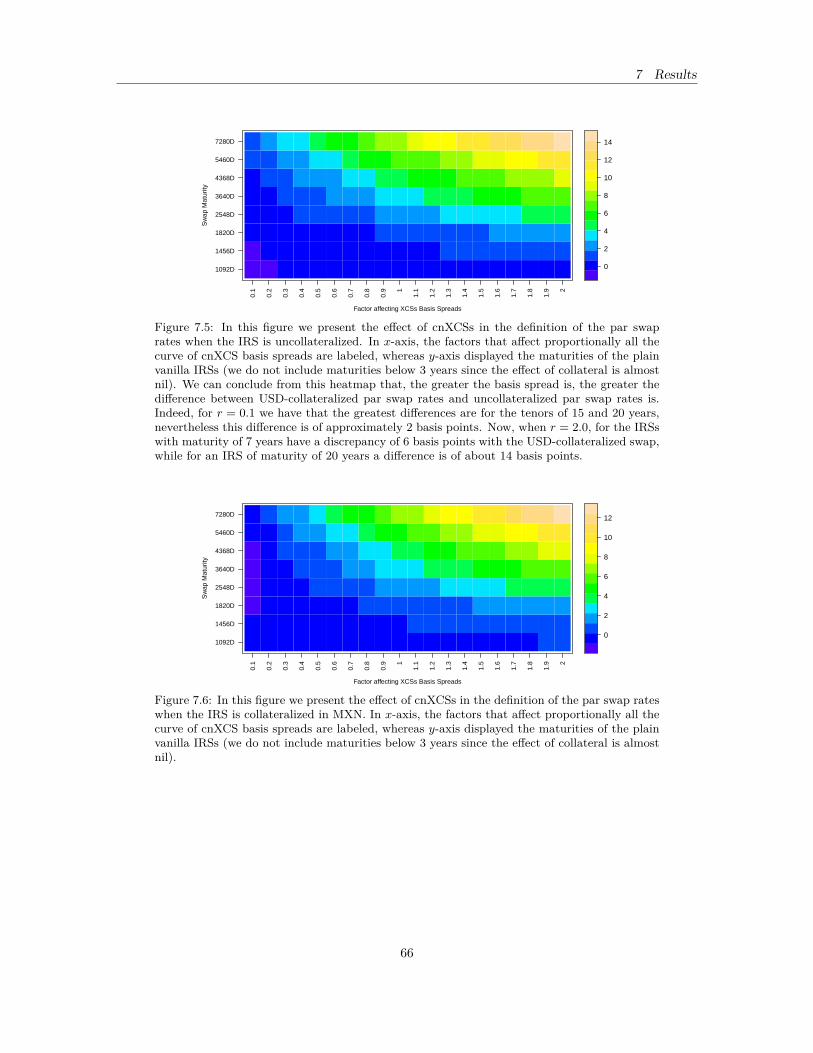
7 Results
Factor affecting XCSs Basis Spreads
Sw
ap M
atur
ity
1092D
1456D
1820D
2548D
3640D
4368D
5460D
7280D
0.1
0.2
0.3
0.4
0.5
0.6
0.7
0.8
0.9 1
1.1
1.2
1.3
1.4
1.5
1.6
1.7
1.8
1.9 2
0
2
4
6
8
10
12
14
Figure 7.5: In this figure we present the effect of cnXCSs in the definition of the par swaprates when the IRS is uncollateralized. In x-axis, the factors that affect proportionally all thecurve of cnXCS basis spreads are labeled, whereas y-axis displayed the maturities of the plainvanilla IRSs (we do not include maturities below 3 years since the effect of collateral is almostnil). We can conclude from this heatmap that, the greater the basis spread is, the greater thedifference between USD-collateralized par swap rates and uncollateralized par swap rates is.Indeed, for r = 0.1 we have that the greatest differences are for the tenors of 15 and 20 years,nevertheless this difference is of approximately 2 basis points. Now, when r = 2.0, for the IRSswith maturity of 7 years have a discrepancy of 6 basis points with the USD-collateralized swap,while for an IRS of maturity of 20 years a difference is of about 14 basis points.
Factor affecting XCSs Basis Spreads
Sw
ap M
atur
ity
1092D
1456D
1820D
2548D
3640D
4368D
5460D
7280D
0.1
0.2
0.3
0.4
0.5
0.6
0.7
0.8
0.9 1
1.1
1.2
1.3
1.4
1.5
1.6
1.7
1.8
1.9 2
0
2
4
6
8
10
12
Figure 7.6: In this figure we present the effect of cnXCSs in the definition of the par swap rateswhen the IRS is collateralized in MXN. In x-axis, the factors that affect proportionally all thecurve of cnXCS basis spreads are labeled, whereas y-axis displayed the maturities of the plainvanilla IRSs (we do not include maturities below 3 years since the effect of collateral is almostnil).
66
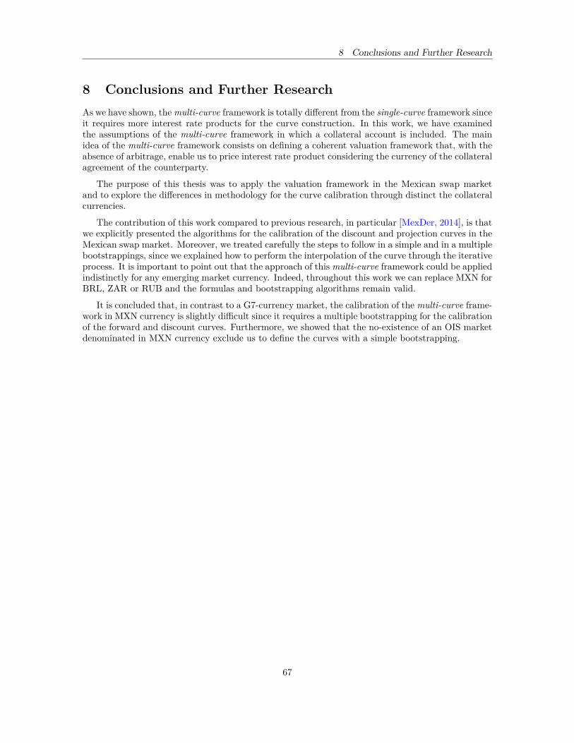
8 Conclusions and Further Research
8 Conclusions and Further ResearchAs we have shown, themulti-curve framework is totally different from the single-curve framework sinceit requires more interest rate products for the curve construction. In this work, we have examinedthe assumptions of the multi-curve framework in which a collateral account is included. The mainidea of the multi-curve framework consists on defining a coherent valuation framework that, with theabsence of arbitrage, enable us to price interest rate product considering the currency of the collateralagreement of the counterparty.
The purpose of this thesis was to apply the valuation framework in the Mexican swap marketand to explore the differences in methodology for the curve calibration through distinct the collateralcurrencies.
The contribution of this work compared to previous research, in particular [MexDer, 2014], is thatwe explicitly presented the algorithms for the calibration of the discount and projection curves in theMexican swap market. Moreover, we treated carefully the steps to follow in a simple and in a multiplebootstrappings, since we explained how to perform the interpolation of the curve through the iterativeprocess. It is important to point out that the approach of this multi-curve framework could be appliedindistinctly for any emerging market currency. Indeed, throughout this work we can replace MXN forBRL, ZAR or RUB and the formulas and bootstrapping algorithms remain valid.
It is concluded that, in contrast to a G7-currency market, the calibration of the multi-curve frame-work in MXN currency is slightly difficult since it requires a multiple bootstrapping for the calibrationof the forward and discount curves. Furthermore, we showed that the no-existence of an OIS marketdenominated in MXN currency exclude us to define the curves with a simple bootstrapping.
67
References
References[Ametrano and Bianchetti, 2013] Ametrano, F. M. and Bianchetti, M. (2013). Everything You Al-
ways Wanted To Know About Multiple Interest Rate Curve Bootstrapping But Were Afraid ToAsk. Available at SSRN 2219548.
[Arteta and Stocker, 2015] Arteta, C. and Stocker, M. (2015). Negative Interest Rates in Europe: AGlance at Their Causes and Implications.
[Bianchetti, 2008] Bianchetti, M. (2008). Two Curves, One Price: Pricing & Hedging Interest RateDerivatives Decoupling Forwarding and Discounting Yield Curves. One Price: Pricing & HedgingInterest Rate Derivatives Decoupling Forwarding and Discounting Yield Curves (November 14,2008).
[Bianchetti and Carlicchi, 2012] Bianchetti, M. and Carlicchi, M. (2012). Markets evolution after thecredit crunch. Available at SSRN 2190138.
[Bicksler and Chen, 1986] Bicksler, J. and Chen, A. H. (1986). An economic analysis of interest rateswaps. The Journal of Finance, 41(3):645–655.
[Black and Scholes, 1973] Black, F. and Scholes, M. (1973). The Pricing of Options and CorporateLiabilities. The Journal of Political Economy, pages 637–654.
[Brigo and Mercurio, 2007] Brigo, D. and Mercurio, F. (2007). Interest Rate Models - Theory andPractice: With Smile, Inflation and Credit. Springer Finance. Springer Berlin Heidelberg.
[Burden and Faires, 2010] Burden, R. and Faires, J. (2010). Numerical Analysis. Cengage Learning.
[Clarke, 2010] Clarke, J. (2010*). Constructing the OIS Curve. Edu-Risk International.
[CME, 2016] CME (2016). Chicago Mercantile Exchange Product Scope: Cleared OTC Interest RateSwaps. http://www.cmegroup.com/trading/interest-rates/cleared-otc/. Accessed: 11 Apr2016.
[Cox et al., 1979] Cox, J., Ross, S., and Rubinstein, M. (1979). Option pricing: A simplified approach.Journal of Financial Economics, 7(3):229–263.
[Du Preez, 2011] Du Preez, P. F. (2011). An investigation into popular methods for constructingyield curves. Master’s thesis, University of Pretoria.
[Fujii et al., 2010a] Fujii, M., Shimada, Y., and Takahashi, A. (2010a). Collateral Posting and Choiceof Collateral Currency. Available at ssrn. com.
[Fujii et al., 2010b] Fujii, M., Shimada, Y., and Takahashi, A. (2010b). A Note on Construction ofMultiple Swap Curves with and without Collateral. FSA Research Review, 6(139-157).
[Fujii et al., 2011] Fujii, M., Shimada, Y., and Takahashi, A. (2011). A market model of interestrates with dynamic basis spreads in the presence of collateral and multiple currencies. Wilmott,2011(54):61–73.
[Fujii and Takahashi, 2015a] Fujii, M. and Takahashi, A. (2015a). Choice of collateral currencyupdated–a market model for the benchmark pricing–. Available at SSRN 2650263.
[Fujii and Takahashi, 2015b] Fujii, M. and Takahashi, A. (2015b). A General Framework for theBenchmark pricing in a Fully Collateralized Market. arXiv preprint arXiv:1508.06339.
68
References
[Green, 2015] Green, A. (2015). XVA: Credit, Funding and Capital Valuation Adjustments. JohnWiley & Sons.
[Gregory, 2012] Gregory, J. (2012). Counterparty Credit Risk and Credit Value Adjustment: A Con-tinuing Challenge for Global Financial Markets. The Wiley Finance Series. Wiley.
[Gunnarsson, 2013] Gunnarsson, S. (2013). Curve Building and Swap Pricing in the Presence of Col-lateral and Basis Spreads. Master’s thesis, Royal Institute of Technology, Sweden.
[Hagan and West, 2006] Hagan, P. S. and West, G. (2006). Interpolation methods for curve construc-tion. Applied Mathematical Finance, 13(2):89–129.
[Hagan and West, 2008] Hagan, P. S. and West, G. (2008). Methods for constructing a yield curve.Wilmott Magazine, May 2008, pages 70–81.
[Hannoun, 2015] Hannoun, H. (2015). Ultra-low or negative interest rates: what they mean for fi-nancial stability and growth. In Remarks by Hervé Hannoun, Deputy General Manager, Bank forInternational Settlements, at the Eurofi High-Level Seminar, Riga, April, volume 22.
[Henrard, 2007] Henrard, M. (2007). The irony in the derivatives discounting. Available at SSRN970509.
[Henrard, 2010] Henrard, M. (2010). The Irony in Derivatives Discounting Part II: The Crisis.Wilmott Journal, 2(6):301–316.
[Henrard, 2012] Henrard, M. (2012). Interest Rate Instruments and Market Conventions Guide.OpenGamma Quantitative Research,.
[Henrard, 2014] Henrard, M. (2014). Interest Rate Modelling in the Multi-Curve Framework. Pal-grave Macmillan.
[Hens and Rieger, 2010] Hens, T. and Rieger, M. O. (2010). Financial economics: A concise intro-duction to classical and behavioral finance. Springer Science & Business Media.
[Hull, 1997] Hull, J. (1997). Options, Futures, and Other Derivatives. Options, Futures, and OtherDerivatives. Prentice Hall.
[Hull and White, 2014] Hull, J. and White, A. (2014). Valuing derivatives: Funding value adjust-ments and fair value. Financial Analysts Journal, 70(3):46–56.
[Ingersoll, 1977] Ingersoll, J. E. (1977). A contingent-claims valuation of convertible securities. Jour-nal of Financial Economics, 4(3):289–321.
[ISDA, 2009] ISDA, D. M. (2009). Alternative compounding methods for over-the-counter derivativetransactions. http://http://www.isda.org/c_and_a/pdf/ISDA-Compounding-memo.pdf. Ac-cessed: 15 Apr 2016.
[Jackson et al., 2015] Jackson, H. et al. (2015). The International Experience with Negative PolicyRates. Bank of Canada Staff Discussion Paper, (2015-13).
[Kuttner, 2001] Kuttner, K. N. (2001). Monetary policy surprises and interest rates: Evidence fromthe fed funds futures market. Journal of monetary economics, 47(3):523–544.
[Labuszewski and Newman, 2014] Labuszewski, J. W. and Newman, A. (2014). Fed Funds Futuresas a Predictive Tool.
69
References
[Lichters et al., 2015] Lichters, R., Stamm, R., and Gallagher, D. (2015). Modern Derivatives Pricingand Credit Exposure Analysis: Theory and Practice of CSA and XVA Pricing, Exposure Simulationand Backtesting. Springer.
[Lidholm and Nudel, 2014] Lidholm, E. and Nudel, B. (2014). Implications of Multiple Curve Con-struction in the Swedish Swap Market.
[Merton, 1973] Merton, R. (1973). Theory of rational option pricing. The Bell Journal of Economicsand Management Science, pages 141–183.
[MexDer, 2014] MexDer (2014). Análisis Comparativo de las Metodologías de Valuación de Swapsde TIIE. Mercado Mexicano de Derivados.
[Miron and Swannell, 1991] Miron, P. and Swannell, P. (1991). Pricing and hedging swaps. Eu-romoney Publ.
[Pallavicini and Tarenghi, 2010] Pallavicini, A. and Tarenghi, M. (2010). Interest-rate Modeling withMultiple Yield Curves. Available at SSRN 1629688.
[Piterbarg, 2010] Piterbarg, V. (2010). Funding beyond discounting: collateral agreements andderivatives pricing. Risk, 23(2):97.
[Piterbarg, 2012] Piterbarg, V. (2012). Cooking with collateral. Risk, 25(8):46.
[Robertson et al., 1997] Robertson, J. C., Thornton, D. L., et al. (1997). Using federal funds futuresrates to predict Federal Reserve actions. Review-Federal Reserve Bank of Saint Louis, 79:45–53.
[Ron et al., 2000] Ron, U. et al. (2000). A practical guide to swap curve construction. Bank of CanadaOttawa.
[Ruiz, 2015] Ruiz, I. (2015). XVA Desks-a New Era for Risk Management: Understanding, Buildingand Managing Counterparty, Funding and Capital Risk. Springer.
[Sengupta et al., 2008] Sengupta, R., Tam, Y. M., et al. (2008). The LIBOR-OIS Spread as a Sum-mary Indicator. Monetary Trends, (Nov).
[Spoor, 2013] Spoor, J. (2013). Double Effect: Multiple Interest Rate Curve Bootstrapping. Master’sthesis, University of Twente.
[Takada, 2011] Takada, K. K. (2011). Valuation of Arithmetic Average of Fed Funds Rates and Con-struction of the US dollar Swap Yield Curve. Available at SSRN 1981668.
70
A Proofs
A Proofs
A.1 Proof of Theorem 5.3Proof. Let us say that the forward measure Tαc has associated the numéraire Pαc(t, T ). This numérairecorresponds to the price of the partially collateralized (α) zero coupon bond. Using theorem 5.2 andthe risk neutral measure Q with the numéraire X(t) := exp(−
∫ Tt
(1−α)r(s) +αc(s)ds) we have that
ζα(t) = EQt
(dTαc
dQ
)= P c(t, T )X(0)P c(0, T )X(t) . (A.1)
Using equation (5.9) and theorem 5.1 we get that
h(t) = EQt
[e−∫ Tt
(1−α)r(s)+αc(s)dsh(T )
]= EQ
t [X(t)h(T )]
= EQt
[Pαc(t, T )ζα(T )
ζα(t) h(T )]
= ζ−1α (t)EQ
t [ζα(T )Pαc(t, T )h(T )]= ETαc
t [Pαc(t, T )h(T )]= Pαc(t, T )ETαc
t [h(T )] .
71
B Conventions & Calendars
B Conventions & CalendarsIn this appendix, we will define the conventions and calendars used within the work. For a morecomplete detailed information of the conventions and calendars throughout the different interest ratesmarkets around world, see [Henrard, 2012].
B.1 Day Count ConventionsACT/360: The year fraction between two dates is computed by dividing the actual days betweentwo dates by 360, i.e.,
Year Fraction = Actual Days360 . (B.1)
ACT/365: The year fraction between two dates is computed by dividing the actual days betweentwo dates by 365, i.e.,
Year Fraction = Actual Days360 . (B.2)
ACT/ACT (ISDA): The year fraction is computed by making difference between days in a leapyear and days in a non-leap year, i.e.,
Year Fraction = Days in a leap year366 + Days in a non-leap year
365 . (B.3)
30/360: The year fraction is computed by assuming that months have 30 days and years have 360,i.e.,
Year Fraction = 360 · (Y2 − Y1) + 30 · (M2 −M1) + (D2 −D1)360 . (B.4)
B.2 Date Rolling ConventionsFollowing: If a payment date falls on a non-business day, the payment date is set to the next businessday.Example: Start date: 30-Oct-2014 with a period 1 month → End date: 01-Dec-2014
Modified Following: If a payment date falls on a non-business day, the payment date is set to thenext business day with the exception that if the next business day falls in a new month then thepayment date is set to the last business day.Example: Start date: 30-Oct-2014 with a period 1 month → End date: 28-Nov-2014
B.3 CalendarsIn this work we used MX, US and UK calendars. The difference among them relies on the holidaysasumed by each central bank or the responsible for determining the fixings of certain rates. Belowyou will find the holidays of each region.
MX (Mexico): New Year’s Day, Constitution Day, Birth Anniversary of Benito Juárez, MaundyThursday, Good Friday, International Worker’s Day, Mexican Independence Day, Day of the dead,Mexican Revolution Day, Bank Holiday and Christmas Day.
US (United States of America): New Year’s Day, Martin Luther King, Jr. Day, Washing-ton’s Birthday, Good Friday, Memorial Day, United States of America Independence Day, Labor Day,Columbus Day, Veterans Day and Christmas Day.
72
B Conventions & Calendars
UK (United Kindom): New Year’s Day, Good Friday, Easter Monday, Easter May Bank Holiday,Spring Bank Holiday, Summer Bank Holiday, Christmas Day and Boxing Day.
TARGET (Trans-European Automated Real-time Gross settlement Express Transfersystem): New Year’s Day, Good Friday, Easter Monday, Labor Day, Christmas Day and BoxingDay.
It is important to mention that the MX Calendar is also known as Mexico City Calendar, whereasthe US calendar is known as New York Calendar and the UK calendar is known as London Calendar.
73
C Methods of Interpolation
C Methods of InterpolationInterpolation methods are essential for the construction of interest rates curves. Indeed, the boot-strapping techniques require an interpolation method. It is well-known that the simplest method forinterpolating between two points is by connecting them through a straight line. This method canbe applied to a variety of functions, such as the spot rate (zero curve), the discount factor curve,the forward curve, etc. In order to produce continuous forward rates, researchers (either in academiaor industry) often apply cubic methods for interpolations. These cubic methods are fitted by cubicpiecewise polynomials between knot (or nodal) points. The parameters of the polynomials can becomputed by establishing a variety of conditions, such as continuity, differentiability, monotonicity,etc. For further references and a complete introduction of interpolation methods for interest ratescurve see [Hagan and West, 2006], [Hagan and West, 2008] and [Ron et al., 2000]. Specifically in[Hagan and West, 2006], a wide array of possible interpolation techniques are discussed.
C.1 Linear Interpolation on Yield CurveThis technique assumes that the yield curve (zero rate curve) is linear between the nodal points andflat extrapolation outside nodal points. Consider n + 1 knot points (t1, r1), . . . , (tn+1, rn+1). Thelinear interpolation function for R(t) is defined as follows
R(t) =n∑i=1
Ri(t)1ti≤t<ti+1(t), (C.1)
whereRi(t) = ai + bi(t− ti), ai, bi ∈ R. (C.2)
Ri(t) functions are called the linear piecewise functions. The piecewise functions require to to satisfythe following conditions:
1. R(ti) = ri for all i = 1, . . . , n+ 1 (function should returns all the inputs necessarily)
2. R ∈ C0(t1, tn+1)23 (function should be continuous)
The first condition may be satisfied by requering that Ri(ti) = ri for all i = 1 . . . , n, therefore
Ri(ti) = ri ∀i =⇒ ai := ri ∀i. (C.3)
Then, condition of continuity can be achived by requiring that Ri(ti+1) = ri+1 for all i = 1 . . . , n,hence
Ri(ti+1) = ri+1 ∀i =⇒ ri + bi(ti+1 − ti) = ri+1 ∀i,
⇐⇒ bi := ri+1 − riti+1 − ti
∀i.
Consequently, the interpolation function is given by
R(t) =n∑i=1
(ri+1 − riti+1 − ti
(t− ti) + ri
)1ti≤t<ti+1(t) + r11t<t1(t) + rn+11t>tn+1(t). (C.4)
23C0(a, b) = f : (a, b)→ R : f is continuous
74
C Methods of Interpolation
C.2 Linear Interpolation on Log Discount FactorsSimilarily the technique previously mention, this method assumes that the logarithm of the discountcurve is linear between the nodal points and flat extrapolation outside nodal points. Consider n+ 1knot points (ti, log(P (ti)))n+1
i=1 . In this case, P (t1) corresponds to P (t, t1) following the notationused through the work, but to simplify the notation we will ignore the t. Following the same argumentsmentioned in the linear yield curve technique, it can be shown that
log(P (t)) =n∑i=1
(log(P (ti+1))− log(P (ti))
ti+1 − ti(t− ti) + log(P (ti))
)1ti≤t<ti+1(t)
+ log(P (t1))1t<t1(t) + log(P (tn+1))1t>tn+1(t).
C.3 Natural Cubic Splines Interpolation on Yield CurveThis technique assumes that the yield curve (zero rate curve) is a cubic spline . A cubic spline isa smooth polynomial function of degree three that is piecewise-defined. Consider n + 1 knot points(t1, r1), . . . , (tn+1, rn+1). The cubic interpolation function for R(t) is defined as follows
R(t) =n∑i=1
Ri(t)1ti≤t<ti+1(t), (C.5)
whereRi(t) = ai + bi(t− ti) + ci(t− ti)2 + di(t− ti)3, ai, bi, ci, di ∈ R. (C.6)
Ri(t) functions are called the cubic piecewise functions. Using the notation of [Hagan and West, 2006]and [Du Preez, 2011] we define hi = ti+1 − ti and mi = (ai+1 − ai)/hi. Interpolation methods areconstructed based on a criteria that satisfy some conditions (or constraints). These conditions allowus to build a unique and consistent piecewise continuous function. In the case of cubic interpolation,typically it is requiered to satisfy the following conditions:
1. R(ti) = ri for all i = 1, . . . , n+ 1 (function should returns all the inputs)
2. R ∈ C1(t1, tn+1)24 (function should be continuous and differentiable)
According to equation (C.5), the first condition is satisfied by requiring that
R(ti) = Ri(ti) = ri =⇒ ai := ri, for i = 1 . . . , n (C.7)
Additionally, we need that the nth piecewise function Rn(t) returns rn+1 when t = tn+1, i.e.,
an + bnhn + cnh2n + dnh
3n = rn+1 := an+1. (C.8)
Condition of continuity in the yield curve can be achieved by requering that
limx→t−
i
R(x) = limx→t+
i
R(x) (C.9)
This condition could be met by forcing that Ri(ti+1) = Ri+1(ti+1), i.e.,
ai + bihi + cih2i + dih
3i = ai+1, for i = 1 . . . , n− 1. (C.10)
Then, condition of differentiability can be achieved by requiring that R′i(ti+1) = R′i+1(ti+1), i.e.,
bi + 2cihi + 3dih2i = bi+1, for i = 1 . . . , n− 1. (C.11)
24Cn(a, b) = f : (a, b)→ R : f (n) : (a, b)→ R is continuous
75
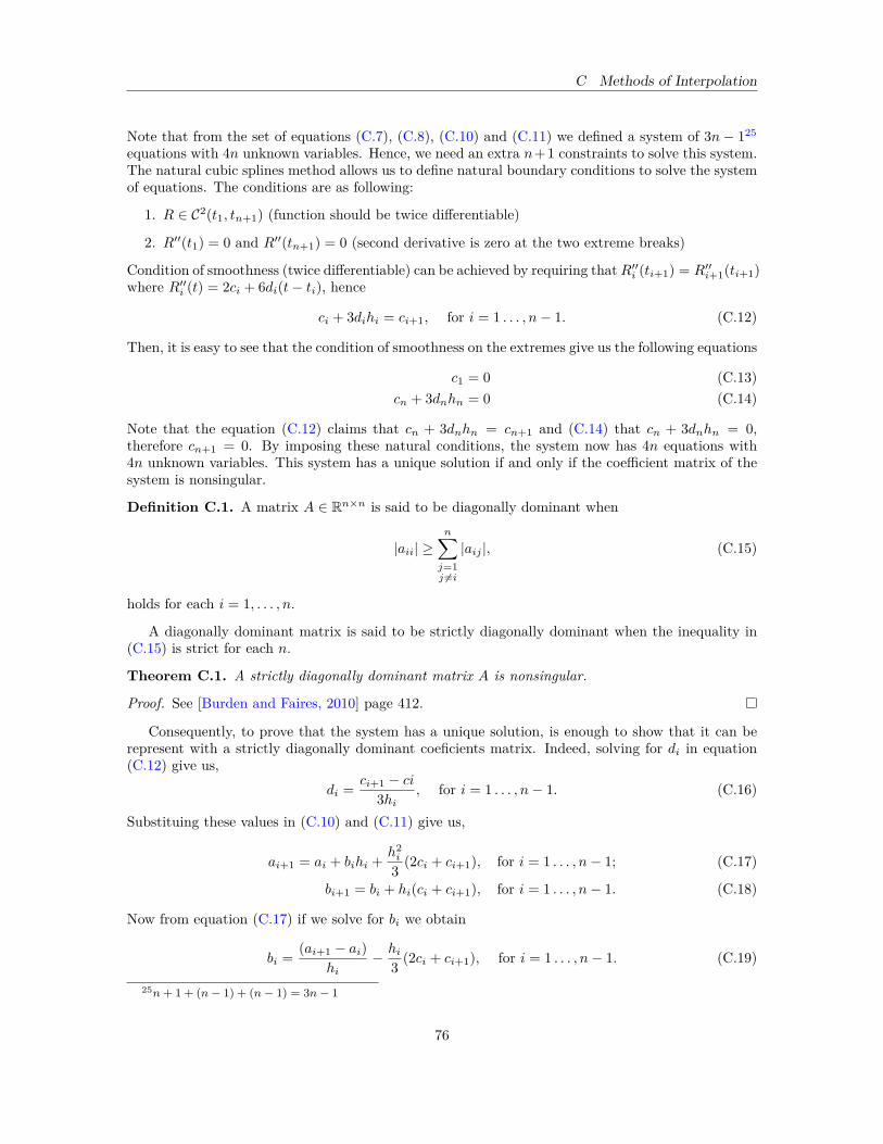
C Methods of Interpolation
Note that from the set of equations (C.7), (C.8), (C.10) and (C.11) we defined a system of 3n− 125
equations with 4n unknown variables. Hence, we need an extra n+1 constraints to solve this system.The natural cubic splines method allows us to define natural boundary conditions to solve the systemof equations. The conditions are as following:
1. R ∈ C2(t1, tn+1) (function should be twice differentiable)
2. R′′(t1) = 0 and R′′(tn+1) = 0 (second derivative is zero at the two extreme breaks)
Condition of smoothness (twice differentiable) can be achieved by requiring thatR′′i (ti+1) = R′′i+1(ti+1)where R′′i (t) = 2ci + 6di(t− ti), hence
ci + 3dihi = ci+1, for i = 1 . . . , n− 1. (C.12)
Then, it is easy to see that the condition of smoothness on the extremes give us the following equations
c1 = 0 (C.13)cn + 3dnhn = 0 (C.14)
Note that the equation (C.12) claims that cn + 3dnhn = cn+1 and (C.14) that cn + 3dnhn = 0,therefore cn+1 = 0. By imposing these natural conditions, the system now has 4n equations with4n unknown variables. This system has a unique solution if and only if the coefficient matrix of thesystem is nonsingular.
Definition C.1. A matrix A ∈ Rn×n is said to be diagonally dominant when
|aii| ≥n∑j=1j 6=i
|aij |, (C.15)
holds for each i = 1, . . . , n.
A diagonally dominant matrix is said to be strictly diagonally dominant when the inequality in(C.15) is strict for each n.
Theorem C.1. A strictly diagonally dominant matrix A is nonsingular.
Proof. See [Burden and Faires, 2010] page 412.
Consequently, to prove that the system has a unique solution, is enough to show that it can berepresent with a strictly diagonally dominant coeficients matrix. Indeed, solving for di in equation(C.12) give us,
di = ci+1 − ci3hi
, for i = 1 . . . , n− 1. (C.16)
Substituing these values in (C.10) and (C.11) give us,
ai+1 = ai + bihi + h2i
3 (2ci + ci+1), for i = 1 . . . , n− 1; (C.17)
bi+1 = bi + hi(ci + ci+1), for i = 1 . . . , n− 1. (C.18)
Now from equation (C.17) if we solve for bi we obtain
bi = (ai+1 − ai)hi
− hi3 (2ci + ci+1), for i = 1 . . . , n− 1. (C.19)
25n + 1 + (n− 1) + (n− 1) = 3n− 1
76
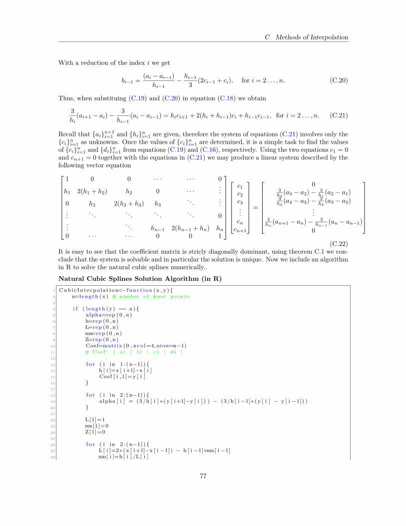
C Methods of Interpolation
With a reduction of the index i we get
bi−1 = (ai − ai−1)hi−1
− hi−1
3 (2ci−1 + ci), for i = 2 . . . , n. (C.20)
Thus, when substituing (C.19) and (C.20) in equation (C.18) we obtain
3hi
(ai+1 − ai)−3
hi−1(ai − ai−1) = hici+1 + 2(hi + hi−1)ci + hi−1ci−1, for i = 2 . . . , n. (C.21)
Recall that ain+1i=1 and hini=1 are given, therefore the system of equations (C.21) involves only the
cini=1 as unknowns. Once the values of cini=1 are determined, it is a simple task to find the valuesof cini=1 and dini=1 from equations (C.19) and (C.16), respectively. Using the two equations c1 = 0and cn+1 = 0 together with the equations in (C.21) we may produce a linear system described by thefollowing vector equation
1 0 0 · · · · · · 0
h1 2(h1 + h2) h2 0 · · ·...
0 h2 2(h2 + h3) h3. . .
......
. . . . . . . . . . . . 0...
. . . hn−1 2(hn−1 + hn) hn0 · · · · · · 0 0 1
c1c2c3...cncn+1
=
03h2
(a3 − a2)− 3h1
(a2 − a1)3h3
(a4 − a3)− 3h2
(a3 − a2)...
3hn
(an+1 − an)− 3hn−1
(an − an−1)0
(C.22)
It is easy to see that the coefficient matrix is stricly diagonally dominant, using theorem C.1 we con-clude that the system is solvable and in particular the solution is unique. Now we include an algorithmin R to solve the natural cubic splines numerically..
Natural Cubic Splines Solution Algorithm (in R)1 Cub i c In t e rpo l a t i on<−f unc t i on (x , y ) 2 n=length (x ) # number o f knot po in t s3
4 i f ( l ength (y ) == n) 5 alpha=rep (0 , n)6 h=rep (0 , n)7 L=rep (0 , n)8 mu=rep (0 , n)9 Z=rep (0 , n)
10 Coef=matrix (0 , nco l=4,nrow=n−1)11 # Coef : [ a i | b i | c i | d i ]12
13 f o r ( i in 1 : ( n−1) ) 14 h [ i ]=x [ i +1]−x [ i ]15 Coef [ i ,1 ]=y [ i ]16 17
18 f o r ( i in 2 : ( n−1) ) 19 alpha [ i ] = (3 /h [ i ] ∗ ( y [ i +1]−y [ i ] ) ) − (3 /h [ i −1]∗ ( y [ i ] − y [ i −1]) )20 21
22 L[1]=123 mu[1]=024 Z[1]=025
26 f o r ( i in 2 : ( n−1) ) 27 L [ i ]=2∗ ( x [ i +1]−x [ i −1]) − h [ i −1]∗mu[ i −1]28 mu[ i ]=h [ i ] /L [ i ]
77
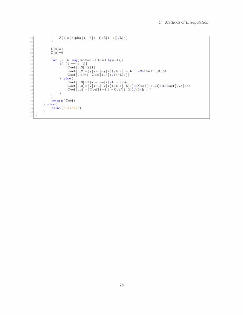
C Methods of Interpolation
29 Z [ i ]=( alpha [ i ]−h [ i −1]∗Z [ i −1]) /L [ i ]30 31
32 L [ n]=133 Z [ n]=034
35 f o r ( i in seq ( from=n−1, to=1,by=−1)) 36 i f ( i == n−1)37 Coef [ i ,3 ]=Z [ i ]38 Coef [ i , 2 ]=( y [ i +1]−y [ i ] ) /h [ i ] − h [ i ] ∗2∗Coef [ i , 3 ] /339 Coef [ i ,4]=(−Coef [ i , 3 ] ) / (3 ∗h [ i ] )40 e l s e 41 Coef [ i ,3 ]=Z [ i ]− mu[ i ] ∗Coef [ i +1 ,3]42 Coef [ i , 2 ]=( y [ i +1]−y [ i ] ) /h [ i ]−h [ i ] ∗ ( Coef [ i +1 ,3]+2∗Coef [ i , 3 ] ) /343 Coef [ i , 4 ]=( Coef [ i +1,3]−Coef [ i , 3 ] ) / (3 ∗h [ i ] )44 45 46 r e turn ( Coef )47 e l s e 48 pr in t ( " Error5 " )49 50
78
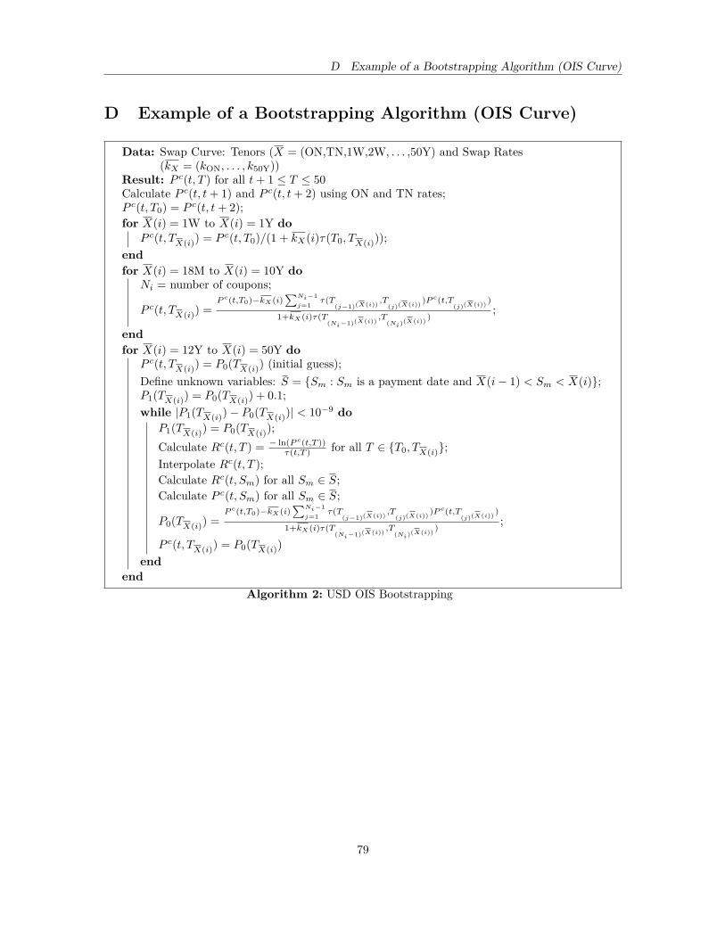
D Example of a Bootstrapping Algorithm (OIS Curve)
D Example of a Bootstrapping Algorithm (OIS Curve)
Data: Swap Curve: Tenors (X = (ON,TN,1W,2W, . . . ,50Y) and Swap Rates(kX = (kON, . . . , k50Y))
Result: P c(t, T ) for all t+ 1 ≤ T ≤ 50Calculate P c(t, t+ 1) and P c(t, t+ 2) using ON and TN rates;P c(t, T0) = P c(t, t+ 2);for X(i) = 1W to X(i) = 1Y do
P c(t, TX(i)) = P c(t, T0)/(1 + kX(i)τ(T0, TX(i)));endfor X(i) = 18M to X(i) = 10Y do
Ni = number of coupons;
P c(t, TX(i)) =P c(t,T0)−kX(i)
∑Ni−1j=1
τ(T(j−1)(X(i)) ,T(j)(X(i)) )P c(t,T
(j)(X(i)) )
1+kX(i)τ(T(Ni−1)(X(i)) ,T(Ni)(X(i)) )
;
endfor X(i) = 12Y to X(i) = 50Y do
P c(t, TX(i)) = P0(TX(i)) (initial guess);Define unknown variables: S = Sm : Sm is a payment date and X(i− 1) < Sm < X(i);P1(TX(i)) = P0(TX(i)) + 0.1;while |P1(TX(i))− P0(TX(i))| < 10−9 do
P1(TX(i)) = P0(TX(i));Calculate Rc(t, T ) = − ln(P c(t,T ))
τ(t,T ) for all T ∈ T0, TX(i);Interpolate Rc(t, T );Calculate Rc(t, Sm) for all Sm ∈ S;Calculate P c(t, Sm) for all Sm ∈ S;
P0(TX(i)) =P c(t,T0)−kX(i)
∑Ni−1j=1
τ(T(j−1)(X(i)) ,T(j)(X(i)) )P c(t,T
(j)(X(i)) )
1+kX(i)τ(T(Ni−1)(X(i)) ,T(Ni)(X(i)) )
;
P c(t, TX(i)) = P0(TX(i))end
endAlgorithm 2: USD OIS Bootstrapping
79
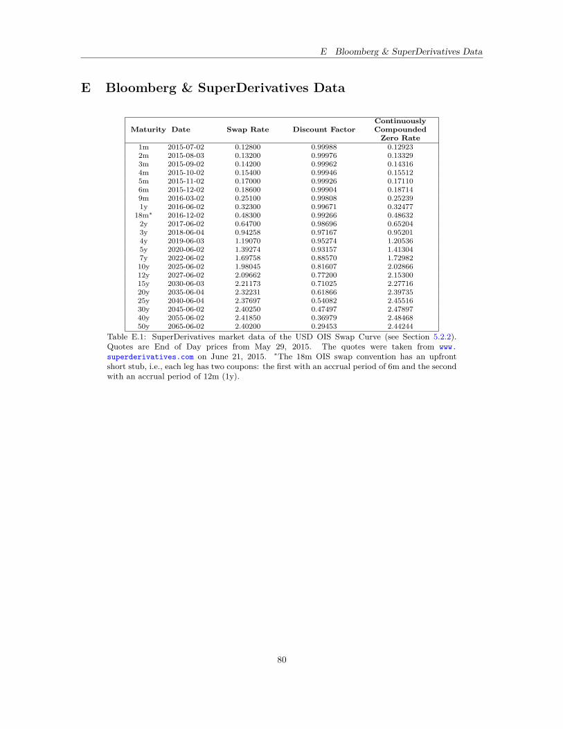
E Bloomberg & SuperDerivatives Data
E Bloomberg & SuperDerivatives Data
Maturity Date Swap Rate Discount FactorContinuouslyCompounded
Zero Rate1m 2015-07-02 0.12800 0.99988 0.129232m 2015-08-03 0.13200 0.99976 0.133293m 2015-09-02 0.14200 0.99962 0.143164m 2015-10-02 0.15400 0.99946 0.155125m 2015-11-02 0.17000 0.99926 0.171106m 2015-12-02 0.18600 0.99904 0.187149m 2016-03-02 0.25100 0.99808 0.252391y 2016-06-02 0.32300 0.99671 0.32477
18m∗ 2016-12-02 0.48300 0.99266 0.486322y 2017-06-02 0.64700 0.98696 0.652043y 2018-06-04 0.94258 0.97167 0.952014y 2019-06-03 1.19070 0.95274 1.205365y 2020-06-02 1.39274 0.93157 1.413047y 2022-06-02 1.69758 0.88570 1.7298210y 2025-06-02 1.98045 0.81607 2.0286612y 2027-06-02 2.09662 0.77200 2.1530015y 2030-06-03 2.21173 0.71025 2.2771620y 2035-06-04 2.32231 0.61866 2.3973525y 2040-06-04 2.37697 0.54082 2.4551630y 2045-06-02 2.40250 0.47497 2.4789740y 2055-06-02 2.41850 0.36979 2.4846850y 2065-06-02 2.40200 0.29453 2.44244
Table E.1: SuperDerivatives market data of the USD OIS Swap Curve (see Section 5.2.2).Quotes are End of Day prices from May 29, 2015. The quotes were taken from www.superderivatives.com on June 21, 2015. ∗The 18m OIS swap convention has an upfrontshort stub, i.e., each leg has two coupons: the first with an accrual period of 6m and the secondwith an accrual period of 12m (1y).
80
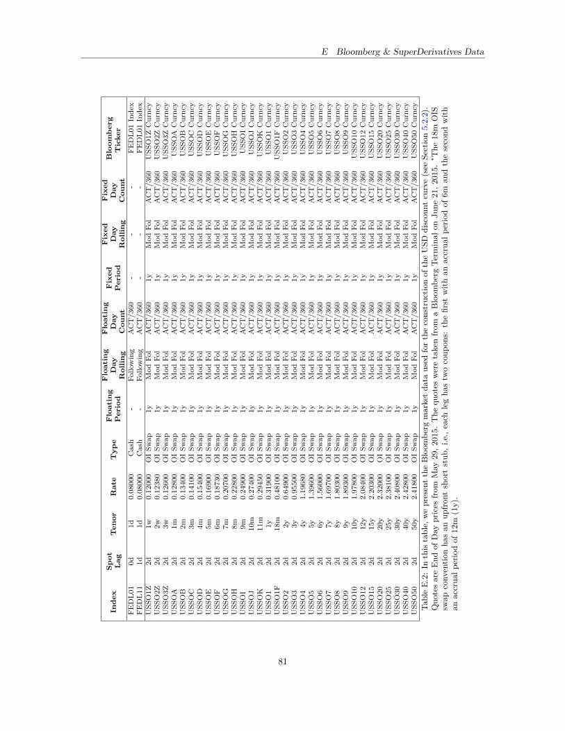
E Bloomberg & SuperDerivatives Data
Inde
xSp
otL
agT
enor
Rat
eT
ype
Flo
atin
gP
erio
dF
loat
ing
Day
Rol
ling
Flo
atin
gD
ayC
ount
Fix
edP
erio
dF
ixed
Day
Rol
ling
Fix
edD
ayC
ount
Blo
omb
erg
Tic
ker
FEDL0
10d
1d0.08
000
Cash
-Fo
llowing
ACT/360
--
-FEDL0
1Inde
xFEDL1
11d
1d0.08
000
Cash
-Fo
llowing
ACT/360
--
-FEDL0
1Inde
xUSS
O1Z
2d1w
0.1200
0OISw
ap1y
Mod
Fol
ACT/360
1yMod
Fol
ACT/360
USS
O1Z
Curncy
USS
O2Z
2d2w
0.1238
0OISw
ap1y
Mod
Fol
ACT/360
1yMod
Fol
ACT/360
USS
O2Z
Curncy
USS
O3Z
2d3w
0.1260
0OISw
ap1y
Mod
Fol
ACT/360
1yMod
Fol
ACT/360
USS
O3Z
Curncy
USS
OA
2d1m
0.12
800
OISw
ap1y
Mod
Fol
ACT/360
1yMod
Fol
ACT/360
USS
OA
Curncy
USS
OB
2d2m
0.13
400
OISw
ap1y
Mod
Fol
ACT/360
1yMod
Fol
ACT/360
USS
OB
Curncy
USS
OC
2d3m
0.14
100
OISw
ap1y
Mod
Fol
ACT/360
1yMod
Fol
ACT/360
USS
OC
Curncy
USS
OD
2d4m
0.15
400
OISw
ap1y
Mod
Fol
ACT/360
1yMod
Fol
ACT/360
USS
OD
Curncy
USS
OE
2d5m
0.1690
0OISw
ap1y
Mod
Fol
ACT/360
1yMod
Fol
ACT/360
USS
OE
Curncy
USS
OF
2d6m
0.18
730
OISw
ap1y
Mod
Fol
ACT/360
1yMod
Fol
ACT/360
USS
OFCurncy
USS
OG
2d7m
0.20
700
OISw
ap1y
Mod
Fol
ACT/360
1yMod
Fol
ACT/360
USS
OG
Curncy
USS
OH
2d8m
0.22
800
OISw
ap1y
Mod
Fol
ACT/360
1yMod
Fol
ACT/360
USS
OH
Curncy
USS
OI
2d9m
0.2490
0OISw
ap1y
Mod
Fol
ACT/360
1yMod
Fol
ACT/360
USS
OICurncy
USS
OJ
2d10
m0.27
400
OISw
ap1y
Mod
Fol
ACT/360
1yMod
Fol
ACT/360
USS
OJCurncy
USS
OK
2d11
m0.29
450
OISw
ap1y
Mod
Fol
ACT/360
1yMod
Fol
ACT/360
USS
OK
Curncy
USS
O1
2d1y
0.3190
0OISw
ap1y
Mod
Fol
ACT/360
1yMod
Fol
ACT/360
USS
O1Curncy
USS
O1F
2d18
m0.48
100
OISw
ap1y
Mod
Fol
ACT/360
1yMod
Fol
ACT/360
USS
O1F
Curncy
USS
O2
2d2y
0.6490
0OISw
ap1y
Mod
Fol
ACT/360
1yMod
Fol
ACT/360
USS
O2Curncy
USS
O3
2d3y
0.9550
0OISw
ap1y
Mod
Fol
ACT/360
1yMod
Fol
ACT/360
USS
O3Curncy
USS
O4
2d4y
1.1968
0OISw
ap1y
Mod
Fol
ACT/360
1yMod
Fol
ACT/360
USS
O4Curncy
USS
O5
2d5y
1.3960
0OISw
ap1y
Mod
Fol
ACT/360
1yMod
Fol
ACT/360
USS
O5Curncy
USS
O6
2d6y
1.5600
0OISw
ap1y
Mod
Fol
ACT/360
1yMod
Fol
ACT/360
USS
O6Curncy
USS
O7
2d7y
1.6970
0OISw
ap1y
Mod
Fol
ACT/360
1yMod
Fol
ACT/360
USS
O7Curncy
USS
O8
2d8y
1.8030
0OISw
ap1y
Mod
Fol
ACT/360
1yMod
Fol
ACT/360
USS
O8Curncy
USS
O9
2d9y
1.8930
0OISw
ap1y
Mod
Fol
ACT/360
1yMod
Fol
ACT/360
USS
O9Curncy
USS
O10
2d10
y1.97
800
OISw
ap1y
Mod
Fol
ACT/360
1yMod
Fol
ACT/360
USS
O10
Curncy
USS
O12
2d12
y2.08
400
OISw
ap1y
Mod
Fol
ACT/360
1yMod
Fol
ACT/360
USS
O12
Curncy
USS
O15
2d15
y2.20
300
OISw
ap1y
Mod
Fol
ACT/360
1yMod
Fol
ACT/360
USS
O15
Curncy
USS
O20
2d20
y2.32
000
OISw
ap1y
Mod
Fol
ACT/360
1yMod
Fol
ACT/360
USS
O20
Curncy
USS
O25
2d25
y2.38
100
OISw
ap1y
Mod
Fol
ACT/360
1yMod
Fol
ACT/360
USS
O25
Curncy
USS
O30
2d30
y2.40
800
OISw
ap1y
Mod
Fol
ACT/360
1yMod
Fol
ACT/360
USS
O30
Curncy
USS
O40
2d40
y2.42
800
OISw
ap1y
Mod
Fol
ACT/360
1yMod
Fol
ACT/360
USS
O40
Curncy
USS
O50
2d50
y2.41
800
OISw
ap1y
Mod
Fol
ACT/360
1yMod
Fol
ACT/360
USS
O50
Curncy
TableE.2:In
thistable,
wepresenttheBloom
berg
marketda
taused
fortheconstructio
nof
theUSD
discou
ntcurve(see
Section5.2.2).
Quo
tesareEnd
ofDay
prices
from
May
29,2
015.
The
quotes
weretakenfrom
aBloom
berg
Term
inal
onJu
ne21,2
015.∗The
18m
OIS
swap
conv
entio
nha
san
upfron
tshortstub
,i.e.,each
legha
stw
ocoup
ons:
thefirst
with
anaccrua
lperiodof
6man
dthesecond
with
anaccrua
lperiodof
12m
(1y).
81
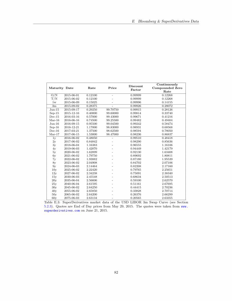
E Bloomberg & SuperDerivatives Data
Maturity Date Rate Price DiscountFactor
ContinuouslyCompounded Zero
RateO/N 2015-06-01 0.12100 - 0.99999 0.12268T/N 2015-06-02 0.12100 - 0.99999 0.122681w 2015-06-09 0.15025 - 0.99996 0.141553m 2015-09-02 0.28375 - 0.99926 0.28072
Jun-15 2015-09-17 0.29250 99.70750 0.99915 0.28126Sep-15 2015-12-16 0.40000 99.60000 0.99814 0.33740Dec-15 2016-03-16 0.57000 99.43000 0.99671 0.41216Mar-16 2016-06-16 0.74500 99.25500 0.99482 0.49404Jun-16 2016-09-15 0.95500 99.04500 0.99242 0.58474Sep-16 2016-12-21 1.17000 98.83000 0.98931 0.68568Dec-16 2017-03-21 1.37500 98.62500 0.98594 0.78050Mar-17 2017-06-15 1.53000 98.47000 0.98236 0.86837
1y 2016-06-02 0.48050 - 0.99510 0.484182y 2017-06-02 0.84842 - 0.98290 0.856363y 2018-06-04 1.16383 - 0.96555 1.161064y 2019-06-03 1.42070 - 0.94449 1.421795y 2020-06-02 1.62899 - 0.92130 1.634086y 2021-06-02 1.79750 - 0.89692 1.808117y 2022-06-02 1.93882 - 0.87180 1.955398y 2023-06-02 2.04908 - 0.84702 2.071069y 2024-06-03 2.14464 - 0.82208 2.1716010y 2025-06-02 2.22420 - 0.79765 2.2565112y 2027-06-02 2.34238 - 0.75091 2.3834015y 2030-06-03 2.45548 - 0.68634 2.5051320y 2035-06-04 2.56606 - 0.59100 2.6257025y 2040-06-04 2.61595 - 0.51161 2.6769530y 2045-06-02 2.64250 - 0.44415 2.7023640y 2055-06-02 2.65850 - 0.33828 2.7071450y 2065-06-02 2.64200 - 0.26376 2.6629960y 2075-06-03 2.63134 - 0.20565 2.63355
Table E.3: SuperDerivatives market data of the USD LIBOR 3m Swap Curve (see Section5.2.3). Quotes are End of Day prices from May 29, 2015. The quotes were taken from www.superderivatives.com on June 21, 2015.
82
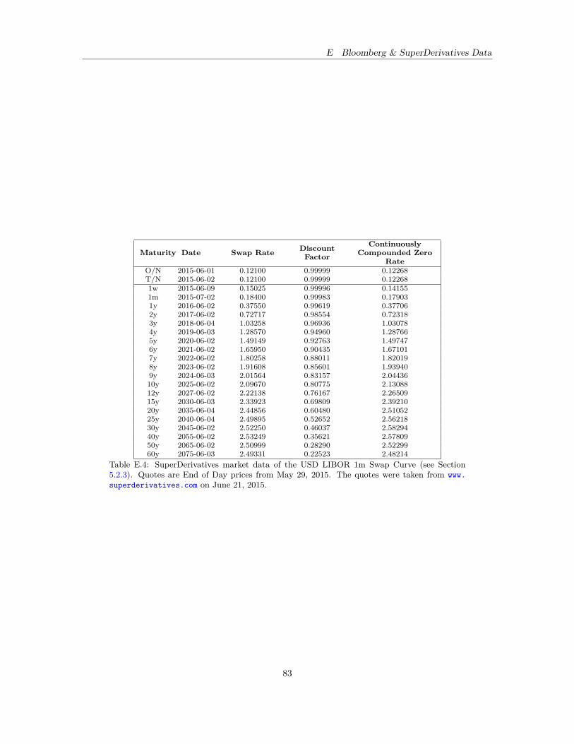
E Bloomberg & SuperDerivatives Data
Maturity Date Swap Rate DiscountFactor
ContinuouslyCompounded Zero
RateO/N 2015-06-01 0.12100 0.99999 0.12268T/N 2015-06-02 0.12100 0.99999 0.122681w 2015-06-09 0.15025 0.99996 0.141551m 2015-07-02 0.18400 0.99983 0.179031y 2016-06-02 0.37550 0.99619 0.377062y 2017-06-02 0.72717 0.98554 0.723183y 2018-06-04 1.03258 0.96936 1.030784y 2019-06-03 1.28570 0.94960 1.287665y 2020-06-02 1.49149 0.92763 1.497476y 2021-06-02 1.65950 0.90435 1.671017y 2022-06-02 1.80258 0.88011 1.820198y 2023-06-02 1.91608 0.85601 1.939409y 2024-06-03 2.01564 0.83157 2.0443610y 2025-06-02 2.09670 0.80775 2.1308812y 2027-06-02 2.22138 0.76167 2.2650915y 2030-06-03 2.33923 0.69809 2.3921020y 2035-06-04 2.44856 0.60480 2.5105225y 2040-06-04 2.49895 0.52652 2.5621830y 2045-06-02 2.52250 0.46037 2.5829440y 2055-06-02 2.53249 0.35621 2.5780950y 2065-06-02 2.50999 0.28290 2.5229960y 2075-06-03 2.49331 0.22523 2.48214
Table E.4: SuperDerivatives market data of the USD LIBOR 1m Swap Curve (see Section5.2.3). Quotes are End of Day prices from May 29, 2015. The quotes were taken from www.superderivatives.com on June 21, 2015.
83
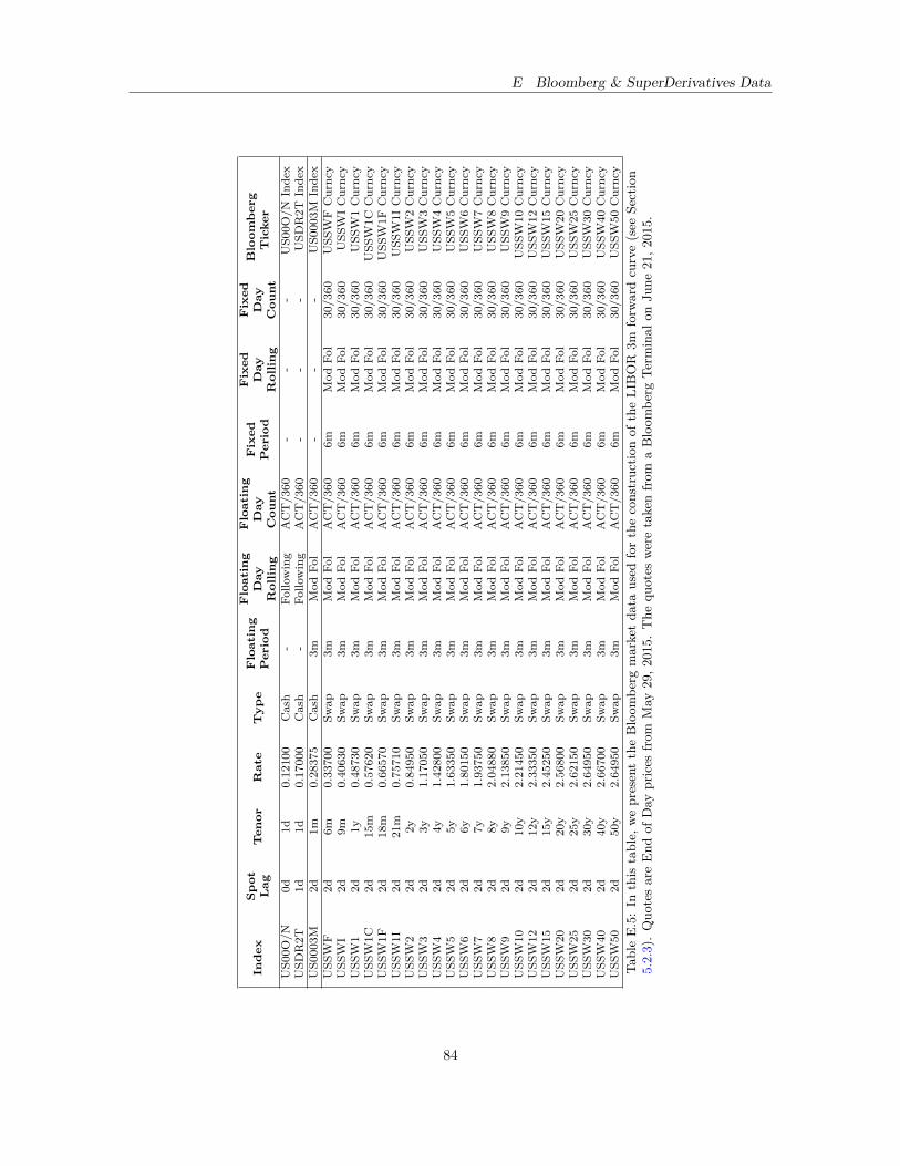
E Bloomberg & SuperDerivatives Data
Inde
xSp
otL
agT
enor
Rat
eT
ype
Flo
atin
gP
erio
dF
loat
ing
Day
Rol
ling
Flo
atin
gD
ayC
ount
Fix
edP
erio
dF
ixed
Day
Rol
ling
Fix
edD
ayC
ount
Blo
omb
erg
Tic
ker
US0
0O/N
0d1d
0.12
100
Cash
-Fo
llowing
ACT/360
--
-US0
0O/N
Index
USD
R2T
1d1d
0.17
000
Cash
-Fo
llowing
ACT/360
--
-USD
R2T
Index
US0
003M
2d1m
0.28
375
Cash
3mMod
Fol
ACT/360
--
-US0
003M
Index
USS
WF
2d6m
0.33
700
Swap
3mMod
Fol
ACT/360
6mMod
Fol
30/360
USS
WFCurncy
USS
WI
2d9m
0.40
630
Swap
3mMod
Fol
ACT/360
6mMod
Fol
30/360
USS
WICurncy
USS
W1
2d1y
0.48
730
Swap
3mMod
Fol
ACT/360
6mMod
Fol
30/360
USS
W1Curncy
USS
W1C
2d15
m0.57
620
Swap
3mMod
Fol
ACT/360
6mMod
Fol
30/360
USS
W1C
Curncy
USS
W1F
2d18m
0.66
570
Swap
3mMod
Fol
ACT/360
6mMod
Fol
30/360
USS
W1F
Curncy
USS
W1I
2d21
m0.75
710
Swap
3mMod
Fol
ACT/360
6mMod
Fol
30/360
USS
W1I
Curncy
USS
W2
2d2y
0.84
950
Swap
3mMod
Fol
ACT/360
6mMod
Fol
30/360
USS
W2Curncy
USS
W3
2d3y
1.17
050
Swap
3mMod
Fol
ACT/360
6mMod
Fol
30/360
USS
W3Curncy
USS
W4
2d4y
1.42
800
Swap
3mMod
Fol
ACT/360
6mMod
Fol
30/360
USS
W4Curncy
USS
W5
2d5y
1.63
350
Swap
3mMod
Fol
ACT/360
6mMod
Fol
30/360
USS
W5Curncy
USS
W6
2d6y
1.80
150
Swap
3mMod
Fol
ACT/360
6mMod
Fol
30/360
USS
W6Curncy
USS
W7
2d7y
1.93
750
Swap
3mMod
Fol
ACT/360
6mMod
Fol
30/360
USS
W7Curncy
USS
W8
2d8y
2.04
880
Swap
3mMod
Fol
ACT/360
6mMod
Fol
30/360
USS
W8Curncy
USS
W9
2d9y
2.13
850
Swap
3mMod
Fol
ACT/360
6mMod
Fol
30/360
USS
W9Curncy
USS
W10
2d10
y2.21
450
Swap
3mMod
Fol
ACT/360
6mMod
Fol
30/360
USS
W10
Curncy
USS
W12
2d12
y2.33
350
Swap
3mMod
Fol
ACT/360
6mMod
Fol
30/360
USS
W12
Curncy
USS
W15
2d15
y2.45
250
Swap
3mMod
Fol
ACT/360
6mMod
Fol
30/360
USS
W15
Curncy
USS
W20
2d20
y2.56
800
Swap
3mMod
Fol
ACT/360
6mMod
Fol
30/360
USS
W20
Curncy
USS
W25
2d25
y2.62
150
Swap
3mMod
Fol
ACT/360
6mMod
Fol
30/360
USS
W25
Curncy
USS
W30
2d30
y2.64
950
Swap
3mMod
Fol
ACT/360
6mMod
Fol
30/360
USS
W30
Curncy
USS
W40
2d40
y2.66
700
Swap
3mMod
Fol
ACT/360
6mMod
Fol
30/360
USS
W40
Curncy
USS
W50
2d50
y2.64
950
Swap
3mMod
Fol
ACT/360
6mMod
Fol
30/360
USS
W50
Curncy
TableE.5:In
this
table,
wepresenttheBloom
berg
marketda
taused
fortheconstructio
nof
theLIBOR
3mforw
ardcurve(see
Section
5.2.3).Quo
tesareEnd
ofDay
prices
from
May
29,2
015.
The
quotes
weretakenfrom
aBloom
berg
Term
inal
onJu
ne21,2
015.
84
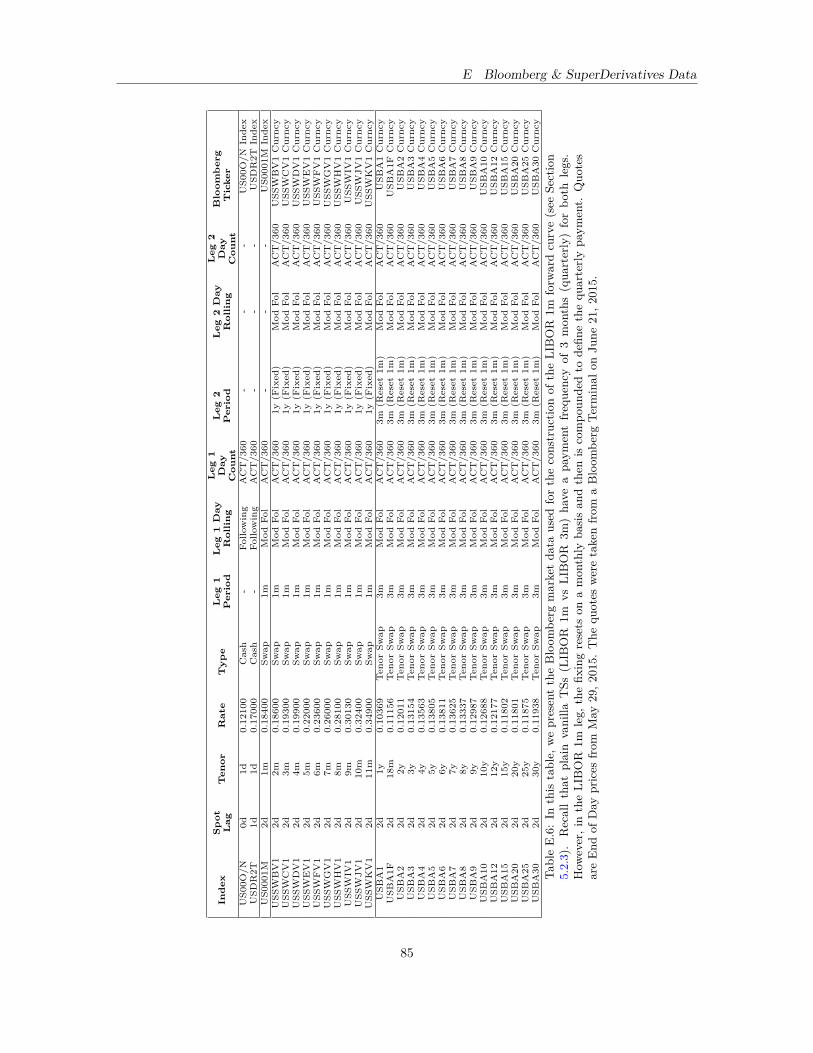
E Bloomberg & SuperDerivatives Data
Ind
exS
pot
Lag
Ten
orR
ate
Typ
eL
eg1
Per
iod
Leg
1D
ayR
olli
ng
Leg
1D
ayC
ount
Leg
2P
erio
dL
eg2
Day
Rol
lin
gL
eg2
Day
Cou
ntB
loom
ber
gT
icke
rU
S00O
/N0d
1d0.
1210
0C
ash
-Fo
llow
ing
AC
T/3
60-
--
US0
0O/N
Inde
xU
SDR
2T1d
1d0.
1700
0C
ash
-Fo
llow
ing
AC
T/3
60-
--
USD
R2T
Inde
xU
S000
1M2d
1m0.
1840
0Sw
ap1m
Mod
Fol
AC
T/3
60-
--
US0
001M
Inde
xU
SSW
BV
12d
2m0.
1860
0Sw
ap1m
Mod
Fol
AC
T/3
601y
(Fix
ed)
Mod
Fol
AC
T/3
60U
SSW
BV
1C
urnc
yU
SSW
CV
12d
3m0.
1930
0Sw
ap1m
Mod
Fol
AC
T/3
601y
(Fix
ed)
Mod
Fol
AC
T/3
60U
SSW
CV
1C
urnc
yU
SSW
DV
12d
4m0.
1990
0Sw
ap1m
Mod
Fol
AC
T/3
601y
(Fix
ed)
Mod
Fol
AC
T/3
60U
SSW
DV
1C
urnc
yU
SSW
EV
12d
5m0.
2200
0Sw
ap1m
Mod
Fol
AC
T/3
601y
(Fix
ed)
Mod
Fol
AC
T/3
60U
SSW
EV
1C
urnc
yU
SSW
FV
12d
6m0.
2360
0Sw
ap1m
Mod
Fol
AC
T/3
601y
(Fix
ed)
Mod
Fol
AC
T/3
60U
SSW
FV
1C
urnc
yU
SSW
GV
12d
7m0.
2600
0Sw
ap1m
Mod
Fol
AC
T/3
601y
(Fix
ed)
Mod
Fol
AC
T/3
60U
SSW
GV
1C
urnc
yU
SSW
HV
12d
8m0.
2810
0Sw
ap1m
Mod
Fol
AC
T/3
601y
(Fix
ed)
Mod
Fol
AC
T/3
60U
SSW
HV
1C
urnc
yU
SSW
IV1
2d9m
0.30
130
Swap
1mM
odFo
lA
CT
/360
1y(F
ixed
)M
odFo
lA
CT
/360
USS
WIV
1C
urnc
yU
SSW
JV1
2d10
m0.
3240
0Sw
ap1m
Mod
Fol
AC
T/3
601y
(Fix
ed)
Mod
Fol
AC
T/3
60U
SSW
JV1
Cur
ncy
USS
WK
V1
2d11
m0.
3490
0Sw
ap1m
Mod
Fol
AC
T/3
601y
(Fix
ed)
Mod
Fol
AC
T/3
60U
SSW
KV
1C
urnc
yU
SBA
12d
1y0.
1036
9T
enor
Swap
3mM
odFo
lA
CT
/360
3m(R
eset
1m)
Mod
Fol
AC
T/3
60U
SBA
1C
urnc
yU
SBA
1F2d
18m
0.11
156
Ten
orSw
ap3m
Mod
Fol
AC
T/3
603m
(Res
et1m
)M
odFo
lA
CT
/360
USB
A1F
Cur
ncy
USB
A2
2d2y
0.12
011
Ten
orSw
ap3m
Mod
Fol
AC
T/3
603m
(Res
et1m
)M
odFo
lA
CT
/360
USB
A2
Cur
ncy
USB
A3
2d3y
0.13
154
Ten
orSw
ap3m
Mod
Fol
AC
T/3
603m
(Res
et1m
)M
odFo
lA
CT
/360
USB
A3
Cur
ncy
USB
A4
2d4y
0.13
563
Ten
orSw
ap3m
Mod
Fol
AC
T/3
603m
(Res
et1m
)M
odFo
lA
CT
/360
USB
A4
Cur
ncy
USB
A5
2d5y
0.13
805
Ten
orSw
ap3m
Mod
Fol
AC
T/3
603m
(Res
et1m
)M
odFo
lA
CT
/360
USB
A5
Cur
ncy
USB
A6
2d6y
0.13
811
Ten
orSw
ap3m
Mod
Fol
AC
T/3
603m
(Res
et1m
)M
odFo
lA
CT
/360
USB
A6
Cur
ncy
USB
A7
2d7y
0.13
625
Ten
orSw
ap3m
Mod
Fol
AC
T/3
603m
(Res
et1m
)M
odFo
lA
CT
/360
USB
A7
Cur
ncy
USB
A8
2d8y
0.13
337
Ten
orSw
ap3m
Mod
Fol
AC
T/3
603m
(Res
et1m
)M
odFo
lA
CT
/360
USB
A8
Cur
ncy
USB
A9
2d9y
0.12
987
Ten
orSw
ap3m
Mod
Fol
AC
T/3
603m
(Res
et1m
)M
odFo
lA
CT
/360
USB
A9
Cur
ncy
USB
A10
2d10
y0.
1268
8T
enor
Swap
3mM
odFo
lA
CT
/360
3m(R
eset
1m)
Mod
Fol
AC
T/3
60U
SBA
10C
urnc
yU
SBA
122d
12y
0.12
177
Ten
orSw
ap3m
Mod
Fol
AC
T/3
603m
(Res
et1m
)M
odFo
lA
CT
/360
USB
A12
Cur
ncy
USB
A15
2d15
y0.
1180
2T
enor
Swap
3mM
odFo
lA
CT
/360
3m(R
eset
1m)
Mod
Fol
AC
T/3
60U
SBA
15C
urnc
yU
SBA
202d
20y
0.11
801
Ten
orSw
ap3m
Mod
Fol
AC
T/3
603m
(Res
et1m
)M
odFo
lA
CT
/360
USB
A20
Cur
ncy
USB
A25
2d25
y0.
1187
5T
enor
Swap
3mM
odFo
lA
CT
/360
3m(R
eset
1m)
Mod
Fol
AC
T/3
60U
SBA
25C
urnc
yU
SBA
302d
30y
0.11
938
Ten
orSw
ap3m
Mod
Fol
AC
T/3
603m
(Res
et1m
)M
odFo
lA
CT
/360
USB
A30
Cur
ncy
TableE.6:In
this
table,
wepresenttheBloom
berg
marketda
taused
fortheconstructio
nof
theLIBOR
1mforw
ardcurve(see
Section
5.2.3).
Recallthat
plainvanilla
TSs
(LIB
OR
1mvs
LIBOR
3m)ha
veapa
ymentfreque
ncyof
3mon
ths(qua
rterly)forbo
thlegs.
How
ever,intheLIBOR
1mleg,
thefix
ingresets
onamon
thly
basisan
dthen
iscompo
unde
dto
defin
ethequ
arterly
paym
ent.
Quo
tes
areEnd
ofDay
prices
from
May
29,2
015.
The
quotes
weretakenfrom
aBloom
berg
Term
inal
onJu
ne21,2
015.
85
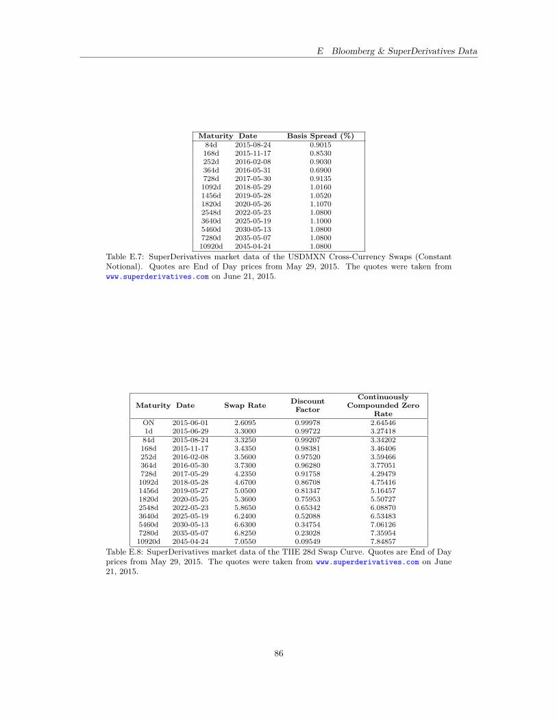
E Bloomberg & SuperDerivatives Data
Maturity Date Basis Spread (%)84d 2015-08-24 0.9015168d 2015-11-17 0.8530252d 2016-02-08 0.9030364d 2016-05-31 0.6900728d 2017-05-30 0.91351092d 2018-05-29 1.01601456d 2019-05-28 1.05201820d 2020-05-26 1.10702548d 2022-05-23 1.08003640d 2025-05-19 1.10005460d 2030-05-13 1.08007280d 2035-05-07 1.080010920d 2045-04-24 1.0800
Table E.7: SuperDerivatives market data of the USDMXN Cross-Currency Swaps (ConstantNotional). Quotes are End of Day prices from May 29, 2015. The quotes were taken fromwww.superderivatives.com on June 21, 2015.
Maturity Date Swap Rate DiscountFactor
ContinuouslyCompounded Zero
RateON 2015-06-01 2.6095 0.99978 2.645461d 2015-06-29 3.3000 0.99722 3.2741884d 2015-08-24 3.3250 0.99207 3.34202168d 2015-11-17 3.4350 0.98381 3.46406252d 2016-02-08 3.5600 0.97520 3.59466364d 2016-05-30 3.7300 0.96280 3.77051728d 2017-05-29 4.2350 0.91758 4.294791092d 2018-05-28 4.6700 0.86708 4.754161456d 2019-05-27 5.0500 0.81347 5.164571820d 2020-05-25 5.3600 0.75953 5.507272548d 2022-05-23 5.8650 0.65342 6.088703640d 2025-05-19 6.2400 0.52088 6.534835460d 2030-05-13 6.6300 0.34754 7.061267280d 2035-05-07 6.8250 0.23028 7.3595410920d 2045-04-24 7.0550 0.09549 7.84857
Table E.8: SuperDerivatives market data of the TIIE 28d Swap Curve. Quotes are End of Dayprices from May 29, 2015. The quotes were taken from www.superderivatives.com on June21, 2015.
86
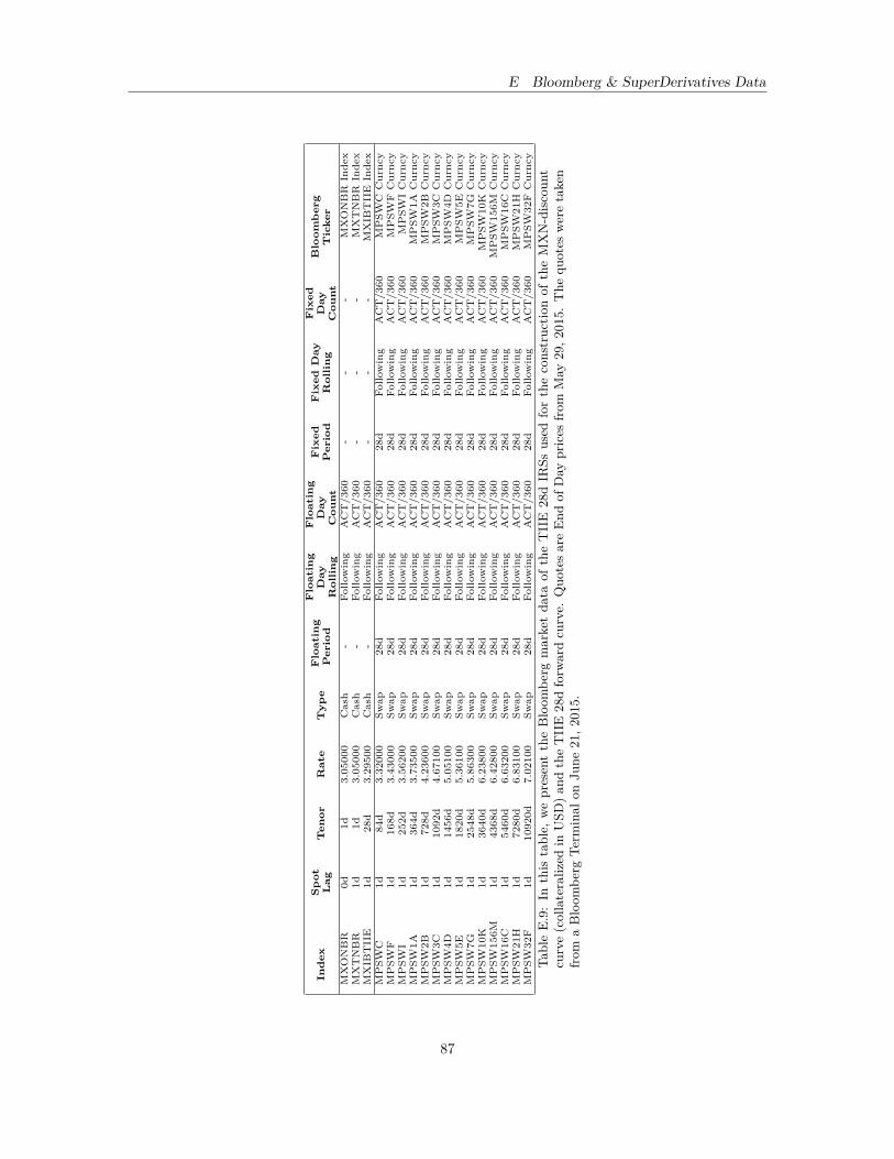
E Bloomberg & SuperDerivatives Data
Ind
exS
pot
Lag
Ten
orR
ate
Typ
eF
loat
ing
Per
iod
Flo
atin
gD
ayR
olli
ng
Flo
atin
gD
ayC
ount
Fix
edP
erio
dF
ixed
Day
Rol
lin
gF
ixed
Day
Cou
ntB
loom
ber
gT
icke
rM
XO
NB
R0d
1d3.
0500
0C
ash
-Fo
llow
ing
AC
T/3
60-
--
MX
ON
BR
Inde
xM
XT
NB
R1d
1d3.
0500
0C
ash
-Fo
llow
ing
AC
T/3
60-
--
MX
TN
BR
Inde
xM
XIB
TII
E1d
28d
3.29
500
Cas
h-
Follo
win
gA
CT
/360
--
-M
XIB
TII
EIn
dex
MP
SWC
1d84
d3.
3200
0Sw
ap28
dFo
llow
ing
AC
T/3
6028
dFo
llow
ing
AC
T/3
60M
PSW
CC
urnc
yM
PSW
F1d
168d
3.43
000
Swap
28d
Follo
win
gA
CT
/360
28d
Follo
win
gA
CT
/360
MP
SWF
Cur
ncy
MP
SWI
1d25
2d3.
5620
0Sw
ap28
dFo
llow
ing
AC
T/3
6028
dFo
llow
ing
AC
T/3
60M
PSW
IC
urnc
yM
PSW
1A1d
364d
3.73
500
Swap
28d
Follo
win
gA
CT
/360
28d
Follo
win
gA
CT
/360
MP
SW1A
Cur
ncy
MP
SW2B
1d72
8d4.
2360
0Sw
ap28
dFo
llow
ing
AC
T/3
6028
dFo
llow
ing
AC
T/3
60M
PSW
2BC
urnc
yM
PSW
3C1d
1092
d4.
6710
0Sw
ap28
dFo
llow
ing
AC
T/3
6028
dFo
llow
ing
AC
T/3
60M
PSW
3CC
urnc
yM
PSW
4D1d
1456
d5.
0510
0Sw
ap28
dFo
llow
ing
AC
T/3
6028
dFo
llow
ing
AC
T/3
60M
PSW
4DC
urnc
yM
PSW
5E1d
1820
d5.
3610
0Sw
ap28
dFo
llow
ing
AC
T/3
6028
dFo
llow
ing
AC
T/3
60M
PSW
5EC
urnc
yM
PSW
7G1d
2548
d5.
8630
0Sw
ap28
dFo
llow
ing
AC
T/3
6028
dFo
llow
ing
AC
T/3
60M
PSW
7GC
urnc
yM
PSW
10K
1d36
40d
6.23
800
Swap
28d
Follo
win
gA
CT
/360
28d
Follo
win
gA
CT
/360
MP
SW10
KC
urnc
yM
PSW
156M
1d43
68d
6.42
800
Swap
28d
Follo
win
gA
CT
/360
28d
Follo
win
gA
CT
/360
MP
SW15
6MC
urnc
yM
PSW
16C
1d54
60d
6.63
200
Swap
28d
Follo
win
gA
CT
/360
28d
Follo
win
gA
CT
/360
MP
SW16
CC
urnc
yM
PSW
21H
1d72
80d
6.83
100
Swap
28d
Follo
win
gA
CT
/360
28d
Follo
win
gA
CT
/360
MP
SW21
HC
urnc
yM
PSW
32F
1d10
920d
7.02
100
Swap
28d
Follo
win
gA
CT
/360
28d
Follo
win
gA
CT
/360
MP
SW32
FC
urnc
yTa
bleE.9:In
this
table,
wepresenttheBloom
berg
marketda
taof
theTIIE
28dIR
Ssused
fortheconstructio
nof
theMXN-discoun
tcurve(collateralized
inUSD
)an
dtheTIIE28dforw
ardcurve.
Quo
tesareEnd
ofDay
prices
from
May
29,2
015.
The
quotes
weretaken
from
aBloom
berg
Term
inal
onJu
ne21,2
015.
87
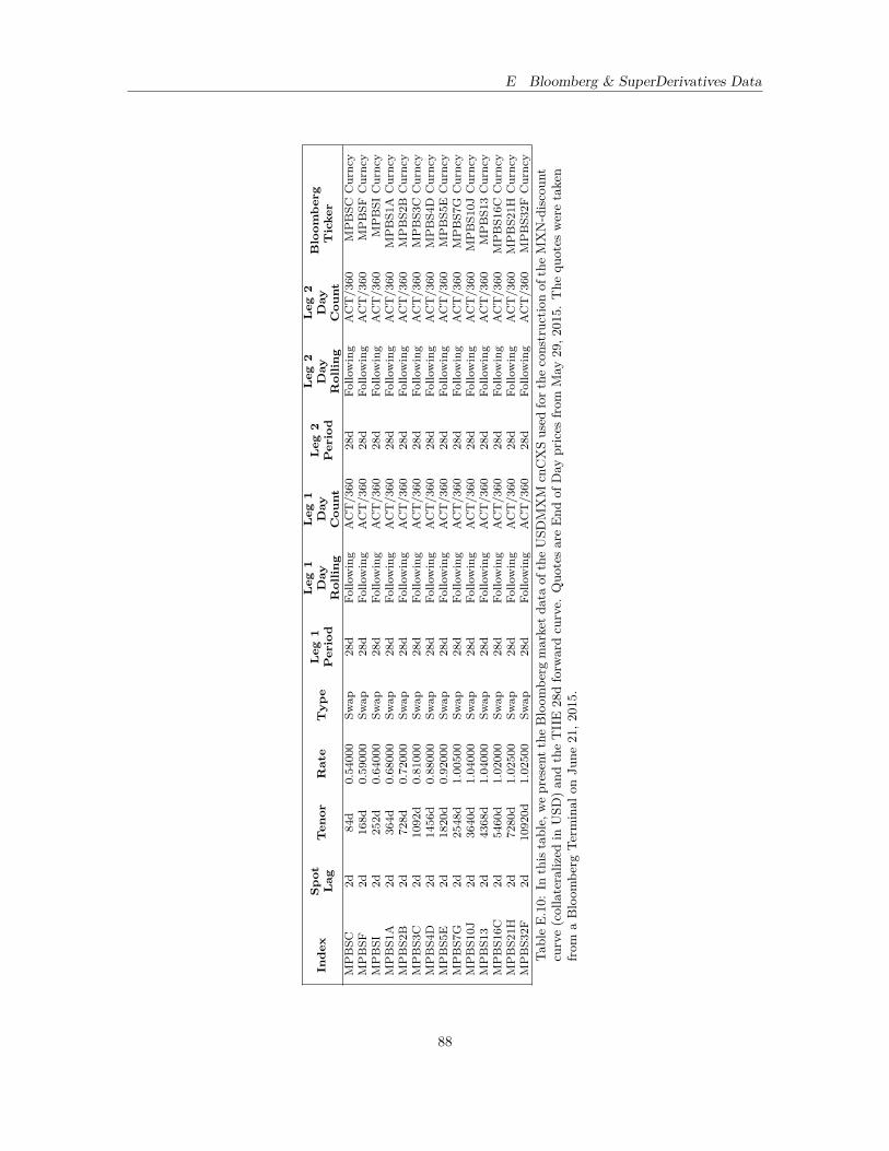
E Bloomberg & SuperDerivatives Data
Inde
xSp
otL
agT
enor
Rat
eT
ype
Leg
1P
erio
dL
eg1
Day
Rol
ling
Leg
1D
ayC
ount
Leg
2P
erio
dL
eg2
Day
Rol
ling
Leg
2D
ayC
ount
Blo
omb
erg
Tic
ker
MPBSC
2d84
d0.54
000
Swap
28d
Follo
wing
ACT/360
28d
Follo
wing
ACT/360
MPBSC
Curncy
MPBSF
2d16
8d0.59
000
Swap
28d
Follo
wing
ACT/360
28d
Follo
wing
ACT/360
MPBSF
Curncy
MPBSI
2d25
2d0.64
000
Swap
28d
Follo
wing
ACT/360
28d
Follo
wing
ACT/360
MPBSI
Curncy
MPBS1
A2d
364d
0.68
000
Swap
28d
Follo
wing
ACT/360
28d
Follo
wing
ACT/360
MPBS1
ACurncy
MPBS2
B2d
728d
0.72
000
Swap
28d
Follo
wing
ACT/360
28d
Follo
wing
ACT/360
MPBS2
BCurncy
MPBS3
C2d
1092
d0.81
000
Swap
28d
Follo
wing
ACT/360
28d
Follo
wing
ACT/360
MPBS3
CCurncy
MPBS4
D2d
1456d
0.88
000
Swap
28d
Follo
wing
ACT/360
28d
Follo
wing
ACT/360
MPBS4
DCurncy
MPBS5
E2d
1820
d0.92
000
Swap
28d
Follo
wing
ACT/360
28d
Follo
wing
ACT/360
MPBS5
ECurncy
MPBS7
G2d
2548
d1.00
500
Swap
28d
Follo
wing
ACT/360
28d
Follo
wing
ACT/360
MPBS7
GCurncy
MPBS1
0J2d
3640
d1.04
000
Swap
28d
Follo
wing
ACT/360
28d
Follo
wing
ACT/360
MPBS1
0JCurncy
MPBS1
32d
4368
d1.04
000
Swap
28d
Follo
wing
ACT/360
28d
Follo
wing
ACT/360
MPBS1
3Curncy
MPBS1
6C2d
5460
d1.0200
0Sw
ap28d
Follo
wing
ACT/360
28d
Follo
wing
ACT/360
MPBS1
6CCurncy
MPBS2
1H2d
7280
d1.02
500
Swap
28d
Follo
wing
ACT/360
28d
Follo
wing
ACT/360
MPBS2
1HCurncy
MPBS3
2F2d
1092
0d1.02
500
Swap
28d
Follo
wing
ACT/360
28d
Follo
wing
ACT/360
MPBS3
2FCurncy
TableE.10:
Inthistable,
wepresentt
heBloom
berg
marketd
ataof
theUSD
MXM
cnCXSused
fort
heconstructio
nof
theMXN-discoun
tcurve(collateralized
inUSD
)an
dtheTIIE28dforw
ardcurve.
Quo
tesareEnd
ofDay
prices
from
May
29,2
015.
The
quotes
weretaken
from
aBloom
berg
Term
inal
onJu
ne21,2
015.
88