Principles of Coded Modulation

Principles of Coded Modulation

Georg Bocherer

Contents

1. Introduction 9

2. Digital Communication System 112.1. Transmission System . . . . . . . . . . . . . . . . . . . . . . . . . . . . . 112.2. Figures of Merit . . . . . . . . . . . . . . . . . . . . . . . . . . . . . . . . 112.3. Data Interface . . . . . . . . . . . . . . . . . . . . . . . . . . . . . . . . . 152.4. Capacity . . . . . . . . . . . . . . . . . . . . . . . . . . . . . . . . . . . . 15

2.4.1. Channel Coding Converse for Memoryless Channels . . . . . . . . 162.5. Problems . . . . . . . . . . . . . . . . . . . . . . . . . . . . . . . . . . . . 17

3. AWGN Channel 193.1. Summary . . . . . . . . . . . . . . . . . . . . . . . . . . . . . . . . . . . 193.2. Channel Model . . . . . . . . . . . . . . . . . . . . . . . . . . . . . . . . 193.3. Signal-to-Noise Ratio and Eb/N0 . . . . . . . . . . . . . . . . . . . . . . 203.4. Capacity . . . . . . . . . . . . . . . . . . . . . . . . . . . . . . . . . . . . 213.5. Problems . . . . . . . . . . . . . . . . . . . . . . . . . . . . . . . . . . . . 22

4. Shaping Gaps for AWGN 254.1. Summary . . . . . . . . . . . . . . . . . . . . . . . . . . . . . . . . . . . 254.2. Non-Gaussian Input . . . . . . . . . . . . . . . . . . . . . . . . . . . . . 264.3. Uniform Continuous Input . . . . . . . . . . . . . . . . . . . . . . . . . . 274.4. Finite Signal Constellations . . . . . . . . . . . . . . . . . . . . . . . . . 294.5. Proof of Uniform Discrete Input Bound . . . . . . . . . . . . . . . . . . . 304.6. Problems . . . . . . . . . . . . . . . . . . . . . . . . . . . . . . . . . . . . 34

5. Non-Uniform Discrete Input Distributions for AWGN 375.1. Summary . . . . . . . . . . . . . . . . . . . . . . . . . . . . . . . . . . . 375.2. Capacity-Achieving Input Distribution . . . . . . . . . . . . . . . . . . . 375.3. Maxwell-Boltzmann Input Distribution . . . . . . . . . . . . . . . . . . . 385.4. Proof of Power Monotonicity . . . . . . . . . . . . . . . . . . . . . . . . . 405.5. Problems . . . . . . . . . . . . . . . . . . . . . . . . . . . . . . . . . . . . 41

6. Probabilistic Amplitude Shaping 436.1. Summary . . . . . . . . . . . . . . . . . . . . . . . . . . . . . . . . . . . 436.2. Preliminaries . . . . . . . . . . . . . . . . . . . . . . . . . . . . . . . . . 436.3. Encoding Procedure . . . . . . . . . . . . . . . . . . . . . . . . . . . . . 456.4. Optimal Operating Points . . . . . . . . . . . . . . . . . . . . . . . . . . 476.5. PAS for Higher Code Rates . . . . . . . . . . . . . . . . . . . . . . . . . 48

3

Contents

6.6. PAS Example . . . . . . . . . . . . . . . . . . . . . . . . . . . . . . . . . 496.7. Problems . . . . . . . . . . . . . . . . . . . . . . . . . . . . . . . . . . . . 52

7. Achievable Rates 557.1. FEC Layer . . . . . . . . . . . . . . . . . . . . . . . . . . . . . . . . . . . 55

7.1.1. Achievable Code Rate . . . . . . . . . . . . . . . . . . . . . . . . 567.1.2. Memoryless Processes . . . . . . . . . . . . . . . . . . . . . . . . 607.1.3. Memoryless Channels . . . . . . . . . . . . . . . . . . . . . . . . . 62

7.2. Shaping Layer . . . . . . . . . . . . . . . . . . . . . . . . . . . . . . . . . 647.2.1. Achievable Encoding Rate . . . . . . . . . . . . . . . . . . . . . . 657.2.2. Achievable Rate . . . . . . . . . . . . . . . . . . . . . . . . . . . . 65

7.3. Proof of Lemma 1 . . . . . . . . . . . . . . . . . . . . . . . . . . . . . . . 677.4. Problems . . . . . . . . . . . . . . . . . . . . . . . . . . . . . . . . . . . . 69

8. Decoding Metrics 718.1. Metric Design . . . . . . . . . . . . . . . . . . . . . . . . . . . . . . . . . 71

8.1.1. Mutual Information . . . . . . . . . . . . . . . . . . . . . . . . . . 718.1.2. Bit-Metric Decoding . . . . . . . . . . . . . . . . . . . . . . . . . 728.1.3. Interleaved Coded Modulation . . . . . . . . . . . . . . . . . . . . 73

8.2. Metric Assessment . . . . . . . . . . . . . . . . . . . . . . . . . . . . . . 758.2.1. Generalized Mutual Information . . . . . . . . . . . . . . . . . . . 778.2.2. LM-Rate . . . . . . . . . . . . . . . . . . . . . . . . . . . . . . . . 788.2.3. Hard-Decision Decoding . . . . . . . . . . . . . . . . . . . . . . . 788.2.4. Binary Hard-Decision Decoding . . . . . . . . . . . . . . . . . . . 80

8.3. Problems . . . . . . . . . . . . . . . . . . . . . . . . . . . . . . . . . . . . 81

9. Distribution Matching 839.1. Types . . . . . . . . . . . . . . . . . . . . . . . . . . . . . . . . . . . . . 839.2. Constant Composition Distribution Matcher (CCDM) . . . . . . . . . . . 84

9.2.1. Rate . . . . . . . . . . . . . . . . . . . . . . . . . . . . . . . . . . 849.2.2. Implementation . . . . . . . . . . . . . . . . . . . . . . . . . . . . 86

9.3. Distribution Quantization . . . . . . . . . . . . . . . . . . . . . . . . . . 879.3.1. n-Type Approximation for CCDM . . . . . . . . . . . . . . . . . 879.3.2. n-Type Approximation Algorithm . . . . . . . . . . . . . . . . . . 87

9.4. Proof of Theorem 8 . . . . . . . . . . . . . . . . . . . . . . . . . . . . . . 889.5. Problems . . . . . . . . . . . . . . . . . . . . . . . . . . . . . . . . . . . . 90

10.Error Exponents 9110.1. FEC Layer . . . . . . . . . . . . . . . . . . . . . . . . . . . . . . . . . . . 91

10.1.1. Code Rate Error Exponent . . . . . . . . . . . . . . . . . . . . . . 9210.1.2. PAS Code Rate Error Exponent . . . . . . . . . . . . . . . . . . . 9410.1.3. PAS with Random Linear Coding . . . . . . . . . . . . . . . . . . 98

10.2. Shaping Layer . . . . . . . . . . . . . . . . . . . . . . . . . . . . . . . . . 10010.3. PAS Achievable Rates . . . . . . . . . . . . . . . . . . . . . . . . . . . . 100

4

Contents

10.4. Proof of Concavity of EPAS . . . . . . . . . . . . . . . . . . . . . . . . . . 10310.5. Problems . . . . . . . . . . . . . . . . . . . . . . . . . . . . . . . . . . . . 103

11.Estimating Achievable Rates 10511.1. Preliminaries . . . . . . . . . . . . . . . . . . . . . . . . . . . . . . . . . 10511.2. Estimating Uncertainty . . . . . . . . . . . . . . . . . . . . . . . . . . . . 106

11.2.1. High and Low signal-to-noise ratio (SNR) . . . . . . . . . . . . . 10711.3. Estimating Uncertainty with Good Test Sequences . . . . . . . . . . . . . 11011.4. Calculating Achievable Rate Estimates . . . . . . . . . . . . . . . . . . . 11211.5. Problems . . . . . . . . . . . . . . . . . . . . . . . . . . . . . . . . . . . . 112

A. Mathematical Background 115

B. Probability 119

C. Information Theory 121C.1. Types and Typical Sequences . . . . . . . . . . . . . . . . . . . . . . . . 121C.2. Differential Entropy . . . . . . . . . . . . . . . . . . . . . . . . . . . . . . 121C.3. Entropy . . . . . . . . . . . . . . . . . . . . . . . . . . . . . . . . . . . . 122C.4. Informational Divergence . . . . . . . . . . . . . . . . . . . . . . . . . . . 123C.5. Mutual Information . . . . . . . . . . . . . . . . . . . . . . . . . . . . . . 124

Bibliography 125

Acronyms 129

Index 131

5

Preface

In 1974, James L. Massey observed in his work “Coding and Modulation in DigitalCommunications” [1], that

From the coding viewpoint, the modulator, waveform channel, and demodu-lator together constitute a discrete channel with q input letters and q′ outputletters.

He then concluded

...that the real goal of the modulation system is to create the “best” DMC[discrete memoryless channel] as seen by the coding system.

These notes develop tools for designing modulation systems in Massey’s spirit.

G. Bocherer, February 2, 2018

7

1. Introduction

The global society currently faces a rapid growth of data traffic in the internet, which willcontinue in the coming decades. This puts tremendous pressure on telecommunicationcompanies, which need innovations to provide the required digital link capacities.

In fiber-optic communication, mobile communication, and satellite communication,the data rate requirements can be met only if the digital transmitters map more thanone bit to each real dimension of each time-frequency slot. This requires higher-ordermodulation where the digital transceivers must handle more than two signal points perreal dimension.

The laws of physics dictate that by amplifying the received signal, the receiver in-evitably generates noise that is unpredictable. This noise corrupts the received signal,and error correcting codes are needed to guarantee reliable communication.

Coded modulation is the combination of higher-order modulation with error correc-tion. In these notes, basic principles of coded modulation are developed.

Chapter 2 reviews the components and figures-of-merit of digital communication sys-tems, which are treated in detail in many text books. A good reference is [2]. Thechapters 3–4 are on the discrete time additive white Gaussian noise (AWGN) channel.Using the properties of information measures developed, e.g., in [3]–[5], we analyze theeffect of signal constellations and input distributions on achievable rates for reliabletransmission. We observe that a discrete constellation with enough signal points andoptimized distribution enables reliable transmission close to the AWGN capacity. Wethen use this insight in Chapter 6 to develop probabilistic amplitude shaping (PAS), atransceiver architecture to combine non-uniform input distributions with forward errorcorrection (FEC).

In the chapters 7–10, we use information-theoretic arguments for finding achievablerates and good transceiver designs. Our derivations are guided by two main goals:

• The achievable rates are based on transceiver designs that are implementable inpractice.

• The achievable rates are applicable for practical channels that we can measure,but for which we do not have a tractable analytical description.

In Chapter 11, we develop techniques to estimate achievable rates from channel mea-surements.

9

2. Digital Communication System

2.1. Transmission System

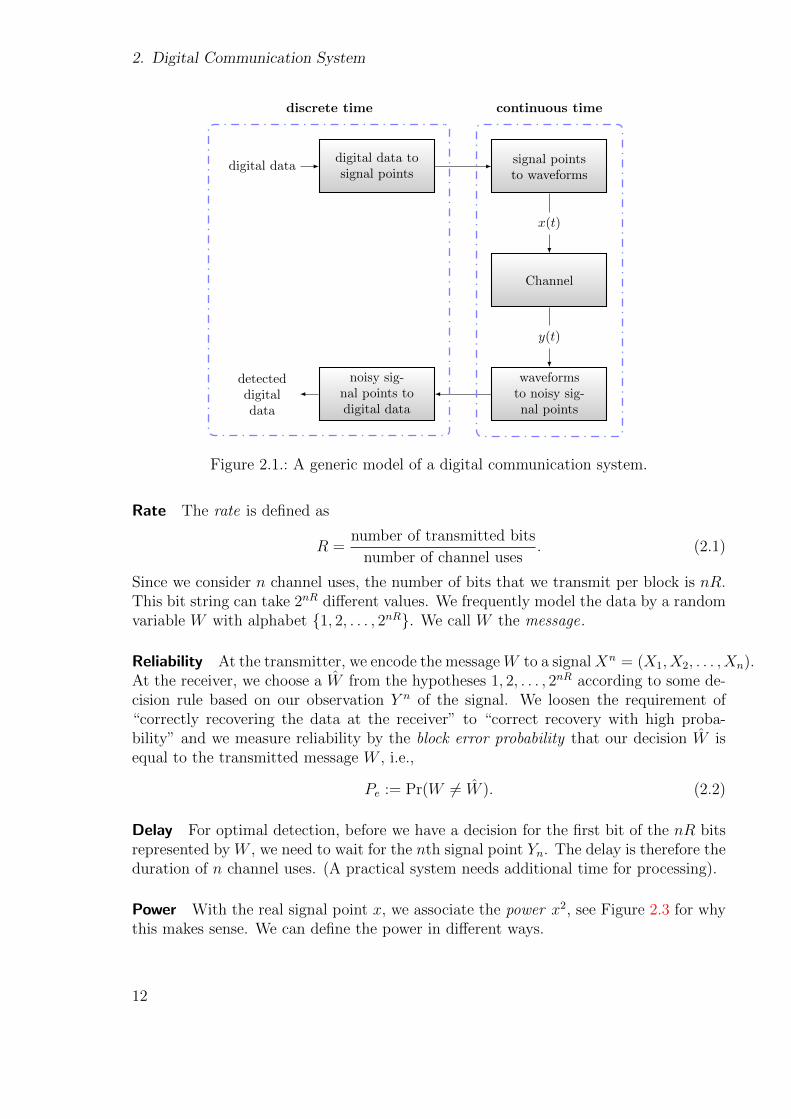
A simple model of a digital transmission system is shown in Figure 2.1. At the trans-mitter, data bits are mapped to a sequence of signal points, which are then transformedinto a waveform. The channel distorts the transmitted waveform. At the receiver, thereceived waveform is transformed into a sequence of noisy signal points. This sequenceis then transformed into a sequence of detected data bit. The signal points and the noisysignal points, respectively, form the interface between continuous-time and discrete-timesignal processing in the communication system. Modeling and analysis of the continuous-time part and the conversion between discrete-time signals and continuous-time signalsis discussed in many textbooks. For example, an introduction to the representation ofcontinuous waveforms is given in [2, Chapter 4]. The conversion of continuous waveformsinto discrete-time sequences is discussed in [6, Chapter 4].

We treat the time-continuous part of the digital transmission system as part of achannel with discrete-time input (the signal points) and discrete-time output (the noisysignal points).

2.2. Figures of Merit

To design a transmission system, we must identify the figures of merit that we areinterested in. Common properties of interest are as follows.

• Rate: We want to transmit the data over the channel as fast as possible.

• Reliability: We want to recover the transmitted data correctly at the receiver.

• Delay: We want to be “real-time”.

• Power: We want to use as low power as possible/we want to comply with legalpower restrictions.

• Energy: We want to spend a small amount of energy to transmit a data packet.

To quantify the properties of interest, we consider block-based transmission, i.e., wejointly consider n consecutive channel uses. See Figure 2.2 for an illustration. Theparameter n is called the block length or number of channel uses. Rate, reliability, delay,power, and energy can now be quantified as follows.

11


digital datadigital data tosignal points

signal pointsto waveforms

x(t)

Channel

y(t)

detecteddigitaldata

noisy sig-nal points todigital data

waveformsto noisy sig-nal points

discrete time continuous time

Figure 2.1.: A generic model of a digital communication system.

Rate The rate is defined as

R =number of transmitted bits

number of channel uses. (2.1)

Since we consider n channel uses, the number of bits that we transmit per block is nR.This bit string can take 2nR different values. We frequently model the data by a randomvariable W with alphabet 1, 2, . . . , 2nR. We call W the message.

Reliability At the transmitter, we encode the messageW to a signalXn = (X1, X2, . . . , Xn).At the receiver, we choose a W from the hypotheses 1, 2, . . . , 2nR according to some de-cision rule based on our observation Y n of the signal. We loosen the requirement of“correctly recovering the data at the receiver” to “correct recovery with high proba-bility” and we measure reliability by the block error probability that our decision W isequal to the transmitted message W , i.e.,

Pe := Pr(W 6= W ). (2.2)

Delay For optimal detection, before we have a decision for the first bit of the nR bitsrepresented by W , we need to wait for the nth signal point Yn. The delay is therefore theduration of n channel uses. (A practical system needs additional time for processing).

Power With the real signal point x, we associate the power x2, see Figure 2.3 for whythis makes sense. We can define the power in different ways.

12

2.2. Figures of Merit

W Encoder X1X2 . . . Xn

Y1Y2 . . . Yn

Channel

DecoderW

Figure 2.2.: Block-based transmission over a discrete-time channel. The message W cantake the values 1, 2, . . . , 2nR, which can be represented by nR bits. Themessage W is encoded to a discrete signal Xn = xn(W ). The decoderdetects the message from the observed channel output Y n and outputs adecision W .

1Ω x Volt

Figure 2.3.: We can think of the input x as the voltage over a unit resistance. Sincepower = current × voltage, we have the power = x2/1 Watts by Ohm’s law.

• We say a system has peak power at most P if

x2 ≤ P, for each transmitted signal point x. (2.3)

• A system has per-block power at most P if∑ni=1 x

2i

n≤ P, for each transmitted signal xn. (2.4)

• A system has average power at most P if the average per-block-power is upperbounded by P, i.e., if

E [∑n

i=1 X2i ]

n≤ P. (2.5)

Note that the three power constraints are ordered, namely (2.3) implies (2.4), and (2.4)implies (2.5). In particular, requiring the per-block power to be smaller than P is morerestrictive than requiring an average power to be smaller than P. The most importantnotion of power is the average power. In the following, we will use the terms “power”and “average power” interchangeably.

13


Example 2.1 (BPSK). Suppose the transmitted signal points take one of the twovalues −A,A. This modulation scheme is called binary phase shift keying (BPSK).For BPSK the peak power, the per-block power, and the average power are all equalto A2, independent of the block length n.

Example 2.2 (4-ASK). Suppose the transmitted signal points take on values in

−3A,−A,A, 3A

with equal probability. This modulation scheme is usually called amplitude shiftkeying (ASK) although both amplitude and phase are modulated. The peak powerof this scheme is 9A2. The signal with highest per-block power is the one that hasall signal points equal to 3A or −3A. The average power of the considered schemeis

1

2A2 +

1

29A2 = 5A2 (2.6)

which is significantly less than the peak power and the highest per-block power.

Example 2.3 (Block-Based Transmission). Suppose the block length is n = 4 andthe signal points take values in a 3-ASK constellation X = −1, 0, 1. Supposefurther that the message W is uniformly distributed on W = 1, 2, . . . , 8 and thatthe encoder f : W → C ⊆ −1, 0, 1n is given by

1 7→ (−1, 0, 0, 1)

2 7→ (−1, 1, 0, 0)

3 7→ (0,−1, 0, 1)

4 7→ (0, 0,−1, 1)

5 7→ (0, 1,−1, 0)

6 7→ (0, 1, 0,−1)

7 7→ (1,−1, 0, 0)

8 7→ (1, 0, 0,−1).

The rate of this scheme is

R =3

4

[bits

channel use

]. (2.7)

The peak power is 1, the per-block power is 0.5 for each code word in C and con-sequently, the average power is also equal to 1

2. Let X1X2X3X4 := f(W ) be the

14

2.3. Data Interface

transmitted signal. The distribution of Xi, i = 1, 2, 3, 4 is

PXi(−1) = PXi(1) =1

4, PXi(0) =

1

2. (2.8)

Energy We quantify energy by Eb, which is the energy that we spend to transmit onebit of data. We have

Eb =energy

bit=

energy

channel use· channel use

bit=

power

rate=

P

R. (2.9)

2.3. Data Interface

The data to be transmitted is often modelled by a sequence of independent and uniformlydistributed bits. For block-based transmission, this binary stream is partitioned intochunks of nR bits each, which represent the messages that we transmit per block. Eachmessage is usually modelled as uniformly distributed. This is a good model for manykinds of digital data, especially when the data is in a compressed format such as .zipor .mp3. Separating the real world data from the digital transmission system by abinary interface is often referred to by source/channel separation. This principle allowsto separately design source encoders (i.e., compression algorithms) and transmissionsystems. The separation of source encoding and transmission implies virtually no lossin performance, see for example [4, Section 7.13] and [2, Chapter 1].

2.4. Capacity

We now want to relate reliability, power, and rate. Consider the transmission system inFigure 2.2. It consists of an encoder that maps the nR bit message W to the signal Xn

and a decoder that maps the received signal Y n to a decision W .

Definition 1 (Achievable). We say the rate R is achievable under the power constraintP, if for each ε > 0 and a large enough block length n(ε), there exists a transmission sys-tem with 2n(ε)R code words with an average power smaller or equal to P and a probabilityof error smaller than ε, i.e.,

Pe = Pr(W 6= W ) < ε.

The capacity of a channel is the supremum of all achievable rates. For some chan-nels, the channel capacity can be calculated in closed form. For example, for discretememoryless channels with input-output relation

PY n|Xn(bn|xn) =n∏i=1

PY |X(bi|ai), an ∈ X n, bn ∈ Yn (2.10)

15


the capacity is

maxX : E(X2)≤P

I(X;Y ) (2.11)

where I(X;Y ) is the mutual information defined in Appendix C.5. The capacity result(2.11) also holds for continuous output memoryless channels with discrete input andwith continuous input. In Section 3.4, we discuss the capacity formula of the memorylessAWGN channel.

An important step in the derivation of this result is to show that for any δ > 0, thevalue I(X;Y )− δ is an achievable rate in the sense of Definition 1. This suggests to callI(X;Y ) an approachable rate rather than an achievable rate, since the requirements ofDefinition 1 are only verified for I(X;Y ) − δ, not for I(X;Y ). In this work, we followthe common terminology ignoring this subtlety and call I(X;Y ) an achievable rate, inconsistency with literature.

For a large class of channels, including many practical channels, achievable rates canbe estimated that provide a lower bound on the channel capacity. Achievability schemesoperating close to capacity is the main topic of theses notes and chapters 7–10 developsuch schemes in detail.

2.4.1. Channel Coding Converse for Memoryless Channels

We next state a converse result, namely that above a certain threshold, reliable commu-nication is impossible. The derivation of converse results is in general involved; here, weonly consider the special case of memoryless channels. Our goal is to attach a first op-erational meaning to the mutual information, which we will then study in detail for theAWGN in the chapters 3–5 and which will serve as a guidance for transmitter design inChapter 6. The statement and proof of the converse result uses basic information mea-sures, namely the entropy H(X) of a discrete random variable X, the binary entropyfunction H2(P ) of a probability P , and the differential entropy h(Y ) of a continuousrandom variable Y . The definitions and basic properties of these information measuresare stated in Appendix C.

Theorem 1 (Channel Coding Converse). Consider a transmission system with blocklength n. The message W can take the values 1, 2, . . . , 2nR. The code word Xn = xn(W )is transmitted over a memoryless channel pY |X . If

H(W )

n>

∑ni=1 I(Xi;Yi)

n(2.12)

then the probability of error Pe = Pr(W 6= W ) is bounded away from zero.

16

2.5. Problems

Proof. We have

H2(Pe) + Pe log2(2nR − 1)(a)

≥ H(W |W )

= H(W )− I(W ; W )

(b)

≥ H(W )− I(Xn;Y n)

(c)= H(W )−

[h(Y n)−

n∑i=1

h(Yi|Xi)]

(d)

≥ H(W )−n∑i=1

[h(Yi)− h(Yi|Xi)

]= H(W )−

n∑i=1

I(Xi;Yi)

where (a) follows by Fano’s inequality (C.18), (b) by the data-processing inequality(C.41), (c) follows because the channel is memoryless and (d) follows by the independencebound on entropy (C.12). Dividing by n, we have

H(W )

n−∑n

i=1 I(Xi;Yi)

n≤ H2(Pe)

n+ Pe

log2(2nR − 1)

n≤ H2(Pe) + PeR.

That is, if H(W )/n >∑ni=1 I(Xi;Yi)

nthen Pe is bounded away from zero.

2.5. Problems

Problem 2.1. For the transmission scheme of Example 2.3, calculate the direct currentthat results from one block transmission.Problem 2.2. Let X1, X2, . . . , Xn be distributed according to the joint distribution PXn

(the Xi are possibly stochastically dependent). Show that

E [∑n

i=1X2i ]

n=

∑ni=1 E[X2

i ]

n. (2.13)

17

3. AWGN Channel

3.1. Summary

• The discrete time AWGN channel is

Y = X + Z. (3.1)

• Y,X,Z are channel output, channel input, and noise, respectively.

• The input X and noise Z are stochastically independent.

• The noise Z is zero mean Gaussian with variance σ2.

• A real-valued random variable X has power E(X2).

• The SNR is snr = input powernoise power

.

• SNR in dB is 10 log10 snr.

• The capacity of the AWGN channel is

C(snr) =1

2log2(1 + snr)

[bits

channel use

](3.2)

inverse: snr = C−1(R) = 22R − 1. (3.3)

• C(snr) is plotted in Figure 3.1.

• Phase transition at capacity: For a fixed snr∗, reliable communication at a rate R ispossible, if R < C(snr∗), and impossible, if R > C(snr∗). For a fixed rate R∗, reliablecommunication is possible if snr > C−1(R∗) and impossible, if snr < C−1(R∗).

3.2. Channel Model

At each time instant i, we describe the discrete time memoryless AWGN channel by theinput-output relation

Yi = xi + Zi. (3.4)

The noisy signal point Yi is the sum of the signal point xi and the noise Zi. Thenoise random variables Zi, i ∈ Z (Z denotes the set of integers) are independent and

19

3. AWGN Channel

identically distributed (iid) according to a Gaussian density with zero mean and varianceσ2, i.e., the Zi have the probability density function (pdf)

pZ(z) =1√

2πσ2e−

z2

2σ2 , z ∈ R. (3.5)

The relation (3.4) can equivalently be represented by the conditional output pdf

pY |X(y|x) = pZ(y − x). (3.6)

We model the channel input as a random variable X that is stochastically independentof the noise Z.

Discussion Using the model (3.4) to abstract the continuous-time part of the digitaltransmission system can be justified in several ways. An in-depth treatment can befound in [3, Chapter 8]. In [7], it is shown with mathematical rigor that, under certainconditions, the Yi form a sufficient statistics, i.e., all the information about Xi that iscontained in the continuous-time received waveform is also contained in the discrete-time noisy signal point Yi. This approach explicitly models the noise that gets added tothe waveform as white Gaussian noise. However, we can only “see” the noise throughfilters. A second approach to justify (3.4) is therefore to build the digital transmissionsystem, perform a measurement campaign, and to find a reasonable statistical modelfor the noise sequence Zi = Yi −Xi, where Xi is chosen at the transmitter and knownand where Yi is measured at the receiver. For instance, this approach was used in [8] toderive a channel model for ultra-wideband wireless communication. Finding the “true”channel description is often difficult. A third approach is to design systems that operateas if the channel would be an AWGN channel. This leads to a mismatch between theactual channel and the channel assumed by the transceiver. The mismatched approachis an effective method for designing communication systems for practical channels andwe use it in the chapters 7–11. We use “the channel assumed by the transceiver” and“decoding metric” as synonyms.

3.3. Signal-to-Noise Ratio and Eb/N0

SNR Consider the AWGN channel model

Y = X + Z (3.7)

where Z is Gaussian noise with variance σ2. We scale (3.7) by some constant κ. Theresulting input-output relation is

κ · Y︸︷︷︸=:Y

= κ ·X︸︷︷︸=:X

+κ · Z︸︷︷︸=:Z

(3.8)

which gives us a modified channel model

Y = X + Z. (3.9)

20

3.4. Capacity

Suppose the power of X is E(X2) = P. The power of X is then κ2P, so the transmittedsignal in (3.9) has a power that is different from the power of the transmitted signal in(3.7). The power of the noise has also changed, namely from σ2 in (3.7) to κ2σ2 in (3.9).What remains constant under scaling is the SNR, which is defined as

snr :=signal power

noise power. (3.10)

The SNR is unitless, so if the signal power is P Watts and the noise power is σ2 Watts,then the SNR is P/σ2 (unitless). The SNR is often expressed in decibel (dB), which isdefined as

SNR in dB = snrdB = 10 log10 snr. (3.11)

Eb/N0 The relation of signal power and noise power can alternatively be expressed bythe Eb/N0. As defined in (2.9), Eb is the energy we spend to transmit one message bit .N0 is the noise variance per two dimensions, i.e., if the noise variance per channel use isσ2, then N0 = 2σ2. We can express Eb/N0 in terms of SNR by

Eb/N0 =P

R· 1

2σ2=

P

σ2· 1

2R=

snr

2R(3.12)

where R is the rate as defined in (2.1). In decibel, Eb/N0 is

Eb/N0 in dB = 10 log10(Eb/N0). (3.13)

3.4. Capacity

Recall the capacity result (2.11), which says that for a power constraint P, the capacityof a memoryless channel is

maxX : E(X2)≤P

I(X;Y ). (3.14)

We denote the maximizing input random variable by X∗. For the AWGN channel, byProblem 3.3, X∗ has a Gaussian density with zero mean and variance P.

Theorem 2 (AWGN Capacity). For the AWGN channel with power constraint P andnoise variance σ2, the capacity-power function is

C(P/σ2) =1

2log(1 + P/σ2). (3.15)

In other words, we have the following result.

1. (Converse) No rate R > C(P/σ2) is achievable by a system with average power lessor equal to P.

2. (Achievability) Any rate R < C(P/σ2) is achievable by a system with average powerP.

We provide a plot of the capacity-power function in Figure 3.1.

21

3. AWGN Channel

−10 −5 0 5 10 15 200

0.5

1

1.5

2

2.5

3

3.5

SNR, Eb/N0 in dB

capacityin

bitsper

channel

use

12 log2(1 +

Pσ2 ) versus Eb/N0

12 log2(1 +

Pσ2 ) versus SNR

Figure 3.1.: The capacity-power function.

3.5. Problems

Problem 3.1. Let X and Z be stochastically independent Gaussian random variableswith means µ1, µ2 and variances σ2

1, σ22. Show that Y = X + Z is zero mean Gaussian

with mean µ1 + µ2 and variance σ21 + σ2

2.Hint: Use that for two independent real-valued random variables pX , pZ , the pdf of thesum is given by the convolution of pX with pZ .Problem 3.2. Let X have density pX with mean µ and variance σ2. Let Y be Gaussianwith the same mean µ and variance σ2. Show that h(Y ) ≥ h(X) with equality if andonly if X has the same density as Y , i.e., if X is also Gaussian.Hint: You can use the information inequality (C.21) in your derivation.Problem 3.3. Consider the AWGN channel Y = X + Z, where Z is Gaussian withzero mean and variance σ2, where X and Z are stochastically independent, and whereE(X2) ≤ P. Show that

I(X;Y ) ≤ 1

2log(1 + P/σ2). (3.16)

For which pdf pX is the maximum achieved?Hint: You can use Problem 3.1 and Problem 3.2 in your derivation.Problem 3.4. Consider two (SNR,rate) operating points (snr1,C(snr1)) and (snr2,C(snr2))on the power-rate function.

1. Investigate the dependence of the SNR gap in dB on the rate gap for high SNR,

22

3.5. Problems

i.e., to which value does the ratio

10 log10(snr2)− 10 log10(snr1)

C(snr2)− C(snr1)(3.17)

converge for snr2, snr1 →∞?

2. To which value does (3.17) converge for P2,P1 → 0?

3. Answer the questions 1. and 2. when Eb/N0 in dB is used in (3.17) instead of theSNR in dB.

Problem 3.5.

1. To which value does Eb/N0 in dB converge when the SNR approaches −∞?

2. What is the minimum energy we need to transmit one bit reliably over the AWGNchannel?

3. How long will the transmission of one bit with minimum energy take?

23

4. Shaping Gaps for AWGN

For the AWGN channel, we have

Y = X + Z (4.1)

with noise variance σ2 and input power constraint P. We want to characterize the loss ofmutual information of an input X and an output Y that results from not using Gaussianinput. We consider the following three situations.

1. The input is not Gaussian.

2. The input is continuous and uniformly distributed.

3. The input is discrete and uniformly distributed.

See Figure 4.1 for an illustration of the considered input distributions.

4.1. Summary

• The ASK constellation with M signal points (M -ASK) is

X = ±1,±3, . . . ,±(M − 1). (4.2)

• Let X be uniformly distributed on X .

• The channel input is ∆X where ∆ is a positive real number; the input power is∆2 E(X2).

• An achievable rate is

I(X;Y ) = I(X; ∆X + Z). (4.3)

• Achievable rates for 2m-ASK are plotted in Figure 4.3. Observations:

– Ungerboeck’s rule of thumb [9]: The 2m-ASK curves stay close to capacityfor rates smaller than m− 1.

– The 2m-ASK curves saturate at m bits for large SNR.

– Shaping gap: with increasing m, a gap to capacity becomes apparent. Thegap is caused by the uniform input distribution over the set of permittedsignal points. The gap converges to 1.53 dB, asymptotically in the ASKconstellation size and the SNR.

25


x

pX∗

pXu

PXM

Figure 4.1.: The Gaussian density pX∗ , the uniform density pXu and the uniform distri-bution PXM on a discrete M -ASK constellation. The densities pX∗ , pXu andthe distribution PXM have the same variance.

4.2. Non-Gaussian Input

By Problem 3.3, the capacity-achieving density pX∗ of the AWGN channel with powerconstraint P is zero mean Gaussian with variance P. When pX∗ is used for the channelinput, the resulting output Y ∗ = X∗ + Z is zero mean Gaussian with variance P + σ2,see Problem 3.1. Let now X be a channel input, discrete or continuous, with zero meanand variance P. We expand the mutual information as

I(X;Y ) = h(Y )− h(Y |X). (4.4)

For the conditional differential entropy, we have

h(Y |X)(a)= h(Y −X|X) (4.5)

= h(Z|X) (4.6)

(b)= h(Z) =

1

2log2(2πeσ2) (4.7)

where (a) follows by (C.9) and where (b) follows because X and Z are independent.

Remark 1. We calculated the right-hand side of (4.7) using the definition of differentialentropy (C.5). Since σ2 = E(Z2) is the noise power, it should have the unit Watts.However, the argument of the logarithm must be unitless. In Problem 4.11, we providean alternative definition of differential entropy, which works with units. Using the alter-native differential entropy definition does not alter the results presented in this chapter.

By (4.7), the term h(Y |X) does not depend on how the input X is distributed. How-ever, the differential entropy h(Y ) does depend on the distribution of X. For continuousX, the density of Y is given by

pY (y) =

∫ ∞−∞

pX(x)pZ(y − x) dx = (pX ? pZ)(y) (4.8)

that is, pY is the convolution of pX and pZ . If X is discrete, the density pY is given by

pY (y) =∑x∈X

PX(x)pZ(y − x). (4.9)

26

4.3. Uniform Continuous Input

The differential entropy h(Y ) is a functional of the density pY and it is in general difficultto derive closed-form expressions. We next write h(Y ) as

h(Y )(a)= h(Y ∗)− D(pY ‖pY ∗) (4.10)

where (a) is shown in Problem 4.4. We can now write I(X;Y ) as

I(X;Y ) = h(Y )− h(Y |X) (4.11)

(a)= h(Y )− h(Z) (4.12)

(b)= h(Y ∗)− D(pY ‖pY ∗)− h(Z) (4.13)

(c)= [h(Y ∗)− h(Y ∗|X∗)]− D(pY ‖pY ∗) (4.14)

= C(P/σ2)− D(pY ‖pY ∗) (4.15)

where we used (4.7) in (a) and (c) and (4.10) in (b). We make the following twoobservations.

• The loss of mutual information when using X instead of X∗ is the informationaldivergence D(pY ‖pY ∗) between the resulting output distributions.

• The loss can be small even if X differs significantly from X∗ as long as the resultingoutput distribution pY is similar to pY ∗ . See also Problem 4.6.

We next consider two constraints on the input. First, we let X be uniformly distributedon a continuous finite interval, and second, we let X be uniformly distributed on adiscrete ASK constellation.

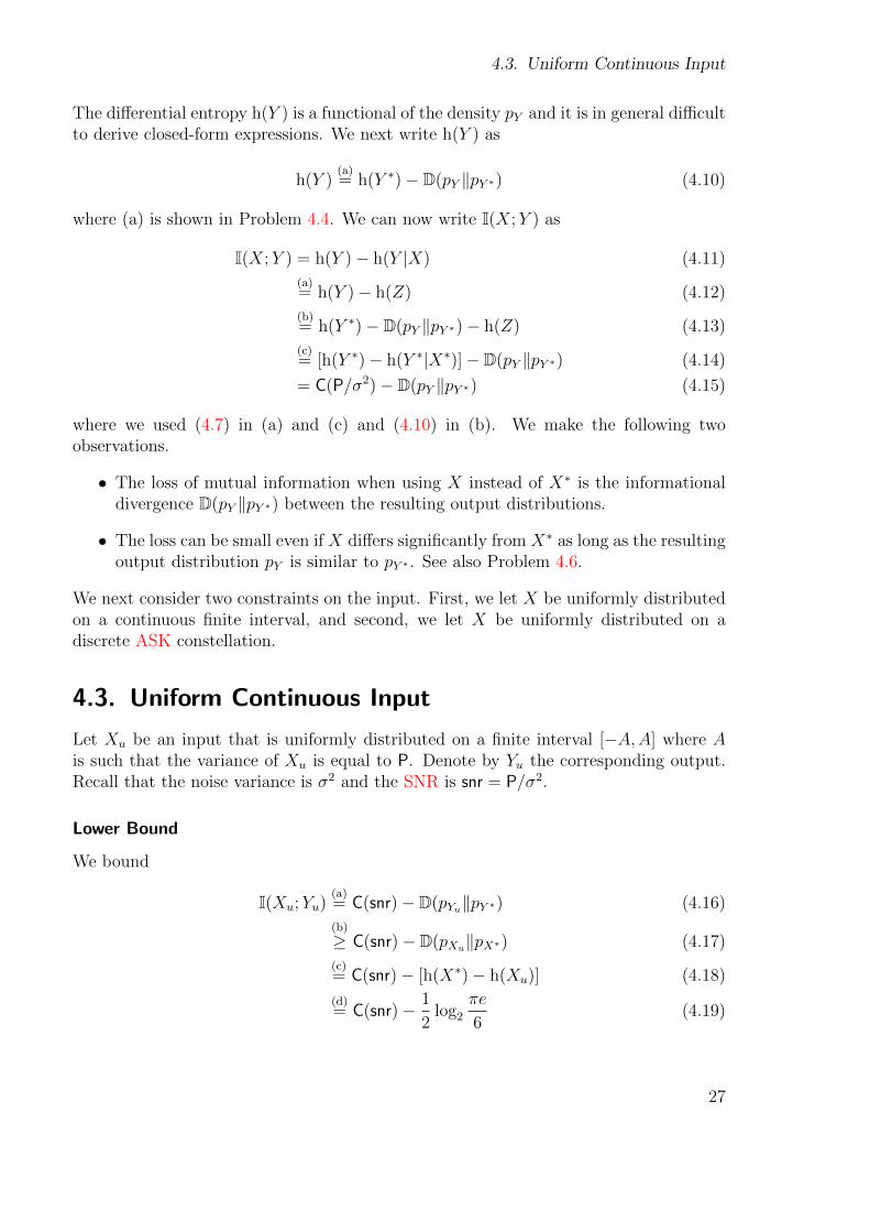
4.3. Uniform Continuous Input

Let Xu be an input that is uniformly distributed on a finite interval [−A,A] where Ais such that the variance of Xu is equal to P. Denote by Yu the corresponding output.Recall that the noise variance is σ2 and the SNR is snr = P/σ2.

Lower Bound

We bound

I(Xu;Yu)(a)= C(snr)− D(pYu‖pY ∗) (4.16)

(b)

≥ C(snr)− D(pXu‖pX∗) (4.17)

(c)= C(snr)− [h(X∗)− h(Xu)] (4.18)

(d)= C(snr)− 1

2log2

πe

6(4.19)

27


0 5 10 15 20 25 30 350

1

2

3

4

5

SNR in dB

bitsper

channel

use

C(P/σ2)

C(P/σ2)− 12 log2

πe6

Figure 4.2.: The dashed line shows the lower bound (4.19) for continuous uniformlydistributed input.

where (a) follows by (4.15), where (b) follows by Problem 4.6, where (c) follows byProblem 4.4, and where (d) follows by Problem 4.5. The inequality D(pXu‖pX∗) ≥D(pYu‖pY ∗) that we used in (b) is a data processing inequality, see [5, Lemma 3.11]. Wemake the following observation.

• The loss of mutual information because of a uniform input density is at most12

log2πe6

independent of the SNR snr. The value 12

log2πe6

is sometimes called theshaping gap.

We can also express (4.19) as

I(Xu;Yu) = h(Xu)− h(Xu|Yu) (4.20)

≥ h(Xu)−1

2log2

(2πe

P

1 + P/σ2

)(4.21)

which shows that the conditional entropy of Xu is bounded from above by

h(Xu|Yu) ≤1

2log2

(2πe

P

1 + P/σ2

). (4.22)

Upper Bound

We next want to show that the shaping gap (4.19) is tight, i.e., that for large SNR, thelower bound (4.19) holds with equality. To this end, we will derive an upper bound for

28

4.4. Finite Signal Constellations

I(Xu;Yu) that approaches (4.19) from above when the SNR approaches infinity. Notethat because Xu is uniformly distributed on [−A,A], it fulfills the peak-power constraint

|Xu| ≤ A. (4.23)

We can thus use the following mutual information upper-bound for input with peakpower A:

supp pX ⊆ [−A,A]⇒ I(X;Y ) ≤ log2

(1 +

√2A2

πeσ2

). (4.24)

This bound is stated in [10] and proven in [11], see also [12]. Note that the bound holdsalso for non-uniformly distributed input.

Since E(X2u) = A2/3 = P, we have A2 = 3P. We can now bound the shaping gap from

below by

C(P/σ2)− I(Xu;Yu) ≥ C(P/σ2)− log2

(1 +

√6P

πeσ2

)(4.25)

=1

2log2(1 + snr)− 1

2log2

(1 + 2

√6snr

πe+

6snr

πe

)(4.26)

=1

2log2

1 + snr

1 + 2√

6snrπe

+ 6snrπe

(4.27)

=1

2log2

1snr

+ 1

1snr

+ 2√

6πesnr

+ 6πe

(4.28)

snr→∞→ 1

2log2

πe

6. (4.29)

Thus, asymptotically in the SNR, the shaping gap lower bound is tight, i.e., it approachesthe upper bound 1

2log2

πe6

. Summarizing, we have

C(snr)− I(Xu;Yu) ≤1

2log2

πe

6(for any SNR) (4.30)

limsnr→∞

C(snr)− I(Xu;Yu) =1

2log2

πe

6. (4.31)

4.4. Finite Signal Constellations

For notational convenience, we deviate in this section from our standard notation (4.2)for M -ASK constellations and define

X = ±∆,±3∆, . . . ,±(M − 1)∆ (4.32)

29


so that the channel input is X (instead of X∆). Let XM be uniformly distributed onX . The resulting power is

P = E(X2M) = ∆2M

2 − 1

3(4.33)

see Table 4.1.

Theorem 3 (Uniform Discrete Input Bound). The mutual information achieved by XM

is lower bounded by

I(XM ;YM) ≥ 1

2log2

(12P

M2

M2 − 1

)− 1

2log2

[2πe

(P

M2 − 1+

P

1 + P/σ2

)](4.34)

> C(snr)− 1

2log2

πe

6− 1

2log2

[1 +

(2C(snr)

M

)2]

(4.35)

where snr = P/σ2.

Proof. We prove the theorem in Section 4.5.

Our input XM is suboptimal in two ways. First, it is restricted to the set X ofM equidistant points, and second, XM is distributed uniformly on X . Because of ourresult from Section 4.3 for uniform inputs, the mutual information is bounded awayfrom capacity by 1

2log2

πe6≈ 0.255 bits independent of how large we choose M . Let’s

see how M needs to scale with C(snr) so that the resulting mutual information is withina constant gap of capacity. To keep the finite constellation loss within the order of thedistribution loss of 0.255 bits, we calculate

1

2log2

[1 +

(2C(snr)

M

)2]≤ log2 e

2

(1

M · 2−C(snr)

)2

=1

4(4.36)

⇔M = 2C(snr)+ 12

+ 12

log2 log2 e (4.37)

where we used log2 x = log2(e) log(x) ≤ log2(e)(x − 1). We conclude from (4.37) thatthe mutual information is within 0.5 bit of capacity if

log2M ≈ C(snr) + 0.77. (4.38)

This condition can be confirmed in Figure 4.3, where we display rate curves and boundsfor ASK constellations with uniformly distributed input.

4.5. Proof of Uniform Discrete Input Bound

We can expand mutual information in two ways, namely

I(XM ;YM) = h(YM)− h(YM |XM) = H(XM)−H(XM |YM) (4.39)

30


0 5 10 15 20 25 300

1

2

3

4

5

SNR in dB

bitsper

channel

use

C(P/σ2)

C(P/σ2)− 12 log2

πe6

16-ASK

8-ASK

4-ASK

BPSK

Figure 4.3.: The dotted curves show the bound (4.35) from Theorem 3. The gap betweenthe dotted curves and the capacity-power function confirms the condition(4.38). The dashed line shows the lower bound (4.19) for continuous uni-formly distributed input. Note that for low SNR, the rate curves for ASKare close to the capacity-power function, while for high SNR, the dashedcurve becomes a tight lower bound, i.e., for high SNR and large ASK con-stellations, the shaping gap of 1

2log2

πe6

becomes apparent.

31


X

U

+ XM +

Z

YM

Figure 4.4.: U is uniformly distributed on [−∆,∆] and X is uniformly distributed on[−∆M,∆M ].

where we know

h(YM |XM) = h(Z) =1

2log2(2πeσ2) (4.40)

H(XM) = log2M (4.41)

but we have no insightful expressions for h(YM) and H(XM |YM). We want to lower boundI(XM ;YM), so we can either lower bound h(YM) or we can upper bound H(XM |YM).Following [13], we opt for upper bounding H(XM |YM). We do this in two steps:

1. We introduce an auxiliary continuous random variable X that is a function of XM ,so that I(XM ;YM) ≥ I(X;YM) by the data processing inequality (C.41).

2. We upper bound h(X|YM) by using a conditional version of the information in-equality (C.21).

Step 1: Auxiliary Continuous Input X The random variable XM is discrete. To makeour life easier, we first introduce an auxiliary random variable. Let U be continuous anduniformly distributed on [−∆,∆) and define

X := XM + U. (4.42)

We provide an illustration in Figure 4.4. From the definitions of XM and U , it followsthat X is continuous and uniformly distributed on [−∆M,∆M). Since X XM YMform a Markov chain, we have by the data processing inequality (C.41)

I(XM ;YM) ≥ I(X;YM) (4.43)

= h(X)− h(X|YM). (4.44)

For the differential entropy h(X), we have

h(X) = log2(2M∆) =1

2log2(4M2∆2) =

1

2log2

12M2P

M2 − 1(4.45)

where we used Table 4.1. Inserting the right-hand side of (4.45) in (4.44), we have

I(XM ;YM) ≥ 1

2log2

12M2P

M2 − 1− h(X|YM). (4.46)

In the next paragraph, we replace h(X|YM) by an insightful upper bound.

32


E(X2M) = P = (M2−1)∆2

3

E(U2) = ∆2

3

E(X2) = (M∆)2

3

Table 4.1.: Powers of XM , U , and X as derived in Problem 4.3.

Step 2: Bounding h(X|YM). By Problem 4.7, we have

h(X|YM) = E[− log2 pX|YM (X|YM)] (4.47)

≤ E[− log2 q(X|YM)] (4.48)

for any q(·|·) with the property that q(·|y) is a density on R for every y ∈ R. We choosea Gaussian density with mean ky and variance s2, i.e., we choose

q(x|y; k, s2) :=1√2πs

exp

[−(x− ky)2

2s2

]. (4.49)

This gives

h(X|YM) ≤ log2(e)

(1

2ln(2πs2) +

1

2s2E[(X − kYM)2]

). (4.50)

We calculate the expectation.

E[(X − kYM)2] = E[(XM + U − k(XM + Z))2] (4.51)

= E[((1− k)XM + U − kZ)2] (4.52)

(a)= P +

∆2

3− 2kP + k2(P + σ2) (4.53)

where the reader is asked to verify (a) in Problem 4.8. We can now write the bound forthe conditional entropy of X as

h(X|YM) ≤ log2(e)

(1

2ln(2πs2) +

1

2s2

[P +

∆2

3− 2kP + k2(P + σ2)

]). (4.54)

In Problem 4.8, we minimize this expression over the parameters k and s2. The solutionis k = P

P+σ2 and s2 = ∆2

3+ P

1+P/σ2 and the minimized bound is

h(X|YM) ≤ 1

2log2

[2πe

(∆2

3+

P

1 + P/σ2

)]. (4.55)

Remark 2. We can express ∆ in terms of M and P, namely

∆2 =3P

M2 − 1. (4.56)

33


Thus, we have

h(X|YM) ≤ 1

2log2

[2πe

(P

M2 − 1+

P

1 + P/σ2

)](4.57)

M→∞→ ≤ 1

2log2

[2πe

P

1 + P/σ2

]. (4.58)

Thus, as the number of signal points approaches infinity, our upper bound on h(X|YM)approaches our upper bound (4.22) on h(Xu|Yu).Remark 3. We can show that we have equality in (4.43), i.e., I(XM ;YM) = I(X;YM).The reason is that XM is a deterministic function of X. Formally, note that U = X−XM

and Z = YM −XM and by definition X = XM +U and YM = XM +Z. Thus, by (C.40),we have

I(X;YM |XM) = I(X, U ;YM , Z|XM) = I(U ;Z|XM)(a)= 0 (4.59)

where (a) follows because XM , Z, U are stochastically independent. Thus, we have

I(X;YM)(a)= I(X,XM ;YM) (4.60)

(b)= I(XM ;YM) + I(X;YM |XM) (4.61)

(c)= I(XM ;YM) (4.62)

where (a) follows by (C.40) (XM is a function of X), where (b) follows by (C.39), andwhere (c) follows by (4.59). This proves the equality.

4.6. Problems

Problem 4.1. Derive (4.8) by using the definitions of density (B.1) and expectation(B.4) and the law of total probability (B.5). Hint: Show that

Pr(Y ≤ y) =

∫ y

−∞

∫ ∞−∞

pX(x)pZ(τ − x) dx dτ. (4.63)

Problem 4.2. Show that if the channel input X takes values in an M -ASK constellation,then the mutual information of channel input X and channel output Y is upper boundedby log2M .Problem 4.3. Let X be uniformly distributed on [−A,A]. Show that

Var(X) =A2

3. (4.64)

Problem 4.4. Let X be some continuous random variable with zero mean and varianceP. Let X ′ be zero mean Gaussian with variance P. Show that

h(X ′)− h(X) = D(pX‖pX′). (4.65)

Problem 4.5. LetX andX ′ be continuous random variables with zero mean and varianceP. Suppose X is distributed uniformly on [−d, d] and let X ′ be Gaussian.

34

4.6. Problems

1. Show that

h(X) =1

2log2(12P) (4.66)

h(X ′) =1

2log2(2πeP). (4.67)

2. Show that

h(X ′)− h(X) =1

2log2

πe

6. (4.68)

Problem 4.6. Let pX and pX′ be two densities defined on X . Let pY |Z be a conditionaldensity where Z takes values in X . Define

pXY (a, b) = pX(a)pY |Z(b|a) (4.69)

pX′Y ′(a, b) = pX′(a)pY |Z(b|a) (4.70)

Show that

D(pY ‖pY ′) ≤ D(pX‖pX′). (4.71)

Hint: Use the chain rule of informational divergence (C.25) and the information inequal-ity (C.21).Problem 4.7.

1. Let pX be a density and let q be some other density with q(a) = 0 ⇒ pX(a) = 0,i.e., supp pX ⊆ supp q. Show that

h(X) = E[− log2 pX(X)] ≤ E[− log2 q(X)] (4.72)

where all expectations are taken with respect to pX .

2. Let now pXY = pXpY |X be a joint density and for each x ∈ supp pX , let q(·|x) bea density on R with supp pY |X(·|x) ⊆ supp q(·|x). Use the result from 1. to showthat

h(Y |X) = E[− log2 pY |X(Y |X)] ≤ E[− log2 q(Y |X)]. (4.73)

Problem 4.8. Verify (4.53), (4.55), and (4.35).Problem 4.9. Use the bounding technique from Problem (4.7) with the Ansatz (4.49)for an alternative derivation of the bound (4.19).Problem 4.10. Show that the gap in SNR in dB between the bound (4.19) and thecapacity-power function approaches approximately 1.53 dB when the SNR goes to in-finity.Problem 4.11. Let Z be zero mean Gaussian with variance σ2 with unit Watts, i.e., Zhas unit

√Watt.

35


1. Show that if the variance σ2 has unit Watts, then the density pZ has unit 1/√

Watt.

2. Consider the probability Pr(a ≤ Z ≤ b) =∫ bapZ(τ) dτ . Verify that the probability

is unitless if dτ has the same unit as Z.

3. Define differential entropy as alternative to (C.5) by

hr(Z) = E [− log2[pZ(Z)rZ ]] (4.74)

where rZ is a constant with the same unit as Z.

4. Show that

hr(Z) =1

2log2

2πeσ2

r2Z

. (4.75)

Note that the argument of the logarithm is unitless, fixing the issue raised inRemark 1.

5. For two continuous random variables X, Y with pdf pXY , show that

I(X;Y ) = hr(X)− hr(X|Y ). (4.76)

6. (Problem 4.5 revisited) Let X and X ′ be continuous random variables with zeromean and variance P. Suppose X is distributed uniformly on [−d, d] and let X ′

be Gaussian.

a) Calculate hr(X) and hr(X′).

b) Show that

hr(X′)− hr(X) =

1

2log2

πe

6. (4.77)

36

5. Non-Uniform Discrete InputDistributions for AWGN

In this chapter, we consider non-uniform input distributions on ASK constellations.

5.1. Summary

• For ASK input, the achievable rate I(X; ∆X + Z) should be maximized over theinput distribution PX and the constellation scaling ∆.

• The shaping gap is virtually removed if the ASK signal points are used with asampled Gaussian distribution, which is also called the Maxwell-Boltzmann (MB)distribution.

5.2. Capacity-Achieving Input Distribution

Consider an ASK constellation with M signal points (we restrict M to even integers; inpractice, M is usually a power of two) given by

X = ±1,±3, . . . ,±(M − 1). (5.1)

Let X be a random variable with distribution PX on X . We use X scaled by ∆ > 0 asthe channel input of an AWGN channel. The resulting input/output relation is

Y = ∆X + Z. (5.2)

The mutual information of the channel input and channel output is

I(∆X;Y )(a)= I(∆X; ∆X + Z) (5.3)

(b)= I(X; ∆X + Z) (5.4)

where (a) follows by (5.2) and where (b) follows by (C.40) and because (∆X) is adeterministic function of X and X is a deterministic function of (∆X). If the input issubject to an average power constraint P, the scaling ∆ and the distribution PX needto be chosen such that the constraint

E[(∆X)2] ≤ P (5.5)

37

5. Non-Uniform Discrete Input Distributions for AWGN

is satisfied. The ASK capacity-power function is now given by

Cask(P/σ2) = max∆,PX : E[(∆X)2]≤P

I(X; ∆X + Z). (5.6)

To evaluate the ASK capacity-power function numerically, we have to maximize themutual information I(X; ∆X + Z) both over the scaling ∆ of the signal points and theinput distribution PX . In the optimization we need to account for the power constraint(5.5).

1. For a fixed scaling ∆, the mutual information is concave in PX . There is no closedform expression for the optimal input distribution, but the maximization over PXcan be done efficiently using the Blahut-Arimoto Algorithm [14], [15]. (In thesepapers, the Blahut-Arimoto algorithm is formulated for finite output alphabetsand it can be easily adapted to the case of continuous output.)

2. The mutual information maximized over PX is now a function of the scaling ∆.We optimize ∆ in a second step.

3. General purpose optimization software can also be used to solve (5.6).

We denote the optimal scaling by ∆∗ and the corresponding distribution by PX∗ .

5.3. Maxwell-Boltzmann Input Distribution

To calculate one point of the ASK capacity-power function, we need to solve (5.6) whichmay require too much computing power if we have to do it many times. As we will see,a suboptimal input distribution is good enough and the resulting rate-power functionis very close to the ASK capacity-power function. Note that the suboptimal inputdistribution also provides a good starting point for accelerating the computation of theASK capacity-power function by (5.6).

Entropy-Maximizing Input Distribution

The mutual information can be expanded as

I(X; ∆X + Z) = H(X)−H(X|∆X + Z). (5.7)

For a fixed ∆, we choose the input distribution PX∆that maximizes the input entropy

subject to our power constraint, i.e., we choose

PX∆= argmax

PX : E[(∆X)2]≤PH(X). (5.8)

For each xi ∈ X , i = 1, 2, . . . ,M , define

PXν (xi) = Aνe−νx2

i , Aν =1∑M

i=1 e−νx2

i

. (5.9)

38

5.3. Maxwell-Boltzmann Input Distribution

target rate SNR for P♣X SNR for PX∗ SNR Gap

16-ASK 2.9861 bits 18.0010 dB 18.0000 dB 9.7445 · 10−4 dB32-ASK 3.9839 bits 24.0674 dB 24.0000 dB 6.743 · 10−2 dB

Table 5.1.: SNR Gap between the suboptimal input X♣ and the capacity-achieving in-put X∗. The values for X∗ were calculated by using the Blahut-ArimotoAlgorithm.

target rate SNR uniform X SNR X♣ Gain

4-ASK 1.0000 bits 5.1180 dB 4.8180 dB 0.3000 dB8-ASK 2.0000 bits 12.6186 dB 11.8425 dB 0.7761 dB

16-ASK 3.0000 bits 19.1681 dB 18.0911 dB 1.0770 dB32-ASK 4.0000 bits 25.4140 dB 24.1708 dB 1.2432 dB

Table 5.2.: Shaping gains of X♣ over the uniform input distribution for ASKconstellations.

The distributions PXν are called MB distributions or sampled Gaussian distributions .The definition of Aν ensures that the probabilities assigned by PXν add up to 1. InProblem 5.3, we show that PX∆

defined by (5.8) is given by

PX∆(xi) =PXν (xi) with ν : E[(∆Xν)

2] = P. (5.10)

We show in Section 5.4 that E[(Xν)2] is strictly monotonically decreasing in ν. Thus, the

ν for which the condition (5.10) is fulfilled can be found efficiently by using the bisectionmethod .

Maximizing Mutual Information

For each constellation scaling ∆, the distribution PX∆satisfies the power constraint. We

now maximize the mutual information over all input distributions from this family, i.e.,we solve

max∆

I(X∆; ∆X∆ + Z). (5.11)

We denote the best scaling by ∆♣, the resulting input distribution by PX♣ , and thecorresponding input and output by X♣ and Y ♣, respectively. We provide numericalresults in Figure 5.1 and Table 5.1. We observe that our suboptimal input X♣ virtuallyachieves ASK capacity. In Table 5.2, we display the shaping gains of our suboptimalinput X♣ over uniformly distributed input. For increasing target rates and constellationsizes, the shaping gains approach the ultimate shaping gain of 1.53 dB, see Problem 4.10.In particular, for 32-ASK and 4 bits per channel use, the shaping gain is 1.24 dB.

39


0 5 10 15 20 25 30 350

1

2

3

4

5

SNR in dB

bitsper

channel

use

C(P/σ2)32-ASK

16-ASK

8-ASK

4-ASK

Figure 5.1.: Rate curves for the non-uniform input X♣ (solid lines in color). The corre-sponding dashed curves display the rates achieved by uniform input. Thecurves for X♣ are very close to the ASK capacity-power function (not dis-played). See Table 5.1 for a numerical comparison of our heuristic X♣ andthe capacity-achieving input X∗.

5.4. Proof of Power Monotonicity

Let f : X → R be a function that assigns to each symbol a ∈ X a finite real valuef(a) ∈ R. For instance, in (5.9), we used the function a 7→ a2. Let Xν be a randomvariable with distribution

PXν (a) =e−νf(a)∑

a′∈X e−νf(a′)

. (5.12)

Our aim is to show that the function g(ν) := E[f(Xν)] is strictly monotonically decreas-ing in ν if

f(a) 6= f(a′) for some a 6= a′ ∈ X . (5.13)

We prove this by showing that if (5.13) holds, then the first derivative of g is negative.For notational convenience, we write X = x1, x2, . . . , xM and we define wi = f(xi).We can then write

g(ν) = E[f(Xν)] =

∑Mi=1wi · e−νwi∑Mj=1 e

−νwj=h(ν)

d(ν). (5.14)

40

5.5. Problems

The derivative of g is

g′(ν) =h′(ν)d(ν)− h(ν)d′(ν)

[d(ν)]2. (5.15)

Since [d(ν)]2 > 0, we need to show that the numerator is negative. We have

h′(ν)d(ν)− h(ν)d′(ν)

= −[(

M∑i=1

w2i e−νwi

)(M∑j=1

e−νwj

)−(

M∑i=1

wie−νwi

)(M∑j=1

wje−νwj

)]. (5.16)

For i = 1, . . . ,M , define

ui = wi√e−νwi (5.17)

vi =√e−νwi . (5.18)

The numerator (5.16) now becomes

h′(ν)d(ν)− h(ν)d′(ν) = −[uuTvvT − (uvT )2] < 0 (5.19)

where the inequality follows by the Cauchy-Schwarz inequality (A.1) and since by as-sumption (5.13), wi 6= wj for at least one pair of i, j so that u and v are linearlyindependent.

5.5. Problems

Problem 5.1. Consider the optimization problem (5.6).

1. What is the maximum (minimum) constellation scaling ∆ that is feasible, i.e., forwhich maximum (minimum) value of ∆ can the power constraint E[(∆X)2] ≤ Pbe satisfied?

2. Determine the corresponding input distributions.

3. Are these distributions MB distributions (5.9)? If yes, which values does theparameter ν take?

Problem 5.2. For the ASK constellation X and the power constraint P, suppose PX∗ and∆∗ are the distribution and the constellation scaling, respectively, that achieve capacity,i.e., they are a solution of (5.6). Define

PX](a) =PX∗(a) + PX∗(−a)

2, a ∈ X . (5.20)

1. Show that PX] is symmetric, i.e., for each a ∈ X , we have PX](a) = PX](−a).

41


2. Show that E[(∆∗ ·X])2] ≤ P.

3. Define PX−(a) = PX∗(−a), a ∈ X . Show that I(X−; ∆∗ · X− + Z) = I(X∗; ∆∗ ·X∗ + Z).Hint: The noise pdf pZ is symmetric.

4. Show that I(X]; ∆∗ ·X] + Z) ≥ I(X∗; ∆∗ ·X∗ + Z).Hint: I(X;Y ) is concave in PX .

5. Conclude that ASK constellations in AWGN have symmetric capacity-achievingdistributions.

Problem 5.3. Consider the finite set X = x1, x2, . . . , xn. Let f be a function thatassigns to each xi ∈ X a positive cost f(xi) > 0. Define the MB distribution

PXν (xi) =Aνe−νf(xi), Aν =

1∑ni=1 e

−νf(xi). (5.21)

1. Let PX be some distribution on X with E[f(X)] = P. Choose ν : E[f(Xν)] = P.Show that H(X) ≤ H(Xν) with equality if and only if PX = PXν .

2. Let PX be some distribution on X with H(X) = H. Choose ν : H(Xν) = H. Showthat E[f(X)] ≥ E[f(Xν)] with equality if and only if PX = PXν .

Note that (5.9) is an instance of (5.21) for f(xi) = |xi|2.Problem 5.4. Let X be a discrete random variable with a distribution PX on X . Con-sider a value H with H(X) < H < log2 |X |. Characterize the solution of the optimizationproblem

minPY

D(PY ‖PX) (5.22)

subject to H(Y ) ≥ H. (5.23)

How does the solution look like when PX is a MB distribution (5.9)?Hint: This is a convex optimization problem.Problem 5.5. Let B denote the Gray label of a 2m-ASK constellation. Let the MBdistribution PX♣ induce a distribution PB via X♣ = xB.

1. Show that PB1(0) = PB1(1) = 12.

2. Show that B1 and Bm2 = B2 · · ·Bm are independent, i.e., show that

PB(bb) = PB1(b)PBm2 (b), ∀b ∈ 0, 1, b ∈ 0, 1m−1. (5.24)

42

6. Probabilistic Amplitude Shaping

In this chapter, we develop the basic probabilistic amplitude shaping (PAS) architec-ture for combining optimized input distributions with forward error correction (FEC).We focus on the transmitter side. In Chapter 8, we analyze the decoding metric em-ployed at the receiver and in Chapter 9, we discuss the constant composition distributionmatcher (CCDM) for emulating the shaped amplitude source from uniform source bits.In Chapter 10, we derive error exponents and achievable rates for PAS with CCDM.

6.1. Summary

• The AWGN channel with 2m-ASK constellation and symmetric input distributionPX , i.e., PX(x) = PX(−x), is considered.

• Probabilistic amplitude shaping (PAS): The input distribution PX can be im-plemented by a transmitter that concatenates a shaped amplitude source PA ,A = |X|, with a systematic binary encoder with code rate c ≥ m−1

m.

• The PAS transmission rate is

RPAS = H(X)− (1− c)m. (6.1)

• The PAS transmission rate is achievable if

H(X)− (1− c)m ≤ I(X;Y ). (6.2)

6.2. Preliminaries

Consider the AWGN channel

Y = ∆X + Z (6.3)

where Z is zero mean Gaussian with variance one and where X is 2m-ASK input. InSection 5.3, we have seen that optimizing ∆, PX over the family of MB distributionsresults in mutual informations that are close to the AWGN capacity, when the constel-lation size is large enough. For the optimized parameters ∆♣, PX♣ , we want to developa transmitter that enables reliable transmission with a rate close to I(X♣;Y ♣). Sup-pose our transmitter encodes message W to Xn = xn(W ). Suppose further the message

43


consists of k = nR uniformly distributed bits. Then, by Theorem 1 (Channel CodingConverse), if

R >

∑ni=1 I(Xi;Yi)

n(6.4)

the error probability Pr(W 6= W ) is bounded away from zero, for any decoding functionW = f(Y n). We therefore build a transmitter with

PXi = PX♣ , i = 1, 2, . . . , n. (6.5)

For such a transmitter, the right-hand side of (6.4) is equal to I(X♣;Y ♣), so thatreliable transmission with rates close to I(X♣;Y ♣) is not ruled out by (6.4). We makethe following two observations:

Amplitude-Sign Factorization

We can write X♣ as

X♣ = A · S (6.6)

where A = |X♣| is the amplitude of the input and where S = sign(X♣) is the sign ofthe input. By (5.1), the amplitudes take values in

A := 1, 3, . . . , 2m − 1. (6.7)

We see from (5.9) that the distribution PX♣ is symmetric around zero, i.e., we have

PX♣(x) = PX♣(−x) (6.8)

and therefore, A and S are stochastically independent and S is uniformly distributed,i.e., we have

PX♣(x) = PA(|x|) · PS(sign(x)), ∀x ∈ X (6.9)

PS(1) = PS(−1) =1

2. (6.10)

We call this property of PX♣ amplitude-sign factorization.

Uniform Check Bit Assumption

The second observation is on systematic binary encoding . A systematic generator matrixof an (nc, kc) binary code has the form

G = [Ikc|P ] (6.11)

44

6.3. Encoding Procedure

Figure 6.1.: The black and white pixels of a 180 × 180 picture are represented by 1sand 0s, respectively, and then encoded by a DVB-S2 rate 1/2 LDPC code.The resulting check bits are displayed next to the picture. The empiricaldistribution of the original picture is PD(1) = 1 − PD(0) = 0.1082 and theempirical distribution of the check bits is PR(1) = 1− PR(0) = 0.4970.

where Ikc is the kc× kc identity matrix and P is a kc× (nc− kc) matrix. P is the parityforming part of G. The generator matrix G maps kc data bits Dkc to a length nc codeword via

DkcG = (Dkc |Rnc−kc) (6.12)

where Rnc−kc are redundant bits that are modulo-two sums of data bits. Suppose thedata bits have some distribution PDkc . Since the encoding is systematic, this distributionis preserved at the output of the encoder. What is the distribution of the redundancybits? To address this question, consider two independent data bits D1 and D2. Themodulo-two sum R = D1 ⊕ D2 is then more uniformly distributed than the individualsummands D1 and D2, see Problem 6.1. This suggests that if the redundancy bits arethe modulo-two sum of a large enough number of data bits, then their distribution isclose to uniform. An example of this phenomenon is shown in Figure 6.1. We thereforefollow [16, Section VI],[17, Chapter 5],[18, Section 7.1] and assume in the following thatthe redundancy bits are uniformly distributed and we call this assumption the uniformcheck bit assumption. Note that in Chapter 10, we derive with mathematical rigorerror exponents and achievable rates for PAS without resorting to the uniform check bitassumption. The achievable rates in Chapter 10 coincide with the achievable rates thatwe state in the present chapter.

6.3. Encoding Procedure

Consider block transmission with n symbols from a 2m-ASK constellation. Since we usebinary error correcting codes, we label each of the 2m−1 amplitudes by a binary string

45


PA A1. . .An × X1 . . . Xn ×

b(·) P b−1(·) ∆b(A1). . .b(An) b(S1). . .b(Sn)S1. . .Sn

Figure 6.2.: PAS. The ASK amplitudes Ai take values in A = 1, 3, . . . , 2m − 1. Theamplitudes Ai are represented by their binary labels b(Ai). Redundancybits b(Si) result from multiplying the binary string b(A1)b(A2) · · · b(An) bythe parity forming part P of a systematic generator matrix [Ikc|P ]. Theredundancy bits b(Si) are transformed into signs Si and multiplied withthe amplitudes Ai. The resulting signal points Xi = AiSi take values inX = ±1,±3, . . . ,±(2m − 1). The signal points Xi are scaled by ∆ and∆Xi is transmitted over the channel.

of length m− 1 and we label each of the signs ±1 by a bit, i.e., we use

A 7→ b(A) ∈ 0, 1m−1 (6.13)

S 7→ b(S) ∈ 0, 1. (6.14)

For the sign, we use b(−1) = 0 and b(1) = 1. The choice of b(A) influences therates that can be achieved by bit-metric decoding (BMD), i.e., the combination of abinary demapper with a binary decoder at the receiver. We discuss this in detail inSection 8.1.2. We use a rate kc/nc = (m− 1)/m binary code with systematic generatormatrix G = [Ikc |P ]. For block transmission with n channel uses , the block length ofthe code is nc = nm and the dimension of the code is kc = n(m − 1). The encodingprocedure is displayed in Figure 6.2. It works as follows.

1. A discrete memoryless source (DMS) PA outputs amplitudes A1, A2, . . . , An thatare iid according to PA. We explain in Chapter 9 how the DMS PA can be emulatedfrom binary data by distribution matching.

2. Each amplitude Ai is represented by its label b(Ai).

3. The resulting length (m−1)n = kc binary string is multiplied by the parity formingpart P of G to generate nc − kc = n sign labels b(S1), b(S2), . . . , b(Sn).

4. Each sign label b(Si) is transformed into the corresponding sign Si.

5. The signal Xi = Ai · Si is scaled by ∆ and transmitted.

We call this procedure probabilistic amplitude shaping (PAS). Since the signs Sn area deterministic function of the amplitudes An, the input symbols X1, X2, . . . , Xn arecorrelated. Under the uniform check bit assumption, the marginal distributions are

PXi(xi) = PA(|xi|)PSi(sign(xi)) (6.15)

= PA(|xi|)1

2(6.16)

= PX♣(xi) (6.17)

46

6.4. Optimal Operating Points

0 10 20 300

1

2

3

4

5

6

4-ASK

8-ASK

16-ASK

32-ASK

64-ASK

SNR in dB

bits

/cha

nnel

use

Figure 6.3.: The mutual information curves (solid) and the transmission rate curves(dashed) for ASK. The optimal operating points for rate (m − 1)/m codesare indicated by dots.

that is, if the uniform check bit assumption holds, then PAS has the desired property(6.5).

6.4. Optimal Operating Points

We study the rates at which reliable transmission is possible with our scheme. By (6.4),reliable communication at rate R is achievable only if

R <

∑ni=1 I(Xi;Yi)

n= I(X;Y ) = I(AS;Y ). (6.18)

Since An represents our data, our transmission rate is

R =H(An)

n= H(A)

[bits

channel use

](6.19)

and condition (6.18) becomes

H(A) < I(AS;Y ). (6.20)

In Figure 6.3, both the mutual information I(AS;Y ) (solid lines) and transmission rateH(A) (dashed lines) are displayed for 4, 8, 16, 32, and 64-ASK. For high enough SNR, the

47


PA A1. . .An × X1 . . . Xn ×

b(·) P b−1(·)

PU b(S1). . .b(Sγn)

∆b(A1). . .b(An) b(Sγn+1). . .b(Sn)S1. . .Sn

Figure 6.4.: Extension of PAS to code rates higher than (m − 1)/m. The fraction γ ofthe signs is used for data, which is modelled as the output of a Bernoulli-1/2DMS PU .

mutual information saturates at m bits and the transmission rate saturates at m−1 bits.Optimal error correction for block length n→∞ would operate where the transmissionrate curve crosses the mutual information curve. These crossing points are indicated bydots in Figure 6.3. Since the code rate is c = (m − 1)/m, the transmission rate curvecan be written as

RPAS = H(A) = H(X)− 1 = H(X)− (1− c)m[

bits

channel use

]. (6.21)

6.5. PAS for Higher Code Rates

We observe in Figure 6.3 that the ASK mutual information curves stay close to thecapacity C(P/σ2) over a certain range of rates above the optimal operating points. Wetherefore extend our PAS scheme to enable the use of code rates higher than (m− 1)/mon 2m-ASK constellations. We achieve this by using some of the signs Si for uniformlydistributed data bits. We illustrate this extension of the PAS scheme in Figure 6.4. Letγ denote the fraction of signs used for data bits. We interpret γn uniformly distributeddata bits as sign labels b(S1) · · · b(Sγn). These γn bits and the (m − 1)n bits from theamplitude labels are encoded by the parity forming part of a systematic rate c generatormatrix, which generates the remaining (1 − γ)n sign labels. The code rate can beexpressed in terms of m and γ as

c =m− 1 + γ

m. (6.22)

For a given code rate c, the fraction γ is given by

γ = 1− (1− c)m. (6.23)

48

6.6. PAS Example

6 8 10 12 14 161

1.5

2

2.5

3

optimal point (2/3 code)

optimal point (3/4 code)

SNR in dB

bits

/cha

nnel

use

12log2(1 + P/1)

I(AS;Y )

rate H(A) + 14

rate H(A)

Figure 6.5.: Optimal operating points of 8-ASK for PAS (c = 2/3) and extended PAS(c = 3/4).

Since a fraction γ of the signs now carries information, the transmission rate of theextended PAS scheme is given by

RPAS =H(An) + H(Sγn)

n= H(A) + γ

= H(X)− 1 + 1− (1− c)m

= H(X)− (1− c)m[

bits

channel use

]. (6.24)

The optimal operating point is then given by the crossing of the rate curve H(A) + γand the mutual information curve. In Figure 6.5, we display for 8-ASK the optimaloperating points for c = 2/3 and c = 3/4.

6.6. PAS Example

Example 6.1 (PAS). Suppose we use 4-ASK with the constellation X = −3,−1, 1, 3.We consider block transmission with a block length of n = 4 channel uses. The de-sired input distribution is

PX(−1) = PX(1) =3

8, PX(−3) = PX(3) =

1

8. (6.25)

49


The possible amplitudes are 1 and 3, which should occur with probabilities

PA(1) =3

4, PA(3) =

1

4. (6.26)

For the amplitudes and the sign, we respectively use the labelings

b(1) = 1, b(3) = 0 (6.27)

b(−1) = 0, b(1) = 1. (6.28)

The labeling of the signal points in X is label(x) = b[sign(x)]b(|x|), e.g., label(−3) =00 and label(1) = 11. To emulate an amplitude DMS, we now introduce the idea of adistribution matcher (DM): Our data are two independent and uniformly distributedbits D1D2. We map the data bits to sequences of amplitudes by the mapping

00 7→ (3, 1, 1, 1) =: a(1) (6.29)

01 7→ (1, 3, 1, 1) =: a(2) (6.30)

10 7→ (1, 1, 3, 1) =: a(3) (6.31)

11 7→ (1, 1, 1, 3) =: a(4). (6.32)

This mapping is an instance of the constant composition distribution matcher (CCDM),which we discuss in detail in Chapter 9. By this mapping, each amplitude Ai,i = 1, 2, 3, 4 indeed has the desired amplitude distribution PA, i.e.,

PAi(1) = 1− PAi(3) =3

4. (6.33)

The binary representation of the amplitudes are by (6.27)

b(1) = (0, 1, 1, 1) (6.34)

b(2) = (1, 0, 1, 1) (6.35)

b(3) = (1, 1, 0, 1) (6.36)

b(4) = (1, 1, 1, 0). (6.37)

We use the binary linear block code with systematic generator matrix

G =

1 0 0 0 1 0 0 10 1 0 0 0 1 1 00 0 1 0 0 1 0 10 0 0 1 1 0 1 0

= [I|P ]. (6.38)

50

6.6. PAS Example

The resulting redundancy vectors are

r(1) = b(1)P = (1, 0, 0, 1) (6.39)

r(2) = b(2)P = (0, 1, 1, 0) (6.40)

r(3) = b(3)P = (0, 1, 0, 1) (6.41)

r(4) = b(4)P = (1, 0, 1, 0). (6.42)

We apply the inverse labeling function b−1 to the redundancy vectors to obtain thesign vectors

s(1) = (1,−1,−1, 1) (6.43)

s(2) = (−1, 1, 1,−1) (6.44)

s(3) = (−1, 1,−1, 1) (6.45)

s(4) = (1,−1, 1,−1). (6.46)

The resulting sign distribution is the desired uniform distribution

PSi(1) = PSi(0) =1

2, i = 1, 2, 3, 4. (6.47)

By entrywise multiplying the amplitude vectors and the sign vectors, we finallyobtain the signals

x(1) = (3,−1,−1, 1) (6.48)

x(2) = (−1, 3, 1,−1) (6.49)

x(3) = (−1, 1,−3, 1) (6.50)

x(4) = (1,−1, 1,−3). (6.51)

The marginal distributions of the transmitted signal points are

−3 −1 1 3

PX1

−3 −1 1 3

PX2

−3 −1 1 3

PX3

−3 −1 1 3

PX4

As we can see, the distributions deviate from the target distribution (6.25). Note:By averaging over the code symbols, we get

51


−3 −1 1 3

PX

which is actually equal to the target distribution (6.25).

6.7. Problems

Problem 6.1. Let D1 and D2 be two independent binary random variables with distri-butions P and Q, respectively, and define R = D1 ⊕D2, where ⊕ denotes modulo twoaddition. Without loss of generality, assume that

P (0) ≤ P (1), Q(0) ≤ Q(1). (6.52)

Show that PR is more uniform than P and Q, i.e., show that

minP (1), Q(1) ≥ PR(0) ≥ maxP (0), Q(0). (6.53)

Problem 6.2. Let Xn = X1 . . . Xn be independent and uniformly distributed binaryrandom variables. Let Z be a binary random variable independent of Xn. Define Y n byYi ⊕ Z, i = 1, 2, . . . , n, where ⊕ denotes modulo two addition. Calculate I(Xn;Y n).Problem 6.3. The discrete Fourier transform (DFT) of vectors in the two-dimensionalvector space R×R is given by

p = (p1, p2) p := (p1 + p2, p1 − p2) (6.54)

= (p1, p2)

(1 11 −1

). (6.55)

The circular convolution of two vectors in R2 is

p ? q = (p1q1 + p2q2, p2q1 + p1q2). (6.56)

1. Calculate the DFT of the uniform distribution PU = [PU(0), PU(1)] = (1/2, 1/2).

2. Show the correspondence

p ? q p q := (p1q1, p2q2). (6.57)

3. Let B1 and B2 be two independent binary random variables with PB1 = PB2 = PB.Define R = B1 ⊕B2. Show that PR = PB ? PB and calculate the DFT of PR.

52

6.7. Problems

4. Consider now R = B1⊕B2⊕· · ·⊕Bd with the Bi iid with PBi = PB and PB(0) 6= 0

and PB(1) 6= 0. Calculate the DFT PR of PR and show that PRd→∞→ PU . Conclude

that R is approximately uniformly distributed for large enough d.

Problem 6.4.

4-ASK constellation −3,−1, 1, 3number of channel uses n = 20data sign bit fraction γ = 1

2

DM A1. . .An × X1 . . . Xn

data bits1 7→ 13 7→ 0

P0 → −11 → 1

/

/

γn

/n

amplitude bits

/(1− γ)nparity bits

kdm

Figure 6.6.: PAS transmitter.

In the amplitude sequences at the distribution matcher (DM) output, the amplitude 1appears 15 times and the amplitude 3 appears 5 times.

1. How many bits kdm can the DM encode?

Assume from now on kdm = 12 bits.

2. What is the transmission power P of the system?

3. The symbols Xi, i = 1, 2, . . . , n are transmitted over an AWGN channel and theoutput observed at the receiver is

Yi = Xi + Zi, i = 1, 2, . . . , 20

where the Zi are independent of the input and independent and identically dis-tributed according to a zero mean Gaussian density with variance σ2. For whichvalue of σ2 is the signal-to-noise-ratio (SNR) equal to 6 dB?

4. Calculate the transmission rate of the system and compare it to the AWGN ca-pacity at 6 dB.

5. You have two binary forward error correction (FEC) codes, one with rate 2/3 andone with rate 3/4. Which of of the two codes is used in the system and what isthe dimension of the matrix P in Figure 6.6?

6. The matcher is replaced by the mapping 0 7→ 3, 1 7→ 1. To operate at the sametransmission rate and the same transmission power as the former system, the FECcode rate is changed to c and the symbols Xi are scaled by ∆ prior to transmission.Calculate c and ∆. You can assume that the data bits are uniformly distributed.

53

7. Achievable Rates

In this chapter, we take an information-theoretic perspective and use random codingarguments following Gallager’s error exponent approach [3, Chapter 5] to derive achiev-able rates for general channels and decoding metrics. The results derived in this chapterform the foundation for several other chapters.

• In Chapter 8, we instantiate the general metric of this chapter for a number ofspecific decoding metrics, including bit-metrics, interleaving, and hard-decisiondecoding.

• In Chapter 10, we derive error exponents and achievable rates for PAS, a practicaltransceiver architecture developed in Chapter 6.

• In Chapter 11, we discuss how to estimate achievable rates for channels that po-tentially have memory.

We consider a layered architecture consisting of a FEC layer, where the receiver detectsthe transmitted code word, and a shaping layer, whose task is to encode into code wordsthat have a desired distribution.

7.1. FEC Layer

In Figure 7.1, we display the random coding experiment for analyzing the FEC layer.The details are as follows.

• The channel is discrete-time with input alphabet X and output alphabet Y . Wederive our results assuming a continuous-valued output. Our results also apply fordiscrete output alphabets.

• Random coding: For indices w = 1, 2, . . . , |C|, we generate code words Cn(w) withthe n|C| entries independent and uniformly distributed on X . The code is

C = Cn(1), Cn(2), . . . , Cn(|C|). (7.1)

• The code rate is Rc = log2(|C|)n

and equivalently, we have |C| = 2nRc code words.

• We consider a non-negative decoding metric q on X × Y and we define the mem-oryless metric

qn(xn, yn) :=n∏i=1

q(xi, yi), xn ∈ X n, yn ∈ Yn. (7.2)

55

7. Achievable Rates

index w0 ∈1, . . . , 2nRc

FECencoder

Cn(w0) = xn

Channel

decodedindex W

FECdecoder

yn

FEC layer

random code C

Figure 7.1.: The random coding experiment for bounding the decoding error probabilityof the FEC layer.

For the channel output yn, we let the receiver decode with the rule

W = argmaxw∈1,...,2nRc

n∏i=1

q [Ci(w), yi] . (7.3)

• We consider the decoding error probability

Pe = Pr[W 6= w0

∣∣∣Cn(w0) = xn, Y n = yn]

(7.4)

where w0 is the index of the transmitted code word, Cn(w0) = xn is the transmittedcode word, yn is the channel output sequence, and W is the decoded index at thereceiver. Note that the code words Cn(w), w 6= w0 against which the decoderattempts to decode are random and the transmitted code word Cn(w0) = xn andthe channel output yn are deterministic.

7.1.1. Achievable Code Rate

Theorem 4. Suppose code word Cn(w0) = xn is transmitted and let yn be a channeloutput sequence. With high probability for large n, the decoder can recover the index w0

from the sequence yn if

Rc < Tc(xn, yn, q) =

1

n

n∑i=1

log2

q(xi, yi)∑a∈X

1|X |q(a, yi)

(7.5)

= log2 |X | −1

n

n∑i=1

[− log2

q(xi, yi)∑a∈X q(a, yi)

]︸︷︷︸

uncertainty

(7.6)

56

7.1. FEC Layer

• The factor 1/|X | in (7.5) reflects that the code word entries are generated uniformlyat random in the random coding experiment.

• In (7.6), the achievable code rate is split into log2 |X |, which corresponds to the ratethat can be achieved in the absence of noise, and the uncertainty, which quantifieshow much we need to back off in terms of code rate because of the presence ofnoise.

Example 7.1. Consider finite input and output alphabets X and Y , respectively,and let xn ∈ X n, yn ∈ Yn be two arbitrary sequences. Suppose the decoder knowsthe empirical input distribution Pxn (see Appendix C.1) given by

Pxn(a) =|i : xi = a|

n. (7.7)

It measures the output distribution Pyn and uses as metric

q(a, b) = Pxn(a)Pyn(b), a ∈ X , b ∈ Y . (7.8)

For this metric, the achievable code rate is

Tc(xn, yn, PxnPyn) = D(Pxn‖PU) = H(PU)−H(Pxn) (7.9)

where PU is the uniform distribution on X . By the information inequality (C.21),the achievable code rate is positive for non-uniform input xn, and is zero for uniforminput. Suppose next the decoder knows the empirical channel law Pyn|xn and usesthe metric

q(a, b) = Pxn(a)Pyn|xn(b|a), a ∈ X , b ∈ Y . (7.10)

The achievable code rate now becomes

Tc(xn, yn, PxnPyn|xn) = H(PU)−H(Pxn|yn|Pyn). (7.11)

Note that since conditioning does not increase entropy (C.15), we have

Tc(xn, yn, PxnPyn) ≤ Tc(x

n, yn, PxnPyn|xn). (7.12)

Example 7.2. Consider an AWGN channel with BPSK, i.e., the input alphabet isX = −1, 1. Let xn be some arbitrary BPSK sequence and let

yn = xn + zn (7.13)

where zn is a real-valued noise sample sequence. The decoder uses the decoding

57

7. Achievable Rates

metric

q(a, b) = PX(a)eab, a ∈ −1, 1, b ∈ R. (7.14)

By Problem 7.1, the achievable code rate is

Tc(xn, yn, q) = H(PU)− 1

n

n∑i=1

[− log2 PX|Y (xi|yi)

](7.15)

where XY are random variables distributed according to

PX(a)pY |X(b|a) = PX(a)pZ(b− a), a ∈ −1, 1, y ∈ R (7.16)

and where pZ is a zero mean Gaussian density with variance σ2 = 1.

Example 7.3. Suppose for a channel measurement xn, yn, we want to estimate theachievable code rate of a specific binary low-density parity-check (LDPC) code with asoft-decision decoder. Assume the channel input alphabet is binary, i.e., X = 0, 1.For each channel use i = 1, 2, . . . , n, we calculate the L-value

Li = logq(yi, 0)

q(yi, 1). (7.17)

We discuss decoding metrics in Chapter 8 and L-values in Problem 8.1. For now,simply note that if Li > 0, the decoding metric prefers 0 over 1 and if Li < 0, thenit prefers 1 over 0. The metric of a specific binary code word bn is

n∑i=1

Li(−1)bi (7.18)

and the decoder looks for the code word bn that has the highest metric. If thetransmitted sequence xn was a code word, then we can pass Ln to the decoder andif the decoded code word is equal to xn, then the code rate of the LDPC code isachievable for the measurement xn, yn.

Suppose now that the transmitted sequence xn was not a code word. This sit-uation occurs in particular when we want to determine achievable code rates for agiven measurement by trying out different codes of different rates. We can use thefollowing trick: for a code word bn and the transmitted sequence xn, we calculatethe scrambling sequence

sn = (x1 ⊕ b1) · · · (xn ⊕ bn). (7.19)

Note that this implies that adding the scrambling sequence to the transmitted se-quence results in a code word, because xi ⊕ si = bi. We now transform the soft

58

7.1. FEC Layer

information Ln by

Li = Li(−1)si , i = 1, . . . , n (7.20)

and we pass Ln to the decoder. We then add sn to the decoder output bn andwe check if the result is equal to the transmitted sequence xn. This procedure canalso be used when the channel input alphabet is not binary, for instance by usingbit-metric decoding (BMD), see Section 8.1.2.

Proof of Theorem 4. We consider the setup in Figure 7.1, i.e., we condition on the eventthat index w0 was encoded to Cn(w0) = xn and that sequence yn was output by thechannel. For notational convenience, we assume without loss of generality that w0 = 1.We have the implications

W 6= 1⇒ W = w′ 6= 1 (7.21)

⇒ L(w′) :=qn(Cn(w′), yn)

qn(xn, yn)≥ 1 (7.22)

⇒|C|∑w=2

L(w) ≥ 1. (7.23)

If event A implies event B, then Pr(A) ≤ Pr(B). Therefore, we have

Pr(W 6= 1|Cn(1) = xn, Y n = yn) ≤ Pr

|C|∑w=2

L(w) ≥ 1

∣∣∣∣∣∣Cn(1) = xn, Y n = yn

(7.24)

≤ E

|C|∑w=2

L(w)

∣∣∣∣∣∣Cn(1) = xn, Y n = yn

(7.25)

= qn(xn, yn)−1 E

|C|∑w=2

qn(Cn(w), yn)

(7.26)

= (|C| − 1)qn(xn, yn)−1 E [qn(Cn, yn)] (7.27)

≤ |C|qn(xn, yn)−1 E [qn(Cn, yn)] (7.28)

= |C| 1∏ni=1 q(xi, yi)

n∏i=1

E [q(C, yi)] (7.29)

= |C| 1∏ni=1 q(xi, yi)

n∏i=1

∑a∈X|X |−1q(a, yi) (7.30)

= |C|n∏i=1

∑a∈X q(a, yi)

q(xi, yi)|X |(7.31)

where

59

7. Achievable Rates

• Inequality in (7.25) follows by Markov’s inequality (B.6).

• Equality in (7.26) follows because for w 6= 1, the code word Cn(w) and thetransmitted code word Cn(1) were generated independently so that Cn(w) and[Cn(1), Y n] are independent.

• Equality in (7.27) holds because in our random coding experiment, for each indexw, we generated the code word entries C1(w), C2(w), . . . , Cn(w) iid.

• In (7.29), we used (7.2), i.e., that qn defines a memoryless metric.

We can now write this as

Pr(W 6= 1|Cn(1) = xn, Y n = yn) ≤ 2−n[Tc(xn,yn,q)−Rc] (7.32)

where Tc(xn, yn, q) =

1

n

n∑i=1

log2

q(xi, yi)∑a∈X

1|X |q(a, yi)

(7.33)

For large n, the error probability upper bound is vanishingly small if

Rc < Tc(xn, yn, q). (7.34)

Thus, Tc(xn, yn, q) is an achievable code rate, i.e., for a random code C, if (7.34) holds,

then sequence xn can be decoded reliably from yn with high probability.

7.1.2. Memoryless Processes

We take a little detour and review memoryless random processes and their basic prop-erties, which we need in the following sections of this chapter. Consider the followingstatement:

If I toss a coin, the probability that I get “heads” is 1/2.

What does this mean? If I toss a coin once, I get either “heads” or “tails” but nothingin-between. To make this statement meaningful, we need to throw the coin many times.We can then count the total number of coin tosses and the number of times we got“heads”. Suppose we tossed the coin n times and let nheads be the number of times theoutcome was “heads”. Our probabilistic model Pr(“heads”) = 1

2is reasonable if the

observed relative frequency nheads/n is close to 1/2, i.e., if

nheads

n≈ Pr(“heads”) =

1

2. (7.35)

Weak Law of Large Numbers

The weak law of large numbers (WLLN) makes the qualitative statement (7.35) precise.

60

7.1. FEC Layer

Theorem 5 (WLLN). For each integer n, let Sn = X1 + · · ·+Xn where X1, X2, . . . areiid random variables with distribution PX satisfying E(|X|2) <∞. Then for any ε > 0

limn→∞

Pr

∣∣∣Snn− E(X)

∣∣∣ > ε

= 0. (7.36)

Proof. See, e.g., [19, Section 1.7.4].

When (7.36) holds, we say that Sn/n converges to E(X) in probability and we write

Snn

p→ E(X). (7.37)

The statements (7.37) and (7.36) are equivalent. The phenomenon of convergence inprobability is also called measure concentration.

Example 7.4 (Relative frequencies). Let X1, X2, . . . be coin tosses that are iidaccording to PX(h) = PX(t) = 1/2. Define Zi = 1(Xi = h). Since the Xi are iidand Zi is a deterministic function of Xi, the random variables Z1, Z2, . . . are also iidand by the WLLN, we have∑n

i=1 Zin

p→ E(Z) = PX(h) · 1 + PX(t) · 0 = PX(h). (7.38)

Example 7.5 (Entropy). Let X1, X2, . . . be iid according to some distribution PX .Define Zi = − log2 PX(Xi). By the WLLN, we have∑n

i=1 Zin

p→ E(Z) = E[− log2 PX(X)] = H(X) (7.39)

that is,∑n

i=1 Zi/n converges to the entropy H(X) in probability.

Example 7.6 (No Measure Concentration). Consider a coin with PY1(h) = PY1(t) =1/2 and Yi = Y1, i = 1, 2, 3, . . . . The two possible realizations are the sequenceshhh · · · and ttt · · · . At every time instance i, the marginal distribution is

PYi(h) = PY1(h) =1

2. (7.40)

As function of interest, we pick 1(Y = h) and we define Zi = 1(Yi = h). We have

61

7. Achievable Rates

E(Z) = 1/2 and for any ε < 1/2, we have

Pr

∣∣∣∣∑ni=1 Zin

− E(Z)

∣∣∣∣ > ε

= 1 (7.41)

independent of n. This means that no measure concentration in E(Z) is happening.

7.1.3. Memoryless Channels

Theorem 6. For a memoryless channel with channel law

pY n|Xn(bn|an) =n∏i=1

pY |X(bi|ai), bn ∈ Yn, an ∈ X n (7.42)

the decoder can recover xn from the random channel output if xn is approximately oftype PX and if

Rc < Tc = E

[log2

q(X, Y )∑a∈X

1|X |q(a, Y )

](7.43)

= log2 |X | − E[− log2

q(X, Y )∑a∈X q(a, Y )

]︸︷︷︸

uncertainty

(7.44)

where the expectation is taken according to XY ∼ PXpY |X .

Proof. We continue to assume input sequence xn was transmitted, but we replace thespecific channel output measurement yn by the random output Y n, distributed accordingto pnY |X(·|xn). The achievable code rate (7.33) evaluated in Y n is

Tc(xn, Y n, q) =

1

n

n∑i=1

log2

q(xi, Yi)∑c∈X

1|X |q(c, Yi)

. (7.45)

Since Y n is random, Tc(xn, Y n, q) is also random. First, we rewrite (7.45) by sorting the

summands by the input symbols, i.e.,

1

n

n∑i=1

log2

q(xi, Yi)∑c∈X

1|X |q(c, Yi)

=∑a∈X

N(a|xn)

n

[1

N(a|xn)

∑i : xi=a

log2

q(a, Yi)∑c∈X

1|X |q(c, Yi)

](7.46)

where N(a|xn) is the number of occurrences of a in xn, see Appendix C.1. Note thatidentity (7.46) holds also when the channel has memory. For memoryless channels, wemake the following two observations:

62

7.2. Shaping Layer

• Consider the inner sums in (7.46). For memoryless channels, the outputs Yi : xi =a are iid according to pY |X(·|a). Therefore, by the WLLN (7.36), we have

1

N(a|xn)

∑i : xi=a

log2

q(a, Yi)∑c∈X

1|X |q(c, Yi)

p→ E

[log2

q(a, Y )∑c∈X

1|X |q(c, Y )

∣∣∣∣∣X = a

](7.47)

wherep→ denotes convergence in probability (7.37). That is, by making n and

thereby N(a|xn) large, each inner sum converges in probability to a deterministicvalue. Note that the expected value on the right-hand side of (7.47) is no longer afunction of the output sequence Y n and is determined by the channel law pY |X(·|a)according to which the expectation is calculated.

• Suppose now for some distribution PX and ε ≥ 0, the sequence xn is in the typicalset T nε (PX), so that by Appendix C.1, we have

(1− ε)PX(a) ≤ N(a|xn)

n≤ (1 + ε)PX(a), a ∈ X . (7.48)

We now have

1

n

n∑i=1

log2

q(xi, Yi)∑c∈X

1|X |q(c, Yi)

p→∑a∈X

N(a|xn)

nE

[log2

q(a, Y )∑c∈X

1|X |q(c, Y )

∣∣∣∣∣X = a

](7.49)

≥ E

[log2

q(X, Y )∑c∈X

1|X |q(c, Y )

]− ε∑a∈X

PX(a)

∣∣∣∣∣E[

log2

q(a, Y )∑c∈X

1|X |q(c, Y )

∣∣∣∣∣X = a

]∣∣∣∣∣(7.50)

where the expectation in (7.50) is calculated according to PX and the channel lawpY |X . In other words, (7.50) is an achievable code rate for all code words xn thatare in T nε (PX).

Remark 4. In (7.47), we use N(a|xn) samples to estimate an expectation conditionedon the input X = a. We do so for each a ∈ X . We then sum up the conditionalexpectations, weighting the summands by the corresponding fraction N(a|xn)/n. Inprinciple, we could also use a different strategy, e.g., we could use the same numbern/|X | of samples for estimating each conditional expectation, and then calculate thesum with the weighting factors N(a|xn)/n. In Problem 7.2, we show that under certainconditions, using the number of samples N(a|xn) that corresponds to the weightingfactor is reasonable, in the sense that it minimizes the variance of the weighted sum.

63

7. Achievable Rates

messageu0 ∈

1, . . . , 2nRtxshapingencoder

index w0 =(u0, v) ∈

1, . . . , 2nRcFEC

encoderCn(w0) = xn ∈ T n

ε (PX) ∩ C

Channel

decodedmessage U

shapingdecoder

decodedindex W

FECdecoder

yn

shaping layer FEC layer

random code C

Figure 7.2.: The random coding experiment with the shaping layer.

7.2. Shaping Layer

We now add a shaping layer whose task is to encode message bits into code words witha desired distribution. See Figure 7.2 for an illustration.

• Encoding: We set Rtx + R′ = Rc and double index the code words by Cn(u, v),u = 1, 2, . . . , 2nRtx , v = 1, 2, . . . , 2nR

′. We encode message u ∈ 1, . . . , 2nRtx by

looking for a v, so that Cn(u, v) ∈ T nε (PX), which is a set of typical sequences, seeAppendix C.1. If we can find such v, we transmit the corresponding code word. Ifnot, we choose some arbitrary v and transmit the corresponding code word.

• The rate is Rtx, since the encoder can encode 2nRtx different messages.

The FEC layer works as before, in particular:

• Decoding: Recall that the receiver decodes with the rule


n∏i=1

q(Ci(w), yi). (7.51)

Note that the decoder evaluates the metric on all code words in C, which includescode words that will never be transmitted because they are not in the shaping setT nε (PX).

• Decoding error: Note that W = w0 implies U = u0, where u0 is the encodedmessage and U is the decoded message. In particular, we have

Pr(U 6= u0|Cn(w0) = xn, Y n = yn) ≤ Pr(W 6= w0|Cn(w0) = xn, Y n = yn). (7.52)

Remark 5. The classical transceiver setup analyzed in, e.g., [3, Chapter 5 & 7],[20],[21],is as follows:

64

7.2. Shaping Layer

• Random coding: For the code C = Cn(1), . . . , Cn(2nRc), the n · 2nRc code wordentries are generated independently according to the distribution PX .

• Encoding: Message u is mapped to code word Cn(u).

• The decoder uses the decoding rule

u = argmaxu∈1,2,...,2nRc

n∏i=1

q(Ci(u), yi). (7.53)

Note that here, the code word index is equal to the message, i.e., w = u, and conse-quently, the transmission rate is equal to the code rate, i.e., Rtx = Rc, while for thelayered transceiver, we have Rtx < Rc for non-uniform PX .

Remark 6. In case the input distribution PX is uniform, the layered transceiver is equiv-alent to the classical transceiver.

7.2.1. Achievable Encoding Rate

Lemma 1. Encoding in the shaping layer is successful with high probability for large nif

Rtx < [Rc − D(PX‖PU)]+. (7.54)

Proof. See Section 7.3.

If the right-hand side of (7.54) is positive, then out of the 2nRc code words, approxi-mately 2n[Rc−D(PX‖PU )] have approximately the distribution PX and may be selected bythe encoder for transmission. If the code rate is less than the informational divergence,then with high probability, the code does not contain any code word with approximatelythe distribution PX . In this case, encoding is impossible, which corresponds to the en-coding rate zero. The plus operator [·]+ = max0, · ensures that this is reflected by theexpression on the right-hand side of (7.54).

7.2.2. Achievable Rate

By replacing the code rate Rc in the encoding rate [Rc−D(PX‖PU)]+ by the achievablecode rate Tc, we arrive at an achievable rate.

65

7. Achievable Rates

Theorem 7. An achievable rate is

R = [Tc − D(PX‖PU)]+ =

[E

[log2

q(X, Y )∑a∈X

1|X |q(a, Y )

]− D(PX‖PU)

](7.55)

=

[E

[log2

q(X, Y ) 1PX(X)∑

a∈X q(a, Y )

]]+

(7.56)

=

H(X)− E[− log2

q(X, Y )∑a∈X q(a, Y )

]︸︷︷︸

uncertainty

+

. (7.57)

The three right-hand sides provide three different perspectives on the achievable rate.

• Divergence perspective: The term in (7.55) emphasizes that the random code wasgenerated according to a uniform distribution and that of the 2nTc code words,only approximately 2nTc/2nD(PX‖PU ) code words are actually used for transmis-sion, because the other code words very likely do not have distributions that areapproximately PX .

• Output perspective: In (7.56), q(a, ·)/PX(a) has the role of a channel likelihoodgiven input X = a assumed by the receiver, and correspondingly,

∑a∈X q(a, ·)

plays the role of a channel output statistics assumed by the receiver.

• Uncertainty perspective: In (7.57), q(·, b)/∑a∈X q(a, b) defines for each realizationb of Y a distribution on X and plays the role of a posterior probability distributionthat the receiver assumes about the input, given its output observation. Theexpectation corresponds to the uncertainty that the receiver has about the input,given the output.

Example 7.7 (Example 7.1 continued). For the metric

q(a, b) = Pxn(a)Pyn(b), a ∈ X , b ∈ Y . (7.58)

we calculated the achievable code rate

Tc(xn, yn, PxnPyn) = D(Pxn‖PU). (7.59)

By Theorem 7, this translates into the achievable rate

Rtx =[Tc(x

n, yn, PxnPyn)− D(Pxn‖PU)]+

= 0 (7.60)

66

7.3. Proof of Lemma 1

which makes sense, since the metric (7.58) treats channel input and output as inde-pendent. For the metric

q(a, b) = Pxn(a)Pyn|xn(b|a), a ∈ X , b ∈ Y (7.61)

we calculated the achievable code rate

Tc(xn, yn, PxnPyn|xn) = H(PU)−H(Pxn|yn|Pyn) (7.62)

which by Theorem 7 translates into the achievable rate

Rtx =[Tc(x

n, yn, PxnPyn|xn)− D(Pxn‖PU)]+

(7.63)

= H(Pxn)−H(Pxn|yn|Pyn) (7.64)

= I(Pxn , Pxn|yn) (7.65)

where we dropped the [·]+ operator because mutual information is non-negative (C.37).

7.3. Proof of Lemma 1

To analyze the probability of successful encoding, we need a basic result on typicalsequences (see also Appendix C.1). Define

µX := mina∈suppPX

PX(a). (7.66)

We need the following property of typical sequences.

Lemma 2 (Typicality, [22, Theorem 1.1],[23, Lemma 19]). Suppose 0 < ε < µX . Wehave

(1− δε(n, PX))2n(1−ε)H(X) ≤ |T nε (PX)| (7.67)

where δε(PX , n) is such that δε(PX , n)n→∞−−−→ 0 exponentially fast in n.

Lemma 3 (Mismatched Typicality). Suppose ε > 0, Xn is emitted by the discretememoryless source PX and suppPX ⊆ suppPX . We have

(1− δε(PX , n))2−n[D(PX‖PX)−ε log2(µXµX)] ≤ Pr[Xn ∈ T nε (PX)]. (7.68)

Proof. For xn ∈ T nε (PX), we have

P nX(xn) =

∏a∈suppPX

PX(a)N(a|xn)

≥∏

a∈suppPX

PX(a)n(1+ε)PX(a)

= 2∑a∈suppP

Xn(1+ε)PX(a) log2 PX(a)

. (7.69)

67

7. Achievable Rates

Now, we have

Pr[Xn ∈ T nε (PX)] =∑

xn∈T nε (PX)

P nX(xn) (7.70)

(7.69)

≥∑

xn∈T nε (PX)

2∑a∈suppP


(7.71)

(7.67)

≥ (1− δε(n, PX))2n(1−ε)H(X)2∑a∈suppP


(7.72)

= (1− δε(n, PX))2−n[D(PX‖PX)−εH(X)+ε

∑a∈suppP

XPX(a) log2 PX(a)]

(7.73)

≥ (1− δε(n, PX))2−n[D(PX‖PX)+ε log2(µXµX)]. (7.74)

We can now analyze our encoding strategy. By (7.68), we have

Pr[Cn(u, v) ∈ T nε (PX)] ≥ [1− δε(PX , n)]2−n[D(PX‖PU )−ε log2(µXµU )] (7.75)

where by (7.66),

µX = mina : PX(a)>0

PX(a) (7.76)

µU = mina : PU (a)>0

PU(a). (7.77)

Note that since PU is uniform on X , we have µU = 1/|X |. For large enough n, we haveδε(PX , n) ≤ 1/2. The probability to generate 2nR

′sequences Cn(u, v), v = 1, 2, . . . , 2nR

′,

that are not in T nε (PX) is thus bounded from above by

(1− 1

22−n[D(PX‖PU )−ε log2(µXµU )]

)2nR′

≤ exp

[−1

22−n[D(PX‖PU )−ε log2(µXµU )]2nR

′]

(7.78)

where (7.78) follows by (1 − r)s ≤ exp(−rs). This probability tends to zero doublyexponentially fast for any ε > 0 if

R′ > D(PX‖PU) + ε log2

1

µXµU. (7.79)

Thus, as long as

Rtx < Rc − D(PX‖PU) (7.80)

our encoding strategy works with high probability.

68

7.4. Problems

7.4. Problems

Problem 7.1. Show (7.15) in Example 7.2.Problem 7.2. Suppose for a memoryless channel pY |X with input alphabet X = 0, 1,you want to estimate

F = E[f(X, Y )] (7.81)

for the input distribution PX(0) = 1−PX(1) using n samples. Assume for the conditionalvariances Var[f(X, Y )|X = 0] = Var[(f(X, Y )|X = 1] = σ2. You use an input sequencexn with n0 = N(0|xn) zeros and n− n0 = N(1|xn) ones and you calculate the estimate

F = PX(0) · 1

n0

∑i : xi=0

f(0, yi) + PX(1) · 1

n− n0

∑i : xi=1

f(1, yi). (7.82)

1. Calculate the variance Var(F ).

2. Assuming n0 is a real variable, for which value of n0 is your variance expressionminimized?

69

8. Decoding Metrics

In this chapter, we elaborate on the achievable rate for memoryless channels stated inTheorem 7. In Section 8.1, we consider the optimal choice of decoding metrics and inSection 8.2, we discuss how to assess the performance of given metrics.

8.1. Metric Design

By the information inequality (C.21), we know that

E[− log2 PZ(X)] ≥ E[− log2 PX(X)] = H(X) (8.1)

with equality if and only if PZ = PX . We now use this observation to choose optimalmetrics.

8.1.1. Mutual Information

Suppose we have no restriction on the decoding metric q. To maximize the achievablerate, we need to minimize the uncertainty term in (7.57). We have

E[− log2

q(X, Y )∑a∈X q(a, Y )

]= E

[E[− log2

q(X, Y )∑a∈X q(a, Y )

∣∣∣∣Y ]] (8.2)

(8.1)

≥ E[E[− log2 PX|Y (X|Y )

∣∣Y ]] (8.3)

= H(X|Y ) (8.4)

with equality if we use the posterior probability distribution as metric, i.e.,

q(a, b) = PX|Y (a|b), a ∈ X , b ∈ Y . (8.5)

Note that this choice of q is not unique, in particular, q(a, b) = PX|Y (a|b)PY (b) is alsooptimal, since the factor PY (b) cancels out. For the optimal metric, the achievable rateis

Roptps = [H(X)−H(X|Y )]+ = I(X;Y ) (8.6)

where we dropped the (·)+ operator because by the information inequality, mutual in-formation is non-negative.

71

8. Decoding Metrics

Discussion

In [3, Chapter 5 & 7], the achievability of mutual information is shown using theclassical transceiver of Remark 5 with the likelihood decoding metric q(a, b) = pY |X(b|a),a ∈ X , b ∈ Y . Comparing the classical transceiver with layered probabilistic shaping(PS) for a common rate Rtx, we have

classical transceiver: w = argmaxw∈1,2,...,2nRtx

n∏i=1

pY |X(yi|ci(w)) (8.7)

layered PS: w = argmaxw∈1,2,...,2n[Rtx+D(PX‖PU )]

n∏i=1

PX|Y (ci(w)|yi)

= argmaxw∈1,2,...,2n[Rtx+D(PX‖PU )]

n∏i=1

pY |X(yi|ci(w))PX(ci(w)) (8.8)

Comparing (8.7) and (8.8) suggests the following interpretation:

• The classical transceiver uses the prior information by evaluating the likelihooddensity pY |X on the code C that contains code words with distribution PX . The

code C has size |C| = 2nRtx .

• Layered PS uses the prior information by evaluating the posterior distribution onall code words in the ‘large’ code C that contains mainly code words that do nothave distribution PX . The code C has size |C| = 2n[Rtx+D(PX‖PU )].

Remark 7. The code C of the classical transceiver is in general non-linear, since the setof vectors with distribution PX is non-linear. It can be shown that all the presentedresults for layered PS also apply when C is a random linear code. In this case, layeredPS evaluates a metric on a linear set while the classical transceiver evaluates a metricon a non-linear set.

8.1.2. Bit-Metric Decoding

Suppose the channel input is a binary vector B = B1 · · ·Bm and the receiver uses abit-metric, i.e.,

q(a, y) =m∏j=1

qj(aj, y). (8.9)

72

8.1. Metric Design

In this case, we have for the uncertainty term in (7.57)

E

[− log2

q(B, Y )∑a∈0,1m q(a, Y )

]= E

[− log2

∏mj=1 qj(Bj, Y )∑

a∈0,1m∏m

j=1 qj(aj, Y )

](8.10)

= E

[− log2

∏mj=1 qj(Bj, Y )∏m

j=1

∑a∈0,1 qj(a, Y )

](8.11)

= E

[−

m∑j=1

log2

qj(Bj, Y )∑a∈0,1 qj(a, Y )

](8.12)

=m∑j=1

E

[− log2

qj(Bj, Y )∑a∈0,1 qj(a, Y )

](8.13)

where equality in (8.11) follows by (A.9). For each j = 1, . . . ,m, we now have

E

[− log2

qj(Bj, Y )∑a∈0,1 qj(a, Y )

]= E

[E

[− log2

qj(Bj, Y )∑a∈0,1 qj(a, Y )

∣∣∣∣∣Y]]

(8.14)

≥ H(Bj|Y ) (8.15)

with equality if

qj(a, b) = PBj |Y (a|b), a ∈ 0, 1, b ∈ Y . (8.16)

The achievable rate becomes the BMD rate

Rbmdps =

[H(B)−

m∑j=1

H(Bj|Y )

]+

(8.17)

which we first stated in [24] and discuss in detail in [25, Section VI.]. In [26], we provethe achievability of (8.17) for discrete memoryless channels. For independent bit-levelB1, B2, . . . , Bm, the BMD rate can be also written in the form [27]

Rbmd,indps =

m∑j=1

I(Bj;Y ). (8.18)

8.1.3. Interleaved Coded Modulation

Suppose we have a vector channel with input X = X1 · · ·Xm with distribution PX onthe input alphabet Xm and output Y = Y1 · · ·Ym with distributions PY |X(·|a), a ∈ Xm,on the output alphabet Ym. We consider the following situation:

• The Yi are potentially correlated, in particular, we may have Y1 = Y2 = · · · = Ym.

73

8. Decoding Metrics

• Despite the potential correlation, the receiver uses a memoryless metric q definedon X × Y , i.e., a vector input x and a vector output y are scored by

qm(x,y) =m∏i=1

q(xi, yi). (8.19)

The reason for this decoding strategy may be an interleaver between encoder out-put and channel input that is reverted at the receiver but not known to the decoder.We therefore call this scenario interleaved coded modulation.

Using the same approach as for bit-metric decoding, we have

1

mE[− log2

∏mi=1 q(Xi, Yi)∑

a∈Xm∏m

i=1 q(ai, Yi)

]=

1

mE[− log2

∏mi=1 q(Xi, Yi)∏m

i=1

∑a∈X q(a, Yi)

](8.20)

=1

m

m∑i=1

E[− log2

q(Xi, Yi)∑a∈X q(a, Yi)

](8.21)

where equality in (8.20) follows by (A.9). Expression (8.21) is not very insightful. Wecould optimize q for, say, the ith term, which would be

q(a, b) = PXi|Yi(a|b), a ∈ X , b ∈ Y (8.22)

but this would not be optimal for the other terms. We therefore choose a differentapproach. Let I be a random variable uniformly distributed on I = 1, 2, . . . ,m anddefine X = XI , Y = YI . Then, we have

1

m

m∑i=1

E[− log2

q(Xi, Yi)∑a∈X q(a, Yi)

]= E

[− log2

q(XI , YI)∑a∈X q(a, YI)

](8.23)

= E[− log2

q(X, Y )∑a∈X q(a, Y )

]. (8.24)

Thus, the optimal metric for interleaving is

q(a, b) = PX|Y (a|b) (8.25)

which can be calculated from

PX(a)pY |X(b|a) =m∑j=1

1

mPXj(a)pYj |Xj(b|a). (8.26)

The achievable rate becomes

Ricmps = [H(X)−mH(X|Y )]+ . (8.27)

When the input is a binary vector B = B1 · · ·Bm, we get the bit-interleaved codedmodulation (BICM) rate

Rbicmps = [H(B)−mH(B|Y )]+ . (8.28)

74

8.2. Metric Assessment


Suppose a decoder is constrained to use a specific metric q. In this case, our task isto assess the metric performance by calculating a rate that can be achieved. If q is anon-negative metric, an achievable rate is

Rps(q) =

[H(X)− E

[− log2

q(X, Y )∑a∈X q(a, Y )

]]+

. (8.29)

However, higher rates may also be achievable by q. The reason for this is as follows:suppose we have another metric q that scores the code words in the same order as metricq, i.e., we have

q(a1, b) > q(a2, b)⇔ q(a1, b) > q(a2, b), a1, a2 ∈ X , b ∈ Y . (8.30)

Then, Rps(q) is also achievable by q. An example for a order preserving transformationis q(a, b) = eq(a,b). For a non-negative metric q, another order preserving transformationis q(a, b) = q(a, b)s for s > 0. We may now find a better achievable rate for metric q bycalculating for instance

maxs>0

Rps(qs). (8.31)

In the following, we will say that two metrics q and q are equivalent if and only if theorder-preserving condition (8.30) is fulfilled.

Example 8.1 (AWGN Channel with BPSK). Consider a BPSK constellation X =−1, 1 and uniformly distributed input, i.e., PX(−1) = PX(1) = 1

2. The channel

output is

Y = |h| ·X + Z

where |h| is a positive real number and where Z is zero mean Gaussian with varianceσ2. At the receiver, the decoder uses the metric

q(b, a) = b · a, b ∈ R, a ∈ X .

Note that the decoder does not make use of the channel parameters |h|, σ2. Wetransform the metric into the equivalent non-negative metric esq(b,a) =: q(b, a) withs > 0 and calculate the uncertainty term for q. We have

E

[− log2

q(Y,X)∑a∈−1,1 q(Y, a)

]= E

[E

[− log2

q(Y,X)∑a∈−1,1 q(Y, a)

∣∣∣∣∣Y]]

75

8. Decoding Metrics

For Y = b, the inner expectation is

E

[− log2

q(Y,X)∑a∈−1,1 q(Y, a)

∣∣∣∣∣Y = b

]

and it is calculated for a′ ∈ −1, 1 according to

PX|Y (a′|b) =PX(a′)pY |X(b|a′)

pY (b)

=12pZ(b− |h|a′)

12pZ(b+ |h|) + 1

2pZ(b− |h|)

=pZ(b− |h|a′)

pZ(b+ |h|) + pZ(b− |h|)

=e−

(b−|h|a′)22σ2

e−(b+|h|)2

2σ2 + e−(b−|h|)2

2σ2

=e|h|a′bσ2

e−|h|bσ2 + e

|h|bσ2

.

Note that for s = |h|/σ2, we also have

q(b, a′)∑a∈−1,1 q(b, a)

=e|h|a′bσ2

e−|h|bσ2 + e

|h|bσ2

.

Thus, we have

E

[− log2

q(Y,X)∑a∈−1,1 q(Y, a)

∣∣∣∣∣Y = b

](a)

≥ E[− log2 PX|Y (X|b)

∣∣Y = b]

= H(X|Y = b)

with equality in (a) if s = |h|/σ2. Thus, for this choice of s, the uncertainty term isH(X|Y ) and the achievable rate is I(X;Y ). Observations:

• Although the original metric q(b, a) = a·b does not take the channel parameters|h|, σ2 into account, it is optimal because it achieves the mutual informationI(X;Y ).

• The optimal value s∗ = |h|/σ2 recovers the channel parameters.

76


8.2.1. Generalized Mutual Information

Suppose the input distribution is uniform, i.e., PX(a) = 1/|X |, a ∈ X . In this case, wehave

maxs>0

Rps(qs) = max

s>0

[E

[log2

q(X, Y )s 1PX(X)∑

a∈X q(a, Y )s

]]+

(8.32)

= maxs>0

E[log2

q(X, Y )s∑a∈X PX(a)q(a, Y )s

](8.33)

where we could move PX(a) under the sum, because PX is by assumption uniform,and where we could drop the (·)+ operator because for s = 0, the expectation is zero.The expression in (8.33) is called generalized mutual information (GMI) in [20] and wasshown to be an achievable rate for the classical transceiver. This is in line with Remark 6,namely that for uniform input, layered PS is equivalent to the classical transceiver. Fornon-uniform input, the GMI and (8.32) may differ, i.e., we may not have equality in(8.33).

Discussion

Suppose for a non-uniform input distribution PX and a metric q, the GMI evaluates toR, implying that a classical transceiver can achieve R. Can also layered PS achieve R,possibly by using a different metric? The answer is yes. Define

q(a, b) = q(a, b)PX(a)1s , a ∈ X , b ∈ Y (8.34)

where s is the optimal value maximizing the GMI. We calculate a PS achievable ratefor q by analyzing the equivalent metric qs. We have

Rps =

[E

[log2

qs(X, Y ) 1PX(X)∑

a∈X qs(a, Y )

]]+

(8.35)

=

[E[log2

qs(X, Y )∑a∈X PX(a)qs(a, Y )

]]+

(8.36)

= R (8.37)

which shows that R can also be achieved by layered PS. It is important to stress thatthis requires a change of the metric: for example, suppose q is the Hamming metric ofa hard-decision decoder (see Section 8.2.3). In general, this does not imply that also qdefined by (8.34) is a Hamming metric.

77

8. Decoding Metrics

8.2.2. LM-Rate

For the classical transceiver of Remark 5, the work [21] shows that the so-called LM-Ratedefined as

RLM(s, r) =

[E

[log2

q(X, Y )sr(X)∑a∈suppPX

PX(a)q(a, Y )sr(a)

]]+

(8.38)

is achievable, where s > 0 and where r is a function on X . By choosing s = 1 andr(a) = 1/PX(a), we have

RLM(1, 1/PX) =

[E

[log2

q(X, Y ) 1PX(X)∑

a∈suppPXq(a, Y )

]]+

(8.39)

≥[E

[log2

q(X, Y ) 1PX(X)∑

a∈X q(a, Y )

]]+

(8.40)

= Rps (8.41)

with equality in (8.40) if suppPX = X . Thus, formally, our achievable rate can berecovered from the LM-Rate. We emphasize that [21] shows the achievability of theLM-Rate for the classical transceiver of Remark 5, and consequently, RLM and Rps

have different operational meanings, corresponding to achievable rates of two differenttransceiver setups, with different random coding experiments, and different encodingand decoding strategies.

8.2.3. Hard-Decision Decoding

Hard-decision decoding consists of two steps. First, the channel output alphabet ispartitioned into disjoint decision regions

Y =⋃a∈XYa, Ya ∩ Yb = ∅ if a 6= b (8.42)

and a quantizer ω maps the channel output to the channel input alphabet according tothe decision regions, i.e.,

ω : Y → X , ω(b) = a⇔ b ∈ Ya. (8.43)

Second, the receiver uses the Hamming metric of X for decoding, i.e., we have

q(a, ω(y)) = 1(a, ω(y)) =

1, if a = ω(y)

0, otherwise.(8.44)

78


We next derive an achievable rate by analyzing the equivalent metric es1(·,·), s > 0. Forthe uncertainty term, we have

E[− log2

es1[X,ω(Y )]∑a∈X e

s1[a,ω(Y )]

]= E

[− log2

es1[X,ω(Y )]

|X | − 1 + es

](8.45)

= −Pr[X = ω(Y )] log2

es

|X | − 1 + es− Pr[X 6= ω(Y )] log2

1

|X | − 1 + es(8.46)

= −(1− ε) log2

es

|X | − 1 + es− ε log2

1

|X | − 1 + es(8.47)

= −(1− ε) log2

es

|X | − 1 + es−|X |−1∑`=1

ε

|X | − 1log2

1

|X | − 1 + es(8.48)

where we defined ε = Pr(X 6= ω(Y )). By (8.1), the last line is maximized by choosing

s : 1− ε =es

|X | − 1 + esand

ε

|X | − 1=

1

|X | − 1 + es(8.49)

which is achieved by

es =(|X| − 1)(1− ε)

ε. (8.50)

With this choice for s, we have

− (1− ε) log2(1− ε)−|X |−1∑`=1

ε

|X | − 1log2

ε

|X | − 1

= −(1− ε) log2(1− ε)− ε log2 ε︸︷︷︸=:H2(ε)

+ε log2(|X | − 1) (8.51)

= H2(ε) + ε log2(|X | − 1) (8.52)

where H2(·) is the binary entropy function. The term (8.52) corresponds to the condi-tional entropy of a |X |-ary symmetric channel with uniform input, see Figure 8.1 for anillustration. We conclude that by hard-decision decoding, we can achieve

Rhdps = [H(X)− [H2(ε) + ε log2(|X | − 1)]]+ (8.53)

where

ε = 1− Pr[X = ω(Y )] (8.54)

= 1−∑a∈X

PX(a)

∫YapY |X(τ |a) dτ. (8.55)

79

8. Decoding Metrics

X ′

0

1

...

M − 1

Y ′

0

1

...

M − 1

1− ε

1− ε

1− ε

Figure 8.1.: The M -ary symmetric channel. Each red transition has probability εM−1

.Note that for M = 2, the channel is the binary symmetric channel. Foruniformly distributed input X ′, we have H(X ′|Y ′) = H2(ε) + ε log2(M − 1).

8.2.4. Binary Hard-Decision Decoding

Suppose the channel input is the binary vector B = B1 · · ·Bm and the decoder uses mbinary quantizers, i.e., we have

Y = Y0j ∪ Y1j, Y1j = Y \ Y0j (8.56)

ωj : Y → 0, 1, ωj(b) = a⇔ b ∈ Yja. (8.57)

The receiver uses a binary Hamming metric, i.e., we have

q(a, b) = 1(a, b), a, b ∈ 0, 1 (8.58)

qm(a, b) =m∑j=1

1(aj, bj) (8.59)

and we analyze the equivalent metric

esqm(a,b) =

m∏j=1

es1(aj ,bj), s > 0. (8.60)

Since the decoder uses the same metric for each bit-level j = 1, 2, . . . ,m, binary hard-decision decoding is an instance of interleaved coded modulation, which we discussed inSection 8.1.3. Thus, defining the auxiliary random variable I uniformly distributed on1, 2, . . . ,m and

B = BI , B = ωI(Y ) (8.61)

80

8.3. Problems

we can use the interleaved coded modulation result (8.24). We have for the normalizeduncertainty term

1

mE

[− log2

∏mj=1 e

s1[Bj ,ωj(Y )]∑a∈0,1m

∏mj=1 e

s1[aj ,ωj(Y )]

](8.24),(8.61)

= E

[− log2

es1(B,B)∑a∈0,1 e

s1(a,B)

](8.62)

= −Pr(B = B) log2

es

es + 1− Pr(B 6= B)︸︷︷︸

=:ε

log2

1

es + 1(8.63)

(8.1)

≥ H(ε) (8.64)

with equality if

s :1

es + 1= ε. (8.65)

Thus, with a hard decision decoder, we can achieve

Rhd,binps = [H(B)−mH2(ε)]+ (8.66)

where

ε =m∑j=1

1

m

∑a∈0,1

PBj(a)

∫Yja

pY |Bj(τ |a) dτ. (8.67)

For uniform input, the rate becomes

Rhd,binuni = m−mH2(ε) = m[1−H2(ε)]. (8.68)

8.3. Problems

Problem 8.1. For a binary input B and real-valued output Y , a decoder uses the metric

q(y, b) = (−1)bL(y) = (1− 2b)L(y), y ∈ R, b ∈ 0, 1

where

L(y) = logPB(0)pY |B(y|0)

PB(1)pY |B(y|1).

1. Show that

PB|Y (0|y) =eL(y)

2

eL(y)

2 + e−L(y)

2

, PB|Y (1|y) =e−

L(y)2

eL(y)

2 + e−L(y)

2

.

81

8. Decoding Metrics

X

0

1

Y

0

1

1

12

12

Figure 8.2.: The Z-channel.

2. To calculate an achievable rate, we evaluate the uncertainty term in (7.57) for theequivalent non-negative metric q(y, b) = esq(y,b). For which s is the uncertaintyterm equal to the minimum value H(B|Y )?

Problem 8.2. Consider the Z-channel in Figure 8.2. The input distribution is uniform,i.e., PX(0) = PX(1) = 1

2.

1. Calculate the output distribution PY and the conditional input distributions PX|Y (·|0)and PX|Y (·|1).

2. Calculate the mutual information I(X;Y ).

3. Specify a decoding metric q1(·, ·) that achieves R = I(X;Y ).

4. Transform q1 into an equivalent metric q1 that takes the values 0 and 1.Hint: Two metrics are equivalent if they imply the same decoding rule.

5. The receiver now assumes the channel is a binary symmetric channel and usesmetric q2(0, 0) = q2(1, 1) = 1 and q2(0, 1) = q2(1, 0) = −1. Show that this metriccan achieve H(X)−H2[Pr(X = Y )], where

H2(α) = −α log2 α− (1− α) log2(1− α)

is the binary entropy function.Hint: Analyze the equivalent non-negative metric exp[sq2(x, y)] with s > 0.

6. Calculate H(X)−H2[Pr(X = Y )] and the achievable rate degradation that resultsfrom using q2 instead of q1.

7. Transform q2 into an equivalent metric q2 that takes the values 0 and 1.Hint: Two metrics are equivalent if they imply the same decoding rule.

82

9. Distribution Matching

In Chapter 7 and 10, we repeatedly encountered situations where a functional of an inputvector xn depends only on its empirical distribution, and not on the particular orderingof its entries, i.e., any permuted version of xn results in the same system behavior. Thissuggests to encode information into the permutation of xn. Mapping source bits tosequences with a desired distribution is called distribution matching. In this chapter, wediscuss the CCDM [28] and analyze its rate. The CCDM is a fundamental component ofthe transceiver architecture that we will define in Chapter 6 and analyze in Chapter 10.

9.1. Types

Types as defined in Appendix C.1 play a central role for the CCDM. We therefore startthis chapter by reviewing types and their properties.

Consider a sequence xn = x1x2 · · ·xn with entries in a finite alphabet X . Let N(a|xn)be the number of times letter a ∈ X occurs in xn, i.e.,

N(a|xn) =∣∣∣i ∈ 1, 2, . . . , n : xi = a

∣∣∣ , a ∈ X . (9.1)

The empirical distribution of xn is

Pxn(a) =N(a|xn)

n, a ∈ X . (9.2)

Since every permutation of xn has the same empirical distribution, we define na =N(a|xn) and write

PX(a) =nan, a ∈ X . (9.3)

Note that every probability PX(a), a ∈ X , is an integer multiple of 1/n. The distributionPX is therefore called an n-type. The set of all length n sequences with empiricaldistribution PX is called the type class of the n-type PX and denoted by T n(PX).

Note that we have defined the distribution PX as the empirical distribution of alength n sequence xn. Often, we start with a distribution that we obtained, e.g., frommaximizing a mutual information, and are then interested in length n sequences with theoptimal distribution. This is only approximately possible, since in general, the optimaldistribution is not n-type. In Section 9.3, we discuss the quantization of arbitrarydistributions to n-types.

83


9.2. Constant Composition Distribution Matcher(CCDM)

A code C ⊆ T n(PX) is called a constant composition code. A CCDM encodes length kbit strings to T n(PX), i.e., it implements a fixed-to-fixed length mapping into T n(PX).

Example 9.1. Consider the 4-ASK constellation X = ±1,±3 and the blocklength n = 4. The amplitudes are A = 1, 3. Suppose the desired amplitudedistribution is

PA(1) =3

4, PA(3) =

1

4. (9.4)

The probabilities are integer multiples of 1/4, so PA is a 4-type. The corresponding4-type class is

T 4(PA) = (1, 1, 1, 3), (1, 1, 3, 1), (1, 3, 1, 1), (3, 1, 1, 1) (9.5)

where in each sequence, the amplitudes 1 and 3 occur n1 = 3 and n3 = 1 times,respectively. A CCDM maps length k binary strings to sequences in T 4(PA). Thereare 4 sequences in T 4(PA), so we have

k = log2 |T 4(PA)| = 2. (9.6)

The following look-up table (LUT) defines a CCDM.

00 7→(1, 1, 1, 3), 01 7→ (1, 1, 3, 1),

10 7→(1, 3, 1, 1), 11 7→ (3, 1, 1, 1).(9.7)

The mapping is one-to-one and therefore invertible on its image.

9.2.1. Rate

The rate of a CCDM is

k

n

[input bits

output symbols

]. (9.8)

We are interested in making the rate as large as possible, so we set the input lengthto the highest value for which a one-to-one mapping into T n(PX) exists. This value isgiven by

k = blog2 |T n(PX)|c . (9.9)

Suppose the output alphabet is 1, 2, . . . ,M . Let ni be the number of occurrences of i ineach sequence in T n(PX), i.e.,

ni = nPX(i), i = 1, 2, . . . ,M. (9.10)

84

9.2. Constant Composition Distribution Matcher (CCDM)

We can now write the size of T n(PX) as

|T n(PX)| = n!

n1!n2! · · ·nM !=

(n

n1, n2, . . . , nM

)(9.11)

where the term on the right-hand side is called a multinomial coefficient. For the CCDMrate, we have

Rccdm(PX , n) =k

n=blog2 T n(PX)c

n=

⌊log2

(n

n1,...,nM

)⌋n

. (9.12)

In Problem 9.1, we show how the logarithm of the multinomial coefficient and the CCDMrate can be calculated numerically even for very large n. By Problem 9.4, the CCDMrate is bounded above by the entropy of PX , i.e.,

Rccdm(PX , n) ≤ H(PX). (9.13)

We define the CCDM rate loss by

Rloss(PX , n) = H(PX)−Rccdm(PX , n). (9.14)

The next theorem characterizes how fast the rate loss approaches zero.

Theorem 8. Let PX be an n′-type and let n be a multiple of n.

1. The rate loss is bounded above and below by lognn

, i.e.,

0 < limn→∞

Rloss(PX , n)lognn

<∞ (9.15)

that is, Rloss(PX , n) ∈ Θ( lognn

).

2. We have

Rccdm(PX , n)n→∞−−−→ H(PX). (9.16)

Proof. We prove (9.15) in Section 9.4. The limit (9.16) is a consequence of (9.15).

Remark 8. For binary output alphabets, (9.15) is proven in [29]. For arbitrary alphabets,(9.16) is proven in [28].

Example 9.2 (Example 9.1 continued). The CCDM rate is

Rccdm(PA, 4) =k

n=

log2 4

4=

1

2. (9.17)

The entropy of PA is

H(PA) = 0.8113. (9.18)

85


101 102 103

10−2

10−1

100

n

rate

loss

inbits

Rloss(PA, n)log2 n

n

Figure 9.1.: CCDM rate loss in Example 9.2.

Consequently, the rate loss is

Rloss(PA, 4) = 0.3113

[bit

amplitude

]. (9.19)

For n = 10 000, the CCDM rate is

Rccdm(PA, 10 000) =8106

10 000= 0.8106 (9.20)

which corresponds to a rate loss of approximately 7 × 10−4 bits per amplitude. InFigure 9.1, we display the rate loss for n = 4, 8, . . . , 1× 103.

9.2.2. Implementation

Theorem 8 suggests that achieving a small rate loss requires a large block length, whichis confirmed in Example 9.2. Since the size of T n(PX) grows exponentially with n,the implementation of the CCDM by a LUT as in (9.7) becomes infeasible because ofmemory limitations. In [28], we propose an algorithm based on arithmetic coding thatperforms the CCDM mapping without storing T n(PX). For binary output alphabets,an algorithm similar to [28] was proposed in [30].

86

9.3. Distribution Quantization

9.3. Distribution Quantization

Suppose we want to use the distribution PX in our system by using a CCDM withoutput length n, however, PX is not n-type. Thus, we must approximate PX by ann-type distribution PX′ . Here, we will quantify how good PX′ approximates PX by thevariational distance, which is given by

‖PX − PX′‖1 =∑a∈X|PX(a)− PX′(a)|. (9.21)

Other measures, e.g., the informational divergence can be used; see for example [31].We will first argue why the variational distance is a reasonable choice for our purposesand we will then state a simple algorithm to find an n-type approximation and boundthe approximation error.

9.3.1. n-Type Approximation for CCDM

Two important parameters for system design are power and rate. Suppose the variationaldistance of PX and PX′ is equal to δ. Let amax be the symbol in X of largest power. Thepower resulting from using PX′ is then bounded above and below by

E(X2)− δa2max ≤ E(X ′2) ≤ E(X2) + δa2

max. (9.22)

In particular, as the variational distance δ approaches zero, the power E(X ′2) approachesthe desired power E(X2). Next, consider the asymptotic CCDM rate given by theentropy. By the continuity of entropy (C.19), if δ ≤ 1

2, we have

H(PX) + δ log2

δ

|X | ≤ H(PX′) ≤ H(PX)− δ log2

δ

|X | . (9.23)

Again, as δ approaches zero, the rate H(PX′) approaches the desired rate H(PX).

9.3.2. n-Type Approximation Algorithm

The following algorithm calculates an n-type approximation PX′ for an arbitrary distri-bution PX .

1. For each a ∈ X , calculate

Q(a) =bnPX(a)c

n(9.24)

and define

L = n−∑a∈X

Q(a)n. (9.25)

Note that by definition, L is an integer.

87


2. For L symbols with largest approximation error PX(a) − Q(a), assign PX′(a) =Q(a) + 1

n. For the remaining symbols, assign PX′(a) = Q(a).

The algorithm immediately implies

|PX′(a)− PX(a)| < 1

n, a ∈ X (9.26)

and

‖PX′ − PX‖1 <|X |n. (9.27)

Example 9.3. Consider the distribution PX(0) = 1−PX(1) = 1/π and n = 1× 103.The rounding step of the algorithm yields

Q(0) =318

1000, Q(1) =

681

1000(9.28)

and L = 1000− 318− 681 = 1. The approximation errors are

PX(0)−Q(0) ≈ 3.1× 10−4, PX(1)−Q(1) ≈ 6.9× 10−4 (9.29)

so we increase Q(1) by 1/n and leave Q(0) unchanged. The resulting n-type approx-imation is

PX′(0) =318

1000, PX′(1) =

682

1000. (9.30)

The variational distance is

‖PX′ − PX‖1 ≈ 6.1977× 10−4. (9.31)

Remark 9. In [31], it is shown that the above algorithm is optimal in terms of variationaldistance, and furthermore, the bound (9.27) is tightened.

9.4. Proof of Theorem 8

We now prove that the rate loss of the CCDM is Θ( lognn

).In our proof, we will use Stirling’s formula (A.5), which provides the upper bound

n! <√

2πnn+ 12 e−ne

112n . (9.32)

To get rid of the e1

12n term, which depends on n, we use instead

n! ≤ e · nn+ 12 e−n. (9.33)

88

9.4. Proof of Theorem 8

For n = 1, (9.33) holds with equality, and for n ≥ 2, we have√

2πe1

12n < e, so (9.33)follows by (9.32). Stirling’s formula (A.5) provides the lower bound

n! >√

2πnn+ 12 e−ne

112n+1 >

√2π · nn+ 1

2 e−n. (9.34)

Let PX be an n-type on an alphabet of size M . We will need in our proof the identity

nn

nn11 n

n22 · · ·nnMM

= 2nH(PX) (9.35)

which is derived in Problem 9.3.For the size of the n-type class, we now have

|T n(PX)| = n!

n1! · · ·nM !<

enn+ 12 e−n∏M

i=1

√2πn

ni+12

i e−ni(9.36)

=e

(2π)M2

· nn+ 12∏M

i=1 nni+

12

i

· e−n

e−(n1+n2+···+nM )(9.37)

=e

(2π)M2︸︷︷︸

=:K1

·2nH(PX)

√n∏Mi=1 ni

(9.38)

where

• (9.36) follows by using (9.33) and (9.34),

• (9.38) follows by (9.35) and n1 + · · ·+ nM = n.

Taking the logarithm and dividing by n, we get

log2 |T n(PX)|n

≤ H(PX) +log2K1

n+

1

2nlog2

n∏Mi=1 PX(i)n

(9.39)

= H(PX) +log2K1 − 1

2log2

∏Mi=1 PX(i)

n− M − 1

2

log2 n

n. (9.40)

Along the same lines, we get the lower bound

log2 |T n(PX)|n

≥ H(PX) +log2K2 − 1

2log2

∏Mi=1 PX(i)

n− M − 1

2

log2 n

n. (9.41)

where

K2 =

√2π

eM. (9.42)

Finally, the CCDM rate is bounded below and above by

log2 |T n(PX)|n

− 1

n<blog2 |T n(PX)|c

n≤ log2 |T n(PX)|

n(9.43)

89


The rate loss

Rloss(PX , n) = H(PX)− blog2 |T n(PX)|cn

(9.44)

is now by (9.43) and (9.40) bounded above by lognn

asymptotically, i.e., Rloss(PX , n) ∈O( logn

n), and by (9.43) and (9.41), it is bounded below by logn

nasymptotically, i.e.,

Rloss(PX , n) ∈ Ω( lognn

). This implies the desired result

Rloss(PX , n) ∈ Θ

(log n

n

). (9.45)

9.5. Problems

Problem 9.1. In this problem, we calculate a CCDM rate. We consider the followingsetup.

• 8-ASK constellation.

• n = 21 600 channel uses.

• Amplitude distribution

PA(1) =13 258

n, PA(3) =

6550

n, PA(5) =

1599

n, PA(7) =

193

n.

1. Calculate the entropy H(PA).

A CCDM can encode k = blog2 |T n(PA)|c source bits. Our next task is to calculate thisnumber.

2. Define PA(a) = ca/n. Argue that

|T n(PA)| =(

n

c1, c3, c5, c7

).

3. Express the multinomial coefficient as the product of binomial coefficients.

4. n! is an incredibly large number. How can you calculate log2

(nk

)avoiding large

numbers?

5. Combine solutions 3. and 4. to derive a strategy for efficiently calculating log2 |T n(PA)|.6. Compare Rccdm = blog2 |T n(PA)|c/n to H(PA).

Problem 9.2. Let PX be an n-type on the alphabet X and suppose k = log2 |T n(PX)| isan integer, so that the CCDM encodes onto T n(PX). Let Un be uniformly distributedon 0, 1k and define Cn = ccdm(Uk). Show that the marginal distributions PCi areequal to PX , i.e.,

PCi(a) = PX(a), a ∈ X , i = 1, 2, . . . , n. (9.46)

Problem 9.3. Show the identity (9.35).Problem 9.4. Use (9.40) to show (9.13).

90

10. Error Exponents

In this chapter, we use the techniques developed in Chapter 7 to derive error exponentsand achievable rates for the PAS transceiver architecture that we developed in Chapter 6.This chapter extends the results in Chapter 7 as follows.

• The non-constructive shaping layer in Section 7.2 based on random coding is re-placed by a constructive shaping layer using the CCDM developed in Chapter 9.

• The results of this chapter also hold when the FEC layer uses a random linearcode.

• The error exponents can be used for finite block length.

The results of this chapter rely on the assumption that following the PAS principle, theinput distribution of interest decomposes into two independent distributions, namely apotentially non-uniform ‘amplitude’ distribution and a uniform ‘sign’ distribution. Inthis sense, the results of this chapter are less general than the results in Chapter 7.

10.1. FEC Layer

We consider the following transceiver setup:

• (As in Section 7.1) The channel is discrete-time with input alphabet X and outputalphabet Y . We derive our results assuming a continuous-valued output. Ourresults also apply for discrete output alphabets.

• (Different from Section 7.1) Random coding: For indices w = 1, 2, . . . , |C|, wegenerate code words Cn(w) according to a general set of distributions PCn(w). Inparticular, we permit different distributions for different indices and we also allowdependence among the code word entries of the same code word. The code is

C = Cn(1), Cn(2), . . . , Cn(|C|). (10.1)

• (As in Section 7.1) The code rate is Rc = log2(|C|)n

and equivalently, we have |C| =2nRc code words.

• (As in Section 7.1) We consider a non-negative decoding metric q on X × Y andwe define the memoryless metric

qn(xn, yn) :=n∏i=1

q(xi, yi), xn ∈ X n, yn ∈ Yn. (10.2)

91

10. Error Exponents

index w0 ∈1, . . . , 2nRc

FECencoder

Cn(w0) = xn

Channel

decodedindex W

FECdecoder

yn

FEC layer

random code C ∼ PCn(·)

Figure 10.1.: Random coding experiment for code rate error exponent. In difference toFigure 7.1, the code words generated for each index w according to anindividual distribution PCn(w).

For the channel output yn, we let the receiver decode with the rule


n∏i=1

q(Ci(w), yi). (10.3)

• (As in Section 7.1) We consider the decoding error probability

Pe = Pr(W 6= w0|Cn(w0) = xn, Y n = yn) (10.4)

where w0 is the index of the transmitted code word, Cn(w0) = xn is the transmittedcode word, yn is the channel output sequence, and W is the decoded index at thereceiver. Note that the code words Cn(w), w 6= w0 against which the decoderattempts to decode are random and the transmitted code word Cn(w0) = xn andthe channel output yn are deterministic.

10.1.1. Code Rate Error Exponent

We consider the setting in Figure 10.1, i.e., we condition on that index w0 was encodedto Cn(w0) = xn. For notational convenience, we assume without loss of generalityw0 = 1. We analyze the error probability Pr(W 6= 1|Cn(1)) = xn, Y n = yn), averagedover the random code. Note that we have Cn(1) = xn and for w = 2, 3, . . . , |C|, we haveCn(w) ∼ PCn(w).

92

10.1. FEC Layer

We have the implications

W 6= 1⇒ W = w′ 6= 1 (10.5)

⇒ L(w′) :=qn(Cn(w′), yn)

qn(xn, yn)≥ 1 (10.6)

⇒|C|∑w=2

L(w) ≥ 1 (10.7)

⇒[ |C|∑w=2

L(w)]ρ≥ 1, ρ ≥ 0. (10.8)

We will use ρ for the same purposes as in [3, Chapter 5]: We will optimize over ρ tomaximize the error exponent and to identify achievable rates. If event A implies eventB, then Pr[A] ≤ Pr[B]. Therefore, we have

Pr(W 6= 1|Cn(1) = xn, Y n = yn)

≤ Pr

[|C|∑w=2

L(w)]ρ≥ 1

∣∣∣∣∣∣Cn(1) = xn, Y n = yn

(10.9)

≤ E

[|C|∑w=2

L(w)]ρ∣∣∣∣∣∣Cn(1) = xn, Y n = yn

(10.10)

= qn(xn, yn)−ρ E

[ |C|∑w=2

qn[Cn(w), yn]]ρ (10.11)

where

• the inequality in (10.10) follows by Markov’s inequality (B.6),

• equality in (10.11) follows because for w 6= 1, the code word Cn(w) and thetransmitted code word Cn(1) were generated independently so that Cn(w) and[Cn(1), Y n] are independent.

Observe that z → zρ is for 0 ≤ ρ ≤ 1 a concave function and for 1 ≤ ρ a convex function,see Figure 10.2. We therefore restrict the parameter ρ to

0 ≤ ρ ≤ 1 (10.12)

so that (·)ρ is concave and by Jensen’s inequality (A.7), we have E(Zρ) ≤ E(Z)ρ. Weuse this to bound (10.11) further:

(10.11) ≤ qn(xn, yn)−ρ E

|C|∑w=2

qn[Cn(w), yn]

ρ (10.13)

= |C|ρqn(xn, yn)−ρ E

1

|C|

|C|∑w=2

qn[Cn(w), yn]

ρ . (10.14)

93

10. Error Exponents

0 0.2 0.4 0.6 0.8 1 1.2 1.40

0.5

1

1.5

2

z

zρ

ρ = 0.25ρ = 0.5ρ = 1ρ = 2

Figure 10.2.: The function z 7→ zρ is concave for 0 ≤ ρ ≤ 1 and it is convex for 1 ≤ ρ.

10.1.2. PAS Code Rate Error Exponent

So far, we have analyzed the error probability of decoding a transmitted code wordCn(w0) = xn against the random code C ∼ PCn(·). We next consider a specific instanceof the random coding experiment PCn(·), following the probabilistic amplitude shaping(PAS) principle that we developed in Chapter 6. This will allow us to explicitly statean encoder and to quantify into how many distinct code words we can encode. In thisway, we will be able to associate a rate with the error exponent.

We now make the assumption that the input alphabet decomposes into two partsX = A × S. We represent the code word index by w = ansγn, i.e., code size and coderate are respectively given by

|C| = |A|n|S|γn (10.15)

Rc = log2 |A|+ γ log2 |S|. (10.16)

Example 10.1 (Amplitude Shift Keying). The 8-ASK constellation

X = ±1,±3,±5,±7 (10.17)

94

10.1. FEC Layer

decomposes into an amplitude set and a sign set via

A = 1, 3, 5, 7, S = −1, 1 (10.18)

A× S → X : (a, s) 7→ a · s (10.19)

X → A× S : x 7→ (|x|, sign(x)). (10.20)

For a 2m-ASK constellation, the code rate is

Rc = log2 |A|+ γ log2 |S| = m− 1 + γ. (10.21)

Example 10.2 (Quadrature Amplitude Modulation). The 16-quadrature amplitudemodulation (QAM) constellation

X = ±1± j,±1± 3j,±3± j,±3± 3j (10.22)

decomposes into

A = (±1,±3), S = (±1,±1) (10.23)

A× S → X : (a, s) 7→ a1s1 + ja2s2 (10.24)

X → A× S : x 7→ [(|Re(x)|, | Im(x)|), (sign[Re(x)], sign[Im(x)])]. (10.25)

Note that this is equivalent to interpreting 16-QAM as the Cartesian product of two4-ASK constellations.

Our random coding experiment is as follows. We encode the index w ∈ An × Sγn to

w = ansγn 7→ Cn(w) = anSn(w) (10.26)

where the Si(w), i = 1, 2, . . . , n are independent and uniformly distributed on S. Notethat this corresponds to partially systematic encoding: the part an of the code wordindex appears in the code word. Next, we condition on an index w0 = ansγn. This indexselects a code word anSn, which consists of the deterministic part an and a randompart Sn, which is stochastically independent of w0. In terms of the random codingdistribution PCn(·), we have

PCn(ansγn)(αnσn) =

1|S|n , if αn = an

0, otherwise, an, αn ∈ An, sγn ∈ Sγn, σn ∈ Sn (10.27)

where PCn(w0) indeed depends on w0. The PAS coding experiment is displayed in Fig-ure 10.3. We have the following differences to the coding experiment in Figure 10.1:

1. For the transmitted code word, we condition on Cn(w0) = anSn, which is random.

2. Since the transmitted code word is random, also the channel output Y n is random.We therefore analyze the average error probability, where the average is over Sn

and Y n.

95

10. Error Exponents

indexw0 = ansγn

∈ An × SγnFEC

encoderCn(w0) = anSn

ChannelpY |X

decodedindex W

FECdecoder

Y n

FEC layer

random code C ∼ PCn(·)

Figure 10.3.: PAS random coding experiment.

3. We assume the channel is memoryless with channel law pY |X .

We now have

Pr(W 6= w0|An = an) = E[Pr(W 6= w0|Xn = anSn, Y n)

](10.28)

(10.14)

≤ |C|ρ E

qn(anSn, Y n)−ρ E

1

|C|∑

w∈An×Sγnw 6=w0

qn[Cn(w), Y n]

∣∣∣∣∣∣∣Y n

ρ∣∣∣∣∣∣∣An = an

.

(10.29)

96

10.1. FEC Layer

We develop the innermost expectation in (10.29). We have

E

1

|C|∑

w∈An×Sγnw 6=w0

qn[Cn(w), Y n]

∣∣∣∣∣∣∣Y n

= E

1

|C|∑

w∈An×Sγnw 6=w0

qn[an(w)Sn(w), Y n]

∣∣∣∣∣∣∣Y n

(10.30)

=1

|A|n|S|γn∑

w∈An×Sγnw 6=w0

∑tn∈Sn

1

|S|n qn[an(w)tn, Y n] (10.31)

=1

|S|γn∑

w∈An×Sγnw 6=w0

∑tn∈Sn

1

|X |n qn[an(w)tn, Y n] (10.32)

=1

|S|γn∑

w∈An×Sγnw 6=w0

∑tn∈Sn

n∏i=1

1

|X |q[ai(w)ti, Yi] (10.33)

≤ 1

|S|γn∑an∈An

∑sγn∈Sγn

∑tn∈Sn

n∏i=1

1

|X |q(aiti, Yi) (10.34)

=∑an∈An

∑tn∈Sn

n∏i=1

1

|X |q(aiti, Yi) (10.35)

=n∏i=1

∑a∈A

∑t∈S

1

|X |q(at, Yi) (10.36)

=n∏i=1

∑c∈X

1

|X |q(c, Yi), with anSn Y nChannel (10.37)

where

• (10.30) follows by (10.26),

• (10.31) follows because for each w 6= w0, Sn(w) is independent of Y n and becausethe entries of the Sn(w) are independent and uniformly distributed on S,

• (10.32) and (10.37) use X = A× S,

• (10.33) follows because the metric qn is memoryless,

• the inequality in (10.34) follows since the sum now includes index w0.

Remark 10. Note that we would get (10.37) also for a random code with its n|C| en-tries independent and uniformly distributed on X . Our PAS random code can thus beinterpreted as a partially systematic version of a uniformly distributed random code.

97

10. Error Exponents

Remark 11. Note that we have not yet made use of the assumption that the channel ismemoryless, in particular, (10.37) also holds for channels with memory.

By inserting (10.37) in the outer expectation in (10.29) we have

E

n∏i=1

q(aiSi, Yi)−ρ[∑c∈X

1

|X |q(c, Yi)]ρ∣∣∣∣∣An = an

=n∏i=1

E

q(aiSi, Yi)

−ρ[∑c∈X

1

|X |q(c, Yi)]ρ∣∣∣∣∣Ai = ai

(10.38)

=n∏i=1

E

q(aiS, Y )−ρ

[∑c∈X

1

|X |q(c, Y )

]ρ∣∣∣∣∣A = ai

(10.39)

=∏α∈A

E

q(αS, Y )−ρ

[∑c∈X

1

|X |q(c, Y )

]ρ∣∣∣∣∣A = a

N(α|an)

(10.40)

where

• equality in (10.38) follows because by assumption, the channel is memoryless, soconditioned on An = an, SiYi and SjYj are independent for i 6= j,

• for the ith factor in (10.39), aiS pY |X Y ,

• for the αth factor in (10.40), αS pY |X Y ,

• in (10.40),

N(α|an) = |i : an = α| = number of occurrences of letter α in an. (10.41)

We denote the empirical distribution of an by PA and write N(α|an) = nPA(α). Evalu-ating − 1

nlog2(·) in (10.40) gives

EPAS(ρ, PA, q) =∑a∈A

PA(a) log2 E

[q(aS, Y )∑

c∈X1|X |q(c, Y )

]ρ∣∣∣∣∣A = a

. (10.42)

The PAS error exponent and the bound on decoding error probability are respectively

EPAS(Rc, ρ, PA, q) = EPAS(ρ, PA, q)− ρRc (10.43)

Pr(W 6= W |An = an) ≤ 2−nEPAS(Rc,ρ,PA,q). (10.44)

10.1.3. PAS with Random Linear Coding

Suppose we have |X | = 2m, |A| = 2m−1, and |S| = 2, for instance, X may be a 2m-ASKconstellation. We represent A by a binary label b = b1 · · · bm−1 ∈ 0, 1m−1 and S by

98

10.2. Shaping Layer

messageu0 = bnRccdmsγn

∈ 0, 1nRccdm × SγnDM

indexw0 = ansγn

∈ An × SγnFEC

encoderCn(w0) = anSn

ChannelpY |X

decodedmessage U

inverse DMdecodedindex W

FECdecoder

Y n

shaping layer FEC layer

random code C

Figure 10.4.: The PAS ensemble. The shaping layer is deterministic. The DM mapsnRccdm input bits to n symbols in A using a CCDM and it copies γn inputsymbols in S unchanged to its output.

s ∈ 0, 1. For this scenario, we next show that our results for PAS also hold for randomlinear coding. This can be generalized to other scenarios in a straight forward manner.For the considered scenario, the PAS random coding (10.26) is

w = bnsγn 7→ bnSn(w), w ∈ 0, 1(m−1+γ)n (10.45)

where the entries of Sn(w), w ∈ 0, 1(m−1+γ)n are independent and uniformly dis-tributed on 0, 1. We used two properties in our derivation:

1. In (10.11) and (10.31), we used that for w 6= w′, Sn(w) and Sn(w′) are indepen-dent.

2. In (10.31), we used that for each w ∈ 0, 1(m−1+γ)n, the n entries of Sn(w) areindependent and uniformly distributed on 0, 1.

The results we derived apply for any coding experiment that fulfills properties 1. and 2.In particular, consider the random linear coding

w = bnsγn 7→ (bn,wP ) (10.46)

where P is an (m − 1 + γ)n × n matrix with its entries independent and uniformlydistributed on 0, 1. By Problem 10.2, the random linear code (10.46) fulfills properties1. and 2. Thus, the PAS error exponent and the PAS achievable rate also hold for therandom linear coding (10.46).

99

10. Error Exponents

10.2. Shaping Layer

We display the full PAS scheme including the shaping layer in Figure 10.4. Our goal isto associate a rate with the PAS error exponent. Recall that the code rate is

Rc = log2 |A|+ γ log2 |S|. (10.47)

The PAS error exponent EPAS(Rc, ρ, PA, q) depends on the type of the amplitude se-quence an. Thus, the number of code words for which it holds is

(number of sequences an of type PA)× |S|γn. (10.48)

Using the CCDM we developed in Chapter 9, we can encode Rccdm(PA, n) · n bits tolength n sequences of type PA. In total, we can encode

[Rccdm(PA, n) + γ log2 |S|] · n bits (10.49)

and the rate is

Rtx = Rccdm(PA, n) + γ log2 |S|[

bits

symbol

]. (10.50)

Remark 12. We can express the code rate in terms of the transmission rate by

Rc = Rtx + [log2 |A| −Rccdm(PA, n)] . (10.51)

Note that since Rccdm(PA, n) < log2 |A|, the code rate is larger than the transmissionrate. This makes sense, since of all code words, we only transmit those that haveamplitude type PA.

The following theorem summarizes our findings.

Theorem 9. The PAS scheme can operate at the rate

Rtx = Rccdm(PA, n) + γ log2 |S|[

bits

symbol

](10.52)

with the decoding error probability bounded from above by

2−EPAS(Rc,ρ,PA,q). (10.53)

10.3. PAS Achievable Rates

By making n large, the error probability bound approaches zero, as long as the errorexponent is positive, which is the case when EPAS(ρ, PA, q) is larger than ρRc.

100

10.3. PAS Achievable Rates

0 0.1 0.2 0.3 0.4 0.5 0.6 0.7 0.8 0.9 10

0.2

0.4

0.6

0.8

1

ρ

ρ · 1.5ρ · [I(X;Y ) + D(PA‖PU )]

EPAS(ρ)

ρ · I(X;Y )

Figure 10.5.: Visualization of error exponent. By increasing the code rate Rc, the slope

of Rcρ becomes steeper, until it exceeds EPAS everywhere. The phase tran-sition occurs for Rc = I(X;Y ) + D(A‖U) in ρ = 0.

Example 10.3. Consider an AWGN channel

Y = X + Z (10.54)

where X = A·S is 4-ASK input with alphabet X = ±1,±3, amplitude distributionPA(1) = 4

5, PA(3) = 1

5, uniform sign distribution PS(1) = PS(−1) = 1

2and where

Z is zero mean Gaussian with variance σ2 = E(X2)/3, i.e., the SNR is 3 and theAWGN channel capacity is 1

2log2(1 + snr) = 1. For the decoding metric

q(a, b) = PX(a)pY |X(b|a). (10.55)

We plot EPAS(ρ) and ρRc in Figure 10.5. We make the following two observations:

• The function EPAS(ρ) is concave in ρ.

• EPAS(0) = 0.

This implies that the largest code rate is given by the slope of EPAS(ρ) in ρ = 0.

We now show that our observations in Example 10.3 are true in general. First,

EPAS(0) = 0 (10.56)

101

10. Error Exponents

follows directly by (10.42).

Theorem 10. EPAS(0) is concave for ρ ∈ R.

Proof. In 10.4, we show the non-negativity of the second derivative of a more generalexpression, from which the concavity of EPAS(ρ) follows.

By (10.56) and the concavity of EPAS, it follows that for 0 ≤ ρ ≤ 1, the largest slopeof EPAS is in ρ = 0. To calculate the slope, define

Za =

log

q(Y, aS)∑c∈X

1|X |q(Y, c)

∣∣∣∣∣A = a

. (10.57)

We now have

EPAS(ρ, PA, q) =∑a∈A

PA(a) log2 E(eρZa) (10.58)

=∑a∈A

PA(a)log[mgfZa(ρ)]

log 2(10.59)

where mgf is the moment generating function (MGF) (B.7) and by Problem 10.1, wehave

∂

∂ρEPAS(ρ, PA, q)

∣∣∣∣ρ=0

=∑a∈A

PA(a)E(Za)

log 2(10.60)

= E

[log2

q(X, Y )∑c∈X

1|X |q(c, Y )

]. (10.61)

Example 10.4. We continue with Example 10.3. For the decoding metric q(c, b) =PX(c)pY |X(b|c), an achievable code rate is

Tc =∂

∂ρEPAS(ρ, PA, q)

∣∣∣∣ρ=0

(10.62)

= E

[log2

PX(X)pY |X(Y |X)∑c∈X

1|X |PX(c)pY |X(b|c)

](10.63)

= I(X;Y ) + D(PX‖PU) (10.64)

where PU is the uniform distribution on X . By Theorem 8, for large n a CCDMgenerates type PA sequences with rate Rccdm(PA,∞) = H(A). The rate is

Rtx = H(A) + γ = H(A) +Rc −m+ 1 (10.65)

= Rc − D(PX‖PU) (10.66)

102

10.4. Proof of Concavity of EPAS

and the achievable rate is

R = Tc − D(PX‖PU) = I(X;Y ) (10.67)

i.e., PAS asymptotically achieves I(X;Y ).

10.4. Proof of Concavity of EPAS

Consider the function

g(x) = log

(n∑i=1

aibxi

)= log

(n∑i=1

aiex log bi

)(10.68)

where the ai and bi are non-negative. We verify that g(x) is convex on R by showingthat the second derivative is non-negative. We have

∂

∂xg(x) =

∑ni=1 log(bi)aie

x log bi∑ni=1 aie

x log bi(10.69)

∂2

∂x2g(x) =

(∑n

i=1 log(bi)2aie

x log bi)(∑n

i=1 aiex log bi)− (

∑ni=1 log(bi)aie

x log bi)2

(∑n

i=1 aiex log bi)2

(10.70)

For i = 1, . . . , n, define

ui = log(bi)√aiex log bi (10.71)

vi =√aiex log bi . (10.72)

The numerator of the second derivative is now

uuTvvT − (uvT )2 (10.73)

which is non-negative, by the Cauchy-Schwarz inequality. The derivation above alsoholds if the sum over i is replaced by an integral over some variable τ .

10.5. Problems

Problem 10.1.

1. Show that

∂

∂rlog[mgfX(r)]

∣∣∣∣r=0

= E(X) (10.74)

∂2

∂r2log[mgfX(r)]

∣∣∣∣r=0

= Var(X) (10.75)

where mgfX is the MGF (B.7) of X.

103

10. Error Exponents

2. Use (10.59) and (10.75) to show that EPAS(ρ) is concave in ρ = 0.

Problem 10.2. Consider the random linear code (10.46).

1. Show that for w 6= w′, wP and w′P are independent.

2. Show that the n entries of wP are independent and uniformly distributed.

104

11. Estimating Achievable Rates

In this chapter, we develop tools to estimate achievable rates for channels that potentiallyhave memory and for which we lack a complete analytical description.

11.1. Preliminaries

Let’s recall the main results on achievable code rates that we derived in Chapter 7:

• An input sequence xn can be recovered with high probability from an outputsequence yn by a rate Rc random code with decoding metric q, if n is large and

Rc < Tc(xn, yn, q) = log2 |X | −

1

n

n∑i=1

[− log2


]︸︷︷︸

uncertainty Uc

. (11.1)

• For a memoryless channel pY |X , a sequence approximately of type PX can berecovered with high probability from the random channel output Y n by a rate Rc

random code with decoding metric q if n is large and

Rc < Tc(PX , pY |X , q) = log2 |X | − E[− log2

q(X, Y )∑a∈X q(a, Y )

]︸︷︷︸

uncertainty Uc

. (11.2)

The terms (11.1) and (11.2) are fundamentally different:

• (11.1) works for any channel, but the calculated value applies only to the specificmeasurement xn, yn. In general, (11.1) tells us nothing about the code rate thatis achievable by a sequence xn different from xn. Consequently, we cannot attachan achievable transmission rate to the achievable code rate Tc(x

n, yn, q).

• (11.2) applies for memoryless channels and holds for any sequence xn of type PX .Consequently, we can attach an achievable transmission rate to the achievable coderate Tc(PX , pY |X , q).

In practice, we would like to combine the advantages of (11.1) and (11.2): for a notnecessarily memoryless channel, we would like to estimate an uncertainty that appliesfor the whole shaping set, i.e., the set of sequences that our transmitter may output. A

105


strategy to accomplish this is as follows. From a measurement xn, yn of a not necessarilymemoryless channel, we calculate the uncertainty estimate

Uc =1

n

n∑i=1

[− log2


]. (11.3)

From the uncertainty estimate, we calculate various achievable rates:

• Achievable code rate for sequence xn:

Tc = log2 |X | − Uc. (11.4)

• Achievable rate for ideal layered PS:

R =[H(PX)− Uc

]+

(11.5)

where PX is the type of the test sequence xn.

• Achievable rate

R =[Rdm − Uc

]+

(11.6)

where Rdm quantifies the size of the shaping set from which the test sequence xn

is chosen.

This is only meaningful, if the test sequence xn is representative for the shaping set, inthe sense that picking another test sequence from the same shaping set leads to a similaruncertainty estimate. We discuss the choice of a representative test sequence in the nextsection.

11.2. Estimating Uncertainty

Suppose we can transmit one input sequence xn over a channel and measure the result-ing output sequence yn. Suppose further that we lack an analytical description of thechannel, in particular, the channel may have memory. Our task is to estimate the chan-nel uncertainty when type PX code words are transmitted. The channel uncertainty canthen be used as a benchmark for code design. The actual block length of the designedcode may be longer or shorter than the length n of our measurement. This means that toa large extend, our estimate should not depend on n. Furthermore, the estimate shouldbe representative for all sequences in the shaping set. The following three tests may beused to detect possible dependencies:

T1. How does the estimate Uc(xj1, y

j1, q), j ≤ n depend on the length j?

T2. How does the estimate Uc(xjj−w+1, y

jj−w+1, q), w ≤ j ≤ n depend on window posi-

tion j and window size w?

T3. How do the outcomes of tests T1 and T2 depend on the test sequence xn?

To gain an intuition for good test sequences, we next consider T1, T2, and T3 formemoryless AWGN.

106


11.2.1. High and Low SNR

Consider an AWGN channel with an ASK input alphabet X , a test sequence xn ∈ X n

and the decoding metric

q(x, y) = pY |X(y|x)PX(x). (11.7)

Low SNR

Suppose the SNR is very low. This means that pY |X(y|x1)/pY |X(y|x2) ≈ 1 for any pairx1, x2 ∈ X and y ∈ R, so that the ith sample contributes to the uncertainty estimate by

− log2

[pY |X(yi|xi)PX(xi)∑a∈X pY |X(yi|a)PX(a)

]= − log2

PX(xi)∑a∈X

pY |X(yi|a)

pY |X(yi|xi)PX(a)

(11.8)

snr→0−−−→ − log2

[PX(xi)∑a∈X PX(a)

](11.9)

= − log2 PX(xi). (11.10)

See Problem 11.1. The limit (11.10) implies the following:

• If PX is uniform on X then PX(xi) = 1/|X | for all i = 1, 2, . . . , n and there is nodependency on the number of samples and window size and position in tests T1.and T2., respectively. The uncertainty estimate evaluates to log2 |X |.

• If PX is non-uniform, we may observe strong dependencies in tests T1. and T2.See the next example.

Example 11.1 (8-ASK at −10 dB). We consider the 8-ASK constellation

X = ±1,±3,±5,±7 . (11.11)

Our test sequence xn has length n = 100 000 and type

n · PX(7) = n · PX(−7) = 2114

n · PX(5) = n · PX(−5) = 7189

n · PX(3) = n · PX(−3) = 16 255

n · PX(1) = n · PX(−1) = 24 442.

(11.12)

The test sequence xn is sorted by probabilities, i.e., the symbols appear in the order−7, 7,−5, 5,−3, 3,−1, 1, e.g., the first 2114 entries of xn have the value −7 and thelast 24 442 entries are equal to 1. We sample a noise sequence zn at −10 dB SNRand calculate yn = xn + zn.

In Figure 11.1, we display the results of tests T1 and T2 for window size w =10 000. The uncertainty estimate depends heavily on j, because it decides on how

107


0.2 0.4 0.6 0.8 1

·105

2

2.5

3

3.5

4

4.5

5

5.5

sample j

uncertainty

estimate

Uc

T1: Uc(xj1, y

j1, q), sorted xn

T2: Uc(xjj−w+1, y

jj−w+1, q), w = 10 000, sorted xn

T1: Uc(xj1, y

j1, q), permuted xn

T2: Uc(xjj−w+1, y

jj−w+1, q), w = 10 000, permuted xn

Figure 11.1.: Uncertainty estimates at −10 dB SNR. See Example 11.1 for explanations.

much the different symbols contribute to the estimate. We can use (11.10) to explainthe T2 curve. At the right, the window covers only -1s and 1s. By (11.10), theuncertainty estimate is thus approximately

− log2 PX(−1) = − log2 PX(1) = − log2

24 442

100 000≈ 2.0326 (11.13)

which corresponds very well to the displayed value.Next, we generate a second test sequence xn by randomly permuting the entries

of the sorted sequence xn. Using the same noise as before, we calculate yn = xn+ zn

and repeat the tests. We observe in Figure 11.1 that for the permuted sequence xn,there is almost no dependency on j. Note that for j = 100 000, the T1 estimateof the sorted sequence coincides with the T1 and T2 estimates of the permutedsequence.

108


0.2 0.4 0.6 0.8 1

·105

−1

0

1

2

3

4

5·10−3

sample j

uncertainty

estimate

Uc

T1: Uc(xj1, y

j1, q), sorted xn

T2: Uc(xjj−w+1, y

jj−w+1, q), w = 10 000, sorted xn

T1: Uc(xj1, y

j1, q), permuted xn

T2: Uc(xjj−w+1, y

jj−w+1, q), w = 10 000, permuted xn

Figure 11.2.: Uncertainty estimates at 30 dB SNR. See Example 11.2 for explanations.

High SNR

In the high SNR limit, the ith sample xi, yi contributes to the uncertainty estimate by

− log2

pY |X(yi|xi)PX(xi)∑a∈X pY |X(yi|a)PX(a)

= − log2

PX(xi)∑a∈X

pY |X(yi|a)

pY |X(yi|xi)PX(a)(11.14)

= − log2

PX(xi)

PX(xi) +∑

a∈X\xipY |X(yi|a)

pY |X(yi|xi)PX(a)(11.15)

snr→∞−−−−→ − log2

PX(xi)

PX(xi)(11.16)

= 0. (11.17)

See also Problem 11.1. Thus, for high SNR, the AWGN channel uncertainty is 0 inde-pendent of the test sequence. This means that in test T1., we do not see any dependencyof the uncertainty estimate on the number of samples, and in test T2., we see no depen-dency on the window size and no dependency on the window position.

Example 11.2 (Example 11.1 continued). We consider the same setup as in Ex-ample 11.1, now with a noise sequence sampled at 30 dB SNR. We display theresulting uncertainty estimates in Figure 11.2. As predicted by (11.17), for both

109


test sequences, the uncertainty estimates are close to zero, independent of j.

11.3. Estimating Uncertainty with Good Test Sequences

Our aim is to develop good test sequences that perform well under tests T1–T3, withoutthe issues we observed in Example 11.1. We start with two examples illustrating theconcept of good sequences.

Example 11.3. The sequence x81 = 00001111 has type Px8

1(0) = Px8

1(1) = 1/2 while

the sub-sequence x41 has type Px4

1(0) = 1 − Px4

1(1) = 1. We therefore say that x8

1 isa bad sequence.

Example 11.4. Suppose we have PX(0) = 1−PX(1) = 1/3 and we estimate H(PX)from a sequence xn by

Hj` =

1

j − `+ 1

j∑i=`

[− log2 PX(xi)]. (11.18)

For x91 = 000111111, we get

H91 = H(PX) ≈ 0.9183. (11.19)

and

H31 = log2 3 ≈ 1.5850 > H(PX) (11.20)

H64 = H9

7 = log2

3

2≈ 0.5850 < H(PX) (11.21)

and we conclude that x91 is a bad sequence. Using x9

1 = 001100010 yields

H31 = H6

4 = H97 = H(PX) (11.22)

and we therefore call x91 a good sequence. We have achieved this by putting a

restriction on xn: we divide xn into three chunks, each of three bits, and requirethat each chunk is of type PX . This makes our estimates less dependent on theconsidered sub-sequence.

Note that we reduce the number of strings that we can choose from. For thebad sequence, we have

(93

)= 84 options, while for the good sequence, we have only(

31

)3= 27 options. This restriction will reduce the achievable rate that we can attach

to uncertainty estimates.

We define a good test sequence as follows:

110

11.3. Estimating Uncertainty with Good Test Sequences

0.2 0.4 0.6 0.8 1

·1052.54

2.55

2.56

2.57

2.58

2.59

sample jv

uncertainty

estimate

Uc

T1: Uc(xjv1 , yjv1 , q), sorted xn

T2: Uc(xjvjv−w+1, y

jvjv−w+1, q), w = 10 000, sorted xn

T1: Uc(xjv1 , yjv1 , q), permuted xn

T2: Uc(xjvjv−w+1, y

jvjv−w+1, q), w = 10 000, perm. xn

Figure 11.3.: Uncertainty estimates at −10 dB SNR using good test sequences. See Ex-ample 11.5 for explanations. Figure 11.1 shows the corresponding estimatesfor bad sequences.

• xn = xv1x2vv+1 · · ·xnn−v+1 where

– Each chunk xjv(j−1)v+1, j = 1, 2, . . . , n/v is of type PX .

– The chunk length v is large enough so that the rate loss H(PX)− log2 |T v(PX)|v

is small (see Section 9.2.1 for a detailed discussion of rate loss).

To check if the estimate is unlikely to apply for the whole shaping set, we perform thefollowing tests.

T1. Calculate and plot Uc(xjv1 , y

jv1 , q), j = 1, 2, . . . , n/v.

T2. Calculate and plot Uc(xjvjv−w+1, y

jvjv−w+1, q), w/v ≤ j ≤ n/v and w an integer

multiple of v.

T3. Do T1 and T2 for two different good test sequences.

111


Example 11.5 (Example 11.1 continued). We choose v = 2500 and

w · PX(7) = w · PX(−7) = 54

w · PX(5) = w · PX(−5) = 180

w · PX(3) = w · PX(−3) = 406

w · PX(1) = w · PX(−1) = 611.

(11.23)

Note that (11.23) quantizes (11.12), see Section 9.3 for details. We use the samewindow size w = 10 000 as in examples 11.1 and 11.2. For each j = w/v, . . . , n/v,the subsequence xjvjv−w+1 covers w/v = 4 chunks, each of type PX . For the sortedsequence, we sort the symbols in each chunk by increasing probability as in Exam-ple 11.1. For the permuted sequence, we choose for each chunk an individual randompermutation. The resulting uncertainty estimates are displayed in Figure 11.3. Incomparison to Figure 11.1, we notice that using good sequences has drastically re-duced the dependency of the estimates on j and the considered sequence (sorted vs.permuted).

11.4. Calculating Achievable Rate Estimates

The uncertainty Uc has the following interpretation: from the observation at the decoder,we can infer a subset W ⊂ X n of size |W| = 2nUc that very likely contains the sequencethat was actually transmitted. Thus, the FEC code should partition X n into disjointpartitions of size |W| = 2nUc that each contain one code word. This corresponds to theachievable code rate

Tc = log2

|X |n2nUc

= log2 |X | − Uc. (11.24)

The transmitter encodes now into the shaping set containing concatenations of n/vchunks, each of type PX . That is, only the fraction |T v(PX)|nv /|X |n of sequences isused. An achievable rate is therefore

Rtx =

[log2

( |T v(PX)|nv|X |n

|X |n2nUc

)]+

=

[log2 |T v(PX)|

v− Uc

]+

. (11.25)

A similar derivation for PAS achievable rates is discussed Problem 11.2.

11.5. Problems

Problem 11.1. Consider an 8-ASK constellation X = ±1,±3,±5,±7. Suppose theinput power is fixed to P, the noise variance is σ2 so that the SNR is snr = P/σ2. Theconditional output distribution of an AWGN channel is

pY |X(y|a) =1√

2πσ2exp

[−(y − a)2

2σ2

], a ∈ X . (11.26)

112

11.5. Problems

1. Show the limit in (11.17) explicitly by considering the limit σ2 → 0.

2. Show the limit in (11.10) explicitly by considering the limit σ2 →∞.

Problem 11.2. Derive an achievable rate for PAS following the procedure described inSection 11.4. Assume the set of permissible sequences is the set of (amplitude,sign) pairsT n(PA)× −1, 1n where PA is a distribution on ASK amplitudes.

113

A. Mathematical Background

Cauchy-Schwarz Inequality

For two row vectors u,v ∈ RM , the Cauchy-Schwarz inequality is

uuTvvT − (uvT ) ≥ 0 (A.1)

with equality if and only if u and v are linearly dependent.

Big O Notation

• f is bounded below by g asymptotically:

f ∈ Ω(g)⇔ lim infn→∞

∣∣∣∣f(n)

g(n)

∣∣∣∣ > 0. (A.2)

• f is bounded above by g asymptotically:

f ∈ O(g)⇔ lim infn→∞

∣∣∣∣f(n)

g(n)

∣∣∣∣ <∞. (A.3)

• f is bounded above and below by g asymptotically:

f ∈ Θ(g)⇔ f ∈ Ω(g) and f ∈ O(g). (A.4)

Stirling’s Formula

By [32, Section II.9],√

2πnn+ 12 e−ne

112n+1 < n! <

√2πnn+ 1

2 e−ne1

12n . (A.5)

Convexity

• A real-valued function f is convex on the interval [A,B] ⊆ R if for each x1, x2 ∈[A,B] and 0 ≤ λ ≤ 1, we have

f [λx1 + (1− λ)x2] ≤ λf(x1) + (1− λ)f(x2).

• The function f is concave on [A,B] if −f is convex on [A,B].

• Let X be a random variable with support [A,B]. Jensen’s inequality states thatfor f convex on [A,B], we have

f [E(X)] ≤ E[f(X)]. (A.6)

For f concave on [A,B], Jensen’s inequality states that

f [E(X)] ≥ E[f(X)]. (A.7)

115

A. Mathematical Background

Sum-of-Products and Product-of-Sums

Consider m sets X1,X2, . . . ,Xm. The Cartesian product of the m sets is the set of orderedm tuples

X1 ×X2 × · · · × Xm = a = (a1, a2, . . . , am)|ai ∈ Xi, i = 1, 2, . . . ,m. (A.8)

We now have the following sum-of-products as product-of-sums identity:

∑a∈X1×···Xm

m∏j=1

aj =m∏j=1

∑a∈Xj

a. (A.9)

Example A.1. Consider

m = 2, X1 = b, c, X2 = d, e, f.

We have

∑a∈X1×X2

2∏j=1

aj = bd+ be+ bf + cd+ ce+ cf

2∏j=1

∑a∈Xj

= (b+ c)(d+ e+ f) = bd+ be+ bf + cd+ ce+ cf.

Example A.2. We often encounter the case when Xj is the set of probabilitiesdefined by a distribution PXj on an alphabet X , i.e.,

Xj = PXj(a)|a ∈ X.

In particular, the sets Xj are all of the same size, i.e., |X1| = |X2| = · · · = |Xm| = |X |.The Cartesian product of m copies of X is

Xm = X × X × · · · × X︸︷︷︸m times

116

The sum-of-products as product-of-sums identity can now be written as

∑p∈X1×···Xm

m∏j=1

pj =∑

a∈Xm

m∏j=1

PXj(aj)

=m∏j=1

∑a∈X

PXj(a).

117

B. Probability

• Probability density function (pdf) pX :

Pr(X ≤ x) =

∫ x

−∞pX(τ)dτ. (B.1)

• Bayes’ Rule:

pXY (xy) = pX(x)pY |X(y|x). (B.2)

• Independence:

X and Y are independent ⇔ pXY (xy) = pX(x)pY (y), ∀x, y. (B.3)

• Expectation for a real-valued function f :

E[f(X)] =

∫ ∞−∞

pX(x)f(x)dx. (B.4)

• Law of total probability: Let A be some event and let X be a random variable.

Pr(A) = E[Pr(A|X)] (B.5)

where Pr(A|X) is a random variable with realizations Pr(A|X = x).

• Markov’s inequality, [19, Section 1.6.1]: Let X be a non-negative randomvariable, i.e., Pr(X < 0) = 0. Then for a > 0

Pr(X ≥ a) ≤ E(X)

a. (B.6)

• Moments: Real-valued random variable X, positive integer k.

mgfX(r) = E(erX) (B.7)

∂k

∂rkmgfX(r)

∣∣∣∣r=0

= E(Xk). (B.8)

mgfX(r) is the moment generating function (MGF) of X and E(Xk) is the kthmoment of X.

119

C. Information Theory

C.1. Types and Typical Sequences

Types Consider a sequence xn = x1x2 · · ·xn with entries in a finite alphabet X . LetN(a|xn) be the number of times letter a ∈ X occurs in xn, i.e.,

N(a|xn) =∣∣∣i ∈ 1, 2, . . . , n : xi = a

∣∣∣ , a ∈ X . (C.1)

The empirical distribution of xn is

Pxn(a) =N(a|xn)

n, a ∈ X . (C.2)

Since every permutation of xn has the same empirical distribution, we define na =N(a|xn) and write

PX(a) =nan, a ∈ X . (C.3)

Note that every probability PX(a), a ∈ X , is an integer multiple of 1/n. The distributionPX is therefore called an n-type. The set of all length n sequences with empiricaldistribution PX is called the type class of the n-type PX and denoted by T n(PX).

Typical Sequences We use letter-typical sequences as defined in [22, Sec. 1.3]. Considera distribution PX on a finite alphabet X . For xn ∈ X n. We say xn is ε-letter-typicalwith respect to PX if for each letter a ∈ X ,

(1− ε)PX(a) ≤ N(a|xn)

n≤ (1 + ε)PX(a), ∀a ∈ X . (C.4)

Let T nε (PX) be the set of all sequences xn that fulfill (C.4). The sequences (C.4) arecalled typical in [33, Sec. 3.3],[34, Sec. 2.4] and robust typical in [23, Appendix].

C.2. Differential Entropy

• Differential entropy:

h(X) := E[− log2 pX(X)]. (C.5)

121


• Scaling for real-valued X:

h(aX) = h(X) + log2 |a|. (C.6)

• Translation:

h(X + b) = h(X). (C.7)

• Conditional differential entropy:

h(Y |X) := E[− log2 pY |X(Y |X)]. (C.8)

• Function of variables:

h[Y + f(X)

∣∣X] = h(Y |X). (C.9)

• Chain rule:

h(X, Y ) = h(X) + h(Y |X) = h(Y ) + h(X|Y ). (C.10)

• Conditioning does not increase entropy:

h(X) ≥ h(X|Y ). (C.11)

• Independence bound:

h(X, Y ) ≤ h(X) + h(Y ). (C.12)

C.3. Entropy

Random variable X with distribution PX on finite set X .

• Entropy:

H(PX) = H(X) := E[− log2 PX(X)]. (C.13)

• Conditional Entropy:

H(PX|Y |PY ) = H(X|Y ) := E[− log2 PX|Y (X|Y )]. (C.14)

• Conditioning does not increase entropy: We have

H(X) ≥ H(X|Y ) (C.15)

with equality if and only if X and Y are stochastically independent.

122

C.4. Informational Divergence

• Function of variables: Let f, g be functions. Then

H(X|Y ) = H(X, f(X, Y )|Y, g(Y )). (C.16)

• Relation to differential entropy: Properties (C.10), (C.11), and (C.12) alsohold for entropy.

• Binary entropy function: 0 ≤ p ≤ 1.

H2(p) := −p log2 p− (1− p) log2(1− p). (C.17)

• Fano’s Inequality: Random variable X with distribution PX on X . Decision X,joint distribution PXX , error probability Pe = Pr(X 6= X).

H2(Pe) + Pe log2(|X | − 1) ≥ H(X|X). (C.18)

• Continuity: Distributions PX , PX′ on finite set X . Suppose ‖PX−PX′‖1 = δ ≤ 12.

Then

|H(PX)−H(PX′)| ≤ −δ log2

δ

|X | . (C.19)

C.4. Informational Divergence

• Informational divergence:

D(pX‖pY ) := E[log2

pX(X)

pY (X)

](C.20)

• Information inequality:

D(pX‖pY ) ≥ 0 (C.21)

with equality if and only if pX = pY .

• Asymmetric: in general, we have

D(pX‖pY ) 6= D(pY ‖pX). (C.22)

• Conditional informational divergence:

D(pY1|X1‖pY2|X2 |pX1) := E[log2

pY1|X1(Y1|X1)

pY2|X2(Y1|X1)

]. (C.23)

• Chain rule:

D(pX1Y1‖pX2Y2) = D(pX1‖pX2) + D(pY1|X1‖pY2|X2|pX1) (C.24)

= D(pY1‖pY2) + D(pX1|Y1‖pX2|Y2|pY1). (C.25)

• Discrete random variables: All properties of the informational divergencestated above also hold for discrete random variables; replace densities, e.g., pX , bydistributions, e.g., PX . The properties also hold for mixed random variables, e.g.,if X = XcXd ∼ pXcPXd , replace pX by pXcPXd .

123


C.5. Mutual Information

• Mutual Information:

– X, Y continuous:

I(X;Y ) := D(pXY ‖pXpY ) (C.26)

= D(pY |X‖pY |pX) (C.27)

= D(pX|Y ‖pX |pY ) (C.28)

= h(Y )− h(Y |X) (C.29)

= h(X)− h(X|Y ). (C.30)

– X discrete, Y continuous:

I(X;Y ) := D(PXpY |X‖PXpY ) (C.31)

= D(PX|Y ‖PX |pY ) (C.32)

= D(pY |X‖pY |PX) (C.33)

= h(Y )− h(Y |X) (C.34)

= H(X)−H(X|Y ). (C.35)

- Other combinations of discrete/continuous accordingly.

• Independence Test:

X and Y are independent ⇔ I(X;Y ) = 0. (C.36)

• Non-Negative:

I(X;Y ) ≥ 0. (C.37)

• X, Y, Z form a Markov chain if X and Z are independent conditioned on Y , i.e.,

X Y Z ⇔ I(X;Z|Y ) = 0. (C.38)

• If X = f(Y ), then X Y Z

• Chain Rule:

I(XZ;Y ) = I(Z;Y ) + I(X;Y |Z). (C.39)

• Function of variables: Let f , g, r be functions. Then

I(X, f(X,Z);Y, g(Y, Z)|Z, r(Z)) = I(X;Y |Z). (C.40)

• Data Processing Inequality: Suppose X Y Z. Then

I(X;Y ) ≥ I(X;Z)

I(Y ;Z) ≥ I(X;Z).(C.41)

124

Bibliography

[1] J. L. Massey, “Coding and modulation in digital communications,” in Proc. Int.Zurich Seminar Commun., 1974.

[2] R. G. Gallager, Principles of Digital Communication. Cambridge University Press,2008.

[3] ——, Information Theory and Reliable Communication. John Wiley & Sons, Inc.,1968.

[4] T. M. Cover and J. A. Thomas, Elements of Information Theory, 2nd ed. JohnWiley & Sons, Inc., 2006.

[5] I. Csiszar and J. Korner, Information Theory: Coding Theorems for Discrete Mem-oryless Systems. Cambridge University Press, 2011.

[6] A. V. Oppenheim and R. W. Schafer, Discrete-Time Signal Processing, 3rd ed.Prentice Hall, 2010.

[7] A. Lapidoth, A Foundation in Digital Communication, 1st ed. Cambridge Univer-sity Press, 2009.

[8] U. G. Schuster and H. Bolcskei, “Ultrawideband channel modeling on the basisof information-theoretic criteria,” IEEE Trans. Wireless Commun., vol. 6, no. 7,pp. 2464–2475, Jul. 2007.

[9] G. Ungerbock, “Channel coding with multilevel/phase signals,” IEEE Trans. Inf.Theory, vol. 28, no. 1, pp. 55–67, Jan. 1982.

[10] A. L. McKellips, “Simple tight bounds on capacity for the peak-limited discrete-time channel,” in Proc. IEEE Int. Symp. Inf. Theory (ISIT), Chicago, IL, USA,Jun. 2004, pp. 348–348.

[11] A. Thangaraj, G. Kramer, and G. Bocherer, “Capacity bounds for discrete-time,amplitude-constrained, additive white Gaussian noise channels,” IEEE Trans. Inf.Theory, vol. 63, no. 7, pp. 4172–4182, Jul. 2017.

[12] B. Rassouli and B. Clerckx, “An upper bound for the capacity of amplitude-constrained scalar AWGN channel,” IEEE Commun. Lett., vol. 20, no. 10, pp. 1924–1926, Oct. 2016.

[13] L. Ozarow and A. Wyner, “On the capacity of the Gaussian channel with a finitenumber of input levels,” IEEE Trans. Inf. Theory, vol. 36, no. 6, pp. 1426–1428,Nov. 1990.

[14] S. Arimoto, “An algorithm for computing the capacity of arbitrary discrete mem-oryless channels,” IEEE Trans. Inf. Theory, vol. 18, no. 1, pp. 14–20, Jan. 1972.

125

Bibliography

[15] R. Blahut, “Computation of channel capacity and rate-distortion functions,” IEEETrans. Inf. Theory, vol. 18, no. 4, pp. 460–473, Jul. 1972.

[16] D. MacKay, “Good error-correcting codes based on very sparse matrices,” IEEETrans. Inf. Theory, vol. 45, no. 2, pp. 399–431, 1999.

[17] E. A. Ratzer, “Error-correction on non-standard communication channels,” PhDthesis, University of Cambridge, 2003.

[18] G. Bocherer, “Capacity-achieving probabilistic shaping for noisy and noiselesschannels,” PhD thesis, RWTH Aachen University, 2012. [Online]. Available: http://www.georg-boecherer.de/capacityAchievingShaping.pdf.

[19] R. G. Gallager, Stochastic processes: theory for applications. Cambridge UniversityPress, 2013.

[20] G. Kaplan and S. Shamai (Shitz), “Information rates and error exponents of com-pound channels with application to antipodal signaling in a fading environment,”AEU, vol. 47, no. 4, pp. 228–239, 1993.

[21] A. Ganti, A. Lapidoth, and E. Telatar, “Mismatched decoding revisited: Generalalphabets, channels with memory, and the wide-band limit,” IEEE Trans. Inf.Theory, vol. 46, no. 7, pp. 2315–2328, Nov. 2000.

[22] G. Kramer, “Topics in multi-user information theory,” Foundations and Trendsin Comm. and Inf. Theory, vol. 4, no. 4–5, pp. 265–444, 2007.

[23] A. Orlitsky and J. R. Roche, “Coding for computing,” IEEE Trans. Inf. Theory,vol. 47, no. 3, pp. 903–917, Mar. 2001.

[24] G. Bocherer, “Probabilistic signal shaping for bit-metric decoding,” in Proc. IEEEInt. Symp. Inf. Theory (ISIT), Honolulu, HI, USA, Jun. 2014, pp. 431–435.

[25] G. Bocherer, F. Steiner, and P. Schulte, “Bandwidth efficient and rate-matchedlow-density parity-check coded modulation,” IEEE Trans. Commun., vol. 63, no. 12,pp. 4651–4665, Dec. 2015.

[26] G. Bocherer, “Achievable rates for shaped bit-metric decoding,” arXiv preprint,2016. [Online]. Available: http://arxiv.org/abs/1410.8075.

[27] A. Martinez, A. Guillen i Fabregas, G. Caire, and F. Willems, “Bit-interleavedcoded modulation revisited: A mismatched decoding perspective,” IEEE Trans.Inf. Theory, vol. 55, no. 6, pp. 2756–2765, Jun. 2009.

[28] P. Schulte and G. Bocherer, “Constant composition distribution matching,” IEEETrans. Inf. Theory, vol. 62, no. 1, pp. 430–434, Jan. 2016.

[29] P. Schulte and B. Geiger, “Divergence scaling of fixed-length, binary-output, one-to-one distribution matching,” in Proc. IEEE Int. Symp. Inf. Theory (ISIT),Aachen, Germany, Jun. 2017, pp. 3075–3079.

[30] T. V. Ramabadran, “A coding scheme for m-out-of-n codes,” IEEE Trans. Com-mun., vol. 38, no. 8, pp. 1156–1163, Aug. 1990.

126

http://www.georg-boecherer.de/capacityAchievingShaping.pdf

http://www.georg-boecherer.de/capacityAchievingShaping.pdf

http://arxiv.org/abs/1410.8075

Bibliography

[31] G. Bocherer and B. C. Geiger, “Optimal quantization for distribution synthesis,”IEEE Trans. Inf. Theory, vol. 62, no. 11, pp. 6162–6172, Nov. 2016.

[32] W. Feller, An Introduction to Probability Theory and Its Applications, Volume I.John Wiley & Sons, Inc, 1968.

[33] J. L. Massey, “Applied digital information theory I,” lecture notes, ETH Zurich,[Online]. Available: http://www.isiweb.ee.ethz.ch/archive/massey_scr/adit1.pdf.

[34] A. El Gamal and Y.-H. Kim, Network Information Theory. Cambridge UniversityPress, 2011.

127

http://www.isiweb.ee.ethz.ch/archive/massey_scr/adit1.pdf

http://www.isiweb.ee.ethz.ch/archive/massey_scr/adit1.pdf

Acronyms

ASK amplitude shift keying

AWGN additive white Gaussian noise

BICM bit-interleaved coded modulation

BMD bit-metric decoding

BPSK binary phase shift keying

CCDM constant composition distribution matcher

DFT discrete Fourier transform

DM distribution matcher

DMS discrete memoryless source

FEC forward error correction

GMI generalized mutual information

iid independent and identically distributed

LDPC low-density parity-check

LUT look-up table

MB Maxwell-Boltzmann

MGF moment generating function

PAS probabilistic amplitude shaping

pdf probability density function

PS probabilistic shaping

QAM quadrature amplitude modulation

SNR signal-to-noise ratio

WLLN weak law of large numbers

129

Index

achievable, 15achievable code rate, 60additive white Gaussian noise, 16amplitude shift keying, 14, 98, 107amplitude-sign factorization, 44ASK see amplitude shift keying 14, 98,

107average power, 13AWGN see additive white Gaussian noise

16, 19AWGN Capacity, 21

bad sequence, 110BICM see bit-interleaved coded modula-

tion 74binary interface, 15binary phase shift keying, 14, 57, 75bipolar amplitude shift keying see ampli-

tude shift keying 14bisection method, 39bit-interleaved coded modulation, 74bit-metric decoding, 73Blahut-Arimoto Algorithm, 38block error probability, 12block length, 11block-based transmission, 11BMD see bit-metric decoding 73BPSK see binary phase shift keying 14,

57, 75

capacity, 15capacity-power function, 21Cauchy-Schwarz inequality, 41, 103, 115CCDM see constant composition distri-

bution matcher 43, 50, 84

channel coding converse, 16code rate, 55, 91concave, 115constant composition code, 84constant composition distribution matcher,

43, 50, 84convergence in probability, 63convex, 115convolution, 26C(P/σ2) see capacity-power function 21

data processing inequality, 17, 28, 32dB see decibel 21decibel, 21decoding error probability, 56, 92decoding metric, 20, 55, 91delay, 12DFT see discrete Fourier transform 52discrete Fourier transform, 52discrete memoryless source, 46discrete-time channel, 55, 91distribution matcher, 50distribution matching, 83DM see distribution matcher 50DMS see discrete memoryless source 46

ε-letter-typical, 121empirical distribution, 83entropy, 61

Fano’s inequality, 17fixed-to-fixed length, 84

generalized mutual information, 77generator matrix, 44

131

Index

GMI see generalized mutual information77

good sequence, 110

Hamming metric, 78hard-decision decoding, 78

iid see independent and identically dis-tributed 20

independent and identically distributed,20

information inequality, 22, 32, 35integers, 19interleaved coded modulation, 74

Jensen’s inequality, 93, 115

L-value, 58LDPC code see low-density parity-check

code 58letter-typical, 121LM-Rate, 78low-density parity-check code, 58

Markov chain, 32Markov’s inequality, 60, 93Maxwell-Boltzmann distribution, 37, 39MB distributionsee Maxwell-Boltzmann

distribution 37measure concentration, 61message, 12message bit, 21mismatch, 20moment generating function, 102, 103multinomial coefficient, 85

n-type see type 121

parity forming part, 45PAS see probabilistic amplitude shaping

43, 46, 94, 95, 98, 113pdf see probability density function 20Pe see block error probability 12peak power, 13per-block power, 13power, 12

probabilistic amplitude shaping, 43, 46,94, 95, 98, 113

probability density function, 20PX♣ , 39

QAM see quadrature amplitude modu-lation 95

quadrature amplitude modulation, 95

random coding, 55random linear code, 98random linear coding, 99rate, 12relative frequency, 60, 61reliability, 12robust typical, 121

sampled Gaussian distribution, 39scrambling sequence, 58shaping gap, 28signal-to-noise-ratio, 21SNR see signal-to-noise-ratio 21source/channel separation, 15Stirling’s formula, 88, 115systematic binary encoding, 44systematic encoding, 95

type, 83, 107, 121type class, 83, 121typical, 64, 67, 121

uncertainty, 56, 62uniform check bit assumption, 45

weak law of large numbers, 60, 63WLLN see weak law of large numbers 60,

63

X♣, 39

Z see integers 19Z-channel, 82

132

Documents

Principles of Coded Modulation