Contents lists available at ScienceDirect

Signal Processing

Signal Processing 93 (2013) 3264–3277

0165-16

http://d

E-m

journal homepage: www.elsevier.com/locate/sigpro

Principles of minimum variance robust adaptivebeamforming design

Sergiy A. Vorobyov

Department of Electrical and Computer Engineering, University of Alberta, Alberta, Canada T6G 2V4

a r t i c l e i n f o

Article history:

Received 2 August 2012

Received in revised form

19 October 2012

Accepted 29 October 2012

Dedicated to the memory of

Prof. Alex B. Gershman

several fruitful principles to minimum variance distortionless response (MVDR) robust

adaptive beamforming (RAB) design have been developed and successfully applied to

Available online 16 November 2012

Keywords:

Robust adaptive beamforming

Convex optimization

84/$ - see front matter & 2012 Elsevier B.V

x.doi.org/10.1016/j.sigpro.2012.10.021

ail addresses: svor@ieee.org, svorobyo@ualb

a b s t r a c t

Robustness is typically understood as an ability of adaptive beamforming algorithm to

achieve high performance in the situations with imperfect, incomplete, or erroneous

knowledge about the source, propagation media, and antenna array. It is also desired to

achieve high performance with as little as possible prior information. In the last decade,

solve a number of problems in a wide range of applications. Such principles of MVDR RAB

design are summarized here in a single paper. Prof. Gershman has actively participated in

the development and applications of a number of such MVDR RAB design principles.

& 2012 Elsevier B.V. All rights reserved.

1. Introduction

Robust adaptive beamforming (RAB) was perhaps thefavorite research topic of Prof. Gershman. He obtained anumber of fundamental results that shaped the researchin this field in the last two decades. Therefore, it is mostappropriate to have in this special issue a tutorial paperdevoted to the overview of the results in the RAB fieldwith a stress on the most recent results. Alex himself haspublished as a single author or a coauthor two excellenttutorial papers on RAB and its applications [1,2]. Thepaper [1] has been published more than a decade agoand does not reflect the most recent progress in the field.Moreover, it is not devoted to the review of the designprinciples for minimum variance distortionless response(MVDR) RAB, but rather overviews the solutions to suchparticular RAB issues as robustness against pointing andantenna calibration errors [3–7], robustness against smallsample size [8–11], robustness against coherent signal andinterferers [12–16], robustness against imperfect wave-form coherence at sensor outputs [17–22], robustness

. All rights reserved.

erta.ca

against moving and broadband interferences [23–28].The paper [2] overviews the recent applications of adaptiveand robust beamforming to new emerging fields in wire-less communications such as downlink beamforming incellular wireless networks [29], robust code-division multi-ple-access (CDMA) multiuser detection [30–32], linearreceiver design for multi-access space-time codded systems[33,34], multicast beamforming [35,36], secondary multi-cast beamforming for spectrum sharing in cognitive radiosystems [37], relay network beamforming [38], etc.

The emphasize of this tutorial paper is on the overview ofsome most notable principles of MVDR RAB design ratherthan the review of particular RAB techniques as in [1] or theirapplications as in [2]. The design principles will be explainedbased on the application to receive beamforming inarray signal processing, radar, and sonar [39–45]. However,the same principles are used or can be used in otherapplications such as the above mentioned wireless commu-nications (see also [46,47]) as well as speech processing [48],radio astronomy [49,50], biomedicine [51,52], and otherfields.

The traditional approach to the design of adaptivebeamforming is to maximize the beamformer outputsignal-to-interference-plus-noise ratio (SINR) assuming

S.A. Vorobyov / Signal Processing 93 (2013) 3264–3277 3265

that there is no desired signal in the beamforming train-ing data [40,42]. Although such desired signal free dataassumption may be relevant to certain radar applications,the beamforming training snapshots include the desiredsignal component in most of the practical applications ofinterest [6,53–55]. In such non-ideal situation, the SINRperformance of adaptive beamforming can severelydegrade even in the presence of small signal steeringvector errors/mismatches, because the desired signalcomponent in the beamformer training data set can bemistakenly interpreted by the adaptive beamformingalgorithm as an interferer and, consequently, it can besuppressed rather than being protected. The latter effectis known as signal cancellation phenomenon [56]. Thesteering vector errors are, however, very common inpractice and can be caused by a number of reasons suchas signal look direction/pointing errors; array calibrationimperfections; non-linearities in amplifiers, A/D conver-ters, modulators and other hardware; distorted antennashape; unknown wavefront distortions/fluctualtions; signalfading; near-far wavefront mismodeling; local scattering;and many other effects. Even if the steering vector of thedesired signal is known perfectly, the performance degrada-tion of adaptive beamformer can take place when thenumber of samples at the training stage is small [6]. Toprotect against multiple imperfections, the RAB has to beconsidered.

The particular design principles for MVDR RABexplained in this paper include the generalized sidelobecanceller [3,4,57], the regularization (diagonal loading)principle [53–55], the eigenspace projection principle [58],the design principles that use the worst-case optimization[59–67] and the outage probability constrained optimiza-tion [68,69], one-dimensional and multi-dimensional cov-ariance fitting [63,67,70], eigenvalue beamforming using amulti-rank MVDR beamformer and subspace selection [71],and steering vector estimation with as little as possibleprior information [72–75]. All the aforementioned designprinciples can be gathered under one unified design para-digm [75] which will also be explained. The MVDR RABdesign principles will be explained based on the narrow-band point source model. However, the extensions to thegeneral-rank source model [76–79] and the broadbandsignal model [80–83] will also be briefly reviewed.

2. MVDR RAB principles

The MVDR RAB design principles are reviewed in thissection based on the point source narrowband signalmodel. It is also assumed for simplicity that an antennaarray has linear geometry and it consists of onmi-directional antenna elements.

2.1. Signal model

Consider a linear antenna array with M omni-directionalantenna elements. The narrowband signal received by theantenna array at the time instant k is mathematicallyrepresented as

xðkÞ ¼ sðkÞþ iðkÞþnðkÞ ð1Þ

where sðkÞ, iðkÞ, and nðkÞ denote the M � 1 vectors ofthe desired signal, interference, and noise, respectively.The desired signal is assumed to be uncorrelated with theinterferers and noise, while the received signal is assumedto be zero-mean and quasi-stationary. Under the aforemen-tioned point source assumption, the desired signal sðkÞ isexpressed as

sðkÞ ¼ sðkÞaðysÞ ð2Þ

where s (k) is the signal waveform and aðysÞ is the steeringvector associated with the desired signal. This steeringvector is a function of array geometry as well as sourceand propagation media characteristics such as, for example,the desired source direction-of-arrival (DOA) ys.

2.2. MVDR Beamformer

The beamformer output at the time instant k can bewritten as

yðkÞ ¼wHxðkÞ ð3Þ

where w is the M�1 complex weight (beamforming)vector of the antenna array and ð�ÞH stands for theHermitian transpose.

In the case of a point source, under the assumptionthat the steering vector aðysÞ is known precisely, theoptimal weight vector w can be obtained by maximizingthe beamformer output SINR given as

SINR9E½9wHs92

�

E½9wHðiþnÞ92�¼s2

s 9wHaðysÞ9

2

wHRiþnwð4Þ

where s2s9E½9sðkÞ92

� is the desired signal power,

Riþn9E ½ðiðkÞþnðkÞÞðiðkÞþnðkÞÞH� is the M�M interference-plus-noise covariance matrix, and E½�� denotes the expecta-tion operator.

The MVDR beamformer is obtained by minimizing thedenominator of (4), i.e., minimizing the variance/power ofinterference and noise at the output of the adaptivebeamformer, while keeping the numerator (4) fixed, i.e.,ensuring the distortionless response of the beamformertowards the direction of the desired source. The corre-sponding optimization problem is

minw

wHRiþnw s:t: wHaðysÞ ¼ 1 ð5Þ

The solution of the optimization problem (5) is well knownunder the name MVDR beamformer and it is given as

wMVDR ¼ aR�1iþnaðysÞ ð6Þ

where ð�Þ�1 denotes the inverse of a positive definite squarematrix and a¼ 1=aHðysÞR

�1iþnaðysÞ is the normalization con-

stant that does not affect the output SINR (4) and, therefore,will be omitted.

2.3. SMI Beamformer

The interference-plus-noise covariance matrix Riþn isunknown in practice, and it is substituted by the following

S.A. Vorobyov / Signal Processing 93 (2013) 3264–32773266

data sample covariance matrix:

R91

K

XK

k ¼ 1

xðkÞxHðkÞ ð7Þ

where K is the number of training data samples which alsoinclude the desired signal component. Note that othermore sophisticated estimates of the data covariance matrixthan (7) can be used [84,85].

The sample matrix inversion (SMI) adaptive beamfor-mer [86] is obtained by replacing the interference-plus-noise covariance matrix Riþn in the MVDR beamformer(6) with the sample estimate of the data covariancematrix (7). Then the expression for the correspondingbeamformer is given as

wSMI ¼ R�1

aðysÞ: ð8Þ

Under the assumption shared by all traditional adap-tive beamforming techniques that the desired signalcomponent is not present in the training data, therequirement of the SMI beamformer on the number oftraining snapshots is given by the well known Reed–Mallett–Brennan (RMB) rule [86]: the mean losses rela-tive to the optimal SINR due to the SMI approximation ofwMVDR do not exceed 3 dB if KZ2M.

2.4. Motivations of RAB

If the desired signal component is present in the datavector x, but the estimate of the data covariance matrix isperfect and the steering vector of the desired signal aðysÞ

is known precisely, the SMI beamformer (8) is equivalentto the MVDR beamformer (6). Indeed, the data covariancematrix can be written as

R¼ E½xðkÞxHðkÞ� ¼ s2s aðysÞa

HðysÞþRiþn ð9Þ

Substituting (9) into (6) and applying the matrix inversionlemma, it can be obtained for the SMI beamformer that

R�1aðysÞ ¼ ðRiþnþs2s aðysÞa

HðysÞÞ�1aðysÞ

¼ R�1iþn�

R�1iþnaðysÞaHðysÞR

�1iþn

1=s2s þaHðysÞR

�1iþnaðysÞ

!aðysÞ

¼ 1�aHðysÞR

�1iþnaðysÞ

1=s2s þaHðysÞR

�1iþnaðysÞ

!R�1

iþnaðysÞ ð10Þ

where the coefficient 1�aHðysÞR�1iþnaðysÞ=ð1=s2

s þaHðysÞ

R�1iþnaðysÞÞ is immaterial for the output SINR of the

adaptive beamformer.The result (10) on the equivalence between the MVDR

and SMI beamformers holds true only under the conditionsthat (i) there is infinite number of snapshots available atthe training stage and the data covariance matrix can beestimated with very high accuracy and (ii) the desiredsignal steering vector aðysÞ is known precisely. However,these conditions are not satisfied in practice since the datacovariance matrix R cannot be known exactly and itsestimate R typically contains the desired signal componentwhere the desired signal steering vector aðysÞ may beknown imprecisely. The inaccuracies in the knowledge ofthe desired signal steering vector may appear for multiplereasons associated with imperfect knowledge of the source

characteristics, propagation media and/or antenna arrayitself. Indeed, even small look direction errors can leadto significant degradation of the adaptive beamformerperformance [57,87]. Similarly, an imperfect array calibra-tion and distorted antenna shape can also lead to signifi-cant degradations [4]. Other common causes of the adaptivebeamformer’s performance degradation are the array mani-fold mismodeling due to source wavefront distortionsresulting from environmental inhomogeneities [18], near–far problem [19], source spreading and local scattering[20–22], and so on. Other effects such as possible coherencebetween the desired signal and interferers also lead to theperformance degradation [12–16]. We, however, assumethat the desired signal is uncorrelated to interferers andnoise and concentrate the discussion around the designprinciples principles of MVDR RAB while the techniquessuch as decorrelation of coherent sources are summarizedin the existing tutorial [1].

2.5. Generalized sidelobe canceller

The simplest reason for the mismatch in the desiredsignal steering vector is the pointing error. Even a veryslight look direction mismatch can lead to the effect thatis known as the signal cancellation phenomenon whenthe adaptive beamformer misinterprets the desired signalwith an interference and puts the null in the direction ofthe desired signal [56].

To stabilize the mainbeam response of adaptive beam-former in the case of pointing error, additional constraintsare required in the MVDR beamforming. If all additionalconstraints are of the same type as the destortionlessresponse constraint, i.e., linear constraints, the optimiza-tion problem can be reformulated as

minw

wHRw s:t: CHw¼ f ð11Þ

where C and f are some Q�M and Q�1 matrix andvector, respectively. Depending on the choice of C or f, wemay have point or derivative mainbeam constraints[3,88]. For example, in the case of the point mainbeamconstraints, the matrix of constrained directions is given

as C¼ ½aðys,1Þ,aðys,2Þ, . . . ,aðys,Q Þ�, where aðys,qÞ, 8q are taken

in the neighborhood of the steering vector in the pre-

sumed direction aðysÞ and include the steering vector inthe presumed direction as well. Then the vector of

constraints f is f ¼ ½1, 1, � � � , 1�T , where ð�ÞT stands forthe transpose. The constraint in the optimization problem(11) consists of multiple point constraints similar to thedistortionless response constraint, but covers not only thepresumed direction, but also the directions in the neigh-borhood of the presumed direction. The disadvantage ofusing multiple distortionless response constraints is thatadditional degrees of freedom are used by the beamfor-mer in order to satisfy these constraints. Since for anantenna array of M sensors, the number of degrees offreedom is M, the use of each additional degree of free-dom for satisfying additional distortionless response con-straints limits the remaining degrees of freedom that maybe needed for suppressing interference signals.

S.A. Vorobyov / Signal Processing 93 (2013) 3264–3277 3267

The solution of the optimization problem (11) can befound in a similar way as the solution (6), and it is givenas

wSMI ¼ R�1CðCHR�1CÞ�1f: ð12Þ

The solution (12) can be further decomposed into twocomponents, one in the constrained subspace and theother in the orthogonal subspace to the constrained sub-space, as follows [3]:

wopt ¼ ðPCþP?C Þwopt ¼ CðCHCÞ�1CHR�1CðCHR�1CÞ�1f

þP?C R�1CðCHR�1CÞ�1f ð13Þ

where PC9CðCHCÞ�1CH and P?C 9I�CðCHCÞ�1CH are theprojection matrix on the constrained subspace and theorthogonal projection matrix on the constrained sub-space, respectively.

The decomposition (13) can be written in a generalform as

wGSC ¼wq�Bwa ð14Þ

where wq ¼ CðCHCÞ�1f is the so-called quiescent beam-forming vector, which is independent of the input/outputdata of the antenna array. The matrix B in (14) must beselected so that BHC¼ 0 and it is called the blockingmatrix. The vector wa is the new adaptive weight vector,while wq is non-adaptive. The beamformer (14) is calledthe generalized sidelobe canceller (GSC).

The choice of the blocking matrix B in the GSC (14) isnot unique. In (13), for example, the blocking matrixB¼ P?C is used. However, in this case, B is not a full-rankmatrix. Therefore, it is more common to select an M �

ðM�Q Þ full-rank matrix B. Then, the vectors zðkÞ9BHxðkÞand wa both have shorter length of ðM�Q Þ � 1 relative tothe M�1 vectors x and wq. Since the non-adaptivecomponent wq is data independent and has to be pre-computed only once, the GSC reduces the computationalcomplexity by requiring to compute only the adaptivecomponent wa of a shorter length.

To find the adaptive component wa, it can be observedthat since the constrained directions are blocked by thematrix B, the desired signal cannot be suppressed and,therefore, the weight vector wa can adapt freely to suppressinterference by minimizing the output GSC power:

PGSC ¼wHoptRwopt ¼ ðwq�BwaÞ

HRðwq�BwaÞ

¼wHq Rwq�wH

q RBwa�wHa BHRwqþwH

a BHRBwa: ð15Þ

The unconstrained minimization of (15) results in the follow-ing expression for the adaptive component of the GSC:

wa,opt ¼ ðBHRBÞ�1BHRwq: ð16Þ

Noting that yðkÞ9wHq xðkÞ and zðkÞ9BHxðkÞ, the following

covariance matrix of the data vector zðkÞ and the correlationvector between z(k) and y(k) can be introducedas Rz9E½zðkÞzHðkÞ� ¼ BHE½xðkÞxHðkÞ�B¼ BHRB and ryz9E½zðkÞynðkÞ� ¼ BHE½xðkÞxHðkÞ�wq ¼ BHRwq. Using these nota-tions, the expression (16) can be rewritten as

wa,opt ¼ R�1z ryz ð17Þ

which is a similar to SMI beamformer expression for findingoptimal wa of a shorter length than w after the desiredsignal direction is already protected.

The main disadvantage of the GSC is the very specifictype of the desired signal steering vector mismatchconsidered, which limits its applicability. The GSC is alsoused for broadband adaptive beamforming [3]. If thematrix C contains a single column, that is, the presumedsteering vector, the CSC boils down to the standard MVDRbeamformer (6).

2.6. Regularization (diagonal loading) principle

The presence of the desired signal in the training datamay dramatically reduce the convergence rate of adaptivebeamforming algorithms even if the desired signal steer-ing vector is precisely known [6]. It is especially so in thesituation of small training sample size. The RMB rule forthe SMI adaptive beamformer (8) does not hold in suchsituations any longer.

In order to penalize the imperfections of the datacovariance matrix estimate due to small sample size aswell as imperfections in the knowledge of the desiredsignal steering vector, the regularization principle [89]can be used. Specifically, adding a regularization term inthe objective function of the optimization problem (5)and using the sample data covariance matrix, the problemcan be reformulated as

minw

wHRwþgJwJ2 s:t: wHaðysÞ ¼ 1 ð18Þ

where g is some penalty parameter and J � J denotes theEuclidian norm of a vector. The solution to the problem(18) after omitting the immaterial scaling factor a is givenby the well known diagonally loaded or shortly justloaded SMI (LSMI) beamformer [53–55]:

wLSMI ¼ ðRþgIÞ�1aðysÞ ð19Þ

where the empirically optimal penalty weight g equals todouble the noise power [53]. LSMI beamformer allows toconverge faster than in 2 M snapshots as suggested byRMB rule. Particularly, the LSMI convergence rule isformulated as follows. The mean losses relative to theoptimal SINR due to the LSMI approximation of (6) do notexceed a few dB’s if the number of training snapshots isequal or larger than the number of interference signals.The fact that for a properly selected g the LSMI beamformeris also efficient in the case when the desired signal steeringvector is mismatched will be explained in details later.However, the choice of g is not a trivial problem for theLSMI beamformer.

2.7. Eigenspace projection principle

Hereafter, the imperfectly known presumed desiredsignal steering vector is denoted as p, while a stands forthe actual desired signal steering vector that is differentfrom p, i.e., aap. The estimate of the actual desired signalsteering vector is denoted as a.

Using a priori knowledge on the presumed desiredsignal steering vector p, the eigenspace projection-basedRAB computes and uses the projection of p onto thesample signal-plus-interference subspace as a correctedestimate of the actual desired signal steering vector.

S.A. Vorobyov / Signal Processing 93 (2013) 3264–32773268

The eigendecomposition of (7) yields R ¼ EKEHþGCGH ,

where the M � ðLþ1Þmatrix E and M � ðM�L�1Þmatrix Gcontain the signal-plus-interference subspace eigenvec-tors of R and the noise subspace eigenvectors, respec-tively, while the ðLþ1Þ � ðLþ1Þ matrix K andðM�L�1Þ � ðM�L�1Þ matrix C contain the eigenvaluescorresponding to E and G, respectively, and as before L

stands for the number of interfering signals.The estimate of the actual desired signal steering

vector is found as

a ¼ EEHp ð20Þ

where EEH is the projection matrix to the desired signal-plus-interference subspace. Then the eigenspace-basedbeamformer is obtained by substituting the so-obtainedestimate of the steering vector to the SMI beamformer (8),and it can be expressed as [58]

weig ¼ R�1

a ¼ R�1

EEHp¼ EK�1EHp: ð21Þ

Summarizing, the essence of the eigenspace projectionprinciple is to project the presumed desired signal steer-ing vector onto the measured signal-plus-interferencesubspace prior to processing in order to reduce the signalwevefront mismatch. Then, the estimate of the actualdesired signal steering vector is plugged to the standardSMI beamformer. The interference rejection part remainsunchanged for this beamformer as compared to the SMIbeamformer. The prior information used is the presumedsteering vector p and the number of interfering sources L.Moreover, it is required that the noise components atantenna elements are mutually uncorrelated and have thesame power. The notion of robustness is the projectionof the presumed steering vector to the signal-plus-interference subspace. It is, however, well known that atlow signal-to-noise ratio (SNR), the eigenspace-basedbeamformer suffers from a high probability of subspaceswap and incorrect estimation of the signal-plus-interference subspace dimension [90].

2.8. The worst-case optimization-based RAB design principle

This RAB design principle is based on modeling theactual desired signal steering vector a as a sum of thepresumed steering vector and a deterministic norm

bounded mismatch vector d : a9pþd, JdJre, where eis some a priori known bound. Thus, the worst-caseoptimization-based RAB uses the prior information aboutthe presumed steering vector and the information thatthe mismatch vector is norm bounded [59]. An ellipsoidaluncertainty region can also be considered instead of thementioned above spherical uncertainty [60]. However, amore sophisticated prior information has to be availablein the case of ellipsoidal uncertainty. Assuming spherical

uncertainty for d, the uncertainty set can be represented

as AðdÞ9fa¼ pþd9JdJreg. Then the worst-case optimi-

zation-based RAB aims at solving the following optimiza-tion problem [59]:

minw

wHRw s:t: mina2AðdÞ

9wHa9Z1: ð22Þ

The optimization problem (22) is equivalent to thefollowing second-order cone (SOC) programming problem[59]:

minw

wHRw s:t: wHpZeJwJþ1 ð23Þ

which can be solved efficiently using standard numericaloptimization methods with complexity comparable to thecomplexity of matrix inversion.

For the future discussion, it is worth mentioning thatmany modern RAB techniques are based on convex opti-mization theory [91]. Most of such RAB techniques cannotbe expressed in closed-form, but the complexity of solvingoptimization problems that correspond to such RAB tech-niques is comparable to the complexity of the closed-formsolutions like the SMI beamformer. Indeed, the mostcomputationally costly operation of the SMI beamformeris the matrix inversion. Although strictly speaking thematrix inversion is not a closed-form operation, we callsuch solution to be closed-form following the tradition inarray signal processing field. The complexity of matrixinversion is of order 3 the dimension of the matrix. Thenumerical solution of the worst-case optimization-basedRAB problem (23) has a comparable computational com-plexity of order 3.5 of the dimension of the sample datacovariance matrix. Thus, there is no significant differencein terms of computational complexity between the so-called closed-form solutions and numerical solutions ofconvex problems.

2.9. RAB using one-dimensional covariance fitting principle

The above worst-case optimization-based RAB designprinciple can be equivalently interpreted in terms of theuse of the standard SMI beamformer in tandem with thedesired signal steering vector estimation obtained usingthe covariance fitting approach. Specifically, the desiredsignal steering vector estimate is obtained by solving thefollowing problem [63]:

mins2

s ,as2

s s:t: R�s2s aa

Hk0

for any a satisfying JdJre ð24Þ

where the notation k0 indicates that the matrix on theleft-hand side is positive semi-definite. It is worth to notethat the corresponding MVDR RAB coincides with (22). Itis because the same model for actual desired signalsteering vector is used.

Summarizing, the prior information used in the worst-case optimization-based RAB design as well as in theRAB based on one-dimensional covariance fitting designprinciples is the presumed steering vector and the value e,which may be difficult to obtain in practice. The notion ofrobustness is the uncertainty region for the presumedsteering vector. The robustness to the rapidly movinginterference sources can also be added to the worst-caseoptimization-based RAB design [64].

The RAB based on one-dimensional covariance fittingprinciple can be extended to the doubly constrained RAB[67]. The doubly constrained RAB is similar to the worst-case optimization-based one (22) (equivalently (24)), butit exposes also an additional constraint on the norm of the

S.A. Vorobyov / Signal Processing 93 (2013) 3264–3277 3269

desired signal steering vector estimate, that is, JaJ2¼M.

Then the corresponding optimization problem for findinga is

mins2

s ,as2

s s:t: R�s2s aa

Hk0

for any a satisfying JdJre, JaJ2¼M: ð25Þ

This beamforming approach uses the same prior informa-tion as the worst-case optimization-based RAB. Clearly,the notion of robustness for this method is the same aswell. Due to the constraint JaJ2

¼M, the doubly con-strained RAB provides a better estimate of the desiredsignal in the applications where such estimate is needed.

2.10. Relationship between the worst-case and

regularization RAB design principles

The constraint in the optimization problem (22) mustbe satisfied with equality at optimality. Indeed, if theconstraint is not satisfied with equality, then the mini-mum of the objective function in (22) is achieved when

k9mina2AðdÞ9wHa941. However, by replacing w with

w=ffiffiffiffikp

, the objective function of (22) can be decreasedby the factor of k41, whereas the constraint in (22) willbe still satisfied. This contradicts the original statementthat the objective function is minimized when k41.Therefore, the minimum of the objective function isachieved at k¼ 1, and the inequality constraint in (22)is equivalent to the equality constraint. This also means

that wHa is real-valued and positive. Using these facts, theproblem (22) can be rewritten as

minw

wHRw s:t: ðwHp�1Þ2 ¼ e2wHw: ð26Þ

The solution to (26) can be found by using the methodof Lagrange multipliers, i.e., by optimizing the followingLagrangian:

Lðw,lÞ ¼wHRwþlðe2wHw�ðwHp�1Þ2Þ ð27Þ

where l is a Lagrange multiplier. Taking the gradient of(27) and equating it to zero, it can be found that

w¼�lðRþle2I�lppHÞ�1p: ð28Þ

Furthermore, applying the matrix inversion lemma to(28), the beamforming vector can be expressed as [59]

w¼l

lpHðRþle2IÞ�1p�1ðRþle2IÞ�1p ð29Þ

which is the LSMI beamformer with adaptive diagonalloading factor. The expression (29) cannot be used practi-cally since the optimal value of l has to be first found. Thenumerical algorithms designed in [60] are particularlybased on finding l numerically, while the general SOCprogramming is used in [59]. The complexity of both typeof methods is, however, the same and is comparable tothe matrix inversion as in SMI and LSMI beamformers.

2.11. Unified framework to MVDR RAB design

It is interesting to note now that the aforementioneddifferent MVDR RAB design principles, which use different

specific notions of robustness, can be all explained basedon the same design framework. Indeed, the signal cancel-lation effect for the SMI beamformer occurs in the situationwhen the desired signal steering vector is misinterpretedwith any of the interference steering vectors or their linearcombinations. Thus, if with incomplete and/or imperfectprior information, a RAB technique is able to estimate thedesired signal steering vector so that the estimate does notconverge to any of the interferences and their linearcombinations, such technique is robust. Using this generalnotion of robustness (versus specific notions of robustnessmentioned above to motivate each of the aforementionedtechniques), the unified framework to MVDR RAB designcan be formulated as follows. Use the standard SMIbeamformer (8) in tandem with the desired signal steeringvector estimation performed based on some possiblyincomplete and imperfect prior information [75]. Thedifferences between different MVDR RAB design principlescan be then shown to boil down to the differences in theassumed prior information, the specific notions of robust-ness, and the corresponding steering vector estimationtechniques used [75]. This unified framework to MVDRRAB design can be used for developing other designprinciples as we explain in what follows.

2.12. The MVDR RAB design principle based on outage

probability constrained optimization

The other MVDR RAB design principle is based on theassumption that the mismatch vector d is random (versus thedeterministic norm-bounded as in the worst-case optimiza-tion-based design). Then the problem has to be formulated inprobabilistic terms. Specifically, the probabilistically con-strained RAB problem is formulated as [68]

minw

wHRw s:t: Prf9wHa9Z1gZp0 ð30Þ

where Prf�g denotes probability and p0 is preselected prob-ability value. In this case, the prior information is thepresumed steering vector p as before, but since the steeringvector mismatch is assumed to be random, the other priorinformation is the distribution type and the distributioncovariance of d as well as the non-outage probability p0 forthe distortionless response constraint. In two cases when d isGaussian distributed and the distribution of d is unknownand assumed to be the worst possible, it has been shown thatthe problem (30) can be tightly approximated by the follow-ing problem [68]:

minw

wHRw s:t: ~eJQ 1=2d wJrwHp�1 ð31Þ

where Q d is the covariance matrix of the random mismatch

vector d and ~e ¼ffiffiffiffiffiffiffiffiffiffiffiffiffiffiffiffiffiffiffiffiffiffiffi�lnð1�p0Þ

pif d is Gaussian distributed and

~e ¼ 1=ffiffiffiffiffiffiffiffiffiffiffiffi1�p0

pif the distribution of d is unknown. Thus, the

latter problem boils down mathematically to the same formas the worst-case optimization-based RAB formulation andcan be considered as a part of the unified framework.However, the prior information required by the MVDR RABdesign principle based on the outage probability constrainedoptimization may be easier to obtain than that required bythe worst-case optimization-based one since it is typicallyeasier to estimate the statistics of the mismatch distribution

S.A. Vorobyov / Signal Processing 93 (2013) 3264–32773270

reliably, while p0 has a clear physical meaning. The non-outage probability is the specific notion of robustness used inthis approach.

2.13. RAB using multi-dimensional covariance fitting

principle

It has been observed in [70] that the refined estimate ofthe desired signal steering vector obtained using the RABbased on one-dimensional covariance fitting principle tendstowards the principal eigenvector of the sample covariancematrix. This principal eigenvector, however, does notentirely correspond to the desired signal, but rather is aweighted sum of the steering vectors of all sources includingthe interference sources. It results in the fact that theapplication of the RAB based on one-dimensional covariancefitting principle can lead to an erroneous estimate of thedesired signal steering vector in the presence of interferers.Therefore, to reduce the detrimental effect of interferes onthe desired signal steering vector estimate, the RAB basedon one-dimensional covariance fitting principle has beenextended to the RAB based on multi-dimensional covariancefitting in [70].

Assuming that the steering vectors of the desired sourceand interfering sources are all linearly independent, theRAB based on one-dimensional covariance fitting optimi-zation problem (24) can be extended to the RAB based onmulti-dimensional covariance fitting by replacing (24)with the following optimization problem [70]:

maxA ,P ,s2

n

log detðAPAHþ s2

nIÞ

s:t: R�APAH�s2

nIk0

JðA� ~AÞelJrel 8l, P � ILþ1k0 ð32Þ

where ~A9½ ~a, ~ai1, . . . , ~a iL

� is the M � ðLþ1Þ matrix of thesource steering vector estimates, ~a il

is an estimate of thesteering vector of lth interference source, el is an estimatedupper bound on J ~a il

�ailJ, A is the optimization variable

standing for the matrix of source steering vectors, P is theoptimization variable standing for the ðLþ1Þ � ðLþ1Þsource covariance matrix, s2

n is the optimization variablestanding for the noise power, el is the unit column-vectorwhose lth entry is equal to one and all other entries areequal to zero, and � denotes the Schur–Hadamardelement-wise matrix product. The last constraint in (32)ensures that the matrix P is positive semi-definite anddiagonal. A multiple steering vector uncertainty sets areused here, one per each steering vector, and they areassumed to be sufficiently separated one from another sothat the columns of A are pairwise linearly independent.The optimization problem (32) is based on a maximumvolume inscribed ellipsoid approach, it is not convex, butits approximate version can be efficiently solved [70].Clearly the solution of an approximate version of (32)contains refined estimates of the steering vectors of allsources. The beamformer weight vector is computed sub-sequently based on the MVDR expression, using the refinedestimate of the desired signal steering vector just as in theRAB based on one-dimensional covariance fitting case.

In addition to the prior information used by the RABbased on one-dimensional covariance fitting principle, theRAB based on multi-dimensional covariance fitting exten-sion uses information about the interferer steering vectorsto compute a refined estimate of the desired signalsteering vector. Thus, in fact, it requires more prior infor-mation that goes against the general notion of robustnessmentioned above. Moreover, the desired signal, inter-ferers, and noise components are assumed to be uncorre-lated as well as the noise waveforms are assumed to havethe same power in all antenna elements for the RAB basedon one-dimensional covariance fitting principle. However,the RAB based on multi-dimensional covariance fittingprinciple outperforms the RAB based in one-dimensionalcovariance fitting principle in the scenarios with largesample size and, thus, is competitive in the scenarioswhen it is applicable.

2.14. Eigenvalue beamforming using multi-rank MVDR

beamformer

Let the desired signal and interference steering vectorslie in known signal subspaces and the rank of the signalcorrelation matrix is known. For example, let us considerthe case when the interference and desired signals havethe same structure and are modeled as signals with arank-one covariance matrix from a p-dimensional sub-space. The corresponding steering vector of the desired

and interference signals are all modeled as s¼Wb0s

where W is an M � p ðpoMÞ matrix whose columns are

orthogonal (WHW¼ Ip�p) and b0 is an unknown but fixed

vector over the snapshots. The matrix W is different foreach signal and is obtained by choosing p dominant

eigenvectors of the matrixRfpþDffp�Df

dðyÞdHðyÞdy (here dðyÞ

is the steering vector associated with direction y andhaving the structure defined by the antenna geometry) as

the columns of W where fp denotes the presumed

location of the source and Df is the phase shift that isthe same for all the signals. Then, the eigenvalue beam-forming using multi-rank MVDR beamformer can beefficient [71]. The multi-rank beamformer matrix is com-puted as [71]

W¼ R�1

WðWHR�1

WÞ�1Q ð33Þ

where Q is a data dependent left-orthogonal matrix, i.e.,

Q HQ ¼ I. For example, for resolving a signal with a rank-one covariance matrix, i.e., a point source, and anunknown but fixed DOA, the columns of Q should beselected as the dominant eigenvectors of the error covar-

iance matrix Re ¼ ðWHR�1WÞ�1. If it is assumed that the

signal lies in a known subspace, but the DOA is unknownand unfixed (randomly changes from snapshot to snap-shot), it is the subdominant eigenvectors of the errorcovariance matrix that should be used as the columns ofthe matrix Q.

The prior information required for this beamforming isthe linear subspace in which the desired signal lies andthe rank of the desired signal covariance matrix. The maindisadvantages are that a very specific modeling of the

S.A. Vorobyov / Signal Processing 93 (2013) 3264–3277 3271

covariance matrix is used and the signal subspace has tobe known.

2.15. The MVDR RAB design principle based on steering

vector estimation with the knowledge of the angular sector

According to this MVDR RAB design principle, theestimate of the actual steering vector a is found so thatthe beamformer output power is maximized while the

convergence of the estimate a to any interference steeringvector is prohibited [72]. This principle is also based onand, in fact, motivated by the above explained unifiedframework to the MVDR RAB design. The rationale behindmaximization of the beamformer output power is thefollowing. In the steering vector mismatched case, the

solution (8) can be written as a function of unknown d as

wðdÞ ¼ R�1ðpþdÞ. Using wðdÞ, the beamformer output

power can be also written as a function of the mismatch

d as

PðdÞ ¼1

ðpþdÞHR�1ðpþdÞ

: ð34Þ

Thus, the estimate of d or, equivalently, the estimate of

a9pþd that maximizes (34) is the best estimate of theactual steering vector a under the constraints that the

norm of a equalsffiffiffiffiffiMp

and a does not converge to any ofthe interference steering vectors. The latter is guaranteedby requiring that

P?ðpþ dÞ ¼ P?a ¼ 0 ð35Þ

where P?9I�UUH , U9½u1,u2, . . . ,uT �, ul,l¼ 1, . . . ,T are the

T dominant eigenvectors of the matrix C9RYdðyÞdH

ðyÞ dy,

dðyÞ is the steering vector associated with direction y andhaving the structure defined by the antenna geometry,Y is the angular sector in which the desired source is

located, d and a stand for the estimates of the steeringvector mismatch and the actual desired signal steeringvector, respectively. The optimization problem for finding

the estimate a can be written as [72]

mina

aH

R�1

a

s:t: P?a ¼ 0, JaJ2¼M

aH ~CarpHCp ð36Þ

where ~C9R~YdðyÞdH

ðyÞ dy and the sector ~Y is the comple-

ment of the sector Y. The last constraint in (36) limits the

noise power collected in ~Y. The optimization problem(36) is non-convex and, thus, it is modified in [72] so that

the orthogonal component of d could be estimated itera-

tively by solving a simpler convex problem. Here d isdecomposed to collinear and orthogonal components. Thecorresponding solution technique is called the sequentialquadratic programming (SQP)-based RAB.

It is interesting, however, that the steering vectorestimation problem (36) can be expressed as a quadrati-cally constrained quadratic programming (QCQP) pro-blem that makes it possible to find a much simplersolution than the SQP-based RAB of [72]. Let us firstfind the set of vectors satisfying the constraint P?a ¼ 0.

Note that P?a ¼ 0 implies that a ¼UUHa and, therefore,we can write that a ¼Ub, where b is an L�1 complexvalued vector. Using the latter expression for a, theoptimization problem (36) for estimating the steeringvector can be equivalently rewritten in terms of b as [75]

minb

bHUHR�1

Ub

s:t: JbJ2¼M

bHUH ~CUbrpH ~Cp ð37Þ

which is a QCQP problem.It can be seen that the prior information used in this

MVDR RAB design principle is the presumed steeringvector and the angular sector Y in which the desiredsource is located. Note that if the constraint (35) isreplaced by the constraint JdJre used in the worst-caseoptimization-based MVDR RAB design principle, the con-vergence to an interference steering vector will also beavoided, but the design principle becomes equivalent tothat of the worst-case optimization-based MVDR RABdesign principle (see also [67]). Techniques obtainedbased on this design principle can be further simplifiedfor more structured uncertainties, for example, when it isknown that the array is partially calibrated [73]. However,the amount of prior information about the uncertaintythen increases. It brings us to the last design principle thatis motivated by the wish to use as little as possible priorinformation, while still ensuring the robustness.

2.16. MVDR RAB design principle based on steering vector

estimation with as little as possible prior information

In essence, the robustness can be practically viewed asan ability of adaptive beamformer to achieve acceptablyhigh output SINR despite imprecise and perhaps verylimited prior information. The following MVDR RABdesign principle aims at fulfilling such most generalnotion of robustness. Assume that the desired source liesin the known angular sector Y¼ ½ymin,ymax� that is dis-tinguishable from general locations of the interferingsignals. The estimate a can be forced not to converge toany vector with DOAs within the complement ofY including the interference steering vectors and theirlinear combinations by the means of the following con-straint [75]:

aH ~CarD0 ð38Þ

where D0 is a uniquely selected value for a given angularsector Y, that is,

D09maxy2Y

dHðyÞ ~CdðyÞ: ð39Þ

It is worth stressing that no restrictions/assumptions onthe structure of the interferences are needed. Moreover,the interferences do not need to have the same structureas the desired signal.

In order to illustrate how the quadratic constraint (38)works, let us consider a ULA of 10 omni-directionalantenna elements spaced half wavelength apart fromeach other. Let the range of the desired signal angularlocations be Y¼ ½01, 101�. Fig. 1 depicts the values of the

−80 −60 −40 −20 0 20 40 60 800

10

20

30

40

50

60

θ

dH(θ

) C

d(θ

)

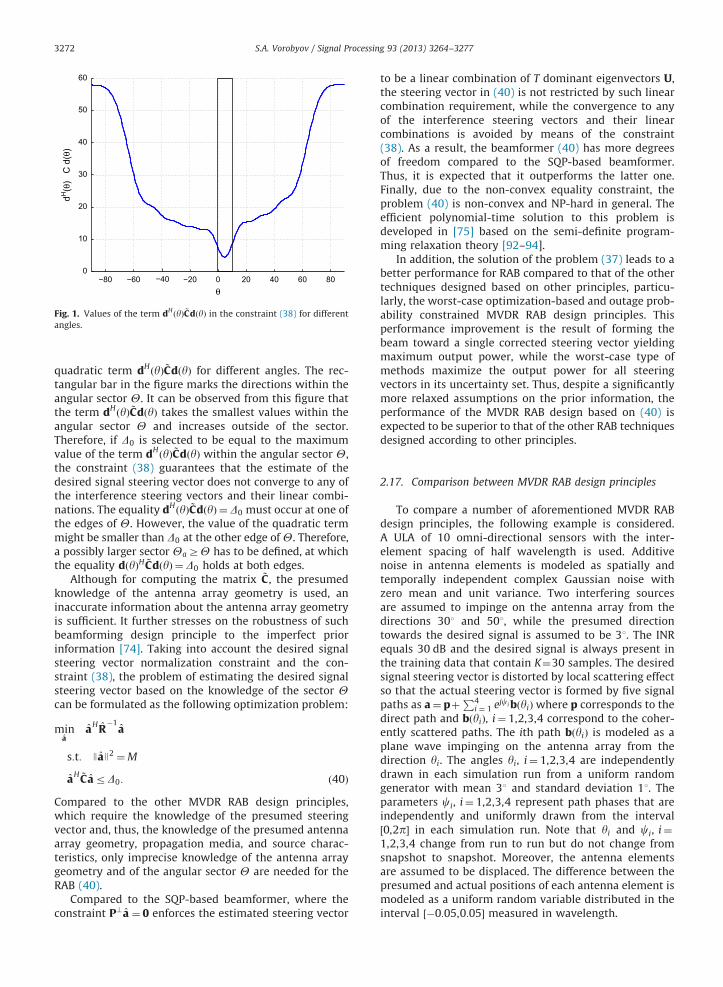
Fig. 1. Values of the term dHðyÞ ~CdðyÞ in the constraint (38) for different

angles.

S.A. Vorobyov / Signal Processing 93 (2013) 3264–32773272

quadratic term dHðyÞ ~CdðyÞ for different angles. The rec-

tangular bar in the figure marks the directions within theangular sector Y. It can be observed from this figure thatthe term dH

ðyÞ ~CdðyÞ takes the smallest values within theangular sector Y and increases outside of the sector.Therefore, if D0 is selected to be equal to the maximumvalue of the term dH

ðyÞ ~CdðyÞ within the angular sector Y,the constraint (38) guarantees that the estimate of thedesired signal steering vector does not converge to any ofthe interference steering vectors and their linear combi-nations. The equality dH

ðyÞ ~CdðyÞ ¼D0 must occur at one ofthe edges of Y. However, the value of the quadratic termmight be smaller than D0 at the other edge of Y. Therefore,a possibly larger sector YaZY has to be defined, at whichthe equality dðyÞH ~CdðyÞ ¼D0 holds at both edges.

Although for computing the matrix ~C, the presumedknowledge of the antenna array geometry is used, aninaccurate information about the antenna array geometryis sufficient. It further stresses on the robustness of suchbeamforming design principle to the imperfect priorinformation [74]. Taking into account the desired signalsteering vector normalization constraint and the con-straint (38), the problem of estimating the desired signalsteering vector based on the knowledge of the sector Ycan be formulated as the following optimization problem:

mina

aH

R�1

a

s:t: JaJ2¼M

aH ~CarD0: ð40Þ

Compared to the other MVDR RAB design principles,which require the knowledge of the presumed steeringvector and, thus, the knowledge of the presumed antennaarray geometry, propagation media, and source charac-teristics, only imprecise knowledge of the antenna arraygeometry and of the angular sector Y are needed for theRAB (40).

Compared to the SQP-based beamformer, where theconstraint P?a ¼ 0 enforces the estimated steering vector

to be a linear combination of T dominant eigenvectors U,the steering vector in (40) is not restricted by such linearcombination requirement, while the convergence to anyof the interference steering vectors and their linearcombinations is avoided by means of the constraint(38). As a result, the beamformer (40) has more degreesof freedom compared to the SQP-based beamformer.Thus, it is expected that it outperforms the latter one.Finally, due to the non-convex equality constraint, theproblem (40) is non-convex and NP-hard in general. Theefficient polynomial-time solution to this problem isdeveloped in [75] based on the semi-definite program-ming relaxation theory [92–94].

In addition, the solution of the problem (37) leads to abetter performance for RAB compared to that of the othertechniques designed based on other principles, particu-larly, the worst-case optimization-based and outage prob-ability constrained MVDR RAB design principles. Thisperformance improvement is the result of forming thebeam toward a single corrected steering vector yieldingmaximum output power, while the worst-case type ofmethods maximize the output power for all steeringvectors in its uncertainty set. Thus, despite a significantlymore relaxed assumptions on the prior information, theperformance of the MVDR RAB design based on (40) isexpected to be superior to that of the other RAB techniquesdesigned according to other principles.

2.17. Comparison between MVDR RAB design principles

To compare a number of aforementioned MVDR RABdesign principles, the following example is considered.A ULA of 10 omni-directional sensors with the inter-element spacing of half wavelength is used. Additivenoise in antenna elements is modeled as spatially andtemporally independent complex Gaussian noise withzero mean and unit variance. Two interfering sourcesare assumed to impinge on the antenna array from thedirections 301 and 501, while the presumed directiontowards the desired signal is assumed to be 31. The INRequals 30 dB and the desired signal is always present inthe training data that contain K¼30 samples. The desiredsignal steering vector is distorted by local scattering effectso that the actual steering vector is formed by five signalpaths as a¼ pþ

P4i ¼ 1 ejci bðyiÞwhere p corresponds to the

direct path and bðyiÞ, i¼ 1,2,3,4 correspond to the coher-ently scattered paths. The ith path bðyiÞ is modeled as aplane wave impinging on the antenna array from thedirection yi. The angles yi, i¼ 1,2,3,4 are independentlydrawn in each simulation run from a uniform randomgenerator with mean 31 and standard deviation 11. Theparameters ci, i¼ 1,2,3,4 represent path phases that areindependently and uniformly drawn from the interval½0,2p� in each simulation run. Note that yi and ci, i¼

1,2,3,4 change from run to run but do not change fromsnapshot to snapshot. Moreover, the antenna elementsare assumed to be displaced. The difference between thepresumed and actual positions of each antenna element ismodeled as a uniform random variable distributed in theinterval ½�0:05,0:05� measured in wavelength.

−20 −15 −10 −5 0 5 10 15 20−20

−15

−10

−5

0

5

10

15

20

25

30

SNR (DB)

OU

TPU

T S

INR

(DB

)

OPTIMAL SINRWORST−CASE−BASED BEAMFORMEREIGENSPACE−BASED BEAMFORMERBEAMFORMER (40)SQP−BASED BEAMFORMERSMI BEAMFORMER

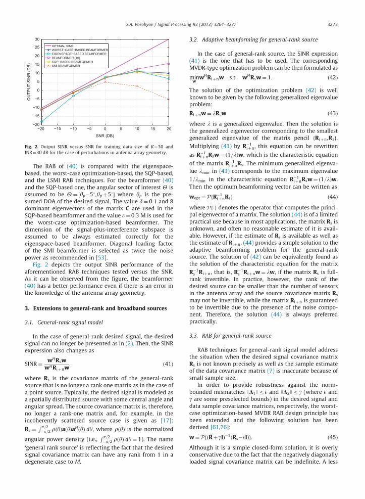
Fig. 2. Output SINR versus SNR for training data size of K¼30 and

INR¼30 dB for the case of perturbations in antenna array geometry.

S.A. Vorobyov / Signal Processing 93 (2013) 3264–3277 3273

The RAB of (40) is compared with the eigenspace-based, the worst-case optimization-based, the SQP-based,and the LSMI RAB techniques. For the beamformer (40)and the SQP-based one, the angular sector of interest Y isassumed to be Y¼ ½yp�51,ypþ51� where yp is the pre-sumed DOA of the desired signal. The value d¼ 0:1 and 8dominant eigenvectors of the matrix C are used in theSQP-based beamformer and the value e¼ 0:3 M is used forthe worst-case optimization-based beamformer. Thedimension of the signal-plus-interference subspace isassumed to be always estimated correctly for theeigenspace-based beamformer. Diagonal loading factorof the SMI beamformer is selected as twice the noisepower as recommended in [53].

Fig. 2 depicts the output SINR performance of theaforementioned RAB techniques tested versus the SNR.As it can be observed from the figure, the beamformer(40) has a better performance even if there is an error inthe knowledge of the antenna array geometry.

3. Extensions to general-rank and broadband sources

3.1. General-rank signal model

In the case of general-rank desired signal, the desiredsignal can no longer be presented as in (2). Then, the SINRexpression also changes as

SINR¼wHRsw

wHRiþnwð41Þ

where Rs is the covariance matrix of the general-ranksource that is no longer a rank one matrix as in the case ofa point source. Typically, the desired signal is modeled asa spatially distributed source with some central angle andangular spread. The source covariance matrix is, therefore,no longer a rank-one matrix and, for example, in theincoherently scattered source case is given as [17]:

Rs ¼R p=2�p=2 rðyÞaðyÞa

HðyÞ dy, where rðyÞ is the normalized

angular power density (i.e.,R p=2�p=2 rðyÞ dy¼ 1). The name

‘general rank source’ is reflecting the fact that the desiredsignal covariance matrix can have any rank from 1 in adegenerate case to M.

3.2. Adaptive beamforming for general-rank source

In the case of general-rank source, the SINR expression(41) is the one that has to be used. The correspondingMVDR-type optimization problem can be then formulated as

minw

wHRiþnw s:t: wHRsw¼ 1: ð42Þ

The solution of the optimization problem (42) is wellknown to be given by the following generalized eigenvalueproblem:

Riþnw¼ lRsw ð43Þ

where l is a generalized eigenvalue. Then the solution isthe generalized eigenvector corresponding to the smallestgeneralized eigenvalue of the matrix pencil fRiþn,Rsg.

Multiplying (43) by R�1iþn, this equation can be rewritten

as R�1iþnRsw¼ ð1=lÞw, which is the characteristic equation

of the matrix R�1iþnRs. The minimum generalized eigenva-

lue lmin in (43) corresponds to the maximum eigenvalue

1=lmin in the characteristic equation R�1iþnRsw¼ ð1=lÞw.

Then the optimum beamforming vector can be written as

wopt ¼PfR�1iþnRsg ð44Þ

where Pf�g denotes the operator that computes the princi-pal eigenvector of a matrix. The solution (44) is of a limitedpractical use because in most applications, the matrix Rs isunknown, and often no reasonable estimate of it is avail-able. However, if the estimate of Rs is available as well asthe estimate of Riþn, (44) provides a simple solution to theadaptive beamforming problem for the general-ranksource. The solution of (42) can be equivalently found asthe solution of the characteristic equation for the matrix

R�1s Riþn, that is, R�1

s Riþnw¼ lw, if the matrix Rs is full-

rank invertible. In practice, however, the rank of thedesired source can be smaller than the number of sensorsin the antenna array and the source covariance matrix Rs

may not be invertible, while the matrix Riþn is guaranteedto be invertible due to the presence of the noise compo-nent. Therefore, the solution (44) is always preferredpractically.

3.3. RAB for general-rank source

RAB techniques for general-rank signal model addressthe situation when the desired signal covariance matrixRs is not known precisely as well as the sample estimateof the data covariance matrix (7) is inaccurate because ofsmall sample size.

In order to provide robustness against the norm-bounded mismatches JD1JrE and JD2Jrg (where E andg are some preselected bounds) in the desired signal anddata sample covariance matrices, respectively, the worst-case optimization-based MVDR RAB design principle hasbeen extended and the following solution has beenderived [61,76]:

w¼PfðRþgIÞ�1ðRs�EIÞg: ð45Þ

Although it is a simple closed-form solution, it is overlyconservative due to the fact that the negatively diagonallyloaded signal covariance matrix can be indefinite. A less

τ τ

τ

τ

τ

τ

w11 w12 w1P

w21 w22 w2P

wN1 wN2 wNP

Δ1

Δ2

ΔN

Σ

Fig. 3. Block scheme of the presteered broadband adaptive beamformer.

S.A. Vorobyov / Signal Processing 93 (2013) 3264–32773274

conservative RAB problem formulation, which enforcesthe matrix RsþD1 to be positive semi-definite has beenconsidered in [77]. Defining Rs ¼Q HQ , which is, forexample, the Cholesky decomposition, the correspondingRAB problem for a norm bounded-mismatch JDJrZ(where Z is some bound value found based on the boundvalue E) to the matrix Q is given as [77]

minw

maxJD2Jrg

wHðRþD2Þw

s:t: minJDJrZ

wHðQþDÞHðQþDÞwZ1: ð46Þ

If the mismatch of the signal covariance matrix is smallenough, the optimization problem (46) can be equiva-lently recast as

minw

wHðRþgIÞw

s:t: JQwJ�ZJwJZ1: ð47Þ

Due to the non-convex (difference-of-convex functions)constraint, the problem (47) is non-convex. Although thedifference-of-convex functions (DC) programming pro-blems are believed to be NP-hard in general, the problem(47) is shown to have very efficient polynomial-timesolution [78,79] by applying the polynomial-time DC(POTDC) method [95].

3.4. Broadband signal model

In the broadband case, the desired signal and/or theinterference signals is widely spread in the frequencydomain. As a result, it is not possible to factorize theprocessing in temporal and spatial parts. Therefore, jointspace-time adaptive processing (STAP) has to be performed.

Let the number of taps in the time domain be denotedas P. Let also the M array sensors be uniformly spaced

with the inter-element spacing less than or equal to c=2f u,

where f u ¼ f cþBs=2 is the maximum frequency of thedesired signal/maximum passband frequency, fc is thecarrier frequency, Bs is the signal bandwidth, and c is thewave propagation speed. The received signal at the ithsensor goes to a broadband presteering delay filter withthe delay Di. Let the output of the broadband presteeringdelay filter be sampled with the sampling frequency

f s ¼ 1=t where t is the sampling time and fs is greaterthan or equal to 2fu. Then the MP�1 stacked snapshotvector containing P delayed presteered data vectors is thedata vector x (k). The beamformer output y (k) is then

given as: yðkÞ ¼wT xðkÞ where w is the real-valued MP�1beamformer weight vector, i.e., wMðp�1Þþm ¼wm,p. The

above described modeling is shown schematically inFig. 3.

In the broadband case, the steering vector also

depends on frequency and is given as aðf ,yÞ ¼½ej2pfz1sinðyÞ=c , . . . ,ej2pfzM sinðyÞ=c�T where zi is the ith sensorlocation. The overall MP�1 steering vector can be

expressed as aðf ,yÞ ¼ dðf Þ � ðBðf Þaðf ,yÞÞ, where dðf Þ9½1,

e�j2pft, . . . ,e�j2pf ðP�1Þt�T , Bðf Þ9diagfe�j2pfD1 , . . . ,e�j2pfDM g,and � denotes the Kronecker product. Then the arrayresponse to a plane wave with the frequency f and angle

of arrival y is Hðf ,yÞ ¼wT aðf ,yÞ.

The presteering delays are selected so that the desiredsignal arriving from the look direction y0 appears coher-ently at the output of the M presteering filters so that [3]

Bðf Þaðf ,y0Þ ¼ 1M ð48Þ

where 1M is the M�1 vector containing all ones. Then thesteering vector towards the look direction y0 becomes

aðf ,y0Þ ¼ dðf Þ � 1M ð49Þ

and the array response towards such signal becomes

Hðf ,y0Þ ¼wT aðf ,y0Þ ¼wT C0dðf Þ ð50Þ

where C09IP � 1M .

3.5. Broadband beamforming

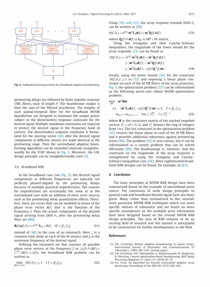
One popular approach to broadband beamforming is todecompose the baseband waveforms into narrowbandfrequency components by means of fast Fourier transform(FFT) [81,96]. Subsequently, the subbands can be pro-cessed independently from each other using narrowbandbeamforming techniques as it is shown in Fig. 4. Then anyof the above discussed adaptive beamforming methodscan be used to solve each narrowband beamformingproblem. Thus, P adaptive beamforming problems, eachfor the beamforming vector of length M, are needed to besolved. The time-domain beamformer output samples areobtained by applying an inverse FFT (IFFT) of the outputsamples of the individual narrowband beamformers.However, such FFT-based broadband beamforming tech-nique is non-optimum, since correlations between thefrequency domain snapshot vectors of different subbandsare not taken into account. Although these correlationscan be reduced by increasing the FFT length, the latterrequires a larger training data set [96].

Based on the broadband data and beamforming mod-els, another approach to broadband beamforming thatdoes not require subband decomposition exists [3]. Theblock scheme of such adaptive beamformer is shown inFig. 3. This beamformer uses a presteering delay front-endconsisting of presteering delay filters to time-align thedesired signal components in different sensors. Then the

FFT FFT FFT

narrowbandadaptive

beamformer

narrowbandadaptive

beamformer

narrowbandadaptive

beamformer

Σ

(subband P)(subband 2)(subband 1)

Fig. 4. Subband processing scheme for broadband adaptive beamforming.

S.A. Vorobyov / Signal Processing 93 (2013) 3264–3277 3275

presteering delays are followed by finite impulse response(FIR) filters, each of length P. The beamformer output isthen the sum of the filtered waveforms. The weights ofsuch spatial-temporal filter for the broadband MVDRbeamformer are designed to minimize the output powersubject to the distortionless response constraint for thedesired signal. Multiple mainbeam constraints are requiredto protect the desired signal in the frequency band ofinterest. The distortionless response constraint is formu-lated for the steering vector (49) after the desired signalcomponents in different sensors are made identical at thepresteering stage. Then the narrowband adaptive beam-forming algorithms can be extended relatively straightfor-wardly for the STAP shown in Fig. 3. Moreover, the GSCdesign principle can be straightforwardly used [3].

3.6. Broadband RAB

In the broadband case (see Fig. 3), the desired signalcomponents at different frequencies are typically notperfectly phased-aligned by the presteering delaysbecause of multiple practical imperfections. The reasonsfor imperfections are accentually the same as in thenarrowband case with an addition of more error sourcessuch as the presteering delay quantization effects. There-fore, there are errors that can be modeled in terms of thephase error vector dðf Þ that is the function of thefrequency f. Then the actual components of the desiredsignal arriving from DOA ys after the presteering delayfilter are [80]

Bðf Þaðf ,ysÞ ¼ ejpfB1Mþdðf Þ 8f 2 ½f l, f u� ð51Þ

instead of (48) in the case of no mismatch. Here B is acommon time delay at each of the M sensors and fl is theminimum frequency of the desired signal.

Defining the mismatch set that contains all possiblephase error vectors at the frequency f as Aeðf Þ9fdðf Þ 2CM9Jdðf ÞJreðf Þg, the broadband RAB problem can bewritten as

mindðf Þ2Aeðf Þ

9Hðf ,ysÞ9Z1 8 f 2 ½f l,f u�: ð52Þ

Using (50) and (51), the array response towards DOA ys

can be written as [80]

Hðf ,ysÞ ¼ ejpfBwT C0dðf ÞþwT Q ðf Þdðf Þ ð53Þ

where Q ðf Þ9dðf Þ � IM is MP�M matrix.Using the triangular and then Cauchy–Schwarz

inequalities, the magnitude of the lower bound for thearray responde (53) can be found as

9Hðf ,ysÞ9¼ 9ejpfBwT C0dðf ÞþwT Q ðf Þdðf Þ9

Z9wT C0dðf Þ9�9wT Q ðf Þdðf Þ9

Z9wT C0dðf Þ9�eðf ÞJQ Tðf ÞwJ: ð54Þ

Finally, using the lower bound (54) for the constraint9Hðf ,ysÞ9Z1 in (52) and imposing a linear phase con-straint on each of the M FIR filters of the array processor,Fig. 3, the optimization problem (52) can be reformulatedas the following worst-case robust MVDR optimizationproblem:

minw

wT Rw

s:t: 9wT C0dðf Þ9�eðf ÞJQ Tðf ÞwJZ1, f 2 ½f l, f u�

wm,l ¼wm,P�lþ1 8m 2 ZM1 , l 2 ZPc�1

1 ð55Þ

where R is the covariance matrix of the stacked snapshotvectors, Pc ¼ ðPþ1Þ=2, and Zj

i denotes the ring of integersfrom i to j. The last constraint in the optimization problem(55) ensures the linear phase at each of the M FIR filtersand it provides additional robustness against presteeringerrors [80]. The problem (55) is non-convex, but it can bereformulated as a convex problem that can be solvedefficiently [80]. The disadvantage is, however, that theconstraint on the magnitude of the array response isstrengthened by using the triangular and Cauchy–Schwarz inequalities (see (54)). More sophisticated broad-band RAB designs can be found, for example, in [83].

4. Conclusion

The basic principles of MVDR RAB design have beensummarized based on the example of narrowband pointsource. The extensions of some design principles togeneral-rank and broadband desired signal have also beengiven. Many (other than summarized in this tutorial)more particular MVDR RAB techniques which use morespecific notions of robustness and are based on morespecific assumptions on the available prior informationhave been designed based on the revised MVDR RABdesign principles. The area of RAB remains to be anexciting field of research and this tutorial is anticipatedto be constructive for further developments in the field.

References

[1] A.B. Gershman, Robust adaptive beamforming in sensor arrays,International Journal of Electronics and Communications 53(December) (1999) 305–314. (invited paper).

[2] A.B. Gershman, N.D. Sidiropoulos, S. Shahbazpanahi, M. Bengtsson,B. Ottersten, Convex optimization-based beamforming, IEEE SignalProcessing Magazine 27 (June (3)) (2010) 62–75.

[3] O.L. Frost, An algorithm for linearly constrained adaptive arrayprocessing, Proceedings of the IEEE 60 (1972) 926–935.

S.A. Vorobyov / Signal Processing 93 (2013) 3264–32773276

[4] N.K. Jablon, Adaptive beamforming with the generalized sidelobecanceller in the presence of array imperfections, IEEE Transactionson Antennas and Propagation 34 (1986) 996–1012.

[5] J.C. Preisig, Robust maximum energy adaptive matched field proces-sing, IEEE Transactions on Signal Processing 42 (1994) 1585–1593.

[6] D.D. Feldman, L.J. Griffiths, A projection approach to robust adap-tive beamforming, IEEE Transactions on Signal Processing 42 (April)(1994) 867–876.

[7] J.L. Yu, C.C. Yeh, Generalized eigenspace-based beamformers, IEEETransactions on Signal Processing 43 (1995) 2453–2461.

[8] U. Nickel, On the application of subspace methods for small samplesize, International Journal of Electronics and Communications 51(1997) 279–289.

[9] E.K. Hung, R.M. Turner, A fast beamforming algorithm for largearrays, IEEE Transactions on Aerospace and Electronic Systems 19(July) (1983) 598–607.

[10] A.B. Gershman, G.V. Serebryakov, J.F. Boehme, Constrained Hung-Turner adaptive beamforming algorithm with additional robust-ness to wideband and moving jammers, IEEE Transactions onAntennas and Propagation 44 (1996) 361–367.

[11] C.H. Gierull, Performance analysis of fast projections of the Hung-Turner type for adaptive beamforming, Signal Processing 50 (1996)17–28.

[12] T.J. Shan, T. Kailath, Adaptive beamforming for coherent signals andinterference, IEEE Transactions on Acoustics, Speech, and SignalProcessing 33 (1985) 527–536.

[13] M.D. Zoltowski, On the performance of the MVDR beamformer inthe presence of correlated interference, IEEE Transactions onAcoustics, Speech, and Signal Processing 36 (1988) 945–947.

[14] A.B. Gershman, V.T. Ermolaev, Optimal subarray size for spatialsmoothing, IEEE Signal Processing Letters 2 (1995) 28–30.

[15] R.T. Williams, S. Prasad, A.K. Mahalanabis, L. Sibul, An improvedspatial smoothing technique for bearing estimation in a multipathenvironment, IEEE Transactions on Acoustics, Speech, and SignalProcessing 36 (1988) 425–432.

[16] K. Takao, N. Kikuma, T. Yano, Toeplization of correlation matrix inmultipath environment, in: Proceedings of the ICASSP’86, Tokyo,Japan, 1986, pp. 1873–1876.

[17] A.B. Gershman, C.F. Mecklenbraeucker, J.F. Boehme, Matrix fittingapproach to direction of arrival estimation with imperfect spatialcoherence of wavefronts, IEEE Transactions on Signal Processing45(1997) 1894–1899.

[18] A.B. Gershman, V.I. Turchin, V.A. Zverev, Experimental results oflocalization of moving underwater signal by adaptive beamforming,IEEE Transactions on Signal Processing 43 (October) (1995) 2249–2257.

[19] Y.J. Hong, C.C. Yeh, D.R. Ucci, The effect of a finite-distance signalsource on a far-field steering Applebaum array – two dimensionalarray case, IEEE Transactions on Antennas and Propagation 36(April) (1988) 468–475.

[20] J. Goldberg, H. Messer, Inherent limitations in the localization of acoherently scattered source, IEEE Transactions on Signal Processing46 (December) (1998) 3441–3444.

[21] O. Besson, P. Stoica, Decoupled estimation of DOA and angularspread for a spatially distributed source, IEEE Transactions onSignal Processing 48 (July) (2000) 1872–1882.

[22] D. Astely, B. Ottersten, The effects of local scattering on direction ofarrival estimation with MUSIC, IEEE Transactions on Signal Proces-sing 47 (December) (1999) 3220–3234.

[23] R.J. Mallioux, Covariance matrix augmentation to produce adaptivearray pattern troughs, Electronic Letters 31 (1995) 771–772.

[24] A.B. Gershman, U. Nickel, J.F. Boehme, Adaptive beamformingalgorithms with robustness against jammer motion, IEEE Transac-tions on Signal Processing 45 (1997) 1878–1885.

[25] J.R. Guerci, Theory and application of covariance matrix tapers torobust adaptive beamforming, IEEE Transactions on Signal Proces-sing 47 (April) (2000) 977–985.

[26] M.A. Zatman, Comment on theory and application of covariancematrix tapers for robust adaptive beamforming, IEEE Transactionson Signal Processing 48 (June) (2000) 1796–1800.

[27] S.D. Hayward, Adaptive beamforming for rapidly moving arrays, in:Proceedings of the International Conference on Radar, Bejing,China, 1996, pp. 546–549.

[28] K. Takao, K. Komiyama, An adaptive antenna for rejection ofwideband interference, IEEE Transactions on Aerospace and Elec-tronic Systems 16 (1980) 452–459.

[29] M. Bengtsson, B. Ottersten, Optimal and suboptimal transmitbeamforming, in: L. Godara (Ed.), Handbook of Antennas inWireless Communications, CRC Press, Boca Raton, FL, 2001.(Chapter 18).

[30] S. Verdu, Multiuser Detection, Cambridge University Press,Cambridge, UK, 1998.

[31] K. Zarifi, S. Shahbazpanahi, A.B. Gershman, Z.-Q. Luo, Robust blindmultiuser detection based on the worst-case performance optimi-zation of the MMSE receiver, IEEE Transactions on Signal Processing53 (January) (2005) 295–305.

[32] S.A. Vorobyov, Robust CDMA multiuser detectors: probability-constrained versus the worst-case based design, IEEE SignalProcessing Letters 15 (2008) 273–276.

[33] S. Shahbazpanahi, M. Beheshti, A.B. Gershman, M. Gharavi-Alkhansari, K.M. Wong, Minimum variance linear receivers formulti-access MIMO wireless systems with space-time block coding,IEEE Transactions on Signal Processing 52 (December) (2004)3306–3313.

[34] Y. Rong, S.A. Vorobyov, A.B. Gershman, Robust linear receivers formulti-access space-time block coded MIMO systems: A probabil-istically constrained approach, IEEE Journal of Selected Areas inCommunications 24 (August) (2006) 1560–1570.

[35] N.D. Sidiropoulos, T.N. Davidson, Z.-Q. Luo, Transmit beamformingfor physical-layer multicasting, IEEE Transactions on Signal Proces-sing 54 (June) (2006) 2239–2251.

[36] E. Karipidis, N.D. Sidiropoulos, Z.-Q. Luo, Far-field multicast beam-forming for uniform linear antenna arrays, IEEE Transactions onSignal Processing 55 (October) (2007) 4916–4927.

[37] K.T. Phan, S.A. Vorobyov, N.D. Sidiropoulos, C. Tellambura, Spec-trum sharing in wireless networks via QoS-aware secondary multi-cast beamforming, IEEE Transactions on Signal Processing 57 (June)(2009) 2323–2335.

[38] V. Havary-Nassab, S. Shahbazpanahi, A. Grami, Z.-Q. Luo, Distributedbeamforming for relay networks based on second-order statistics ofthe channel state information, IEEE Transactions on Signal Processing56 (September) (2008) 4306–4316.

[39] B. Widrow, P.E. Mantey, J.L. Griffiths, B.B. Goode, Adaptive antennasystems, Proceeding of the IEEE 55 (December) (1967) 2143–2159.

[40] R.A. Monzingo, T.W. Miller, Introduction to Adaptive Arrays, Wiley,NY, 1980.

[41] B. Widrow, S.D. Stearns, Adaptive Signal Processing, Prentice Hall,Englewood Cliffs, NJ, 1985.

[42] H.L. Van Trees, Optimum Array Processing, Wiley, NY, 2002.[43] S. Haykin, J. Litva, T. Shepherd (Eds.), Radar Array Processing,

Springer-Verlag, 1992.[44] A. Farina, Antenna-Based Signal Processing Techniques for Radar

Systems, Artech House, Norwood, MA, 1992.[45] R.J. Vaccaro (Ed.), The past, present, and the future of underwater

acoustic signal processing, IEEE Signal Processing Magazine15 (July) (1998) 21–51.

[46] T.S. Rapapport (Ed.), Smart Antennas: Adaptive Arrays, Algorithms,and Wireless Position Location, IEEE Press, 1998.

[47] A.B. Gershman, N.D. Sidiropoulos (Eds.), Space-Time Processing forMIMO Communications, John Wiley and Sons, 2005.

[48] Y. Kameda, J. Ohga, Adaptive microphone-array system for noisereduction, IEEE Transactions on Acoustics, Speech, and SignalProcessing 34 (December) (1986) 1391–1400.

[49] S.W. Ellingson, G.A. Hampson, A subspace-tracking approach tointerference nulling for phased array-based radio telescopes, IEEETransactions on Antennas and Propagation 50 (January) (2002)25–30.

[50] A. Leshem, J. Christou, B.D. Jeffs, E. Kuruoglu, A.J. van der Veen (Eds.),Issue on signal processing for space research and astronomy, IEEEJournal of Selected Topics in Signal Processing 2(5, October) (2008).

[51] K. Sekihara, Performance of an MEG adaptive beamformer sourcereconstruction technique in the presence of adaptive low-rank interference, IEEE Transactions on Biomedical Engineering51 (January) (2004) 90–99.

[52] K.-M. Chen, D. Misra, H. Wang, H.-R. Chuang, E. Postow, An X-bandmicrowave life-detection system, IEEE Transactions on BiomedicalEngineering 33 (July) (1986) 697–701.

[53] H. Cox, R.M. Zeskind, M.H. Owen, Robust adaptive beamforming,IEEE Transactions on Acoustic, Speech, and Signal Processing35 (October) (1987) 1365–1376.

[54] Y.I. Abramovich, Controlled method for adaptive optimization offilters using the criterion of maximum SNR, Radio Engineering andElectronic Physics 26 (March) (1981) 87–95.

[55] B.D. Carlson, Covariance matrix estimation errors and diagonalloading in adaptive arrays, IEEE Transactions on Aerospace andElectronic Systems 24 (July (7)) (1988) 397–401.

[56] B. Widrow, K.M. Duvall, R.P. Gooch, W.C. Newman, Signal cancella-tion phenomena in adaptive antennas: causes and cures, IEEETransactions on Antennas and Propagation 30 (1982) 469–478.

S.A. Vorobyov / Signal Processing 93 (2013) 3264–3277 3277

[57] J.W. Kim, C.K. Un, An adaptive array robust to beam pointing error,IEEE Transactions on Signal Processing 40 (June) (1992) 1582–1584.

[58] L. Chang, C.C. Yeh, Performance of DMI and eigenspace-basedbeamformers, IEEE Transactions on Antennas and Propagation 40(November) (1992) 1336–1347.

[59] S.A. Vorobyov, A.B. Gershman, Z.-Q. Luo, Robust adaptive beam-forming using worst-case performance optimization: a solution tothe signal mismatch problem, IEEE Transactions on Signal Proces-sing 51 (February) (2003) 313–324.

[60] R.G. Lorenz, S.P. Boyd, Robust minimum variance beamforming, IEEETransactions on Signal Processing 53 (May) (2005) 1684–1696.

[61] A.B. Gershman, Z.-Q. Luo, S. Shahbazpanahi, Robust adaptivebeamforming based on worst-case performance optimizationin: P. Stoica, J. Li (Eds.), Robust Adaptive Beamforming, Wiley,Hoboken, NJ, 2006, pp. 49–89.

[62] G.A. Fabrizio, A.B. Gershman, M.D. Turley, Robust adaptive beam-forming for HF surface wave over-the-horizon radar, IEEE Transac-tions on Aerospace and Electronic Systems 40 (April) (2004)510–625.

[63] J. Li, P. Stoica, Z. Wang, On robust Capon beamforming and diagonalloading, IEEE Transactions on Signal Processing 51 (July) (2003)1702–1715.

[64] S.A. Vorobyov, A.B. Gershman, Z.-Q. Luo, N. Ma, Adaptive beam-forming with joint robustness against mismatched signal steeringvector and interference nonstationarity, IEEE Signal ProcessingLetters 11 (February) (2004) 108–111.

[65] J. Li, P. Stoica (Eds.), Robust Adaptive Beamforming, John Wiley andSons, New York, NY, 2005.

[66] P. Stoica, Z. Wang, J. Li, Robust Capon beamforming, IEEE SignalProcessing Letters 10 (June (6)) (2003) 172–175.

[67] J. Li, P. Stoica, Z. Wang, Doubly constrained robust capon beamfor-mer, IEEE Transactions on Signal Processing 52 (September) (2004)2407–2423.

[68] S.A. Vorobyov, H. Chen, A.B. Gershman, On the relationshipbetween robust minimum variance beamformers with probabilisticand worst-case distrortionless response constraints, IEEE Trans-actions on Signal Processing 56 (November) (2008) 5719–5724.

[69] S.A. Vorobyov, A.B. Gershman, Y. Rong, On the relationship betweenthe worst-case optimization-based and probability-constrainedapproaches to robust adaptive beamforming, in: Proceedings ofthe 32nd IEEE International Conference on Acoustics, Speech, andSignal Processing, Honolulu, Hawaii, USA, April 2007, pp. 977–980.

[70] M. Ruebsamen, A.B. Gershman, Robust adaptive beamformingusing multi-dimensional covariance fitting, IEEE Transactions onSignal Processing 60 (February) (2012) 740–753.

[71] A. Pezeshki, B.D. Van Veen, L.L. Scharf, H. Cox, M. Lundberg,Eigenvalue beamforming using a multi-rank MVDR beamformerand subspace selection, IEEE Transactions on Signal Processing 56(May) (2008) 1954–1967.

[72] A. Hassanien, S.A. Vorobyov, K.M. Wong, Robust adaptive beam-forming using sequential programming: an iterative solution to themismatch problem, IEEE Signal Processing Letters 15 (2008)733–736.

[73] L. Lei, J.P. Lie, A.B. Gershman, C.M.S. See, Robust adaptive beam-forming in partly calibrated sparse sensor arrays, IEEE Transactionson Signal Processing 58 (March) (2010) 1661–1667.

[74] A. Khabbazibasmenj, S.A. Vorobyov, A. Hassanien, Robust adaptivebeamforming via estimating steering vector based on semidefiniterelaxation, in: Proceedings of the 44th Asilomar Conference onSignals, Systems and Computers, Pacific Grove, California, Novem-ber 2010, pp. 1102–1106.

[75] A. Khabbazibasmenj, S.A. Vorobyov, A. Hassanien, Robust adaptivebeamforming based on steering vector estimation with as little aspossible prior information, IEEE Transactions on Signal Processing60 (June) (2012) 2974–2987.

[76] S. Shahbazpanahi, A.B. Gershman, Z.-Q. Luo, K.M. Wong, Robustadaptive beamforming for general-rank signal models, IEEE Trans-actions on Signal Processing 51 (September) (2003) 2257–2269.

[77] H.H. Chen, A.B. Gershman, Robust adaptive beamforming forgeneral-rank signal models with positive semi-definite constraints,

in: Proceedings of the IEEE International Conference on Acoustic,Speech, and Signal Processing, Las Vegas, USA, April 2008,pp. 2341–2344.

[78] A. Khabbazibasmenj, S.A. Vorobyov, A computationally efficientrobust adaptive beamforming for general-rank signal model withpositive semi-definite constraint, in: Proceedings of the IEEE Inter-national Workshop on Computational Advances in Multi-SensorAdaptive Processing, San Juan, Puerto Rico, December 2011,pp. 185–188.

[79] A. Khabbazibasmenj, S.A. Vorobyov, Robust adaptive beamformingfor general-rank signal model with positive semi-definite con-straint via POTDC, IEEE Transactions on Signal Processing, sub-mitted for publication /http://www.ece.ualberta.ca/�vorobyov/TPS13a.pdfS.

[80] A. El-Keyi, T. Kirubarajan, A.B. Gershman, Adaptive widebandbeamforming with robustness against presteering errors, in: Pro-ceedings of the IEEE Workshop on Sensor Arrays and Multi-ChannelProcessing, Waltham, MA, USA, July 2006, pp. 11–15.

[81] Z. Wang, J. Li, P. Stoica, T. Nishida, M. Sheplak, Constant beamwidthand constant-powerwidth wideband robust Capon beamformersfor acoustic imaging, Journal of the Acoustical Society of America116 (3) (2004) 1621–1631.

[82] M. Ruebsamen, Advanced Direction-of-Arrival Estimation andBeamforming Techniques for Multiple Antenna Systems, Ph.D.Thesis, Darmstadt University of Technology, 2011 (Chapter 5).

[83] M. Ruebsamen, A. El-Keyi, A.B. Gershman, T. Kirubarajan, Robustbroadband adaptive beamforming using convex optimization, in:D.P. Palomar, Y.C. Eldar (Eds.), Convex Optimization in SignalProcessing and Communications, Cambridge University Press,2010, pp. 315–339. (Chapter 9).

[84] O. Leodit, M. Wolf, Improved estimation of the covariance matrix ofthe stock returns with an application to portfolio selection, Journalof Empirical Finance 10 (2003) 603–621.

[85] Y. Gu, A. Leshem, Robust adaptive beam forming based on inter-ference covariance matrix reconstruction and steering vectorestimation, IEEE Transactions on Signal Processing 60 (July) (2012)3881–3885.

[86] I.S. Reed, J.D. Mallett, L.E. Brennan, Rapid convergence rate inadaptive arrays, IEEE Transactions on Aerospace and ElectronicSystems 10 (November) (1974) 853–863.

[87] L.C. Godara, The effect of phase-shift errors on the performance ofan antenna-array beamformer, IEEE Journal of Oceanic Engineering10 (July) (1985) 278–284.

[88] Special issue on adaptive antennas, IEEE Transactions on Antennasand Propagation, 24 (1976).

[89] A.N. Tikhonov, V.Y. Arsenin, Solution to Ill-Posed Problems,V.H. Winston, Washington, DC, 1977.

[90] J.K. Thomas, L.L. Scharf, D.W. Tufts, The probability of a subspaceswap in the SVD, IEEE Transactions on Signal Processing 43 (March)(1995) 730–736.

[91] Z.-Q. Luo, W. Yu, An introduction to convex optimization forcommunications and signal processing, IEEE Journal of SelectedAreas in Communications 24 (August) (2006) 20–34.

[92] Z.-Q. Luo, W.-K. Ma, A.M.-C. So, Y. Ye, S. Zhang, Semidefiniterelaxation of quadratic optimization problems, IEEE Signal Proces-sing Magazine 27 (May (3)) (2010) 20–34.

[93] Y.S. Nesterov, Semidefinite relaxation and nonconvex quadraticoptimization, Optimization Methods and Software 9 (1–3) (1998)141–160.

[94] S. Zhang, Quadratic maximization and semidefinite relaxation,Mathematics Programs A 87 (2000) 453–465.

[95] A. Khabbazibasmenj, F. Roemer, S.A. Vorobyov, M. Haardt, Sum-ratemaximization in two-way AF MIMO relaying: polynomial timesolutions to a class of DC programming problems, IEEE Trans-actions on Signal Processing 60 (October (10)) (2012) 5478–5493.

[96] T.J. Cornwell, A novel principle for optimization of the instanta-neous Fourier plane coverage of correlation arrays, IEEE Transac-tions on Antennas and Propagation 36 (8) (1988) 1165–1167.