Principy nanomechanické analýzy heterogenních materiálů

1/301/36

Principy nanomechanické analýzy heterogenních materiálů. Dekonvoluce a

homogenizace.

Doc. Ing. Jiří Němeček, Ph.D., DSc.

ČVUT Praha, Fakulta stavební

Tvorba výukových materiálů byla podpořena projektem OPVVV, Rozvoj výzkumně orientovaného studijního programu Fyzikální a materiálové inženýrství, CZ.02.2.69/0.0/0.0/16_018/0002274 (2017-18)

D32MPO - Mikromechanika a popis mikrostruktury materiálů – přednáška 04

2/302/36

Outline

Introduction and motivation

Principles of nanomechanical analysis on heterogeneous

materials. Nanoindentation, SEM, image analysis.

Nanomechanical analysis of distinct material phases applied to

cement paste, Alkali-activated Fly ash, Gypsum

Up-scaling phase properties to upper composite level

3/303/36

Introduction

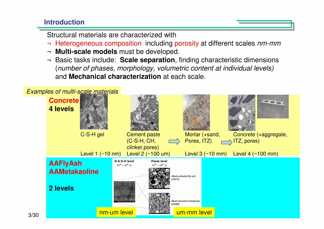
Structural materials are characterized with

¬ Heterogeneous composition including porosity at different scales nm-mm

¬ Multi-scale models must be developed.¬ Basic tasks include: Scale separation, finding characteristic dimensions

(number of phases, morphology, volumetric content at individual levels)

and Mechanical characterization at each scale.

Examples of multi-scale materials

Concrete4 levels

C-S-H gel

Level 1 (~10 nm)

Cement paste(C-S-H, CH, clinker,pores)Level 2 (~100 um)

Mortar (+sand, Pores, ITZ)

Level 3 (~10 mm)

Concrete (+aggregate,ITZ, pores)

Level 4 (~100 mm)

AAFlyAshAAMetakaoline

2 levels

nm-um level um-mm level

4/304/36

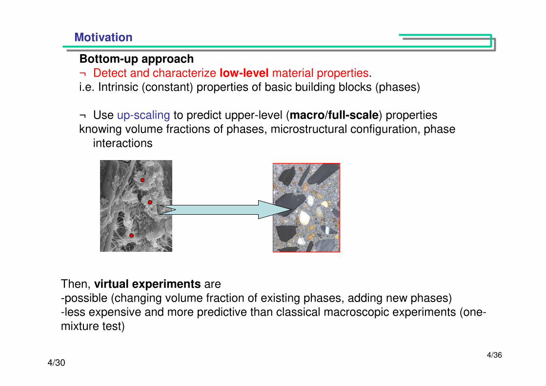
Motivation

Bottom-up approach¬ Detect and characterize low-level material properties.i.e. Intrinsic (constant) properties of basic building blocks (phases)

¬ Use up-scaling to predict upper-level (macro/full-scale) propertiesknowing volume fractions of phases, microstructural configuration, phase

interactions

Then, virtual experiments are -possible (changing volume fraction of existing phases, adding new phases)-less expensive and more predictive than classical macroscopic experiments (one-

mixture test)

5/305/36

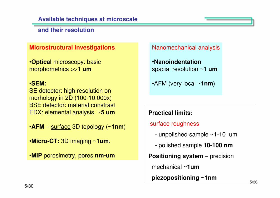
Available techniques at microscale

and their resolution

Practical limits:

surface roughness

- unpolished sample ~1-10 um

- polished sample 10-100 nm

Positioning system – precision

mechanical ~1um

piezopositioning ~1nm

Microstructural investigations

•Optical microscopy: basic morphometrics >>1 um

•SEM:SE detector: high resolution on morhology in 2D (100-10.000x)BSE detector: material constrast

EDX: elemental analysis ~5 um

•AFM – surface 3D topology (~1nm)

•Micro-CT: 3D imaging ~1um.

•MIP porosimetry, pores nm-um

Nanomechanical analysis

•Nanoindentationspacial resolution ~1 um

•AFM (very local ~1nm)

6/306/36

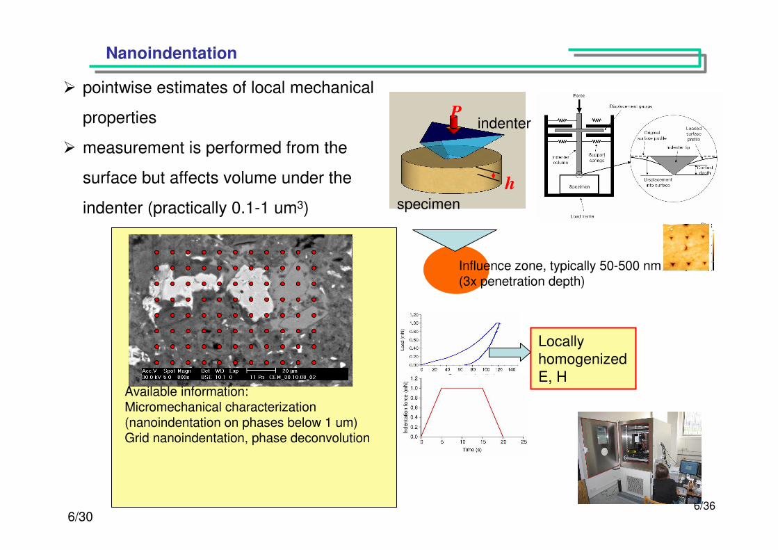
Available information:Micromechanical characterization (nanoindentation on phases below 1 um) Grid nanoindentation, phase deconvolution

pointwise estimates of local mechanical

properties

measurement is performed from the

surface but affects volume under the

indenter (practically 0.1-1 um3)

Nanoindentation

P

h

specimen

indenter

Influence zone, typically 50-500 nm(3x penetration depth)

Locally

homogenized

E, H

7/307/36

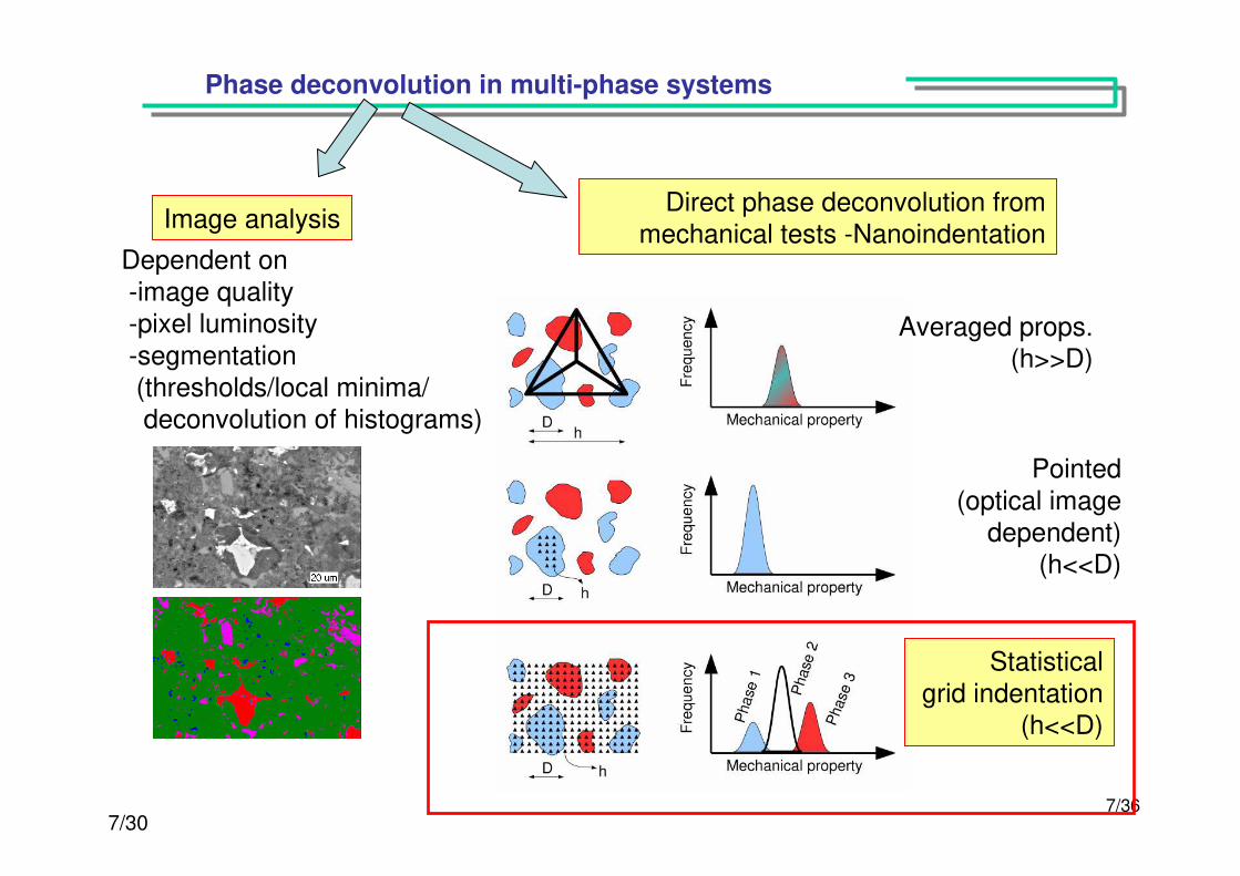
Phase deconvolution in multi-phase systems

Dependent on-image quality-pixel luminosity

-segmentation (thresholds/local minima/deconvolution of histograms)

Image analysisDirect phase deconvolution from

mechanical tests -Nanoindentation

Averaged props.(h>>D)

Pointed

(optical image dependent)

(h<<D)

Statisticalgrid indentation

(h<<D)

8/308/36

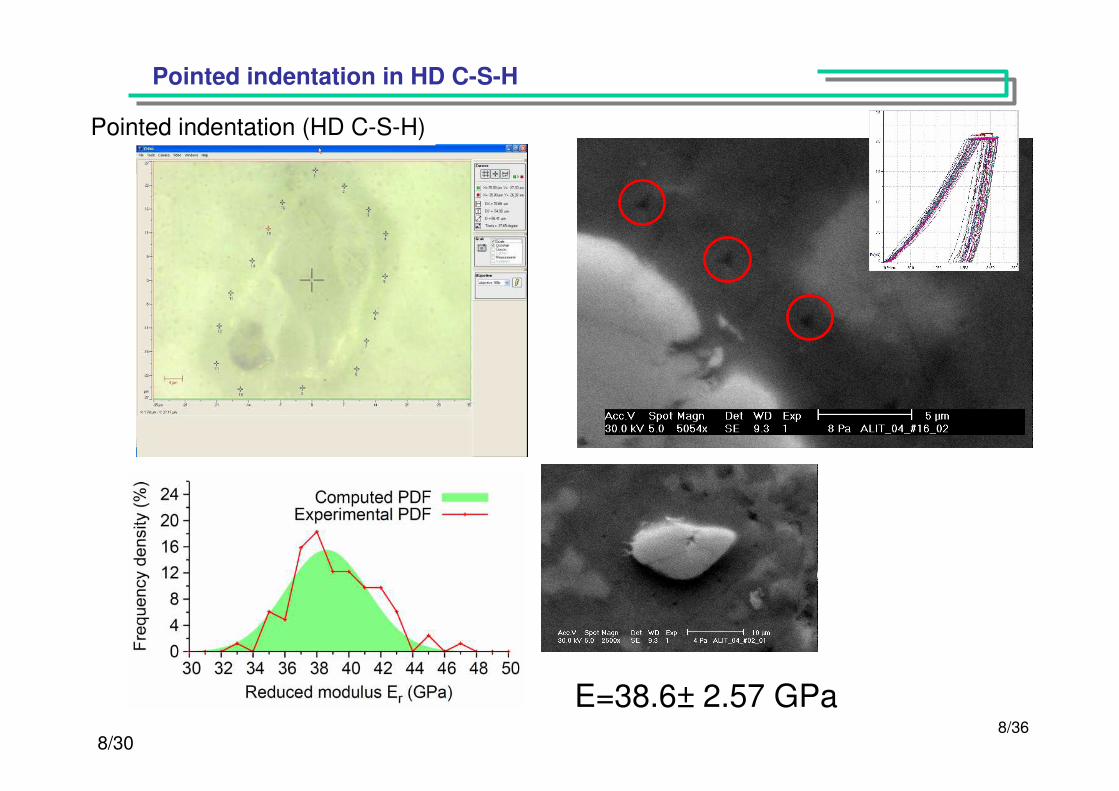
Pointed indentation in HD C-S-H

Pointed indentation (HD C-S-H)

E=38.6± 2.57 GPa

9/309/36

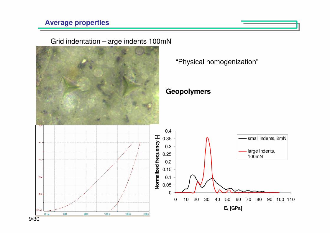
Average properties

Grid indentation –large indents 100mN

“Physical homogenization”

0

0.05

0.1

0.15

0.2

0.25

0.3

0.35

0.4

0 10 20 30 40 50 60 70 80 90 100 110

Er [GPa]

No

rma

lize

d f

req

ue

nc

y [

-] small indents, 2mN

large indents,100mN

Geopolymers

10/3010/36

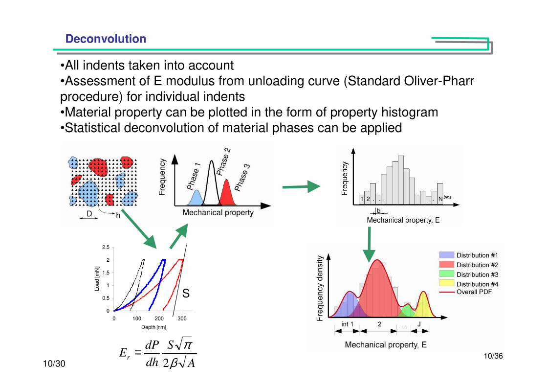
Deconvolution

A

S

dh

dPEr β

π2

=

0

0.5

1

1.5

2

2.5

0 100 200 300

Depth [nm]

Lo

ad

[m

N]

N-A-S-H

Partlyactivated

Fly ash

S

•All indents taken into account •Assessment of E modulus from unloading curve (Standard Oliver-Pharr procedure) for individual indents•Material property can be plotted in the form of property histogram•Statistical deconvolution of material phases can be applied

11/3011/36

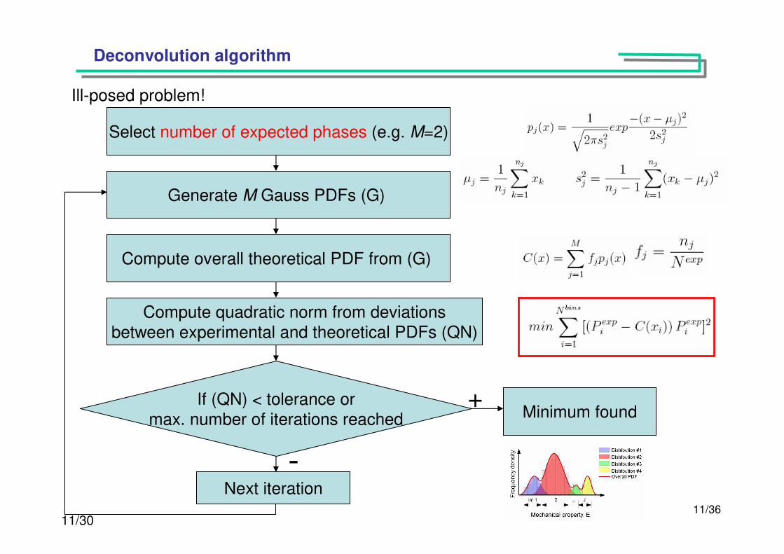
Deconvolution algorithm

Select number of expected phases (e.g. M=2)

Generate M Gauss PDFs (G)

Compute overall theoretical PDF from (G)

Compute quadratic norm from deviationsbetween experimental and theoretical PDFs (QN)

If (QN) < tolerance ormax. number of iterations reached Minimum found

Next iteration

+

-

Ill-posed problem!

12/3012/36

Nanoindentation on cement paste

Main phases at micro-scale•C-S-H gels (low and high density)•Portlandite Ca(OH)2

•Residual clinker•Capillary porosity

13/3013/36.

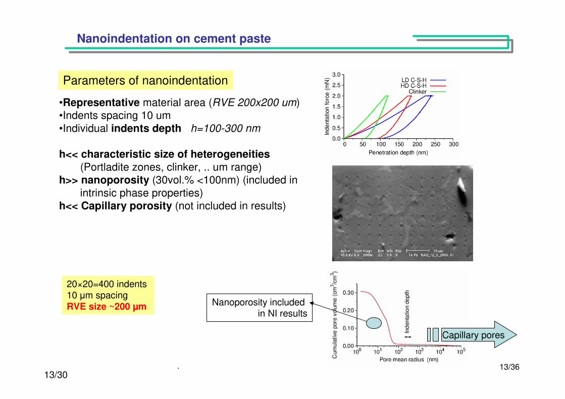
Nanoindentation on cement paste

•Representative material area (RVE 200x200 um)

•Indents spacing 10 um

•Individual indents depth h=100-300 nm

h<< characteristic size of heterogeneities(Portladite zones, clinker, .. um range)

h>> nanoporosity (30vol.% <100nm) (included in

intrinsic phase properties)

h<< Capillary porosity (not included in results)

Parameters of nanoindentation

Capillary pores

Nanoporosity included in NI results

20×20=400 indents10 µm spacing RVE size ~200 µm

14/3014/36

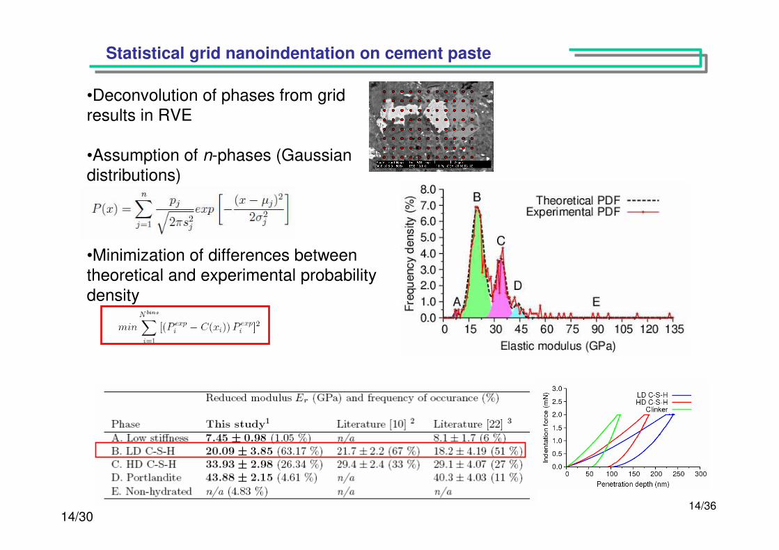
Statistical grid nanoindentation on cement paste

•Deconvolution of phases from grid results in RVE

•Assumption of n-phases (Gaussian distributions)

•Minimization of differences between theoretical and experimental probability

density

15/3015/36

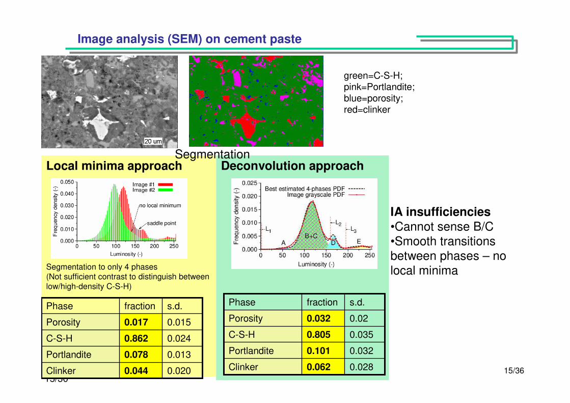
Deconvolution approachLocal minima approach

Image analysis (SEM) on cement paste

Segmentation to only 4 phases(Not sufficient contrast to distinguish between low/high-density C-S-H)

s.d.fractionPhase

0.044

0.078

0.862

0.017

0.020Clinker

0.013Portlandite

0.024C-S-H

0.015Porosity

green=C-S-H;pink=Portlandite;blue=porosity;red=clinker

s.d.fractionPhase

0.062

0.101

0.805

0.032

0.028Clinker

0.032Portlandite

0.035C-S-H

0.02Porosity

IA insufficiencies•Cannot sense B/C•Smooth transitions between phases – no local minima

Segmentation

16/3016/36

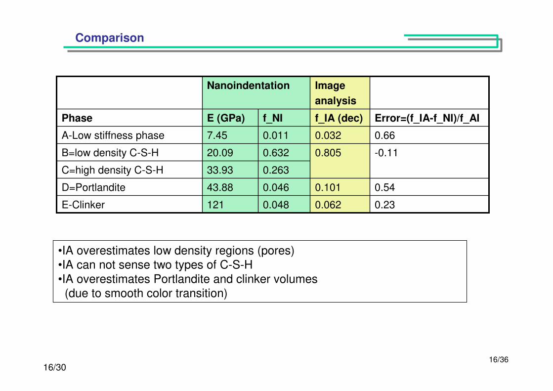
Comparison

Image

analysis

Nanoindentation

0.062

0.101

0.805

0.032

f_IA (dec)

0.23

0.54

-0.11

0.66

Error=(f_IA-f_NI)/f_AI

0.048

0.046

0.263

0.632

0.011

f_NIE (GPa)Phase

43.88D=Portlandite

121E-Clinker

33.93C=high density C-S-H

20.09B=low density C-S-H

7.45A-Low stiffness phase

•IA overestimates low density regions (pores)•IA can not sense two types of C-S-H

•IA overestimates Portlandite and clinker volumes(due to smooth color transition)

17/3017/36

Nanomechanical analysis of AAFA

18/3018/36

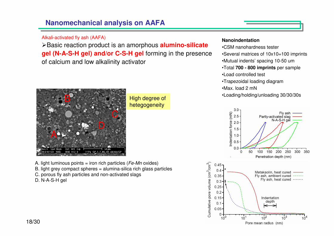
Nanomechanical analysis on AAFA

Alkali-activated fly ash (AAFA)

Basic reaction product is an amorphous alumino-silicate

gel (N-A-S-H gel) and/or C-S-H gel forming in the presence

of calcium and low alkalinity activator

A. light luminous points = iron rich particles (Fe-Mn oxides)B. light grey compact spheres = alumina-silica rich glass particlesC. porous fly ash particles and non-activated slagsD. N-A-S-H gel

B

A

CD

High degree of hetegogeneity

Nanoindentation

•CSM nanohardness tester

•Several matrices of 10x10=100 imprints

•Mutual indents’ spacing 10-50 um

•Total 700 - 800 imprints per sample

•Load controlled test

•Trapezoidal loading diagram

•Max. load 2 mN

•Loading/holding/unloading 30/30/30s

19/3019/36

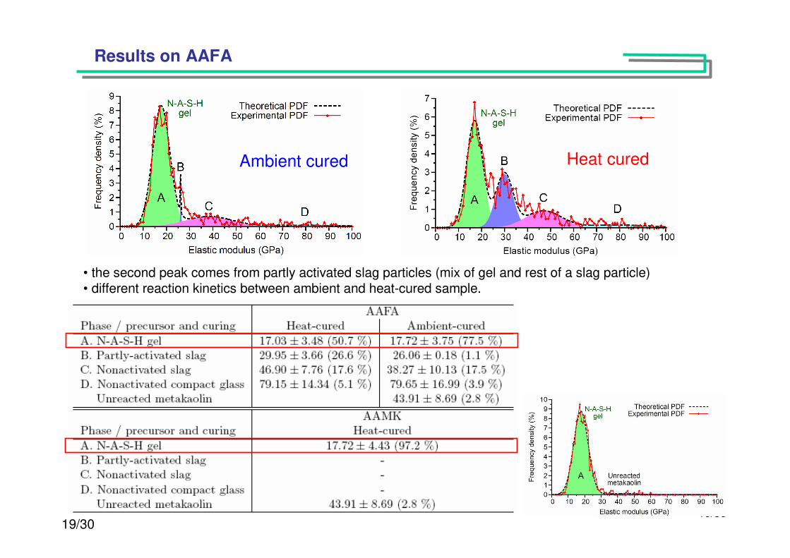
Results on AAFA

• the second peak comes from partly activated slag particles (mix of gel and rest of a slag particle)• different reaction kinetics between ambient and heat-cured sample.

Heat curedAmbient cured

20/3020/36

Nanomechanical analysis on gypsum

21/3021/36

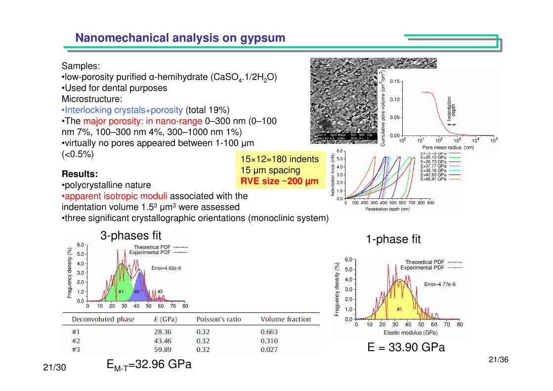
Nanomechanical analysis on gypsum

Samples:•low-porosity purified α-hemihydrate (CaSO4.1/2H2O)•Used for dental purposesMicrostructure:•Interlocking crystals+porosity (total 19%)•The major porosity: in nano-range 0–300 nm (0–100 nm 7%, 100–300 nm 4%, 300–1000 nm 1%)•virtually no pores appeared between 1-100 µm (<0.5%)

Results:•polycrystalline nature•apparent isotropic moduli associated with theindentation volume 1.53 µm3 were assessed•three significant crystallographic orientations (monoclinic system)

E = 33.90 GPa

3-phases fit 1-phase fit

15×12=180 indents15 µm spacing RVE size ~200 µm

EM-T=32.96 GPa

22/3022/36

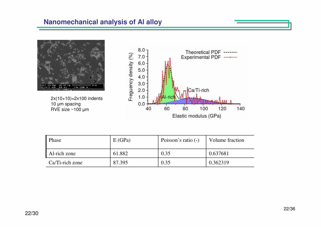
Nanomechanical analysis of Al alloy

2x(10×10)=2x100 indents10 µm spacing RVE size ~100 µm

0.3623190.3587.395Ca/Ti-rich zone

0.6376810.3561.882Al-rich zone

Volume fractionPoisson’s ratio (-)E (GPa)Phase

23/3023/36

Up-scaling low level properties to upper level

24/3024/36

Motivation

Structural materials (concrete, gypsum, plastics, wood, …) are characterized by

Multiscale heterogeneity (different chemical and mechanical phases)

Phase separation process (depends on scale nm-mm)

Micromechanics

mm-cmOverallproperties

Traditional concept

Characterization of individualcomponents and microstructure

RVE

Effective

(homogenized)properties

Material = black-box

Microstructure based evaluation

DLd <<<<

D

L

d

25/3025/36

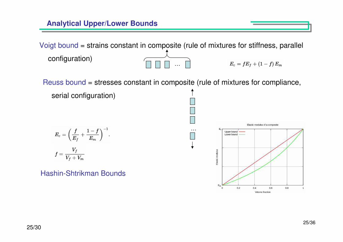
Analytical Upper/Lower Bounds

Voigt bound = strains constant in composite (rule of mixtures for stiffness, parallel

configuration)…

Reuss bound = stresses constant in composite (rule of mixtures for compliance,

serial configuration)

…

Hashin-Shtrikman Bounds

26/3026/36

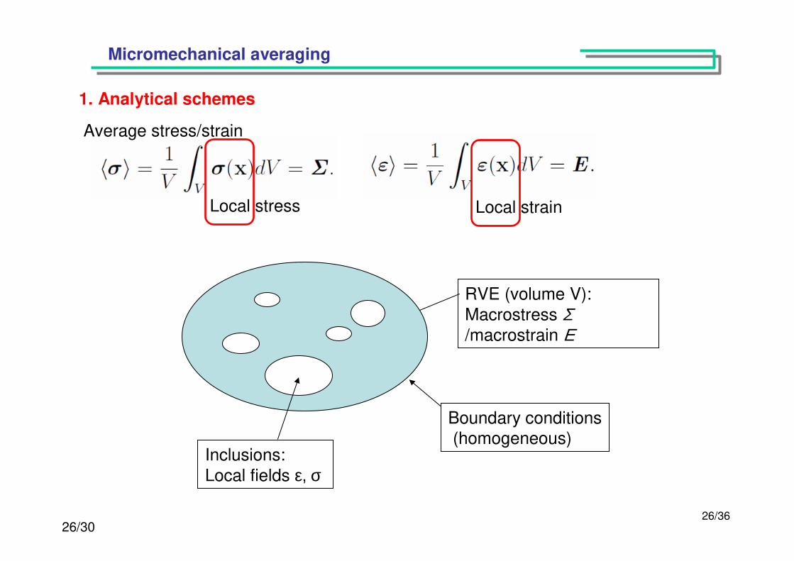
Micromechanical averaging

1. Analytical schemes

Average stress/strain

Local stress

RVE (volume V):

Macrostress Σ/macrostrain Ε

Boundary conditions(homogeneous)

Inclusions:

Local fields ε, σ

Local strain

27/3027/36

Micromechanical averaging

localstiffn

ess

and

com

plia

nce

ten

sors

stra

inor

stre

ss lo

caliz

atio

n

(concentra

tion)

tensors

r-phase medium:fr… volume fractioncr/sr…local stiffness/compliance tensors

Ar/Br… localization tensors

Eshelby’s estimate

For r-phases:

28/3028/36

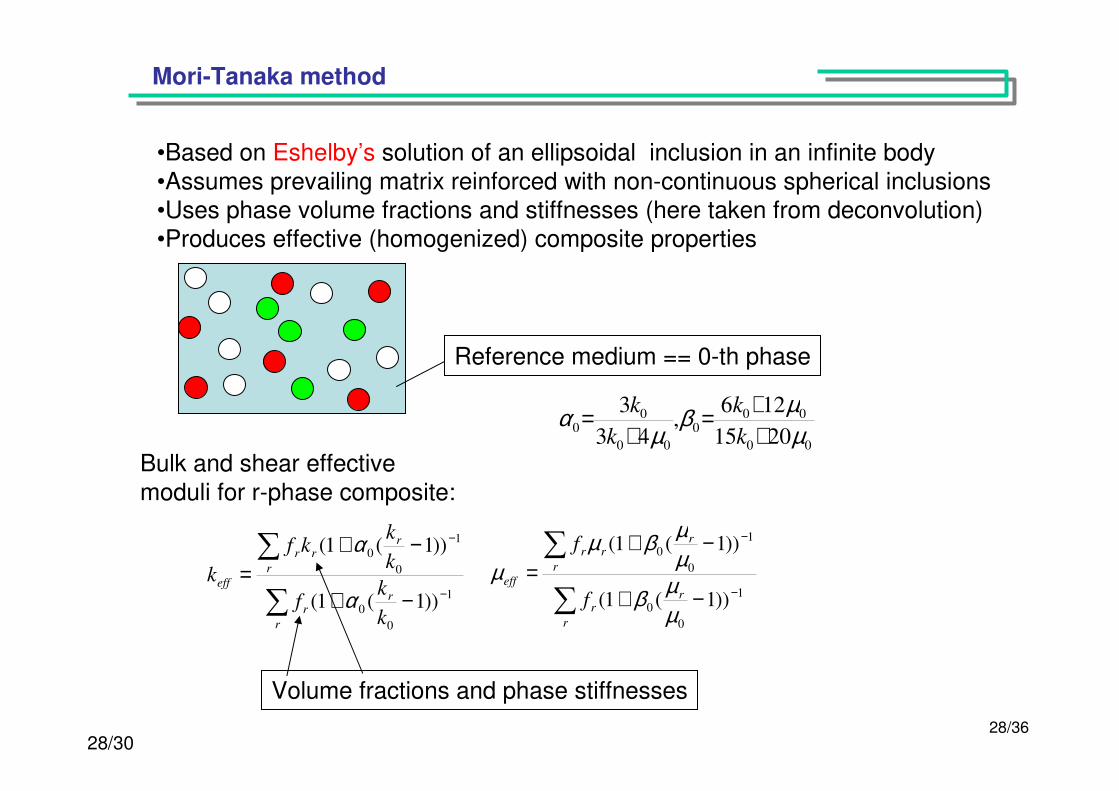
Mori-Tanaka method

∑

∑−

−

−+

−+=

r

rr

r

rrr

eff

k

kf

k

kkf

k1

0

0

1

0

0

))1(1(

))1(1(

α

α

∑

∑−

−

−+

−+=

r

rr

r

rrr

eff

f

f

1

0

0

1

0

0

))1(1(

))1(1(

µµβ

µµβµ

µ

00

000

00

00

2015

126,

43

3

µµβ

µα

++=

+=

k

k

k

k

Bulk and shear effective

moduli for r-phase composite:

Reference medium == 0-th phase

Volume fractions and phase stiffnesses

•Based on Eshelby’s solution of an ellipsoidal inclusion in an infinite body

•Assumes prevailing matrix reinforced with non-continuous spherical inclusions•Uses phase volume fractions and stiffnesses (here taken from deconvolution)•Produces effective (homogenized) composite properties

29/3029/36

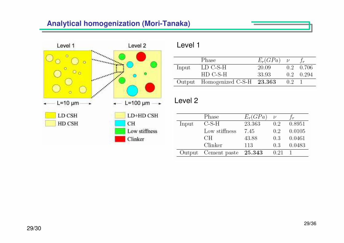
Analytical homogenization (Mori-Tanaka)

Level 1

Level 2

30/3030/36

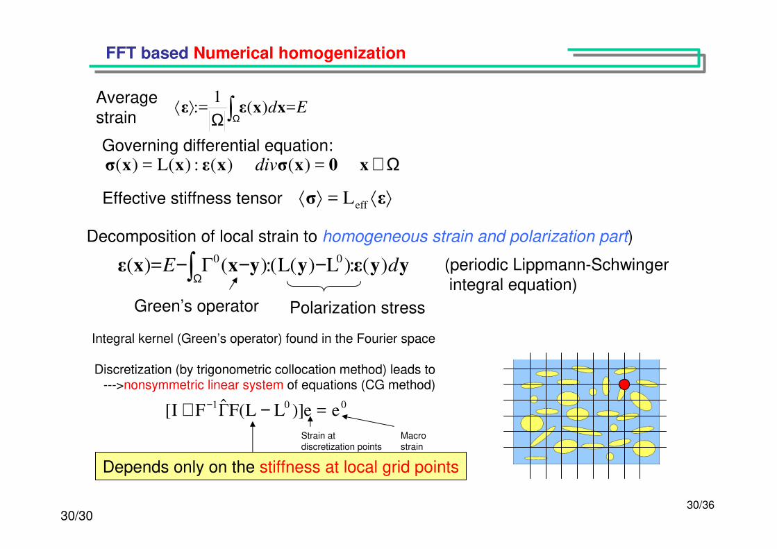
FFT based Numerical homogenization

Ed =)(1

:= xxεε ∫ΩΩ⟩⟨

Ω∈x0xσxεxxσ =)( )(:)(L=)( div

⟩⟨⟩⟨ εσ effL=

Governing differential equation:

yyεyyxxε dE )(:)L)(L(:)(Γ=)( 00 −−−∫ΩDecomposition of local strain to homogeneous strain and polarization part)

001 e=e)]LL(FΓFI[ −+ −

Average

strain

Effective stiffness tensor

Depends only on the stiffness at local grid points

Green’s operator Polarization stress

(periodic Lippmann-Schwingerintegral equation)

Strain at

discretization points

Macro

strain

Integral kernel (Green’s operator) found in the Fourier space

Discretization (by trigonometric collocation method) leads to--->nonsymmetric linear system of equations (CG method)

31/3031/36

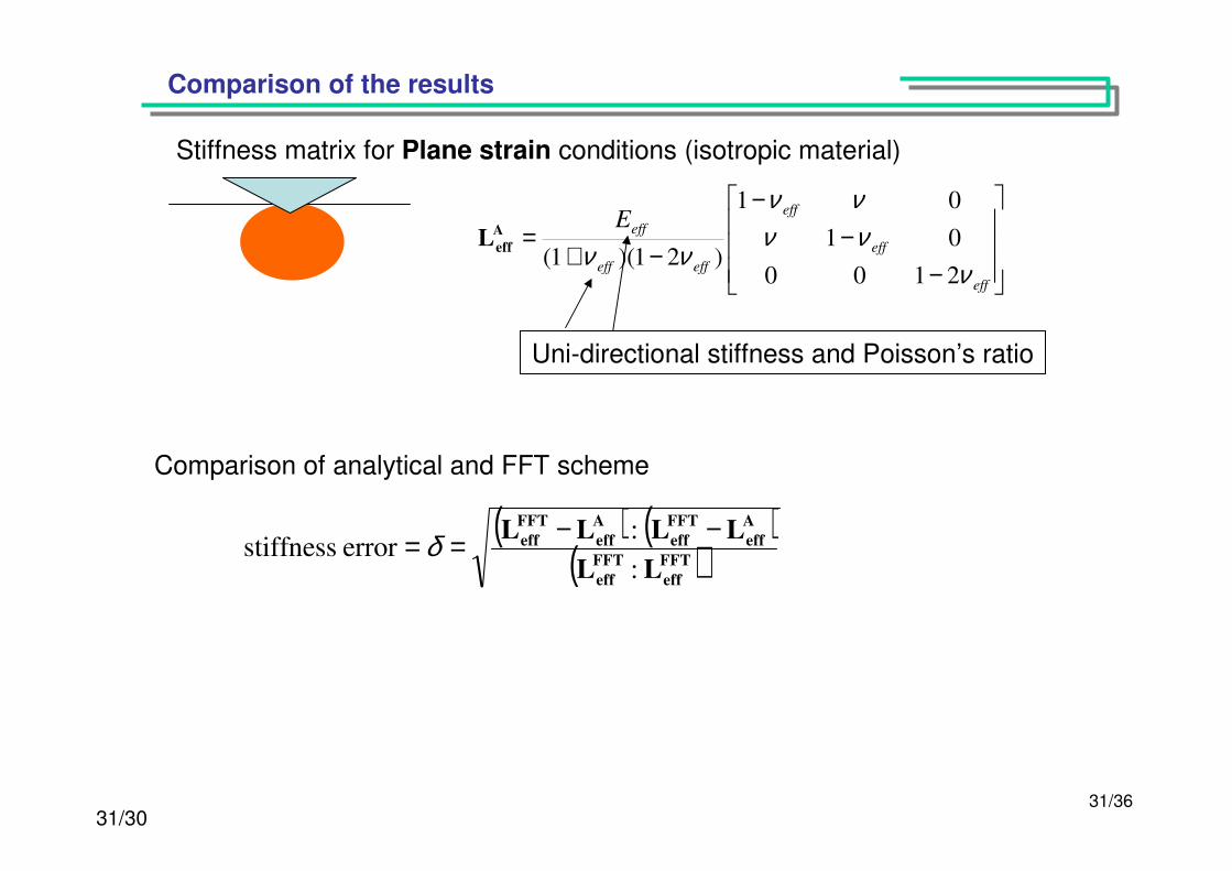
Comparison of the results

Comparison of analytical and FFT scheme

−−

−

−+=

eff

eff

eff

effeff

effE

ννννν

νν2100

01

01

)21)(1(

A

effL

Stiffness matrix for Plane strain conditions (isotropic material)

( ) ( )( )FFT

eff

FFT

eff

A

eff

FFT

eff

A

eff

FFT

eff

LL

LLLL

:

:error stiffness

−−== δ

Uni-directional stiffness and Poisson’s ratio

32/3032/36

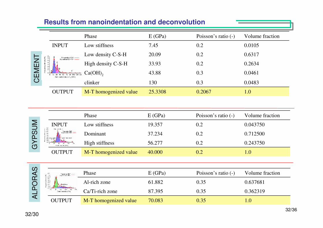
Results from nanoindentation and deconvolution

1.00.206725.3308M-T homogenized valueOUTPUT

0.04830.3130clinker

0.04610.343.88Ca(OH)2

0.26340.233.93High density C-S-H

0.63170.220.09Low density C-S-H

0.01050.27.45Low stiffnessINPUT



0.2437500.256.277High stiffness

0.7125000.237.234Dominant

0.0437500.219.357Low stiffnessINPUT



0.3623190.3587.395Ca/Ti-rich zone

0.6376810.3561.882Al-rich zoneINPUT


CE

ME

NT

GY

PS

UM

ALP

OR

AS

33/3033/36

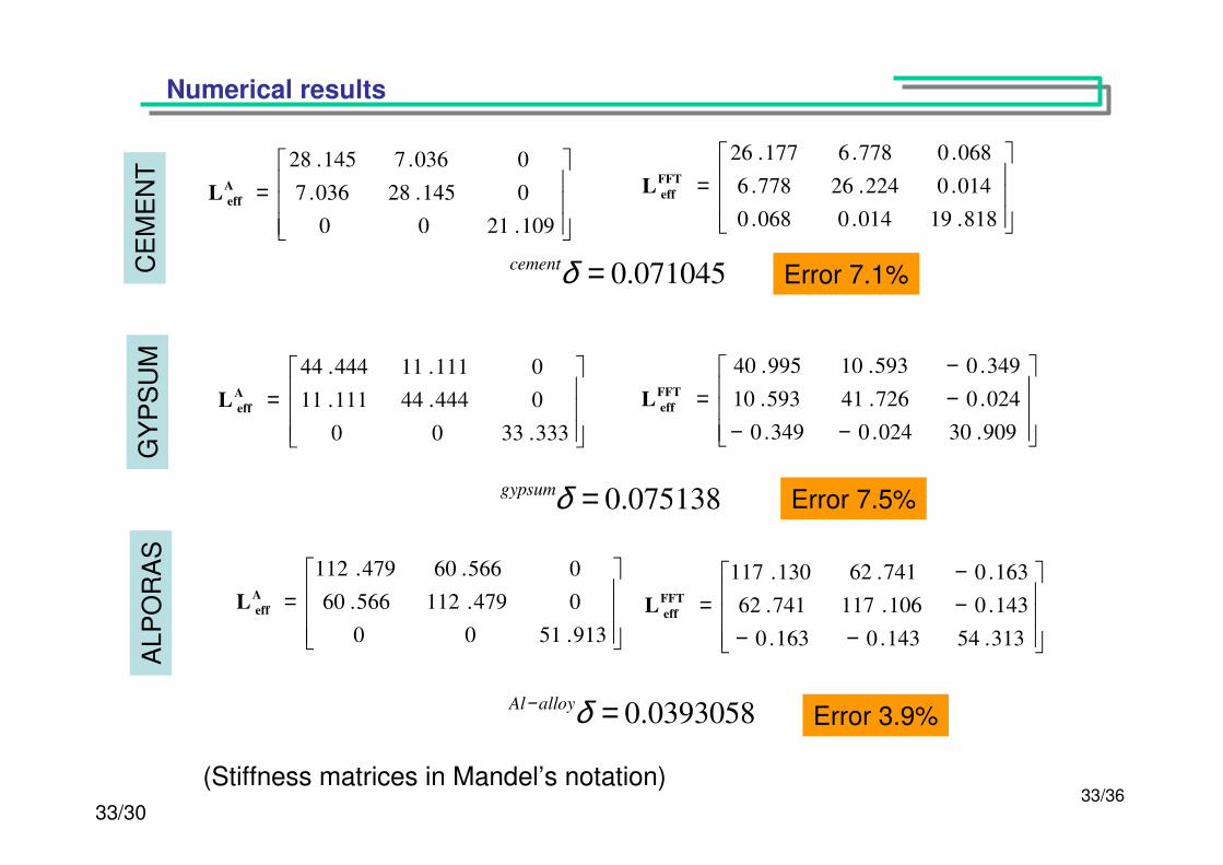
Numerical results

=109.2100

0145.28036.7

0036.7145.28A

effL

=818.19014.0068.0

014.0224.26778.6

068.0778.6177.26FFT

effL

=333.3300

0444.44111.11

0111.11444.44A

effL

−−−−

=909.30024.0349.0

024.0726.41593.10

349.0593.10995.40FFT

effL

=913.5100

0479.112566.60

0566.60479.112A

effL

−−−−

=313.54143.0163.0

143.0106.117741.62

163.0741.62130.117FFT

effL

0.071045=δcement

0.075138=δgypsum

0393058.0=− δalloyAl

CE

ME

NT

GY

PS

UM

ALP

OR

AS

Error 7.1%

Error 7.5%

Error 3.9%

(Stiffness matrices in Mandel’s notation)

34/3034/36

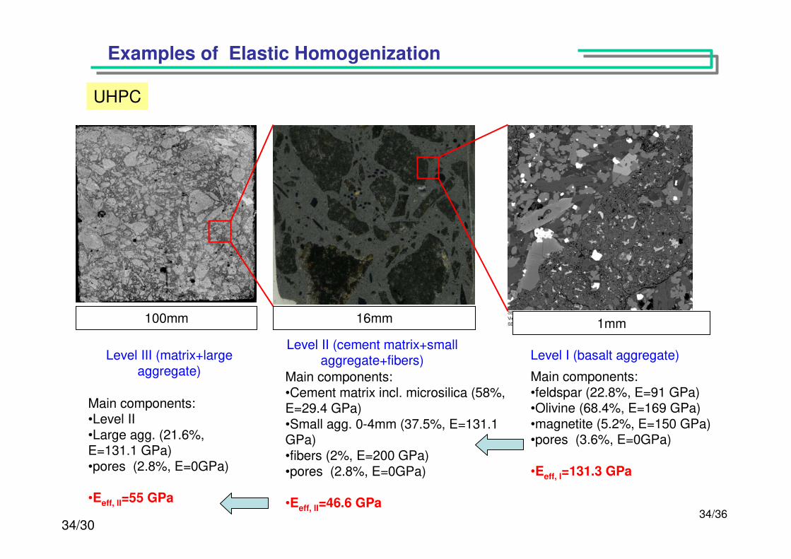
Examples of Elastic Homogenization

UHPC

16mm100mm

Level I (basalt aggregate)Level II (cement matrix+small

aggregate+fibers)Level III (matrix+largeaggregate) Main components:

•feldspar (22.8%, E=91 GPa)•Olivine (68.4%, E=169 GPa)•magnetite (5.2%, E=150 GPa)•pores (3.6%, E=0GPa)

•Eeff, I=131.3 GPa

Main components:•Cement matrix incl. microsilica (58%, E=29.4 GPa)•Small agg. 0-4mm (37.5%, E=131.1 GPa)•fibers (2%, E=200 GPa)•pores (2.8%, E=0GPa)

•Eeff, II=46.6 GPa

Main components:•Level II•Large agg. (21.6%, E=131.1 GPa)•pores (2.8%, E=0GPa)

•Eeff, II=55 GPa

1mm

35/3035/36

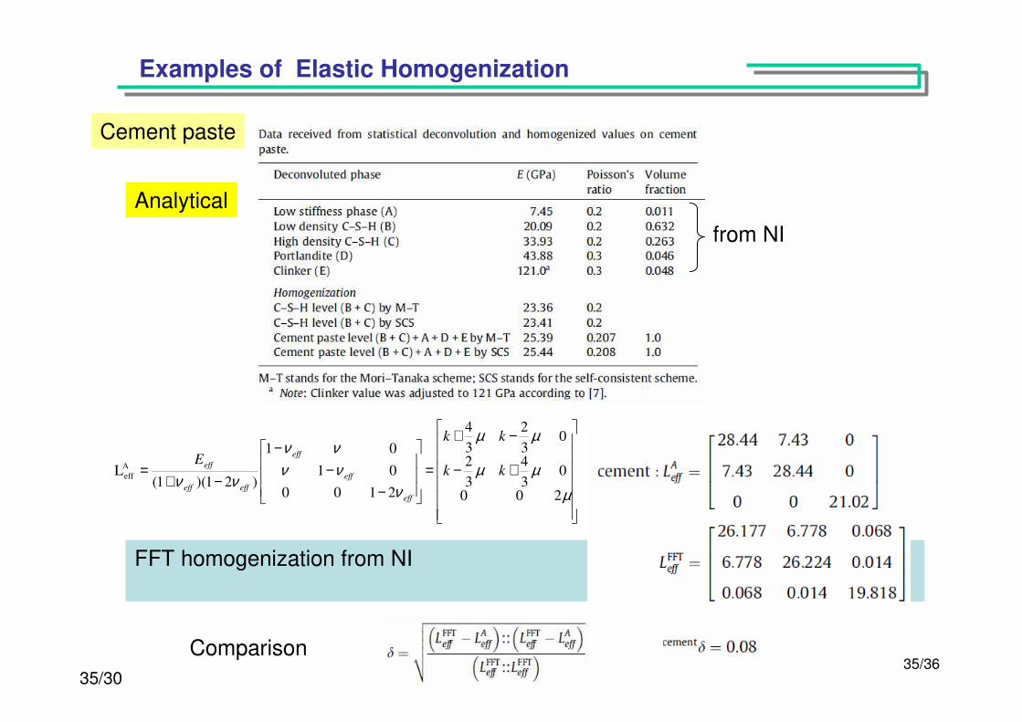
Examples of Elastic Homogenization

+−

−+

=

−−

−

−+=

µµµ

µµ

ννννν

νν200

03

4

3

2

03

2

3

4

2100

01

01

)21)(1(LA

eff kk

kk

E

eff

eff

eff

effeff

eff

Cement paste

from NI

FFT homogenization from NI

Analytical

Comparison

36/3036/36

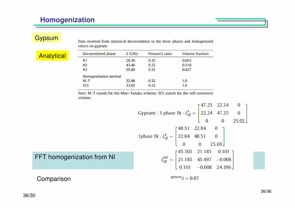
FFT homogenization from NI

Homogenization

Gypsum

Analytical

Comparison

Documents

Principy nanomechanické analýzy heterogenních materiálů