Private Information and a Macro Model of Exchange Rates:

Evidence from a Novel Data Set

Menzie D. Chinn*

University of Wisconsin, Madison

and NBER

and

Michael J. Moore**

Queen’s University, Belfast,

Northern Ireland, United Kingdom

This Version: July 3, 2008

Abstract

We propose an exchange rate model which is a hybrid of the conventional

specification with monetary fundamentals and the Evans-Lyons microstructure

approach. It argues that the failure of the monetary model is principally due to

private preference shocks which render the demand for money unstable. These shocks

to liquidity preference are revealed through order flow. We estimate a model

augmented with order flow variables, using a unique data set: almost 100 monthly

observations on inter-dealer order flow on dollar/euro and dollar/yen. The augmented

macroeconomic, or “hybrid”, model exhibits out of sample forecasting improvement

over the basic macroeconomic and random walk specifications.

JEL classification: D82; E41; F31; F47 Keywords: Exchange rates; Monetary model; Order flow; Microstructure; Forecasting performance * Corresponding author: Robert M. LaFollette School of Public Affairs; and Department of Economics, University of Wisconsin, 1180 Observatory Drive, Madison, WI 53706- 1393. Email: mchinn@lafollette.wisc.edu . ** Queens University School of Management, Queens University of Belfast, 25 University Square, Belfast BT7 1NN. United Kingdom . Email: m.moore@qub.ac.uk . We are grateful for the comments of our discussant Martin Evans and other participants at the Conference on International Macro Finance - April 24-25, 2008 at the International Monetary Fund, Washington D.C.

1

1. Introduction

One of the most enduring problems in international economics is the ‘exchange rate

disconnect’ puzzle. Numerous structural or arbitrage approaches have been tried.

Prominent among them are:

a) the sticky price monetary model

b) the Balassa-Samuelson model

c) the portfolio balance model

d) purchasing power parity

e) uncovered interest parity.

The in-sample and forecasting goodness of fit of these models were evaluated by

Cheung, Chinn and Garcia Pascual (2005 (a) and (b)). Their conclusions are not

unfamiliar:

“the results do not point to any given model/specification combination as being very successful. On the other hand, some models seem to do well at certain horizons, for certain criteria. And indeed, it may be that one model will do well for one exchange rate, and not for another.”

Recently, Gourinchas and Rey (2007) have used the external budget constraint to

devise a sophisticated measure of external imbalance which has forecasting power for

exchange rate changes over some horizons.1 However, the framework seems to be

limited to some of the institutional features of the US dollar and is ex-ante silent on

the timing and the composition of external adjustment between price and quantity.

The most theoretically and empirically startling innovation in the literature has been

the introduction of a finance microstructure concept – order flow – to explain

1 See an extended analysis on bilateral exchange rates using this framework in Alquist and Chinn (2008).

2

exchange rate movements. In a series of papers Evans and Lyons2 (2002, 2005,

2008), have shown that order flow contemporaneously explains a significant

proportion of the high-frequency variation in exchange rates. Evans (2008) is

particularly close to this paper in its emphasis on the importance of integrating

macroeconomics with the microstructure approach. Though their theoretical

framework is also very convincing, it has been difficult to evaluate its merit at

standard macroeconomic frequencies because of the proprietary nature of the data.

This paper fills this gap as it presents results on almost 100 monthly observations of

order flow nested within a conventional framework3.

In Section 2 we discuss the theoretical motivation for the hybrid monetary

fundamentals-order flow model we adopt. In Section 3 we outline the characteristics

of the data we employ in this study. Section 4 replicates the Evans and Lyons (2002)

results at the monthly frequency, confirming the fact that the order flow data we use

(and the sample period examined) are representative. Our empirical methodology and

basic in-sample results are discussed in Section 5. The next section reports some of

the robustness tests implemented. Section 7 reports the preliminary results of our out-

of-sample validation exercises that demonstrate the predictive power of the hybrid

model. The final section makes some concluding remarks.

2 These are just examples of their work. For a fuller account, see http://www9.georgetown.edu/faculty/evansm1/Home%20page.htm 3 Berger et al. (2006) also obtained access to a long run of EBS order flow data. – 6 years from 1999 to 2004 but they do not integrate this into the conventional monetary analysis.

3

2. Theoretical Background

2.1 The Representative Agent

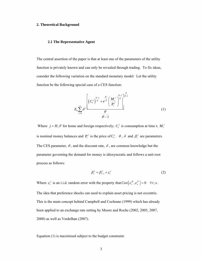
The central assertion of the paper is that at least one of the parameters of the utility

function is privately known and can only be revealed through trading. To fix ideas,

consider the following variation on the standard monetary model: Let the utility

function be the following special case of a CES function:

( )1 1

1

00

1

jt j

j tt j

tt

t

MC eP

E

θθ θβθ θ

θθ

δ θθ

− −−

∞

=

⎡ ⎤⎛ ⎞⎢ ⎥+ ⎜ ⎟⎢ ⎥⎝ ⎠⎢ ⎥⎣ ⎦

−

∑ (1)

Where ,j H F= for home and foreign respectively; jtC is consumption at time t; j

tM

is nominal money balances and jtP is the price of j

tC . θ , δ and jtβ are parameters.

The CES parameter, θ , and the discount rate, δ , are common knowledge but the

parameter governing the demand for money is idiosyncratic and follows a unit root

process as follows:

1j j j

t t tβ β ε−= + (2)

Where jtε is an i.i.d. random error with the property that ( ), 0 ,H F

r sCov r sε ε = ∀ .

The idea that preference shocks can used to explain asset pricing is not eccentric.

This is the main concept behind Campbell and Cochrane (1999) which has already

been applied to an exchange rate setting by Moore and Roche (2002, 2005, 2007,

2008) as well as Verdelhan (2007).

Equation (1) is maximised subject to the budget constraint:

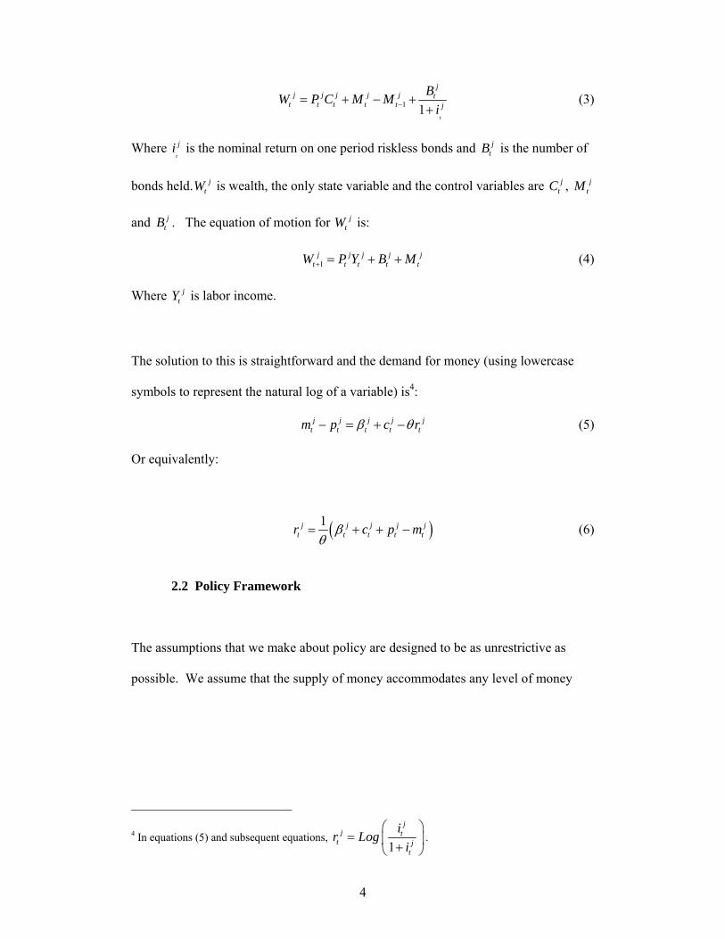
4

1 1t

jj j j j j t

t t t t t j

BW P C M Mi−= + − +

+ (3)

Where t

ji is the nominal return on one period riskless bonds and jtB is the number of

bonds held. jtW is wealth, the only state variable and the control variables are j

tC , jtM

and jtB . The equation of motion for j

tW is:

1j j j j j

t t t t tW P Y B M+ = + + (4)

Where jtY is labor income.

The solution to this is straightforward and the demand for money (using lowercase

symbols to represent the natural log of a variable) is4:

j j j j jt t t t tm p c rβ θ− = + − (5)

Or equivalently:

( )1j j j j jt t t t tr c p mβ

θ= + + − (6)

2.2 Policy Framework

The assumptions that we make about policy are designed to be as unrestrictive as

possible. We assume that the supply of money accommodates any level of money

4 In equations (5) and subsequent equations, 1

jj t

t jt

ir Logi

⎛ ⎞= ⎜ ⎟+⎝ ⎠

.

5

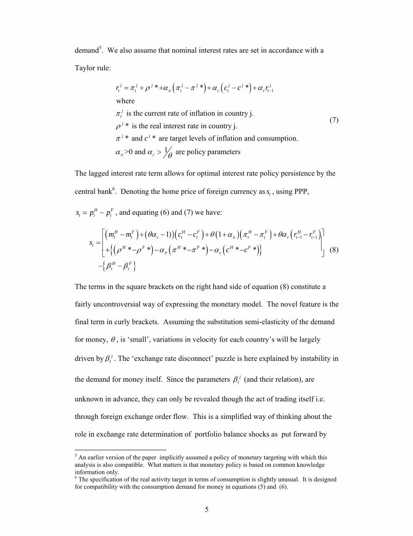
demand5. We also assume that nominal interest rates are set in accordance with a

Taylor rule:

( ) ( ) 1* * *

where is the current rate of inflation in country j.

* is the real interest rate in country j.* and * are target levels of inflation and consumption.

>0

j j j j j j j jt t t c t r t

jt

j

j j

r c c r

c

π

π

π ρ α π π α α

π

ρ

π

α

−= + + − + − +

1 and are policy parameterscα θ>

(7)

The lagged interest rate term allows for optimal interest rate policy persistence by the

central bank6. Denoting the home price of foreign currency as ts , using PPP,

H Ft t ts p p= − , and equating (6) and (7) we have:

( ) ( )( ) ( )( ) ( )( ) ( ) ( ){ }

{ }

1 11) 1

* * * * * *

H F H F H F H Ft t c t t t t r t t

t H F H F H Fc

H Ft t

m m c c r rs

c c

π

π

θα θ α π π θα

ρ ρ α π π α

β β

− −⎡ ⎤− + − − + + − + −⎢ ⎥=⎢ ⎥+ − − − − −⎣ ⎦

− −

(8)

The terms in the square brackets on the right hand side of equation (8) constitute a

fairly uncontroversial way of expressing the monetary model. The novel feature is the

final term in curly brackets. Assuming the substitution semi-elasticity of the demand

for money, θ , is ‘small’, variations in velocity for each country’s will be largely

driven by jtβ . The ‘exchange rate disconnect’ puzzle is here explained by instability in

the demand for money itself. Since the parameters jtβ (and their relation), are

unknown in advance, they can only be revealed though the act of trading itself i.e.

through foreign exchange order flow. This is a simplified way of thinking about the

role in exchange rate determination of portfolio balance shocks as put forward by

5 An earlier version of the paper implicitly assumed a policy of monetary targeting with which this analysis is also compatible. What matters is that monetary policy is based on common knowledge information only. 6 The specification of the real activity target in terms of consumption is slightly unusual. It is designed for compatibility with the consumption demand for money in equations (5) and (6).

6

Flood and Rose (1999). More specifically, shocks to liquidity demands is one of the

motivations offered for the link between order flow and exchange rate in the seminal

paper by Evans and Lyons (2002). The contention of this paper is that cumulative

shocks to liquidity demand, as specified by equation (2), are captured by cumulative

foreign exchange order flow. Bjonnes and Rime (2005) and Killeen, Lyons and

Moore (2006) provide evidence that exchange rate levels and cumulative order flow

are cointegrated in high frequency data. If equation (6) were correct, exchange rate

levels should be cointegrated with both cumulative order flow and the traditional

vector of ‘fundamentals’ of the monetary model at all frequencies. It has been

impossible to test this up to this point because of lack of data.

3. Data

The data is monthly from January 1999 to January 2007 (see the Data Appendix for

greater detail, and summary statistics). Two currency pairs are considered:

dollar/euro and dollar/yen.

The most novel aspect of the data is the long span of order flow data. That data was

obtained from Electronic Broking Services (EBS). This is one of the two major

global inter-dealer foreign exchange trading platforms. It dominates spot brokered

inter dealer trading in dollar/yen and is responsible for an estimated 90% of

dollar/euro business in the same category. The two series are:

• Order Flow: Monthly buyer initiated trades net of seller initiated trades, in

millions of base currency (OFEURUSD, OFUSDJPY)

• Order Flow Volume: Monthly sum of buyer-initiated trades and seller-initiated

trades, in millions of base currency.

7

For dollar/euro, the base currency is the euro while the dollar is the base currency for

dollar/yen. In the empirical exercise, we standardize the data by converting

OFEURUSD into dollar terms so that the order flow variable enters into each

equation analogously.7 In some of the robustness checks, the order flow variables are

normalized by volume (also adjusted into dollar terms). The raw order flow and order

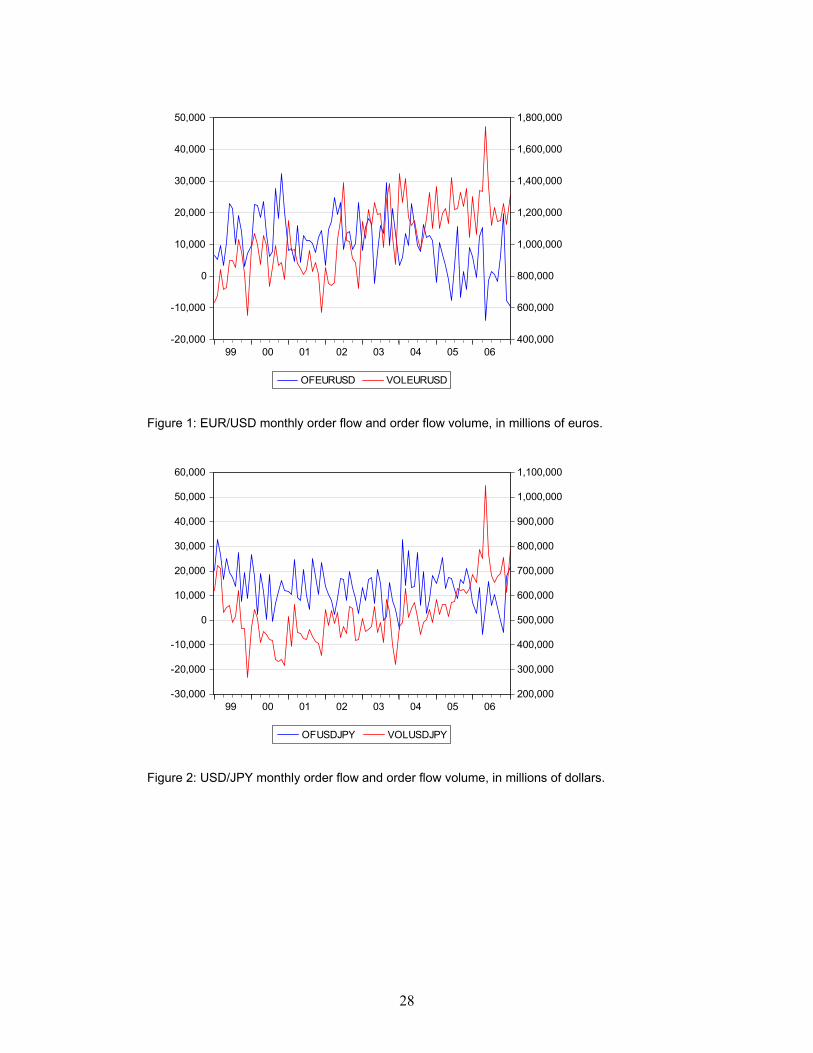
flow volume data are depicted in Figures 1 and 2.

A note of caution about the definition of order flow is worth entering at this point.

We follow the convention of signing a trade using the direction of the market order

rather than the limit order. For the current data set, this is carried out electronically by

EBS and we do not need to rely on approximate algorithms such as that proposed by

Lee and Ready (1991). The reason why the market order is privileged as the source

of information is that the trader foregoes the spread in favor of immediacy when she

hits the bid or takes the offer in a limit order book. Nevertheless, an informed trader

can optimally choose to enter a limit order rather than a market order though she is

less likely to do so. For a fuller discussion of this issue, see Hollifield, Miller and

Sandas (2004) and Parlour (1998).

The other data are standard. Monthly data were downloaded from the IMF’s

International Financial Statistics. The exchange rate data used for prediction are end-

of-month. The exchange rate data used to convert order flow, as well as the interest

rate data, are period average, which is most appropriate given the order flow data are

in flow terms. In our basic formulation, money is M2 (the ECB-defined M3 for Euro

7 OFUSDJPY is multiplied by a negative sign to generate the corresponding yen variable.

8

area), inflation is 1 month log-differenced CPI, annualized.8 Note that we proxy

consumption with industrial production (in logs), in line with standard practice.

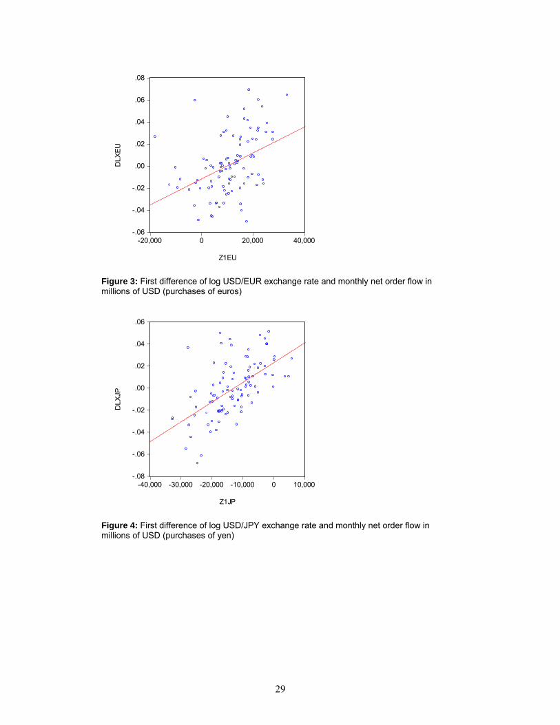
The key variables, the exchange rates and transformed order flow series are displayed

in Figures 3 and 4 for the dollar/euro and dollar/yen, respectively. Note that in these

graphs, the exchange rates are defined (dollar/euro and dollar/yen) and order flow

transformed so that the implied coefficient is positive.9

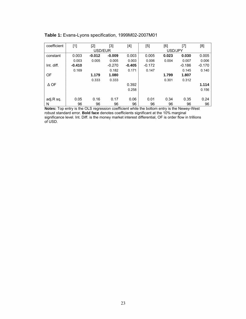
4. Replicating the Evans-Lyons Results

In order to verify that the results we obtain are not driven by any particular

idiosyncratic aspects of our data set, we first replicate the results obtained by Evans

and Lyons (2002). They estimate regressions of the form (7).

tttttt uofofiis +Δ++−+=Δ )()()( 32*

10 ββββ (7)

Where i are short term nominal interest rates and of is order flow. The estimates we

obtain are reported in Table 1. Several observations are noteworthy. First, the

proportion of variation explained goes up substantially when order flow in levels is

included.

Second, the interest differential coefficient is only statistically significant (with the

anticipated sign10) when the order flow variables are omitted, and then only in the

dollar/euro case. Inclusion of the order flow variables reduce the economic and

8 As noted in Section 6, we also check to see if the results are robust to use of M1 as a money variable, different inflation rates (3 month or twelve month differences of log-CPI), or real GDP (at the quarterly frequency). M1 and real GDP are also drawn from IFS. 9 Note that we have also run the regressions with the raw order flow and cumulative demeaned raw order flow data. The qualitative aspects of the regression results do not change – order flow remains important in both a statistical and economic sense. 10 The negative slope is consistent with a sticky price monetary model story, though not, of course with uncovered interest parity.

9

statistical significance of the interest rate differential in this case. In short, any

suspicion that the Evans-Lyons result is an artefact of high-frequency data is firmly

dispelled. The results are, however, consistent with those of Berger et al. (2006) who

argue that the Evans Lyons result is relatively weaker at lower frequencies.

5. Empirics

We implement the rest of the portion of the paper in the following manner.

a) The Johansen Procedure is applied to test for cointegration between the

exchange rates, cumulative order flow and model fundamentals (here taken to

be money, income, interest and inflation rates), as suggested by equation 8.

Notice that except for order flow, the macroeconomic variables of importance

are the same as those in the sticky price monetary model of exchange rates,

assuming the targets are constant.

b) The dynamic OLS procedure of Stock and Watson (2003) is used to obtain the

long run coefficients.

c) The implied error correction model is estimated.

d) Out of sample forecasts for different models are compared

5.1 Testing for Cointegration

The first step in the cointegration test procedure is to determine the optimal lag

length. We evaluated the VAR specifications implied by the basic model and the basic

model augmented by the order flow variable (in this case cumulated). We term this

latter version the “hybrid” model. Note that we de-mean the order flow data, so that

we remove a deterministic time trend from the cumulative order flow series.

10

The Akaike Information Criterion typically selects a fairly short lag length of one or

two lags in the VAR specification. However, these specifications also typically

exhibit substantial serial correlation in the residuals, according to inspection of the

autocorrelograms up to lag 12. In contrast, the residuals appear serially uncorrelated

when four lags are included in the VARs. Hence, we opt to fix on the four lag

specification.11

We applied the Johansen (1988) maximum likelihood procedure to confirm that the

presence of cointegration, and to account for the possibility of multiple cointegrating

vectors. Table 2 reports the results of our tests.

The first three columns of Table 2 pertain to specifications including only monetary

fundamentals (money, income, interest and inflation rates). Columns 4-6 pertain to the

basic model augmented with cumulative order flow. Columns [1] and [4] pertain to

model specifications allowing a constant in the cointegrating equation, columns [2]

and [5] to ones allowing a constant in both the cointegrating equation, and in the

VAR, and columns [3] and [6] allowing intercept and trend in the cointegrating

equation, and a constant in the VAR (in all but columns [1] and [4], deterministic time

trends are allowed in the data).

The numbers pertain to the implied number of cointegrating vectors using the trace

and maximal eigenvalue statistics (e.g., “2,1” indicates the trace and maximal

eigenvalue statistics indicate 2 and 1 cointegrating vectors, respectively). Since the

number of observations is not altogether large relative to the number of coefficients

11 Only in the USD/JPY hybrid model case does a 3 lag specification appear plausible. To maintain consistency across specifications, we retain the four lag specification in all cases.

11

estimated in the VARs, we also report the results obtained when using the adjustment

to obtain finite sample critical values suggested by Cheung and Lai (1993). Hence,

“Asy” entries denote results pertaining to asymptotic critical values, and “fs”, to finite

sample critical values.

Inspection of Table 2 confirms that that it is fairly easy to find evidence of

cointegration using the 5% marginal significance level. The specification selected by

the AIC for the basic model is one that omits a constant in the VAR equation for the

dollar/euro, and one including a constant in both the cointegrating vector and the

VAR for the dollar/yen. In the case of the hybrid model, there is again some diversity

of results. For the dollar/euro, there seems to be some argument for no trend in the

cointegrating relationship, while a trend appears in the cointegrating vector for the

dollar/yen.

Table 2 also indicates that it is quite easy to obtain evidence of cointegration – and

indeed cointegration with multiple long run relationships – using the asymptotic

critical values. We opt to put greater weight on the finite sample critical values.

The resulting results are highly suggestive that there is one cointegrating vector in

almost all cases; we proceed accordingly.12 This conclusion points to an important

role for cumulative order flow in determining long term exchange rates but only in

combination with monetary fundamentals.

12 Note that while we could rely upon the Johansen procedure to obtain estimates of the long run and short run coefficients, we decided to rely upon the DOLS procedure, in large part because the estimates we obtained via this method were so implausibly large, and sensitive to specification. In addition, Stock and Watson (1993) present simulation results that indicate that DOLS estimates are less dispersed than Johansen estimates.

12

5.2 Estimating the Long Run Relationships and the Error Correction Models

We estimate the cointegrating relationship using dynamic OLS (Stock and Watson,

1993), which is appropriate if there is one cointegrating vector. The procedure

involves running a regression involving two leads and lags of first differences of the

right hand side variables.

ti ittt uBXXs +Δ++Γ= ∑+

−= +2

2δτ (8)

Where X is a vector of monetary fundamentals and cumulative order flow, τ is a time

trend (which is suppressed in some specifications). Using these estimates, error

correction terms are defined thus:

))ˆˆ(( τδ+Γ−= ttt XsECT (9)

And then incorporated into single equation error correction models.13

tttt vECTXs ++Δ=Δ −− 11 ϕ (10)

Where φ should take on a negative value, significantly different from zero, if the

exchange rate responds to disequilibria in the fundamentals.

In the results that are reported, a standardized specification incorporating one lag of

first differenced monetary fundamentals, is used. One could adopt a general-to-

specific methodology with the objective of identifying a parsimonious specification.

Typically, such an approach leads to error correction models with short lags (a lag or

at most two of first differenced terms), with perhaps income and inflation variables

omitted. In order to maintain consistency of specifications across models, we opt to

present the results of models incorporating only one lag of the differenced monetary

fundamentals.

13 In some specifications, order flow is entered in contemporaneously, including the one that incorporates cumulative order flow in the cointegrating relationship.

13

5.3 Long- and Short-Run Coefficients

The results of estimating these equations for the dollar/euro and dollar/yen are

reported in Tables 3 and 4, respectively.14 Turning first to Table 3, columns [1]-[3],

one finds little evidence that the exchange rate reacts to the long run monetary

fundamentals (note that while order flow is included in columns [2] and [3],

cumulative order flow is not included in the cointegrating relation). So order flow is

clearly important in determining the rate of exchange rate depreciation (notice that the

adjusted R-squared rises from 1% to 26%).

The cointegration tests suggest that cumulative order flow does enter into the

cointegrating relationship. The specification in column [4] conforms to that

specification. Allowing the cumulative order flow to enter into the long run

relationship, and order flow into the short run relationship, explains a large proportion

of variation in the exchange rate change (25%). In addition, the cumulative order flow

variable is very significant.15

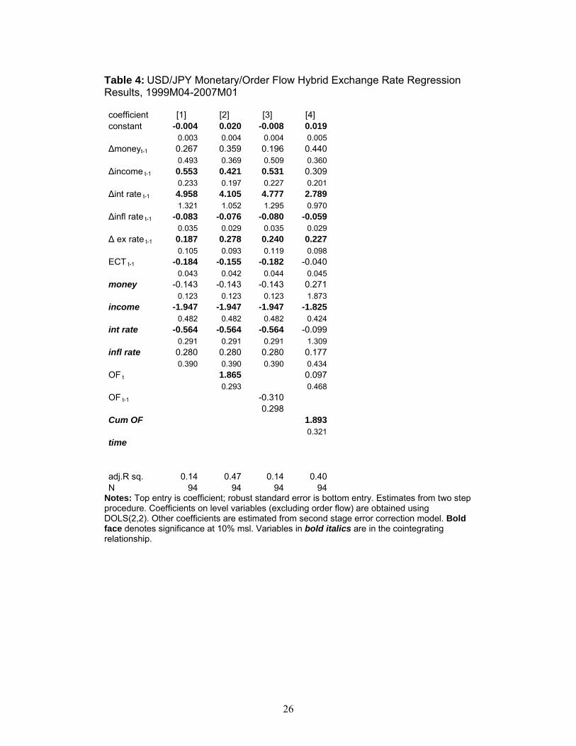
Turning to the dollar/yen results in Table 4, one observes that the monetary

fundamentals do seem to be important in the long run (column [1]); the error

correction term coefficient is statistically significant and negative as expected.

However, inclusion of contemporaneous order flow increases the adjusted R2

substantially, from 0.14 to 0.47. Lagged order flow has no similar impact.

14 We rely upon a single equation estimation methodology focused on the exchange rate as the dependent variable, which is appropriate if the “fundamentals” are weakly exogenous. We tested for this condition, and this is typically the case, especially when inflation is measured as the three month change. 15 Although the exchange rate does not respond in an economically and statistically significant way to disequilibria as measured by the error correction term, we will still examine if inclusion of the ECT helps in prediction.

14

Cumulative (demeaned) order flow also appears important for the long run behaviour

of the exchange rate (column [4]), although when cumulative order flow is included at

the same time as the contemporaneous order flow variable, the proportion of variation

adjusted for degrees of freedom is lower than in column [2].

To sum up the results from this section, there does appear to be significant evidence

of a long run relationship between exchange rates and monetary fundamentals

augmented by cumulative order flow. Even when cumulative order flow might be

argued to not enter into the long run relationship (i.e., in the case of the dollar/yen), it

is clear that order flow always enters into the short run relation.

6. Robustness Tests

We have investigated a number of variations to the basic specifications, to check

whether the empirical results are robust.

• Order flow vs. normalized order flow

• M1 vs M2

• 3 month vs. 1 month inflation

• Quarterly vs. monthly data

We deal with each of these issues in turn.

Order flow issues. The order flow variables are included in dollar terms. It is

reasonable to scale net order flow variable by the volume of order flow. The results in

the Evans and Lyons regressions are basically unchanged. Using this normalized

order flow variable in the hybrid model specifications (conforming to columns [2]-[3]

15

and [6]-[7] in Tables 3 and 4) does not result in any appreciable change in the

results.16

Money measures. While the substitution of narrow money for M2 results in slightly

different results, particularly with respect to the short- and long-run coefficients on

the money variable, the impact on the general pattern of estimates is not significant. In

particular, the coefficient on the cumulative order flow variables remain significant.

Quarterly data. At the cost of considerable reduction in the number of observations,

one can switch to quarterly data. The benefit is that one can then use real GDP as a

measure of economic activity, rather than the more narrow industrial production

variable. As a check, we re-estimated the error correction models (both in a

constrained version, using nonlinear least squares, and in an unconstrained version

using OLS). What we find is that we recover the same general results as that obtained

using the monthly data. While money coefficients remain wrong-signed (as do income

variables for the yen), the order flow and cumulative order flow variables show up as

economically and statistically significant.

7. Out-of-sample Forecasting

As is well known, findings of good in-sample fit do not often prove durable. Hence,

we adopt the convention in the empirical exchange rate modeling literature of

implementing “rolling regressions.” That is, estimates are applied over an initial data

16 Another point related to order flow is that net order flow is positive in the raw data. This can be ascribed to a data recording error. As long as the level of order flow enters in the level in the error correction specification, then only the constant is affected. However, when the cumulated order flow enters into the long run relationship, a deterministic trend is introduced. We can address this by allowing a deterministic trend in the data. A direct way to address this issue is by demeaning the raw order flow data. Using demeaned order flow has no impact on the order flow coefficient, but changes substantially the long run coefficient on cumulated order flow.

16

sample up to 2003(12) , out-of-sample forecasts produced, then the sample is moved

up, or “rolled” forward one observation before the procedure is repeated. This process

continues until all the out-of-sample observations are exhausted.17 To standardise the

results, we generate our forecasts for the monetary model from the simple

specifications of column (1) in both Tables 3 and 4. For the hybrid model, we use

column (4) from both Tables.

Forecasts are recorded for horizons of 1, 3, and 6 months ahead. We could evaluate

forecasts of greater length, but we are mindful of the fact that the sample we have

reserved for the out of sample forecasting constitutes only three years worth of

observations.

Instead of implementing the two-stage procedure outlined in Section 5, we collapse

the procedure into a one-step non-linear least squares estimation of an unconstrained

error correction model, with one lag of each of the first differences of all variables.

One key difference between our implementation of the error correction specification

and that undertaken in some other studies involves the treatment of the cointegrating

vector. In some other prominent studies, the cointegrating relationship is estimated

over the entire sample, and then out of sample forecasting undertaken, where the short

run dynamics are treated as time varying but the long-run relationship is not. This

approach follows the spirit of the Cheung, Chinn and Garcia Pascual (2005b)

exercise.

17 Note that this is sometimes referred to as a historical simulation, as the ex post realizations – as opposed to ex ante values – of the right hand side variables are used. In this sense, our exercise works as a model validation exercise, rather than a true forecasting exercise.

17

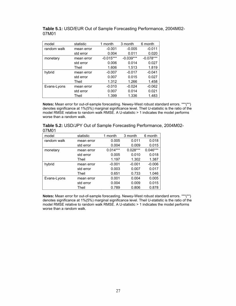
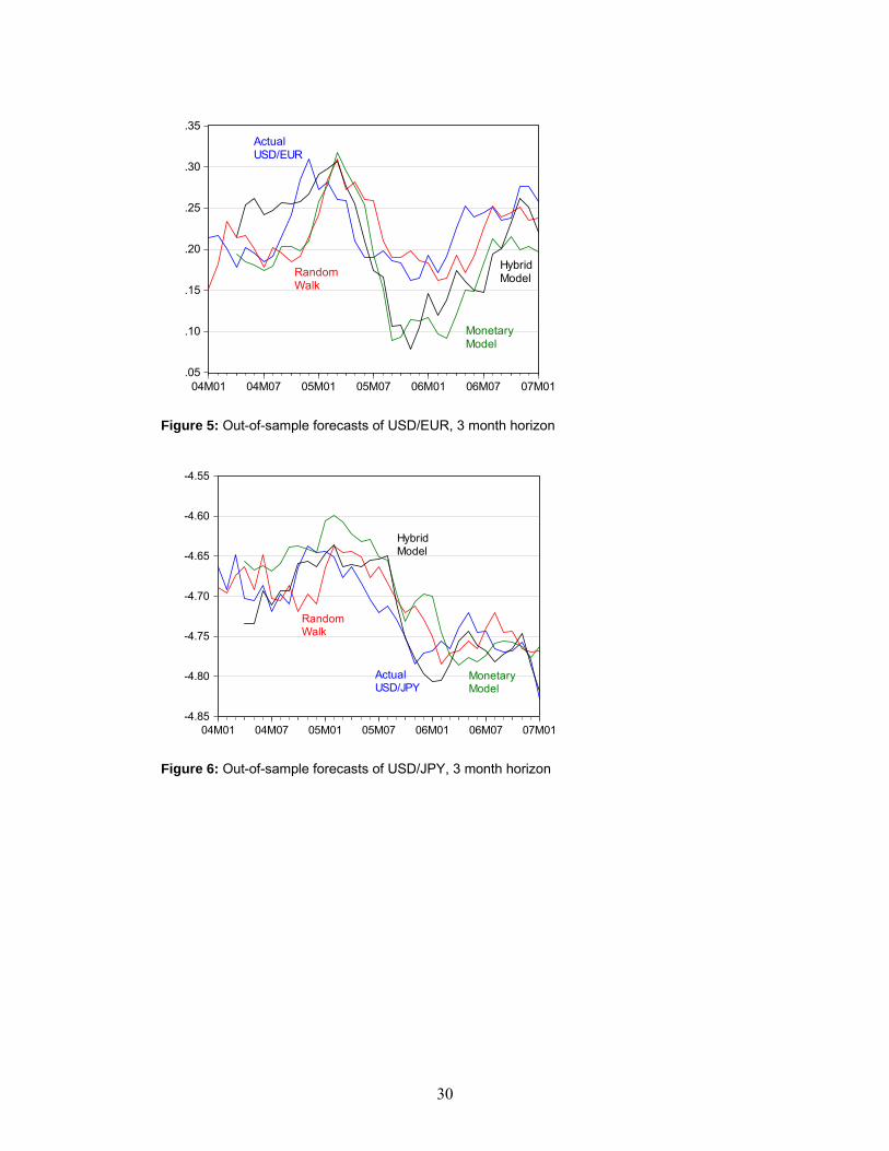
The results for the dollar/euro are reported in Table 5.1. The first two rows pertain to

the no-drift random walk forecast. The next two blocks of cells pertain to the

monetary model, and the hybrid model. The final block is the Evans-Lyons model,

which we include for purposes of comparison. Note that the Evans-Lyons model does

not incorporate a long run relationship incorporating cumulated order flow.18

Turning first to the dollar/euro exchange rate, notice that monetary model does very

badly relative to the random walk over this sample period. The ratio of the monetary

model to the random walk RMSE (the Theil U-statistic) is 1.61, 1.50 and 1.82 at the

1, 3 and 6 month horizons. In contrast, the mean error is smaller for the hybrid model

at all horizons, and Theil statistic (vis a vis the random walk) is much smaller: 1.31,

1.27, and 1.46. The relative performance of these forecasts (random walk, monetary,

hybrid) is shown in Figures 5 for the dollar/euro exchange rate.19

The results are slightly different in the case of the dollar/yen (see Table 6). There, by

the RMSE criterion, the hybrid model substantially outperforms the monetary model

at all horizons, and the Evans-Lyons specifications at 1 and 3 month horizons. Indeed,

the hybrid model even outperforms the random walk specification at the 1 and 3

month horizons.

8. Conclusion

We have laid out a simple and transparent framework in which non-stationary private

liquidity preference shocks give rise to instability in the demand for money and the 18 The particular specification we use conforms to columns [3] and [7] in Table 1. 19 The RMSE for the hybrid model is smaller than the random walk at the 3 and 6 month horizons if non-demeaned cumulative order flow data is used. Given the upward bias in the model-based RMSE versus the random walk RMSE (see Clark and West, 2007), this suggests an improvement vis à vis the random walk benchmark.

18

apparent failure of the monetary model of exchange rates. Cumulative order flow

tracks these shocks and provides the ‘missing link’ to augmenting the explanatory

power of conventional monetary models. We show that the hybrid model beats both

the monetary model and a random walk in a simple forecasting exercise. Berger et al.

(2006) concluded that while order flow plays a crucial role in high-frequency

exchange rate movements, its role in driving long-term fluctuations is much more

limited. We contend that this conclusion is premature.

In summary, we find substantial evidence to support our proposition that order flow is

an important variable in exchange rate determination, whose role can be rationalized

on the basis of a straightforward macroeconomic model. One of the appetizing

implications of the household optimizing problem as specified in equations (1) to (4)

is that consumption in country j also depends on the unit root parameter jtβ . This

means that the international consumption differential depends on H Ft tβ β− and

therefore on order flow from our interpretation. This may go some distance to explain

the international consumption correlations puzzle. However, we leave this to later

work.

19

Data Appendix

For the conventional macroeconomic variables, monthly frequency data were

downloaded from International Financial Statistics (accessed November 4, 2007).

End of month data used for exchange rates when used as a dependent variable.

Interest rates are monthly averages of daily data, and are overnight rates (Fed Funds

for the US, interbank rates for the euro area, and call money rate for Japan). In the

basic regressions, money is M2 (the ECB-defined M3 for Euro area), although

specifications using M1 were also estimated. Consumption is proxied by industrial

production, while inflation is 1 month log-differenced CPI in the basic regressions.

Specifications were also estimated using 3 month and 12 month log-differenced CPI

as a measure of inflation. Money, industrial production and CPIs are seasonally

adjusted.

Order flow was obtained from Electronic Broking Services (EBS). In order to make

the specifications consistent across currencies, the order flow data is converted to

dollar terms by dividing by the period-average exchange rate (for OFEURUSD) and

by putting a negative in front (for OFUSDJPY). Hence, the exchange rates are defined

(USD/EUR, USD/JPY) and order flow transformed so that the implied coefficient is

positive.

In some unreported regressions, the order flows are normalized by volume. Order

flow volume was also converted to dollar terms, in the same manner that order flow

was converted.

20

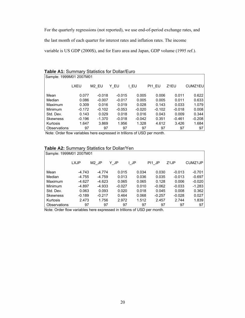
For the quarterly regressions (not reported), we use end-of-period exchange rates, and

the last month of each quarter for interest rates and inflation rates. The income

variable is US GDP (2000$), and for Euro area and Japan, GDP volume (1995 ref.).

Table A1: Summary Statistics for Dollar/Euro Sample: 1999M01 2007M01

LXEU M2_EU Y_EU I_EU PI1_EU Z1EU CUMZ1EU

Mean 0.077 -0.018 -0.015 0.005 0.006 0.011 0.622 Median 0.086 -0.007 -0.017 0.005 0.005 0.011 0.633 Maximum 0.309 0.016 0.019 0.028 0.143 0.033 1.079 Minimum -0.172 -0.102 -0.053 -0.020 -0.102 -0.018 0.008 Std. Dev. 0.143 0.029 0.018 0.016 0.043 0.009 0.344 Skewness -0.196 -1.370 -0.018 -0.042 0.351 -0.461 -0.208 Kurtosis 1.647 3.869 1.956 1.328 4.612 3.426 1.684 Observations 97 97 97 97 97 97 97

Note: Order flow variables here expressed in trillions of USD per month. Table A2: Summary Statistics for Dollar/Yen Sample: 1999M01 2007M01

LXJP M2_JP Y_JP I_JP PI1_JP Z1JP CUMZ1JP

Mean -4.743 -4.774 0.015 0.034 0.030 -0.013 -0.701 Median -4.755 -4.759 0.013 0.036 0.035 -0.013 -0.697 Maximum -4.627 -4.623 0.065 0.065 0.128 0.006 -0.020 Minimum -4.897 -4.933 -0.027 0.010 -0.062 -0.033 -1.283 Std. Dev. 0.063 0.093 0.020 0.018 0.045 0.008 0.362 Skewness -0.189 -0.217 0.464 0.068 -0.257 -0.028 0.027 Kurtosis 2.473 1.756 2.972 1.512 2.457 2.744 1.839 Observations 97 97 97 97 97 97 97

Note: Order flow variables here expressed in trillions of USD per month.

21

References

Alquist, Ron and Menzie Chinn (2008). “Conventional and Unconventional Approaches to Exchange Rate Modeling and Assessment,” International Journal of Finance and Economics 13, pp. 2-13.

Berger, David, Alain Chaboud, Sergei Chernenko, Edward Howorka, and Jonathan Wright (2006). “Order Flow and Exchange Rate Dynamics in Electronic Brokerage System Data,” Board of Governors of the Federal Reserve System, International Finance Discussion Papers No. 830.

Bjønnes, Geir H and Dagfinn Rime (2005), “Dealer Behavior and Trading Systems in the Foreign Exchange Market", Journal of Financial Economics, vol. 75, issue 3 (March), pp. 571-605.

Cheung, Yin-Wong, Menzie D. Chinn, and Antonio Garcia Pascual (2005), “What do we know about recent exchange rate models? In-sample fit and out-of-sample performance evaluated,” In: DeGrauwe, P. (Ed.), Exchange Rate Modelling: Where Do We Stand? MIT Press for CESIfo, Cambridge, MA, pp. 239-276 (a).

Cheung Yin-Wong, Menzie D. Chinn and Antonio Garcia Pascual (2005), “Empirical exchange rate models of the nineties: Are any fit to survive?” Journal of International Money and Finance 24, pp 1150-1175 (b). Cheung, Yin-Wong and Kon. S. Lai (1993), “Finite-Sample Sizes of Johansen's Likelihood Ratio Tests for Cointegration,” Oxford Bulletin of Economics and Statistics, 55(3), pp. 313-328. Clark, Todd E. and Kenneth D. West (2007), “Using Out-of-Sample Mean Squared Prediction Errors to Test the Martingale Difference Hypothesis,” Journal of Econometrics 138(1), pp. 291-311. Diebold, Francis X. and Roberto Mariano (1995), “Comparing Predictive Accuracy,” Journal of Business and Economic Statistics 13, pp. 253-265. Evans M. (2008), “Order Flows and The Exchange Rate Disconnect Puzzle”, mimeo, June. Evans M., and R. Lyons (2002), “Order flow and exchange rate dynamics”. Journal of Political Economy, (February), 110(1), pp. 170–180. Evans, M., and R. Lyons (2005), “Meese-Rogoff Redux: Micro-based Exchange Rate Forecasting”, American Economic Review Papers and Proceedings, pp. 405-414. Evans, M., and R. Lyons (2008), “How Is Macro News Transmitted to Exchange Rates?”, Journal of Financial Economics, Volume 88, Issue 1, pp 26-50.

22

Flood, Robert P. and Andrew K. Rose (1999), “Understanding Exchange Rate Volatility without the Contrivance of Macroeconomics”, The Economic Journal 109(459), Features. (Nov.), pp. F660-F672. Gourinchas, Pierre-Olivier and Helene Rey (2007), “International Financial Adjustment,” Journal of Political Economy 115(4), pp. 665-773. Hollifield, B., R. Miller, and P. Sandas, (2004), “Empirical Analysis of Limit Order Markets”, Review of Economic Studies, Volume 71(4), 1027 - 1063. Killeen, William, Richard K. Lyons and Michael Moore (2006), “Fixed versus Flexible: Lessons from EMS Order Flow”, Journal of International Money and Finance 25, pp. 551-579. Lee, C., and M. Ready, (1991), “Inferring Trade Direction from Intraday Data”, Journal of Finance, Volume 46(2), 733-46. Meese, Richard, and Kenneth Rogoff (1983), “Empirical Exchange Rate Models of the Seventies: Do They Fit Out of Sample?” Journal of International Economics 14, pp. 3-24. Moore, Michael J. and Roche, Maurice J. (2002), “Less of a Puzzle: a New Look at the Forward Forex Market.” Journal of International Economics 58 (December), pp. 387-411. Moore, Michael J. and Roche, Maurice J. (2005), “A neo-classical explanation of nominal exchange rate volatility” in Exchange Rate Economics: Where do we stand? edited by Paul de Grauwe, MIT Press. Moore, Michael J. and Roche, Maurice J. (2007), “Solving Exchange Rate Puzzles with neither Sticky Prices nor Trade Costs”, Mimeo, Queen’s University, Belfast, September. Moore, Michael J. and Roche, Maurice J. (2008) “Volatile and Persistent Real Exchange Rates with or without Sticky Prices”, Journal of Monetary Economics, Volume 55, Issue 2, pp 423-433. Parlour, Christine A., (1998) “Price Dynamics in Limit Order Markets”, Review of Financial Studies, Volume 11, Number 4, pp. 789-816. Stock, James, and Watson, Mark, 1993, “A Simple Estimator of Cointegrated Vectors in Higher Order Integrated Systems,” Econometrica 61: 783-820. Verdelhan, Adrien (2007), “A Habit-Based Explanation of the Exchange Rate Risk Premium.” Mimeo, Boston University, June. West, Kenneth D. (1996), “Asymptotic Inference about Predictive Ability” Econometrica 64, pp. 1067-1084

23

Table 1: Evans-Lyons specification, 1999M02-2007M01 coefficient [1] [2] [3] [4] [5] [6] [7] [8] USD/EUR USD/JPY constant 0.003 -0.012 -0.009 0.003 0.005 0.023 0.030 0.005 0.003 0.005 0.005 0.003 0.006 0.004 0.007 0.006 Int. diff. -0.410 -0.270 -0.405 -0.172 -0.186 -0.170 0.169 0.182 0.171 0.147 0.145 0.140 OF 1.179 1.080 1.799 1.807 0.333 0.333 0.301 0.312 Δ OF 0.392 1.114 0.258 0.156 adj.R sq. 0.05 0.16 0.17 0.06 0.01 0.34 0.35 0.24N 96 96 96 96 96 96 96 96

Notes: Top entry is the OLS regression coefficient while the bottom entry is the Newey-West robust standard error. Bold face denotes coefficients significant at the 10% marginal significance level. Int. Diff. is the money market interest differential, OF is order flow in trillions of USD.

24

Table 2: Johansen Cointegration Test Results, 1999M04-2007M01

[1] [2] [3] [4] [5] [6] Monetary Fundamentals Hybrid USD/EUR asy 1,1 3,1 1,1 3,1 3,1 4,2 fs 1,1 1,1 1,1 1,1 1,1 2,1 USD/JPY asy 2,2 2,1 1,1 4,2 2,1 1,1 fs 2,2 1,1 1,1 2,0 0,0 0,0

Notes: Implied number of cointegrating vectors using Trace, Maximal Eigenvalue statistics and 5% marginal significance level. “Asy” (“fs”) denotes number of cointegrating vectors using asymptotic (finite sample) critical values (Cheung and Lai, 1993). Columns [1] and [4] indicate a constant is allowed in the cointegrating equation and none in the VAR; columns [2] and [5] indicate a constant is allowed in the cointegrating equation and in the VAR; columns [3] and [6] indicate an intercept and trend is allowed in the cointegrating equation and a constant in the VAR. Bold italics denotes the trend specification with the lowest AIC for single cointegrating vector case. All results pertain to specifications allowing for 4 lags in the levels-VAR specification.

25

Table 3: USD/EUR Monetary/Order Flow Hybrid Exchange Rate Regression Results, 1999M04-2007M01 coefficient [1] [2] [3] [4] constant 0.001 -0.016 -0.005 -0.019 0.003 0.004 0.004 0.008 Δmoney t-1 -0.623 -1.265 -0.759 -1.210 0.451 0.424 0.446 0.440 Δincome t-1 -0.037 0.027 -0.043 0.140 0.344 0.334 0.314 0.342 Δint rate t-1 2.407 2.550 2.457 1.696 1.800 1.257 1.741 1.398 Δinfl rate t-1 -0.033 -0.022 -0.019 0.000 0.049 0.039 0.050 0.034 Δ ex rate t-1 0.156 0.220 0.065 0.194 0.090 0.072 0.111 0.071 ECT t-1 -0.057 -0.043 -0.053 0.012 0.038 0.030 0.038 0.028 money -3.928 -3.928 -3.928 -0.420 0.489 0.489 0.489 1.337 income 5.514 5.514 5.514 5.119 2.793 2.793 2.793 2.556 int rate -8.292 -8.292 -8.292 -2.954 3.020 3.020 3.020 2.609 infl rate 1.122 1.122 1.122 -0.314 1.019 1.019 1.019 1.027 OF t 1.492 0.316 0.306 0.109 OF t-1 0.612 0.301 Cum OF 1.564 0.308 time adj.R sq. 0.01 0.26 0.04 0.25N 94 94 94 94

Notes: Top entry is coefficient; robust standard error is bottom entry. Estimates from two step procedure. Coefficients on level variables (excluding order flow) are obtained using DOLS(2,2). Other coefficients are estimated from second stage error correction model. Bold face denotes significance at 10% msl. Variables in bold italics are in the cointegrating relationship.

26

Table 4: USD/JPY Monetary/Order Flow Hybrid Exchange Rate Regression Results, 1999M04-2007M01 coefficient [1] [2] [3] [4] constant -0.004 0.020 -0.008 0.019 0.003 0.004 0.004 0.005 Δmoneyt-1 0.267 0.359 0.196 0.440 0.493 0.369 0.509 0.360 Δincome t-1 0.553 0.421 0.531 0.309 0.233 0.197 0.227 0.201 Δint rate t-1 4.958 4.105 4.777 2.789 1.321 1.052 1.295 0.970 Δinfl rate t-1 -0.083 -0.076 -0.080 -0.059 0.035 0.029 0.035 0.029 Δ ex rate t-1 0.187 0.278 0.240 0.227 0.105 0.093 0.119 0.098 ECT t-1 -0.184 -0.155 -0.182 -0.040 0.043 0.042 0.044 0.045 money -0.143 -0.143 -0.143 0.271 0.123 0.123 0.123 1.873 income -1.947 -1.947 -1.947 -1.825 0.482 0.482 0.482 0.424 int rate -0.564 -0.564 -0.564 -0.099 0.291 0.291 0.291 1.309 infl rate 0.280 0.280 0.280 0.177 0.390 0.390 0.390 0.434 OF t 1.865 0.097 0.293 0.468 OF t-1 -0.310 0.298 Cum OF 1.893 0.321 time adj.R sq. 0.14 0.47 0.14 0.40N 94 94 94 94

Notes: Top entry is coefficient; robust standard error is bottom entry. Estimates from two step procedure. Coefficients on level variables (excluding order flow) are obtained using DOLS(2,2). Other coefficients are estimated from second stage error correction model. Bold face denotes significance at 10% msl. Variables in bold italics are in the cointegrating relationship.

27

Table 5.1: USD/EUR Out of Sample Forecasting Performance, 2004M02-07M01 model statistic 1 month 3 month 6 month random walk mean error -0.001 -0.005 -0.011 std error 0.004 0.011 0.020monetary mean error -0.015*** -0.039*** -0.078*** std error 0.006 0.014 0.027 Theil 1.606 1.513 1.819hybrid mean error -0.007 -0.017 -0.041 std error 0.007 0.015 0.027 Theil 1.312 1.266 1.458Evans-Lyons mean error -0.010 -0.024 -0.062 std error 0.007 0.014 0.021 Theil 1.399 1.336 1.483

Notes: Mean error for out-of-sample forecasting. Newey-West robust standard errors. ***(**) denotes significance at 1%(5%) marginal significance level. Theil U-statistic is the ratio of the model RMSE relative to random walk RMSE. A U-statistic > 1 indicates the model performs worse than a random walk. Table 5.2: USD/JPY Out of Sample Forecasting Performance, 2004M02-07M01 model statistic 1 month 3 month 6 month random walk mean error 0.005 0.011 0.018 std error 0.004 0.009 0.015monetary mean error 0.014*** 0.028*** 0.046*** std error 0.005 0.010 0.018 Theil 1.197 1.302 1.387hybrid mean error -0.001 -0.001 -0.006 std error 0.003 0.007 0.017 Theil 0.651 0.733 1.046Evans-Lyons mean error 0.001 0.004 0.005 std error 0.004 0.009 0.015 Theil 0.789 0.806 0.878

Notes: Mean error for out-of-sample forecasting. Newey-West robust standard errors. ***(**) denotes significance at 1%(5%) marginal significance level. Theil U-statistic is the ratio of the model RMSE relative to random walk RMSE. A U-statistic > 1 indicates the model performs worse than a random walk.

28

-20,000

-10,000

0

10,000

20,000

30,000

40,000

50,000

400,000

600,000

800,000

1,000,000

1,200,000

1,400,000

1,600,000

1,800,000

99 00 01 02 03 04 05 06

OFEURUSD VOLEURUSD

Figure 1: EUR/USD monthly order flow and order flow volume, in millions of euros.

-30,000

-20,000

-10,000

0

10,000

20,000

30,000

40,000

50,000

60,000

200,000

300,000

400,000

500,000

600,000

700,000

800,000

900,000

1,000,000

1,100,000

99 00 01 02 03 04 05 06

OFUSDJPY VOLUSDJPY

Figure 2: USD/JPY monthly order flow and order flow volume, in millions of dollars.

29

-.06

-.04

-.02

.00

.02

.04

.06

.08

-20,000 0 20,000 40,000

Z1EU

DLX

EU

Figure 3: First difference of log USD/EUR exchange rate and monthly net order flow in millions of USD (purchases of euros)

-.08

-.06

-.04

-.02

.00

.02

.04

.06

-40,000 -30,000 -20,000 -10,000 0 10,000

Z1JP

DLX

JP

Figure 4: First difference of log USD/JPY exchange rate and monthly net order flow in millions of USD (purchases of yen)

30

.05

.10

.15

.20

.25

.30

.35

04M01 04M07 05M01 05M07 06M01 06M07 07M01

ActualUSD/EUR

RandomWalk

MonetaryModel

HybridModel

Figure 5: Out-of-sample forecasts of USD/EUR, 3 month horizon

-4.85

-4.80

-4.75

-4.70

-4.65

-4.60

-4.55

04M01 04M07 05M01 05M07 06M01 06M07 07M01

ActualUSD/JPY

RandomWalk

MonetaryModel

HybridModel

Figure 6: Out-of-sample forecasts of USD/JPY, 3 month horizon