Embed Size (px)
Citation preview
Comput. Methods Appl. Mech. Engrg. 197 (2008) 3584–3592
Contents lists available at ScienceDirect
Comput. Methods Appl. Mech. Engrg.
journal homepage: www.elsevier .com/locate /cma
Probabilistic equivalence and stochastic model reduction in multiscale analysis
M. Arnst *, R. GhanemDepartment of Civil and Environmental Engineering, 210 KAP Hall, University of Southern California, Los Angeles, CA 90089, USA
a r t i c l e i n f o
Article history:Received 17 January 2008Received in revised form 9 March 2008Accepted 21 March 2008Available online 31 March 2008
Keywords:Multiscale modelingUncertainty quantificationUpscalingStochastic model reductionStochastic inverse analysisStochastic homogenization
0045-7825/$ - see front matter � 2008 Elsevier B.V. Adoi:10.1016/j.cma.2008.03.016
* Corresponding author. Tel.: +1 213 740 9165; faxE-mail addresses: [email protected] (M. Arnst), ghane
a b s t r a c t
This paper presents a probabilistic upscaling of mechanics models. A reduced-order probabilistic model isconstructed as a coarse-scale representation of a specified fine-scale model whose probabilistic structurecan be accurately determined. Equivalence of the fine- and coarse-scale representations is identified suchthat a reduction in the requisite degrees of freedom can be achieved while accuracy in certain quantitiesof interest is maintained. A significant stochastic model reduction can a priori be expected if a separationof spatial and temporal scales exists between the fine- and coarse-scale representations. The upscaling ofprobabilistic models is subsequently formulated as an optimization problem suitable for practical com-putations. An illustration in stochastic structural dynamics is provided to demonstrate the proposedframework.
� 2008 Elsevier B.V. All rights reserved.
1. Introduction
Advances in computing and sensing technologies and in numer-ical algorithms entertain the hope that prediction science couldsupersede computational science as the common rational contextfor scientific discovery and exploration. Concepts of model valida-tion and model-based certification shift the focus of the scientificendeavor from numerical analysis to scientific analysis, combiningthe tools of experimental physics, computational mechanics, andphysics. Advancing science along this new frontier faces two newchallenges. First, it is quickly recognized that most phenomena ofinterest, when resolved at the capacity of the new technologies,involve physical behaviors taking place at distinct scales, both spa-tial and temporal. Second, and while traditional computationalmechanics models yield deterministic predictions, physical realitypresents us with a range of possibilities that appear to be sampledat random every time nature is polled. This statistical multiscaleperspective seems to be critical to our ability to develop meaning-ful joint interpretations of model-based predictions and experi-mental observations. While statistical multiscale analysis owesits conceptual development to Gibbs [1], its tools and methods ofexploration have been continually reshaped to match technologicalresources and needs. One of the most significant ingredients in anymultiscale theory is the manner in which information is packagedas it is exchanged between scales. In a statistical context, this pack-aging is accomplished through a statistical description of the infor-mation, requiring an appropriate mathematical representation.
ll rights reserved.
: +1 213 740 [email protected] (R. Ghanem).
Thus, while representations using mean value or second-orderstatistics of the information being exchanged have been the essen-tial ingredient of many statistical multiscale paradigms, they pro-vide a limited albeit well-defined summary of this information.Complexity in alternative representations can quickly becometoo demanding. For example, representing information that exhib-its heterogeneity on the coarse scale requires recourse to stochasticprocesses, while situations where rare events dominate design cri-teria require recourse to stochastic models that are more faithfularound the tail of the associated probability measures. Recentprobabilistic parameterizations using the polynomial chaos theory[2] have paved the way for constructing non-gaussian stochasticprocesses that are well adapted to available information [3–6].
In the present paper we apply these stochastic representationsto propose a probabilistic model upscaling strategy, namely a pro-cedure for summarizing information available from a given fine-scale model in a different model constructed at a coarser scale suchthat both models provide equivalent predictions of some event ofinterest, usually defined in the sigma-algebra of the coarse-scalemodel. Although a mathematical description of the uncertainty inprobabilistic models may be often cast in an infinite-dimensionalcontext, it can be sufficiently characterized, in many applications,in a finite-dimensional setting using a finite number of randomvariables [7]. For example, probabilistic models are typically con-structed by modeling a finite number of uncertain fields of materialproperties and geometry by stochastic processes that are reducedthrough adapted techniques such as the Karhunen–Loeve decom-position [2]. The number of independent random variables fromwhich the uncertainty in a probabilistic model derives is referredto as the stochastic dimension of that model. This a functional
M. Arnst, R. Ghanem / Comput. Methods Appl. Mech. Engrg. 197 (2008) 3584–3592 3585
dimension of the probabilistic model and reflects the number ofindependent pieces of information on which the model could bemade to depend with sufficient accuracy. Models that necessitatefiner-scale fluctuations in the mathematical description of theirproperties will have a higher stochastic dimension, since a largernumber of random variables must be retained in the truncatedKarhunen–Loeve decomposition of the associated random fieldsto achieve a target fidelity.
The main objective of the present article is to show that a sto-chastic dimension reduction can be achieved in probabilistic modelupscaling through a judicious interpretation of equivalence affor-ded by the probabilistic setting. A significant stochastic modelreduction is a priori possible if a separation of spatial and temporalscales exists between the fine and coarse representations.
It should be noted that the multiscale framework is an essentialdifference of the proposed procedure compared to previous sto-chastic model reduction strategies. The latter most often act upona single probabilistic model defined at a single scale, and the maingoal of the reduction is usually to improve computational effi-ciency. Examples are the use of the Karhunen–Loeve decomposi-tion in e.g. [2,8,9] to deduce efficient discrete representations ofrandom fields of material properties and/or random response fieldsat a fixed scale.
The article is organized as follows: First, Sections 2 and 3 sum-marize the specific setting in which the methodology will be devel-oped together with a concise statement of the task to beundertaken by probabilistic model upscaling. Then, Section 4,which constitutes the core of this article, expounds on issues ofdimension reduction. Subsequently, Section 5 formulates theupscaling of probabilistic models as an optimization problem suit-able for practical computations, and Section 6 provides details toassist the reader in implementing the framework. Finally, Section7 provides an illustration in stochastic structural dynamics to dem-onstrate the proposed methodology.
2. Fine-scale probabilistic model
This section introduces a fine-scale probabilistic model, whichwill be used in the next section to summarize the task to be under-taken by probabilistic model upscaling techniques. The alreadywell-established methods for the construction of probabilisticmodels are not recalled, but the reader is referred to [10–14] forthe general theory of random variables and stochastic processes,to [2,15–22] for examples of the construction of probabilistic mod-els in computational mechanics, and to [2,7,23–26] for details onthe Karhunen–Loeve decomposition and the polynomial chaosexpansion, which will be used in the remaining of the article.
Let the fine-scale probabilistic model be a stochastic linearboundary value problem, with a stochastic operator and a deter-ministic input, of the following form:
KðnÞuðnÞ ¼ f a:s: ð1Þ
Let the stochastic operator depend on a finite number of stochasticprocesses representing uncertainty in such quantities as materialproperties and geometrical characteristics. Let each of the stochas-tic processes be discretized in terms of a finite number of real ran-dom variables via a truncated Karhunen–Loeve expansion. Thestochastic operator associated to the stochastic boundary valueproblem is thus assumed to explicitly depend on only a finite num-ber, say N, of real random variables. Let the latter be the compo-nents ðn1; . . . ; nNÞ of the vector n. Denoting the support of each ni
by Ci, the support of n is then obtained as C ¼ Ci � � � � � CN . We willassume, without loss of generality that C ¼ RN .
Let V be the space of functions that are sufficiently regular to de-scribe sample paths of the boundary value problem. The stochastic
operator n7!KðnÞ is thus a transformation of the basic random vari-ables from their sample space RN into the space LðV ;V 0Þ ofbounded linear transformations from V into its dual V 0. The stochas-tic output function n7!uðnÞ is viewed similarly as a transformationof the basic random variables: for a fixed input vector f in V 0, theprobabilistic model (1) defines a mapping n7!uðnÞ ¼KðnÞ�1f fromthe sample space RN into V. Let Pn be the probability measure in-duced by the random variables n on the measurable spaceðRN;BðRNÞÞ, where BðRNÞ is the Borel r-algebra over RN . The map-ping n7!KðnÞ implicitly transforms the probability distribution, Pn,of the basic random variables into the probability distribution of theoperator associated with the boundary value problem, and theprobabilistic model (1) subsequently propagates this distributionto the probability distribution of the output function.
The stochastic dimension of the fine-scale probabilistic model isdefined to be the number N of independent basic random variables.It is thought of as the number of independent sources of uncer-tainty in the operator associated to the boundary value problem.
3. Probabilistic model upscaling
The upscaling of a fine-scale probabilistic model is thought of asa three-step procedure. The probabilistic coarse-scale observablesare first identified. Following that, a model is selected to describethe evolution of these observables. This coarse scale model shouldpermit the prediction of the complete probabilistic information ofthe coarse state variables and will typically be parameterized by afinite set of stochastic processes. The identification of these pro-cesses is the subject of the third step, and it involves defining mea-sures of proximity between a quantity of interest observed throughthe fine-scale and the coarse scale models.
Let the coarse-scale model be a stochastic linear boundary valueproblem, with a stochastic operator and a deterministic input, ofthe form,
fKðgÞ~uðgÞ ¼ ~f a:s: ð2Þ
The tilde distinguishes the quantities appearing in model (2) fromthose in model (1). Let the stochastic operator g7!fKðgÞ dependon a finite number of unknown stochastic processes and a finitenumber of unknown random variables. Similarly to the previoussection, let these unknown stochastic processes and random vari-ables be identified with only a finite number, say this time n, ofindependent real random variables, which are gathered in the com-ponents ðg1; . . . ; gnÞ of the vector g. The random vector g is thoughtof as a vector collecting the sources of the uncertainty in the oper-ator associated to the boundary value problem. The third step in theupscaling procedure then amounts to the identification of the ran-dom vector g.
It should be noted that the selection of the coarse-scale modelmay be a significant challenge in situations where there is a varietyof models to choose from, or where no model is available. How-ever, these issues are not addressed in this paper.
4. Dimension reduction in probabilistic model upscaling
Upscaling techniques for deterministic models customarily[27–29] define the equality sought between the predictions ofthe fine-scale and the coarse-scale model by using both modelsto predict a coarse-scale quantity of interest. Were the dynamicalbehavior a structure under study, examples could be a deformationenergy for a particular coarse-scale deformation field, a low eigen-frequency, or a boundary impedance for a particular coarse-scaleboundary displacement. The coarse-scale model is then identifiedsuch that it predicts the same value for the quantity of interestas the fine-scale model.
3586 M. Arnst, R. Ghanem / Comput. Methods Appl. Mech. Engrg. 197 (2008) 3584–3592
Let the fine-scale probabilistic model (1) be used to predict acoarse-scale quantity of interest. The stochastic quantity of interestthus obtained, denoted by n7!wðnÞ, is thought of as a transforma-tion of the fine-scale basic random variables n. The mappingn7!wðnÞ propagates the probability distribution of the basic ran-dom variables, i.e. the probability measure Pn, to the probabilitydistribution of the quantity of interest. Let wðnÞ admit a probabilitydensity function f ð�Þ : W ! Rþ : w7!f ðwÞ. It is a mapping from thespace W of values of the quantity of interest into the positive realline. Let the coarse-scale probabilistic model (2) also be used topredict the quantity of interest to obtain the random variableg7! ~wðgÞ. Let ~wðgÞ admit a probability density function ~f ð�Þ :
W ! Rþ : w7!~f ðwÞ. The random vector g may then be identifiedsuch that the coarse-scale model predicts the same value for thequantity of interest as the fine-scale model.
Probability theory defines different senses in which two ran-dom variables can be considered to be the same, such as almostsure equality, equality in mean square and equality in distribution.The mathematical sense attributed to the equality sought betweenthe stochastic quantities of interest determines whether the con-structed coarse-scale model can be of lower stochastic dimensionthan the given fine-scale model, as explained next.
4.1. Almost sure equality of coarse-scale predictions
A first upscaling technique may consist in identifying a mappinggð�Þ : RN ! Rn that associates to the fine-scale basic random vari-ables n the coarse-scale basic random variables gðnÞ such that
wðnÞ ¼ ~wðgðnÞÞ a:s:; ð3Þ
or, equivalently, such that
Pn fn 2 RN : wðnÞ ¼ ~wðgðnÞÞg� �
¼ 1: ð4Þ
This upscaling technique associates to each realization of the fine-scale probabilistic model a corresponding realization of thecoarse-scale probabilistic model that predicts the same value forthe quantity of interest.
It is key to realize that what is really obtained by this upscalingtechnique is a coarse-scale probabilistic model that depends on thefine-scale basic random variablesfK gðnÞð Þ~u gðnÞð Þ ¼ ~f a:s: ð5Þ
In other words, the result of this upscaling technique is a con-structed coarse-scale model (5) that is defined on the same proba-bility triplet ðRN;BðRNÞ; PnÞ as the given fine-scale model (1).
Since the constructed coarse-scale model explicitly depends onthe fine-scale basic random variables, the stochastic dimension ofthis model is really N. Hence, there is, by construction, no dimen-sion reduction. For this reason, this upscaling technique will notbe elaborated further in the remaining of this article.
4.2. Equality in distribution of coarse-scale predictions
An alternative technique may consist in identifying a randomvector g such that
wðnÞ ¼ ~wðgÞ in distribution; ð6Þ
or, equivalently, such that
8w 2W : f ðwÞ ¼ ~f ðwÞ: ð7Þ
This upscaling technique associates to the fine-scale probabilisticmodel a corresponding coarse-scale probabilistic model that pre-dicts a statistically equal quantity of interest. Were the fine-scaleand the coarse-scale model both used to predict an ensemble ofrealizations of this quantity of interest, then both ensembles wouldhave the same statistical descriptors (as the number of realizations
tends to infinity), such as the same statistical moments and thesame quantiles.
The constructed coarse-scale probabilistic model is, this time, offormfKðgÞ~uðgÞ ¼ ~f a:s: ð8Þ
This coarse-scale model is defined on the probability tripletðRn;BðRnÞ; PgÞ, where the sample space Rn is the space of valuesof g, the events space BðRnÞ is the Borel r-algebra, and Pg is theprobability measure induced by g. Hence, the result of the upscalingprocedure is, this time, a constructed coarse-scale model (8) that isdefined on a different probability triplet than the given fine-scalemodel (1).
If the constructed coarse-scale model fulfills the equality in dis-tribution (6) while depending on a number n of basic coarse-scalerandom variables ðg1; . . . ; gnÞ that is smaller than the number N ofbasic fine-scale random variables ðn1; . . . ; nNÞ, then the upscalingprocedure has achieved a reduction of the stochastic dimension.
5. Probabilistic model upscaling as an optimization problem
The upscaling technique outlined in Section 4.2 is now reformu-lated as an optimization problem suitable for practical computa-tions. The objective (6) and (7) of achieving a perfect equalitybetween the probability density functions of the coarse-scalequantities of interest predicted by the fine-scale and the coarse-scale model is expected to be too strong for practical purposes. Itis natural to relax this objective by looking instead for a randomvector g that minimizes a distance between these probability den-sity functions
g ¼ arg ming
d f ðwÞ;~f ðwÞ� �
: ð9Þ
This functional infinite-dimensional optimization problem must bediscretized to make it suitable for a numerical solution. For this pur-pose, let g be approximated by a truncated Wiener polynomialchaos expansion of dimension n and order p
gðpÞ ¼Xp
a;jaj¼0
paHaðzÞ in mean square; ð10Þ
where the n components ðz1; . . . ; znÞ of the random vector z areindependent real Gaussian random variables with zero mean andunit standard deviation, a ¼ ða1; . . . ; anÞ 2 Nn is a multi-index, jaj ¼a1 þ � � � þ an, and HaðzÞ ¼ ha1 ðz1Þ � � � � � han ðznÞ, in which hak
ð�Þ isthe normalized Hermite polynomial of order ak. Let the coefficientsof this expansion be collected in the parameter set p ¼fpaj0 6 jaj 6 pg. Let ~f ð�jpÞ : W ! Rþ : w 7!~f ðwjpÞ denote the proba-bility density function of ~wðgðpÞÞ. The finite-dimensional optimiza-tion problem thus obtained reads
p ¼ arg minp
dðf ðwÞ;~f ðwjpÞÞ: ð11Þ
Several methods for defining distances between probability densityfunctions have already been developed within the theory of math-ematical statistics. Two such distances are presented in the remain-ing of this section, respectively based upon the generalized methodof moments and the divergence minimization method. The reader isreferred to [30–34] for standard texts on mathematical statistics,and to [35–39] for more details on the generalized method of mo-ments and the divergence minimization method.
5.1. Distance based upon the generalized method of moments
A first distance is defined as
dGMMðf ðwÞ;~f ðwjpÞÞ ¼ km� ~mðpÞk2 þ ckC � eCðpÞk2; ð12Þ
M. Arnst, R. Ghanem / Comput. Methods Appl. Mech. Engrg. 197 (2008) 3584–3592 3587
where c > 0 is a weighting factor chosen by the user, and in which
m ¼ EfwðnÞg;~mðpÞ ¼ Ef ~wðgðpÞÞg;C ¼ EfðwðnÞ �mÞ � ðwðnÞ �mÞg;eCðpÞ ¼ Efð ~wðgðpÞÞ � ~mðpÞÞ � ð ~wðgðpÞÞ � ~mðpÞÞg;
where Ef�g denotes the mathematical expectation. The distance (12)is the weighted sum of the least-squares distances between themean values and the covariance matrices of the stochastic quanti-ties of interest predicted by the fine-scale and the coarse-scalemodel. It is stressed that this distance is really a distance betweenstatistical descriptors of these stochastic quantities of interest. Itis not the mean-square norm of the difference of the random vari-ables n7!wðnÞ and gðpÞ7!wðgðpÞÞ, which cannot be meaningfully de-fined here since these random variables are not defined on the sameprobability triplet.
5.2. Distance based upon the divergence minimization method
A second distance is defined as
dDMMðf ðwÞ;~f ðwjpÞÞ ¼Z
Wf ðwÞ log
f ðwÞ~f ðwjpÞ
dw: ð13Þ
It is the relative entropy [33,40] between f ðwÞ and ~f ðwjpÞ, which isa well-known positively valued distance-like measure of the sepa-ration between probability density functions.
5.3. Comments on the choice of the distance functional
It is expected that different sets of parameters are optimal inthe sense of the optimization problem (11) for different choicesof the distance functional. The use of the distance (12) leads toan optimization problem that seeks to achieve a good fit only be-tween the first-order and the second-order moments of the quan-tities of interest. Hence, a potential disadvantage is that a coarse-scale model may be identified that predicts higher-order momentsfor the quantity of interest, which are arbitrarily different fromthose predicted by the fine-scale model. The use of the distance(13) leads in contrast to an optimization problem that seeks toachieve a good fit between all the moments, since probability den-sity functions aggregate information on all moments. However, apotential disadvantage is therefore that a good fit of the low-ordermoments (in practice often most important) may be sacrificed tofit higher-order moments. Finally, it is noted that a weightedsum of distances (12) and (13) may provide a distance that allowsto accurately capture the second-order moments, while givingsome importance to the tails of the distribution.
6. Implementation
Details are now provided to assist the reader in implementingthe framework. The finite element method is the natural methodfor the discretization of the spatial dimension associated to thefine-scale and the coarse-scale probabilistic models (1) and (2).The Monte Carlo simulation method is the appropriate methodfor the discretization of the random dimension, since the equalitiesin Eqs. (1) and (2) are written in the almost sure sense with respectto the random coordinate. Had these equations been written in theweak sense with respect to the random coordinate, the naturalmethodology for the discretization of the random dimensionwould have consisted in the Galerkin projection of the weak for-mulation then obtained onto a suitable approximating stochasticfunctional space [2]. Algorithm 1 lists step by step how the dis-tances (12) and (13) can be computed using the finite elementand Monte Carlo simulation methods.
Algorithm 1 (computation of either distance (12), or (13)).
� Step 1: initialization:
Choose, with reference to (10), n, p and p.Choose a number MC of Monte Carlo Samples.� Step 2: computation with the fine-scale probabilistic model:
First, simulate a set fns j 1 6 s 6MCg of independent andidentically distributed realizations of the fine-scale basicrandom variables n.Then, for each s 2 f1 6 s 6MCg, construct the fine-scalefinite element model associated to the realization ns toobtainKhðnsÞuhðnsÞ ¼ f h: ð14Þ
Finally, for each s 2 f1 6 s 6MCg, use the finite elementmodel (14) to predict the quantity of interest whðnsÞ asso-ciated to the realization ns.
� Step 3: computation with the coarse-scale probabilistic model:
First, simulate, with reference to (10), a setfzs j 1 6 s 6MCg of independent and identically distrib-uted realizations of the random vector z.Then, for each s 2 f1 6 s 6MCg, use (10) to compute therealization gsðpÞ of the coarse-scale basic random vari-ables associated with the realization zs.Subsequently, for each s 2 f1 6 s 6MCg, construct thecoarse-scale finite element model associated to the reali-zation gsðpÞ to obtain fKhðgsðpÞÞ~uhðgsðpÞÞ ¼ ~f h: ð15ÞFinally, for each s 2 f1 6 s 6MCg, use the finite elementmodel (15) to predict the quantity of interest ~whðgsðpÞÞassociated to the realization gsðpÞ.
� Step 4: numerical approximation of either distance (12), or (13)
Either approximate distance (12) bydGMM;h;MCðpÞ ¼ kmh;MC � ~mh;MCðpÞk2 þ ckCh;MC � eC h;MCðpÞk2;
ð16Þ
in which
mh;MC ¼ 1MC
XMC
s¼1
whðnsÞ;
~mh;MCðpÞ ¼ 1MC
XMC
s¼1
~whðgsðpÞÞ;
Ch;MC ¼ 1MC� 1
XMC
s¼1
ðwhðnsÞ �mh;MCÞ � ðwhðnsÞ �mh;MCÞ;
eC h;MCðpÞ ¼ 1MC� 1
XMC
s¼1
~whðgsðpÞÞ � ~mh;MCðpÞ� �
� ð ~whðgsðpÞÞ � ~mh;MCðpÞÞ:
Or approximate distance (13) by
dDMM;h;MCðpÞ ¼ 1MC
XMC
s¼1
logf h;MCðwhðnsÞÞ
~f h;MCðwhðnsÞjpÞ; ð17Þ
where f h;MCðwÞ and ~f h;MCðwjpÞ are approximations of theprobability density functions f ðwÞ and ~f ðwjpÞ estimatedfrom the samples fwhðnsÞ j 1 6 s 6MCg andf ~whðgsðpÞÞ j 1 6 s 6MCg, respectively.
Algorithm 1 requires in steps 2 and 3 the computation ofrealizations of random variables. Methods for the simulation ofrandom variables are surveyed in [41]. Step 4 requires the estima-tion of probability density functions from sets of samples. The ker-nel density estimation method is used in this work [42–44].
To numerically solve the optimization problem (11), we suggestapplying an exhaustive grid-search when the number of
3588 M. Arnst, R. Ghanem / Comput. Methods Appl. Mech. Engrg. 197 (2008) 3584–3592
parameters to be identified is three or less. Otherwise, consideringthat the distances to be minimized may have multiple local min-ima and that it may be difficult to accurately calculate gradientswith respect to the parameters, we suggest applying global-searchgradient-free optimization methods. The simulated annealingmethod [45,41,46] and the genetic optimization method [47,48]are natural choices. The latter is used in this work.
Finally, we suggest to apply a convergence analysis to deter-mine the optimal dimension n and order p in Eq. (10), i.e. to in-crease n and p until further increments no longer significantlyimprove the fit of the given fine-scale and the identified coarse-scale model. If this procedure leads to a coarse-scale model that fitsthe fine-scale model sufficiently well in the sense of the chosendistance functional while depending on a number n of basiccoarse-scale random variables that is smaller than the number Nof basic fine-scale random variables, then the upscaling procedurehas achieved a reduction of the stochastic dimension.
7. Illustration
7.1. Problem setting
This illustration concerns the dynamical behavior of a complexstructure, in particular of an assembly of plates joined together bythin layers of heterogeneous adhesive material. A fine-scale prob-abilistic model is built to predict the dynamical behavior in thelow-frequency and medium-frequency range. The objective is sub-sequently to identify a coarse-scale probabilistic model able to rep-resent the low-frequency dynamical behavior associated to thefirst structural eigenmode.
7.2. Fine-scale model
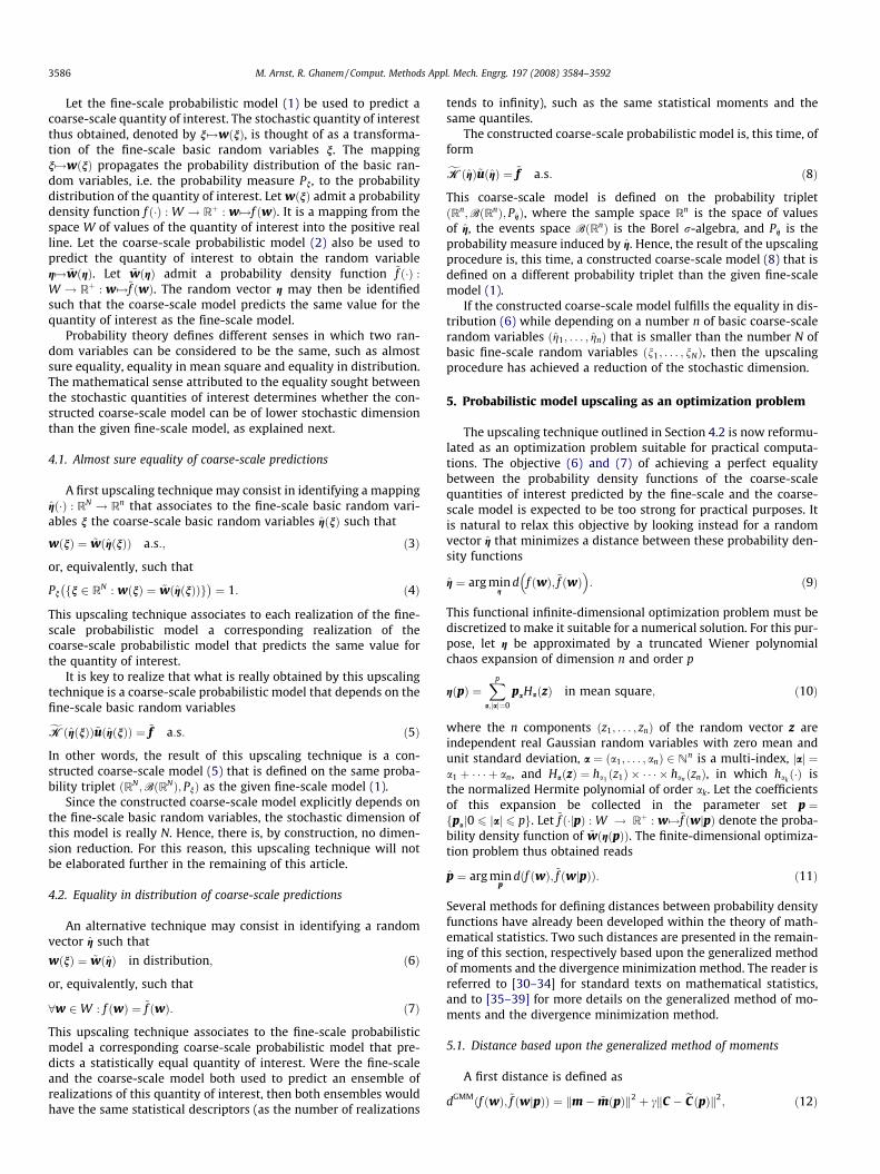
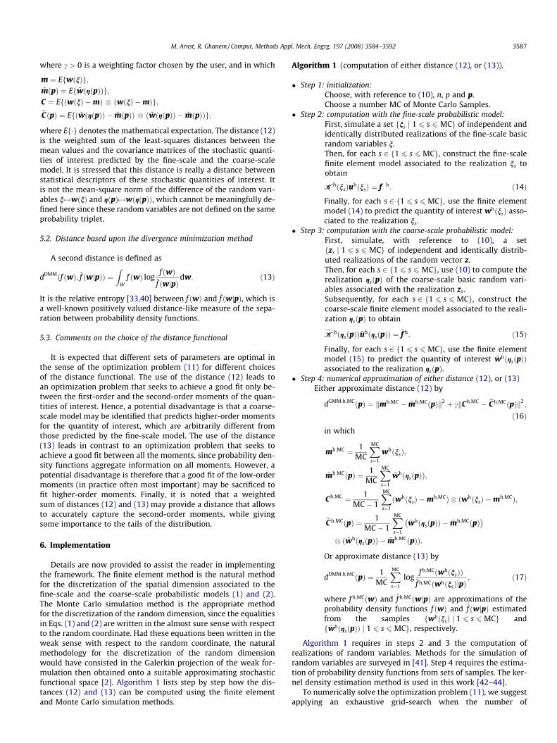
The fine-scale probabilistic model is a three-dimensionalcontinuum mechanics model. Fig. 1 shows the three-dimensionalfinite element mesh for the structure, made up of 34472 isopara-metric 8-noded brick elements. Fig. 2 shows the cross-section of
Fig. 1. Fine-scale model: the finite e
Fig. 2. Fine-scale model: cross-sect
the mesh. The structure is observed to be made up of 2 skin plates,3 longitudinal ribs, and 12 elongated L-shaped members.
A right-handed Cartesian reference frame ðx1; x2; x3Þ with origino is defined. Let the structure be circumscribed by the box-shapedregion
X ¼ � b2
m < x1 <b2;0 < x2 < ‘;� h
2m < x3 <
h2
� �; ð18Þ
in which w ¼ 9 m, h ¼ 2:94 m and ‘ ¼ 40 m are the width, heightand length of the structure. Let fxðkÞ j 1 6 k 6 10g denote a collec-tion of 10 equally-spaced points such that xðkÞ1 ¼ 0, xðkÞ2 ¼ k‘=10and xðkÞ3 ¼ h=2.
The material behavior of the skin plates, ribs and L-shapedstructural members is modeled using a linear, elastic, isotropicconstitutive equation with Young’s modulus 210E9 Pa, Poisson ra-tio 0.3 and mass density 7800 kg=m3. The plates and ribs are con-nected to the L-shaped members by means of 24 layers of adhesivematerial (two layers for each L-shaped member, joining that mem-ber to the adjacent skin plate and rib, respectively), modeled as aheterogeneous, linear, elastic, locally isotropic material with heter-ogeneous Young’s modulus field, homogeneous Poisson ratio 0.3and homogeneous mass density 7800 kg/m3.
The Young’s moduli fields of the layers of adhesive material aremodeled by independent stochastic processes, to be defined now.Let the stochastic process fgðx2Þ j 0 6 x2 6 ‘g with values in R bethe restriction to the closed interval ½0; ‘� of a sample-continuous,Gaussian, zero mean, unit variance, stationary random field withpower spectral density function k7!SðkÞ such that
SðkÞ ¼ Lp
DkLp
� ; ð19Þ
where Dð�Þ is the triangle function with compact support ½�1;1�such that
Dð0Þ ¼ 1; Dð�kÞ ¼ DðkÞ; DðkÞ ¼ 1� k for k 2 ½0;1�: ð20Þ
Let fEðx2Þ j 0 6 x2 6 ‘g be a lognormal process with values in Rþ0such that
lement mesh for the structure.
ion of the finite element mesh.
M. Arnst, R. Ghanem / Comput. Methods Appl. Mech. Engrg. 197 (2008) 3584–3592 3589
8x2 : Eðx2Þ ¼ E expffiffiffiffiffiffiffiffiffiffiffiffiffiffiffiffiffiffiffiffiffiffiffiffilogðd2 þ 1Þ
qgðx2Þ �
12
logðd2 þ 1Þ� �
a:s:
ð21Þ
The mean Young’s modulus is chosen equal to E ¼ 210E5 Pa, thedispersion level equal to d ¼ 2, and the spatial correlation lengthequal to L ¼ 20 m.
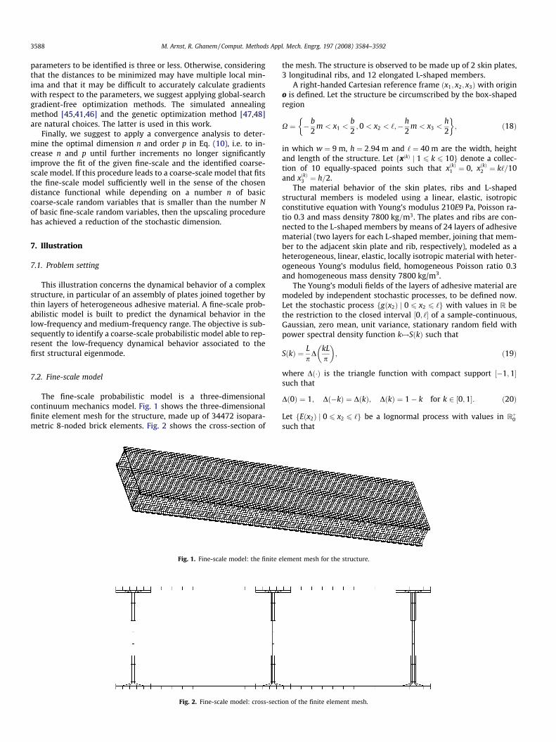
Fig. 3 shows the 10 largest eigenvalues of the covariance oper-ator of the stochastic process fgðx2Þ j 0 6 x2 6 ‘g, highlighting thatthis process can be discretized by truncating its Karhunen–Loeve
0 2 4 6 8 100
5
10
15
20
25
30
Index [–]
Eig
en v
alue
[–]
Fig. 3. Fine-scale model: 10 largest eigenvalues of the covariance operator of thestochastic process fgðx2Þj0 6 x2 6 ‘g.
0 1000 2000 30001.62
1.64
1.66
1.68
1.7
1.72
1.74
1.76
MC [–]
Freq
uenc
y [H
z]
0 1000 2000 30000
0.02
0.04
0.06
0.08
0.1
0.12
MC [–]
Freq
uenc
y [H
z]
Fig. 4. Fine-scale model: mean value and standard deviation of the first randomdynamical eigenfrequency as a function of the number MC of Monte Carlo samples.
decomposition after 3 terms, thereby preserving more than 99%of its dispersion. The 24 Young’s moduli fields are modeled by 24independent copies of the transformation (21) of the discretizedrandom field thus obtained. The fine-scale probabilistic structuralmodel is hence defined as a function of N ¼ 72 ¼ 24� 3 basic ran-dom variables.
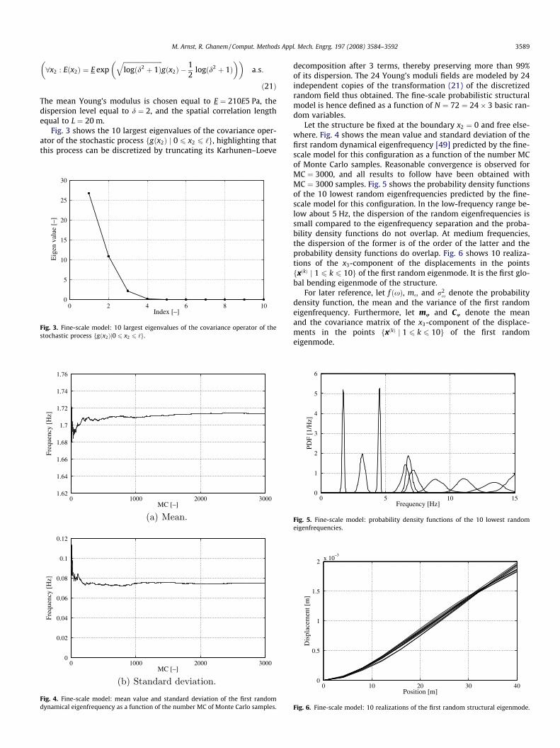
Let the structure be fixed at the boundary x2 ¼ 0 and free else-where. Fig. 4 shows the mean value and standard deviation of thefirst random dynamical eigenfrequency [49] predicted by the fine-scale model for this configuration as a function of the number MCof Monte Carlo samples. Reasonable convergence is observed forMC ¼ 3000, and all results to follow have been obtained withMC ¼ 3000 samples. Fig. 5 shows the probability density functionsof the 10 lowest random eigenfrequencies predicted by the fine-scale model for this configuration. In the low-frequency range be-low about 5 Hz, the dispersion of the random eigenfrequencies issmall compared to the eigenfrequency separation and the proba-bility density functions do not overlap. At medium frequencies,the dispersion of the former is of the order of the latter and theprobability density functions do overlap. Fig. 6 shows 10 realiza-tions of the x3-component of the displacements in the pointsfxðkÞ j 1 6 k 6 10g of the first random eigenmode. It is the first glo-bal bending eigenmode of the structure.
For later reference, let f ðxÞ, mx and r2x denote the probability
density function, the mean and the variance of the first randomeigenfrequency. Furthermore, let mu and Cu denote the meanand the covariance matrix of the x3-component of the displace-ments in the points fxðkÞ j 1 6 k 6 10g of the first randomeigenmode.
0 5 10 150
1
2
3
4
5
6
Frequency [Hz]
[1/H
z]
Fig. 5. Fine-scale model: probability density functions of the 10 lowest randomeigenfrequencies.
0 10 20 30 400
0.5
1
1.5
2x 10
–3
Position [m]
Dis
plac
emen
t [m
]
Fig. 6. Fine-scale model: 10 realizations of the first random structural eigenmode.
1.2 1.4 1.6 1.8 20
1
2
3
4
5
6
Frequency [Hz]
[1/H
z]
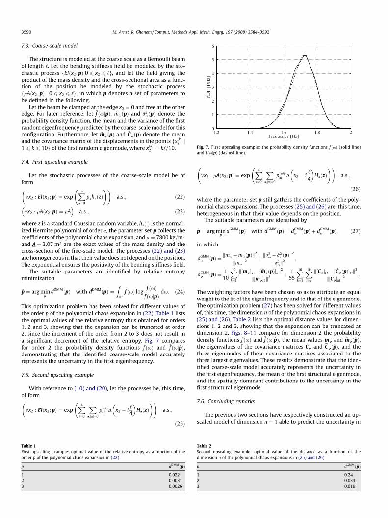
Fig. 7. First upscaling example: the probability density functions f ðxÞ (solid line)and ~f ðxjpÞ (dashed line).
3590 M. Arnst, R. Ghanem / Comput. Methods Appl. Mech. Engrg. 197 (2008) 3584–3592
7.3. Coarse-scale model
The structure is modeled at the coarse scale as a Bernoulli beamof length ‘. Let the bending stiffness field be modeled by the sto-chastic process fEIðx2; pÞj0 6 x2 6 ‘g, and let the field giving theproduct of the mass density and the cross-sectional area as a func-tion of the position be modeled by the stochastic processfqAðx2; pÞ j 0 6 x2 6 ‘g, in which p denotes a set of parameters tobe defined in the following.
Let the beam be clamped at the edge x2 ¼ 0 and free at the otheredge. For later reference, let ~f ðxjpÞ, ~mxðpÞ and ~r2
xðpÞ denote theprobability density function, the mean and the variance of the firstrandom eigenfrequency predicted by the coarse-scale model for thisconfiguration. Furthermore, let ~muðpÞ and eCuðpÞ denote the meanand the covariance matrix of the displacements in the points fxðkÞ2 j1 6 k 6 10g of the first random eigenmode, where xðkÞ2 ¼ k‘=10.
7.4. First upscaling example
Let the stochastic processes of the coarse-scale model be ofform
8x2 : EIðx2; pÞ ¼ expXp
a¼0
pahaðzÞ ! !
a:s:; ð22Þ
8x2 : qAðx2; pÞ ¼ qA� �
a:s:; ð23Þ
where z is a standard Gaussian random variable, hað�Þ is the normal-ized Hermite polynomial of order a, the parameter set p collects thecoefficients of the polynomial chaos expansion, and q ¼ 7800 kg=m3
and A ¼ 3:07 m2 are the exact values of the mass density and thecross-section of the fine-scale model. The processes (22) and (23)are homogeneous in that their value does not depend on the position.The exponential ensures the positivity of the bending stiffness field.
The suitable parameters are identified by relative entropyminimization
p ¼ arg minp
dDMMðpÞ with dDMMðpÞ ¼Z
Rþf ðxÞ log
f ðxÞ~f ðxjpÞ
dx: ð24Þ
This optimization problem has been solved for different values ofthe order p of the polynomial chaos expansion in (22). Table 1 liststhe optimal values of the relative entropy thus obtained for orders1, 2 and 3, showing that the expansion can be truncated at order2, since the increment of the order from 2 to 3 does not result ina significant decrement of the relative entropy. Fig. 7 comparesfor order 2 the probability density functions f ðxÞ and ~f ðxjpÞ,demonstrating that the identified coarse-scale model accuratelyrepresents the uncertainty in the first eigenfrequency.
7.5. Second upscaling example
With reference to (10) and (20), let the processes be, this time,of form
8x2 : EIðx2; pÞ ¼ expX4
ı¼0
X1
a;jaj¼0
pðEIÞai D x2 � i
‘
4
� HaðzÞ
! !a:s:;
ð25Þ
Table 1First upscaling example: optimal value of the relative entropy as a function of theorder p of the polynomial chaos expansion in (22)
p dDMMðpÞ
1 0.0222 0.00313 0.0026
8x2 : qAðx2; pÞ ¼ expX4
ı¼0
X1
a;jaj¼0
pðqAÞai D x2 � i
‘
4
� HaðzÞ
! !a:s:;
ð26Þ
where the parameter set p still gathers the coefficients of the poly-nomial chaos expansions. The processes (25) and (26) are, this time,heterogeneous in that their value depends on the position.
The suitable parameters are identified by
p ¼ arg minp
dGMMðpÞ with dGMMðpÞ ¼ dGMMx ðpÞ þ dGMM
u ðpÞ; ð27Þ
in which
dGMMx ðpÞ ¼ kmx � ~mxðpÞk2
kmxk2 þ kr2x � ~r2
xðpÞk2
kr2xk
2 ;
dGMMu ðpÞ ¼ 1
10
X10
k¼1
k½mu�k � ½ ~muðpÞ�kk2
k½mu�kk2 þ 1
55
X10
k¼1
X10
l¼k
k½Cu�kl � ½eCuðpÞ�klk2
k½Cu�klk2 :
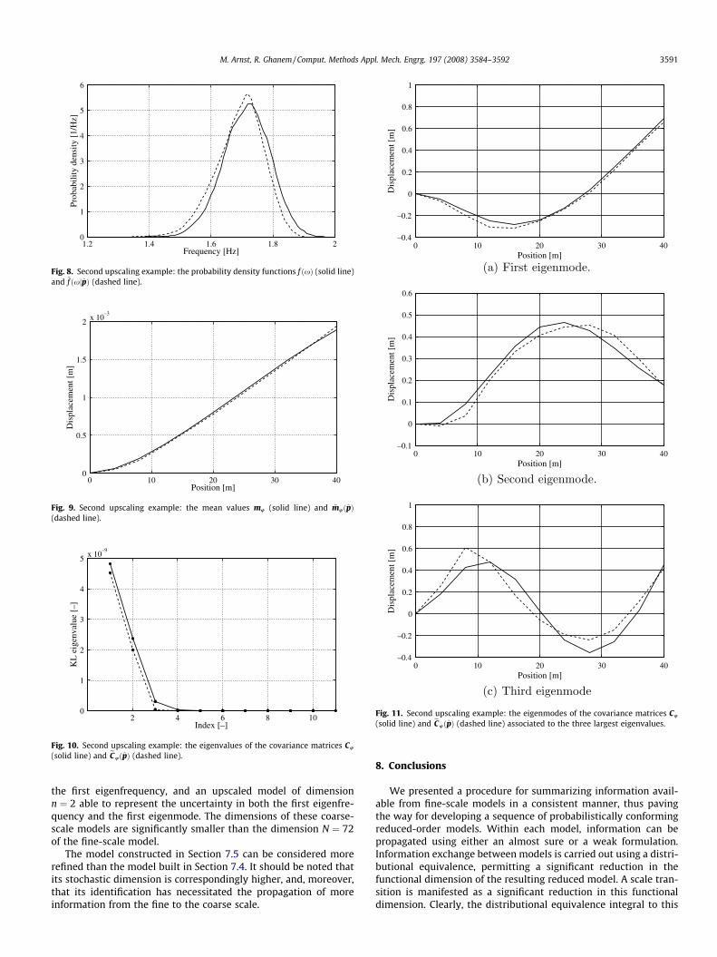
The weighting factors have been chosen so as to attribute an equalweight to the fit of the eigenfrequency and to that of the eigenmode.The optimization problem (27) has been solved for different valuesof, this time, the dimension n of the polynomial chaos expansions in(25) and (26). Table 2 lists the optimal distance values for dimen-sions 1, 2 and 3, showing that the expansion can be truncated atdimension 2. Figs. 8–11 compare for dimension 2 the probabilitydensity functions f ðxÞ and ~f ðxjpÞ, the mean values mu and ~muðpÞ,the eigenvalues of the covariance matrices Cu and eCuðpÞ, and thethree eigenmodes of these covariance matrices associated to thethree largest eigenvalues. These results demonstrate that the iden-tified coarse-scale model accurately represents the uncertainty inthe first eigenfrequency, the mean of the first structural eigenmode,and the spatially dominant contributions to the uncertainty in thefirst structural eigenmode.
7.6. Concluding remarks
The previous two sections have respectively constructed an up-scaled model of dimension n ¼ 1 able to predict the uncertainty in
Table 2Second upscaling example: optimal value of the distance as a function of thedimension n of the polynomial chaos expansions in (25) and (26)
n dGMMðpÞ
1 0.242 0.0333 0.019
1.2 1.4 1.6 1.8 20
1
2
3
4
5
6
Frequency [Hz]
Prob
abili
ty d
ensi
ty [
1/H
z]
Fig. 8. Second upscaling example: the probability density functions f ðxÞ (solid line)and ~f ðxjpÞ (dashed line).
0 10 20 30 400
0.5
1
1.5
2x 10
–3
Position [m]
Dis
plac
emen
t [m
]
Fig. 9. Second upscaling example: the mean values mu (solid line) and ~muðpÞ(dashed line).
2 4 6 8 100
1
2
3
4
5x 10
–9
Index [–]
KL
eig
enva
lue
[–]
Fig. 10. Second upscaling example: the eigenvalues of the covariance matrices Cu
(solid line) and eCuðpÞ (dashed line).
0 10 20 30 40–0.4
–0.2
0
0.2
0.4
0.6
0.8
1
Position [m]
Dis
plac
emen
t [m
]
0 10 20 30 40–0.1
0
0.1
0.2
0.3
0.4
0.5
0.6
Position [m]
Dis
plac
emen
t [m
]
0 10 20 30 40–0.4
–0.2
0
0.2
0.4
0.6
0.8
1
Position [m]
Dis
plac
emen
t [m
]
Fig. 11. Second upscaling example: the eigenmodes of the covariance matrices Cu
(solid line) and eCuðpÞ (dashed line) associated to the three largest eigenvalues.
M. Arnst, R. Ghanem / Comput. Methods Appl. Mech. Engrg. 197 (2008) 3584–3592 3591
the first eigenfrequency, and an upscaled model of dimensionn ¼ 2 able to represent the uncertainty in both the first eigenfre-quency and the first eigenmode. The dimensions of these coarse-scale models are significantly smaller than the dimension N ¼ 72of the fine-scale model.
The model constructed in Section 7.5 can be considered morerefined than the model built in Section 7.4. It should be noted thatits stochastic dimension is correspondingly higher, and, moreover,that its identification has necessitated the propagation of moreinformation from the fine to the coarse scale.
8. Conclusions
We presented a procedure for summarizing information avail-able from fine-scale models in a consistent manner, thus pavingthe way for developing a sequence of probabilistically conformingreduced-order models. Within each model, information can bepropagated using either an almost sure or a weak formulation.Information exchange between models is carried out using a distri-butional equivalence, permitting a significant reduction in thefunctional dimension of the resulting reduced model. A scale tran-sition is manifested as a significant reduction in this functionaldimension. Clearly, the distributional equivalence integral to this
3592 M. Arnst, R. Ghanem / Comput. Methods Appl. Mech. Engrg. 197 (2008) 3584–3592
upscaling procedure is adapted to specific quantities of interest,and it can be expected that the probabilistic scatter in the upscaledmodel will increase for all other predicted quantities.
Acknowledgements
This work was supported by NSF, Sandia National Laboratories,and a MURI administered by AFOSR on Health Monitoring andMaterials Damage Prognosis for Metallic Aerospace Propulsionand Structural Systems.
References
[1] W. Gibbs, On the equilibrium of heterogeneous substances. Trans. ConnecticutAcademy III, 1875–1878.
[2] R. Ghanem, P. Spanos, Stochastic Finite Elements: A Spectral Approach,Springer, 1991.
[3] C. Soize, A comprehensive overview of non-parametric probabilistic approachof random uncertainties for predictive models in structural dynamics, J. SoundVib. 288 (2005) 623–652.
[4] C. Desceliers, R. Ghanem, C. Soize, Maximum likelihood estimation ofstochastic chaos representations from experimental data, Int. J. Numer.Methods Engrg. 66 (2006) 978–1001.
[5] R.G. Ghanem, A. Doostan, On the construction and analysis of stochasticmodels: characterization and propagation of the errors associated with limiteddata, J. Comput. Phys. 217 (2006) 63–81.
[6] S. Das, R. Ghanem, J. Spall, Asymptotic sampling distribution for polynomialchaos representation of data: a maximum entropy and Fisher informationapproach, SIAM J. Scient. Comput., in press.
[7] C. Soize, R. Ghanem, Physical systems with random uncertainties: chaosrepresentations with arbitrary probability measure, SIAM J. Scient. Comput. 26(2004) 395–410.
[8] B. Ganapathysubramanian, N. Zabaras, Modeling diffusion in randomheterogeneous media: data-driven models, stochastic collocation and thevariational multiscale method, J. Comput. Phys. 226 (2007) 326–353.
[9] A. Doostan, R.G. Ghanem, J. Red-Horse, Stochastic model reduction for chaosrepresentations, Comput. Methods Appl. Mech. Engrg. 196 (2007) 3951–3966.
[10] Y.K. Lin, G.Q. Cai, Probabilistic Structural Dynamics, McGraw-Hill, 1995.[11] C. Soize, The Fokker–Planck Equation for Stochastic Dynamical Systems and Its
Explicit Steady State Solutions, World Scientific Publishing Company, 1994.[12] P. Krée, C. Soize, Mathematics of Random Phenomena: Random Vibrations of
Mechanical Structures, D. Reidel Publishing Company, 1986.[13] H. Cramér, M.R. Leadbetter, Stationary and Related Stochastic Processes:
Sample Function Properties and Their Applications, Dover Publications, 2004.[14] R.M. Dudley, Real Analysis and Probability, Cambridge University Press, 2002.[15] R.A. Ibrahim, Structural dynamics with parameter uncertainties, ASME Appl.
Mech. Rev. 40 (1987) 309–328.[16] C.S. Manohar, R.A. Ibrahim, Progress in structural dynamics with stochastic
parameter variations 1987–1998, ASME Appl. Mech. Rev. 52 (1999) 177–197.[17] G.I. Schueller, L.A. Bergman, C.G. Bucher, G. Dasgupta, G. Deotdatis, R.G. Ghanem,
M. Grigoriu, M. Hoshiya, E.A. Johnson, N.A. Naess, H.J. Pradlwarter, M. Shinozuka,K. Sobszyck, P.D. Spanos, B.F. Spencer, A. Sutoh, T. Takada, W.V. Wedig, S.F.Wojtkiewicz, I. Yoshida, B.A. Zeldin, R. Zhang, A state-of-the-art report oncomputational stochastic mechanics, Probab. Engrg. Mech. 12 (1997) 197–321.
[18] G.I. Schueller, Computational stochastic mechanics – recent advances,Comput. Struct. 79 (2001) 2225–2234.
[19] C. Soize, A non-parametric model of random uncertainties for reduced matrixmodels in structural dynamics, Probab. Engrg. Mech. 15 (2000) 277–294.
[20] C. Soize, Maximum entropy approach for modeling random uncertainties intransient elastodynamics, J. Acoust. Soc. Am. 109 (2001) 1979–1996.
[21] C. Soize, Non-Gaussian positive-definite matrix-valued random fields forelliptic stochastic partial differential operators, Comput. Methods Appl. Mech.Engrg. 195 (2006) 26–64.
[22] V.A.B. Narayanan, N. Zabaras, Variational multiscale stabilized FEMformulations for transport equations: stochastic advection–diffusion andincompressible stochastic Navier–Stokes equations, J. Comput. Phys. 202(2005) 94–133.
[23] R.H. Cameron, W.T. Martin, The orthogonal development of nonlinearfunctionals in series of Fourier–Hermite functionals, Ann. Math. 48 (1947)385–392.
[24] D. Xiu, G.E. Karniadakis, The Wiener–Askey polynomial chaos for stochasticdifferential equations, SIAM J. Scient. Comput. 24 (2002) 619–644.
[25] J. Mercer, Functions of positive and negative type and their connectionwith the theory of integral equations, Philos. Trans. Roy. Soc. A 209 (1909)415–446.
[26] N. Wiener, The homogeneous chaos, Am. J. Math. 60 (1938) 897–936.[27] J.H. Cushman, L.S. Bennethum, B.X. Hu, A primer on upscaling tools for porous
media, Adv. Water Resour. 25 (2002) 1043–1067.[28] C.L. Farmer, Upscaling: a review, Int. J. Numer. Methods Fluids 40 (2002) 63–
78.[29] W.K. Liu, E.G. Karpov, H.S. Park, Nano Mechanics and Materials: Theory,
Multiscale Methods and Applications, Wiley, 2006.[30] H. Cramér, Mathematical Methods of Statistics, Princeton University Press,
1946.[31] A. O’Hagan, J. Forster, Kendall’s Advanced Theory of Statistics, vol. 2B: Bayesian
Inference, Arnold Hodder, 2004.[32] A. Stuart, K. Ord, S. Arnold, Kendall’s Advanced Theory of Statistics, vol. 2A:
Classical Inference and the Linear Model, Arnold Hodder, 1999.[33] S. Kullback, Information Theory and Statistics, Dover Publications, 1968.[34] A. Tarantola, Inverse Problem Theory and Methods for Model Parameter
Estimation, SIAM, 2005.[35] L.P. Hansen, Large sample properties of generalized method of moments
estimators, Econometrica 50 (1982) 1029–1054.[36] W. Newey, D. McFadden, Large sample estimation and hypothesis testing, in:
R. Engle, D. McFadden (Eds.), Handbook of Econometrics IV, Elsevier, 1994, pp.2113–2247.
[37] A. Basu, B.G. Lindsay, Minimum disparity estimation for continuous models:efficiency, distributions and robustness, Annals of the Institute of StatisticalMathematics 46 (1994) 683–705.
[38] R. Beran, Minimum Hellinger distance estimates for parametric models, Ann.Statist. 5 (1977) 445–463.
[39] A. Keziou, Utilisation des divergences entre mesures en statistiqueinférentielle, PhD thesis, Université Paris 6, France, 2003.
[40] I. Csiszár, Information type measures of difference of probabilitydistributions and indirect observations, Stud. Scient. Math. Hungarica 2(1967) 299–318.
[41] C.P. Robert, G. Casella, Monte Carlo Statistical Methods, Springer, 2005.[42] E. Parzen, On estimation of probability density function and mode, Ann. Math.
Stat. 33 (1962) 1065–1076.[43] M. Rosenblatt, Remarks on some nonparametric estimates of a density
function, Ann. Math. Stat. 27 (1956) 832–837.[44] D.W. Scott, Multivariate Density Estimation: Theory, Practice, and
Visualization, Wiley-Interscience, 1992.[45] S. Kirkpatrick, C.D. Gelatt, M.P. Vecchi, Optimization by simulated annealing,
Science 220 (1983) 671–680.[46] N. Metropolis, A.W. Rosenbluth, M.N. Rosenbluth, A.H. Teller, E. Teller,
Equations of state calculations by fast computing machines, J. Chem. Phys.21 (1953) 1087–1092.
[47] D.E. Goldberg, Genetic Algorithms in Search, Optimization and MachineLearning, Addison-Wesley Professional, 1989.
[48] D.B. Fogel, Evolutionary Computation: Towards a New Philosophy of MachineIntelligence, IEEE Computer Society Press, 1995.
[49] M. Géradin, D. Rixen, Mechanical Vibrations: Theory and Applications toStructural Dynamics, Wiley, 1997.