Probabilistic Performance Models of Solar Plants 8pp

7/28/2019 Probabilistic Performance Models of Solar Plants 8pp

http://slidepdf.com/reader/full/probabilistic-performance-models-of-solar-plants-8pp 1/8

Clifford K. Ho

Gregory J. Kolb

Department of Solar Technologies,

Sandia National Laboratories,

P.O. Box 5800,

Albuquerque, NM 87185-1127

e-mail: [email protected]

Incorporating Uncertainty intoProbabilistic PerformanceModels of Concentrating SolarPower Plants

A method for applying probabilistic models to concentrating solar-thermal power plantsis described in this paper. The benefits of using probabilistic models include quantifica-tion of uncertainties inherent in the system and characterization of their impact on system

performance and economics. Sensitivity studies using stepwise regression analysis canidentify and rank the most important parameters and processes as a means to prioritize

future research and activities. The probabilistic method begins with the identification of uncertain variables and the assignment of appropriate distributions for those variables.Those parameters are then sampled using a stratified method (Latin hypercube sampling)to ensure complete and representative sampling from each distribution. Models of per-

formance, reliability, and cost are then simulated multiple times using the sampled set of parameters. The results yield a cumulative distribution function that can be used toquantify the probability of exceeding (or being less than) a particular value. Two ex-amples, a simple cost model and a more detailed performance model of a hypothetical

100-MW e power tower, are provided to illustrate the methods.

DOI: 10.1115/1.4001468

1 Introduction

Modeling the performance and economics of solar power plantsbased on technologies such as power towers and parabolic troughshas evolved over several decades. Yet nearly all of the modelingperformed previously implement deterministic evaluations of thesystem or component performance. Input parameters are typicallyentered as specific values rather than distributions of values thathonor the inherent uncertainty in many of the system features andprocesses. As a result, the confidence of the deterministic resultand uncertainty associated with the results are unknown.

This paper presents a probabilistic method to yield uncertaintyanalyses that can quantify the impact of system uncertainties onthe simulated performance metrics. The confidence and likelihoodof the simulated metric e.g., levelized energy cost being aboveor below a particular value or within a given range can be readilyassessed and presented using these probabilistic methods. In ad-dition, sensitivity analyses can be used with probabilistic analysesto rank and quantify the most important components, features,and/or processes that impact the simulated performance. This in-formation can be used to guide and prioritize future research andcharacterization activities that are truly important to the relevantperformance metrics.

Probabilistic methods are used widely in many fields includingrisk assessments and waste management, and they are required bythe Nuclear Regulatory Commission for performance assessments

of nuclear waste repositories 1 . Becker and Klimas 2 imple-mented a probabilistic method for simulating a hypothetical100-MWe power tower using the levelized energy cost as a metric.This work extends the work of Becker and Klimas 2 and inves-tigates additional examples and performance metrics e.g., net an-nual energy production . Direct costs are also updated to reflectinflation factors from 1990 to 2008.

2 Modeling Approaches

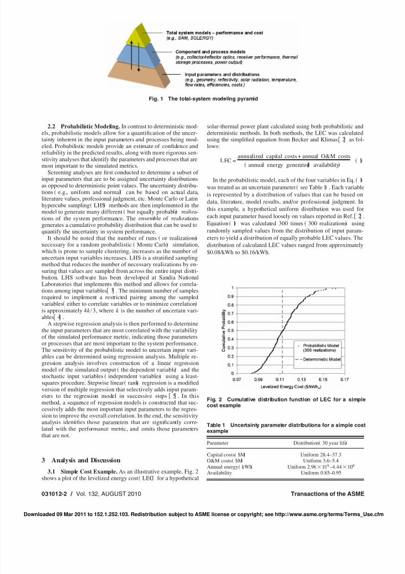
Models and codes used to model solar-thermal power plants can

be grouped according to a total-system modeling pyramid, which

describes a natural hierarchy for modeling complex systems Fig.

1 . At the top, total-system models are used to evaluate overall

performance metrics such as levelized energy cost or power out-

put. These total-system models rely on input from more detailed

process models that provide information regarding the perfor-

mance of individual components within the total system. The

process models require input parameters and distributions foruncertainty and sensitivity analyses that are acquired through

various means such as testing, literature, surveys, and/or profes-

sional judgment. This modeling pyramid is often used as the

framework for modeling complex systems because it provides a

logical flow and organization of the information and modeling

activities.

In addition to passing information up from the detailed process

models and parameters, the framework calls for information being

passed down from the top to assist in prioritizing modeling and

characterization efforts in areas that have been shown in the mod-

els to significantly impact the relevant cost and performance met-

rics.

2.1 Deterministic Modeling. Deterministic models use single

or central value estimates for each input parameter. For each

state or scenario of the physical system that is modeled, a unique

set of input parameters and boundary conditions is applied. There-

fore, deterministic models yield a single result for each scenario

modeled, and the uncertainty associated with the result is not

quantified. Sensitivity analyses can be performed parametrically

by selectively varying input parameter values to determine the

potential impact on the simulated metric. However, this process

can be arduous with more than a few parameters, and sensitivities

can be confounded by interactions among parameters that have

dependencies on one another.

Contributed by the Solar Energy Division of ASME for publication in the JOUR-

NAL OF SOLAR ENERGY ENGINEERING. Manuscript received August 21, 2009; finalmanuscript received December 13, 2009; published online June 21, 2010. Assoc.Editor: Manuel Romero Alvarez.

Journal of Solar Energy Engineering AUGUST 2010, Vol. 132 / 031012-1Copyright © 2010 by ASME

Downloaded 09 Mar 2011 to 152.1.252.103. Redistribution subject to ASME license or copyright; see http://www.asme.org/terms/Terms_Use.cfm



2.2 Probabilistic Modeling. In contrast to deterministic mod-els, probabilistic models allow for a quantification of the uncer-tainty inherent in the input parameters and processes being mod-eled. Probabilistic models provide an estimate of confidence andreliability in the predicted results, along with more rigorous sen-sitivity analyses that identify the parameters and processes that aremost important to the simulated metrics.

Screening analyses are first conducted to determine a subset of input parameters that are to be assigned uncertainty distributionsas opposed to deterministic point values. The uncertainty distribu-tions e.g., uniform and normal can be based on actual data,

literature values, professional judgment, etc. Monte Carlo or Latinhypercube sampling LHS methods are then implemented in themodel to generate many different but equally probable realiza-tions of the system performance. The ensemble of realizationsgenerates a cumulative probability distribution that can be used toquantify the uncertainty in system performance.

It should be noted that the number of runs or realizationsnecessary for a random probabilistic Monte Carlo simulation,which is prone to sample clustering, increases as the number of uncertain input variables increases. LHS is a stratified samplingmethod that reduces the number of necessary realizations by en-suring that values are sampled from across the entire input distri-bution. LHS software has been developed at Sandia NationalLaboratories that implements this method and allows for correla-tions among input variables 3 . The minimum number of samplesrequired to implement a restricted pairing among the sampledvariables either to correlate variables or to minimize correlationis approximately 4k /3, where k is the number of uncertain vari-ables 4 .

A stepwise regression analysis is then performed to determinethe input parameters that are most correlated with the variabilityof the simulated performance metric, indicating those parametersor processes that are most important to the system performance.The sensitivity of the probabilistic model to uncertain input vari-ables can be determined using regression analysis. Multiple re-gression analysis involves construction of a linear regressionmodel of the simulated output the dependent variable and thestochastic input variables independent variables using a least-squares procedure. Stepwise linear rank regression is a modifiedversion of multiple regression that selectively adds input param-eters to the regression model in successive steps 5 . In this

method, a sequence of regression models is constructed that suc-cessively adds the most important input parameters to the regres-sion to improve the overall correlation. In the end, the sensitivityanalysis identifies those parameters that are significantly corre-lated with the performance metric, and omits those parametersthat are not.

3 Analysis and Discussion

3.1 Simple Cost Example. As an illustrative example, Fig. 2shows a plot of the levelized energy cost LEC for a hypothetical

solar-thermal power plant calculated using both probabilistic anddeterministic methods. In both methods, the LEC was calculatedusing the simplified equation from Becker and Klimas 2 as fol-lows:

LEC =annualized capital costs + annual O&M costs

annual energy generated availability 1

In the probabilistic model, each of the four variables in Eq. 1

was treated as an uncertain parameter see Table 1 . Each variable

is represented by a distribution of values that can be based on

data, literature, model results, and/or professional judgment. Inthis example, a hypothetical uniform distribution was used for

each input parameter based loosely on values reported in Ref. 2 .

Equation 1 was calculated 300 times 300 realizations using

randomly sampled values from the distribution of input param-

eters to yield a distribution of equally probable LEC values. The

distribution of calculated LEC values ranged from approximately

$0.08/kWh to $0.16/kWh.

Fig. 2 Cumulative distribution function of LEC for a simplecost example

Fig. 1 The total-system modeling pyramid

Table 1 Uncertainty parameter distributions for a simple costexample

Parameter Distribution 30 year life

Capital costs $M Uniform 28.4–37.3O&M costs $M Uniform 3.6–5.4Annual energy kWh Uniform 2.96ϫ108 –4.44ϫ108

Availability Uniform 0.85–0.95

031012-2 / Vol. 132, AUGUST 2010 Transactions of the ASME




Figure 2 shows these results as a cumulative distribution func-tion CDF or cumulative probability. This plot can be used topredict the probability of the LEC being less or more than aparticular value, or between two values. For example, in this hy-pothetical example, there is approximately a 95% probability thatthe LEC will be less than ϳ$0.14 /kWhe and a 5% probability thatthe LEC will be greater than ϳ$0.14 /kWhe. There is approxi-

mately a 0.9−0.2=0.7 70% probability that the LEC will bebetween $0.10 /kWhe and $0.14 /kWhe.

The deterministic model, using average or “central” values forthe uncertain input parameters, predicts a LEC of just over$0.11/kWhe, which happens to be the median 50th percentile of the probabilistic model. This single value does not provide anyindication of the amount of uncertainty in the output e.g., thatthere is a 50% probability that the LEC will be greater than$0.11/kWhe in this hypothetical example . Also, the deterministicLEC value may shift left or right in Fig. 2 depending on the natureof the distributions used for the input parameters e.g., uniform,normal, and log-normal . For example, if most of the input distri-butions were log-normally distributed, the deterministic LECvalue may fall in the 20th to 30th percentile instead of the 50thpercentile.

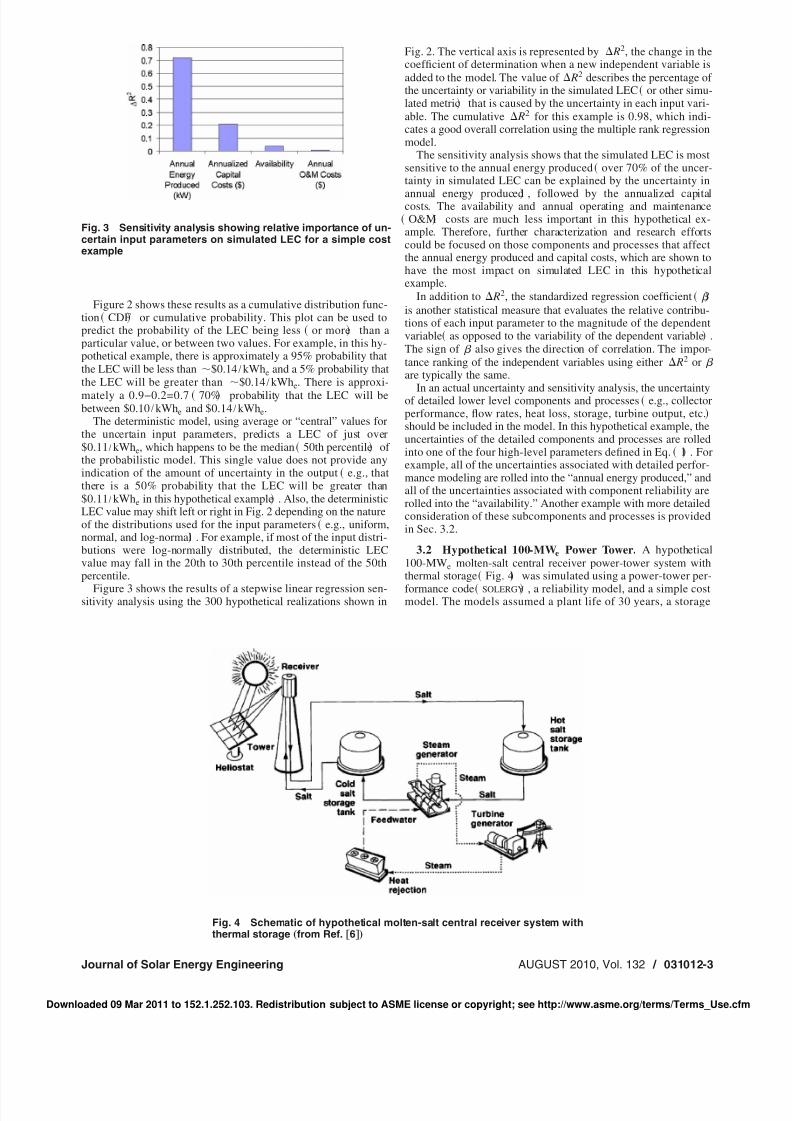
Figure 3 shows the results of a stepwise linear regression sen-sitivity analysis using the 300 hypothetical realizations shown in

Fig. 2. The vertical axis is represented by ⌬ R2, the change in thecoefficient of determination when a new independent variable isadded to the model. The value of ⌬ R2 describes the percentage of the uncertainty or variability in the simulated LEC or other simu-lated metric that is caused by the uncertainty in each input vari-able. The cumulative ⌬ R2 for this example is 0.98, which indi-cates a good overall correlation using the multiple rank regressionmodel.

The sensitivity analysis shows that the simulated LEC is mostsensitive to the annual energy produced over 70% of the uncer-tainty in simulated LEC can be explained by the uncertainty in

annual energy produced , followed by the annualized capitalcosts. The availability and annual operating and maintenance O&M costs are much less important in this hypothetical ex-ample. Therefore, further characterization and research effortscould be focused on those components and processes that affectthe annual energy produced and capital costs, which are shown tohave the most impact on simulated LEC in this hypotheticalexample.

In addition to ⌬ R2, the standardized regression coefficient ␤ is another statistical measure that evaluates the relative contribu-tions of each input parameter to the magnitude of the dependentvariable as opposed to the variability of the dependent variable .The sign of ␤ also gives the direction of correlation. The impor-tance ranking of the independent variables using either ⌬ R2 or ␤ are typically the same.

In an actual uncertainty and sensitivity analysis, the uncertaintyof detailed lower level components and processes e.g., collectorperformance, flow rates, heat loss, storage, turbine output, etc.should be included in the model. In this hypothetical example, theuncertainties of the detailed components and processes are rolledinto one of the four high-level parameters defined in Eq. 1 . Forexample, all of the uncertainties associated with detailed perfor-mance modeling are rolled into the “annual energy produced,” andall of the uncertainties associated with component reliability arerolled into the “availability.” Another example with more detailedconsideration of these subcomponents and processes is providedin Sec. 3.2.

3.2 Hypothetical 100-MWe Power Tower. A hypothetical100-MWe molten-salt central receiver power-tower system withthermal storage Fig. 4 was simulated using a power-tower per-

formance code SOLERGY , a reliability model, and a simple costmodel. The models assumed a plant life of 30 years, a storage

Fig. 3 Sensitivity analysis showing relative importance of un-certain input parameters on simulated LEC for a simple costexample

Fig. 4 Schematic of hypothetical molten-salt central receiver system withthermal storage „from Ref. †6‡…

Journal of Solar Energy Engineering AUGUST 2010, Vol. 132 / 031012-3




capacity of 7 h, and used the 1977 weather data for Barstow, CA,which yielded a direct normal insolation of 2.7 MWh/m2

/yr.Other deterministic parameters used in the models were taken

from Ref. 2 .After an initial screening, a total of 33 parameters were as-

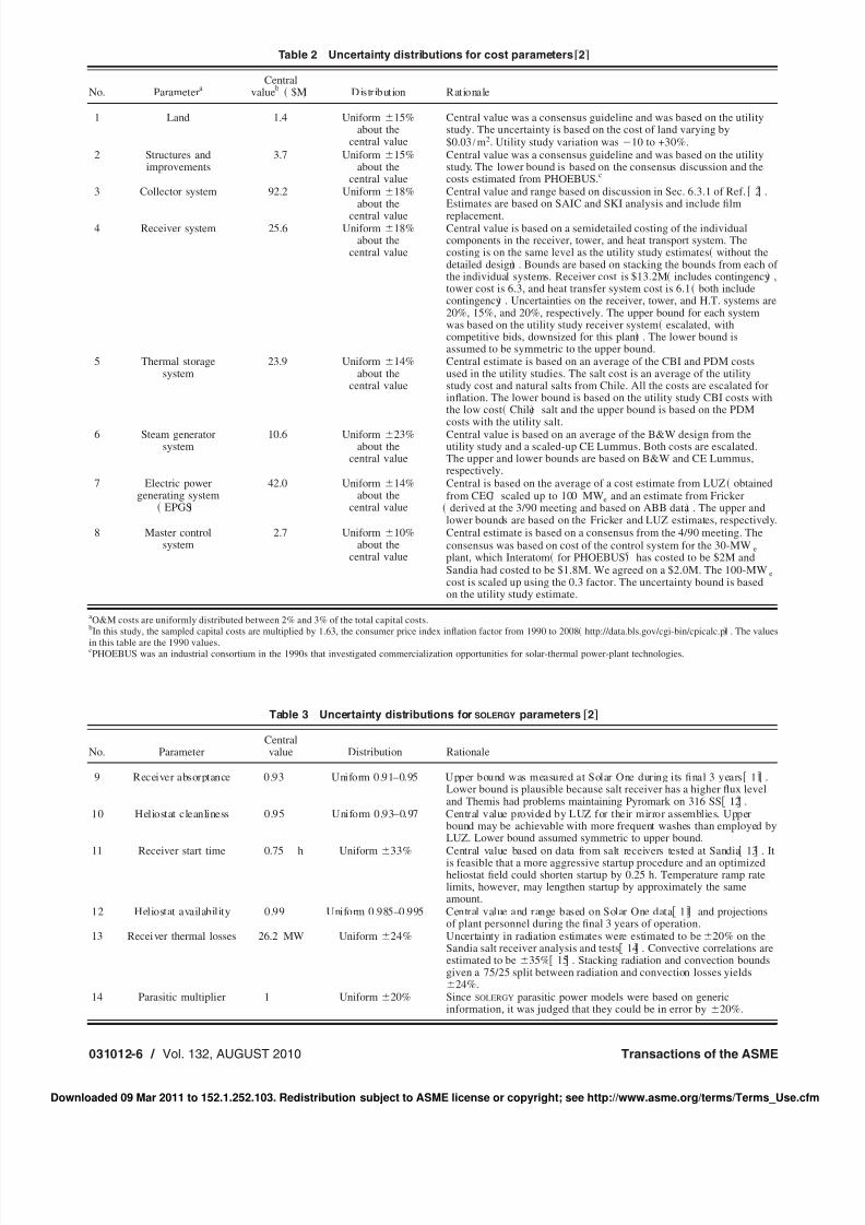
signed uncertainty distributions to represent the inherent uncer-tainty in values associated with costs, the heliostat field, receiver,storage, and power-block components. The uncertain input param-eters are summarized in the Appendix Tables 2–4 ; 32 parametersare defined in the tables, and the 33rd O&M costs is defined inSec. 3.2.1. Sections 3.2.1–3.2.3provide a brief overview of themodels and uncertainties implemented in the analysis.

3.2.1 Cost Model. The cost model that was used is the same asin Eq. 1 , but additional parameters were used to account forindirect charges and financing. The following equation was usedto calculate the annualized capital costs used in Eq. 1 :

Annualized capital costs = FCRϫ DCϫ 1 + INDC

ϫ 1 + AFUDC 2

where FCR=constant-dollar fixed charge rate= 7.4% derivedfrom Ref. 7 , DC= total direct costs, INDC= indirect charges=17% from Ref. 2 , and AFUDC=allowed funds during con-struction to cover interest charges= 6.57% from Ref. 2 .

Uncertain cost parameters used in the model are summarized inTable 2 in the Appendix. It should be noted that the direct costsreported in Ref. 2 were multiplied by an inflation cost index toreflect increases in direct costs from 1990 to 2008. The annualO&M costs were assumed to be a percentage uniformly distrib-uted between 2% and 3% of the direct costs.

3.2.2 SOLERGY Model. SOLERGY 8 simulates the annual en-ergy output of a solar-thermal power plant and has been validatedusing data from Solar One 9 . It utilizes actual or simulatedweather data at time intervals of 15 min and calculates the net

electrical energy output at every time step throughout an entireyear. Input to the code is entered via user-specified text files.

Factors include energy losses in each component of the system,delays incurred during start-up, weather conditions, storage strat-egies, and power limitations for each component. Table 3 summa-rizes the uncertainty distributions used in SOLERGY for this analy-sis. The deterministic value of the total annual energy output

348,018 MWh was calculated using the central values in Table3.

3.2.3 Reliability Model. The reliability model assumes that allof the components act in series if one component goes down, theentire system goes down . The following equation is used to cal-

culate the overall availability A of the system with n componentsbased on the mean time between failure MTBF and mean down

time MDT of each component i:

A =i=1

nMTBFi

MTBFi + MDTi

3

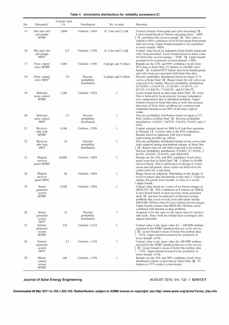
Table 4 in the Appendix summarizes the uncertainty distributionsused in the reliability model. The deterministic value for the totalavailability 0.905 was calculated using the central values listedin Tables 4 and 5.

3.2.4 Results. A total of 64 realizations were implemented us-ing Latin hypercube sampling of the uncertain parameters definedin Tables 2–4 in the Appendix. The 33 parameters were assumedto be independent, and the sample pairings were restricted tominimize the correlations within the LHS model. The number of realizations was sufficient to implement the restricted pairings in

LHS 64Ͼ4k / 3 and to produce reasonable distributions be-

tween the 5th and 95th percentiles for this illustrative example.SOLERGY was run 64 times using the sampled sets of input

parameters. The availability model defined by Eq. 3 was also run64 times using the 64 sets of parameters sampled from the param-eters in Table 4. Finally, the cost model defined by Eqs. 1 and 2was run 64 times using the results from SOLERGY, the availabilitymodel, and the cost parameters listed in Table 2.

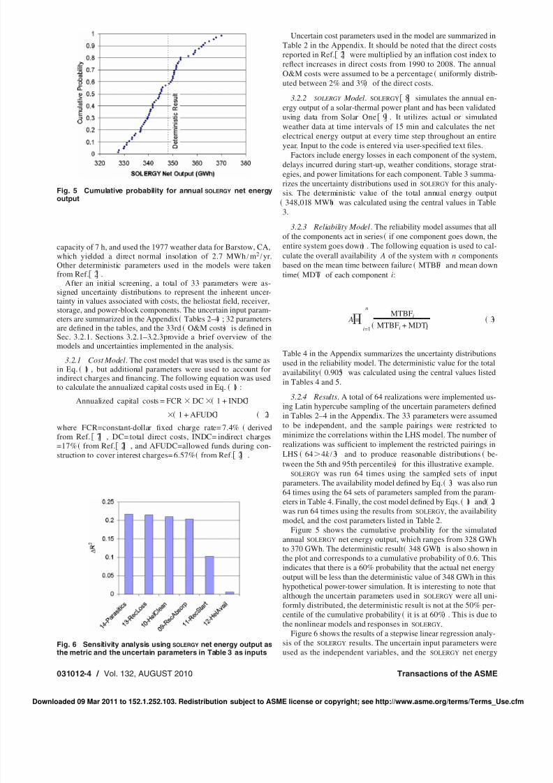
Figure 5 shows the cumulative probability for the simulatedannual SOLERGY net energy output, which ranges from 328 GWh

to 370 GWh. The deterministic result 348 GWh is also shown inthe plot and corresponds to a cumulative probability of 0.6. Thisindicates that there is a 60% probability that the actual net energyoutput will be less than the deterministic value of 348 GWh in thishypothetical power-tower simulation. It is interesting to note thatalthough the uncertain parameters used in SOLERGY were all uni-formly distributed, the deterministic result is not at the 50% per-centile of the cumulative probability it is at 60% . This is due tothe nonlinear models and responses in SOLERGY.

Figure 6 shows the results of a stepwise linear regression analy-sis of the SOLERGY results. The uncertain input parameters wereused as the independent variables, and the SOLERGY net energy

Fig. 5 Cumulative probability for annual SOLERGY net energyoutput

Fig. 6 Sensitivity analysis using SOLERGY net energy output asthe metric and the uncertain parameters in Table 3 as inputs





output was used as the dependent variable. Results show that allsix of the parameters chosen to be represented by uncertaintydistributions were statistically significant, but the parasitics, re-

ceiver heat loss, heliostat cleanliness, and receiver absorptionwere most important. Uncertainties in the heliostat availabilityand receiver start-up time were less important. The cumulative⌬ R2 was 0.96 for the multiple rank regression of simulated netenergy output.

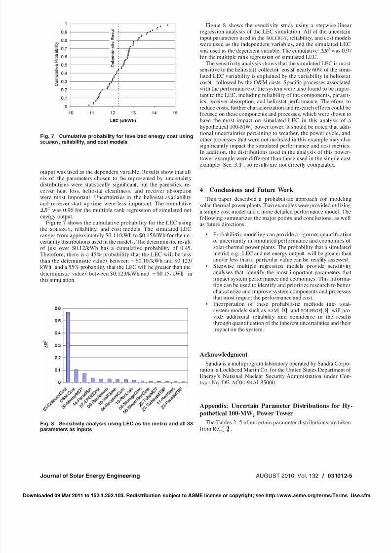
Figure 7 shows the cumulative probability for the LEC usingthe SOLERGY, reliability, and cost models. The simulated LECranges from approximately $0.11/kWh to $0.15/kWh for the un-certainty distributions used in the models. The deterministic resultof just over $0.12/kWh has a cumulative probability of 0.45.Therefore, there is a 45% probability that the LEC will be lessthan the deterministic value between ϳ$0.10 /kWh and $0.123/ kWh and a 55% probability that the LEC will be greater than thedeterministic value between $0.123/kWh and ϳ$0.15 /kWh inthis simulation.

Figure 8 shows the sensitivity study using a stepwise linearregression analysis of the LEC simulation. All of the uncertaininput parameters used in the SOLERGY, reliability, and cost modelswere used as the independent variables, and the simulated LECwas used as the dependent variable. The cumulative ⌬ R2 was 0.97for the multiple rank regression of simulated LEC.

The sensitivity analysis shows that the simulated LEC is mostsensitive to the heliostat collector costs nearly 60% of the simu-lated LEC variability is explained by the variability in heliostatcosts , followed by the O&M costs. Specific processes associatedwith the performance of the system were also found to be impor-

tant to the LEC, including reliability of the components, parasit-ics, receiver absorption, and heliostat performance. Therefore, toreduce costs, further characterization and research efforts could befocused on these components and processes, which were shown tohave the most impact on simulated LEC in this analysis of ahypothetical 100-MWe power tower. It should be noted that addi-tional uncertainties pertaining to weather, the power cycle, andother processes that were not included in this example may alsosignificantly impact the simulated performance and cost metrics.In addition, the distributions used in the analysis of this power-tower example were different than those used in the simple costexample Sec. 3.1 , so results are not directly comparable.

4 Conclusions and Future Work

This paper described a probabilistic approach for modelingsolar-thermal power plants. Two examples were provided utilizinga simple cost model and a more detailed performance model. Thefollowing summarizes the major points and conclusions, as wellas future directions.

• Probabilistic modeling can provide a rigorous quantificationof uncertainty in simulated performance and economics of solar-thermal power plants. The probability that a simulatedmetric e.g., LEC and net energy output will be greater thanand/or less than a particular value can be readily assessed.

• Stepwise multiple regression models provide sensitivityanalyses that identify the most important parameters thatimpact system performance and economics. This informa-tion can be used to identify and prioritize research to better

characterize and improve system components and processesthat most impact the performance and cost.

• Incorporation of these probabilistic methods into total-system models such as SAM 10 and SOLERGY 8 will pro-vide additional reliability and confidence in the resultsthrough quantification of the inherent uncertainties and theirimpact on the system.

Acknowledgment

Sandia is a multiprogram laboratory operated by Sandia Corpo-ration, a Lockheed Martin Co. for the United States Department of Energy’s National Nuclear Security Administration under Con-tract No. DE-AC04-94AL85000.

Appendix: Uncertain Parameter Distributions for Hy-

pothetical 100-MWe Power Tower

The Tables 2–5 of uncertain parameter distributions are takenfrom Ref. 2 .

Fig. 7 Cumulative probability for levelized energy cost usingSOLERGY, reliability, and cost models

Fig. 8 Sensitivity analysis using LEC as the metric and all 33parameters as inputs





Table 2 Uncertainty distributions for cost parameters †2‡

No. ParameteraCentral

valueb $M Distribution Rationale

1 Land 1.4 Uniform Ϯ15%about the

central value

Central value was a consensus guideline and was based on the utilitystudy. The uncertainty is based on the cost of land varying by$0.03/m2. Utility study variation was Ϫ10 to +30%.

2 Structures andimprovements

3.7 Uniform Ϯ15%about the

central value

Central value was a consensus guideline and was based on the utilitystudy. The lower bound is based on the consensus discussion and thecosts estimated from PHOEBUS.c

3 Collector system 92.2 Uniform Ϯ18%about the

central value

Central value and range based on discussion in Sec. 6.3.1 of Ref. 2 .Estimates are based on SAIC and SKI analysis and include film

replacement.4 Receiver system 25.6 Uniform Ϯ18%

about thecentral value

Central value is based on a semidetailed costing of the individualcomponents in the receiver, tower, and heat transport system. Thecosting is on the same level as the utility study estimates without thedetailed design . Bounds are based on stacking the bounds from each of the individual systems. Receiver cost is $13.2M includes contingency ,tower cost is 6.3, and heat transfer system cost is 6.1 both includecontingency . Uncertainties on the receiver, tower, and H.T. systems are20%, 15%, and 20%, respectively. The upper bound for each systemwas based on the utility study receiver system escalated, withcompetitive bids, downsized for this plant . The lower bound isassumed to be symmetric to the upper bound.

5 Thermal storagesystem


central value

Central estimate is based on an average of the CBI and PDM costsused in the utility studies. The salt cost is an average of the utilitystudy cost and natural salts from Chile. All the costs are escalated forinflation. The lower bound is based on the utility study CBI costs withthe low cost Chile salt and the upper bound is based on the PDMcosts with the utility salt.

6 Steam generatorsystem


central value

Central value is based on an average of the B&W design from theutility study and a scaled-up CE Lummus. Both costs are escalated.The upper and lower bounds are based on B&W and CE Lummus,respectively.

7 Electric powergenerating system

EPGS


central value

Central is based on the average of a cost estimate from LUZ obtainedfrom CEC scaled up to 100 MWe and an estimate from Fricker

derived at the 3/90 meeting and based on ABB data . The upper andlower bounds are based on the Fricker and LUZ estimates, respectively.

8 Master controlsystem


central value

Central estimate is based on a consensus from the 4/90 meeting. Theconsensus was based on cost of the control system for the 30-MW e

plant, which Interatom for PHOEBUSc has costed to be $2M andSandia had costed to be $1.8M. We agreed on a $2.0M. The 100-MW e

cost is scaled up using the 0.3 factor. The uncertainty bound is basedon the utility study estimate.

aO&M costs are uniformly distributed between 2% and 3% of the total capital costs.bIn this study, the sampled capital costs are multiplied by 1.63, the consumer price index inflation factor from 1990 to 2008 http://data.bls.gov/cgi-bin/cpicalc.pl . The values

in this table are the 1990 values.cPHOEBUS was an industrial consortium in the 1990s that investigated commercialization opportunities for solar-thermal power-plant technologies.

Table 3 Uncertainty distributions for SOLERGY parameters †2‡

No. ParameterCentral

value Distribution Rationale

9 Receiver absorptance 0.93 Uniform 0.91–0.95 Upper bound was measured at Solar One during its final 3 years 11 .Lower bound is plausible because salt receiver has a higher flux leveland Themis had problems maintaining Pyromark on 316 SS 12 .

10 Heliostat cleanliness 0.95 Uniform 0.93–0.97 Central value provided by LUZ for their mirror assemblies. Upperbound may be achievable with more frequent washes than employed byLUZ. Lower bound assumed symmetric to upper bound.

11 Receiver start time 0.75 h Uniform Ϯ33% Central value based on data from salt receivers tested at Sandia

13

. Itis feasible that a more aggressive startup procedure and an optimizedheliostat field could shorten startup by 0.25 h. Temperature ramp ratelimits, however, may lengthen startup by approximately the sameamount.

12 Heliostat availability 0.99 Uniform 0.985–0.995 Central value and range based on Solar One data 11 and projectionsof plant personnel during the final 3 years of operation.

13 Receiver thermal losses 26.2 MW Uniform Ϯ24% Uncertainty in radiation estimates were estimated to be Ϯ20% on theSandia salt receiver analysis and tests 14 . Convective correlations areestimated to be Ϯ35% 15 . Stacking radiation and convection boundsgiven a 75/25 split between radiation and convection losses yieldsϮ24%.

14 Parasitic multiplier 1 Uniform Ϯ20% Since SOLERGY parasitic power models were based on genericinformation, it was judged that they could be in error by Ϯ20%.





Table 4 Uncertainty distributions for reliability parameters †2‡

No. Para meteraCentral value

h Distribution No. of units Rationale

15 Hot and coldsalt pumps

MTBF

2,800 Uniform Ϯ60% 4 2 hot and 2 cold Central estimate from pump and valve loop data 16 .Lower bound based on Themis salt pump data Ϫ60%

17 and Solar One receiver pump 18 . This value issimilar to 90% confidence level for hot pump from pumpand valve loop. Upper bound assumed to be symmetricto lower bound +60% .

16 Hot and coldsalt pumps

MDTb

6.5 Uniform Ϯ70% 4 2 hot and 2 cold Central value based on judgments from Sandia pump andvalve loop personnel. Lower bound based on mean value

for Solar One receiver pump Ϫ70% 18 . Upper boundassumed to be symmetric to lower bound +70% .

17 Flow controlvalve MTBF

3,460 Uniform Ϯ20% 4 pumps and 5 others Bounds are the 10% and 90% confidence levels fromFCV data at Solar One 31 failures in 104,000 valvehours 18 . Limited FCV failure data from Sandia pumpand valve loop are consistent with Solar One data.

18 Flow controlvalve MDT

b2.9 Discrete

probabilitydistribution

4 pumps and 5 others Discrete probability distribution based on repair of 31valves at Solar One 18 . Repair times for salt valves areexpected to be similar. Discrete probability distribution:0.5 h/29%, 1.5 h/19.4%, 2.5 h/16%, 3.5 h/13%, 4.5h/3.2%, 6.5 h/6.5%, 7.5 h/6.5%, and 8.5 h/6.5%.

19 Heliostatarray control

MTBF

1,284 Uniform Ϯ82% 1 Lower bound based on data from Solar One 18 . SolarOne is believed to be pessimistic because redundancywas compromised due to identified problems. Upperbound is based on Solar One data as well, but assumesthat most of Solar One’s problems are corrected andredundant backup occurs 90% of the time typicalvalue

.

20 Heliostatarray control

MDT

3.3 Discreteprobabilitydistribution

1 Discrete probability distribution based on repair of 25HAC failures at Solar One 18 . Discrete probabilitydistribution: 1 h/36%, 3 h/32%, 5 h/24%, 9 h/4%, and 13h/4%.

21 Receivertube leak

MTBF

4,166 Uniform Ϯ50% 1 Central estimate based on 3000 h of leak-free operationat Themis 17 . Central value is the 50% confidence.Bounds based on judgment with lower boundrepresenting possible age effects.

22 Receivertube leak

MDT

14 Discreteprobabilitydistribution

1 Discrete probability distribution based on ten severe tubeleaks repaired during unscheduled outages at Solar One

18 . Repair time for salt tubes expected to be similar.Discrete probability distribution: 0 h/40%, 0.7 h/10%, 3h/10%, 8 h/20%, 13 h/10%, and 108 h/10%.

23 Warpedreceiver

panel MTBF

10,000 Uniform Ϯ80% 1 Bounds are the 10% and 90% confidence levels frompanel warp data at Solar One 18 1 failure in 10,000receiver hours . Due to differences in design of water/ steam and salt panels, these values are believed to be

conservative for a salt plant.24 Warped

receiverpanel MDT

46 Uniform Ϯ80% 1 Range based on judgment. Depending on the design of receiver panels and attachments it may take 1–2 days toreplace the panel lower bound or close to 2 weeks

upper bound .25 Steam

generatorsystemMTBF

9,500 Uniform Ϯ90% 1 Central value based on 3 years of no forced outages atSEGS IV 19 50% confidence of 0 failures in 7000 h .Lower bound based on heat recovery steam generatordata 20 and may be indicative of thermal cyclingproblems that occur several years after plant startup.SEGS III–VII have had 10 years with no forced outages.Upper bound assumes that SEGS III–VII data can becombined with thermal cycling problems.

26 Steamgenerator

systemMDT

14 Discreteprobabilitydistribution

1 Assumed to be the same as the repair time for receivertube leaks. Since both are tubular heat exchangers, thisappears plausible.

27 Turbine

generatorsystemMTBF

319 Uniform Ϯ41% 1 Central value is the mean value for Ϫ100-MW turbines

reported in the NERC database that see cyclic service 20 . Lower bound is mean of Solar One turbine data Ϫ41% . Upper bound assumed to be symmetric tolower bound +41% .

28 Turbinegenerator

systemMDT

3.3 Uniform Ϯ33% 1 Central value is the mean value for 100-MW turbinesreported in the NERC database that see cyclic service

20 . Lower bound is mean of Solar One turbine data Ϫ33% . Upper bound assumed to be symmetric tolower bound +33% .

29 MastercontrolsystemMTBF

165 Uniform Ϯ19% 1 Bounds are the 10% and 90% confidence levels fromdistributed control system data at Solar One 18 35failures in 5774 control system hours .





References 1 U.S. Code of Federal Regulations, 2008, “Requirements for Performance As-

sessment,” Title 10, Part 63, Section 114. 2 1993, Second-Generation Central Receiver Technologies: A Status Report , M.

Becker and P. C. Klimas, eds., C.F. Muller, Karlsruhe, Germany. 3 Wyss, G. D., and Jorgensen, K. H., 1998, “A User’s Guide to LHS: Sandia’s

Latin Hypercube Sampling Software,” Sandia National Laboratories, ReportNo. SAND98-0210.

4 Blower, S. M., and Dowlatabadi, H., 1994, “Sensitivity and UncertaintyAnalysis of Complex Models of Disease Transmission: An HIV Model, as anExample,” Int. Statist. Rev., 62 2 , pp. 229–243.

5 Helton, J. C., and Davis, F. J., 2000, “Sampling-Based Methods for Uncer-tainty and Sensitivity Analysis,” Sandia National Laboratories, Report No.SAND99-2240.

6 Falcone, P. K., 1986, “A Handbook for Solar Central Receiver Design,” SandiaNational Laboratories, Report No. SAND86-8009.

7 Sargent & Lundy Consulting Group, 2003, “Assessment of Parabolic Troughand Power Tower Solar Technology Cost and Performance Forecasts,” ReportNo. SL-5641.

8 Stoddard, M. C., Faas, S. E., Chiang, C. J., and Dirks, J. A., 1987,“SOLERGY—A Computer Code for Calculating the Annual Energy FromCentral Receiver Power Plants,” Sandia National Laboratories, Report No.SAND86-8060.

9 Alpert, D. J., and Kolb, G. J., 1988, “Performance of the Solar One PowerPlant as Simulated by the SOLERGY Computer Code,” Sandia National Labo-ratories, Report No. SAND88-0321.

10 Gilman, P., Blair, N., Mehos, M., Christenson, C., Janzou, S., and Cameron,

C., 2008, “Solar Advisor Model User Guide for Version 2.0,” National Renew-able Energy Laboratory, Report No. NREL/TP-670-43704.

11 Radosevich, L. G., 1988, “Final Report on the Power Production Phase of the

10 MWe Solar Thermal Central Receiver Pilot Plant,” Sandia National Labo-ratories, Report No. SAND87-8022.

12 Etievant, C., 1988, “Central Receiver Plant Evaluation III, Themis ReceiverSubsystem Evaluation,” Sandia National Laboratories, Report No. SAND88-8101.

13 Smith, D. C., and Chavez, J. M., 1988, A Final Report on the Phase 1 Testingof a Molten-Salt Cavity Receiver – Volume 1 – A Summary Report, Sandia

National Laboratories, Report No. SAND87-2290. 14 Boehm, R., Nakhaie, H., and Berg, D., Jr., 1988, “Heat Loss Experiments onthe Category B Solar Receiver,” Proceedings of the Tenth Annual ASME SolarEnergy Conference, Denver, CO, Apr. 10–14.

15 Siebers, D. L., and Kraabel, J. S., 1986, “Estimating Convective EnergyLosses From Solar Central Receivers,” Sandia National Laboratories, ReportNo. SAND84-8717.

16 Rush, E. E., Jr., Chavez, J. M., Smith, D. C., and Matthews, C. W., 1991,“Report on Tests of the Molten Salt Pump and Valve Loops,” Proceedings of the ASME Solar Energy Conference, Reno, NV, Apr.

17 Pharabod, F., Bezian, J. J., Bonduelle, B., Rivoire, B., and Guillard, J., 1986,“Themis Evaluation Report,” Proceedings of the Third International Workshop

on Solar-Thermal Central Receiver Systems: Volume 1, Springer-Verlag, Ber-lin.

18 Kolb, G. J., and Lopez, C. W., 1988, “Reliability of the Solar One Plant Duringthe Power Production Phase,” Sandia National Laboratories, Report No.SAND88-2664.

19 Price, H., 1990, private communication. 20 North American Electric Reliability Council NERC , 1989, “Data Reporting

Instructions for Generating Availability Data System,” data scan for coolwatercombined-cycle plants from 1982 to 1988, Princeton, NJ, Oct.

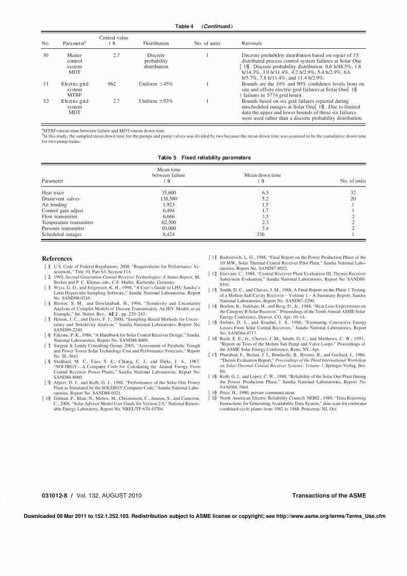
Table 5 Fixed reliability parameters

Parameter

Mean timebetween failure

hMean down time

h No. of units

Heat trace 35,600 6.5 32Drain/vent valves 138,580 5.2 20Air binding 1,923 1.5 1Control gain adjust 6,494 1.7 1Flow transmitter 6,666 3.5 2Temperature transmitter 62,500 2.3 2Pressure transmitter 10,000 3.4 2Scheduled outages 8,424 336 1

Table 4 „Continued.…

No. Para meteraCentral value

h Distribution No. of units Rationale

30 MastercontrolsystemMDT

2.7 Discreteprobabilitydistribution

1 Discrete probability distribution based on repair of 35distributed process control system failures at Solar One

18 . Discrete probability distribution: 0.6 h/48.5%, 1.8h/14.3%, 3.0 h/11.4%, 4.2 h/2.9%, 5.4 h/2.9%, 6.6h/5.7%, 7.8 h/11.4%, and 11.4 h/2.9%.

31 Electric gridsystemMTBF

962 Uniform Ϯ45% 1 Bounds are the 10% and 90% confidence levels from onsite and offsite electric grid failures at Solar One 18

failures in 5774 grid hours .

32 Electric gridsystemMDT

2.7 Uniform Ϯ93% 1 Bounds based on six grid failures repaired duringunscheduled outages at Solar One 18 . Due to limiteddata the upper and lower bounds of these six failureswere used rather than a discrete probability distribution.

aMTBF=mean time between failure and MDT=mean down time.bIn this study, the sampled mean down time for the pumps and pump valves was divided by two because the mean down time was assumed to be the cumulative down timefor two pump trains.


Documents

Probabilistic Performance Models of Solar Plants 8pp