Probability Concepts and Applications - Bilal Bajwa

4

TEACHING SUGGESTIONS

Teaching Suggestion 2.1: Concept of Probabilities Ranging From 0 to 1.People often misuse probabilities by such statements as, “I’m110% sure we’re going to win the big game.” The two basic rulesof probability should be stressed.

Teaching Suggestion 2.2: Where Do Probabilities Come From?Students need to understand where probabilities come from.Sometimes they are subjective and based on personal experiences.Other times they are objectively based on logical observationssuch as the roll of a die. Often, probabilities are derived from his-torical data—if we can assume the future will be about the same asthe past.

Teaching Suggestion 2.3: Confusion Over Mutually Exclusiveand Collectively Exhaustive Events.This concept is often foggy to even the best of students—even ifthey just completed a course in statistics. Use practical examplesand drills to force the point home. The table at the end of Example3 is especially useful.

Teaching Suggestion 2.4: Addition of Events That Are NotMutually Exclusive.The formula for adding events that are not mutually exclusive isP(A or B) � P(A) � P(B) � P(A and B). Students must understandwhy we subtract P(A and B). Explain that the intersect has beencounted twice.

Teaching Suggestion 2.5: Statistical Dependence with Visual Examples.Figure 2.3 indicates that an urn contains 10 balls. This exampleworks well to explain conditional probability of dependent events.An even better idea is to bring 10 golf balls to class. Six should bewhite and 4 orange (yellow). Mark a big letter or number on eachto correspond to Figure 2.3 and draw the balls from a clear bowl tomake the point. You can also use the props to stress how randomsampling expects previous draws to be replaced.

Teaching Suggestion 2.6: Concept of Random Variables.Students often have problems understanding the concept of ran-dom variables. Instructors need to take this abstract idea and pro-vide several examples to drive home the point. Table 2.2 has someuseful examples of both discrete and continuous random variables.

Teaching Suggestion 2.7: Expected Value of a Probability Distribution.A probability distribution is often described by its mean and variance. These important terms should be discussed with such

practical examples as heights or weights of students. But studentsneed to be reminded that even if most of the men in class (or theUnited States) have heights between 5 feet 6 inches and 6 feet 2inches, there is still some small probability of outliers.

Teaching Suggestion 2.8: Bell-Shaped Curve.Stress how important the normal distribution is to a large numberof processes in our lives (for example, filling boxes of cereal with32 ounces of cornflakes). Each normal distribution depends on themean and standard deviation. Discuss Figures 2.8 and 2.9 to showhow these relate to the shape and position of a normal distribution.

Teaching Suggestion 2.9: Three Symmetrical Areas Under theNormal Curve.Figure 2.10 is very important, and students should be encouragedto truly comprehend the meanings of �1, 2, and 3 standard devia-tion symmetrical areas. They should especially know that man-agers often speak of 95% and 99% confidence intervals, whichroughly refer to �2 and 3 standard deviation graphs. Clarify that95% confidence is actually �1.96 standard deviations, while �3standard deviations is actually a 99.7% spread.

Teaching Suggestion 2.10: Using the Normal Table to AnswerProbability Questions.The IQ example in Figure 2.11 is a particularly good way to treatthe subject since everyone can relate to it. Students are typicallycurious about the chances of reaching certain scores. Go throughat least a half-dozen examples until it’s clear that everyone canuse the table. Students get especially confused answering ques-tions such as P(X � 85) since the standard normal table showsonly right-hand-side Z values. The symmetry requires special care.

ALTERNATIVE EXAMPLES

Alternative Example 2.1: In the past 30 days, Roger’s RuralRoundup has sold either 8, 9, 10, or 11 lottery tickets. It never soldfewer than 8 nor more than 11. Assuming that the past is similar tothe future, here are the probabilities:

Alternative Example 2.2: Grades received for a course have aprobability based on the professor’s grading pattern. Here are Pro-fessor Ernie Forman’s BA205 grades for the past five years.

2C H A P T E R

Probability Concepts and Applications

Sales No. Days Probability

8 10 0.3339 12 0.400

10 6 0.20011 2 0.067Total 30 1.000

M02_REND6289_10_IM_C02.QXD 5/7/08 2:31 PM Page 4REVISED

CHAPTER 2 PROBABIL ITY CONCEPTS AND APPL ICAT IONS 5

1 2 3 4 5

Possible Outcomes, x

0.4

0.3

0.2

0.1

Pro

babi

lity

These grades are mutually exclusive and collectively exhaustive.

Alternative Example 2.3:

P(drawing a 3 from a deck of cards) � 4/52 � 1/13

P(drawing a club on the same draw) � 13/52 � 1/4

These are neither mutually exclusive nor collectively exhaustive.

Alternative Example 2.4: In Alternative Example 2.3 welooked at 3s and clubs. Here is the probability for 3 or club:

P(3 or club) � P(3) � P(club) � P(3 and club)

� 4/52 � 13/52 � 1/52

� 16/52 � 4/13

Alternative Example 2.5: A class contains 30 students. Ten arefemale (F) and U.S. citizens (U); 12 are male (M) and U.S. citi-zens; 6 are female and non-U.S. citizens (N); 2 are male and non-U.S. citizens.

A name is randomly selected from the class roster and it isfemale. What is the probability that the student is a U.S. citizen?

U.S. Not U.S. Total

F 10 6 16M 12 2 14Total 22 8 30

P(U | F) = 10/16

Alternative Example 2.6: Your professor tells you that if youscore an 85 or better on your midterm exam, there is a 90% chanceyou’ll get an A for the course. You think you have only a 50%chance of scoring 85 or better. The probability that both yourscore is 85 or better and you receive an A in the course is

P(A and 85) � P(A � 85) � P(85) � (0.90)(0.50) � 0.45

� 45%

Alternative Example 2.7: An instructor is teaching two sec-tions (classes) of calculus. Each class has 24 students, and on thesurface, both classes appear identical. One class, however, consistsof students who have all taken calculus in high school. The in-structor has no idea which class is which. She knows that the prob-ability of at least half the class getting As on the first exam is only 25% in an average class, but 50% in a class with more mathbackground.

A section is selected at random and quizzed. More than halfthe class received As. Now, what is the revised probability that theclass was the advanced one?

P(regular class chosen) � 0.5

P(advanced class chosen) � 0.5

P(�1/2 As � regular class) � 0.25

P(�1/2 As � advanced class) � 0.50

P(�1/2 As and regular class)

� P(�1/2 As � regular ) � P(regular)

� (0.25)(0.50) � 0.125

P(�1/2 As and advanced class)

� P(�1/2 As � advanced) � P(advanced)

� (0.50)(0.5) � 0.25

So P(�1/2 As) � 0.125 � 0.25 � 0.375

So there is a 66% chance the class tested was the advancedone.

Alternative Example 2.8: Students in a statistics class wereasked how many “away” football games they expected to attend inthe upcoming season. The number of students responding to eachpossibility are shown below:

Number of games Number of students

5 404 303 202 101 0

100

A probability distribution of the results would be:

Number of games Probability P(X)

5 0.4 � 40/1004 0.3 � 30/1003 0.2 � 20/1002 0.1 � 10/1001 0.0 � 0/100

1.0 � 100/100

This discrete probability distribution is computed using the rela-tive frequency approach. Probabilities are shown in graph formbelow.

� �0 25

0 3752 3

.

./

PP

(advanced As(advanced and As

� >>

1 21 2

/ )/ )

�PP( / )> 1 2 As

Outcome Probability

A 0.25B 0.30C 0.35D 0.03F 0.02

Withdraw/drop 0.051.00


6 CHAPTER 2 PROBABIL ITY CONCEPTS AND APPL ICAT IONS

Alternative Example 2.9: Here is how the expected outcomecan be computed for the question in Alternative Example 2.8.

� x3P(x3) �x4P(x4) � x5P(x5)

� 5(0.4) � 4(0.3) � 3(0.2) � 2(0.1) � 1(0)

� 4.0

Alternative Example 2.10: Here is how variance is computedfor the question in Alternative Example 2.8:

� (5 � 4)2(0.4) � (4 � 4)2(0.3) � (3 � 4)2(0.2) � (2 � 4)2(0.1) � (1 � 4)2(0)

� (1)2(0.4) � (0)2(0.3) � (�1)2(0.2) � (�2)2(0.1)

� 0.4 � 0.0 � 0.2 � 0.4 � 0.0

� 1.0

The standard deviation is

�1

Alternative Example 2.11: The length of the rods coming outof our new cutting machine can be said to approximate a normaldistribution with a mean of 10 inches and a standard deviation of0.2 inch. Find the probability that a rod selected randomly willhave a length

a. of less than 10.0 inchesb. between 10.0 and 10.4 inchesc. between 10.0 and 10.1 inchesd. between 10.1 and 10.4 inchese. between 9.9 and 9.6 inchesf. between 9.9 and 10.4 inchesg. between 9.886 and 10.406 inches

First compute the standard normal distribution, the Z-value:

Next, find the area under the curve for the given Z-value by usinga standard normal distribution table.

a. P(x � 10.0) � 0.50000b. P(10.0 � x � 10.4) � 0.97725 � 0.50000 � 0.47725c. P(10.0 � x � 10.1) � 0.69146 � 0.50000 � 0.19146d. P(10.1 � x � 10.4) � 0.97725 � 0.69146 � 0.28579e. P(9.6 � x � 9.9) � 0.97725 � 0.69146 � 0.28579f. P(9.9 � x � 10.4) � 0.19146 � 0.47725 � 0.66871g. P(9.886 � x � 10.406) � 0.47882 � 0.21566 �

0.69448

SOLUTIONS TO DISCUSSION QUESTIONS

AND PROBLEMS

2-1. There are two basic laws of probability. First, the probabilityof any event or state of nature occurring must be greater than or equalto zero and less than or equal to 1. Second, the sum of the simpleprobabilities for all possible outcomes of the activity must equal 1.

zx

��μσ

= 1

σ = variance

variance� �i

i ix E x P x=

−1

52( ( )) ( )

E x x P x x P x x P xi

i i( ) ( ) ( ) ( )= = +=�

1

5

1 1 2 2

2-2. Events are mutually exclusive if only one of the events canoccur on any one trial. Events are collectively exhaustive if the listof outcomes includes every possible outcome. An example of mu-tually exclusive events can be seen in flipping a coin. The outcomeof any one trial can either be a head or a tail. Thus, the events ofgetting a head and a tail are mutually exclusive because only oneof these events can occur on any one trial. This assumes, ofcourse, that the coin does not land on its edge. The outcome ofrolling the die is an example of events that are collectively exhaus-tive. In rolling a standard die, the outcome can be either 1, 2, 3, 4,5, or 6. These six outcomes are collectively exhaustive becausethey include all possible outcomes. Again, it is assumed that thedie will not land and stay on one of its edges.

2-3. Probability values can be determined both objectively andsubjectively. When determining probability values objectively,some type of numerical or quantitative analysis is used. When de-termining probability values subjectively, a manager’s or decisionmaker’s judgment and experience are used in assessing one ormore probability values.

2-4. The probability of the intersection of two events is sub-tracted in summing the probability of the two events to avoiddouble counting. For example, if the same event is in both of theprobabilities that are to be added, the probability of this event willbe included twice unless the intersection of the two events is sub-tracted from the sum of the probability of the two events.

2-5. When events are dependent, the occurrence of one eventdoes have an effect on the probability of the occurrence of theother event. When the events are independent, on the other hand,the occurrence of one of them has no effect on the probability ofthe occurrence of the other event. It is important to know whetheror not events are dependent or independent because the probabilityrelationships are slightly different in each case. In general, theprobability relationships for any kind of independent events aresimpler than the more generalized probability relationships fordependent events.

2-6. Bayes’ theorem is a probability relationship that allowsnew information to be incorporated with prior probability valuesto obtain updated or posterior probability values. Bayes’ theoremcan be used whenever there is an existing set of probability valuesand new information is obtained that can be used to revise theseprobability values.

2-7. A Bernoulli process has two possible outcomes, and the probability of occurrence is constant from one trial to the next.If n independent Bernoulli trials are repeated and the number of outcomes (successes) are recorded, the result is a binomial distribution.

2-8. A random variable is a function defined over a sample space.There are two types of random variables: discrete and continuous.

The distributions for the price of a product, the number ofsales for a salesperson, and the number of ounces in a food con-tainer are examples of a probability distribution.

2-9. A probability distribution is a statement of a probabilityfunction that assigns all the probabilities associated with a randomvariable. A discrete probability distribution is a distribution of dis-crete random variables (that is, random variables with a limited setof values). A continuous probability distribution is concerned witha random variable having an infinite set of values.



a. The probability of getting a 4-inch nail is

� 0.26

b. The probability of getting a 5-inch nail is

� 0.19

c. The probability of getting a nail 3 inches or shorter is theprobability of getting a nail 1 inch, 2 inches, or 3 inches inlength. The probability is thus

P(1 or 2 or 3)

� P(1) � P(2) � P(3)

� 0.38 � 0.14 � 0.02

� 0.54

� � �651

1 719

243

1 719

41

1 719, , ,

P( ),

5333

1 719�

P( ),

4451

1 719�

Type of Nail Number in Bin

1 inch 6512 inch 2433 inch 414 inch 4515 inch 333

Total 1,719

(the events aremutually exclusive)

2-10. The expected value is the average of the distribution and iscomputed by using the following formula: E(X) � �X · P(X) (thisis for a discrete probability distribution).

2-11. The variance is a measure of the dispersion of the distribu-tion. The variance of a discrete probability distribution is com-puted by the formula

V � �[X � E(X)]2 · P(X)

2-12. The purpose of this question is to have students name threebusiness processes they know that can be described by a normaldistribution. Answers could include sales of a product, projectcompletion time, average weight of a product, and product de-mand during lead or order time.

2-13. This is an example of a discrete probability distribution. Itwas most likely computed using historical data. It is important tonote that it follows the laws of a probability distribution. The totalsums to 1, and the individual values are less than or equal to 1.

2-14.

2-16. The distribution of chips is as follows:

Red 8Green 10White 22

Total � 20

a. The probability of drawing a white chip on the first draw is

b. The probability of drawing a white chip on the first drawand a red one on the second is

P(WR) � P(W) � P(R)

� (0.10)(0.40)

� 0.04c. P(GG) � P(G) � P(G)

� (0.5)(0.5)

� 0.25

d. P(R � W) � P(R)

� 0.40

2-17. The distribution of the nails is as follows:

= 8

20

= 10

20

10

20�

� �2

20

8

20

P W( ) .� � �2

20

1

100 10

(the two events are independent)

(the events are independent and hence the conditionalprobability equals the marginalprobability)

Grade Probability

A

B

C

D

F

1.0

0.0825

300=

⎛⎝⎜

⎞⎠⎟

0.1030

300=

⎛⎝⎜

⎞⎠⎟

0.3090

300=

⎛⎝⎜

⎞⎠⎟

0.2575

300=

⎛⎝⎜

⎞⎠⎟

0.2780

300�

⎛⎝⎜

⎞⎠⎟

Thus, the probability of a student receiving a C in the course is0.30 � 30%.

The probability of a student receiving a C may also be calcu-lated using the following equation:

� 0.30

2-15. a. P(H) � 1/2 � 0.5b. P(T � H) � P(T) � 0.5c. P(TT) � P(T) � P(T) � (0.5)(0.5) � 0.25d. P(TH) � P(T) � P(H) � (0.5)(0.5) � 0.25e. We first calculate P(TH) � 0.25, then calculate P(HT) �

(0.5)(0.5) � 0.25. To find the probability of either one occur-ring, we simply add the two probabilities. The solution is 0.50.

f. At least one head means that we have either HT, TH, orHH. Since each of these have a probability of 0.25, their totalprobability of occurring is 0.75. On the other hand, the com-plement of the outcome “at least one head” is “two tails.”Thus, we could have also computed the probability from 1 �P(TT) � 1 � 0.25 � 0.75.

P(C)�90

300

P(of receiving a C) =no. students receiving aa C

total no. students



2-18.

Exercise No Exercise Total

Cold 45 155 200No cold 455 345 800Total 500 500 1000

a. The probability that an employee will have a cold nextyear is

� .20

b. The probability that an employee who is involved in anexercise program will get a cold is

� .09

c. The probability that an employee who is not involved inan exercise program will get a cold is

� .31

d. No. If they were independent, then

P(C � E) � P(C), but

� 0.2Therefore, these events are dependent.

2-19. The probability of winning tonight’s game is

� 0.6The probability that the team wins tonight is 0.60. The probabilitythat the team wins tonight and draws a large crowd at tomorrow’sgame is a joint probability of dependent events. Let the probabilityof winning be P(W) and the probability of drawing a large crowdbe P(L). Thus

P(WL) � P(L � W) � P(W) (the probability of� 0.90 � 0.60 large crowd is 0.90 if� 0.54 the team wins tonight)

Thus, the probability of the team winning tonight and of therebeing a large crowd at tomorrow’s game is 0.54.

2-20. The second draw is not independent of the first because theprobabilities of each outcome depend on the rank (sophomore orjunior) of the first student’s name drawn. Let

�6

10

number of wins

number of games�

12

20

P C( ),

�200

1 000

P C E( ) .� � �45

5000 09

�155

500

P C NP CN

P N( | )

( )

( )�

�45

500

P C EP CE

P E( )

( )

( )� �

�200

1 000,

P C( ) �Number of people who had colds

Total nummber of employees

J1 � junior on first drawJ2 � junior on second drawS1 � sophomore on first drawS2 � sophomore on second draw

a. P(J1) � 3/10 � 0.3b. P(J2 � S1) � 0.3c. P(J2 � J1) � 0.8d. P(S1S2) � P(S2 � S1) � P(S1) � (0.7)(0.7)

� 0.49e. P(J1J2) � P(J2 � J1) � P(J1) � (0.8)(0.3) � 0.24f. P(1 sophomore and 1 junior regardless of order) isP(S1J2) � P(J1S2)

P(S1J2) � P(J2 � S1) � P(S1) � (0.3)(0.7) � 0.21P(J1S2) � P(S2 � J1) � P(J1) � (0.2)(0.3) � 0.06

Hence, P(S1J2) � P(J1S2) � 0.21 � 0.06 � 0.27.

2-21. Without any additional information, we assume that thereis an equally likely probability that the soldier wandered into either oasis, so P(Abu Ilan) � 0.50 and P(El Kamin) � 0.50.Since the oasis of Abu Ilan has 20 Bedouins and 20 Farimas (atotal population of 40 tribesmen), the probability of finding aBedouin, given that you are in Abu Ilan, is 20/40 � 0.50. Simi-larly, the probability of finding a Bedouin, given that you are in ElKamin, is 32/40 � 0.80. Thus, P(Bedouin � Abu Ilan) � 0.50,P(Bedouin � El Kamin) � 0.80.

We now calculate joint probabilities:

P(Abu Ilan and Bedouin)

� P(Bedouin � Abu Ilan) � P(Abu Ilan)

� (0.50)(0.50) � 0.25

P(El Kamin and Bedouin)

� P(Bedouin � El Kamin)

� P(El Kamin) � (0.80)(0.50)

� 0.4The total probability of finding a Bedouin is

P(Bedouin) � 0.25 � 0.40 � 0.65

P(Abu Ilan � Bedouin)

� �P

P

( .

.

Abu Ilan and Bedouin)

(Bedouin)

0 25

0 65��0 385.

P(El Kamin � Bedouin)

The probability the oasis discovered was Abu Ilan is now only0.385. The probability the oasis is El Kamin is 0.615.

2-22. P(Abu Ilan) is 0.50; P(El Kamin) is 0.50.

P(2 Bedouins � Abu Ilan) � (0.50)(0.50) � 0.25

P(2 Bedouins � El Kamin) � (0.80)(0.80) � 0.64

P(Abu Ilan and 2 Bedouins)

� P(2 Bedouins � Abu Ilan) P(Abu Ilan)

� (0.25)(0.50)

� 0.125

P(El Kamin and 2 Bedouins)

� P(2 Bedouins � El Kamin) P(El Kamin)

� (0.64)(0.50)

� 0.32

� �P

P

(El Kamin and Bedouin)

(Bedouin)

0 40

0 65

.

.��0 615.



Total probability of finding 2 Bedouins is 0.125 � 0.32 � 0.445.

P(Abu Ilan � 2 Bedouins)

P(El Kamin � 2 Bedouins)

These second revisions indicate that the probability that the oasiswas Abu Ilan is 0.281. The probability that the oasis found was ElKamin is now 0.719.

2-23. P(adjusted) � 0.8, P(not adjusted) � 0.2.

P(pass � adjusted) � 0.9,

P(pass � not adjusted) � 0.2

P(adjusted and pass)

� P(pass � adjusted) � P(adjusted)

� (0.9)(0.8) � 0.72

P(not adjusted and pass)

� P(pass � not adjusted) � P(not adjusted)

� (0.2)(0.2) � 0.04

Total probability that part passes inspection

� 0.72 � 0.04 � 0.76

P(adjusted � pass)

The posterior probability the lathe tool is properly adjusted is0.947.

2-24.

a. The probability that K will win every game is

P � P(K over MB) and P(K over M)� (0.4)(0.2 ) � 0.08

b. The probability that M will win at least one game is

P(M over K) � P(M over MB) � P(M over K)� P(M over MB)

� (0.8) � (0.2) � (0.8)(0.2)

� 1 � 0.16

� 0.84

c. The probability is

1. [P(MB over K) and P(M over MB)], or

P M K( ) .over � �4

50 8

P M MB( ) .over � �1

50 2

P K M( ) .over � �1

50 2

P K MB( ) .over � �2

50 4

P MB M( ) .over � �4

50 8

P MB K( ) .over � �3

50 6

� � �P

P

(adjusted and pass)

(pass)

0 72

0 760 947

.

..

� �P

P

(El Kamin and 2 Bedouins)

(2 Bedouins)

0.332

0 4450 719

..�

� �P

P

(Abu Ilan and 2 Bedouin)

(2 Bedouins)

0 1. 225

0 4450 281

..�

2. [P(MB over M) and P(K over MB)]

P(1) � (0.6)(0.2) � 0.12

P(2) � (0.8)(0.4) � 0.32

Probability � P(1) � P(2)

� 0.12 � 0.32

� 0.44

d. Probability� 1 � winning every game� 1 � answer to part (a)� 1 � 0.08� 0.92

2-25. a. Probability � P(K over M) � 0.2.b. Probability � P(K over MB) � 0.4.c. Probability

� [P(K over M) and P(MB over K)] or

[P(K over MB) and P(M over K)]

� (0.2)(0.6) � (0.4)(0.8)

� 0.12 � 0.32

� 0.44

d. Probability � [P(K over MB) and P(K over M)]

� (0.4)(0.2)

� 0.08

e. Probability � P(MB over K) and P(M over K)

� (0.6)(0.8)

� 0.48

f. No. They do not appear to be a very good team.

2-26. The probability of Dick hitting the bull’s-eye:

P(D) � 0.90

The probability of Sally hitting the bull’s-eye:

P(S) � 0.95

a. The probability of either Dick or Sally hitting the bull’s-eye:

P(D or S) � P(D) � P(S) � P(D)P(S)

� 0.90 � 0.95 � (0.90)(0.95)

� 0.995

b. P(D and S) � P(D)P(S)

� (0.9)(0.95)

� 0.855

c. It was assumed that the events are independent. This as-sumption seems to be justified. Dick’s performance shouldn’tinfluence Sally’s performance.

2-27. In the sample of 1,000 people, 650 people were fromLaketown and 350 from River City. Thirteen of those with cancerwere from Laketown. Six of those with cancer were from RiverCity.

a. The probability of a person from Laketown having cancer:

� 0.020

�1

50

P(cancer|Laketown)�13

650

(MB � Mama’s Boys, K � the Killers, and M � the Machos)



The probability of a person having cancer:

� 0.019Not independent.

b. I would rather live in River City.

2-28.

where A � fair dieA–

� unfair dieB � getting a 3

� 0.22Therefore,

P(L) � 1 � 0.22 � 0.78

2-29. Parts (a) and (c) are probability distributions because theprobability values for each event are between 0 and 1, and the sumof the probability values for the events is 1.

2-30.

��

0 083

0 083 0 3

.

. .

��

( . )( . )

( . )( . ) ( . )( . )

0 166 0 5

0 166 0 5 0 6 0 5

P A B P FP F P F

P F P F P L P( ) ( )

( ) ( )

( ) ( ) ( ) (� �

��

� �33

3 3+ LL)

P A BP B A P A

P B A P A P B A P A( )

( ) ( )

( ) ( ) ( ) ( )�

��

�+

P(cancer) �19

1000

d)

e) P(r � 6) � P(r 7) � P(r � 7) � P(r � 8) � P(r � 9) � P(r � 10)

� 0.1172 � 0.0439 � 0.0098 � 0.0010� 0.1719

2-33. This is a binomial distribution with n�4, p�0.7, and q�0.3.




Probability of 0 or 1 defective � P(0) � P(1) � 0.377 � 0.399 �0.776.

2-37. � � 450 degrees

� � 25 degrees

X � 475 degrees

ZX

��

��

�μ

σ475 450

251

P(r � ��

��16

1 6 10 15 0 85 0 3991 6 1)

!

!( )!( . ) ( . ) .

P(r � ��

��06

0 6 00 15 0 85 0 3770 6 0)

!

!( )!( . ) ( . ) .

P(r � ��

��16

1 6 10 05 0 95 0 2321 6 1)

!

!( )!( . ) ( . ) .

P(r � ��

��06

0 6 00 05 0 95 0 7350 6 0)

!

!( )!( . ) ( . ) .

P(r � ��

��05

0 5 00 1 0 9 0 5900 5 0)

!

!( )!( . ) ( . ) .

P(r � ��

��15

1 5 10 1 0 9 0 3281 5 1)

!

!( )!( . ) ( . ) .

P(r � ��

��44

4 4 40 7 0 3 0 24014 4 4)

!

!( )!( . ) ( . ) .

P(r � ��

��34

3 4 30 7 0 3 0 41163 4 3)

!

!( )!( . ) ( . ) .

P(r � ��

��1010

10 10 100 5 0 5 0 010 10 10)

!

!( )!( . ) ( . ) . 0010

X P(X) X · P(X)

0 0.05 0.001 0.15 0.152 0.2 0.403 0.25 0.754 0.20 0.805 0.15 0.75

2.85

Hence, 2.85 loaves will be sold on average.

2-31.

E(X) � 5.45

�2 � [X � E(X)]2P(X)

� 4.0476

2-32. n � 10, p � 0.5, q � 0.5

a)

b)

c) P(r � ��

��910

9 10 90 5 0 5 0 00989 10 9)

!

!( )!( . ) ( . ) .

P(r � ��

��810

8 10 80 5 0 5 0 04398 10 8)

!

!( )!( . ) ( . ) .

P(r� ��

��710

7 10 70 5 0 5 0 11727 10 7)

!

!( )!( . ) ( . ) .

450 475

X P(X ) X · P(X) X � E(X ) (X � E(X ))2 (X � E(X ))2P(X )

1 0.05 0.05 �4.45 19.803 0.990132 0.05 0.1 �3.45 11.903 0.595133 0.10 0.3 �2.45 6.003 0.60034 0.10 0.4 �1.45 2.103 0.21035 0.15 0.75 �0.45 0.203 0.030386 0.15 0.9 0.55 0.303 0.045387 0.25 1.75 1.55 2.403 0.600638 0.15 1.20 2.55 6.5025 0.97538

5.45 4.04755



4,300 4,700

4,500 4,700

4,700 4,900

The area to the left of 475 is 0.8413 from Table 2.5, where � � 1.The area to the right of 475 is 1 � 0.8413 � 0.1587. Thus, theprobability of the oven getting hotter than 475 is 0.1587.

To determine the probability of the oven temperature beingbetween 460 and 470, we need to compute two areas.

X1 � 460X2 � 470

Z1 �

area X1 � 0.6554

Z2 �

area X2 � 0.7881

The area between X1 and X2 is 0.7881 � 0.6554 � 0.1327. Thus,the probability of being between 460 and 470 degrees is � 0.1327.

2-38. � � 4,700; � � 500

470 450

25

20

25

�� 0.8

460 450

25

10

25

�� 0.4

a. The sale of 5,500 oranges (X � 5,500) is the equivalent ofsome Z value which may be obtained from

Z �

�

� 1.6

The area under the curve lying to the left of 1.6� � 0.94520.Therefore, the area to the right of 1.6� � 1 � 0.94520, or 0.0548.Therefore, the probability of sales being greater than 5,500 oranges is 0.0548.

5 500 4 700

500

, ,�

X �μσ

b.

450 X1 X2

4,700 5,500

Z �

area � 0.6554probability � 0.6554

c.

��

4 500 4 700

500

200

5000 4

, ,.

Z �

area � 0.6554 � probabilityThis answer is the same as the answer to part (b) because thenormal curve is symmetrical.

d.

��

4 900 4 700

500

200

5000 4

, ,.

Z �

Area to the right of 4,300 is 0.7881, from Table 2.5. The area tothe left of 4,300 is 1 � 0.7881 � 0.2119 � the probability thatsales will be fewer than 4,300 oranges.

2-39. � � 87,000� � 4,000X � 81,000

��

4 300 4 700

500

400

5000 8

, ,.



Z � �� 81 000 87 000

4 000

6

41 5

, ,

,.

−

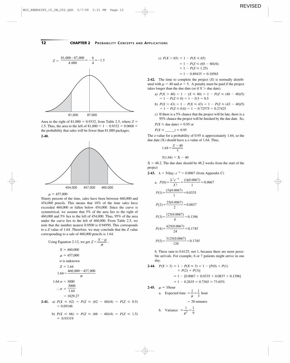
Area to the right of 81,000 � 0.9332, from Table 2.5, where Z �1.5. Thus, the area to the left of 81,000 � 1 � 0.9332 � 0.0668 �the probability that sales will be fewer than 81,000 packages.

2-40.

c) P(X � 65) � 1 � P(X � 65)

� 1 � P(Z � (65 � 60)/4) � 1 � P(Z � 1.25)

� 1 � 0.89435 � 0.10565

2-42. The time to complete the project (X) is normally distrib-uted with � � 40 and � � 5. A penalty must be paid if the projecttakes longer than the due date (or if X � due date).

a) P(X � 40) � 1 � (X � 40) � 1 � P(Z � (40 � 40)/5) � 1 � P(Z � 0) � 1 � 0.5 � 0.5

b) P(X � 43) � 1 � P(X � 43) � 1 � P(Z � (43 � 40)/5) � 1 � P(Z � 0.6) � 1 � 0.72575 � 0.27425

c) If there is a 5% chance that the project will be late, there is a95% chance the project will be finished by the due date. So,

P(X � due date) � 0.95 or

P(X � _____) � 0.95

The z-value for a probability of 0.95 is approximately 1.64, so thedue date (X) should have a z-value of 1.64. Thus,

5(1.64) � X � 40

X � 48.2. The due date should be 48.2 weeks from the start of theproject

2-43. � � 5/day; e�� 0.0067 (from Appendix C)

a.

b. These sum to 0.6125, not 1, because there are more possi-ble arrivals. For example, 6 or 7 patients might arrive in oneday.

2-44. P(X � 3) � 1 � P(X 3) � 1 � [P(0) � P(1) � P(2) � P(3)]

� 1 � [0.0067 � 0.0335 � 0.0837 � 0.1396]

� 1 � 0.2635 � 0.7365 � 73.65%

2-45. � � 3/hour

a. Expected time

� 20 minutes

b. Variance � �1 1

92μ

� �1 1

3μhour

P( )( . )

.53125 0 0067

1200 1745� �

P( )( . )

.4625 0 0067

240 1745� �

P( )( . )

.3125 0 0067

60 1396� �

P( )( . )

.225 0 0067

20 0837� �

P( )( )( . )

.15 0 0067

10 0335� �

Pe

X

x

( )!

( )( . ).0

1 0 0067

10 0067� � �

�λ λ

1 6440

5. �

�X

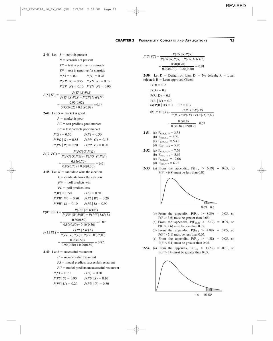
81,000 87,000

454,000 457,000 460,000

� � 457,000Ninety percent of the time, sales have been between 460,000 and454,000 pencils. This means that 10% of the time sales have exceeded 460,000 or fallen below 454,000. Since the curve issymmetrical, we assume that 5% of the area lies to the right of460,000 and 5% lies to the left of 454,000. Thus, 95% of the areaunder the curve lies to the left of 460,000. From Table 2.5, wenote that the number nearest 0.9500 is 0.94950. This correspondsto a Z value of 1.64. Therefore, we may conclude that the Z valuecorresponding to a sale of 460,000 pencils is 1.64.

Using Equation 2-12, we get

X � 460,000

� � 457,000

� is unknown

Z � 1.64

1.64 � � 3000

� � �

� 1829.27

2-41. a) P(X � 62) � P(Z � (62 � 60)/4) � P(Z � 0.5) � 0.69146

b) P(X � 66) � P(Z � (66 � 60)/4) � P(Z � 1.5) � 0.93319

3000

1 64.

1 64460 000 457 000

., ,

��

σ

ZX

��μσ

:



2-46. Let S � steroids present

N � steroids not present

TP � test is positive for steroids

TN � test is negative for steroids

P(S ) � 0.02 P(N ) � 0.98

P(TP | S ) � 0.95 P(TN | S ) � 0.05

P(TP | N ) � 0.10 P(TN | N ) � 0.90

P S TPP TP S P S

P TP S P S P TP N P N( | )

( | ) ( )

( | ) ( ) ( | ) ( )�

�

�00 95 0 02

0 95 0 02 0 10 0 980 16

. ( . )

. ( . ) . ( . ).

�=

P G PGP PG G P G

P PG G P G P PG P P P( | )

( | ) ( )

( | ) ( ) ( | ) ( )�

�

�00 85 0 70

0 85 0 70 0 20 0 300 91

. ( . )

. ( . ) . ( . ).

��

2-47. Let G � market is good

P � market is poor

PG � test predicts good market

PP � test predicts poor market

P(G ) � 0.70 P(P) � 0.30

P(PG | G ) � 0.85 P(PP | G ) � 0.15

P(PG | P ) � 0.20 P(PP | P ) � 0.90

2-48. Let W � candidate wins the election

L � candidate loses the election

PW � poll predicts win

PL � poll predicts loss

P(W) � 0.50 P(L) � 0.50

P(PW | W ) � 0.80 P(PL | W ) � 0.20

P(PW | L) � 0.10 P(PL | L) � 0.90

P W PWP PW W P W

P PW W P W P PW L P L( | )

( | ) ( )

( | ) ( ) ( | ) ( )�

�

�00 80 0 50

0 80 0 50 0 10 0 500 89

. ( . )

. ( . ) . ( . ).

��

P L PLP PL L P L

P PL L P L P PL W P W( | )

( | ) ( )

( | ) ( ) ( | ) ( )�

�

�00 90 0 50

0 90 0 50 0 20 0 500 82

. ( . )

. ( . ) . ( . ).

��

2-49. Let S � successful restaurant

U � unsuccessful restaurant

PS � model predicts successful restaurant

PU � model predicts unsuccessful restaurant

P(S ) � 0.70 P(U ) � 0.30

P(PS | S ) � 0.90 P(PU | S ) � 0.10

P(PS | U ) � 0.20 P(PU | U ) � 0.80

P S PSP PS S P S

P PS S P S P PS U P U( | )

( | ) ( )

( | ) ( ) ( | ) ( )�

�

�00 90 0 70

0 90 0 70 0 20 0 300 91

. ( . )

. ( . ) . ( . ).

��

2-50. Let D � Default on loan; D' � No default; R � Loanrejected; R � Loan approved Given:

P(D) � 0.2

P(D') � 0.8

P(R | D) � 0.9

P(R' | D') � 0.7(a) P(R | D') � 1 � 0.7 � 0.3

(b)

2-51. (a) F0.05, 5, 10 � 3.33(b) F0.05, 8.7 � 3.73(c) F0.05, 3, 5 � 5.41(d) F0.05, 10. 4 � 5.96

2-52. (a) F0.01, 15, 6 � 7.56(b) F0.01, 12, 8 � 5.67(c) F0.01, 3, 5 � 12.06(d) F0.01, 9, 7 � 6.72

2-53. (a) From the appendix, P(F3,4 � 6.59) � 0.05, so P(F � 6.8) must be less than 0.05.

P D RP R D P D

P R D P D P R D P D( ' | )

( | ') ( ')

( | ') ( ') ( | ) ( )

. ( . )

. ( .

=+

= 0 3 0 8

0 3 0 88 0 9 0 20 57

) . ( . ).

+=

6.59 6.80.05

15.52140.01

(b) From the appendix, P(F7,3 � 8.89) � 0.05, so P(F � 3.6) must be greater than 0.05.

(c) From the appendix, P(F20,20 � 2.12) � 0.05, so P(F � 2.6) must be less than 0.05.

(d) From the appendix, P(F7,5 � 4.88) � 0.05, so P(F � 5.1) must be less than 0.05.

(e) From the appendix, P(F7,5 � 4.88) � 0.05, so P(F � 5.1) must be greater than 0.05.

2-54. (a) From the appendix, P(F5,4 � 15.52) � 0.01, so P(F � 14) must be greater than 0.05.



This area is 1 � 0.7257, or 0.2743. Therefore, the probability ofselling more than 265 boats � 0.2743.

For a sale of fewer than 250 boats:

X � 250

� � 250

� � 25However, a sale of 250 boats corresponds to � � 250. At thispoint, Z � 0. The area under the curve that concerns us is that halfof the area lying to the left of � � 250. This area � 0.5000. Thus,the probability of selling fewer than 250 boats � 0.5.

2-57. � � 0.55 inch (average shaft size)

X � 0.65 inch

� � 0.10 inch

Converting to a Z value yields

Z �

�

�

� 1

We thus need to look up the area under the curve that lies to theleft of 1�. From Table 2.5, this is seen to be � 0.8413. As seenearlier, the area to the left of � is � 0.5000.

We are concerned with the area between � and � � 1�. Thisis given by the difference between 0.8413 and 0.5000, and it is0.3413. Thus, the probability of a shaft size between 0.55 inch and0.65 inch � 0.3413.

0 10

0 10

.

.

0 65 0 55

0 10

. .

.

�

X �μσ

� = 0.55 X = 0.65

0.55 0.65

2-58. Greater than 0.65 inch:area to the left of 1� � 0.8413

area to the right of 1� � 1 � 0.8413� 0.1587

Thus, the probability of a shaft size being greater than 0.65 inch is0.1587.

(b) From the appendix, P(F6,3 � 27.91) � 0.01, so P(F � 30) must be less than 0.01.

(c) From the appendix, P(F10,12 � 4.30) � 0.01, so P(F � 4.2) must be greater than 0.01.

(d) From the appendix, P(F2,3 � 30.82) � 0.01, so P(F � 35) must be less than 0.01.

(e) From the appendix, P(F2,3 � 30.82) � 0.01, so P(F � 35) must be greater than 0.01.

� = 250 X = 265

2-55. X � 280

� � 250

� � 25

� Z �

�

�

� 1.20 standard deviations

30

25

280 250

25

�

X �μσ

� = 250 280

From Table 2.5, the area under the curve corresponding to a Z of1.20 � 0.8849. Therefore, the probability that the sales will be lessthan 280 boats is 0.8849.

2-56. The probability of sales being over 265 boats:

X � 265

� � 250

� � 25

� 0.60

�15

25

Z ��265 250

25

From Table 2.5, we find that the area under the curve to the left ofZ � 0.60 is 0.7257. Since we want to find the probability of sellingmore than 265 boats, we need the area to the right of Z � 0.60.



The shaft size between 0.53 and 0.59 inch:

X2 � 0.53 inchX1 � 0.59 inch� � 0.55 inch

Converting to scores:

Z1 � Z2 �

� �

� �

� 0.4 � �0.2

Since Table 2.5 handles only positive Z values, we need to calcu-late the probability of the shaft size being greater than 0.55 �0.02 � 0.57 inch. This is determined by finding the area to the leftof 0.57, that is, to the left of 0.2�. From Table 2.5, this is 0.5793.The area to the right of 0.2� is 1 � 0.5793 � 0.4207. The area to the left of 0.53 is also 0.4207 (the curve is symmetrical). Thearea to the left of 0.4� is 0.6554. The area between X1 and X2 is0.6554 � 0.4207 � 0.2347. The probability that the shaft will bebetween 0.53 inch and 0.59 inch is 0.2347.Under 0.45 inch:

X � 0.45

� � 0.55

� � 0.10

Z �

�

�

� �1

�0 10

0 10

.

.

0 45 0 55

0 10

. .

.

�

X �μσ

�0 02

0 10

.

.

0 04

0 10

.

.

0 53 0 55

0 10

. .

.

�0 59 0 55

0 10

. .

.

�

X 2 �μσ

X1 �μσ

0.53 � = 0.55 0.59

0.45 0.55

Thus, we need to find the area to the left of 1�. Again, since Table2.5 handles only positive values of Z, we need to determine thearea to the right of 1�. This is obtained by 1 � 0.8413 � 0.1587(0.8413 is the area to the left of 1�). Therefore, the area to the leftof �1� � 0.1587 (the curve is symmetrical). Thus, the probabilitythat the shaft size will be under 0.45 inch is 0.1587.

2-59.

x � 3n � 4q � 15/20 � .75p � 5/20 � .25

(4)(.0156)(.75) �

[probability that Marie will win 3 games]

[probability that Marie willwin all four games againstJan]

Probability that Marie will be number one is .04694 � .003906 �.05086.

2-60. Probability one will be fined �

P(2) � P(3) � P(4) � P(5)

� 1 � P(0) � P(1)

� 1 � .03125 � .15625

�

P(0) � 0.03125

P(5) � 0.03125

.08125

= 1 5 5 5 505 0 5

15 1 4− ( ) − ( )(. ) (. ) (. ) (. )

44 25 75 0039064 0( )(. ) (. ) .�

.0464

4

3 4 325 753!

!( )!(. ) (. )

−�

34 25 753⎛

⎝⎞⎠ (. ) (. )�

xn qx n x⎛

⎝⎞⎠

−p

X P(X )

0 .327

1 .410

2 .205

3 .051

4 .0064

5 .00032

1.055 (.2) (.8) .000325 5 5⎛

⎝⎞⎠ =−

45 (.2) (.8) .00644 5 4⎛

⎝⎞⎠ =−

35 (.2) (.8) .0513 5 3⎛

⎝⎞⎠ =−

25 (.2) (.8) .2052 5 2⎛

⎝⎞⎠ =−

15 (.2) (.8) .4101 5 1⎛

⎝⎞⎠ =−

05 (.2) (.8) .3270 5⎛

⎝⎞⎠ =

2-61.



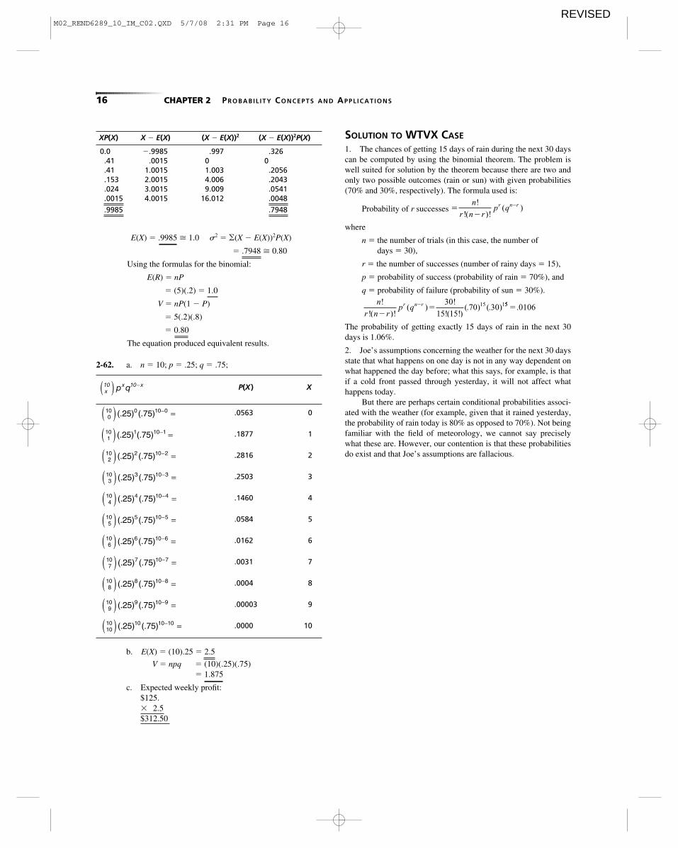
SOLUTION TO WTVX CASE

1. The chances of getting 15 days of rain during the next 30 dayscan be computed by using the binomial theorem. The problem iswell suited for solution by the theorem because there are two andonly two possible outcomes (rain or sun) with given probabilities(70% and 30%, respectively). The formula used is:

Probability of r successes

where

n � the number of trials (in this case, the number of days � 30),

r � the number of successes (number of rainy days � 15),

p � probability of success (probability of rain � 70%), and

q � probability of failure (probability of sun � 30%).

The probability of getting exactly 15 days of rain in the next 30days is 1.06%.

2. Joe’s assumptions concerning the weather for the next 30 daysstate that what happens on one day is not in any way dependent onwhat happened the day before; what this says, for example, is thatif a cold front passed through yesterday, it will not affect whathappens today.

But there are perhaps certain conditional probabilities associ-ated with the weather (for example, given that it rained yesterday,the probability of rain today is 80% as opposed to 70%). Not beingfamiliar with the field of meteorology, we cannot say preciselywhat these are. However, our contention is that these probabilitiesdo exist and that Joe’s assumptions are fallacious.

n

r n rp qr n r!

!( )!( )

!

!( !)(. ) (. )

�� 30

15 1570 3015 155 0106�.

��

�n

r n rp qr n r!

!( )!( )

P(X ) X

.0563 0

.1877 1

.2816 2

.2503 3

.1460 4

.0584 5

.0162 6

.0031 7

.0004 8

.00003 9

.0000 101010 10 10 10(.25) (.75)( ) =−

910 9 10 9(.25) (.75)( ) =−

810 8 10 8(.25) (.75)( ) =−

710 7 10 7(.25) (.75)( ) =−

610 6 10 6(.25) (.75)( ) =−

510 5 10 5(.25) (.75)( ) =−

410 4 10 4(.25) (.75)( ) =−

310 3 10 3(.25) (.75)( ) =−

210 2 10 2(.25) (.75)( ) =−

110 1 10 1(.25) (.75)( ) =−

010 0 10 0(.25) (.75)( ) =−

x10 x 10 xp q( ) −

b. E(X) � (10).25 � 2.5

V � npq � (10)(.25)(.75)� 1.875

c. Expected weekly profit:$125.�1 2.5$312.50

2-62. a. n � 10; p � .25; q � .75;

XP(X) X � E(X) (X � E(X))2 (X � E(X))2P(X)

0.0 �.9985 .997 .326.41 .0015 0 0.41 1.0015 1.003 .2056.153 2.0015 4.006 .2043.024 3.0015 9.009 .0541.0015 4.0015 16.012 .0048

.9985 .7948

E(X) � .9985 � 1.0 �2 � �(X � E(X))2P(X)

� .7948 � 0.80

Using the formulas for the binomial:

E(R) � nP

� (5)(.2) � 1.0

V � nP(1 � P)

� 5(.2)(.8)

� 0.80

The equation produced equivalent results.


Documents

Probability Concepts and Applications - Bilal Bajwa